Universality of parametric Coupling Flows over parametric diffeomorphism

$C^{k}$-diffeomorphisms. Consider an invertible map $f$ from $\mathbb{R}^{d}$ to $\mathbb{R}^{d}$. $f$ is said to be a $C^{k}$-diffeomorphism, if $f$ has up to $k$-th continuous derivatives, and $\det|Df(\bm{x})|\neq 0$ for all $\bm{x}$ . Here $Df$ is the Jaccobian matrix of $f$.

$C^{k}$-diffeomorphism group. One can easily verify that, given $f,g:C^{k}$ diffeomorphisms from $\mathbb{R}^{d}$ to $\mathbb{R}^{d}$, $f\circ g:f\circ g(\bm{x})=f(g(\bm{x}))$ and $f^{-1}$ is still a $C^{k}$-diffeomorphism from $\mathbb{R}^{d}$ to $\mathbb{R}^{d}$. From all above, if we denote

we see that $\text{Diff}^{k}(\mathbb{R}^{d})$ has a natural group structure with composition as its group operator.

Compactly supported $C^{k}$-diffeomorphisms. In real applications, finite data cannot cover the whole space $\mathbb{R}^{d}$. Besides, existing approximation theories only guarantee the capability over some bounded compact set $K$. Due to this two facts, it is more appropriate to consider compactly supported functions or diffeomorphisms. A function $f:\mathbb{R}^{d}\to\mathbb{R}$ is said to be compactly supported, if there exists a compact set $K$ such that $f(\bm{x})=0,\text{ for all }\bm{x}\notin K$. Similarly, a diffeomorphism $f$ is said to be compactly supported, if there exists a compact set $K$ such that $f(\bm{x})=\bm{x},\text{ for all }\bm{x}\notin K$, which can result in that all the components of $Df$ are compactly supported. We define

it is easy to see that $\text{Diff}^{k}_{c}(\mathbb{R}^{d})$ is a subgroup of $\text{Diff}^{k}(\mathbb{R}^{d})$.

Next, we introduce the parametric diffeomorphism.

$C^{k}$-parametric diffeomorphisms. A parametric diffeomorphism is a family of diffeomorphisms with some parameter $\alpha$: $\{f_{\alpha}\}_{\alpha\in A}$, where for any given $\alpha$, $f_{\alpha}$ is a $\mathbb{R}^{d}\to\mathbb{R}^{d}$ diffeomorphism. Usually the parameter is described by some vector $\bm{y}\in\mathbb{R}^{m}$, and $f_{\bm{y}}$ varies continuously or smoothly w.r.t. $\bm{y}$. We denote $f(\bm{y},\bm{x})=f_{\bm{y}}(\bm{x})$. For such a parametric diffeomorphism, we can embed it into a higher dimensional diffeomorphism $F(\bm{y},\bm{x})=\big(\bm{y},f(\bm{y},\bm{x})\big)$. One can verify directly that $F\in\text{Diff}^{k}(\mathbb{R}^{m+d})$ given that (1) $f({\bm{y}_{0},\bm{x}})\in\text{Diff}^{k}(\mathbb{R}^{d})$ for any fixed ${\bm{y}_{0}}$; (2) $f$ is $k$-th differentiable w.r.t. $(\bm{y},\bm{x})$. It is obvious that

whose elements keep the first $m$ coordinates and change the last $d$ ones, is a subgroup of $\text{Diff}_{c}^{k}(\mathbb{R}^{m+d})$.

Here we introduce the classical INNs and investigate the (parametric) diffeomorphism space generated by them.

Invertible linear transforms. First, let us define an elementary group of diffeomorphisms - the invertible linear transforms (ILT):

and the parametric case where $\bm{y}$ is included as parameters:

where $\text{GL}_{d}(\mathbb{R})$ denotes the set of all regular matrices on $\mathbb{R}^{d}$. These groups could be powerful when combined with nonlinear transforms.

Coupling flows. We further define invertible coupling flows which are some specific nonlinear transforms:

where $\phi(\bm{x}_{\leq i},\cdot):\mathbb{R}^{d-i}\to\mathbb{R}^{d-i}$ is a diffeomorphism for each fixed $\bm{x}_{\leq i}$. Specifically, when $\phi(\bm{x}_{\leq i},\bm{x}_{>i})=\bm{x}_{>i}\odot\exp\left(\sigma(\bm{x}_{\leq i})\right)+t(\bm{x}_{\leq i})$, it is the so-called affine coupling flow and we denote $\Phi_{d,i,\sigma,t}=\Phi_{d,i,\phi}$ for such $\phi$. $\sigma,t$ are some functions with $d-i$ output units, typically modeled with deep neural networks. $\odot$ represents the point-wise product. $\bm{x}_{\leq i}=(x_{1},\cdots,x_{i}),$ $\bm{x}_{>i}=(x_{i+1},\cdots,x_{d})$ for $\bm{x}=(x_{1},\cdots,x_{d})$. Similarly, for parametric cases, we have:

and specifically, $\phi(\bm{y},\bm{x}_{\leq i},\bm{x}_{>i})=\bm{x}_{>i}\odot\exp\left(\sigma(\bm{y},\bm{x}_{\leq i})\right)+t(\bm{y},\bm{x}_{\leq i})$ for affine-type coupling flows and we denote $\Phi_{d,i,m,\sigma,t}=\Phi_{d,i,m,\phi}$ for such $\phi$.

Single-coordinate affine coupling flows. Specifically, we can define a flow with only the last coordinate changed. We call it a single-coordinate affine coupling flow (SACF): Let $\mathcal{H}_{d}$ be a set of functions from $\mathbb{R}^{d}$ to $\mathbb{R}$. We define

$\mathcal{H}$-SACF${}_{d}\triangleq\{\Phi_{d,d-1,\sigma,t}:\sigma,t\in\mathcal{H}_{d-1}\}$, and

$\mathcal{H}$-SACF${}_{m,d}\triangleq\{\Phi_{d,d-1,m,\sigma,t}:\sigma,t\in\mathcal{H}_{m+d-1}\}$.

Note that any multi-coordinates affine coupling flows can be represented by finite composition of single-coordinate affine coupling flows, and thus it suffices to just consider the universality of single-coordinate affine coupling flows.

Invertible neural networks. Now let us combine linear invertible transform layers and some coupling flow layers to construct our INNs. Let $\mathcal{G}$ be a set consisting of invertible coupling flows. We define the set of INNs based on $\mathcal{G}$ as

and similarly the parametric case:

When $\mathcal{G}$ contains $\mathcal{H}\text{-SACF}_{d}$ (or $\mathcal{H}\text{-SACF}_{m,d}$ in parametric cases), it is equivalent to replace $\text{ILT}_{d}$ (or $\text{ILT}_{m,d}$) by the symmetric group $S_{d}$ containing all the permutation over $d$ coordinates operating on $\bm{x}$. This type of networks are well known as Real-NVPs [10].

One can also define other types of coupling flows. Nevertheless, the theoretical guarantee of any coupling flow can be verified by simply checking their universality to single-coordinate transforms, which is the main result of our paper as stated in Thm. 3.5.

In this section, we give a definition of universality. For the definition of different functional norms, please refer to Appendix A.

Here we also define distributional universality.

If $\mathcal{M}$ has the $C^{k}$-universality, $\mathcal{M}$ has the $L^{\infty}$-universality because $C^{k}(K)$ is dense in $L^{\infty}(K)$ for any compact $K$. Also, if $\mathcal{M}$ has the $L^{\infty}$-universality, $\mathcal{M}$ has the $L^{p}$-universality for any $1\leq p<\infty$. If an $L^{p}$-universality is satisfied for some $1<p<\infty$, then for any $1\leq q<p$, $L^{q}$-universality is ensured. Finally, $L^{1}$-universality implies distributional universality but the distributional universality does not imply $L^{1}$-universality.

According to the model type, we divide the literature into three categories as follows.

Coupling (or triangular) flows. [21, 5] proved that the distributional universality of a flow family $h$ can be deduced, if $h$ is dense in the set of all monotone functions by pointwise convergence topology. In particular, [19] proved the distributional universality for neural autoregressive flows, and [23] proved the distributional universality for sum-of-square flows. [38] generalized these results, proving that affine coupling flows have $L^{p}$ universality for $1\leq p<\infty$, and autoregsive flows and sum-of-square flows have $L^{\infty}$ universality. However, the approximability to derivatives remains untouched.

Non-triangular flows. The expressiveness of general non-coupling flows is not well studied, as most existing works restrict the form of nonlinearity to certain types, e.g., planar and radial flows [33], Sylvester flows [39], in order to easily compute the determinant of the Jacobian matirx and the inverse maps. [26] gave a first study over some specific distributions, while the universal distributional results still remains unknown. Another type of non-coupling flows, iResNet [4], was proposed based on residual network (ResNet) [18] to improve nonlinearity as well as the computation efficiency of the approximated log determinant. [42] proved that iResNet, capped by a linear layer or with extra dimensions, has $C^{0}$-universality.

Continuous time flows. The ODE-based method is also a major class of flow models as introduced in [7, 16, 8, 36]. [8] gave counterexamples for the $C^{0}$-universality of neural ODEs, however its distributional universality is not yet addressed. An “augmented” neural ODEs was proposed by [12] and then analyzed by [42]. They showed that embedding the original $d$ dimensional neural ODE into a $d+1$ dimensional space can bypass the original counterexamples, achieving a $C^{0}$-universality.

Here we outline the main steps of our proof, and the complete proof is available in Appendix B.

Recall the space $\text{Diff}_{c}^{k}(\mathbb{R}^{d})$: All the $C^{k},\mathbb{R}^{d}\to\mathbb{R}^{d}$ diffeomorphisms which are compactly supported. There are two advantages of choosing $\text{Diff}_{c}^{k}(\mathbb{R}^{d})$ instead of $\text{Diff}^{k}(\mathbb{R}^{d})$ to prove the universality: firstly the compactly supported property greatly simplifies the structure of this group; secondly for any diffeomorphism $F\in\text{Diff}^{k}(\mathbb{R}^{d})$ and any compact set $K$, there exists a compactly supported diffeomorphism $f\in\text{Diff}_{c}^{k}(\mathbb{R}^{d})$ such that $F|_{K}=f|_{K}$, i.e., $F(\bm{x})=f(\bm{x}),\text{ for all }\bm{x}\in K$. Thus, to prove the universality for $\text{Diff}^{k}(\mathbb{R}^{d})$, we only need to consider $\text{Diff}_{c}^{k}(\mathbb{R}^{d})$.

Directly proving the universality to a general diffeomorphism is difficult. It is beneficial to decompose the original hard problem into a series of simpler ones as follows.

One may wonder how many diffeomorphisms can be constructed using a composition of these simple single-coordinate transforms. The answer is surprising: the minimum subgroup containing $S_{c}^{k,d}$ in $\text{Diff}_{c}^{k}(\mathbb{R}^{d})$ is $\text{Diff}_{c}^{k}(\mathbb{R}^{d})$ itself. That is to say, all the diffeomorphisms in $\text{Diff}_{c}^{k}(\mathbb{R}^{d})$ can be constructed from $S_{c}^{k,d}$.

Thm. 3.2 decomposes the original general complex diffeomorphism into finitely-many simple diffeomorphisms. It is natural to ask: if we can approximate all the $S^{k,d}_{c}$ well, can we also approximate $\text{Diff}_{c}^{k}(\mathbb{R}^{d})$ well? Thm. 3.4 gives a positive answer to the question.

Combining Thm. 3.2 and 3.4, noticing that $S_{c}^{k,d}$ is inverse-invariant (for any $\tau\in S_{c}^{k,d},\tau^{-1}\in S_{c}^{k,d}$), we can immediately obtain following theorem.

According to Thm. 3.5, any INNs that approximate $S_{c}^{k,d}$ will eventually approximate $\text{Diff}_{c}^{k}(\mathbb{R}^{d})$. This is a generic result and is first stated in [38] for $L^{p}$ and $L^{\infty}$ cases. We generalize this result to $C^{k}$ cases and also to parametric cases in the next section.

Affine-Coupling Flows. Now we only need to prove the universality of $\mathcal{G}\text{-INN}_{d}$ over $S_{c}^{k,d}$, when $\mathcal{G}$ contains $\mathcal{H}\text{-SACF}_{d}$. However, even for such a simple class of diffeomorphisms, $\mathcal{G}\text{-INN}_{d}$ is not able to approximate it very well: existing works [38] shows that $\mathcal{G}\text{-INN}_{d}$ has $L^{p}$ universality over $S_{c}^{k,d}$. While they gave a negative conjecture for $L^{\infty}$ universality, let alone the $C^{k}$-universality.

However, despite the lack of easily computed log-determinate for density evaluation, when the single-transform is embedded into a higher dimension Euclidean space by padding zeros, the approximation ability becomes much stronger. We prove that the approximation can achieve $C^{k}$-universality, far beyond $L^{p}$ universality. We first define the canonical immersion operator $\iota_{d}$, and its pseudoinverse, canonical submersion $\pi_{d}$:

In Thm. 3.6, we show that by raising the dimension by 1, we can achieve $C^{k}$ -universality. A proof is stated in B.1.3.

We show in Appendix C that, even with this zero-padding, there still exist efficient ways to compute the inverse map of the neural network with a dimension eliminating operator.

Following Section 3.1, we generalize the results to parametric cases, with some changes to cope with parameters.

Recall the definition of compactly supported parametric diffeomorphisms group Eq. (1), where $\bm{y}$ acts as parameters. One might raise a question: why not directly use the result in non-parametric case, as all the elements in $\text{Diff}_{c}^{k,m,d}$ are also in $\text{Diff}_{c}^{k}(\mathbb{R}^{m+d})$? Note that the decomposition theorem only ensures that $S_{c}^{k,m+d}$ can generate $\text{Diff}_{c}^{k}(\mathbb{R}^{m+d})$ and then $\text{Diff}_{c}^{k,m,d}$, it does not guarantee that $S_{c}^{k,m+d}\cap\text{Diff}_{c}^{k,m,d}$, which is the set of transforms acting on a single coordinate of $\bm{x}$, can generate $\text{Diff}_{c}^{k,m,d}$. Without such a guarantee, we have to use operators that may alter coordinates of both $\bm{y}$ and $\bm{x}$, and the coordinates of $\bm{y}$ in the output layer should be exactly the same as the coordinates of $\bm{y}$ in the input layer, which restricts the flexibility and increases the approximation difficulty. Thus we derive new dedicated theorems for parametric cases.

We denote $S_{c}^{k,m,d}\triangleq S_{c}^{k,m+d}\cap\text{Diff}_{c}^{k,m,d}$.

With the assistance of the above theorem, we can easily obtain the $C^{k}$-universality for $\text{Diff}_{c}^{k,m,d}$ by simply following the procedure in section 3.1.

A proof of $\mathcal{G}\text{-INN}_{m,d}$ universality over $S_{c}^{k,m,d}$, when $\mathcal{G}$ contains $\mathcal{H}\text{-SACF}_{m,d}$, follows Thm. 3.6 in section 3.1, and thus the detail of the proof is skipped here.

We demonstrate the expressiveness of our model to learn a parametric diffeomorphism with a synthetic task called “Taiji”. The result demonstrates that, not only the $0$-th order information, but also the $1$-st order information (derivatives) can be learned with good accuracy.

We define our target parametric diffeomorphism:

On the unit circle $\rho=1$, it is not differentiable, thus we expect the trained model to have irregular derivatives over the unit circle, while maintain accurate derivatives elsewhere.

First, we design a task with sufficient amount of data to verify the $C^{1}$ approximation ability of Para-CFlows. We generate samples $\{(\bm{x}_{i},y_{i})\}_{1\leq i\leq 30000}$ with $\bm{x}_{i}\sim\mathcal{U}[-1,1]^{2}$ and $y_{i}\sim\mathcal{U}[0,1]$ independently. Under the polar coordinate representation, i.e., $\bm{x}_{i}=(\rho_{i}\cos\theta_{i},\rho_{i}\sin\theta_{i})$, we calculate the target $f_{y_{i}}(\bm{x}_{i})=(\rho_{i}\cos\tilde{\theta}_{i},\rho_{i}\sin\tilde{\theta}_{i})$ according to Eq. (4). We use a 6-layers affine coupling flows, each layer composed with a random permute. The coupling functions $\sigma,t$ are implemented by 1-hidden-layer Multi-Layer Perceptron (MLP) with hidden-unit number comparable to input dimension. We pad a zero to the input $\bm{x}$, and use the first two output dimensions to compute the loss.

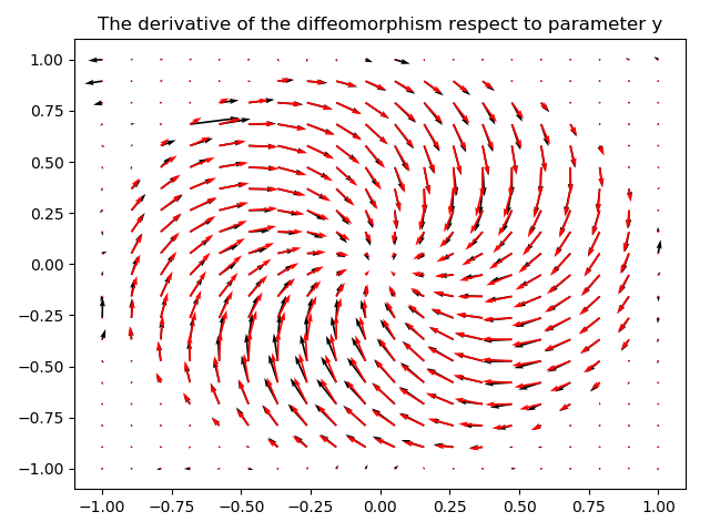
On the left panel of Fig. 2, we observe good consistency between the trained model $\hat{f}_{y}(\bm{x})$ and $f_{y}(\bm{x})$, when $y\in[0,1]$. Note that we only use samples with $y_{i}\in[0,1]$ for training, and thus the model generalizability to $y>1$ is not guaranteed. However, as the true diffeomorphism satisfies $f_{y_{1}}\circ f_{y_{2}}=f_{y_{1}+y_{2}}$, we iterate the trained model recurrently and expect the final output to achieve the effect for $y>1$. The results on the right panel of Fig. 2 justify that the cumulative error from composition does not grow fast, and our model can approximate complex diffeomorphisms with sufficient layers. In Fig. 3 we plot the derivatives of Para-CFlow, compared to the true one. The non-differentiability of the groundtruth on the unit circle results in irregular behaviors of trained model near the unit circle; elsewhere it shows good consistency.

Next we design a more challenging task to compare Para-CFlow against a simple MLP with a hidden-layer-setting as $(128,64,32)$, and Residual Nets (Resnet) [18], that concatenates $\bm{y}$ and $\bm{x}$ as the network’s input and then appends $\bm{x}$ to the output of each layer forward for prediction. Unlike the previous experiment where a scalar $y$ is used, we generate 3000 samples of a 100-dimensional parameter vector $\bm{y}_{i}=(y_{i}^{(1)},\cdots,y_{i}^{(100)})$ where $y_{i}^{(j)}\sim\mathcal{N}(y_{i},0.16)$ and $y_{i}\sim\mathcal{U}[0,1]$. Then $(\bm{x}_{i},\bm{y}_{i})$ is fed to each model to learn the target $f_{\text{avg}(\bm{y}_{i})}(\bm{x}_{i})$. Fig. 4 shows that Para-CFlow learn a much more continuous mapping than MLP and Resnet. While Resnet learns relatively better the outer part than MLP, similar to MLP it suffers from bad mapping in the inner part, i.e. the grey area inside the unit circle is much larger than Para-Flow, which represents bad continuity of the learnt mapping.

The performance of contextual BO depends not only on the exploration-exploitation strategy but also the surrogate model. Ensemble of neural networks is widely used for surrogate and uncertainty modeling, which is flexible for single or multiple outputs [28].

In this section, we ensemble Para-CFlows as a novel surrogate model for BO. We set our experiments with three well-known benchmark functions: Ackley, Trid and Rastrigin [37], which have different features. Note that the original benchmark tasks are contextless, here we simply set the first $d_{c}$ dimensions as the context vector sampled from a multivariate uniform distribution and leave the last dimension as the action to optimize. To construct context-dominating tasks where the reward depends much more on the context than the action, we set $d_{c}\gg 1$. More details are available in Appendix D.

In all benchmarks above, the contexts $\bm{c}$ are uniformly sampled at random from $[-3,3]^{d_{c}}$ sequentially while the action $a$ is optimized over $\texttt{linspace}(-3,3,100)$. To compare different surrogate models, we report the cumulative regrets w.r.t. the optimum alongside the context sequence.

The used ensemble-like surrogate models for contextual BO are listed as follows: (1) Para-CFlow: Ensemble of Para-CFlows for prediction with uncertainty; (2) MLP: Ensemble of MLPs for uncertainty modelling by concatenating context $\bm{c}$ and $a$ to obtain input $(\bm{c},a)\in\mathbb{R}^{d_{c}+1}$; (3) MLP-Ascend: Similar to MLP, the difference is that it firstly raises both $\bm{c}$ and $a$ to the same hidden dimension $\max(5,d_{c})$ and then concatenates them as inputs to a MLP; (4) Resnet: Ensemble of multiple Resnet that concatenates $\bm{c}$ and $a$ as the network’s input and then appends $a$ to the output of each layer forward for prediction.

We implement each of the aforementioned neural networks with similar sizes (details can refer to Appendix D.1) using PyTorch [31]. We ensemble 5 base models as the surrogate model and use the empirical standard deviation of the base model outputs as the uncertainty measurement. We use Lower Confidence Bound (LCB) with $\kappa=1$ as trade-off strategy (The results of using Thompson’s sampling [35] are presented in Appendix D.2) and repeat BO with different surrogates for 10 trails for each experiment setting. In the first 100 steps, we draw a same batch of uniform random samples of $a$ to initialize all surrogates. After that we conduct BO step-by-step and update the surrogates per 100 steps using newly collected samples respectively.

We report the mean and standard deviation of the cumulative regrets for different surrogate models in Fig. 5. The dimensionality of context is set to 5, 10, 20, which is significantly greater than that of action, to demonstrate the capability of Para-CFlow in preserving the sensitivity of action. We observe a significant improvement in optimization for applying Para-CFlow in neural surrogate modeling, which is probably because it preserves all the information of action, whereas compared methods do not. To further verify this conjecture, we train all models with uniformly randomly sampled data (both context and action) of various sizes on Trid and then test the trained models on 10,000 testing contexts, each with sweeping the action space. We calculate the Kendall’s Tau (KT) score [24] between $f_{c}(a)$ and $\hat{f}_{c}(a)$, which measures the action order consistency between the groundtruth and the prediction. As shown in Fig. 6, Para-CFlow exhibits higher KT scores than the other models under higher dimensional context, which demonstrate that it indeed preserves critical information of the action.

References

- [1] Robin Allesiardo, Raphaël Féraud, and Djallel Bouneffouf. A neural networks committee for the contextual bandit problem. In ICONIP, 2014.
- [2] Lynton Ardizzone, Jakob Kruse, Sebastian J. Wirkert, Daniel Rahner, Eric Pellegrini, Ralf S. Klessen, Lena Maier-Hein, Carsten Rother, and U. Köthe. Analyzing inverse problems with invertible neural networks. ArXiv, abs/1808.04730, 2019.
- [3] A. Banyaga. The Structure of Classical Diffeomorphism Groups. Springer US, 1997.
- [4] Jens Behrmann, David Kristjanson Duvenaud, and Jörn-Henrik Jacobsen. Invertible residual networks. In ICML, 2019.
- [5] Vladimir Bogachev, Alexander V. Kolesnikov, and Kirill Medvedev. Triangular transformations of measures. Sbornik Mathematics, 196:309–335, 2004.
- [6] W. M. Boothby. An introduction to differentiable manifolds and riemannian geometry. 1975.
- [7] Changyou Chen, Chunyuan Li, Liquan Chen, Wenlin Wang, Yunchen Pu, and Lawrence Carin. Continuous-time flows for efficient inference and density estimation. In ICML, 2018.
- [8] Tian Qi Chen, Yulia Rubanova, Jesse Bettencourt, and David Kristjanson Duvenaud. Neural ordinary differential equations. In NeurIPS, 2018.
- [9] Youngseog Chung, Ian Char, Willie Neiswanger, Kirthevasan Kandasamy, Andrew, Oakleigh Nelson, Mark D. Boyer, Egemen Kolemen, and Jeff G. Schneider. Offline contextual bayesian optimization for nuclear fusion. ArXiv, abs/2001.01793, 2020.
- [10] Laurent Dinh, Jascha Sohl-Dickstein, and Samy Bengio. Density estimation using real nvp. abs/1605.08803, 2016.
- [11] Laurent Dinh, Jascha Sohl-Dickstein, and Samy Bengio. Density estimation using real nvp. ArXiv, abs/1605.08803, 2017.
- [12] Emilien Dupont, A. Doucet, and Yee Whye Teh. Augmented neural odes. In NeurIPS, 2019.
- [13] David G. Ebin and Jerrold E. Marsden. Groups of diffeomorphisms and the motion of an incompressible fluid. Annals of Mathematics, 92:102, 1970.
- [14] Raphaël Féraud, Robin Allesiardo, Tanguy Urvoy, and Fabrice Clérot. Random forest for the contextual bandit problem. In AISTATS, 2016.
- [15] Alfred Galichon. Optimal transport methods in economics. 2016.
- [16] Will Grathwohl, Ricky T. Q. Chen, Jesse Bettencourt, Ilya Sutskever, and David Kristjanson Duvenaud. Ffjord: Free-form continuous dynamics for scalable reversible generative models. ArXiv, abs/1810.01367, 2019.
- [17] David F. Griffiths, Andrew M. Stuart, and H. C. Yee. Numerical wave propagation in an advection equation with a nonlinear source term. SIAM Journal on Numerical Analysis, 29:1244–1260, 1992.
- [18] Kaiming He, X. Zhang, Shaoqing Ren, and Jian Sun. Deep residual learning for image recognition. 2016 IEEE Conference on Computer Vision and Pattern Recognition (CVPR), pages 770–778, 2016.
- [19] Chin-Wei Huang, David Krueger, Alexandre Lacoste, and Aaron C. Courville. Neural autoregressive flows. ArXiv, abs/1804.00779, 2018.
- [20] Frank Hutter, Holger H. Hoos, and Kevin Leyton-Brown. Sequential model-based optimization for general algorithm configuration. In LION, 2011.
- [21] Aapo Hyvärinen and Petteri Pajunen. Nonlinear independent component analysis: Existence and uniqueness results. Neural networks : the official journal of the International Neural Network Society, 12 3:429–439, 1999.
- [22] Pavel Izmailov, P. Kirichenko, Marc Finzi, and Andrew Gordon Wilson. Semi-supervised learning with normalizing flows. ArXiv, abs/1912.13025, 2020.
- [23] Priyank Jaini, Kira A. Selby, and Yaoliang Yu. Sum-of-squares polynomial flow. ArXiv, abs/1905.02325, 2019.
- [24] M. G. Kendall. A new measure of rank correlation. Biometrika, 30(1/2):81–93, 1938.
- [25] Diederik P. Kingma and Prafulla Dhariwal. Glow: Generative flow with invertible 1x1 convolutions. In NeurIPS, 2018.
- [26] Zhifeng Kong and Kamalika Chaudhuri. The expressive power of a class of normalizing flow models. ArXiv, abs/2006.00392, 2020.
- [27] Andreas Krause and Cheng Soon Ong. Contextual gaussian process bandit optimization. In NIPS, 2011.
- [28] Balaji Lakshminarayanan, Alexander Pritzel, and Charles Blundell. Simple and scalable predictive uncertainty estimation using deep ensembles. In Advances in Neural Information Processing Systems, 2017.
- [29] Christos Louizos and Max Welling. Multiplicative normalizing flows for variational bayesian neural networks. In ICML, 2017.
- [30] Mohammad Mozaffari, Walid Saad, Mehdi Bennis, and Mérouane Debbah. Wireless communication using unmanned aerial vehicles (uavs): Optimal transport theory for hover time optimization. IEEE Transactions on Wireless Communications, 16:8052–8066, 2017.
- [31] Adam Paszke, Sam Gross, Francisco Massa, Adam Lerer, James Bradbury, Gregory Chanan, Trevor Killeen, Zeming Lin, Natalia Gimelshein, Luca Antiga, Alban Desmaison, Andreas Kopf, Edward Yang, Zachary DeVito, Martin Raison, Alykhan Tejani, Sasank Chilamkurthy, Benoit Steiner, Lu Fang, Junjie Bai, and Soumith Chintala. Pytorch: An imperative style, high-performance deep learning library. In Advances in Neural Information Processing Systems 32, pages 8024–8035. 2019.
- [32] Gabriel Peyré and Marco Cuturi. Computational optimal transport: With applications to data science. 2019.
- [33] Danilo Jimenez Rezende and Shakir Mohamed. Variational inference with normalizing flows. In ICML, 2015.
- [34] Elon D. Rimon and Daniel E. Koditschek. The construction of analytic diffeomorphisms for exact robot navigation on star worlds. Proceedings, 1989 International Conference on Robotics and Automation, pages 21–26 vol.1, 1989.
- [35] Daniel J. Russo, Benjamin Van Roy, Abbas Kazerouni, Ian Osband, and Zheng Wen. A tutorial on Thompson sampling. Foundations and Trends in Machine Learning, 11(1):1–96, 2018.
- [36] Hadi Salman, Payman Yadollahpour, Tom Fletcher, and Nematollah Batmanghelich. Deep diffeomorphic normalizing flows. ArXiv, abs/1810.03256, 2018.
- [37] Sonja Surjanovic and Derek Bingham. Optimization test functions and datasets. http://www.sfu.ca/~ssurjano/optimization.html/, 2017.
- [38] Takeshi Teshima, Isao Ishikawa, Koichi Tojo, Kenta Oono, Masahiro Ikeda, and Masashi Sugiyama. Coupling-based invertible neural networks are universal diffeomorphism approximators. ArXiv, abs/2006.11469, 2020.
- [39] Rianne van den Berg, Leonard Hasenclever, Jakub M. Tomczak, and Max Welling. Sylvester normalizing flows for variational inference. ArXiv, abs/1803.05649, 2018.
- [40] Aäron van den Oord, Yazhe Li, Igor Babuschkin, Karen Simonyan, Oriol Vinyals, Koray Kavukcuoglu, George van den Driessche, Edward Lockhart, Luis C. Cobo, Florian Stimberg, Norman Casagrande, Dominik Grewe, Seb Noury, Sander Dieleman, Erich Elsen, Nal Kalchbrenner, Heiga Zen, Alex Graves, Helen King, Tom Walters, Dan Belov, and Demis Hassabis. Parallel wavenet: Fast high-fidelity speech synthesis. In ICML, 2018.
- [41] Cédric Villani. Optimal transport: Old and new. 2008.
- [42] Han Zhang, Xi Gao, Jacob Unterman, and Tom Arodz. Approximation capabilities of neural ordinary differential equations. ArXiv, abs/1907.12998, 2019.
- [43] Dongruo Zhou, Lihong Li, and Quanquan Gu. Neural contextual bandits with ucb-based exploration. In ICML, 2020.
Appendix A Different functional norms and corresponding function spaces
Here we introduce some preliminary definitions on function norms and functions spaces involved in this paper.
For a measurable mapping and a subset , we define:
where can be any norm on , as norms on the finite-dimensional vector space are all equivalent. For simplicity, we choose the maximum norm on , i.e., .
We can also consider the norm containing derivative information when is -th differentiable:
where , and
With these norms, we can define corresponding function spaces:
when is compact, , and an important fact is that is dense in under norm. Thus the universality over in -norm is stronger than the universality over in norm, further stronger than the universality over in norm.
Appendix B Proofs
B.1 Proofs for non-parametric case
B.1.1 Proofs for Theorem 3.2
Definition B.1.
Isotopies. An isotopy between two diffeomorphisms is a -map such that the mapping defined by for all satisfies and for all . It turns out that is a continuous path in the group joining to .
Proposition B.2.
(Proposition 1.2.1 in [3]) The group is connected. Moreover, the group of diffeomorphisms with compact supports which are isotopic to the identity map through isotopies coincide with . Here the identity map I means for all .
Definition B.3.
-near-identity -diffeomorphisms. Let be the -norm ball with radius and centered at identity map , that’s to say, . A diffeomorphism is said to be -near-identity, if .
Lemma B.4.
(Lemma 2.1.8 in [3]) For any diffeomorphism and any , there exists a finite sequence of -near-identity diffeomorphisms such that .
Proof.
Note that there exists an isotopy from to such that and . We rewrite and let , we can see that . Take large enough, we can make and close enough such that is -near-identity. ∎
Theorem B.5.
There exists a , such that for any that is -near-identity, f can be written as with and for . If , so are and . Further more, satisfies -near-identity for .
Let denote the projection onto the coordinate. Suppose is compactly supported and sufficiently -close to the identity. Then for any point , the map given by is a diffeomorphism: surjectivity follows from the fact that has compact support, which means and by the continuity of ; injectivity follows from the fact that if for some , then must has zero derivatives at some point , but the derivative of respect to is near 1, a contradiction.
Now given , define and by
where Obviously given and . Also we observe that, is -near-identity, thus
Then we have
and further
If we denote , we get
which proved that is -near-identity. Here are the kronecker symbols and we notice . ∎
Corollary B.6.
There is a such that for any is -near-identity, f can be written as , with for . If is in for some , then so are .
By taking small enough, we can make small enough, thus the in Thm. B.5 can be further decomposed. A simple observation shows that if already preserves some coordinates, then so does . If we set and , by noticing , we can make small enough, thus the decomposition can always be continued until all the coordinates have been decomposed. ∎
B.1.2 Proof for Theorem 3.4
Take any positive number and compact set . Put and Let satisfying
Since any continuous map is uniformly continuous on a compact set, we take a positive number such that for any with ,
From the assumption, we can take satisfying
Then it is clear that by the definition of . Moreover, we have . In fact, we have
for any .
Then for any , we have
Now let’s consider the cumulative error for derivatives. We have
by noticing that
Higher order derivatives can be estimated following the same procedure with more complex computations and reusing of triangular inequality. We can finally arrive at
with only depends on and and their derivatives, doesn’t depend on because are compactly supported, which means they have finite high order derivatives over .
Thus we take , then , and then finished our proof. ∎
B.1.3 Proof for Theorem 3.6
Note that
This can be decomposed into three small steps:
Next let us approximate using the elements in . By definition, can be written as with to be any function, . By assumption, has -universality for , thus we know has universality for . is just a permutation which is already in our layers. can be written as with , . Here is the inverse of w.r.t. because is a monotonic function w.r.t. . Thus, we claim that has universality for . By Thm. 3.4, we know that can be arbitrarily approximated by .
Thus, for any , there exists a such that
and furthermore,
∎
B.2 Proofs for parametric case
B.2.1 Proofs for Theorem 3.7
Definition B.7.
Isotopies along . An isotopy between two diffeomorphisms is a -map such that the mapping defined by for all , and for all . It turns out that is a continuous path in the group joining to .
Theorem B.8.
The group is connected. Moreover, the group of diffeomorphisms with compact supports which are isotopic to the identity map through compactly supported isotopies coincide with . Here the identity map means for all .
For arbitrary , we have a compactly supported -isotopy
given by the proportionately contraction
It is obvious that always lie in , the first -coordinate corresponding to are fixed. By choosing small enough, we can achieve , the -connected neighborhood of .
Thus, there is a prolongation of that is a compactly supported -isotopy from to with . Since compactly supported -isotopy space with first -coordinate fixed is dense in compactly supported -isotopy space with first -coordinate fixed, and since is already on , we can always find a compactly supported -isotopy from to , and thus is isotopic to the identity in . ∎
Follow the same proof in Lem. B.4, we can get the following lemma.
Theorem B.9.
For any diffeomorphism and any of the identity, there exists a finite sequence of -near-identity diffeomorphisms such that .
Appendix C Dimension Eliminating layer for inverse model
Consider a trained affine coupling flow with padding zeros:
here is a trained surrogate of the parametric diffeomorphism . is something we don’t need to consider in the forward map, but must consider when doing inverse map.
Given any point in output domain, we are not able to directly find the cooresponding input point satisfying , because is unknown.
To handle this problem, we can make to be known. The simplest way is to transform it to zeros. We can train such an eliminating maps:
here for all in a certain compact set. Note that the eliminating map is always trainable in the scope of affine coupling structures: let , is approx. invertible, thus for some , a function of and . By the structure of the affine coupling layers,
can always be approximated.
After the eliminating, we finally get a map:
with is neglectable. Thus given any , we can easily compute the original point because such a map is characterized by INN, and thus easy to compute the inverse.