An Asymptotically Optimal Two-Part Fixed-Rate Coding Scheme for Networked Control with Unbounded Noise Thanks: The authors are with the Department of Mathematics and Statistics, Queen’s University, Kingston, Ontario, Canada, K7L 3N6. Email: jonathan.keeler@queensu.ca, tamas.linder@queensu.ca, yuksel@queensu.ca. This work was presented in part at the 2022 IEEE International Symposium on Information Theory, ISIT 2022 [1].
Abstract
It is known that under fixed-rate information constraints, adaptive quantizers can be used to stabilize an open-loop-unstable linear system on driven by unbounded noise. These adaptive schemes can be designed so that they have near-optimal rate, and the resulting system will be stable in the sense of having an invariant probability measure, or ergodicity, as well as boundedness of the state second moment. Although structural results and information theoretic bounds of encoders have been studied, the performance of such adaptive fixed-rate quantizers beyond stabilization has not been addressed. In this paper, we propose a two-part adaptive (fixed-rate) coding scheme that achieves state second moment convergence to the classical optimum (i.e., for the fully observed setting) under mild moment conditions on the noise process. The first part, as in prior work, leads to ergodicity (via positive Harris recurrence) and the second part ensures that the state second moment converges to the classical optimum at high rates. These results are established using an intricate analysis which uses random-time state-dependent Lyapunov stochastic drift criteria as a core tool.
Index Terms:
Networked control, stochastic stability, ergodicity, source coding, quantization, stochastic optimal controlI Introduction
Networked control or information-constrained control refers to control systems in which the controllers, sensors, and systems (actuators/plants) are connected through communication channels or a data-rate constrained network. Thus, there may be a data link between the sensors (which collect information), the controllers (which make decisions), and the actuators (which execute the controller commands). Moreover, the sensors, controllers and the plant themselves could be geographically separated. For such information-constrained control (or networked control) systems, one needs to jointly design encoders and controllers for satisfactory performance, which may have stability or optimality as a design objective.
In cases where stability is the primary design objective, one is typically concerned with the minimum capacity above which stabilization is possible, and there are many results of this flavour in the existing literature (these are discussed in detail in Section I-B).
This paper is primarily concerned with optimality as the primary design objective. In this context, the notion of optimality is the minimization of some cost function over a specified time horizon (which here is infinite), and for the kinds of systems we consider here, one seeks asymptotic bounds on the cost function as the data rate becomes large.
I-A Problem Statement
Let us first introduce the system to be controlled under no information constraints. The optimal cost in this “classical” case will yield a lower bound over all information-constrained policies. Consider the linear (but not necessarily Gaussian) discrete-time multi-dimensional control system,
| (1) |
where the state process , the control , and the noise process live in , and are real matrices, and we assume to be invertible (this can be relaxed to controllability by a sampling argument for stability [2], though in this case the optimality results we present are not maintained).
The initial state may be distributed according to some probability measure on , as long as admits at least the same finite moments as the noise process . That is, whenever for some , we have (this is trivially satisfied if for some ). In addition, we suppose that the initial state is independent of the noise process .
In the classical, fully observed setting, at each time stage , the controller has access to the history . An admissible control policy is a sequence of Borel measurable mappings where is such that it produces the control at each time stage.
The noise process is assumed to be i.i.d., zero-mean with covariance matrix . Furthermore, we suppose that the noise process admits a pdf with respect to the Lebesgue measure on which is positive everywhere (and thus has unbounded support).
For an positive definite matrix , the optimal control problem is to choose a policy which minimizes the infinite-horizon average quadratic form,
| (2) |
where the expectation above is with respect to the policy and denotes the transpose of the column vector .
The following statement is a special case of a well-known result for a more general setup (where, e.g., may not be invertible) and can be obtained by solving the algebraic Riccati equation (see, e.g., [3, Chap. 4.1]. However, we provide a short and direct proof in the Appendix.
Proposition 1.1.
For the fully observed setup described above, the optimal control policy is , achieving an optimal cost of where is the trace operator.
In contrast to this idealized fully observed setup, in this paper we assume that the controller only has access to through a discrete noiseless channel of capacity bits. We assume that the encoder is causal. In particular, letting be a finite alphabet of cardinality , the encoder is specified by a quantization policy , which, with as the state space, is a sequence of functions of the type . At time , the encoder transmits the -valued message
where and for . The collection of all such zero-delay policies is called the set of admissible quantization policies and is denoted by .
Upon receiving , the receiver generates the control , also without delay. A zero-delay controller policy is a sequence of functions such that , where is the control action space, so that , where .
Thus, the data rate is fixed, and we assume zero coding delay. In this setup, it becomes necessary to describe not just a control policy, but also a coding scheme with which to communicate information about the current state vector.
I-B Literature Review
For systems of this nature, various authors have obtained the minimum channel capacity above which stabilization is possible, under various assumptions on the system and the admissible coders and controllers. Here, “stabilization” can be in several senses, for example positive Harris recurrence, asymptotic mean stationarity or more generally, limiting moment stability of the state.
Such a result is usually referred to as a data-rate theorem and takes the following form, with being the eigenvalues of the system matrix :
| (3) |
That is, the capacity must exceed the sum of the unstable eigenvalue logarithms.
Some of the earliest works in this context are [4] and [5]. More general versions of the data-rate theorem have been proven in [6] and [7]. For noisy systems and mean-square stabilization, or more generally, moment-stabilization, analogous data-rate theorems have been proven in [8] and [9], see also [10, 11].
In [12, 13], a joint fixed-rate coding and control scheme is given which, in the scalar case with unstable eigenvalue and where is Gaussian, stabilizes the system (1) while being nearly rate-optimal, in that the rate used satisfies only . This is achieved using an adaptive uniform quantization scheme, where the quantizer bin sizes ”zoom” in and out exponentially to track the state . Here, the notion of stability is ergodicity and finiteness of all limiting system moments. By increasing a sampling period , the achievable rate gets arbitrarily close to [2, Theorem 2.3]. This scheme can be generalized to one which stabilizes the multi-dimensional system (1) (where the noise is more general than Gaussian) using a similar approach [2]. Furthermore, this leads to a closed loop system which is positive Harris recurrent (and hence, ergodic) and admits finite limiting system second moment [2, Theorem 2.2]. For related recent fixed-rate constructions which also utilize modest delay, we refer the reader to [14] and [15].
Despite being near rate-optimal for achieving stability (i.e., finite asymptotic system moments), the schemes in [12, 13, 2] have not been shown to yield second moment convergence to the classical optimum as the data rate grows large.
In the literature, information theoretic relaxations of the problem noted have been studied, for obtaining both lower and upper bounds. Lower bounding methods typically build on replacing the number of bins with entropy of the quantization symbols, or the latter with mutual information bounds, and the use of Shannon lower bounding techniques. Upper bounding methods include entropy coding and dithering methods; dithering [16] “uniformizes” the noise even for low rates (though which critically requires the presence of common randomness at the encoder and the decoder); see [17], [21] [22], [23], [24]. Using ergodicity and invariance properties, [24] has established time-invariant (though still variable-rate) coding schemes using dithering. Making use of lattice quantization performance bounds developed in [19], without the use of of dithering [20] investigated distributed control with lattice quantization followed by entropy coding (and thus also with variable rate coding) and established near optimality of such schemes for high-rates.
In this paper, we will only use fixed-rate codes, which may be more suitable for a large class of zero-delay systems.
A further common approach in the literature has been to minimize the directed information [25] subject to the distortion rate:
This leads to an information theoretic lower bound to the optimal estimation error subject to an information rate constraint. There has been a surge of research activity on this problem since [26], where explicit solutions, bounds, as well as convex analytic numerical solutions (including via semi-definite programming) have been presented; see, e.g., [27, 28, 18, 29, 30, 31, 23, 32, 33, 34]. For noisy channels, using channel-source coding separation based methods via the rate-distortion function and Shannon capacity duality can be utilized to establish tightness results, especially for the Gaussian case. When an additive Gaussian channel is present, sequential rate-distortion theoretic ideas presented above in (also via generalizing the scalar Gaussian analysis [27]) lead to explicit optimality conditions studied in [30] and [35] (see also [20])
I-C Contributions
We study the class of stochastic linear systems having transition dynamics given in (1) and driven by unbounded noise that are to be controlled across a discrete noiseless channel of finite capacity. For such systems, we present a novel two-stage coding scheme, in which the first stage is time-adaptive and stabilizing (in the sense of positive Harris recurrence and finite limiting system moments), while the second stage is fixed in time. The first coding stage is a variation on the schemes in [12, 13, 2].
Crucially utilizing the ergodicity results of the first coding stage, we show that this two-part coding scheme attains convergence of the limiting system second moment to the classical optimum as the data rate grows large, with explicit rate of convergence. While multi-stage quantization schemes have been studied before in the source coding literature [40], our implementation is novel in that one stage of the code is time-adaptive (though still with fixed-rate) and stabilizing, and the second stage is designed for near-optimal performance at high-rates. An inspiration for this approach also comes from Berger [41] and Sahai [42]. Our analysis complements recent studies in the literature [20] [24] which have utilized variable rate codes (without and with dithers, respectively), but more importantly, it presents a two-part architecture in code design, separately targeting stability and optimality.
To our knowledge, this is the first scheme proven to have this convergence property for systems of this type (in particular, with unbounded noise) in networked control. The algorithm to be presented is relatively simple, and being fixed-rate, highly practical, but its performance analysis requires quite involved technical steps which necessitate a technically involved analysis using, among other tools, random-time state-dependent stochastic Lyapunov drift conditions [12] and a careful analysis of the performance of finite-level uniform quantizers for unbounded sources that satisfy certain moment constraints.
I-D Organization
The paper is organized as follows. Section II contains relevant preliminaries, some background on stochastic stability for general state-space Markov chains, and statements of some useful random-time Lyapunov drift theorems that are central to our analysis.
Section III presents the construction of our two-part scheme in the scalar case for simplicity, and provides a somewhat detailed proof program to guide the reader. Section IV provides the construction of our two-part scheme in the vector case, in full generality. A detailed proof program in the vector case is provided in Section IV-D.
Finally, as many of the proofs are rather mechanical and quite involved, the Appendix contains complete proofs of many key results stated in the main body of the paper.
II Preliminaries
II-A Definitions and Conventions
We denote the nonnegative and strictly positive reals by and , respectively. We let denote the nonnegative integers.
For and we denote . For we denote .
It is well-known that is a norm on for all . The following pair of inequalities is also well-known (e.g., see [43, Exercise 3.5(a)]):
Proposition 2.1.
Suppose . Then for any ,
| (4) |
where is taken to be by convention.
The first inequality follows by a simple renormalization argument, while the second follows from Hölder’s inequality.
For a matrix , we will refer to the -th component either as or as . The latter notation will be used when takes on an expression involving square brackets (e.g., an expectation) so as to avoid ambiguity.
For a matrix we define its -norm as . This norm is consistent with the vector -norm in the following sense. Let and . Then,
| (5) |
We will find it useful to use the Landau notation for comparing function asymptotics. For two functions , where , we say that if for all sufficiently large one has for some constant . This is equivalent to the condition that .
Finally, for a vector-valued random variable we denote its “tail function” as
II-B Stochastic Stability
In this section we provide some brief background on stochastic stability, particularly that which will be relevant to the stabilizing properties of the two-stage scheme we present (namely, positive Harris recurrence).
Suppose is a time-homogeneous Markov chain with state space , where is a complete separable metric space that is locally compact; its Borel sigma algebra is denoted . The transition probability is denoted by , so that for any and , the probability of moving in one step from state to the set is given by . For any , the -step transitions are obtained recursively in the usual way:
The transition law acts on measurable functions and measures on via
and
A probability measure on is called invariant if , that is,
For any initial probability measure on we can construct a stochastic process with transition law and . We let denote the resulting probability measure on the sample space, with the usual convention that (i.e., ) when the initial state is . When is invariant, the resulting process is stationary.
There is at most one stationary solution under the following irreducibility assumption. For a set we denote,
| (6) |
Definition 2.2.
Let denote a -finite measure on .
- (i)
The Markov chain is called -irreducible if for any and satisfying we have
- (ii)
A -irreducible Markov chain is aperiodic if for any and any satisfying , there exists such that for all ,
- (iii)
A -irreducible Markov chain is Harris recurrent if for any and any satisfying . It is positive Harris recurrent if in addition there is an invariant probability measure .
The notion of full and absorbing sets will be useful to us.
Definition 2.3.
For a -irreducible Markov chain , a set is called full if .
Definition 2.4.
A set is called absorbing if for all .
Finally, we define the notion of small sets for a Markov chain.
Definition 2.5.
A set is -small on (for integer , and a probability measure on ) if for all and ,
A set is called small (or sometimes -small) if it is -small for some .
Briefly we provide an intuition for small sets. Suppose is -small. Whenever the state happens to visit the set , it forgets its entire past with probability at least and transitions according to the probability measure over the next time stages. In this way, the small set acts as a “regenerative set” from which the process can forget its history. This line of investigation leads one to Nummelin’s splitting technique [44, 45], which is a key tool in many stability results for irreducible Markov chains.
II-C Random-Time State-Dependent Stochastic Lyapunov Drift Conditions for Stability
In this section, we present a drift condition [13] and use it to show two stability results which will be crucial to our analysis. As in the previous section, we consider a general Markov chain . We consider a sequence of stopping times , measurable with respect to the natural filtration of , such that is strictly increasing and . Finally, we will make use of the filtration which is informally the filtration of “information generated by up to time ” (for full details, see [46]).
The following is a condition on the general Markov chain introduced in [13].
Condition 2.1 (Random-Time Lyapunov Drift).
For a measurable function , measurable functions , a constant and a set , we say that satisfies the random-time Lyapunov drift condition at if for all
and
| (7) |
when .
Remark 2.1.
This drift condition, in combination with different assumptions on the functions and sets involved, can lead to many useful results on stability (e.g., [13, Theorem 2.1]). We present two such results here.
Remark 2.2.
The results presented here are variations of [13, Theorem 2.1], presented in the form most useful for our application. The proofs of these results draw heavily from the proof program in [13] and rely on supermartingale arguments. For brevity we have omitted the proofs here; for details, see [46] and [13].
Lemma 2.6.
Suppose is -irreducible and satisfies Condition 2.1 at all , with the restrictions that is a small set, , and . Then the set
is full and absorbing, and the restriction of to is positive Harris recurrent.
If in addition one can show that for all (i.e., ), then is positive Harris recurrent.
Lemma 2.7.
Suppose that is positive Harris recurrent with invariant measure and satisfies Condition 2.1 at some . Then,
and for any function which is bounded by in that for some constant , we have the following ergodic theorem for ,
| (9) |
for every .
III Scalar Linear Systems
We begin with considering the scalar case for simplicity. Here we consider control of the scalar system,
| (10) |
where and the noise process is assumed to be i.i.d., zero-mean with finite second moment . Furthermore, we suppose the noise process admits a pdf with respect to Lebesgue measure on which is positive everywhere. Here we will also suppose that so that the system is open-loop-unstable. That is, if we set for all , then the system is transient and tends to infinity in magnitude (almost surely and in mean-square).
As in Section I-A, may be distributed with some probability measure on , so long as admits the same finite absolute moments as the noise process . In addition, we suppose that the initial state is independent of the noise process .
Then the optimal control problem we study is to choose a policy which minimizes the infinite-horizon quadratic cost,
| (11) |
By Proposition 1.1, in the fully observed setup the optimal control policy is which achieves an optimal cost of . We suppose now that the controller only has access to through a discrete noiseless channel of capacity bits.
Our goal here is to minimize which we know is bounded below by . As the state will only be partially observed by the controller, we seek to arrive at asymptotic bounds on the “optimality gap” in terms of the channel capacity .
We say that is a joint coding and control scheme for if specifies both a coding scheme for communicating over the channel of capacity as well as a corresponding control scheme at the channel receiver.
The following result demonstrates a limit on achievable rates of convergence.
Lemma 3.1.
Under any joint coding and control scheme we have
| (12) |
The proof follows the core arguments of the proof of [47, Theorem 11.3.2] (with several critical changes, as the assumed limit of distortions utilized in [47, Theorem 11.3.2] is to be replaced with a limit of average distortions, requiring additional steps) and is provided in the Appendix.
Intuitively, the above lemma implies that the fastest rate of convergence (of the optimality gap to zero) one can hope for is . Motivated by this, we normalize potential rate functions by and make the following definition.
Definition 3.2.
A joint coding and control scheme achieves second moment convergence with rate function if,
For brevity we may say simply that achieves the rate function .
Intuitively, one seeks to achieve a rate function which grows slowly in order to maximize the rate of convergence. Lemma 3.1 implies that the best achievable rate function is the constant function, so any achievable rate function satisfies .
We will impose the following mild condition on the noise process.
Condition 3.1.
For some , . That is, the noise process has finite th moment.
In the scalar case, our main result is the following.
Theorem 3.3.
Supposing Condition 3.1 holds with , for any there exists a joint coding and control scheme, denoted Scheme P, which achieves the exponential rate function .
Intuitively, with only the condition that the noise admits finite th moment, we are able to construct schemes that nearly (as ) achieve convergence of the optimality gap like . If is quite large, then the convergence becomes much closer to and, in the extreme case where admits finite moments of all orders (such as in the case of a Gaussian), one can construct schemes achieving convergence of the optimality gap at a speed for any .
The rest of Section III is dedicated to the construction of Scheme P and a high-level proof program of Theorem 3.3. All proofs are relegated to the Appendix.
III-A Two-Part Code with Uniform Quantization
In this section we describe the joint coding and control scheme used in proving Theorem 3.3.
The coding scheme is in two parts where the first part is adaptive in time and the second is fixed. The adaptive part will yield stability, and the fixed part will yield an optimal rate of convergence via simple iterated expectation arguments.
To communicate over a finite capacity channel, will employ uniform quantizers. Let be an even integer and be a scalar “bin size”. We define the scalar modified uniform quantizer by,
| (13) |
This quantizer uniformly quantizes into bins of size and maps all larger to zero. This requires output levels.
We will use this quantizer for two different purposes.
- (i)
The first is to use adaptive bin sizes which vary with time to achieve stability (in the sense of positive Harris recurrence and finite system moments). Let be an even integer, and suppose that is a sequence of strictly positive “bin sizes” varying with time. We will make use of the quantizer .
- (ii)
Secondly, we will use this quantizer to achieve optimal convergence. For a given even number of bins , let be a bin size which is a function of . We will make use of the quantizer . For brevity, we denote and where necessary, specify the dependence of on . Note that this quantizer is fixed in time, in contrast to .
Suppose that the sequence of bin sizes is such that is a function of only and the indicator random variable . Also assume that both the encoder and decoder (controller) know . If is sent over the channel, it is possible to synchronize knowledge of between the quantizer and the controller since if and only if .
The coding scheme is constructed as follows. For as above, we calculate the adaptive quantizer output and the adaptive system error . Then for integer we use a fixed quantizer with bin size as mentioned above to calculate the fixed quantizer output . We then send and across the noiseless channel where the channel capacity is at least,
| (14) |
We estimate the state as . To mirror the fully observed case, the controller applies the control
The scheme is illustrated in Figure 2.
The controlled system dynamics resulting from this scheme are
| (15) |
Finally, we describe the adaptive bin size update dynamics where, as in prior work in this context [12, 13], a simple zooming scheme is employed. We assume that is even and large enough that and choose scalars and such that , and . We also assume that . Choose arbitrarily, then for the bin update is
| (16) |
The following result is proved, e.g,. in [13].
The motivation for this scheme is that the adaptive part leads to stability in the sense of positive Harris recurrence, while the fixed quantizer leads to order-optimal convergence of the ergodic second moment (11) as the fixed quantization rate grows large.
The state space for the process highly depends on the following “countability condition”.
Condition 3.2.
There exist relatively prime integers such that . Equivalently, is rational.
If this condition holds, then starting from an arbitrary there exists such that always belongs to a subset of (see e.g. [13, Theorem 3.1]). If the condition fails, then starting from any fixed the set of reachable bin sizes is a dense but countable subset of .
We restrict our analysis to the case where Condition 3.2 holds. This is not restrictive; it can be shown that for any arbitrary there exists arbitrarily close that satisfy Condition 3.2. We let the state space for be
The state space for the Markov chain is then . What remains is to specify additional constraints which complete our proposed scheme.
We assume that Condition 3.1 holds for some . For any we finish our construction of Scheme P by requiring that and specifying the dependence of on as .
Remark 3.1.
In this scheme, the constant multiplying is arbitrary for convergence purposes.
We also impose the following condition in our construction.
Condition 3.3.
The minimum adaptive bin size is at least .
This may place an implicit dependence of on the number of fixed quantization bins , though if all other parameters remain fixed as increases then one can ensure Condition 3.3 holds by ensuring that it holds for (since as specified above is monotone decreasing in ).
Finally, as we fix and let to take advantage of fixed quantization results at high rates, to be presented shortly.
Since the proof of Theorem 3.3 is rather tedious, we present a somewhat detailed proof program to guide the reader for the scalar setup.
We note that while the proof method for stabilization of our scheme builds on the random-time Lyapunov drift approach introduced in [12, 13], the coupling between the two parts of the coding scheme significantly complicates the analysis. Furthermore, we consider performance bounds as the data rate grows without bound. Altogether, this requires a cautious analysis between moments and high-rate quantization coupled with random-time drift criteria.
III-B High-level Proof Program
In this section we outline the high-level proof program for Theorem 3.3, i.e., the proof that Scheme P achieves the exponential rate function . Results without complete proofs admit more general sister results in the vector case, which is discussed in detail in Section IV-D.
Theorem 3.5.
Under Scheme P with , is positive Harris recurrent for every even (i.e., as grows without bound). Therefore, for every even , Scheme P yields a unique invariant measure for the process .
Sketch of Proof.
We establish -irreducibility and aperiodicity for where is the product of the Lebesgue and discrete measures on . The logarithmic function is shown to satisfy Condition 2.1 with constant and (i.e., in the form required by Lemma 2.6), leading to positive Harris recurrence. For a complete proof, see the proof of Theorem 4.6 (vector case). ∎
Remark 3.2.
The analysis here is highly similar to that of the proof of [13, Theorem 3.1]. The only major change is that the upper bound of [13, Lemma 5.2] for the tail probabilities must be re-derived in some form, as the out-of-view state dynamics change significantly due to the fixed quantization stage. We address this by providing a similar bound in Lemma 6.5 (compare to equation (26) in [13]), which decays suitably fast for summability in the proof program under Condition 3.1.
We denote as the state under invariant measure. This will also induce an invariant measure for the system adaptive error , which we denote by .
We have the following ergodicity result.
Proposition 3.6.
The infinite-horizon second moment and the invariant second moment agree, that is
Sketch of Proof.
Finally, we use a simple iterated expectation argument. Suppose that . Let and , where (recall is the distribution of ). Since we have applied the one-step transition kernel and is the invariant measure, the marginal distributions of and are identical.
For brevity, we denote so that . Supposing that (this will be shown as part of the full proof program), we then have by invariance and iterated expectations that
| (17) |
Let denote the system adaptive error under invariant measure, i.e., . Rearranging (17), we find that the optimality gap is given as
| (18) |
which is (up to a constant) the distortion of the fixed quantizer applied to the random variable .
With this in mind, we state the following result for high-rate distortion of on sequences of suitably well-behaved random variables. The proof builds on balancing the trade-off between distortion due to the high-rate granular region and the overflow region.
Lemma 3.7.
Let be a sequence of random variables that satisfy,
| (19) |
for some (not necessarily integer). Set the bin size for the quantizer as . Then we have,
The proof is mostly mechanical; for a proof, see the proof of Lemma 4.5 (vector case) in the Appendix.
Briefly, we note that if the sequence is for instance uniformly sub-Gaussian (in the sense that for some , then (19) holds for every and so it is possible to achieve distortion asymptotic to for any by taking sufficiently large.
However, this sub-Gaussian condition is much stronger than (19), and if one follows the proof of Lemma 3.7 using this stronger tail condition carefully, setting the bin size slightly differently, it is possible to achieve convergence that is faster than (for instance, ).
Remark 3.3.
One can justify that Lemma 3.7 cannot be improved without strengthening the imposed condition or using more complex (i.e., non-uniform) quantizers. Consider the special case where for all and where admits the “Bucklew-Gallagher” pdf,
| (20) |
for arbitrary . This distribution has finite moments only of order and since is independent of , the problem here is essentially optimal quantization of . Let denote the infimum (MSE) distortion achievable over all uniform quantizers with output levels. In [48], it is shown that for the source above, satisfies asymptotically (see the first equation in [48, p. 963]),
for some constant , so that asymptotically the best distortion achievable by uniform quantizers for the above source is .
Now we compare this to Lemma 3.7. Here, since admits finite moments for any , by employing our uniform quantizer with step size we achieve asymptotic distortion . As we let from below, becomes arbitrarily close to and so the result we have stated here achieves asymptotic distortion which can be arbitrarily close to the best achievable asymptotic distortion one can get using uniform quantization. It is in this sense that Lemma 3.7 cannot be improved without strengthening the conditions imposed on the sequence , or without employing more complex quantization schemes.
In light of (18), we would like to apply Lemma 3.7 to the sequence of random variables . To do this, we need to establish (19). This is ensured by the following result.
Lemma 3.8.
Under Scheme P, the invariant system error has finite th moment uniformly in . That is,
| (21) |
Sketch of Proof.
With Lyapunov functions and proportional to and appropriate set and constant , we show that these functions satisfy the drift condition (8). In particular, we do this for proportional to and proportional to which, with the Lyapunov parameters independent of leads to results of the form (21) by Lemma 2.7 for the invariant state and adaptive bin size. A simple invariance argument finishes the result. Condition 3.1 is crucial to the proof of this result. For a complete proof, see the proof of Lemma 4.9 in the Appendix. ∎
IV The Multi-Dimensional Case
We now present the more general vector case. Recall that we consider control of the multi-dimensional system (1) over a discrete noiseless channel of capacity bits and the aim is to minimize the infinite-horizon average quadratic form (2).
As stated earlier, in the fully observed setup the optimal control policy is which achieves an optimal cost of . In light of this, we seek to arrive at asymptotic bounds on the optimality gap,
in terms of the channel capacity .
We first generalize Definition 3.2 to the vector case.
Definition 4.1.
A joint coding and control scheme achieves second moment convergence with rate function if,
For brevity we may say simply that achieves the rate function .
We refer the reader to [49, Theorem 4.2] for a fundamental lower bound which leads the vector analog to the expression presented in Lemma 3.1.
Remark 4.1.
In the vector case, the factor of in the above definition comes intuitively from the fact that to tile a hypercube in of width it takes bins of width .
As in the scalar case, one seeks to achieve a rate function which grows slowly to maximize the rate of convergence.
We will impose the following condition on the noise process, analogous to Condition 3.1.
Condition 4.1.
For some , , i.e., the noise process has finite th moment.
The following generalization of Theorem 3.3 is our main result.
Theorem 4.2.
Supposing Condition 4.1 holds with , for any there exists a joint coding and control scheme Scheme P which achieves the exponential rate function .
IV-A Vector Quantization
In the multi-dimensional case, we will make use of vector quantization. We will use scalar uniform quantizers to define two types of cubic lattice vector quantizers.
Let be an even integer and be a scalar “bin size”. With the usual floor function, we define the partial uniform quantizer as
Note that . Then, we define the type I vector quantizer as
| (22) |
and the type II vector quantizer component-wise as
Remark 4.2.
If then the above definitions both correspond to the scalar quantizer (13). For this reason, the scheme we present for the vector case is a direct generalization of the scalar scheme.
As in the scalar case, we will use these vector quantizers for two different purposes. The type I quantizer will be used with adaptive bin sizes to achieve stability. Let be an even integer, and suppose that is some sequence of strictly positive bin sizes varying with time. We will make use of the quantizer .
The type II quantizer will be used to achieve convergence to the optimum. For a given even number of bins , let be a bin size which is a function of . We will make use of the quantizer . For brevity we denote and where necessary, specify the dependence of on .
IV-B System in a Jordan Form
Briefly, we discuss a reduction of the system matrix into its separate modes. This will have the useful side effect of making very close to the absolute eigenvalue of each mode.
Let be the (possibly repeated) eigenvalues of the system matrix . Without loss of generality, we assume that is in real Jordan normal form, as any matrix there exists an invertible matrix such that is the real Jordan normal form of [50, Theorem 3.4.1.5]. Let and left-multiply the system (1) by . Defining and , the system dynamics become
which is in the same form as (1) but with the system matrix in real Jordan normal form.
For the purposes of controlling this system, it suffices to consider each of the Jordan blocks of individually. Since the matrix is invertible, the control of each of these blocks will be identical to the control problem for the full system (1). Therefore, by a slight abuse of notation, we will consider the control of a single mode or Jordan block (which may now be part of a larger system) with the single repeated eigenvalue . By the real Jordan normal form [50, Theorem 3.4.1.5], we know then that takes the form
| (23) |
where and respectively. For above, is the identity matrix and is the matrix
We note that for in either of the forms above, we can describe quite easily:
Proposition 4.3.
There are four cases to consider, which are:
- •
If and then .
- •
If and then .
- •
If and then .
- •
If and then .
The equalities follow just by observing the rows of under each assumption. In the complex case, the upper bound follows by Cauchy-Schwarz inequality in . The largest upper bound is , so in view of (5) we may always write that
| (24) |
Briefly, we remark that the above bound can be improved in the case by applying an invertible transform . That is, as before we let and apply the same “change-of-view” transformations , and . By left-multiplying the system (1) by we arrive at an identical control problem now with the system matrix .
From here it suffices to determine how small can be made over all invertible transformations . At least in the case we demonstrate that the infimum is at most using the following construction.
First, suppose is a real Jordan block, i.e. that of (23) for . For any we let with inverse . Then,
Therefore, . By taking this value is arbitrarily close to . If one allows for complex vector and matrix entries, an identical argument can be made in the case .
The minimization of will be relevant to our scheme in terms of the minimum capacity required for stabilization.
Remark 4.3.
It is important to distinguish between the cases and . In the former case, the system is open-loop-stable so stability is easy to achieve. Here, if one employs only the fixed quantization stage of the scheme we present in the next section, then stability of the process is nearly automatic and the asymptotic optimality will follow by simple iterated expectation arguments that are almost identical to what we will present shortly. Therefore, we will ignore the stable case and suppose moving forward that .
IV-C Scheme P in the Vector Case
In this section we describe the joint coding and control scheme of Theorem 4.2. The scheme presented is very similar to that of the scalar case and is in fact a direct generalization of the joint scheme of Theorem 3.3.
Let be an even integer and suppose is a sequence of positive “bin sizes” such that is a function of only and the indicator random variable . Also assume that both the encoder and decoder (controller) know . Then so long as the type I quantization is sent over the channel, it is possible to synchronize knowledge of between the quantizer and the controller since if and only if .
The coding scheme is as follows. For as above, we calculate the adaptive quantizer output and the adaptive system error . Then for integer we use a fixed type II quantizer with bin size as in Section IV-A to calculate the fixed quantizer output . We then send and across the noiseless channel where the channel capacity is at least,
| (25) |
We estimate the state as . To mirror the fully observed case, the controller applies the control
The scheme is essentially exactly as illustrated in Figure 2 from the scalar case, where is generalized to .
The controlled system dynamics resulting from this scheme are
| (26) |
The update dynamics for are nearly identical to the scalar case. We assume that and choose scalars , and . We assume again that . Choose arbitrarily, then for the bin update is
| (27) |
The motivation for this scheme is as in the scalar case. The adaptive type I quantizer will lead to stability in the sense of positive Harris recurrence, and the fixed type II quantizer will lead to order-optimal convergence of the system quadratic form under invariant measure as the fixed quantization rate grows large.
As in the scalar case, we impose Condition 3.2 so that the state space for is countable. The state space for is
and the state space for the Markov chain is . What remains is to specify additional constraints which complete our proposed scheme.
We assume that Condition 4.1 holds for some . For any we finish our construction of Scheme P by requiring that and specifying the dependence of on as (again, the constant here is arbitrary).
We impose the following restriction on the minimum bin size which generalizes Condition 3.3 to the vector case.
Condition 4.2.
The minimum adaptive bin size is at least,
Finally, as in the scalar case, as we keep fixed and let to take advantage of fixed quantization results at high rates, to be presented shortly.
IV-D Proof Program for Stability and Convergence
In this section, we outline the proof program for Theorem 4.2, i.e. that Scheme P achieves the exponential rate function . Many of the proofs of intermediate results are tedious and largely mechanical, so we have relegated these to the Appendix.
We first give an intermediate result on high-rate quantizer distortion and then present a high-level proof program of Theorem 4.2 with similar key arguments as those in Section III-B.
Let be a sequence of random vectors on and consider the quantizer described in Section IV-A. We define for the error vectors
Lemma 4.5.
Suppose that
for some (not necessarily integer). Set the bin size for the type II quantizer as . Then for any positive semidefinite matrix we have
The proof is mostly mechanical and can be found in the Appendix.
We denote the “in-view” set 11 1 In [12], this was referred to as the perfectly zoomed phase set as,
i.e., the set of states such that the adaptive quantizer is non-zero.
We will show in Lemma 6.5 that states beginning in this set return to it very quickly, in that for constants and we have
which decays very fast in integer . Essentially all of the following stability results will follow from repeated application of this inequality and Condition 4.1 on the noise process.
Theorem 4.6.
Under Scheme P with , is positive Harris recurrent for every even . Therefore, for every even , Scheme P yields a unique invariant measure for the process .
Sketch of Proof.
We establish -irreducibility and aperiodicity for , where is the product of the Lebesgue and discrete measures on . The logarithmic function is shown to satisfy Condition 2.1 with constant and (i.e., in the form required by Lemma 2.6), leading to positive Harris recurrence. A complete proof is provided in the Appendix.
We denote as the state under invariant measure. This will also induce an invariant measure for the system adaptive error , which we denote by .
We have the following ergodicity result, similar to the scalar case.
Proposition 4.7.
The infinite-horizon second moment and the invariant second moment agree, that is
Sketch of Proof.
We are able to show using the drift conditions of Section II-C that functions which are bounded by satisfy the above ergodicity condition. The quadratic form is of the order and hence bounded by , since . This will establish the result. A complete proof is provided in the Appendix. ∎
The following proposition is crucial to our proof program.
Proposition 4.8.
We have the following characterization of the invariant second moment.
Proof.
The proof is by iterated expectations. Suppose that . Let and , where (recall is the distribution of ). Since we have applied the one-step transition kernel and is the invariant measure, the marginal distributions of and will be identical.
For brevity we denote so that . Supposing that (this follows from system moment results that will be stated shortly), we then have by invariance and iterated expectations that
Rearranging the above equality completes the proof. Note that above we used the property that is zero-mean. ∎
Remark 4.4.
For the type of scheme we present here (that is, using two-stage adaptive and fixed uniform quantization), if one is able to show that
for some function then it follows from the above two propositions (and the fact that is a linear function of , recalling (25) and that is fixed) that the scheme achieves the rate function
That is, we have
| (28) |
Depending on the specific function in question, this expression can be simplified (this will be the case in our analysis).
We have the following uniform stability result under invariant measure.
Lemma 4.9.
Under Scheme P, the invariant system error has finite -th moment uniformly in . That is,
| (29) |
Sketch of Proof.
With Lyapunov functions and proportional to , an appropriate “in-view” set and constant we show that these functions satisfy the drift condition (8). In particular, we do this for proportional to and proportional to which, with the Lyapunov parameters independent of leads to results of the form (29) by Lemma 2.7 for the invariant state and adaptive bin size. A simple invariance argument finishes the result. A detailed proof is provided in the Appendix. ∎
We note that is positive semidefinite (by positive definiteness of ). This allows us to use Lemma 4.5. Finally, we prove our ultimate result.
V Simulation Results
In this section, we provide an example simulation to illustrate our results. Consider the linear scalar system,
Here the noise process is i.i.d. with the marginal distribution of , where is “Bucklew-Gallagher” distributed with pdf (20) with . This marginal distribution is related to the typical Pareto distribution in that .
We remark that admits finite moments only of order , whereas all moments are infinite. These random variables are thus badly behaved in the sense of having heavy tails. Despite this, it is clear that satisfies Condition 3.1 for all . We are interested in the minimization of
across a noiseless discrete channel of capacity . This asymptotic performance has a lower bound of .
Let (the least even integer such that ). Then for even , the capacity of our channel is
Let , and be the adaptive quantization parameters. Note that so that Condition 3.2 is satisfied. Let and . Finally, we let be the bin size for the fixed quantizer for all even .
Note that and that . Also note that Condition 3.3 is satisfied for all since .
Therefore, with , by employing Scheme P we are guaranteed by Theorem 3.3 that,
Equivalently, in the sense of Definition 3.2 the scheme presented here achieves the exponential rate function .

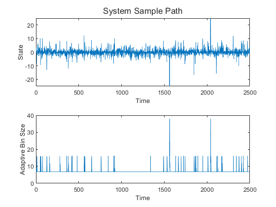
Using this scheme with the parameters above, the system was run for all and the average second moment was recorded. We remark that the settling time for the average second moment was observed to vary dramatically between small and large values of . Thus, instead of a fixed simulation length for each trial of , a variable stopping time was employed. Let
be the average second moment up to time . A small convergence threshold and an integer settling time are defined, and the simulation stops when for consecutive time stages we have . That is, the average second moment varies no more than across a single time stage for consecutive time stages. For the simulations presented here, the convergence threshold used is and the settling time is .
The second moment achieved in each trial (i.e., for each ) is plotted against the capacity below in Figure 3.
Since we expect that the optimality gap will converge to zero at a rate like for some , it is reasonable to expect that the logarithm of the optimality gap is approximately linear in with slope . Therefore, an estimate of the order of convergence was obtained by performing a linear regression between and the logarithm of the optimality gap. This estimate on the order of convergence can be seen in Figure 3. Finally, a finite segment of a sample path for the Markov chain is displayed in Figure 4 for the case .
Finally, we remark on the convergence rate to the invariant measure . In [51, Theorem IV.2] it is shown that in the scalar case with Gaussian noise, using only the adaptive part of the coding scheme, the Markov chain is “geometrically ergodic” in that for every , the -stage transition kernels converge to under the total variation metric at a rate for some .
Much of the analysis needs to be re-derived in the more general case we consider here, but one can still follow the primary line of argument in the proof of [51, Theorem IV.2]. In particular, invoking [51, Theorem III.7] with the Lyapunov function and using our super-geometric bound on the tail probabilities , Lemma 6.5, one can show that the scheme presented here also ensures that the Markov chain is geometrically ergodic for each (in this proof, which we have not worked out in detail, a careful argument is needed to ensure that the geometric rate is uniformly bounded over all ). This difficulty is of similar flavor that we resolved by a careful choice of Lyapunov parameters in Lemma 4.9).
VI Conclusion and Future Work
In conclusion, we have constructed joint coding and control schemes for networked control systems of the form (1) which are asymptotically optimal in the sense that, as the data rate grows without bound, the system second moment converges to the classical optimum with an explicit rate of convergence. The techniques in this paper build on prior work in this context, in particular by the use of random-time Lyapunov drift conditions to establish key stability results.
There are several potential directions for future work. It would be interesting to explore optimality of schemes for non-linear systems. The two-stage scheme approach seems applicable here, supposing that one can establish stability and ergodicity results by the adaptive part of the code. For instance, in [52, Theorem 5.1], a nonlinear system with “sub-linear” dynamics and additive Gaussian noise is shown to admit stability when subjected to an adaptive zooming quantization scheme similar to what is presented in [12, 13] and the adaptive stage of the scheme presented here. It seems feasible that employing a two-stage (adaptive and fixed) uniform quantization scheme for systems of this type would, by some extra analysis, lead to convergence results similar to what we have presented here.
One direction is the relaxation of the invertibility assumption on the control matrix . In general, it is possible to achieve stability in the sense of positive Harris recurrence and finite system moments with just the assumption that the pair is controllable [2, Theorem 2.2]. Controllability is a natural relaxation of the invertibility assumption to pursue for the kinds of linear systems considered here. Nonetheless, for optimality arguments on rates of decay in the distortion as the rate increases, further analysis is needed.
A further possibility is to consider stricter conditions on the noise process than Condition 4.1. For instance, one might assume that the noise tails are dominated by exponential decay (i.e., the noise has sub-exponential distribution), and seek to construct schemes which, in the sense of Definition 4.1, achieve rate functions that are much better than exponential (e.g., polynomial in ). The two-part coding scheme presented here is well suited to generalizations of this type, because the bound of Lemma 6.5 holds quite generally (e.g., with few assumptions on the noise process) and repeated use of this bound and Condition 4.1 leads to most of our key results. Thus, using this bound with a stricter condition on the noise process may lead to stronger stability and optimality results.
Appendix: Proofs
Proof of Proposition 1.1.
We show that in the fully observed setup, the optimal control policy which minimizes (2) is , achieving an optimal cost of , where is the trace operator. Let so that , then under any policy we have
| (30) | ||||
by positive definiteness of and that is i.i.d. zero-mean. In the case we have and so (30) is an equality, establishing optimality. ∎
Proof of Lemma 3.1.
Suppose that without loss of generality so that we are considering control of the following system,
across a discrete noiseless channel of capacity bits using an arbitrary joint coding and control scheme . First, note we may assume that for all sufficiently large,
| (31) |
If this fails to be true for the joint scheme then (12) will trivially hold. Note that (31) implies that
| (32) |
We will follow the core arguments in the proof of [47, Theorem 11.3.2] with the key difference of not assuming that exists.
Denote the received channel output at time as . Let , and note that the system update gives us .
We note that the discrete noiseless channel we consider is a special (noise-free discrete memoryless) case of “Class A” channels [47, Definition 8.5.1]. Such channels have their capacity characterized by limits of the directed mutual information between the channel input and output. In particular, following the beginning of the proof of [47, Theorem 8.5.2], we find that our channel capacity satisfies
| (33) |
where is the conditional mutual information. Following the analysis in the proof of [47, Theorem 11.3.2] (essentially exactly that on page 392) and invoking a conditional version of the entropy-power inequality [47, Lemma 5.3.2] we are able to arrive at the following bound,
by the convexity of . Above, and are the regular and conditional differential entropies, respectively. Therefore, we arrive at the following bound on the channel capacity in view of (33),
We will consider the two limits above separately. Let
and since we have that .
Then since is continuous and monotone decreasing in we have
Therefore, we have that
| (34) |
and what remains is to bound this limit supremum. We then have,
| (35) | ||||
| (36) |
Above, (35) follows since is constant given and differential entropy is translation invariant. (36) follows since conditioning reduces differential entropy.
We now show that .
Note that since the noise process is added to the state at every time stage and has a pdf which is positive everywhere on , the state will also have a positive-everywhere density. Furthermore, the state will also have finite variance at each time stage.
It is known that for a distribution over with specified variance , the Gaussian distribution maximizes differential entropy at . Therefore we have,
where the final limit is zero by (32).
Therefore, we have the following ultimate bound on the channel capacity,
Recall that . Rearranging the above inequality for the optimality gap we find that
which completes the proof. ∎
Proof of Lemma 4.5.
Define the event by
To start, the -th component of is . Therefore,
| (37) |
by triangle inequality and Jensen’s inequality. Since is such that for all , it follows by construction of that . Therefore,
| (38) |
Note that , then for the second expectation of (37) we have by Hölder’s inequality that
| (39) |
Recall that we suppose . It follows by Cauchy-Schwarz inequality that the expectation in (39) is bounded as
| (40) |
Note that by Markov’s inequality, we have for that
and so since , the tail probability in (39) can be bounded as,
Combining this with (39) and (40) we find that
which, combined with (38) yields that
Now that we have demonstrated that each component of satisfies the desired bound, the proof completes as follows. For any matrix we have by triangle inequality and Jensen’s inequality that
| (41) |
The proof can be completed by noting that for any two positive semidefinite matrices we have . Note that for any random vector , is positive semidefinite. Therefore, for any positive semidefinite matrix it follows that
and so the proof concludes in view of (41). ∎
We now proceed with proving stability of in the sense of both positive Harris recurrence as well as moment stability. To show positive Harris recurrence, we will need to demonstrate that our chain is irreducible and that an appropriate class of sets are small. The proofs of these two technical results (Propositions 6.1 and 6.2) are tedious and so we only provide proof sketches for brevity. For details, see [46].
Proposition 6.1.
The process is -irreducible and aperiodic, where is the product of the Lebesgue and discrete measures on .
Sketch of Proof.
The condition of aperiodicity is strictly stronger than that of irreducibility, so it suffices to show only aperiodicity. Loosely, from any initial state and a target set with there exists some such that for every , we can drive the system from to in time stages with positive probability.
The reason this is possible is that we may “hold” the bin size constant when it is less than , and so by careful management we may direct the bin size to anywhere in the state space we like (with a big enough ). In particular, we can direct the system to so long as the state falls into a subset of positive Lebesgue measure at time . That this happens with positive probability is because the state is convolved with noise at every time stage that has a positive-everywhere pdf . ∎
We denote the in-view set as
| (42) |
and in light of Section II-C we will develop results concerning the return time .
Proposition 6.2.
For the Markov chain , bounded subsets of are small.
Sketch of Proof.
We can show that subsets of containing only one bin size are -small. This follows mainly since such sets are bounded and is known deterministically, so the next-stage pdf is bounded from below by a sub-probability measure in terms of the initial set and the noise pdf .
It follows by aperiodicity that any finite union of small sets is small, and since bounded subsets of are the finite union of subsets with one bin size (which are -small), these sets are small (though generally not -small). ∎
The following proposition will prove to be remarkably useful for the remainder of our proof program.
Proposition 6.3.
Let be an i.i.d. sequence of nonnegative random variables. For any and integer we have
Proof.
Since is identically distributed, we have for that
∎
Corollary 6.4.
Let be an i.i.d. sequence of nonnegative random variables. Then for any (real) and integer we have
Proof.
Using the tail formula for expectation of a nonnegative random variable and the previous proposition, we have
∎
Lemma 6.5.
Define the constants
For we have for any that
| (43) |
Proof.
Starting from , let . We define the map by
Note that for all . The correction term accounts for the possibility that .
We construct the following ”zoom-out” process . Let , and for let
| (44) |
Then the following holds for all :
Therefore, it follows that for ,
We may further relax this event as
| (45) | ||||
| (46) | ||||
| (47) | ||||
| (48) |
Above, (45) follows by triangle inequality, (46) holds in light of (24), (47) holds since and (48) holds since .
The steps (45) through (47) can be repeated more times to ultimately obtain that the event (47) implies
| (49) |
Using the fact that and that starting in-view, , we find that
Therefore,
Note that since we have for . Therefore, so we may apply Proposition 6.3 to the sequence of i.i.d. random variables to find that
Finally, note that with we have,
which, since is nonincreasing, proves the claimed bound (43).
Corollary 6.6.
For , the in-view return time satisfies
Proof.
Note that by Condition 4.1 , we have (this follows since ). Therefore by Markov’s inequality we have for that
We use the tail formula for the expectation of a nonnegative discrete random variable and Lemma 6.5 to then find that for ,
where the series converges because each term is for . We remark that implies that the above is uniformly bounded (when one replaces by ) and that as the above is , which proves both claims. ∎
Finally, we prove positive Harris recurrence.
Proof of Theorem 4.6.
Following the remark after Condition 2.1, we will satisfy the drift condition (8) for Lemma 2.6. In this case, we set the following.
where is finite by Corollary 6.6, and is such that implies that (such a exists by Corollary 6.6). We note that is a small set by Proposition 6.2.
First, notice that by construction we have for any that , so the second inequality of (8) is satisfied. We now show that the first inequality also holds, which in this case is that for any ,
| (51) |
First, note that for we have that , so,
Thus we have that
| (52) |
First, suppose (so that ), then by construction of and , (52) becomes
which satisfies (51). Next, suppose that , then by construction of and , (52) becomes
and so (51) is satisfied over . It follows then by Lemma 2.6 that is positive Harris recurrent, provided that we can show that for all . We do this to complete the proof.
Since we have proven the drift condition (8) holds at all , it follows from the proof of Lemma 2.6 that for all we have
so we must have that for all . From here, it suffices to verify that all states return to in finite time. This is automatic for initial by Corollary 6.6. Now suppose that . By nearly identical arguments to those of Lemma 6.5, we can show that
For sufficiently large we have , so we may apply Proposition 6.3 which yields that for sufficiently large,
which converges to zero as grows large (, as in the proof of Corollary 6.6). Therefore, we must have , which completes the proof. ∎
Proof of Proposition 4.7.
To complete the proof program, we must show the moment condition of Lemma 4.9 holds. The rest of the Appendix is dedicated to this proof. We first have some intermediate results.
Proposition 6.7.
Under Scheme P, for the return time satisfies the following independently of .
Proof.
Note that by Condition 4.1 with and Markov’s inequality we have for that
Let for brevity. Then we have by Lemma 6.5 that
Above, the series converges since the summand is , where (this is ensured by the assumption that . Then, we have shown that
which (in light of the fact that ) completes the proof. ∎
Proposition 6.8.
Under Scheme P, the invariant state has finite -th moment uniformly in . That is,
Proposition 6.9.
Under Scheme P, the invariant adaptive bin size has finite -th moment uniformly in . That is,
We will prove these two results shortly via Lyapunov drift arguments, but using them we will first provide a short proof of Lemma 4.9.
Proof of Lemma 4.9.
Let and let . It follows that is distributed as the invariant system adaptive error. Note that for any we have the inequality , where the extra term accounts for the possibility that . Therefore, we have that
and so,
| (54) |
Above, the second bound follows from the general fact that for any and nonnegative random variables we have
| (55) |
which follows by convexity of when (via Jensen’s inequality) and by sub-additivity of when .
All that remains is to prove Propositions 6.8 and 6.9, which we do here via Lyapunov drift arguments.
Proof of Proposition 6.8.
Recall that we must show that
We will do this via random-time Lyapunov drift arguments, in particular Lemma 2.7 using the drift condition (8). Let as in Proposition 6.7. We set the following:
where is arbitrary, is such that
(such a exists by Proposition 6.7), is finite by Proposition 6.7, and is a sufficiently small constant (which will be specified shortly). We will show that the drift condition (8) holds for the choices above.
First, note that for we have that , so
| (56) |
For , by construction of we have that (56) is bounded by . For , by construction of we have that (56) is nonpositive. In either case, the first drift inequality is satisfied.
Next we show that the second inequality of (8) holds, when is sufficiently small. To start, we have that for that
| (57) |
The remainder of the proof will be dedicated to showing that there exists a constant so that uniformly over we have,
| (58) |
so that we may bound (57) as
| (57) |
It then suffices to take , and the second drift inequality holds. Therefore, we dedicate the remainder of this proof to establishing (58).
As in the proof of Lemma 6.5, the “zoom-out” process defined by , agrees with for . Therefore, we have that
| (59) |
where the exchange of summation and expectation is justified by the monotone convergence theorem [43, Theorem 1.26].
Let for brevity. Now, choose arbitrarily (this is a valid interval by the condition that ). We let be the Hölder conjugate of (i.e., ) and apply Hölder’s inequality to (59).
| (60) |
We will consider each factor of the summand separately. First, by Lemma 6.5 and familiar arguments we have
so that for series convergence,
| (61) |
and this term is . Next, we consider the second summand factor of (60). For brevity, let . Since and , we have for that
Repeating this argument times yields
and since and we find that
Therefore, we have by Corollary 6.4 and repeated application of (55) that
where implies that . Note that the term is . Then finally we have,
| (62) |
which in combination with (61) yields that (60) is bounded by
where the series above converges to a constant when . This is ensured by the condition , since then we have
This establishes (58) and completes the proof. ∎
Proof of Proposition 6.9.
Recall that we must show that
We will do this again via random-time Lyapunov drift arguments. In particular, we will use most of the same Lyapunov parameters as in the previous proof. To be precise, with we once again set
where is arbitrary, is such that
(such a exists by Proposition 6.7), and is finite by Proposition 6.7.
Instead of proportional to , we set proportional to . That is, we set:
where
is well-defined by Proposition 6.7. We will show that these Lyapunov parameters satisfy the drift condition (8) and invoke Lemma 2.7 to complete the proof.
To begin, note that the first drift inequality of (8) does not involve , and with otherwise identical Lyapunov parameters we showed in the proof of Proposition 6.8 that this drift inequality holds. Therefore, what remains is to show only that the second inequality in (8) holds. Explicitly, we must show that
which is equivalent to,
| (63) |
We establish this now. Note that and for we have so,
by construction of . Therefore the drift condition (8) is satisfied for choice of and independent of , which by Lemma 2.7 completes the proof. ∎
References
- [1] J. Keeler, T. Linder, and S. Yüksel, “An asymptotically optimal two-part coding scheme for networked control under fixed-rate constraints,” IEEE International Symposium on Information Theory, ISIT, 2022.
- [2] A. Johnston and S. Yüksel, “Stochastic stabilization of partially observed and multi-sensor systems driven by unbounded noise under fixed-rate information constraints,” IEEE Transactions Automatic Control, vol. 59, pp. 792–798, March 2014.
- [3] D. Bertsekas, Dynamic Programming and Optimal Control Vol. 1. Athena Scientific, 2005.
- [4] W. S. Wong and R. W. Brockett, “Systems with finite communication bandwidth constraints - part II : Stabilization with limited information feedback,” IEEE Transactions on Automatic Control, vol. 42, pp. 1294–1299, September 1997.
- [5] J. Baillieul, “Feedback designs for controlling device arrays with communication channel bandwidth constraints,” in Proceedings of the 4th ARO Workshop on Smart Structures, State College, PA, August 1999.
- [6] S. Tatikonda and S. Mitter, “Control under communication constraints,” IEEE Transactions on Automatic Control, vol. 49, no. 7, pp. 1056–1068, 2004.
- [7] L. V. J. Hespanha, A. Ortega, “Towards the control of linear systems with minimum bit-rate,” in Proc. 15th Int. Symp. on Mathematical Theory of Networks and Systems (MTNS), 2002.
- [8] G. N. Nair and R. J. Evans, “Stabilizability of stochastic linear systems with finite feedback data rates,” SIAM J. Control and Optimization, vol. 43, pp. 413–436, July 2004.
- [9] A. Sahai and S. Mitter, “The necessity and sufficiency of anytime capacity for stabilization of a linear system over a noisy communication link part I: Scalar systems,” IEEE Transactions on Information Theory, vol. 52, no. 8, pp. 3369–3395, 2006.
- [10] N. C. Martins, M. A. Dahleh, and N. Elia, “Feedback stabilization of uncertain systems in the presence of a direct link,” IEEE Transactions on Automatic Control, vol. 51, no. 3, pp. 438–447, 2006.
- [11] A. S. Matveev and A. Savkin, “An analogue of Shannon information theory for detection and stabilization via noisy discrete communication channels,” SIAM J. Control Optim, vol. 46, pp. 1323–1367, 2007.
- [12] S. Yüksel, “Stochastic stabilization of noisy linear systems with fixed-rate limited feedback,” IEEE Transactions on Automatic Control, vol. 55, pp. 2847–2853, December 2010.
- [13] S. Yüksel and S. P. Meyn, “Random-time, state-dependent stochastic drift for Markov chains and application to stochastic stabilization over erasure channels,” IEEE Transactions on Automatic Control, vol. 58, pp. 47 – 59, January 2013.
- [14] V. Kostina, Y. Peres, G. Ranade, and M. Sellke, “Exact minimum number of bits to stabilize a linear system,” IEEE Transactions on Automatic Control, vol. 67, no. 10, pp. 5548–5554, 2022.
- [15] O. Sabag, V. Kostina, and B. Hassibi, “Stabilizing dynamical systems with fixed-rate feedback using constrained quantizers,” in 2020 IEEE International Symposium on Information Theory (ISIT). IEEE, 2020, pp. 2855–2860.
- [16] R. Zamir and M. Feder, “On universal quantization by randomized uniform/lattice quantizers,” IEEE Transactions on Information Theory, vol. 38, no. 2, pp. 428–436, 1992.
- [17] E. I. Silva, M. S. Derpich, and J. Østergaard, “A framework for control system design subject to average data-rate constraints,” IEEE Transactions on Automatic Control, vol. 56, pp. 1886–1899, August 2011.
- [18] C. D. Charalambous, P. A. Stavrou, and N. U. Ahmed, “Nonanticipative rate distortion function and relations to filtering theory,” IEEE Transactions on Automatic Control, vol. 59, no. 4, pp. 937–952, 2014.
- [19] V. Kostina, “Data compression with low distortion and finite blocklength,” IEEE Transactions on Information Theory, vol. 63, no. 7, pp. 4268–4285, 2017.
- [20] V. Kostina and B. Hassibi, “Rate-cost tradeoffs in control,” IEEE Transactions on Automatic Control, vol. 64, no. 11, pp. 4525–4540, 2019.
- [21] J. Østergaard, “Stabilizing error correction codes for controlling LTI systems over erasure channels,” in IEEE Conference on Decision and Control (CDC), 2021.
- [22] E. Silva, M. Derpich, J. Østergaard, and M. Encina, “A characterization of the minimal average data rate that guarantees a given closed-loop performance level,” IEEE Transactions on Automatic Control, vol. 61, no. 8, pp. 2171–2186, 2015.
- [23] P. Stavrou, J. Østergaard, and C. Charalambous, “Zero-delay rate distortion via filtering for vector-valued Gaussian sources,” IEEE Journal of Selected Topics in Signal Processing, vol. 12, no. 5, pp. 841–856, 2018.
- [24] T. Cuvelier, T. Tanaka, and R. W. Heath Jr., “Time-invariant prefix coding for LQG control,” arXiv preprint arXiv:2204.00588, 2022.
- [25] J. L. Massey, “Causality, feedback and directed information,” in IEEE International Symposium on Information Theory, Waikiki, Hawaii, 1990, pp. 303–305.
- [26] A. Gorbunov and M. Pinsker, “Nonanticipatory and prognostic epsilon entropies and message generation rates,” Problemy Peredachi Informatsii, vol. 9, no. 3, pp. 12–21, 1973.
- [27] R. Bansal and T. Başar, “Simultaneous design of measurement and control strategies in stochastic systems with feedback,” Automatica, vol. 45, pp. 679–694, September 1989.
- [28] S. Tatikonda, A. Sahai, and S. Mitter, “Stochastic linear control over a communication channels,” IEEE Transactions on Automatic Control, vol. 49, pp. 1549–1561, September 2004.
- [29] T. Tanaka, “Semidefinite representation of sequential rate-distortion function for stationary Gauss-Markov processes,” in 2015 IEEE Conference on Control Applications (CCA). IEEE, 2015, pp. 1217–1222.
- [30] T. Tanaka, K. Kim, P. Parrilo, and S. Mitter, “Semidefinite programming approach to Gaussian sequential rate-distortion trade-offs,” IEEE Transactions on Automatic Control, vol. 62, no. 4, pp. 1896–1910, 2016.
- [31] T. Tanaka, P. M. Esfahani, and S. K. Mitter, “LQG control with minimum directed information: Semidefinite programming approach,” IEEE Transactions on Automatic Control, vol. 63, no. 1, pp. 37–52, 2018.
- [32] M. Derpich and J. Østergaard, “Improved upper bounds to the causal quadratic rate-distortion function for Gaussian stationary sources,” IEEE Transactions on Information Theory, vol. 58, no. 5, pp. 3131–3152, 2012.
- [33] P. Stavrou, T. Charalambous, C. Charalambous, and S. Loyka, “Optimal estimation via nonanticipative rate distortion function and applications to time-varying Gauss–Markov processes,” SIAM Journal on Control and Optimization, vol. 56, no. 5, pp. 3731–3765, 2018.
- [34] P. Stavrou and M. Skoglund, “Asymptotic reverse waterfilling algorithm of NRDF for certain classes of vector Gauss-Markov processes,” IEEE Transactions on Automatic Control, vol. 67, no. 6, pp. 3196–3203, 2022.
- [35] P. Stavrou, T. Tanaka, and S. Tatikonda, “The time-invariant multidimensional Gaussian sequential rate-distortion problem revisited,” IEEE Transactions on Automatic Control, vol. 65, no. 5, pp. 2245–2249, 2019.
- [36] S. Yüksel, “Jointly optimal LQG quantization and control policies for multi-dimensional linear Gaussian sources,” IEEE Transactions on Automatic Control, vol. 59, pp. 1612–1617, June 2014.
- [37] ——, “A note on the separation of optimal quantization and control policies in networked control,” SIAM Journal on Control and Optimization, vol. 57, no. 1, pp. 773–782, 2019.
- [38] T. Linder and S. Yüksel, “On optimal zero-delay quantization of vector Markov sources,” IEEE Transactions on Information Theory, vol. 60, pp. 2975–5991, October 2014.
- [39] M. Ghomi, T. Linder, and S. Yüksel, “Zero-delay lossy coding of linear vector Markov sources: Optimality of stationary codes and near optimality of finite memory codes,” IEEE Transactions on Information Theory, vol. 68, no. 5, pp. 3474–3488, 2021.
- [40] B.-H. Juang and A. Gray, “Multiple stage vector quantization for speech coding,” in ICASSP ’82. IEEE International Conference on Acoustics, Speech, and Signal Processing, 1982.
- [41] T. Berger, “Information rates of Wiener processes,” IEEE Transactions on Information Theory, vol. 16, pp. 134–139, 1970.
- [42] A. Sahai, “Coding unstable scalar Markov processes into two streams,” in Proceedings of the IEEE International Symposium on Information Theory, 2004.
- [43] W. Rudin, Real and Complex Analysis, 3rd ed. McGraw-Hill Book Company, 1987.
- [44] E. Nummelin, “A splitting technique for Harris recurrent Markov chains,” Z. Wahrscheinlichkeitstheoric verw. Gebiete, vol. 43, pp. 309–318, 1978.
- [45] K. B. Athreya and P. Ney, “A new approach to the limit theory of recurrent Markov chains,” Transactions of the American Mathematical Society, vol. 245, pp. 493–501, 1978.
- [46] J. Keeler, “An Asymptotically Optimal Two-Part Fixed-Rate Coding Scheme for Networked Control,” Master’s thesis, Queen’s University, 2022.
- [47] S. Yüksel and T. Başar, Stochastic Networked Control Systems: Stabilization and Optimization under Information Constraints. New York: Springer, 2013.
- [48] D. Hui and D. Neuhoff, “Asymptotic analysis of optimal fixed-rate uniform scalar quantization,” IEEE Transactions on Information Theory, vol. 47, no. 3, pp. 957–977, 2001.
- [49] C. Kawan and S. Yüksel, “Metric and topological entropy bounds for optimal coding of stochastic dynamical systems,” IEEE Transactions on Automatic Control, vol. 65, no. 6, pp. 2466–2479, 2020.
- [50] R. A. Horn and C. R. Johnson, Matrix Analysis, 2nd ed. Cambridge University Press, 2013.
- [51] R. Zurkowski, S. Yüksel, and T. Linder, “On rates of convergence for Markov chains under random time state-dependent stochastic drift criteria,” IEEE Transactions on Automatic Control, vol. 61, no. 1, pp. 145–155, 2015.
- [52] S. Yüksel, “Stationary and ergodic properties of stochastic non-linear systems controlled over communication channels,” SIAM J. on Control and Optimization, vol. 54, pp. 2844–2871, 2016.