Learning to be a Statistician: Learned Estimator for Number of Distinct Values
Abstract.
Estimating the number of distinct values (NDV) in a column is useful for many tasks in database systems, such as columnstore compression and data profiling. In this work, we focus on how to derive accurate NDV estimations from random (online/offline) samples. Such efficient estimation is critical for tasks where it is prohibitive to scan the data even once. Existing sample-based estimators typically rely on heuristics or assumptions and do not have robust performance across different datasets as the assumptions on data can easily break. On the other hand, deriving an estimator from a principled formulation such as maximum likelihood estimation is very challenging due to the complex structure of the formulation. We propose to formulate the NDV estimation task in a supervised learning framework, and aim to learn a model as the estimator. To this end, we need to answer several questions: i) how to make the learned model workload agnostic; ii) how to obtain training data; iii) how to perform model training. We derive conditions of the learning framework under which the learned model is workload agnostic, in the sense that the model/estimator can be trained with synthetically generated training data, and then deployed into any data warehouse simply as, e.g., user-defined functions (UDFs), to offer efficient (within microseconds on CPU) and accurate NDV estimations for unseen tables and workloads. We compare the learned estimator with the state-of-the-art sample-based estimators on nine real-world datasets to demonstrate its superior estimation accuracy. We publish our code for training data generation, model training, and the learned estimator online for reproducibility.
PVLDB Reference Format:
Renzhi Wu,
Bolin Ding,
Xu Chu,
Zhewei Wei,
Xiening Dai,
Tao Guan,
Jingren Zhou. PVLDB, 15(2): 272 - 284, 2022.
doi:10.14778/3489496.3489508
††
This work is licensed under the Creative Commons BY-NC-ND 4.0 International License. Visit https://creativecommons.org/licenses/by-nc-nd/4.0/ to view a copy of this license. For any use beyond those covered by this license, obtain permission by emailing info@vldb.org. Copyright is held by the owner/author(s). Publication rights licensed to the VLDB Endowment.
Proceedings of the VLDB Endowment, Vol. 15, No. 2 ISSN 2150-8097.
doi:10.14778/3489496.3489508
1. Introduction
Estimating number of distinct values (NDV), also known as cardinality estimation, is a fundamental problem with numerous applications (Harmouch and Naumann 2017; Haas et al. 1995; Nath et al. 2008; Mohamadi et al. 2017). It has been extensively studied in many research communities including databases (Haas et al. 1995; Charikar et al. 2000), networks (Nath et al. 2008; Cohen and Nezri 2019), bioinformatics (Mohamadi et al. 2017), and statistics (Bunge and Fitzpatrick 1993; Haas and Stokes 1998; Pavlichin et al. 2019).
The methods for estimating NDV in the absence of an index can be classified into two categories: sketch based methods and sampling based methods (Metwally et al. 2008). Sketch based methods scan the entire dataset once, followed by sorting/hashing rows, and create a sketch that is used to estimate NDV (Harmouch and Naumann 2017). Sampling based methods estimate NDV using statistics from a small sample, without needing to scan the entire dataset. Generally, sketch based methods give more accurate estimation, but scanning and hashing the entire dataset can be prohibitively expensive in large data warehouses. Hashing techniques such as probabilistic counting help alleviate the memory requirements but still requires a full scan of the table. When a full scan is not possible or the computation cost of a full scan is not affordable, sampling based methods are the only remaining alternatives which exam only a very small fraction of the table, i.e., a sample, and thus scale well with increasing data set.
In this paper, we focus on the problem of accurately estimating the number of distinct values from samples of large tables.
The first challenge is that, unlike some other statistical parameters, such as means and histograms, which can be accurately computed from small random samples, accurate NDV estimation from small samples has been proved to be an extremely difficult task (e.g., with theoretical lower bounds of error given in (Charikar et al. 2000)).
We can formulate sample-based NDV estimation using a principled method for estimating unknown parameters, the maximum likelihood estimation (MLE) (Chambers et al. 2012). An MLE estimator is workload-agnostic: it is derived (analytically) before we see the real workloads. It solves an optimization problem, which maximizes the likelihood of observing a specific random sample, and gives an NDV estimation with desirable properties such as consistency and efficiency. However, the remaining steps are challenging (if not impossible): how to express the likelihood function and the optimization problem in a compact way, and how to (even approximately) solve it.
Due to the above challenges, this paper proposes and studies a more fundamental question: whether it is possible to train a workload-agnostic machine learning model to approximate principled statistical estimators such as MLE estimators, with the training set synthetically generated from a training distribution calibrated based on the properties of our estimation task, such that the learned model can be used on unseen workloads.

Learning to be a Statistician: a Toy Example
It is traditionally the statistician’s job to derive a closed-form or numerical estimator as a function that takes an observed sample or sample statistics as the input for estimating unknown parameters of a statistical model. On the other hand, it is known that any continuous function can be approximated by a neural network (with enough nodes and layers) (Haykin 1998), which require three elements: a training set , a class of model architectures , and a training algorithm. Thus, a natural question is whether we can train a neural network in a workload-agnostic way (without seeing any real dataset during training) to approximate, e.g., an MLE estimator. Following are two examples with positive answers to this question.
Learning MLE of mean and STD. Let’s consider the mean and standard deviation (STD) of a Gaussian distribution. For a size- sample drawn from this distribution, , the MLE estimations of and are known to have closed forms: and , respectively. Assume that we do not know the concrete form of and . How should we train machine learning models to approximate them?
We first need to prepare the training data. From a specific Gaussian distribution , we draw a size- sample , and add one training data point to the training set for mean estimation, and one data point to for STD estimation. Note that, here, each is a -dim feature vector, and each and are the (ground-truth) labels to be predicted for mean and STD, respectively. In the outer loop, we need to try different combinations of and to add more training data points into and . In this example, we generate pairs of , where each is randomly picked from a Gaussian distribution and each is picked from a folded Gaussian distribution (i.e., where ). Thus, we will have training data points in each of and .
We train a regression model (multi-layer perception with one hidden layer of size and mean squared loss) using the training set for estimating and another model (with the same architecture) on for estimating , both with as feature.
We evaluate the trained estimator on a completely different test set. We generate pairs with each and from uniform distributions. For each , we generate a test data point and a point for a size- sample from . The results are reported in Figure 1 (where we use ). Figures 1(1)-(2) show that the estimations of mean/STD given by the trained model have very similar performance as those by the closed-form MLE estimations. The trained model and MLE even make the same mistakes for some test points with non-trivial errors. Figure 1(3) compares and the learned estimator on more data points for STD estimation, for which the MLE estimator has a more complex form than a linear model for the mean estimation.
Our Contributions and Solution Overview
In this paper, we will formalize and investigate the learning framework illustrated in the above example, but for a more challenging task, sample-based NDV estimation. While the empirical evidence for mean/STD estimation sheds light on the possibility of approximating MLE estimators with trained models, there are several key questions to be resolved for general estimation tasks: i) how to generate training data and what features should be extracted for learning the model; ii) what model architecture, loss function, and regularization should be used; iii) with the choice in i) and ii), whether the trained estimator approximates MLE and performs in a robust and workload-agnostic way.
MLE formulation. We first formulate NDV estimation as an MLE problem. Assuming that a data column is generated from some prior distribution and a sample is drawn uniformly at random from the column, we observe the sample profile, i.e., a vector where is the number of distinct values with frequency in . For example, for , we have , (‘’ has frequency ), and (‘’ and ‘’). For an MLE estimation, we aim to find the value of NDV, , such that the probability of observing conditioned on is maximized. Although it is difficult to solve (even approximately) the MLE formulation, it will guide the design and analysis of our machine learning model.
Learning estimator that approximates MLE. With the sample profile as a feature and the ratio error between the estimate and the true NDV as the training loss, we have a skeleton of the learning framework. Unlike learning MLE for mean and STD where the training data preparation is trivial because each dimension of the feature space ( in ) can be independently generated, in NDV estimation, however, different dimensions of the sample profile ( in ) are correlated, conditioned on NDV; thus, it is more difficult to characterize the distribution needed for preparing the training set. After carefully investigating the probability distribution the model learns based on our choice of feature and loss and comparing the learned probability distribution with the one in our MLE formulation, we derive several precise properties to characterize the training distribution we need in order to make the learned estimator approximate an MLE estimator.
Efficient training data generation. We design an efficient algorithm to generate training data points. To generate one data point, we need to first generate a data column (in a compact way). And instead of drawing a sample explicitly, we directly generate the sample profile from its distribution determined by the data column. In our experiment, - data points suffice to train the estimator.
Instance-wise negative results and model regularization. It is important to note that the negative result about sample-based NDV estimation in (Charikar et al. 2000) also hold for “learned estimators”. However, the negative result in (Charikar et al. 2000) is a global one, in the sense that there exist hard instances of data columns whose NDVs are difficult to be estimated. However, the hope is that, upon the observation of the sample profile, it is possible to infer that the underlying data column is not a hard instance and an estimate with error lower than the global lower bound can be expected. We first derive a new instance-wise negative result, i.e., a lower bound of the estimation error upon the observation of a sample profile. We use this negative result to regularize the training of our model. More specifically, we propose a regularization method that encourages the learned estimator to achieve just the instance-wise lower bound of estimation error, instead of always minimizing the estimation error to be zero (which is an impossible goal due to global negative result). Its effectiveness will be verified via experimental studies.
Deployment and experiments. The learned estimator, once trained, can be deployed in any data warehouse without the need of re-training or tuning. We publish our estimator online (Library 2021) as a trained neural network that takes a sample/sample profile of a column as the input feature and outputs an estimated NDV of that column. It is compared with the state-of-the-art sample-based NDV estimators and is shown to outperform them on nine different real datasets. Note, again, that none of these datasets is used to train our estimator, and all the training data is generated synthetically.
Related Work
Learned cardinality estimation. There have been a long line of existing works on learning a model to estimate cardinality or selectivity of a query (Anagnostopoulos and Triantafillou 2015; Lakshmi and Zhou 1998; Liu et al. 2015; Dutt et al. 2019; Kipf et al. 2018; Dutt et al. 2020; Zhu et al. 2021). In general, they can be divided into two types (Wang et al. 2021). The first type uses query as the primary feature and training data comes from the records of query executions. For example, (Dutt et al. 2019) uses query as features and applies tree-based ensembles to learn the selectivity of multi-dimensional range predicates. This type of method typically requires executing a huge number of queries to obtain enough training data (Wang et al. 2021). There are efforts to alleviate this issue: (Dutt et al. 2020) proposes to reduce model construction cost by incrementally generating training data and using approximate selectivity label. Generally, this type of methods work well when future queries follow the same distribution and similar templates (e.g., conjunction of range and categorical predicates) as the training data (Zhu et al. 2021). The second type (for example (Hilprecht et al. 2020) and (Zhu et al. 2021)) builds a model to approximate the joint distribution of all attributes in a table. This type of methods require re-training in case of data or schema update. In dynamic environments with unseen datasets and workloads coming, both type of methods require huge efforts of accessing the new dataset and retraining (Wang et al. 2021).
Although we also learn a model to estimate NDV/cardinality, our method is completely different from the above methods. Our method is a sample-based approach and we use features from sample rows (drawn from tables or query results) instead of queries. More importantly, our method is workload agnostic (only needing to be trained once) and can be applied to any dynamic workload.
Sample-based NDV estimation. Existing sampling based methods are typically constructed based on heuristics or derived by making certain assumptions. For example, there are estimators derived by assuming infinite population size (Chao and Lee 1992), certain condition of skewness (Shlosser 1981), and certain distribution of the data (Motwani and Vassilvitskii 2006). GEE estimator (Charikar et al. 2000) is constructed to match a (worst-case) lower bound of estimation error in (Charikar et al. 2000). We discuss these existing approaches in more details in Section 2.2. These approaches are not robust especially on datasets where their assumptions about data distribution break, as we will show in experiments in Section 6.
Sketch-based NDV estimation. Sketch-based methods (e.g., Hyperloglog (Flajolet et al. 2007)) scan the entire dataset once and keep a memory-efficient sketch that is used to estimate NDV. These methods are able to produce highly accurate NDV estimation. For example, the expected relative error of HyperLogLog (Flajolet et al. 2007) is about , where is the number of bytes used in HyperLogLog; With 10K bytes, the relative error of NDV estimation can be as small as -. See survey (Harmouch and Naumann 2017) for a comprehensive review.
Sample v.s. Sketch. When one scan of the data is affordable, sketch-based estimators are preferable to sample-based ones. In scenarios where a full scan of the data is (relatively) too expensive, sample-based methods are preferable. For example, when NDV estimation in a column is used by the query optimizer to generate a good execution plan for a SQL query, a high-quality sample-based estimation is preferable, as the query is almost processed after a full scan. Another example is approximate query processing (Chaudhuri et al. 2017), where offline samples are used to provide approximate answers to analytical (e.g., NDV) queries over voluminous data with interactive speed. In short, sketch-based estimators and sample-based methods are two orthogonal lines of research with different applications.
Paper Organization
In Section 2, we provide the preliminaries including an MLE-based formulation for NDV estimation, and review some representative estimators. In Section 3, we provide an overview of our learning-to-estimate framework; we analyze and derive properties of the training distribution needed to make the learned model approximate MLE. In Section 4, we give details about training data generation and model architecture; we also introduce our new instance-wise negative result about sample-based NDV estimation, and how to regularize the model accordingly. Section 5 gives a brief introduction on how to use our learned estimator that is available online. We evaluate our estimator and compare it with the state of the arts experimentally and report the results in Section 6.
2. Preliminaries
We focus on a specific data column of a table with rows. is called the population size. Let be the number of distinct values (NDV) in . When calculating NDV of the column , we consider as a (multi)set of values from some (possibly infinite) domain .
Problem statement: estimating NDV from samples. We want to estimate from a random sample of tuples drawn uniformly at random from . Let be the sampling rate. We assume , or equivalently , is observed.
We first formally define two important notations.
Frequency. The frequency of a value in a column , or a sample , is the number of times it appears in , or , denoted as , or , respectively. By definitions, we have and , and the NDV in is .
Profile. In order to calculate NDV, it is sufficient to consider the profile of , denoted as , where is the number of distinct values with frequency in ; similarly, the profile of a random sample is where is the number of distinct values with frequency in . By definitions, the NDV in is and the population size is ; The NDV in sample is and the sample size is .
2.1. An MLE-based Formulation.
Estimating NDV from random samples can be formulated as a maximum likelihood estimation (MLE) problem, which is commonly used to estimate unknown parameters of a statistical model, with desirable properties such as consistency and efficiency (Chambers et al. 2012). The estimated value (or the solution to an MLE problem) maximizes the probability of the observed data generated from this model.
We assume that the column with profile is drawn from some prior probability distribution. A uniformly random sample with profile is then drawn from . An MLE-based formulation for NDV estimation can be derived based on the observed profile in the sample , i.e., the sample profile , and the observed population size (or equivalently, sampling rate ). We estimate as the one that maximizes the probability of observing and .
Define to be all the feasible profile configurations with NDV equal to and population size equal to . For , we have ; and for , we have and . The above formulation can be rewritten as:
The estimator is to be used on unknown columns; so in order to solve the above optimization problem, it is reasonable to assume that the prior distribution of is uniform, in the sense that every possible profile in appears with equal probability, i.e., for every . Under this assumption, we want to solve the following one for :
| (1) |
We can also interpret the MLE-based formulation (1) as follows. After observing the sample profile and the population size , we estimate as which maximizes the average probability of generating from a feasible profile . Solving (1), however, is difficult even approximately, and thus this formulation has not been applied for estimating NDV yet.
A natural question is whether it benefits to use sample , instead of sample profile , as observed data to derive MLE and as features in our learning framework. We provide a formal analysis on why using sample is not more advantageous in Appendix 8.1. In fact, most existing estimators (as we show next) also use sample profile instead of sample to estimate NDV.
2.2. Existing Estimators
There have been a long line of works on estimating NDV from random samples. We review some representative ones as follows.
- •
A problem related to the one in (1) is profile maximum likelihood estimation (PML) (Hao and Orlitsky 2019; Pavlichin et al. 2019; Charikar et al. 2019), which chooses that maximizes the probability of observing of the randomly drawn . Define:
(2) There have been works on finding approximations to (Pavlichin et al. 2019; Charikar et al. 2019), which can be in turn used to obtain an approximate version of in (2), although, in general, .
- •
Shlosser (Shlosser 1981) is derived based on an assumption about skewness: , and performs well when each distinct value appear approximately one time on average (Haas et al. 1995). It estimates as
(3) - •
Chao (Chao 1984) approximates the expected NDV, , in large population for some underlying distribution, and estimates NDV as a lower bound of with the population size approaching infinity:
(4) - •
GEE (Charikar et al. 2000) is constructed by using geometric mean to balance the two extreme cases for values appearing exactly once in the sample: those with frequency one in and drawn into with probability v.s. those with high frequency in and at least one copy drawn into . It is proved to match a theoretical lower bound of ratio error for NDV estimation within a constant factor.
(5) HYBGEE (Charikar et al. 2000) is a hybrid estimator using GEE for high-skew data and using the smoothed jackknife estimator for low-skew data. AE (Charikar et al. 2000) is a more principled version of HYBGEE with smooth transition from low-skew data to high-skew data. It requires to solve a non-linear equation using, e.g., Brent’s method (bre 2020).
2.3. Negative Results
The aforementioned lower bound of ratio error for sample-based NDV estimators is given by Charikar et al. in (Charikar et al. 2000). More formally, define the ratio error of an estimation w.r.t. the true NDV to be
| (6) |
It considers in (Charikar et al. 2000) a even larger class of estimators which randomly and adaptively examine tuples from . Note that drawing a random sample of tuples is a special case here. It says that for any such estimator, there exists a choice of column such that, with probability at least , the ratio error is at least
| (7) |
3. Overview of Learning Framework
Since analytically solving (1) even approximately is difficult, we propose to formulate the task of deriving as a supervised learning problem. We first introduce some key elements in the learning model, including the loss function and the design of training dataset, which learns an estimator to approximate (1).
Learning to estimate
In typical traditional estimators such as (3)-(5), the NDV is estimated as a function of the sample profile and the sampling rate , or equivalently a function of and the population size as . As it is difficult to directly derive the function from a principled formulation such as MLE in (1), we attempt to learn the MLE of NDV from a set of training data points , where in each point, is the input feature and the NDV is the label to be predicted. We use the ratio error defined in (6) to measure the accuracy of estimations, and accordingly, the loss function of the model is:
| (8) |
Given a hypothesis set of estimation functions, the goal is to find with small empirical loss:
| (9) |
In order to generate a data point in the training set , we first generate a data column with profile according to a training distribution . The NDV as well as population size is directly calculated from . A random sample is drawn uniformly at random from with sampling rate . The sample profile is then obtained from . The above process is repeated independently multiple times to generate a training set . We only generate one sample profile from a profile to ensure that each training data point in is independently and identically distributed.
Approximating MLE
Intuitively, for a different training distribution , a different learned estimator will be derived from the hypothesis set (model architecture) . Assuming that is expressive enough (Raghu et al. 2017), we give some guidelines here on how to choose so that the learned approximates the MLE estimator .
Let denote the joint distribution of in the training set that is generated from the training distribution as above. Using the loss function in (8)-(9), i.e., the L2 loss on , the trained model learns the distribution (Goodfellow et al. 2017). By minimizing (9), the model tends to emit an output
| (10) |
for a given input . The approximation sign is because the trained model might not be able to learn the underlying distribution of the training set exactly and the accuracy of the approximation is also determined by the hypothesis set and the training algorithm. For the term on the right hand side,
| (11) |
where both equations are from properties of conditional probability.
Consider the following two conditions about the distribution :
| (12) | ||||
| (13) |
Namely, i) for any fixed , the NDV distributes uniformly at log scale (or equivalently distributes uniformly) in ; and ii) for any fixed and , every feasible profile appears with equal probability. If both are satisfied, the maximizer of (11) (as a function of ) can be written as
| (14) |
by putting (12)-(13) back into (11). The second equality in (14) is because is a probability term that is independent on ; and the last equality is from the definition of in (1). Therefore, the learned estimator approximates if the training distribution satisfies the two conditions in (12)-(13).
From the above analysis, the learned estimator approximates (14) which depends on only and : the former is a deterministic finite set, and the latter is a probability distribution depending only on the sampling procedure but not on ; therefore, intuitively, we can expect that is workload-agnostic, i.e., it generalizes well on unseen data columns, which will be verified later in our experiments reported in Section 6.
About uniformity of . When introducing the MLE estimator and analyzing its equivalence to the learned model , the underlying assumption is that the prior distribution of is uniform. In fact, any targeted prior distribution of can be plugged into and accordingly, used as the training distribution for . However, we assume the uniformity purposely to enable the learned estimator generalize to unseen datasets (workload-agnostic). We tried to train an estimator (Lower Bound (LB) in Section 6) with the prior of and the same as those in the test datasets. In experiments, we observed that the LB estimator works well only on this particular workload but does not generalize to unseen workloads. In comparison to the LB estimator with the “optimal” prior, our workload-agnostic estimator with the uniform prior has comparable performance on every test table (refer to, e.g., Table 2).
4. Learning Estimator from Data
4.1. Efficient Training Data Generation
As long as the training data satisfies the conditions in (12)-(13), whether the data is synthetic or from real world makes no difference. This makes it possible for us to train the model using synthetically generated data without needing any real-world data.
To generate a training data point , one may first generate a random column , then draw a random sample from and calculate sample profile from . However, since the population profile of contains all required information to generate a random sample profile (as we will show in Section 4.1.2), we can directly randomly generate a population profile and then draw a random sample profile from .
4.1.1. Population profile generation
Generating population profile is to draw samples from the distribution , written as:
| (15) |
We can draw samples from by repeating the following: sample a from , sample a from , and sample a from , with and satisfying the conditions in (12)-(13). In order to ensure the training data to be diverse, we want to have cover a big range of magnitude, so we set the distribution of to be uniform at log scale, i.e., where is a constant specifying the maximum population size. We select according to the memory limit of our machine.
Generating from is, however, non-trivial. Given population size and population NDV , drawing a population profile from is equivalent to randomly sampling an element under i) the uniform-distribution constraint (i.e., every feasible has equal probability to be drawn) from set which is specified by the two constraints ii) and iii) . Designing such a sampling procedure that satisfies the three constraints simultaneously is very challenging.

If the dimensionality of can be given, the sampling procedure is easier. Consider an alternative form of :
| (16) |
This indicates an alternative procedure: sample a from , sample a from , and sample a from . In this procedure, dimensionality is given when sampling from distribution . The distributions and are now implicitly induced from . To see why it is the case, when is derived as in (16), the joint distribution is determined, because, by definitions, and are deterministically dependent on , i.e., if and , and otherwise. and are just marginal distributions of . Therefore, by the definition of conditional probabilities, we can obtain as and as .
We plan to design the two distributions and to make the induced and approximately satisfy the conditions in (12)-(13). In the following, we first intuitively specify the form of and , then derive an efficient sampling algorithm to generate , and show that the conditions in (12)-(13) are approximately satisfied in the end.
Achieving (approxiamte) uniformity in sample. Intuitively, is the highest number of times that a value can appear in population. We draw uniformly at log scale i.e. . Note that is the dimensionality of the space where we draw and it is different from the actual length of (maximum with ), so can be zero. Thus, and are independent (with ), and is identical to .
Given and , similarly we can have a feasible configuration set for : . To make approximately uniform (required in (13)), intuitively, we need to make the distribution of as diffusive as possible, so we also draw uniformly from . Notice that compared with , only has one constraint and the dimensionality of is given. This make it much easier to design a sampling procedure.
Let denote , then . Apparently, has a one-to-one mapping relationship with , so drawing each feasible with equal probability is equivalent to drawing each feasible with equal probability. The feasible set for is . Without the constraint , the problem of generating so that each feasible has equal probability to be generated is known as the random fixed sum problem, and there are existing efficient algorithms to solve it in (ran 2020; rfs 2021). The constraint can be easily satisfied afterwards by reassigning to be its sorted version. Once a is generated, the corresponding can be obtained.
To summarize, the process of generating one population profile is as follows: draw from , draw from , draw from using algorithms for the random fixed sum problem, and obtain by .
As discussed above, and can be induced from the distribution , and thus also from and . The uniformity of and is still not strictly guaranteed. For and , however, the sizes of the supporting sets and , respectively, are both extremely big and it can be shown the fraction of that we can sample with our best effort ( elements of ) is at the scale of . This leads to the fact that the samples we drawn are extremely sparse in the space of all possible and each can at most appear once in the samples. Therefore, the empirical distribution of in training data will be close to uniform. For , we empirically show its uniformity in Figure 2. For and drawn from and , the ratio should follow the uniform distribution and we show the frequency distribution of in Figure 2(1); we obtain the and of our generated profiles and plot the frequency distribution of – as shown in Figure 2(2), it is also roughly uniformly distributed.
4.1.2. Sample profile generation
To draw a sample, we need to know the sampling rate . The conditions in (12)-(13) have no constraint on the distribution of . To ensure the training data to be diverse, we would like to have cover a big range of magnitude. Therefore, we draw sampling rate uniformly at log scale by where we select as is a small enough sampling rate in practice.
Instantiating the population/column from and then performing random sampling to get a sample and then sample profile is of complexity . We propose to directly perform sampling from with a complexity of . When performing sampling, for a value appeared times in population, the number of times it appears in sample follows a binomial distribution where is the sampling rate. By performing a binomial toss for every distinct value in population, we obtain the number of times each value appear in sample and sample profile can be calculated. Accordingly, the complexity of generating a sample profile is .
4.1.3. Diversity training data
To further improve the generalization ability of the trained model, we diversify the profiles we draw from by incorporating some human knowledge. This is in the same spirit as that one may incorporate human knowledge to diversify an image dataset by operations such as rotation to improve the generalization ability of models trained on the dataset (Shorten and Khoshgoftaar 2019).
We diversify our training data based on the following intuition: each can be seen as a point in high dimensional space with being its coordinate at the th dimension; we want to enlarge the supporting region of the points (i.e., the region that the points span) so that the trained model generalizes better, since machine learning models are better at interpolation than extrapolation (Xu et al. 2021).
The most ideal way to increase the support region of the profiles is to have some data points with a much bigger population size. In this way, at every dimension can be very big yielding a bigger support region. However, due to hardware limit in practice we are not able to achieve this, so we choose to randomly increase one along one single random dimension for each . Specifically, for each profile generated by the method in Section 4.1.1, a new component is added to to obtain the final profile where contains only one positive value and ; and are randomly generated by , and . Since only have one non-zero value , with the same population size distribution, will be much greater than on average. In this way, the supporting region of the profiles used in training is increased greatly.
4.2. Feature Engineering and Model Structure
4.2.1. Feature engineering
The raw features include sample profile and population size . On top of the two raw features, other meaningful features that we can derive include sample size , sample NDV , and sampling rate .
The number of elements in the sample profile varies for different samples. The length of can be as large as the sample size and as be as small as one. However, during model training, we have to use a fixed number of features. We choose to keep only the first elements of the sample profile , i.e. . If the length of is less than , we pad it with zeros. This is based on the intuition that the predictive power of decreases as increases. In fact, some of the well-known estimators only use the first few elements in the sample profile , yet achieving fairly good performance (Charikar et al. 2000; Chao 1984; Haas et al. 1995). To make up for the elements being cutoff in the sample profile , we add the corresponding cut-off sample size and cut-off sample NDV as two additional features.
The feature set we use is , with a total of features, and the single target we aim to predict is population NDV . We set by default in experiments.
4.2.2. Model structure
Recall that our goal is to learn an estimator/model to approximate . Simple models often assume some specific relationship between the input features, i.e., the sample profile in our case, and the label to be predicted, i.e., NDV . For example, linear/logistic regression assumes a linear relation between and (transformed) : e.g., . However, can be any unknown function of (e.g., refer to the previous estimator introduced in Section 2.2) that is much more complex than the above restricted class of linear functions. Therefore, since neural networks are able to approximate any function (with enough nodes and layers) (Haykin 1998), we choose our model to be a neural network.
Our network architecture is shown in Figure 3. There are linear layers in total. The activation function for every layer is LeakyRelu (lea 2020). The first linear layers compose a set of more complex features than the raw features. This is followed by a "summarizer" component with linear layers that gradually summarize features in dimensions to form the final one dimensional prediction. We can control the capacity and complexity of our model by . We set by default and test the sensitivity to in Section 6.4. Since the architecture is very simple, the model inference time is at the scale of microseconds on CPU in our experiments.
There is one additional challenge for model learning: The magnitude of different features in the feature set can be at different scale. For example, the population size can be as large as while the sample NDV can be as small as . This makes it very difficult to learn the model parameters (Juszczak et al. [n.d.]; Ioffe and Szegedy 2015). The common practice to resolve this problem is to perform normalization (Juszczak et al. [n.d.]; Ioffe and Szegedy 2015). For example in z-normalization each feature is normalized by the mean and standard deviation of the feature: . The underlying assumption of this practice is that training data and test data are drawn from the same distribution, so that the mean and standard deviation in the test set will be equal to that of the training set. When each test data point comes, we can use the mean and standard deviation in the training set to normalize it. However, in our case, we do not assume the training set and test set to share the same distribution. In fact, our training set is synthetically generated, so it can be very different from the real-world test datasets.
We take the logarithm of features (e.g., sample profile ’s and inverse sampling rate ) before the first layer, after adding a small constant to each feature to avoid logarithm of zero. Since the network now operates at log scale, we take exponential on the output of the last linear layer as the final output. Specifically, let denote the output of the last linear layer, and the final estimation is . There are three reasons for taking the logarithm of features in the model. First, our learning objective is to reduce the ratio error defined in (6), which is translated into a loss function as the squared difference between and in (8). Secondly, taking logarithm makes NDV and different features at the same scale, and thus easier to train the model (otherwise, the training data points with big NDVs dominate the loss). Thirdly, taking logarithm explicitly introduces non-linearity to the model, so it can be more expressive to approximate nonlinear functions, and helps the learned model to generalize better outside the support region of training data (Hines 1996) to approximate unbounded functions.

4.3. Model Regularization
We now introduce a regularization method tailed for our task by considering negative results on sample-based NDV estimation. Note that the negative result (Charikar et al. 2000) introduced in Section 2.3 holds for learned estimator as well, and it says that, any learned estimator with sample or sample profile as the feature has a ratio error at least in the order of in the worst case (for some dataset), where is the population size and is the sample size. Since the sample profile is an input feature to the learned estimator, we first try to derive an instance-wise negative result by answering the question how large the error could be after observing .
An instance-wise negative result and its implication. The idea of our instance-wise negative result generalizes the one of a “global” negative result (Charikar et al. 2000). Consider two columns (multi-sets) and sharing the common subset , and the difference ( v.s. ) makes their NDVs and differ significantly from each other. We draw two samples from and with sample profiles and observed, respectively. As long as is large enough, we can show that, with high probability, both the two samples contain values only in , and thus and follow the same distribution which are indistinguishable. More formally:
Proposition 1.
For any size- sample with profile and NDV , there exist two size- columns and with NDVs and , respectively, such that with probability at least we cannot distinguish whether the observed is generated from or from , with
| (17) |
for and .
We provide the proof of Proposition 1 in Appendix 8.2. Proposition 1 suggests that, no matter how well an estimator is trained under the loss function in (9), it is inherently hard to estimate NDV using the model . Consider the two columns and with NDVs and constructed in Proposition 1. Samples with profiles and are then drawn from and , respectively. Proposition 1 says that, with high probability, and follow the same distribution, and thus the expected output of should be the same as the one of , considering the randomness in drawing samples. This property of contradicts to the fact that the true NDVs and in (17) differ significantly.
Following the above discussion, we can derive an instance-wise lower bound of the ratio error by forcing to output .
Theorem 1.
For any size- sample with profile and sample NDV observed (where ), with probability , there exist a choice of column with NDV such that any estimation of based on , i.e., , has ratio error at least
| (18) |
Regularization for a worst-case optimal estimator. When training an estimator under the loss function in (9), consider two training data points and where and as in (17) are NDVs of the two columns and constructed in Proposition 1. If is in the training data but is not, tends to predict after training; if is in but is not, a trained tends to predict . In both cases, the worst-case ratio error for estimation could be as large as .
Our goal of regularization here is to push a trained model towards an instance-wise worst-case optimal estimator whose ratio error matches an instance-wise lower bound as in (18). To this end, consider a loss function which aims to minimize the distance between and in prediction:
| (19) |
Intuitively, with this loss function in (19), we want our model to be trained towards the “optimal” estimator . In particular, if , behaves exactly the same as on the training set with for each . Comparing to the loss in (9), in (19) allows the model to have a higher error (only as good as ) on the training set, but aims to prevent overfitting.
Loss function with regularization. Recall the loss in (8) used by our model. If ’s ratio error matches the instance-wise lower bound in (18), we have . We also apply L2 regularization on model parameters to encourage to be small and sparse for better generalization (Bishop 2006). Putting them together, we use the following loss function in training:
| (20) |
Note that is defined only when according to Theorem 1. For (sample NDV is close to sample size), we define . In our implementation, is set to be in (18) such that the term in is negligible.
There are two hyperparameters here. i) for defined in (18) controls how confident this lower bound is. We set by default to have a medium level of confidence. ii) controls the strength of the L2 regularization. It is typically selected through a validation set that is assumed to be similar to the test set. However, we do not have access to such a validation/test set. Intuitively, while it is better to have sufficiently small training loss, we want to set to be as large as possible. Based on this intuition, we select such that any further increase of will increase the loss significantly after training. We vary at different scales, i.e., ,, , , , , . Figure 4 shows the training loss under different . Training loss increases relatively significantly when increases from to . Therefore, we set by default in our trained model.

It is important to note that, when choosing and , we use absolutely no knowledge about the test datasets. The robustness of our model to different choices of and is evaluated in Section 6.4.
5. Usage and Deployment
We extract the trained weights of our model in “model_paras.npy” and implement a numpy version of the model to have minimum dependency on other libraries. We provide the trained model, i.e., our learned NDV estimator in (Library 2021). The usage of it is as simple as a statistical estimator such as GEE and users can easily estimate population NDV by providing either a sample or a sample profile (drawn from a column or query results), as shown below:
![[Uncaptioned image]](2202.02800v1/figures/usage.png)
Our model does not require any re-training for new workloads and the inference time is at the scale of microseconds on CPU as our model structure is very simple. Specifically, in our experiments, inference on a single profile has a running time of seconds. Our trained estimator can be easily plugged into any existing systems. For example, we have plugged our trained model to the cloud big data processing platform MaxCompute (max 2020) at Alibaba.
6. Experiments
We conduct experiments to evaluate the efficacy of our proposed method and compare it with baselines along three dimensions:
- •
Performance. How accurate is our learned estimator?
- •
Ablation study. How does our way of generating training data and performing model training contribute to the final performance?
- •
Sensitivity analysis. How sensitive is the performance of our model to different hyperparameters?
6.1. Experiment Setup
Hardware. All our experiments were performed on a machine with a 2.50GHz Intel(R) Xeon(R) Platinum 8163 CPU, a GeForce RTX 2080 Ti GPU and 376GB 2666MHz RAM.
Datasets. We conduct experiments on nine real-world datasets from diverse domains. Note our method does not use any of them for any training or hyperparameter tuning. The datasets are only used for evaluation after our model is trained on synthetic data.
- 1)
Kasandr (Sidana et al. 2017; Ting 2019): Behavior records of customers in e-Commerce advertising with 15.8M rows and 7 columns.
- 2)
- 3)
DMV (dat 2020; Kiefer et al. 2017): Data from Department of Motor Vehicles, containing information about cars, their owners and accidents. There are 11.7M rows and 20 columns.
- 4)
Campaign (Cam 2020): Information of individual contributions to election campaigns. There are 3.3M rows and 21 columns.
- 5)
SSB (O’Neil et al. 2007): The star schema benchmark. We use the fact table with a scaling factor of 50, resulting in 300M rows and 17 columns.
- 6)
NCVR (nvc 2020): North Carolina voter registration data with 8.3M rows and 71 columns.
- 7)
Product: Private dataset with information of product items on an online-shopping website. There are 5.2M rows and 25 columns.
- 8)
Inventory: Private dataset of inventory statistics. There are 8.8M rows and 19 columns
- 9)
Logistics: Private dataset of logistics information of shipping orders. There are 8.6M rows and 28 columns.
Methods evaluated. We compare our method to nine methods:
- 1)
GEE (Charikar et al. 2000): This method is constructed by using geometric mean to balance the two extreme bounds of NDV. It is proved to match a theoretical lower bound of ratio error within a constant factor.
- 2)
HYBGEE (Charikar et al. 2000): This is a hybrid estimator using GEE for high-skew data and using the smoothed jackknife estimator for low-skew data. We refer to Pydistinct (pyd 2020) to test for high or low skewness.
- 3)
HYBSKEW (Haas et al. 1995): This is a hybrid estimator using shlosser for high-skew data and using the smoothed jackknife estimator for low-skew data. We refer to the implementation in Pydistinct (pyd 2020).
- 4)
AE (Charikar et al. 2000): This was proposed to be a more principled version of HYBGEE with smooth transition from low-skew data to high-skew data. This method requires numerically finding the root of a non-linear equation. We use the classic Brent’s method (bre 2020; Brent 1973).
- 5)
Chao (Chao 1984): This method is derived by approximating the coverage as and assuming the population size is infinity. It predicts NDV to be infinite when , so we invoke GEE in this case.
- 6)
Chao-Lee (Chao and Lee 1992): This method adds a correction term to the coverage estimation in Chao to handle skew in data (Haas et al. 1995).
- 7)
Shlosser (Shlosser 1981): This method is derived based on a skewness assumption: . The method performs well when each distinct value appear approximately one time on average (Haas et al. 1995).
- 8)
APML (Pavlichin et al. 2019): This method analytically approximates the profile maximum likelihood estimation for population profile (solution to (2)), and estimate NDV as . We use the implementation provided in the original paper. Note this method doesn’t assume population size is given. For a fair comparison, when this method predicts NDV to be greater than (in this case ratio error can be extremely big), we replace its prediction with the best performing baseline GEE’s prediction.
- 9)
Lower Bound (LB): This method is to demonstrate the possible gain of accessing some columns of the real-world test set at training phase. For this method, we split all columns in the the nine real-world datasets by 4:1:5 as training, validation and test set. We fine tune our learned model (trained on synthetic data) on the training set and use the validation set to perform early stopping to prevent over-fitting. We evaluate the fine-tuned model on the remaining test set. This provides an empirical lower bound for the error of any workload agnostic estimators.
| GEE | HYB GEE | HYB SKEW | AE | Chao | Chao -Lee | Shlo sser | APML | Our |
| - | ||||||||
| - | 4 |
Inference cost. For all the methods evaluated, the inference cost, i.e., processing time of estimating NDV per column, is usually dominated by the cost of scanning the sample with size to obtain sample profile and sample NDV . Suppose and are already obtained, Table 1 summarizes the complexity and the number of arithmetic operations needed in the remaining steps for inference in different methods. Here, let denote the length of . GEE, Chao, and our method need another arithmetic operations to derive the NDV estimation, while Chao-Lee and Shlosser need another arithmetic operations and HYBGEE, HYBSKEW, and APML need another operations. Our method needs about 300 arithmetic operations for feature engineering and 51200 arithmetic operations for a forward pass in the neural network. AE needs to solve a nonlinear equation numerically.
Setup for various estimators. We evaluate all methods with sampling rates varying from to : , , , , , , and . To deal with randomness in e.g. sampling, we run ten times and report the averaged results. We implement our model with pytorch and use Adam (Kingma and Ba 2015) as optimizer and perform training with skorch (sko 2020). We implement L2 regularization with its equivalent form - weight decay (met 2020; Van Laarhoven 2017). For our method, the hyperparameters include: the number of elements in sample profile that are used as features , the number of linear layers in our network architecture , learning rate during training , logarithm of the smallest sampling rate , logarithm of the largest population size in training data , number of synthetic training data used , the confidence level of our derived lower bound in (18), and the L2 regularization parameter . We have explained we set in Section 4.2.2, in Section 4.1.2, in Section 4.1.1, and in Section 4.3. For the remaining parameters: We set so the total number of features we use is , and we test the sensitivity to in Section 6.4. We choose a learning rate that has the smallest training loss and also converges in a reasonable time: . We generate training data points, which takes about two hours running in parallel on our machine and we further vary the amount of training data used in Section 6.4. For sanity, we drop the data points with population size as the sample may contain zero data points because sampling rate can be as small as .
Performance metric. We used the widely used ratio error as our performance metric, which is defined in (6).
6.2. Performance
Overall performance. The overall performance of all methods is shown in Table 2. Our method achieves the lowest ratio error on seven out of nine datasets and has comparable error to the best baseline methods on the other two datasets. Our averaged ratio error is very close to the empirical lower-bound error. Overall, most baseline methods fail significantly on at least one dataset, which could be caused by the violation of the assumptions they make. GEE is the best performing baseline. Although HYBGEE and AE were both designed to improve over GEE, their performance is very sensitive to choice of dataset, because HYBGEE involves estimating skewness of population which can be difficult on some datasets and AE requires numerically solving a non-linear equation which can be brittle in some cases. APML also doesn’t work well. One reason is the analytical approximation in APML can introduce a big error; Another reason is that APML is designed to estimate population profile and is not tailored for estimating NDV.
Ratio error under different sampling rate. We plot the averaged ratio error under different sampling rate in Figure 5(1). Our method has the lowest error and is close to the empirical lower-bound under all sampling rates. In addition, as sampling rate decreases, the advantage of our method over other methods increases significantly. Shlosser has comparable performance with our method at a high sampling rate , but its performance decreases rapidly as sampling rate decreases. The error of AE is irregular with respect to sampling rate because error of AE depends on the accuracy of the root finding of a non-linear equation, which is brittle in practice.
| GEE | HYB GEE | HYB SKEW | AE | Chao | Chao -Lee | Shlo sser | APML | LB | Our | |
| Kasandr | 3.4 | 7.9 | 8.2 | 4.6 | 4.7 | 9.9 | 19.2 | 5.1 | 2.2 | 2.4 |
| Airline | 4.1 | 1.8 | 1.8 | 1.4 | 1.6 | 1.8 | 70.0 | 2.0 | 2.5 | 1.9 |
| DMV | 5.2 | 3.5 | 17.5 | 7.7 | 8.8 | 13.8 | 23.5 | 7.6 | 3.2 | 2.7 |
| Campaign | 7.3 | 6.5 | 8.4 | 291.8 | 13.4 | 48.0 | 21.9 | 13.2 | 2.9 | 3.9 |
| SSB | 5.2 | 1.2 | 1.2 | 1.1 | 1.1 | 1.2 | 173.1 | 1.3 | 1.5 | 2.0 |
| NCVR | 12.2 | 31.0 | 56.9 | 150.2 | 13.2 | 58.6 | 42.6 | 16.9 | 5.6 | 6.4 |
| Product | 36.3 | 60.6 | 58.7 | 46.1 | 46.9 | 250.6 | 30.5 | 54.8 | 9.2 | 14.6 |
| Inventory | 17.8 | 23.5 | 18.4 | 75.1 | 24.8 | 252.9 | 11.6 | 26.7 | 4.5 | 7.8 |
| Logistics | 17.1 | 93.1 | 100.0 | 552.0 | 15.5 | 275.1 | 19.5 | 16.7 | 3.6 | 3.5 |
| Average | 12.1 | 25.5 | 30.1 | 125.6 | 14.5 | 101.3 | 45.7 | 16.0 | 3.9 | 5.0 |

Ratio error under different NDV. We plot the averaged ratio error under different number of distinct values in Figure 5(2). Our method has the lowest error under all range of number of distinct values except the extremely small region, i.e., NDV .
Data distributions with high skew (small NDV) and low skew (large NDV) are two relatively “easy” scenarios for NDV estimations. Intuitively, when NDV is extremely small, it can be estimated as NDV in the sample; when NDV is extremely large (close to population size), NDV can be estimated as . For example, as is analyzed in (Charikar et al. 2000) and demonstrated above in Figure 5(2), GEE and Shlosser are known to perform well for data with high skew (NDV ); some other estimator, e.g., HYBSKEW and HYBGEE, combines the results of two estimators (one performs well for low skew and the other for high skew)–one of the two is selected depending on a test designed to measure the skew of the data. Therefore, the general trends for most estimators observed in Figure 5(2) are similar: they perform well for small NDV, and as NDV increases, the error first increases and then decreases for large NDVs. Given this general trend, however, the turning points for different methods are different, depending on their concrete forms and data distributions. For example, the turning point of Chao-Lee is ; the turning point of HYBSKEW/HYBGEE is about , and their performance also largely depends on the skewness test result on the sample data, which may not be stable; the turning point of Shlosser is . The performance of AE is irregular and largely depends on data distributions, as it considers only estimators of the form (Charikar et al. 2000), and tries to estimate from the sample data.
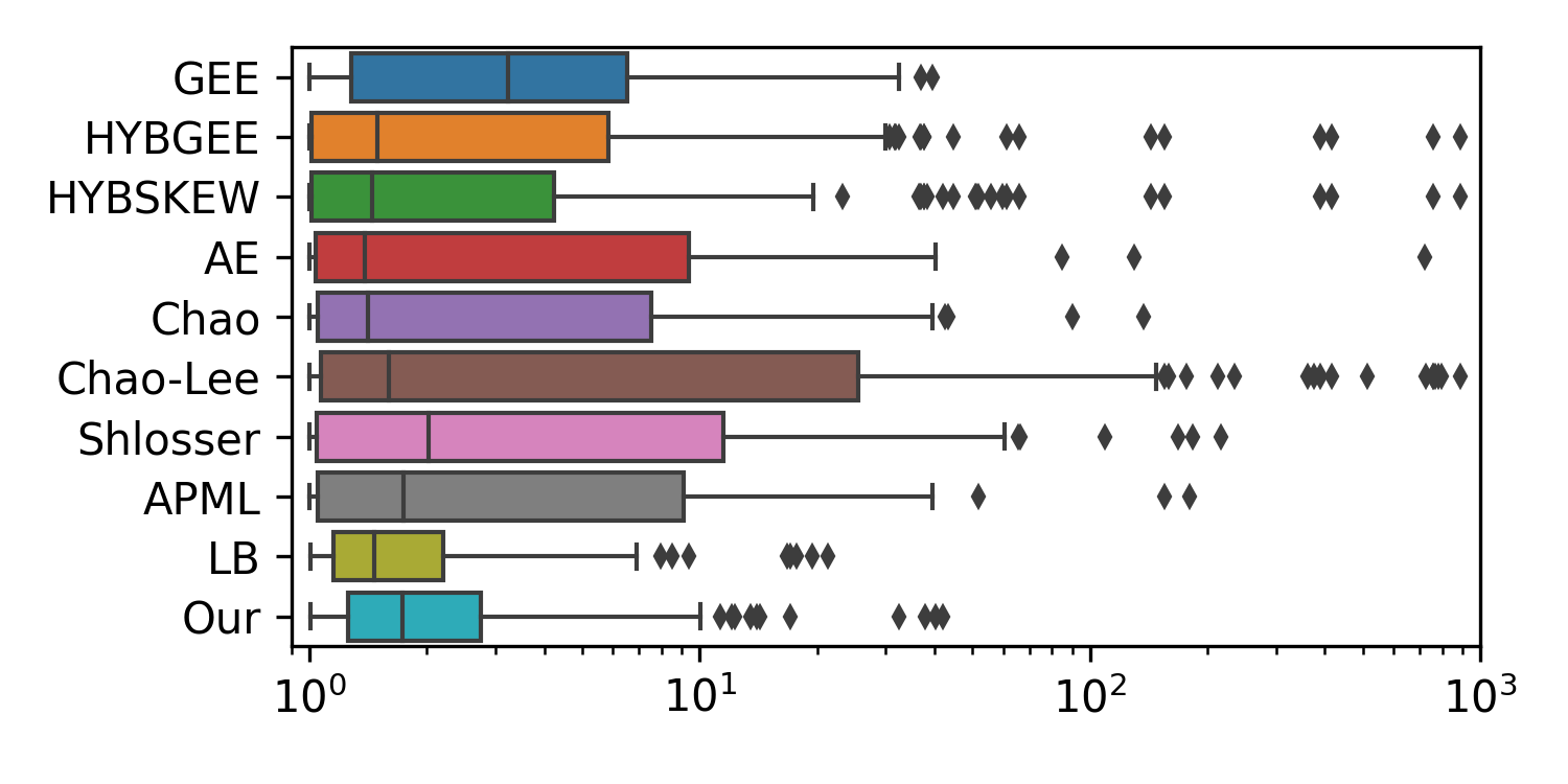
Ratio error distribution. To show the distribution and the worst case of ratio error, we plot the boxplot (box 2020) of ratio error in Figure 6 when sampling rate . Overall, our method has the smallest error in most cases and also has the smallest worst case error. In of cases, the ratio error of our method is smaller than , much better than all baselines. The worst case ratio error of our method is almost the same as the baseline GEE that has theoretical worst case ratio error guarantee. In of cases, the two hybrid methods HYBGEE and HYBSKEW are on average better than GEE but they are not stable and their worst case error can be as large as causing their averaged ratio error to be greater than GEE in Table 2.
6.3. Ablation Study
We perform ablation study to show the contribution of each component in our method and compare them to existing or straightforward solutions. Table 3 shows the results. Column "Full" denotes our method with full set of components. We ablate our method in three aspects, training data generation, model architecture and objective function for training. The symbol "-" denotes dropping the component that it precedes.
Training data generation. As shown in column "-diversify" in Table 3, when removing the diversify component proposed in Section 4.1.3, ratio error increases a bit, though the error is still significantly lower than the best performing baseline in Table 2. This verifies our intuition in Section 4.1.3: increasing the support region of the profiles is helpful to the generalization ability of our model. We also compare to four heuristic method of generating training data. "uni" denotes generating each of the population profile by a uniform distribution. "pl" denotes generating so that the relationship between and is power law. "rw" denotes generating by random walk, i.e. where is a random step size. "mix" denotes mixing all training data generated by the three heuristic methods. For the three heuristic methods, we also ensure that we introduce enough randomness by using a set of different random hyperparameters (e.g. length of , range of uniform distribution, parameters in power law distribution, and step size in random walk) for each data point. The results in Table 3 show that our way of generating training data outperforms the heuristic methods significantly. When mixing the three types of heuristically generated data together, the averaged error is smaller than using each type along because mixing all data increases training data diversity and helps the model to generalize better.
Model architecture. We drop the logarithm layer in our model architecture (Figure 3). As shown in column "-log" in Table 3, the ratio error increases dramatically. This validates our choice to take logarithm and its advantages as discussed in Section 4.2.2.
Training objective. Column "-b" in Table 3 denotes removing our proposed regularization for a worst-case optimal estimator in (19). Overall, contrasting the column "Full" to the column "-b", we can see adding the proposed regularization makes the overall ratio error decrease by , closing the gap to the empirical lower-bound by . This regularization pushes the model to a worst-case optimal estimator, and make it more robust (for datasets where it is not the best, it is close to the best-performing estimator). With this regularization, the ratio error on the most difficult datasets (e.g., Product, and Inventory) decreases significantly more than on other datasets. Removing this regularization does not make the learned estimator "optimal" in specific datasets, but the error may decrease a bit on the easy datasets (e.g., Kasandr, Airline, and DMV). We further drop the L2 regularization (column "-b-L2") and error further increases. This is expected as L2 regularization encourages sparse and small model parameters that generalize better. Finally, we further drop the logarithm on NDV (column "-b-L2-log") to use a naive mean squared loss on NDV and the error increases to be extremely high (similar to the "-log" column under "Model arch").
| Datasets | Full | Training data generation | Model arch | Training objective | ||||||
| -diver sify | heuristic | -log | -b | -b -L2 | -b-L2 -log | |||||
| uni | rw | pl | mix | |||||||
| Kasandr | 2.4 | 5.2 | 40.8 | 30.8 | >1k | 50.1 | >1k | 2.3 | 3.3 | >1k |
| Airline | 1.9 | 2.5 | 3.4 | 4.7 | 464.0 | 24.9 | >1k | 1.8 | 1.9 | >1k |
| DMV | 2.7 | 3.4 | 129.8 | 45.2 | 14.6 | 98.3 | >1k | 2.5 | 3.8 | >1k |
| Campaign | 3.9 | 6.7 | 147.9 | 176.5 | 933.1 | 127.9 | >1k | 3.9 | 21.6 | >1k |
| SSB | 2.0 | 3.3 | 19.1 | 1.2 | 6.5 | 3.1 | >1k | 2.1 | 1.8 | >1k |
| NCVR | 6.4 | 8.1 | 83.2 | 92.9 | >1k | 113.8 | >1k | 7.2 | 8.2 | >1k |
| Product | 14.6 | 20.1 | 417.6 | 227.3 | 52.7 | 658.5 | >1k | 20.4 | 22.0 | >1k |
| Inventory | 7.8 | 10.1 | 386.7 | 313.4 | >1k | 109.5 | >1k | 9.4 | 12.0 | >1k |
| Logistics | 3.5 | 9.2 | 496.7 | 390.6 | >1k | 115.5 | >1k | 3.8 | 4.8 | >1k |
| Average | 5.0 | 7.7 | 191.2 | 142.5 | >1k | 76.9 | >1k | 5.9 | 8.8 | >1k |

6.4. Sensitivity Analysis
We show the robustness of our method to the hyperparameters. Sensitivity to number of features. Our number of features is where is the number of elements in sample profile that used as raw features. We set by default. To test the sensitivity, we vary from 10 to 200. As shown in Figure 7(1), as increases from 100 to 200 ( increases from 106 to 206), averaged ratio error doesn’t change, so setting suffices.
Sensitivity to number of layers in network. The number of layers in our network is where . We vary from to so the number of layers varys from to . In addtion, we evaluate one extreme case and , where the network only has one linear layers with input dimenions and one output demension. The averaged ratio error with respect to the number of layers is shown in Figure 7(2). As the number of layer increases, averaged ratio error decreases due to the increase of model complexity. Although gives marginally better result, our choice with and gives good enough result.
Sensitivity to L2 regularization. Figure 7(3) shows the average ratio error under different L2 regularization parameter . The error is overall quite stable when is in region []. Error increases significantly when increases from to 1 and increases even more dramatically when increases from 1 to 10. This increasing trend in region is similar to the increasing trend of the training loss in Figure 4. Our heuristic method of selecting based on the training loss curve at the end of Section 4.3 is able to select . Although the optimal is at , is good enough.
Sensitivity to probability . Probability is the confidence level of our derived lower bound in (18). Figure 7(4) shows the averaged ratio error when probability varies in region . Overall, the averaged ratio error is quite stable. The optimal value for is about . We heuristically selected to be in Section 4.3. Although it is not the optimal, is good enough.
Sensitivity to number of training data points. We vary the number of training data points from to . In Figure 8, the averaged ratio error decreases significantly as increases because more training data improves the generalization ability of the model. However, as further increases, averaged ratio error increases marginally and then stabilizes. This counter-intuitive phenomenon happens often when the distribution of training set is different from the test set. When the training set becomes extremely large, the model learns the very fine-grained details of the training distribution, which tend to not generalize better to the test set.
Choosing training data size. Note that the best choice of training data sizes for different columns can be different. Our goal is to train a workload-agnostic estimator, and it can be too expensive (if not impossible) to tune the training data size for each different workload. From Figure 8, which reports the average error across a number of tables for varying , a general trend is that: after exceeds some threshold (e.g., ), the performance of the learned estimator stabilizes. Thus, in practice, we simply choose a training data size that is large enough (exceeding the threshold) but does not make the training data preparation and model training too expensive. We set the training data size to train the estimator (available in (Library 2021)) used in all the other experiments.

Out-of-range generalization. In our training set, the max population size is and the max population NDV is . To evaluate the out-of-range performance, i.e., estimation for a column with large NDV not seen at training time, of our learned estimator, we create such extended test datasets: for each column in the original test datasets, we duplicate it times and add a suffix to each value in the th duplicate. In this way, columns in the extended datasets have extremely large population sizes (maximum at ) and NDVs (maximum at ). We focus on columns with population size in and population NDV in , and report the average ratio error for all methods with sampling rate on these columns in Table 4. Note that both the original and extended test datasets are not used for training our estimator. It can be seen that our method also works very well even when NDV to be estimated is out-of-range, and is still better than other baselines. The out-of-range generalizability of our learned estimator is partly due to the logarithm operations as discussed in Section 4.2.2.
| GEE | HYB GEE | HYB SKEW | AE | Chao | Chao -Lee | Shlo sser | APML | Our | |
| Avg ratio error | 20.6 | 30.1 | 78.3 | 15.6 | 143.2 | 164.5 | 15.7 | 37.5 | 4.2 |
7. Conclusion and Future work
In this paper, we consider a fundamental question: whether it is possible to train a workload-agnostic machine learning model to approximate principled statistical estimators such as maximum likelihood estimators (MLE). We provide a positive answer to this question on the concrete task of estimating the number of distinct values (NDV) of a population from a small sample. We formulate the sample-based NDV estimation problem as an MLE problem which, however, is difficult to be solved even approximately. We propose a learning-to-estimate framework to train a workload-agnostic model to approximate the MLE estimator. Extensive experiments on nine datasets from diverse domains demonstrate that our learned estimator is robust and outperforms all baselines significantly.
For future work, we would like to extend our learning-to-estimate method to learn estimators for other properties whose MLE is difficult to obtain, e.g., entropy and distance to uniformity.
8. Appendix
8.1. From sample to sample profile
We first formally show that the NDV that maximizes the likelihood of observing the sample is identical to the NDV that maximizes the likelihood of observing the sample profile . Consider two samples and with the same sample profile , there must exist a “relabeling” of values, i.e., a permutation where is the domain of all possible values, such that . For every possible column of , we can apply the same relabeling to . Since relabeling doesn’t change the probability of generating the sample, we have
| (21) |
For estimators to be applied to any unseen columns with arbitrary values, it is natural to regard that the specific values provide no information on NDV. In other words, relabeling does not change the probability of a column when conditioned on NDV: . Therefore,
| (22) |
This means:
| (23) |
where denotes the set of samples whose profile is . Therefore:
| (24) |
This means using sample profile is theoretically identical to using sample. However, using profile is practically advantageous than using sample because profile is a more compact representation and the input dimensionality is reduced. This makes the likelihood function much simpler. In addition, we are to train a model as an estimator and smaller input feature dimensionality makes learning easier.
8.2. Proof of Proposition 1
Proposition 1.
For any size- sample with profile and NDV , there exist two size- columns and with NDVs and , respectively, such that with probability at least we cannot distinguish whether the observed is generated from or from , with
| (25) |
for and .
Proof.
Consider two columns (multi-sets) and sharing the common subset . Suppose is a multi-set with size and NDV . Let be a multi-set containing values that are not in , each appearing exactly once in , and be a size- multi-set containing only values that already have appeared in . Thus, the two multi-sets and have NDVs and , respectively.
We draw a size- sample from uniformly at random without replacement11 1 Analysis for the case with replacement is similar and simpler, and is omitted here.. When drawing the th value ,
and thus, the probability that contain values only from is
| (26) | ||||
Similarly, for a size- sample drawn from uniformly at random, we have .
After a sample profile is observed, since conditioned on and , and (profiles of and , respectively) follow the same distribution, i.e., , we cannot distinguish whether the underlying data column is or . From (26), we have
where the last inequality follows from the claim that for , which can be easily verified.
Moreover, we want to ensure that and both cover all the distinct values of , i.e., sample NDVs and NDV of are all . Suppose each distinct value appears with the same frequency in . From the Coupon Collector’s problem (Section 3.6.2 in (Motwani and Raghavan 1995)), conditioned on , , and , with probability at least (for ), a size- sample (or ) contains each of the distinct values in at least once. Therefore, we have
Let and thus .
For (which ensures , i.e., a sufficient number of values can be drawn from into or ) and (from our choice of and ), we can conclude that, with probability at least , we cannot distinguish whether is from or from , with desired NDVs and in (25).
8.3. Proof of Theorem 1
Theorem 1.
For any size- sample with profile and sample NDV observed (where ), with probability , there exist a choice of column with NDV such that any estimation of based on , i.e., , has ratio error at least
| (27) |
Proof.
Consider the two choices of columns and constructed in Proposition 1, with NDVs and , respectively, as in (25). Since with probability at least , we cannot distinguish whether is from or , for , the ratio error is at least , which is minimized when . And thus, the lower bound of ratio error in (27) follows for the choice of and in (25).
References
- (1)
- air (2020) 2020. Airlines Departure Delay. https://www.openml.org/d/42728
- box (2020) 2020. Box plot. https://en.wikipedia.org/wiki/Box_plot
- bts (2020) 2020. Bureau of Transportation Statistics. https://www.transtats.bts.gov/
- Cam (2020) 2020. Campaign finance data. https://www.fec.gov/data/
- dat (2020) 2020. Department of Motor Vehicle (DMV) Office Locations. https://catalog.data.gov/dataset/department-of-motor-vehicle-dmv-office-locations
- lea (2020) 2020. Leaky ReLU. https://pytorch.org/docs/stable/generated/torch.nn.LeakyReLU.html
- max (2020) 2020. MaxCompute. https://www.alibabacloud.com/product/maxcompute
- pyd (2020) 2020. Pydistinct - Population Distinct Value Estimators. https://pydistinct.readthedocs.io/
- ran (2020) 2020. Random numbers that add to 100: Matlab. https://stackoverflow.com/questions/8064629/random-numbers-that-add-to-100-matlab
- bre (2020) 2020. scipy.optimize.brentq. https://docs.scipy.org/doc/scipy/reference/generated/scipy.optimize.brentq.html
- sko (2020) 2020. skorch documentation. https://skorch.readthedocs.io/en/stable/
- nvc (2020) 2020. Voter Registration Statistics. https://www.ncsbe.gov/results-data/voter-registration-data
- met (2020) 2020. weight decay in neural networks. https://metacademy.org/graphs/concepts/weight_decay_neural_networks
- rfs (2021) 2021. Random Vectors with Fixed Sum - File Exchange - MATLAB Central. https://www.mathworks.com/matlabcentral/fileexchange/9700-random-vectors-with-fixed-sum [Online; accessed 27. Apr. 2021].
- Anagnostopoulos and Triantafillou (2015) Christos Anagnostopoulos and Peter Triantafillou. 2015. Learning to accurately count with query-driven predictive analytics. In 2015 IEEE international conference on big data (big data). IEEE, 14–23.
- Bishop (2006) Christopher M Bishop. 2006. Pattern recognition and machine learning. springer.
- Brent (1973) Richard P Brent. 1973. Algorithms for Minimization without Derivatives, chap. 4.
- Bunge and Fitzpatrick (1993) John Bunge and Michael Fitzpatrick. 1993. Estimating the number of species: a review. J. Amer. Statist. Assoc. 88, 421 (1993), 364–373.
- Chambers et al. (2012) Raymond L Chambers, David G Steel, Suojin Wang, and Alan Welsh. 2012. Maximum likelihood estimation for sample surveys. CRC Press.
- Chao (1984) Anne Chao. 1984. Nonparametric estimation of the number of classes in a population. Scandinavian Journal of statistics (1984), 265–270.
- Chao and Lee (1992) Anne Chao and Shen-Ming Lee. 1992. Estimating the number of classes via sample coverage. Journal of the American statistical Association 87, 417 (1992), 210–217.
- Charikar et al. (2000) Moses Charikar, Surajit Chaudhuri, Rajeev Motwani, and Vivek Narasayya. 2000. Towards estimation error guarantees for distinct values. In Proceedings of the nineteenth ACM SIGMOD-SIGACT-SIGART symposium on Principles of database systems. 268–279.
- Charikar et al. (2019) Moses Charikar, Kirankumar Shiragur, and Aaron Sidford. 2019. Efficient profile maximum likelihood for universal symmetric property estimation. In Proceedings of the 51st Annual ACM SIGACT Symposium on Theory of Computing. 780–791.
- Chaudhuri et al. (2017) Surajit Chaudhuri, Bolin Ding, and Srikanth Kandula. 2017. Approximate Query Processing: No Silver Bullet. In SIGMOD. 511–519.
- Cohen and Nezri (2019) Reuven Cohen and Yuval Nezri. 2019. Cardinality Estimation in a Virtualized Network Device Using Online Machine Learning. IEEE/ACM Transactions on Networking 27, 5 (2019), 2098–2110.
- Dutt et al. (2020) Anshuman Dutt, Chi Wang, Vivek R. Narasayya, and Surajit Chaudhuri. 2020. Efficiently Approximating Selectivity Functions using Low Overhead Regression Models. Proc. VLDB Endow. 13, 11 (2020), 2215–2228.
- Dutt et al. (2019) Anshuman Dutt, Chi Wang, Azade Nazi, Srikanth Kandula, Vivek Narasayya, and Surajit Chaudhuri. 2019. Selectivity estimation for range predicates using lightweight models. Proc. VLDB Endow. 12, 9 (2019), 1044–1057.
- Flajolet et al. (2007) Philippe Flajolet, Éric Fusy, Olivier Gandouet, and Frédéric Meunier. 2007. Hyperloglog: the analysis of a near-optimal cardinality estimation algorithm. In Proceedings of the Analysis of Algorithms Conference. 137–156.
- Goodfellow et al. (2017) Ian Goodfellow, Yoshua Bengio, and Aaron Courville. 2017. Deep learning Ch. 5 Machine Learning Basics. The MIT Press, 132–133.
- Haas et al. (1995) Peter J Haas, Jeffrey F Naughton, S Seshadri, and Lynne Stokes. 1995. Sampling-based estimation of the number of distinct values of an attribute. In VLDB, Vol. 95. 311–322.
- Haas and Stokes (1998) Peter J Haas and Lynne Stokes. 1998. Estimating the number of classes in a finite population. J. Amer. Statist. Assoc. 93, 444 (1998), 1475–1487.
- Hao and Orlitsky (2019) Yi Hao and Alon Orlitsky. 2019. The broad optimality of profile maximum likelihood. In Advances in Neural Information Processing Systems. 10991–11003.
- Harmouch and Naumann (2017) Hazar Harmouch and Felix Naumann. 2017. Cardinality estimation: An experimental survey. Proceedings of the VLDB Endowment 11, 4 (2017), 499–512.
- Haykin (1998) Simon Haykin. 1998. Neural Networks: A Comprehensive Foundation. Prentice Hall.
- Hilprecht et al. (2020) Benjamin Hilprecht, Andreas Schmidt, Moritz Kulessa, Alejandro Molina, Kristian Kersting, and Carsten Binnig. 2020. DeepDB: learn from data, not from queries! Proceedings of the VLDB Endowment 13, 7 (2020), 992–1005.
- Hines (1996) J Wesley Hines. 1996. A logarithmic neural network architecture for unbounded non-linear function approximation. In Proceedings of International Conference on Neural Networks (ICNN’96), Vol. 2. IEEE, 1245–1250.
- Ioffe and Szegedy (2015) Sergey Ioffe and Christian Szegedy. 2015. Batch Normalization: Accelerating Deep Network Training by Reducing Internal Covariate Shift. In Proceedings of the 32nd International Conference on International Conference on Machine Learning - Volume 37 (Lille, France) (ICML’15). JMLR.org, 448–456.
- Juszczak et al. ([n.d.]) Piotr Juszczak, D Tax, and Robert PW Duin. [n.d.]. Feature scaling in support vector data description. Citeseer.
- Kiefer et al. (2017) Martin Kiefer, Max Heimel, Sebastian Breß, and Volker Markl. 2017. Estimating join selectivities using bandwidth-optimized kernel density models. Proceedings of the VLDB Endowment 10, 13 (2017), 2085–2096.
- Kingma and Ba (2015) Diederik P. Kingma and Jimmy Ba. 2015. Adam: A Method for Stochastic Optimization. In 3rd International Conference on Learning Representations, ICLR 2015, San Diego, CA, USA, May 7-9, 2015, Conference Track Proceedings, Yoshua Bengio and Yann LeCun (Eds.). http://arxiv.org/abs/1412.6980
- Kipf et al. (2018) Andreas Kipf, Thomas Kipf, Bernhard Radke, Viktor Leis, Peter Boncz, and Alfons Kemper. 2018. Learned cardinalities: Estimating correlated joins with deep learning. arXiv preprint arXiv:1809.00677 (2018).
- Lakshmi and Zhou (1998) Seetha Lakshmi and Shaoyu Zhou. 1998. Selectivity estimation in extensible databases-a neural network approach. In VLDB, Vol. 98. 24–27.
- Library (2021) Library. 2021. An learned sample-based NDV estimator. https://github.com/wurenzhi/learned_ndv_estimator. [Online; accessed 11-October-2021].
- Liu et al. (2015) Henry Liu, Mingbin Xu, Ziting Yu, Vincent Corvinelli, and Calisto Zuzarte. 2015. Cardinality estimation using neural networks. In Proceedings of the 25th Annual International Conference on Computer Science and Software Engineering. 53–59.
- Metwally et al. (2008) Ahmed Metwally, Divyakant Agrawal, and Amr El Abbadi. 2008. Why go logarithmic if we can go linear? Towards effective distinct counting of search traffic. In Proceedings of the 11th international conference on Extending database technology: Advances in database technology. 618–629.
- Mohamadi et al. (2017) Hamid Mohamadi, Hamza Khan, and Inanc Birol. 2017. ntCard: a streaming algorithm for cardinality estimation in genomics data. Bioinformatics 33, 9 (2017), 1324–1330.
- Motwani and Raghavan (1995) Rajeev Motwani and Prabhakar Raghavan. 1995. Randomized Algorithms. Cambridge University Press.
- Motwani and Vassilvitskii (2006) Rajeev Motwani and Sergei Vassilvitskii. 2006. Distinct values estimators for power law distributions. In 2006 Proceedings of the Third Workshop on Analytic Algorithmics and Combinatorics (ANALCO). SIAM, 230–237.
- Nath et al. (2008) Suman Nath, Phillip B Gibbons, Srinivasan Seshan, and Zachary Anderson. 2008. Synopsis diffusion for robust aggregation in sensor networks. ACM Transactions on Sensor Networks (TOSN) 4, 2 (2008), 1–40.
- O’Neil et al. (2007) Patrick E O’Neil, Elizabeth J O’Neil, and Xuedong Chen. 2007. The star schema benchmark (SSB).
- Pavlichin et al. (2019) Dmitri S Pavlichin, Jiantao Jiao, and Tsachy Weissman. 2019. Approximate Profile Maximum Likelihood. Journal of Machine Learning Research 20, 122 (2019), 1–55. http://jmlr.org/papers/v20/18-075.html
- Raghu et al. (2017) Maithra Raghu, Ben Poole, Jon M. Kleinberg, Surya Ganguli, and Jascha Sohl-Dickstein. 2017. On the Expressive Power of Deep Neural Networks. In Proceedings of the 34th International Conference on Machine Learning, ICML 2017. 2847–2854.
- Shlosser (1981) A Shlosser. 1981. On estimation of the size of the dictionary of a long text on the basis of a sample. Engineering Cybernetics 19, 1 (1981), 97–102.
- Shorten and Khoshgoftaar (2019) Connor Shorten and Taghi M Khoshgoftaar. 2019. A survey on image data augmentation for deep learning. Journal of Big Data 6, 1 (2019), 60.
- Sidana et al. (2017) Sumit Sidana, Charlotte Laclau, Massih R Amini, Gilles Vandelle, and André Bois-Crettez. 2017. KASANDR: a large-scale dataset with implicit feedback for recommendation. In Proceedings of the 40th International ACM SIGIR Conference on Research and Development in Information Retrieval. 1245–1248.
- Ting (2019) Daniel Ting. 2019. Approximate Distinct Counts for Billions of Datasets. In Proceedings of the 2019 International Conference on Management of Data (Amsterdam, Netherlands) (SIGMOD ’19). Association for Computing Machinery, New York, NY, USA, 69–86. https://doi.org/10.1145/3299869.3319897
- Van Laarhoven (2017) Twan Van Laarhoven. 2017. L2 regularization versus batch and weight normalization. arXiv preprint arXiv:1706.05350 (2017).
- Wang et al. (2021) Xiaoying Wang, Changbo Qu, Weiyuan Wu, Jiannan Wang, and Qingqing Zhou. 2021. Are We Ready for Learned Cardinality Estimation? Proc. VLDB Endow. 14, 9 (May 2021), 1640–1654. https://doi.org/10.14778/3461535.3461552
- Xu et al. (2021) Keyulu Xu, Mozhi Zhang, Jingling Li, Simon S Du, Ken-ichi Kawarabayashi, and Stefanie Jegelka. 2021. How neural networks extrapolate: From feedforward to graph neural networks. In ICLR.
- Zhu et al. (2021) Rong Zhu, Ziniu Wu, Yuxing Han, Kai Zeng, Andreas Pfadler, Zhengping Qian, Jingren Zhou, and Bin Cui. 2021. FLAT: Fast, Lightweight and Accurate Method for Cardinality Estimation. Proc. VLDB Endow. 14, 9 (May 2021), 1489–1502. https://doi.org/10.14778/3461535.3461539