Enhancing variational generation through self-decomposition
Abstract
In this article we introduce the notion of Split Variational Autoencoder (SVAE), whose output is obtained as a weighted sum of two generated images , and is a learned compositional map. The composing images , as well as the -map are automatically synthesized by the model. The network is trained as a usual Variational Autoencoder with a negative loglikelihood loss between training and reconstructed images. No additional loss is required for or , neither any form of human tuning. The decomposition is nondeterministic, but follows two main schemes, that we may roughly categorize as either “syntactic” or “semantic”. In the first case, the map tends to exploit the strong correlation between adjacent pixels, splitting the image in two complementary high frequency sub-images. In the second case, the map typically focuses on the contours of objects, splitting the image in interesting variations of its content, with more marked and distinctive features. In this case, according to empirical observations, the Fréchet Inception Distance (FID) of and is usually lower (hence better) than that of , that clearly suffers from being the average of the former. In a sense, a SVAE forces the Variational Autoencoder to make choices, in contrast with its intrinsic tendency to average between alternatives with the aim to minimize the reconstruction loss towards a specific sample. According to the FID metric, our technique, tested on typical datasets such as Mnist, Cifar10 and CelebA, allows us to outperform all previous purely variational architectures (not relying on normalization flows).
Index Terms:
Deep learning, Generative modeling, Multi-layer Neural Networks, Representation learning, Unsupervised learning, Variational AutoEncoder.I Introduction
Generative modeling (see e.g. [27] for an introduction) is one of the most fascinating problems in Artificial Intelligence, with many relevant applications in different areas comprising computer vision, natural language processing, medicine or reinforcement learning. The goal is not only to be able to sample new realistic examples starting from a given set of data, but to gain insight in the data manifold, and the way a neural network is able to extract and exploit the characteristic features of data. In case of high-dimensional data, the generative problem can only be addressed by means of Deep Neural Networks, and this topic led to tremendous research in many different directions, particularly nourishing the recent field of unsupervised representation learning.
Among the different kind of generative models which have been investigated, Variational Autoencoders (VAEs) [18, 26] have always exerted a particular fascination [35, 34, 29], mostly due to their strong theoretical foundations, that will be briefly recalled in Section II. Unfortunately, results remained below expectations, and the generative quality of VAEs is systematically outperformed by different generative techniques like e.g. Generative Adversarial Networks.
A particularly annoying problem is that VAEs produce images with a characteristic blurriness, very hard to be removed with traditional techniques [28, 20]. The source of the problem is not easy to identify, but it is likely due to averaging, implicitly underlying the VAE frameworks and, more generally, any autoencoder approach. As observed in [11]. In presence of multimodal output, a loglikelihood objective typically results in averaging and hence blurriness. A GAN does not have this problem, since its goal is to fool the Discriminator, not to reconstruct a given input. Since Variational Autoencoders are intrinsically multimodal, both due to dimensionality reduction, and to the sampling process during training, a certain amount of blurriness is unfortunately expected.


Starting from the averaging assumption [2], it is natural to try to address blurriness by offering to the Variational Autoencoder the possibility to create multiple images, and then synthesize a result as a (learned) weighted combination of them. This is precisely what our Split Variational Autoencoder (SVAE) is supposed to do: the generator returns two images and a probability map with the same spatial dimension of the images, and synthesize a resulting image where is point-wise multiplication (broadcasted over channels). The Autoencoder is trained by minimizing the reconstruction loss between and , together with the traditional regularization component over latent variables. No additional loss is imposed over , or .
The resulting decomposition is non deterministic, mostly depending on the network architecture and the dimension of the latent space. However, it seems to follow two main schemes, that we call “syntactic” (see Figures 1, 3), and “semantic” (see Figures 2, 4). In this Figures, the top line is the map, the second line is , the third line is , and in the last line we have . Let us also remark that all images in the pictures have been generated, not reconstructed.


In the first case, the map takes advantage of the strong correlation between adjacent pixels splitting the image in two complementary high frequency sub-images. Each image has more freedom in filling the ignored parts, easing the generative task.
In the second, even more interesting case, the map focuses on the contours of objects, splitting the image in interesting variations around them, typically resulting in more marked and distinctive features. In this case, the Fréchet Inception Distance (FID) of and may also be lower (hence better) than that of , that apparently suffers from being the average of the former.
An interesting aspect of SVAEs, and possibly one of reasons behind their effectiveness, is that they allow to work with a number of latent variables sensibly higher than usual, hence implicitly addressing the variable collapse phenomenon [6, 36, 31, 25, 1]. This seems to be an indication that self-splitting is indeed a convenient way to induce the model to synthesize a large number of uncorrelated latent features.
We tested SVAE on typical datasets such as Mnist, Cifar10 and CelebA, and in all cases we observed substantial improvements w.r.t. the “vanilla” approach. Excluding models that make use of sophisticated techniques like normalizing flows [16, 32, 23] (typically requiring thousands of latent variables, and practically hindering a fruitful exploration of the latent space), SVAE outperforms all previous variational architectures.
The code relative to this work can be accessed on Github in the following public repository: https://github.com/asperti/Split-VAE Pretrained weights for the models discussed in the article are available at the following page: https://www.cs.unibo.it/~asperti/SVAE.html.
I-A Structure of the article
In Section II we briefly recall the theory behind Variational Autoencoder, show their encoder-decoder architecture (Section II-A), and discuss some aspects related to the dimension of the latent space and the so called variable-collapse phenomenon (Section II-B). Section III introduces the notion of Split Variational Autoencoder and provides a detailed description of the ResNet-like architecture used in our experiments. In Section IV we outline our experimental setting, discussing the metrics and datasets used for the benchmarks. Quantitative results are given in Section V along with a critical discussion. Ablation investigations are debated in Section VI. In the Conclusions VII, we summarize the content of the article and outline research directions for future developments.
II Background
There exist in the literature several good introductions to Variational Autoencoders (VAEs) [9, 19, 4], so in this section we provide a quite short introduction to the topic, mostly with the purpose to fix notation and terminology.
In a latent variable approach, the probability distribution of a data point is expressed through marginalization over a vector of latent variables:
| (1) |
where is the latent encoding of distributed with a known distribution named prior distribution. If we can learn a good approximation of from the data, we can use it to generate new samples via ancestral sampling:
- •
sample .
- •
generate .
Supposing to have a parametric family of probability distributions (e.g. modelled by a neural network), the goal is to find that optimize the loglikelihood over all (MLE):
| (2) |
Addressing directly the previous optimization problem is usually computationally infeasible. For this reason, VAEs exploit another probability distribution named inference (or encoder) distribution, expressing the relation between a data point and its associated latent representation . Hopefully, should approximate , so that their Kullback-Leibler divegence
should be small. Further expanding the previous equation, we get:
Hence,
| (3) |
Recalling that is always positive, we get
stating that the left hand side is a lower bound for the loglikelihood of , known as Evidence Lower Bound (ELBO).
Since ELBO is more tractable than MLE, it is used as the cost function for training of neural networks. Optimizing ELBO we are jointly improving the loglikelihood of , and implicitly minimizing the distance between and .
The ELBO has a form similar to an autoencoder: the inference distribution encodes the input to its latent representation , and decodes back to .
For generative sampling, we just exploit the decoder, sampling latent variables according to the prior distribution (that must be known).
II-A Vanilla VAE and its training
In the vanilla VAE, we assume to be a Gaussian (spherical) distribution , so that learning amounts to learning its two first moments. It is important to know the variance since during training we need to sample according to .
Similarly, we also assume to have Gaussian distribution centered around a decoder function . The functions , and are modelled by deep neural networks.
Supposing that the model approximating the decoder function is sufficiently expressive, the shape of the prior distribution does not really matter, and it is traditionally assumed to be a normal distribution .
Under these assumptions, the term is the KL-divergence between two Gaussian distributions and that has the following closed form expression:
| (4) |
where is the dimension of the latent space.
Coming to the reconstruction loss , under the Gaussian assumption, the logarithm of is proportional to the quadratic distance between and its reconstruction ; the variance of this Gaussian distribution can be understood as a parameter balancing the relative importance between reconstruction error and KL-divergence [9, 5].
The problem of integrating sampling with backpropagation during training is addressed by the so called reparametrization trick [18, 26]: sampling is performed using a standard distribution outside of the backpropagation flow and this value is rescaled with and .
It is important to stress that sampling at training time has no relation with ancestral sampling for generation (we do not have at generation time!). The purpose of sampling at training time is to provide estimates for the main moment of , that are then subject to KL-regularization. In turn, the final goal of this regularization is to bring the marginal inference distribution close to the prior .
II-B The dimension of the latent space
A critical aspect of VAEs is the dimension of the latent space. Typically, having many latent variables reduces the compression loss and improves reconstruction. However, this may not result in an improvement of the generative model: more variables we have and the harder is to ensure their independence and force them to assume the desired prior distribution. We may try to tame them by strengthening the KL-regularization component in the loss function, in the spirit of a -VAE [13, 7], but this typically results in the collapse of the less informative variables, that get completely ignored by the decoder [6, 36, 31, 25, 1]. A collapsed variable has a very characteristic behaviour: since it is ignored by the decoder, it is free to minimize KL-regularization, with a mean value and a variance for any .
A more expressive architecture may typically result in a better exploitation of latent variables, allowing to work with a larger number of them. The dimension of the latent space also reflects the complexity of the data manifold: for instance, with non-hierarchical architectures, it is customary to work with 16 variables for Mnist, 128 variables for Cifar10 and 64 variables for CelebA. As we shall see, with a SVAE we can sensibly enlarge these numbers.
III Split-VAE
The general notion of VAE does not impose any specification on the architecture of the encoder and the decoder, and many different variants have been investigated in the literature: dense, convolutional, with residuality, with autoregressive flows, hierarchical, and so on (see e.g. [34, 4] for a discussion).
A Split-VAE (SVAE) is just another architectural variant: we do not touch the theory or the loss function. In a SVAE the output is computed as a weighted sum
of two generated images , and is a learned compositional map. Typically, to turn a vanilla VAE into a Split-VAE it is enough to change the number of channels of the last layer of the network: in case of a grayscale image, passing from 1 to 3, and in case of a color image passing from 3 to 1+3+3=7 (the map and two color images ). The compound image can be computed internally of externally to the network, as part of the loss function. Since the increased number of channels only concerns the very last layer, the total number of parameters remains comparable to the vanilla version.
The philosophy underlying a SVAE has been already discussed in the introduction: we merely create an opportunity to be exploited by the model. From a more practical perspective, it can be be understood as a way to induce diversification in the features learned by the network, via a simple but highly effective self-attention mechanism [33]. From this point of view, it is not too far from techniques like squeeze and excitation [14] or feature-wise linear modulation [24]; the main difference is that we operate on the visible level, and along spatial dimensions. This allows us, among other things, to provide intelligible visualizations of the splitting learned by the network.
One of main characteristic of Split-VAEs is that they allow to work with a sensibly larger number of latent variables: 32 for Mnist, 200 for Cifar10 and 150 for CelebA. This testifies the diversification of latent features, and partially explains the improved generative quality.
III-A Encoder-decoder architecture
For the implementation of the encoder and the decoder we adopted a ResNet-like architecture derived from [8] that we already used in previous works [5, 4]; this allows us to do a fair comparison of the split-technique with previous approaches, without additional biases. The network architecture is schematically described in Figure 6.
| (a) | ||||
|

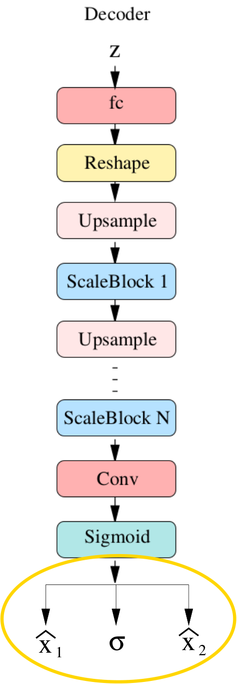
The encoder is a fully convolutional model where the input is progressively downsampled for a configurable number of times, jointly doubling the number of channels. Before downsampling, the input is processed by a so called Scale Block, that is just a sequence of Residual Blocks. A Residual Block is an alternated sequence of BatchNormalization and spatial preserving Convolutional layers, intertwined with residual connections. The number of Scale Blocks at each scale of the image pyramid, the number of Residual Blocks inside each Scale Block, and the number of convolutions inside each Residual Block are user configurable hyperparameters.
In the encoder, after the last Scale Block, a global average level extracts spatial agnostic features. These are first passed through a so called Dense Block (similar to a Residual Block but with dense layers instead of convolutions), and finally used to synthesize mean and variance for latent variables. The decoder first maps the internal encoding to a small map of dimension via a dense layer suitably reshaped. This is then up-sampled to the final expected dimension, inserting a configurable number of Scale Blocks at each scale.
IV Experimental setting
We compare the performance of SVAE with state-of-the-art variational autoencoders comprising Two-stage models [8, 5, 4], and Regularized Autoencoders [10]. We are not considering models relying on normalizing flows, such as [16, 32, 23]: these models typically require thousands of latent variables making them of relatively little interest from the point of view of representation learning.
For the comparison, we used traditional datasets, such as MNIST, CIFAR-10 [21] and CelebA [22]; the metrics adopted is the usual Frechèt Inception Distance [12] (FID), shortly discussed in section IV-A. All comparative results reported Section V are borrowed from the original publications.
In addition to the FID-score for generated images (GEN field, in Tables), we also provide an ex-post estimation of the probability distribution of the latent-space. This is done through a second VAE in [8, 5], and by fitting a Gaussian Mixture Model (GMM) in [10] (a normalizing autoregressive flow can be used with a similar purpose [17, 23]). Although possibly less expressive, the GMM technique is simple and effective, so we use it in our experiments (this aspect is somewhat orthogonal to the content of this article). The FID-score after resampling in the latent space is reported in the GMM entry, in the following Tables.
For each architecture, we also provide the number of parameters as an indicative measure of its complexity and energetic footprint (according to recent investigations [3], the number of parameters seem to provide a more reliable measure of efficiency than the number of Floating Point Operations).
IV-A Frechèt Inception Distance
The Frechèt Inception Distance [12] (FID) does not try to assess the “quality” of a single generated sample but merely compares the overall probability distribution of generated vs. real images. The dimension of the visible space is typically too large to allow a direct comparison; the main idea behind FID is to use, instead of raw data, their internal representations generated by some third party, agnostic network. In the case of FID, the Inception v3 network [30] trained on Imagenet is used to this purpose. The activations that are traditionally used are those relative to the last pooling layer, resulting in a vector of 2048 features.
Let and be the activations relative to real and generated images, and , their empirical mean and covariance matrix, respectively. Then the Frèchet Distance between and is the just the squared Wasserstein distance, namely:
| (5) |
where is the trace of the matrix.
V Numerical Results
In this section we give numerical results relative to Mnist, CIFAR-10 and CelebA, discussing the training process and the relevant hyperparameters.
V-A Mnist
In the case of Mnist we worked with a latent space of dimension 32, in contrast with the traditional dimension of 16. We tested several versions, with different balancing -factor between reconstruction and KL-regularization: we report results for and . Even when starting with the relatively high balancing factor , the number of inactive variables at the end of training is low: between 2 and 5. In all our experiments, the -factor is progressively reduced along training in order to preserve the initial balance between the two components, as described in [5].
In the case of Mnist, both syntactic and semantic decomposition (see Figures 1 and 2) usually give good results on the compound image, slightly better in the latter case.
Training lasted 300 epochs, using Adam optimizer with a learning rate of . Numerical results in terms of FID-scores are given in TableI.
| model | params | GEN | GMM |
|---|---|---|---|
| RAE-GP [10] | 22,386,449 | ||
| RAE-L2 [10] | 22,386,449 | ||
| RAE-SN [10] | 22,386,449 | ||
| 2S-VAE, [8] | 9,032,769 | ||
| 2S-VAE, [5] | 9,032,769 | ||
| SVAE () | 12,793,667 | ||
| SVAE () | 12,793,667 |
In [10], they observed that enlarging the number of components beyond 10 was not beneficial. However, in our case, presumably due to the larger number of latent variables, we found convenient to use a larger mix. In TableI we compare the cases of and components. To have an acceptable generative score before GMM-resampling we need to work with a high factor, like e.g. ; however, resampling compensates the need of regularization, and we obtain the best results with and 100 components.
See Figure 7 for examples of generated Mnist-like digits.


V-B Cifar10
CIFAR-10 confirms its somehow pathological nature. The complexity of the dataset can be readily appreciated by looking at the pictures in Figure 9 where we compare the mean images for CIFAR-10 and CelebA: the former is completely gray, while the latter is a relatively well defined “average” face (also observe, by the way, the strong bias of the CelebA dataset towards feminine, frontal, young, smiling faces).
 |
 |
| mean CIFAR-10 | mean CelebA |
Another interesting indicator of the complexity of CIFAR-10 is given by the FID score between each category and the full dataset (we derive 10000 image per category by flipping images in the training set, and compare them with the test-set). The score is extremely high, in spite of the fact that the “texture” is apparently quite similar. The FID score “magically” drops to 5.3 for a random mix.
| label | fid | label | fid | label | fid | label | fid |
|---|---|---|---|---|---|---|---|
| plane | 80.7 | car | 98.3 | bird | 65.0 | cat | 60.8 |
| deer | 66.3 | dog | 74.3 6 | frog | 100.2 | horse | 84.3 |
| ship | 97.7 | truck | 107.5 | mix | 5.3 | ||
Coming to SVAE, in the case of CIFAR-10, splitting produces results of the kind described in Figure 8. The FID scores for and are usually lower to that of testifying that the network is attempting a “semantic” decomposition; however, our networks failed, apart exceptions, to generate recognizable contours. In spite of this problem, numerical results, reported in Table III are quite good.
| model | params | GEN | GMM |
|---|---|---|---|
| RAE-GP [10] | 30,510,339 | ||
| RAE-L2 [10] | 30,510,339 | ||
| RAE-SN [10] | 30,510,339 | ||
| 2S-VAE [8] | 27,766,275 | ||
| 2S-VAE, [5] | 27,766,275 | ||
| SVAE | 13,061,143 |
These results have been obtained exploiting a latent space of dimension 200 (in contrast with the traditional dimension of 128) and a balancing factor between reconstruction and KL-regularization. Training lasted 110 epochs (fast!), using Adam optimizer with an initial learning rate of . For ex-post re-estimation of the distribution of the latent space we used a GMM with 100 components. Examples of generated CIFAR-10-like images are given in Figure 10.

V-C CelebA
The splitting technique for CelebA works particularly well, automatically producing remarkable “semantical” maps similar to drawings (see Figures 4 and 13). The quality and precision in the design of details is impressive and largely unexpected.
Comparative values are reported in Table IV. In this case we provide fid scores for , , . We worked with a latent space of dimension 150, in contrast with more traditional dimensions like 64 or 128. The initial -factor was 3.
| model | params | GEN | GMM | ||
|---|---|---|---|---|---|
| RAE-GP [10] | 30,510,339 | ||||
| RAE-L2 [10] | 30,510,339 | ||||
| RAE-SN[10] | 30,510,339 | ||||
| 2S-VAE, [8] | 27,766,275 | ||||
| 2S-VAE, [5] | 27,766,275 | ||||
| SVAE | 28,989,363 | ||||
Training lasted 160 epochs, using Adam optimizer with an initial learning rate of , but already after 40/50 epochs we get excellent FID scores for and . A typical evolution of FID scores during training is shown in Figure 11; a more thorough investigation is given in the next section.

Additional examples of generated CelebA-like images and splitting masks are given in Figures 12 and 13, respectively.


VI Ablation
The splitting technique is simple and non-invasive. There are however a few additional modifications suggested and induced by splitting - most notably the increased number of latent variables - and one could naturally wonder if this is not the actual source of the observed improvements in FID scores.
To clarify the point we compared the behaviours of precisely the same architectures just changing the final layer of the decoder.
We focused the attention on the most interesting cases of CIFAR10 and CelebA, comparing the evolution of the fid score for for 5 different trainings for each dataset. All scores have been computed after resampling in the latent space according to a GMM with 100 components. Results are given in Figures 14 and 15. The improvement for in the case of the split-network is marginal, but the Fid score for and is significantly smaller, and frequently even smaller than the reconstruction FID, that is traditionally supposed to be a lower bound for this metric on generated samples.


Our understanding of the phenomenon is that splitting allows the network to decompose each image towards higher-density regions in the given neighbourhood, hence creating more realistic variants of the usual “average” result.
On the other side, it is also interesting to remark the high sensibility of the FID score to apparently minor modifications of generated images (a phenomenon already pointed out in [2]).
VII Conclusions
In this article, we introduced the notion of Split Variational AutoEncoder (SVAE). In a SVAE the output is computed as a weighted sum where are two distinct generated images, and is a learned compositional map. A Split VAE is trained as a normal VAE: no additional loss is added over the split images and . Splitting is meant to offer to the network a way to generate variants of the expected result, in the attempt of overcoming the averaging problem inherent to the adoption of a loglikelihood loss function. At the same time, the network may specialize its generative capabilities towards more oriented and specific subsets of the data manifold, possibly learning additional and differentiated features. As a side result, even with a relatively high balancing factor for KL-regularization, the variable collapse phenomenon is less constraining, and the possibility of exploiting a larger number of latent variables improve the quality and diversity of generated samples. This has been experimentally confirmed on traditional benchmarks such as Mnist, Cifar10 and CelebA. The SVAE architecture systematically improves over its vanilla counterpart, and outperforms state-of-the-art loglikelihood-based generative models such as Two-Stage architectures or Regularized autoencoders. We intentionally avoided to test the architecture on high-resolution datasets such as CelebA-HQ [15], mostly for ethical and ecological reasons: they are too demanding in terms of computational resources. We think that there are a lot of interesting problems to be investigated and solved even on relatively cheap datasets, so there is no actual need to move to high-resolution domains.
As for future developments of this work, a particularly interesting research direction seems to be the possibility to add control over the splitting operation, possibly segmenting the input image in other interesting and meaningful components, and specializing subnets for their respective processing.
Code The code relative to this work is available on Github in the following repository: https://github.com/asperti/Split-VAE Pretrained weights for the models discussed in the article are available at the following page: https://www.cs.unibo.it/~asperti/SVAE.html.
Conflict of Interest On behalf of all authors, the corresponding author states that there is no conflict of interest.
References
- [1] Andrea Asperti. Sparsity in variational autoencoders. In Proceedings of the First International Conference on Advances in Signal Processing and Artificial Intelligence, ASPAI, Barcelona, Spain, 20-22 March 2019, 2019.
- [2] Andrea Asperti. Variance loss in variational autoencoders. In Machine Learning, Optimization, and Data Science - 6th International Conference, LOD 2020, Siena, Italy, September 10-13, 2020, July 19-23, 2020, Proceedings, volume To appear of Lecture Notes in Computer Science. Springer, 2020.
- [3] Andrea Asperti, Davide Evangelista, and Moreno Marzolla. Dissecting flops along input dimensions for greenai cost estimations. In 7th International Conference on Machine Learning, Optimization & Data Science, Grasmere, Lake District, England – UK, October 5-8 2021., pages 86–100. Springer International Publishing, 2022.
- [4] Andrea Asperti, Davide Evangelista, and Elena Loli Piccolomini. A survey on variational autoencoders from a green AI perspective. SN Comput. Sci., 2(4):301, 2021.
- [5] Andrea Asperti and Matteo Trentin. Balancing reconstruction error and kullback-leibler divergence in variational autoencoders. IEEE Access, 8:199440–199448, 2020.
- [6] Yuri Burda, Roger B. Grosse, and Ruslan Salakhutdinov. Importance weighted autoencoders. CoRR, abs/1509.00519, 2015.
- [7] Christopher P. Burgess, Irina Higgins, Arka Pal, Loïc Matthey, Nick Watters, Guillaume Desjardins, and Alexander Lerchner. Understanding disentangling in -vae. CoRR, abs/1804.03599, 2018.
- [8] Bin Dai and David P. Wipf. Diagnosing and enhancing vae models. In Seventh International Conference on Learning Representations (ICLR 2019), May 6-9, New Orleans, 2019.
- [9] Carl Doersch. Tutorial on variational autoencoders. CoRR, abs/1606.05908, 2016.
- [10] Partha Ghosh, Mehdi S. M. Sajjadi, Antonio Vergari, Michael J. Black, and Bernhard Schölkopf. From variational to deterministic autoencoders. In 8th International Conference on Learning Representations, ICLR 2020, Addis Ababa, Ethiopia, April 26-30, 2020. OpenReview.net, 2020.
- [11] Ian J. Goodfellow. NIPS 2016 tutorial: Generative adversarial networks. CoRR, abs/1701.00160, 2017.
- [12] Martin Heusel, Hubert Ramsauer, Thomas Unterthiner, Bernhard Nessler, and Sepp Hochreiter. Gans trained by a two time-scale update rule converge to a local nash equilibrium. In Advances in Neural Information Processing Systems 30: Annual Conference on Neural Information Processing Systems 2017, 4-9 December 2017, Long Beach, CA, USA, pages 6629–6640, 2017.
- [13] Irina Higgins, Loïc Matthey, Arka Pal, Christopher Burgess, Xavier Glorot, Matthew Botvinick, Shakir Mohamed, and Alexander Lerchner. beta-vae: Learning basic visual concepts with a constrained variational framework. In 5th International Conference on Learning Representations, ICLR 2017, Toulon, France, April 24-26, 2017, Conference Track Proceedings. OpenReview.net, 2017.
- [14] Jie Hu, Li Shen, Samuel Albanie, Gang Sun, and Enhua Wu. Squeeze-and-excitation networks. IEEE Trans. Pattern Anal. Mach. Intell., 42(8):2011–2023, 2020.
- [15] Tero Karras, Timo Aila, Samuli Laine, and Jaakko Lehtinen. Progressive growing of gans for improved quality, stability, and variation. In 6th International Conference on Learning Representations, ICLR 2018, Vancouver, BC, Canada, April 30 - May 3, 2018, Conference Track Proceedings. OpenReview.net, 2018.
- [16] Diederik P. Kingma and Prafulla Dhariwal. Glow: Generative flow with invertible 1x1 convolutions. In Samy Bengio, Hanna M. Wallach, Hugo Larochelle, Kristen Grauman, Nicolò Cesa-Bianchi, and Roman Garnett, editors, Advances in Neural Information Processing Systems 31: Annual Conference on Neural Information Processing Systems 2018, NeurIPS 2018, December 3-8, 2018, Montréal, Canada, pages 10236–10245, 2018.
- [17] Diederik P. Kingma, Tim Salimans, Rafal Józefowicz, Xi Chen, Ilya Sutskever, and Max Welling. Improving variational autoencoders with inverse autoregressive flow. In Advances in Neural Information Processing Systems 29: Annual Conference on Neural Information Processing Systems 2016, December 5-10, 2016, Barcelona, Spain, pages 4736–4744, 2016.
- [18] Diederik P. Kingma and Max Welling. Auto-encoding variational bayes. In 2nd International Conference on Learning Representations, ICLR 2014, Banff, AB, Canada, April 14-16, 2014, Conference Track Proceedings, 2014.
- [19] Diederik P. Kingma and Max Welling. An introduction to variational autoencoders. Found. Trends Mach. Learn., 12(4):307–392, 2019.
- [20] Jaihyun Koh, Jangho Lee, and Sungroh Yoon. Single-image deblurring with neural networks: A comparative survey. Computer Vision and Image Understanding, 203:103134, 2021.
- [21] Alex Krizhevsky. Learning multiple layers of features from tiny images. Technical report, University of Toronto, 2009.
- [22] Ziwei Liu, Ping Luo, Xiaogang Wang, and Xiaoou Tang. Deep learning face attributes in the wild. In Proceedings of International Conference on Computer Vision (ICCV), December 2015.
- [23] Rogan Morrow and Wei-Chen Chiu. Variational autoencoders with normalizing flow decoders, 2020.
- [24] Ethan Perez, Florian Strub, Harm de Vries, Vincent Dumoulin, and Aaron C. Courville. Film: Visual reasoning with a general conditioning layer. In Sheila A. McIlraith and Kilian Q. Weinberger, editors, Proceedings of the Thirty-Second AAAI Conference on Artificial Intelligence, (AAAI-18), the 30th innovative Applications of Artificial Intelligence (IAAI-18), and the 8th AAAI Symposium on Educational Advances in Artificial Intelligence (EAAI-18), New Orleans, Louisiana, USA, February 2-7, 2018, pages 3942–3951. AAAI Press, 2018.
- [25] Ali Razavi, Aäron van den Oord, Ben Poole, and Oriol Vinyals. Preventing posterior collapse with delta-vaes. In 7th International Conference on Learning Representations, ICLR 2019, New Orleans, LA, USA, May 6-9, 2019. OpenReview.net, 2019.
- [26] Danilo Jimenez Rezende, Shakir Mohamed, and Daan Wierstra. Stochastic backpropagation and approximate inference in deep generative models. In Proceedings of the 31th International Conference on Machine Learning, ICML 2014, Beijing, China, 21-26 June 2014, volume 32 of JMLR Workshop and Conference Proceedings, pages 1278–1286. JMLR.org, 2014.
- [27] Lars Ruthotto and Eldad Haber. An introduction to deep generative modeling, 2021.
- [28] Siddhant Sahu, Manoj Kumar Lenka, and Pankaj Kumar Sa. Blind deblurring using deep learning: A survey, 2019.
- [29] Ashley Spindler, James E. Geach, and Michael J. Smith. Astrovader: Astronomical variational deep embedder for unsupervised morphological classification of galaxies and synthetic image generation, 2020.
- [30] Christian Szegedy, Vincent Vanhoucke, Sergey Ioffe, Jonathon Shlens, and Zbigniew Wojna. Rethinking the inception architecture for computer vision. In 2016 IEEE Conference on Computer Vision and Pattern Recognition, CVPR 2016, Las Vegas, NV, USA, June 27-30, 2016, pages 2818–2826. IEEE Computer Society, 2016.
- [31] Brian Trippe and Richard Turner. Overpruning in variational bayesian neural networks. In Advances in Approximate Bayesian Inference workshop at NIPS 2017, 2018.
- [32] Arash Vahdat and Jan Kautz. NVAE: A deep hierarchical variational autoencoder. CoRR, abs/2007.03898, 2020.
- [33] Ashish Vaswani, Noam Shazeer, Niki Parmar, Jakob Uszkoreit, Llion Jones, Aidan N. Gomez, Lukasz Kaiser, and Illia Polosukhin. Attention is all you need. In Advances in Neural Information Processing Systems 30: Annual Conference on Neural Information Processing Systems 2017, December 4-9, 2017, Long Beach, CA, USA, pages 5998–6008, 2017.
- [34] R. Wei, C. Garcia, A. El-Sayed, V. Peterson, and A. Mahmood. Variations in variational autoencoders - a comparative evaluation. IEEE Access, 8:153651–153670, 2020.
- [35] R. Wei and A. Mahmood. Recent advances in variational autoencoders with representation learning for biomedical informatics: A survey. IEEE Access, 9:4939–4956, 2021.
- [36] Serena Yeung, Anitha Kannan, Yann Dauphin, and Li Fei-Fei. Tackling over-pruning in variational autoencoders. CoRR, abs/1706.03643, 2017.
![[Uncaptioned image]](2202.02738v2/andrea1.jpg) |
Andrea Asperti was born in Bergamo in 1961. He received the Ph.D in Computer Science from the University of Pisa in 1989. He is currently Full Professor at the University of Bologna, where he teaches courses of Machine Learning and Deep Learning. He has been Head of the Department of Computer Science from 2005 until 2007. In the period 2000-2007, he acted as a member of the Advisory Committee of the World Wide Web Consortium. He was responsible for several national and international projects. He is author of three books, and a number of scientific publications in international peer reviewed conferences and journals. His most recent research interests focus on Deep Learning, Generative modeling and Deep Reinforcement Learning. |
![[Uncaptioned image]](2202.02738v2/laura.jpg) |
Laura Bugo Laura was born in Bologna, Italy, in 1995. She received the B.S. degree in computer science from the University of Bologna in 2019. She is currently pursuing the master’s degree at the University of Bologna. Her research interests include Artificial Intelligence applied to improvement of well-being for most vulnerable people. She is also an athlete of judo kata, she has won a bronze medal at European Kata Championships in 2021, 3 silver medals at European Kata Championships U24 and a silver medal at World Judo Kata Grand Slam U35. |
![[Uncaptioned image]](2202.02738v2/daniele.jpg) |
Daniele Filippini Daniele Filippini was born in Ostiglia , Italy, in 1996 . He received the B.S. degree in information science for management from the University of Bologna in 2019. He is currently pursuing the master’s degree in computer science at University of Bologna. His research interests include artificial intelligence and deep learning. |