Spectrally Adapted Physics-Informed Neural Networks for Solving Unbounded Domain Problems
Abstract
Solving analytically intractable partial differential equations (PDEs) that involve at least one variable defined on an unbounded domain arises in numerous physical applications. Accurately solving unbounded domain PDEs requires efficient numerical methods that can resolve the dependence of the PDE on the unbounded variable over at least several orders of magnitude. We propose a solution to such problems by combining two classes of numerical methods: (i) adaptive spectral methods and (ii) physics-informed neural networks (PINNs). The numerical approach that we develop takes advantage of the ability of physics-informed neural networks to easily implement high-order numerical schemes to efficiently solve PDEs and extrapolate numerical solutions at any point in space and time. We then show how recently introduced adaptive techniques for spectral methods can be integrated into PINN-based PDE solvers to obtain numerical solutions of unbounded domain problems that cannot be efficiently approximated by standard PINNs. Through a number of examples, we demonstrate the advantages of the proposed spectrally adapted PINNs in solving PDEs and estimating model parameters from noisy observations in unbounded domains.
Keywords: Physics-informed neural networks, PDE models, spectral methods, adaptive methods, unbounded domains
1 Introduction
The use of neural networks as universal function approximators [1, 2] led to various applications in simulating [3, 4] and controlling [5, 6, 7, 8] physical, biological, and engineering systems. Training neural networks in function-approximation tasks is typically realized in two steps. In the first step, an observable associated with each distinct sample or measurement point is used to construct the corresponding loss function (e.g., the mean squared loss) in order to find representations for the constraint or infer the equations obeys. In many physical settings, the variables and denote the space and time variables, respectively. Thus, the data points in many cases can be classified in two groups, and , and the information they contain may be manifested differently in an optimization process. In the second step, the loss function is minimized by backpropagating gradients to adjust neural network parameters . If the number of observations is limited, additional constraints may help to make the training process more effective [9].
To learn and represent the dynamics of physical systems, the constraints used in physics-informed neural networks (PINNs) [3, 4] provide one possible option of an inductive bias in the training process. The key idea underlying PINN-based training is that the constraints imposed by the known equations of motion for some parts of the system are embedded in the loss function. Terms in the loss function associated with the differential equation can be evaluated using a neural network, which could be trained via backpropagation and automatic differentiation. In accordance with the distinction between Lagrangian and Hamiltonian formulations of the equations of motion in classical mechanics, physics-informed neural networks can be also divided into these two categories [10, 11, 12]. Another formulation of PINNs uses variational principles [13] in the loss function to further constrain the types of functions used. Such variational PINNs rely on finite element (FE) methods to discretize partial differential equation (PDE)-type constraints.
Many other PINN-based numerical algorithms have been recently proposed. A space-time domain decomposition PINN method was proposed for solving nonlinear PDEs [14]. In other variants, physics-informed Fourier neural operators have also been proposed to learn the underlying PDE models [15]. In general, PINNs link modern neural network methods with traditional complex physical models and allow algorithms to efficiently use higher-order numerical schemes to (i) solve complex physical problems with high accuracy, (ii) infer model parameters, and (iii) reconstruct physical models in data-driven inverse problems [3]. Therefore, PINNs have become increasingly popular as they can avoid certain computational difficulties encountered when using traditional FE/FD methods to find solutions to physics models.
The broad utility of PINNs is reflected in their application to aerodynamics [16], surface physics [17], power systems [18], cardiology [19], and soft biological tissues [20]. When implementing PINN algorithms to find functions in an unbounded system, the unbounded variables cannot be simply normalized, precluding reconstruction of solutions outside the range of data. Nonetheless, many problems in nature are associated with long-ranged potentials [21, 22] (i.e., unbounded spatial domains) and processes that are subject to algebraic damping [23] (i.e., unbounded temporal domains), and thus need to be solved in unbounded domains. For example, to capture the oscillatory and decaying behavior at infinity of the solution to Schrödinger’s equation, efficient numerical methods are required in the unbounded domain [24]. As another example, in structured cellular proliferation models in mathematical biology, efficient unbounded domain numerical methods are required to detect and better resolve possible blow-up in mean cell size [25, 26]. Finally, in solid-state physics, long-range interactions [27, 28] require algorithms tailored for unbounded domain problems to accurately simulate particle interactions over long distances.
Solving unbounded domain problems is thus a key challenge in various fields that cannot be addressed with standard PINN-based solvers. To efficiently solve PDEs in unbounded domains, we will treat the information carried by the data using spectral decompositions of in the variable. Typically, a spatial initial condition of the desired solution is given and some spatial regularity is assumed from the underlying physical process. As a consequence, we suppose that we can use a spectral expansion in to record spatial information. On the other hand, a solution’s behavior in time is unknown and one still has to numerically step forward in time to obtain the solution. Thus, we combine PINNs with spectral methods and propose a spectrally adapted PINN (s-PINN) method that can also utilize recently developed adaptive function expansions techniques [29, 30].
In contrast to traditional numerical spectral schemes that can only furnish solutions at discrete, predetermined timesteps, our approach uses time as an input variable into the neural network combined with the PINN method to define a loss function, which enables (i) easy implementation of high-order Runge-Kutta schemes to relax the constraint on timesteps and (ii) easy extrapolation of the numerical solution at any time. However, our approach is distinct from that taken in standard PINN, variational-PINN, or physics-informed neural operator approaches. We do not input into the network or try to learn as a composition of, e.g., Fourier neural operators; instead, we assume that the function can be approximated by a spectral expansion in with appropriate basis functions. Rather than learning the explicit spatial dependence directly, we train the neural network to learn the time-dependent expansion coefficients. Our main contributions include (i) integrating spectral methods into multi-output neural networks to approximate the spectral expansions of functions when partial information is available, (ii) incorporating recently developed adaptive spectral methods in our s-PINNs, and (iii) presenting explicit examples illustrating how s-PINNs can be used to solve unbounded domain problems, recover spectral convergence, and more easily solve inverse-type PDE inference problems. We show how s-PINNs provide a unified, easy-to-implement method for solving PDEs and performing parameter-inference given noisy observation data and how complementary adaptive spectral techniques can further improve efficiency, especially for solving problems in unbounded domains.
In Sec. 2, we show how neural networks can be combined with modern adaptive spectral methods to outperform standard neural networks in function approximation tasks. As a first application, we show in Sec. 3 how efficient PDE solvers can be derived from spectral PINN methods. In Sec. 4, we discuss another application that focuses on reconstructing underlying physical models and inferring model parameters given observational data. In Sec. 5, we summarize our work and discuss possible directions for future research. A summary of the main variables and parameters used in this study is given in Table 1. Our source codes are publicly available at https://gitlab.com/ComputationalScience/spectrally-adapted-pinns.
| Symbol | Definition |
| number of observations | |
| spectral expansion order | |
| number of intermediate layers in the neural network | |
| number of neurons per layer | |
| learning rate of stochastic gradient descent | |
| neural network hyperparameters | |
| order of the Runge–Kutta scheme | |
| scaling factor of basis functions | |
| translation of basis functions | |
| spectral expansion of order generated by the neural network: | |
| frequency indicator for the spectral expansion | |
| generalized Hermite function of order , scaling factor , and translation | |
| function space defined by the first generalized Hermite functions | |
| scaling factor () adjustment ratio | |
| threshold for adjusting the scaling factor | |
| threshold for increasing, decreasing | |
| ratio for adjusting |
2 Combining Spectral Methods with Neural Networks

In this section, we first introduce the basic features of function approximators that rely on neural networks and spectral methods designed to handle variables that are defined in unbounded domains. In a dataset , , are values of the sampled “spatial” variable which can be defined in an unbounded domain. We will also assume that our problem is defined within a finite time horizon so that are time points restricted to a bounded domain, and are thus normalizable. One central goal is to approximate the constraint by computing the function and the equation it obeys. Our key assumption is that the solution’s behavior in can be represented by a spectral decomposition, while ’s behavior in remains unknown and is to be learned from the neural network. This is achieved by isolating the possibly unbounded spatial variables from the bounded variables by expressing in terms of suitable basis functions in with time-dependent weights. As indicated in Fig. 1(a), we approximate using
| (1) |
where are suitable basis functions that can be used to approximate in an unbounded domain (see Fig. 1(b) for a schematic of a basis function that decays with ). Examples of such basis functions include, for example, the generalized Laguerre functions in and the generalized Hermite functions in [31]. In addition to being defined on an unbounded domain, spectral expansions allow high accuracy [32] calculations with errors that decay exponentially (spectral convergence) in space if the target function is smooth.
Figure 1(c) shows a schematic of our proposed spectrally adapted PINN algorithm. The variable is directly fed into the basis functions instead of being used as an input in the neural network. If one wishes to connect the output of the neural network to the solution of a PDE, one has to include derivatives of with respect to and in the loss function . Derivatives that involve the variable can be easily and explicitly calculated by taking derivatives of the basis functions with high accuracy while derivatives with respect to can be obtained via automatic differentiation [33, 34].
If a function can be written in terms of a spectral expansion in some dimensions (e.g., in Eq. 1) with appropriate spectral basis functions, we can approximate using a multi-output neural network by solving the corresponding least squares optimization problem
| (2) |
where is the hyperparameter set of a neural network that outputs the -dependent vector of weights . This representation will be used in the appropriate loss function depending on the application. The neural network can achieve arbitrarily high accuracy in the minimization of the loss function if it is deep enough and contains sufficiently many neurons in each layer [35]. Since the solution’s spatial behavior has been approximated by the spectral expansion which could achieve high accuracy with proper , we shall show that solving Eq. 2 can be more accurate and efficient than directly fitting to by a neural network without using a spectral expansion.
As a motivating example, we compare the approximation error of a neural network which is fed both and with that of the s-PINN method in which only are inputted, but with the information contained in imposed on the solution via basis functions of . We show that taking advantage of the prior knowledge on the -data greatly improves training efficiency and accuracy. All neural networks that we use in our examples are based on fully connected linear layers with ReLU activation functions. Weights in each layer are initially distributed according to a uniform distribution , where is the inverse of the number of input features. To normalize hidden-layer outputs, we apply the batch normalization technique [36]. Neural-network parameters are optimized using stochastic gradient descent.
Example 1
: Function approximation
Consider approximating the function
| (3) |
which decays algebraically as when . To numerically approximate Eq. 3, we choose the loss function to be the mean-squared error
| (4) |
A standard neural network approach is applied by inputting both and into a 5-layer, 10 neuron-per-layer network defined by hyperparameters to find a numerical approximation to by minimizing Eq. 4 with respect to (the notation refers to hyperparameters in the non-spectral neural network).
To apply a spectral multi-output neural network to this problem, we need to choose an appropriate spectral representation of the spatial dependence of Eq. 3, in the form of Eq. 2. In order to capture an algebraic decay at infinity as well as the oscillatory behavior resulting from the term, we start from the modified mapped Gegenbauer functions (MMGFs) [37]
| (5) |
where is the Gegenbauer polynomial of order . At infinity, the MMGFs decay as , where is the rising factorial of . A suitable basis needs to include functions that decay more slowly than . If we choose and the special case , the basis function is defined as , where are the Chebyshev polynomials. We thus use
| (6) |
in Eq. 4 and use a 4-layer neural network with 10 neurons per layer to learn the coefficients by minimizing the MSE (Eq. 4) with respect to .
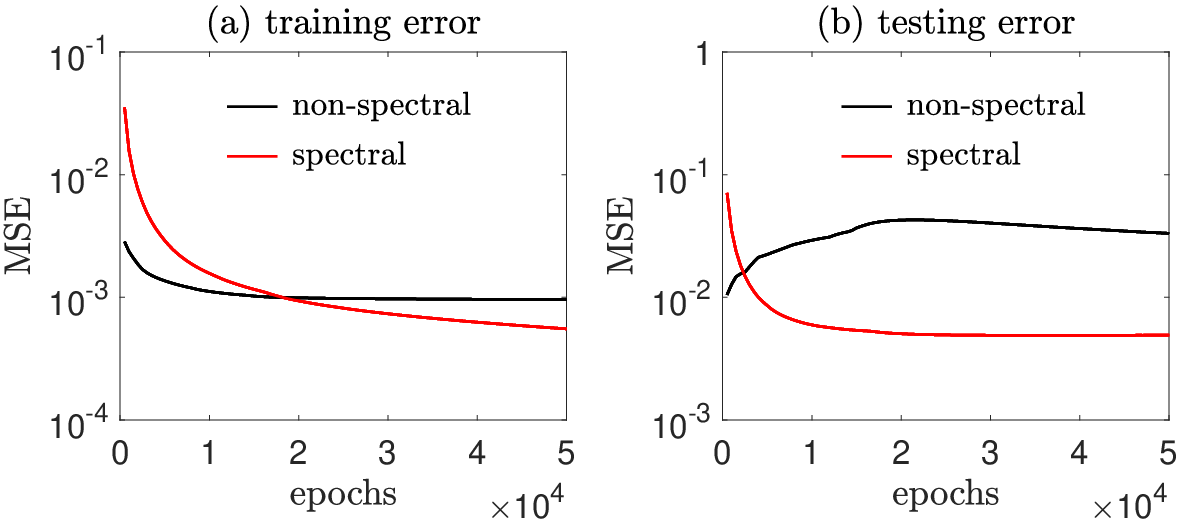
The total numbers of parameters for both the 4-layer spectral multi-output neural network and the normal 5-layer neural network are the same. The training set and the testing set each contain pairs of values where are sampled from the Cauchy distribution, , and . For each pair , we find using Eq. 3. Clearly, is sampled from the unbounded domain and cannot be normalized (the expectation and variance of the Cauchy distribution do not exist).
We set the learning rate and plot the training and testing MSEs (Eq. 4) as a function of the number of training epochs in Fig. 2. Figures 2(a) and (b) show that the spectral multi-output neural network yields smaller errors since it naturally and efficiently captures the oscillatory and decaying feature of the underlying function from Eq. 3. Directly fitting leads to over-fitting on the training set which does nothing to reduce the testing error. Therefore, it is important to take advantage of the data structure, in this case, using the spectral expansion to represent the function’s known oscillations and decay as . In this and subsequent examples, all computations are performed using Python 3.8.10 on a laptop with a 4-core Intel® i7-8550U CPU @ 1.80 GHz.
3 Application to Solving PDEs
In this section, we show that spectrally adapted neural networks can be combined with physics-informed neural networks (PINNs) which we shall call spectrally adapted PINNs (s-PINNs). We apply s-PINNs to numerically solve PDEs, and in particular, spatiotemporal PDEs in unbounded domains for which standard PINN approaches cannot be directly applied. Although we mainly focus on solving spatiotemporal problems, s-PINNs are also applicable to other types of PDEs.
Again, we assume that the problem is defined over a finite time horizon while the spatial variable may be defined in an unbounded domain. Assuming the solution’s asymptotic behavior in is known, we approximate it by a spectral expansion in with suitable basis functions (e.g., MMGFs in Example 1 for describing algebraic decay at infinity). Assuming is an operator that only involves the spatial variable (e.g., , etc.), we can represent the solution to the spatiotemporal PDE by the spectral expansion in Eq. 2 with expansion coefficients to be learned by a neural network with hyperparameters . If the solution’s behavior in both and are known and one can find proper basis functions in both the and directions, then one could use a spectral expansion in both and to solve the PDE directly without time-stepping. However, it is often the case that the time dependence is unknown and needs to be solved step-by-step in time.
As in standard PINNs, we use a high-order Runge–Kutta scheme to advance time by uniform timesteps . What distinguishes our s-PINNs from standard PINNs is that only the intermediate times between timesteps are defined as inputs to the neural network, while the outputs contain global spatial information (the spectral expansion coefficients), as shown in Fig. 1(c). Over a longer time scale, the optimal basis functions in the spectral expansion Eq. 2 may change. Therefore, one can use new adaptive spectral methods proposed in [29, 30]. Using s-PINNs to solve PDEs has the advantages that they can (i) accurately represent spatial information via spectral decomposition, (ii) convert solving a PDE into an optimization and data fitting problem, (iii) easily implement high-order, implicit schemes to advance time with high accuracy, and (iv) allow the use of recently developed spectral-adaptive techniques that dynamically find the most suitable basis functions.
The approximated solution to the PDE can be written at discrete timesteps as
| (7) |
where is the hyperparameter set of the neural network used in the time interval . In order to forward time from to , we can use, e.g., a -order implicit Runge–Kutta scheme, with () as parameters describing different collocation points in time and the associated coefficients.
Given , the -order implicit Runge–Kutta scheme aims to approximate and through
| (8) |
With the starting point defined by the initial condition at , we define the target function as the sum of squared errors
| (9) |
where the norm is taken over the spatial variable . Minimization of Eq. 9 provides a numerical solution at given its value at . If coefficients in the PDE are sufficiently smooth, we can use the basis function expansion in Eq. 7 for and find that the weights at the intermediate Runge–Kutta timesteps can be written as the Taylor expansion
| (10) |
where is the derivative of with respect to time, evaluated at . Therefore, the neural network is learning the mapping for every by minimizing the loss function Eq. 9.
Example 2
: Solving bounded domain PDEs
Before focusing on the application of s-PINNs to PDEs whose solution is
defined in an unbounded domain, we first consider the numerical
solution of a PDE in a bounded domain to compare the performance of
the spectral PINN method (using recently developed adaptive methods)
to that of the standard PINN.
Consider the following PDE:
| (11) |
which admits the analytical solution . In this example, we use Chebyshev polynomials as basis functions and the corresponding Chebyshev-Gauss-Lobatto quadrature collocation points and weights such that the boundary can be directly imposed at a collocation point .

Since the solution becomes increasingly oscillatory in over time, an ever-increasing expansion order (i.e., the number of basis functions) is needed to accurately capture this behavior. Between consecutive timesteps, we employ a recently developed -adaptive technique for tuning the expansion order [30]. This method is based on monitoring and controlling a frequency indicator defined by
| (12) |
where . The frequency indicator measures the proportion of high-frequency waves and serves as a lower error bound of the numerical solution . When exceeds its previous value by more than a factor , the expansion order is increased by one. The indicator is then updated and the factor also is scaled by a parameter .
We use a fourth-order implicit Runge–Kutta method to advance time in the SSE 9 and in order to adjust the expansion order in a timely way, we take . The initial expansion order , and the two parameters used to determine the threshold of adjusting the expansion order are set to and . A neural network with layers and neurons per layer is used in conjunction with the loss function 9 to approximate the solution of Eq. 11. We compare the results obtained using the s-PINN method with those obtained using a fourth-order implicit Runge–Kutta scheme with in a standard PINN approach [3], also using and .
Figure 3 shows that s-PINNs can be used to greatly improve accuracy because the spectral method can recover exponential convergence in space, and when combined with a high-order accurate implicit scheme in time, the overall error is small. In particular, the large error shown in Fig. 3 of the standard PINN suggests that the error of applying auto-differentiation to calculate the spatial derivative is significantly larger than the spatial derivatives calculated using spectral methods. Moreover, when equipping spectral PINNs with the -adaptive technique to dynamically adjust the expansion order, the frequency indicator can be controlled, leading to even smaller errors as shown in Fig. 3(b,c).
Computationally, using our 4-core laptop on this example, the standard PINN method requires seconds while the s-PINN approach with and without adaptive spectral techniques (dynamically increasing the expansion order ) required 1711 and 1008 seconds, respectively. Thus, s-PINN methods can be computationally more efficient than the standard PINN approach. This advantage can be better understood by noting that training of standard PINNs requires time ( is the number of neurons in the layer) to calculate each spatial derivative (e.g., ) by autodifferentiation [38]. However, in an s-PINN, since a spectral decomposition has been imposed, the computational time to calculate derivatives of all orders is , where is the expansion order. Since and the total number of neurons is usually much larger than the expansion order , using s-PINNs can substantially reduce computational cost.
What distinguishes s-PINNs from the standard PINN framework is that the latter uses spatial and temporal variables as neural-network inputs, implicitly assuming that all variables are normalizable especially when batch-normalization techniques are applied while training the underlying neural network. However, s-PINNs rely on spectral expansions to represent the dependence of a function on the spatial variable . Thus, can be defined in unbounded domains and does not need to be normalizable. In the following example, we shall explore how our s-PINN is applied to solving a PDE defined in .

.
Example 3
: Solving unbounded domain PDEs
Consider the following PDE, which is similar to Eq. 11 but
is defined in :
| (13) |
Equation 13 admits the analytical solution . In this example, we use the basis functions where is the generalized Laguerre function of order defined in [31]. Here, we use the Laguerre-Gauss quadrature collocation points and weights so that is not included in the collocation node set. We use a fourth-order implicit Runge–Kutta method to minimize the SSE 9 by advancing time. In order to address the boundary condition, we augment the loss function in Eq. 9 with terms that represent the cost of deviating from the boundary condition:
| (14) | |||
where the last two terms push the constraints associated with the Dirichlet boundary condition at at all time points:
| (15) |
where in this example, .
Because the solution of Eq. 13 becomes more diffusive with (i.e., decays more slowly at infinity), it is necessary to decrease the scaling factor to allow basis functions to decay more slowly at infinity. Between consecutive timesteps, we adjust the scaling factor by applying the scaling algorithm proposed in [29]. Thus, we dynamically adjust the basis functions in Eq. 1. As with the -adaptive technique we used in Example 2, the scaling technique also relies on monitoring and controlling the frequency indicator given in Eq. 12. In order to efficiently and dynamically tune the scaling factor, we set . The initial expansion order is , the initial scaling factor is , the scaling factor adjustment ratio is set to , and the threshold for tuning the scaling factor is set to . A neural network with 10 layers and 100 neurons per layer is used in conjunction with the loss function 9. The neural network of the standard PINN consists of eight intermediate layers with 200 neurons per layer. Figure 4(a) shows that s-PINNs can achieve very high accuracy even when a relatively large timestep () is used. Scaling techniques to dynamically control the frequency indicator are also successfully incorporated into s-PINNs, as shown in Figs. 3(b,c).
In the next example, we focus on solving a PDE with two spatial variables, and , each defined on an unbounded domain.
Example 4
: Solving 2D unbounded domain PDEs
Consider the two-dimensional heat equation on
| (16) |
which admits the analytical solution
| (17) |
Note that the solution spreads out over time in both dimensions, i.e., it decays more slowly at infinity as time increases. Therefore, we apply the scaling technique to capture the increasing spread by adjusting the scaling factors and of the generalized Hermite basis functions. Generalized Hermite functions of orders and are used in the and directions, respectively.
In order to solve Eq. 16, we multiply it by any test function and integrate the resulting equation by parts to convert it to the weak form . Solving the weak form of Eq. 16 ensures numerical stability. When implementing the spectral method, the goal is to find
| (18) |
where are generalized Hermite functions defined in Table 1 such that for all . This allows one to advance time from to given .

Tuning the scaling factors across different timesteps is achieved by monitoring the frequency indicators in the - and -directions, and , as detailed in [29]. We use initial expansion orders and scaling factors . The ratio and threshold for adjusting the scaling factors, are set to be and . The timestep is used to adjust both scaling factors in both dimensions in a timely manner and a fourth order implicit Runge–Kutta scheme is used for numerical integration. The neural network that we use to learn has 5 intermediate layers with 150 neurons in each layer.
The results depicted in Fig. 5(a) show that an s-PINN using the scaling technique can achieve high accuracy by using high-order Runge–Kutta schemes in minimizing the SSE 9 and by properly adjusting and (shown in Fig. 5(b)) to control the frequency indicators and (shown in Fig. 5(c) and (d)). The s-PINNs can be extended to higher spatial dimensions by calculating the numerical solution expressed in tensor product form as in Eq. 18.
Since our method outputs spectral expansion coefficients, if using the full tensor product in the spatial spectral decomposition leads to a number of outputs that increase exponentially with dimensionality. The very wide neural networks needed for such high-dimensional problems results in less efficient training. However, unlike other recent machine–learning–based PDE solvers or PDE learning methods [39, 40] that explicitly rely on a spatial discretization of grids or meshes, the curse of dimensionality can be partially mitigated in our s-PINN method. By using a hyperbolic cross space [41], we can effectively reduce the number of coefficients needed to accurately reconstruct the numerical solution. In the next example, we solve a 3D parabolic spatiotemporal PDE, similar to that in Example 4, but we demonstrate how implementing a hyperbolic cross space can reduce the number of outputs and boost training efficiency.
Example 5
: Solving 3D unbounded domain PDEs
Consider the (3+1)-dimensional heat equation
| (19) |
which admits the analytical solution
| (20) |
for . If we use the full tensor product of spectral expansions with expansion orders , we will need to output expansion coefficients, and in turn, a relatively wide neural network with many parameters will be needed to generate the corresponding weights as shown in Fig. 1(c). Training such wide networks can be inefficient. However, many of the spectral expansion coefficients are close to zero and can be eliminated without compromising accuracy. One way to select expansion coefficients is to use the hyperbolic cross space technique [41] to output coefficients of the generalized Hermite basis functions only in the space
| (21) |
where the hyperbolic space index . Taking in Eq. 21 corresponds to the full tensor product with basis functions in each dimension. For fixed in Eqs. 21, the number of total basis function tend to decrease with increasing . We set in Eq. 21 and use the initial scaling factors . Using a fourth-order implicit Runge–Kutta scheme with timestep , we set the ratio and threshold for adjusting the scaling factors are set to and in each dimension.
To illustrate the potential numerical difficulties arising from outputting large numbers of coefficients when solving higher-dimensional spatiotemporal PDEs, we use a neural network with two hidden layers and different numbers of neurons in the intermediate layers. We also adjust to explore how decreasing the number of coefficients can improve training efficiency. Our results are listed Table 2.
| 0 | ||||
| 200 | ||||
| 400 | ||||
| 700 | ||||
| 1000 |
The results shown in Table 2 indicate that, compared to using the full tensor product , implementing the hyperbolic cross space with a moderate or , the total number of outputs is significantly reduced, leading to faster training and better accuracy. However, increasing the hyperbolicity to , the error increases relative to using because some useful, nonzero coefficients are excluded. Also, comparing the results across different rows, wider layers lead to both more accurate results and faster training speed. The sensitivity of our s-PINN method to the number of intermediate layers in the neural network and the number of neurons in each layer are further discussed in Example 7. Overall, in higher-dimensional problems, there is a balance between computational cost and accuracy as the number of outputs needed will grow fast with dimensionality. Spectrally-adapted PINNs can easily incorporate a hyperbolic cross space so that the total number of outputs can be reduced to a manageable number for moderate-dimensional problems. Finding the optimal hyperbolicity index for the cross space Eq. 21 will be problem-specific.
In the next example, we explore how s-PINNs can be used to solve Schrödinger’s equation in . Solving this complex-valued equation poses substantial numerical difficulties as the solution exhibits diffusive, oscillatory, and convective behavior [24].
Example 6
: Solving an unbounded domain Schrödinger equation
We seek to numerically solve the following Schrödinger equation
defined on
| (22) |
For reference, Eq. 22 admits the analytical solution
| (23) |
As in Example 4, we shall numerically solve Eq. 22 in the weak form
| (24) |
Since the solution to Eq. 22 decays as at infinity, we shall use the generalized Hermite functions as basis functions. The solution is rightward-translating for and increasingly oscillatory and spread out over time. Hence, as detailed in [30], we apply three additional adaptive spectral techniques to improve efficiency and accuracy: (i) a scaling technique to adjust the scaling factor over time in order to capture diffusive behavior, (ii) a moving technique to adjust the center of the basis function to capture convective behavior, and (iii) a -adaptive technique to increase the number of basis functions to better capture the oscillations. We set the initial parameters at . The scaling factor adjustment ratio and the threshold for adjusting the scaling factor are , the minimum and maximum displacements are and within each timestep for moving the basis functions, respectively, and the threshold for moving is . Finally, the thresholds of the -adaptive technique are set to and . To numerically solve Eq. 24, a fourth-order implicit Runge–Kutta scheme is applied to advance time with timestep . The neural network underlying the s-PINN that we use in this example contains 13 layers with 80 neurons in each layer.

Figure 6(a) shows that the s-PINN with adaptive spectral techniques leads to very high accuracy as it can properly adjust the basis functions over a longer timescale (across different timesteps), while not adapting the basis functions results in larger errors. Figs. 6(b–d) show that the scaling factor decreases over time to match the spread of the solution, the displacement of the basis function increases in time to capture the rightward movement of the basis functions, and the expansion order increases to capture the solution’s increasing oscillatory behavior. Our results indicate that our s-PINN method can effectively utilize all three adaptive algorithms.
We now explore how the timestep and the order of the implicit Runge–Kutta method affect the approximation error, i.e., to what extent can we relax the constraint on the timestep and maintain the accuracy of the basis functions, or, if higher-order Runge–Kutta schemes are better. Another feature to explore is the neural network structure, such as the number of layers and neurons per layer, and how it affects the performance of s-PINNs. In the following example, we carry out a sensitivity analysis.
Example 7
: Sensitivity analysis of s-PINN
To explore how the performance of an s-PINN depends on algorithmic
set-up and parameters, we apply it to solving the heat equation
defined on ,
| (25) |
using generalized Hermite functions as basis functions. For the source , Eq. 25 admits the analytical solution
| (26) |
We solve Eq. 25 in the weak form by multiplying any test function on both sides and integrating by parts to obtain
| (27) |
The solution diffusively spreads over time, requiring one to decrease the scaling factor of the generalized Hermite functions . We shall first study how the timestep and the order of the implicit Runge–Kutta method associated with solving the minimization problem 9 affect our results. We use a neural network with five intermediate layers and 200 neurons per layer, and set the learning rate . The initial scaling factor is set to . The scaling factor adjustment ratio and threshold are set to , and , respectively. For comparison, we also apply a Crank-Nicolson scheme for numerically solving Eq. 27, i.e.,
| (28) |
where are the -dimensional vectors of spectral expansion coefficients of the numerical solution and the of the source, respectively. is the tridiagonal block matrix representing the discretized Laplacian operator :
and , otherwise.
| C-K scheme | 2 | 4 | 6 | 10 | |
| 0.02 | 12, 8.252e-06, 0.545 | 27, 4.011e-08, 0.545 | 54, 1.368e-08, 0.545 | 279, 2.545e-07, 0.545 | 7071, 6.358e-05, 0.695 |
| 0.05 | 5, 5.157e-05, 0.545 | 12, 2.799e-08, 0.545 | 23, 1.651e-08, 0.545 | 105, 2.566e-07, 0.545 | 3172, 1.052e-06, 0.545 |
| 0.1 | 3, 2.239e-04, 0.695 | 6, 1.331e-06, 0.695 | 10, 1.314e-06, 0.695 | 72, 1.346e-06, 0.695 | 1788, 2.782e-06, 0.695 |
| 0.2 | 2, 9.308e-04, 0.695 | 3, 3.760e-06, 0.695 | 9, 2.087e-06, 0.695 | 317, 2.107e-06, 0.695 | 1310, 1.925e-03, 0.753 |
Table 3 shows that since the error from temporal discretization is already quite small for , using a higher-order Runge–Kutta method does not significantly improve accuracy for all choices of . Using higher-order () schemes tends to require longer run times. Higher orders require fitting over more data points (using the same number of parameters) leading to slower convergence when minimizing Eq. 9, which can result in larger errors. Compared to the second-order Crank-Nicolson scheme, whose error is , the errors of our s-PINN method do not grow significantly when increases. In fact, the accuracy using the smallest timestep in the Crank-Nicolson scheme was still inferior to that of the s-PINN method using the second order or fourth order Runge-Kutta scheme with . Moreover, the run time of our s-PINN method using a second or fourth-order implicit Runge–Kutta scheme for the loss function is not significantly larger than that of the Crank-Nicolson scheme. Thus, compared to traditional spectral methods for numerically solving PDEs, our s-PINN method, even when incorporating some lower-order Runge–Kutta schemes, can greatly improve accuracy without significantly increasing computational cost.
In Table 3, the smallest run time of our s-PINN method, which occurs for , is shown in blue. The smallest error case, which arises for , is shown in red. The run time always increases with the order of the implicit Runge–Kutta scheme and always decreases with due to fewer timesteps. Additionally, the error always increases with regardless of the order of the Runge–Kutta scheme. However, the expected convergence order is not observed, implying that the increase in error results from increased lag in adjustment of the scaling factor when is too large, rather than from an insufficiently small time discretization error . Using a fourth-order implicit Runge–Kutta scheme with to solve Eq. 27 seems to both achieve high accuracy and avoid large computational costs.
We also investigate how the total number of parameters in the neural network and the structure of the network affect efficiency and accuracy. We use a sixth-order implicit Runge–Kutta scheme with . The learning rate is set to for all neural networks.
| 3 | 5 | 8 | 13 | |
| 50 | 1348, 6.317e-04, 0.738 | 798, 9.984e-05, 0.695 | 995, 1.891e-04, 0.579 | 778, 4.022e-04, 0.695 |
| 80 | 784, 7.164e-04, 0.654 | 234, 1.349e-06, 0.695 | 216, 1.345e-06, 0.695 | 376, 1.982e-06, 0.695 |
| 100 | 1080, 8.804e-05, 0.695 | 114, 1.344e-06, 0.695 | 102, 1.346e-06, 0.695 | 145, 1.348e-06, 0.695 |
| 200 | 219, 1.349e-06, 0.695 | 72, 1.346e-06, 0.695 | 43, 1.347e-06, 0.695 | 64, 1.345e-06, 0.695 |
As shown in Table 4, the computational cost tends to decrease with the number of neurons in each layer as it takes fewer epochs to converge when minimizing Eq. 9. The run time tends to decrease with due to a faster convergence rate, until about . The errors when are significantly larger as the training terminates (after a maximum of 100000 epochs) before it converges. For , the corresponding s-PINN always fails to achieve accuracy within 100000 epochs unless . Therefore, overparametrization is indeed helpful in improving the neural network’s performance, leading to faster convergence rates, in contrast to most traditional optimization methods that take longer to converge with more parameters. Similar observations have been made in other optimization tasks that involve deep neural networks [42, 43]. Consequently, our s-PINN method retains the advantages of deep and wide neural networks for improving accuracy and efficiency.
4 Parameter Inference and Source Reconstruction
As with standard PINN approaches, s-PINNs can also be used for parameter inference in PDE models or reconstructing unknown sources in a physical model. Assuming observational data at uniform time intervals associated with a partially known underlying PDE model, s-PINNs can be trained to infer model parameters by minimizing the sum of squared errors, weighted from both ends of the time interval ,
| (29) |
where
| (30) | |||||
Here, is the model parameter to be found using the sample points between and . The most obvious advantage of s-PINNs over standard PINN methods is that they can deal with models defined on unbounded domains, extending PINN-based methods that are typically applied to finite domains.
Given observations over a certain time interval, one may wish to both infer parameters in the underlying physical model and reconstruct the solution at any given time. Here, we provide an example in which both a parameter in the model is to be inferred and the numerical solution obtained.
Example 8
: Parameter (diffusivity) inference
As a starting point for a parameter-inference problem, we consider
diffusion with a source defined on
| (31) |
where the constant parameter is the thermal conductivity (or diffusion coefficient) in the entire domain. In this example, we set as a reference and assume the source
| (32) |
In this case, the analytical solution to Eq. 31 is given by Eq. 26. We numerically solve Eq. 31 in the weak form of Eq. 27. If the form of the spatiotemporal heat equation is known (such as Eq. 31), but some parameters such as is unknown, reconstructing it from measurements is usually performed by defining and minimizing a loss function as was done in [44]. It can also be shown that in Eq. 31 can be uniquely determined by the observed solution [45, 46, 47] under certain conditions. Here, however, we assume that observations are taken at discrete time points and seek to reconstruct both the parameter and the numerical solution at (defined in Eqs. 30) by minimizing Eq. 29. We use a neural network with 13 layers and 100 neurons per layer with a sixth-order implicit Runge–Kutta scheme. The timestep is 0.1. At each timestep, we draw the function values from
| (33) |
where is the noise term that is both spatially and temporally uncorrelated, and , where is the normal distribution of mean 0 and variance (i.e., ). For different levels of noise , we take one trajectory of the measured solution with noise to reconstruct the parameter , which is presumed to be a constant in , and simultaneously obtain the numerical solutions at the intermediate time points . We are interested in how different levels of noise and the increasing spread of the solution will affect the SSE and the reconstructed parameter . Figure 7 shows the deviation of the reconstructed from its true value, , the SSE, the scaling factor, and the frequency indicator as functions of time for different noise levels.
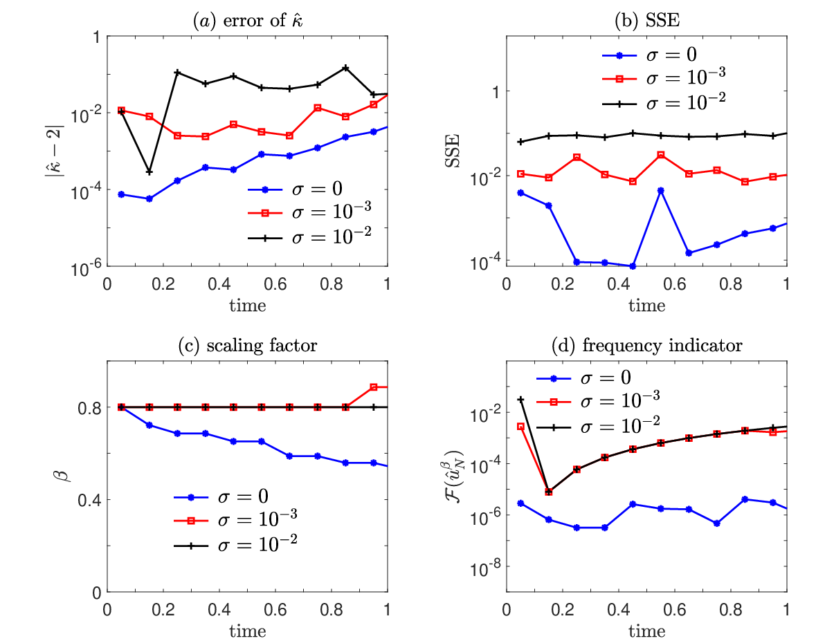
Figure 7(a) shows that the larger the noise, the less accurate the reconstructed . Moreover, as the function becomes more spread out (when ), the error in both the reconstructed diffusivity and the SSE increases across time, as shown in Fig. 7(b). This behavior suggests that a diffusive solution that decays more slowly at infinity can give rise to inaccuracies in the numerical computation of the intermediate timestep solutions and in reconstructing model parameters. Finally, as indicated in Fig. 7(c,d), larger variances in the noise will impede the scaling process since the frequency indicator cannot be as easily controlled because larger variance in the noise usually corresponds to high-frequency and oscillatory components of a solution.
In Example 8, both the parameter and the unknown solution were inferred. Apart from reconstructing the coefficients in a given physical model, in certain applications, we may also wish to reconstruct the underlying physical model by inferring, e.g., the heat source . Source recovery from observational data commonly arises and has been the subject of many previous studies [48, 49, 50]. We now discuss how the s-PINN methods presented here can also be used for this purpose. For example, in Eq. 25 or Eq. 31, we may wish to reconstruct an unknown source by also approximating it with a spectral decomposition
| (34) |
and minimizing an SSE that is augmented by a penalty on the coefficients .
We learn the expansion coefficients within by minimizing
| (35) | |||||
where and (or the spectral expansion coefficients of ) is assumed known at all intermediate time points in .
The last term in Eq. 35 adds an penalty term on the coefficients of which tends to reconstruct smoother and smaller-magnitude sources as is increased. Other forms of regularization such as can also be considered [51]. In the presence of noise, an regularization further drives small expansion weights to zero, yielding an inferred source described by fewer nonzero weights.
Since the reconstructed heat source is expressed in terms of a spectral expansion in Eq. 34, and minimizing the loss function Eq. 35 depends on the global information of the observation , at any location also contains global information intrinsic to . In other words, for such inverse problems, the s-PINN approach extracts global spatial information and is thus able to reconstruct global quantities. We consider an explicit case in the next example.
Example 9
: Source recovery
Consider the canonical source reconstruction problem
[52, 53, 54]
of finding in the heat equation model in
Eq. 25 for which observational data are given by
Eq. 33 but evaluated at . A
physical interpretation of the reconstruction problem is identifying
the heat source using measurement data in conjunction with
Eq. 25. As in Example 5, we numerically solve the weak
form Eq. 27. To study how the penalty term in
Eq. 35 affect source recovery and whether
increasing the regularization will make the inference of
more robust against noise, we minimize Eq. 29 for
different values of and .
| 0 | ||||
| 0 | ||||
We use a neural network with 13 layers and 100 neurons per layer to reconstruct in the decomposition Eq. 34 with , i.e., the neural network outputs the coefficients at the intermediate timesteps . The basis functions are chosen to be Hermite functions . For simplicity, we consider the problem only at times within the first time point and a fixed scaling factor as well as a fixed displacement .
In Table 5, we record the error
| (36) |
the lower-left of each entry and the in the upper-right. Observe that as the variance of the noise increases, the reconstruction of via the spectral expansion becomes increasingly inaccurate.
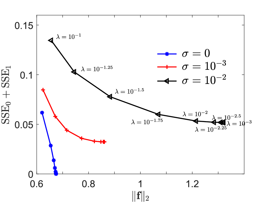
In the noise-free case, taking in Eq. 35 achieves the smallest and the smallest reconstruction error. However, with increasing noise , using an regularization term in Eqs. 35 can prevent over-fitting of the data although increases with the regularization strength . When , taking achieves the smallest reconstruction error Eq. 36; when , achieves the smallest reconstruction error. However, if is too large, coefficients of the spectral approximation to are pushed to zero. Thus, it is important to choose an intermediate so that the reconstruction of the source is robust to noise. In Fig. 8, we plot the norm of the reconstructed heat source and the “error” which varies as changes for different .
5 Summary and Conclusions
In this paper, we propose an approach that blends standard PINN algorithms with adaptive spectral methods and show through examples that this hybrid approach can be applied to a wide variety of data-driven problems including function approximation, solving PDEs, parameter inference, and model selection. The underlying feature that we exploit is the physical differences across classes of data. For example, by understanding the difference between space and time variables in a PDE model, we can describe the spatial dependence in terms of basis functions, obviating the need to normalize spatial data. Thus, s-PINNs are ideal for solving problems in unbounded domains. The only additional “prior” needed is an assumption on the asymptotic spatial behavior and an appropriate choice of basis functions. Additionally, adaptive techniques have been recently developed to further improve the efficiency and accuracy, making spectral decomposition especially suitable for unbounded-domain problems that the standard PINN cannot easily address.
We applied s-PINNs (exploiting adaptive spectral methods) across a number of examples and showed that they can outperform simple neural networks for function approximation and existing PINNs for solving certain PDEs. Three major advantages are that s-PINNs can be applied to unbounded domain problems, more accurate by recovering spectral convergence in space, and more efficient as a result of faster evaluation of spatial derivatives of all orders compared to standard PINNs that use autodifferentiation. These advantages are rooted in separated data structures, allowing for spectral computation and high-accuracy numerics. Straightforward implementation of s-PINNs retains most of the advantageous features of deep-neural-network in PINNs, making s-PINNs ideal for data-driven inference problems. However, in the context of solving higher-dimensional PDEs, a tradeoff is necessary when using s-PINNs instead of PINNs. For s-PINNs, the network structure needs to be significantly widened to output an exponentially increasing (with dimensionality) number of expansion coefficients, while in standard PINNs, the network structure remains largely preserved but an exponentially larger number of trajectories are needed for sufficient training. We found that by restricting the spatial domain to a hyperbolic cross space, the number of outputs required for s-PINNs can be appreciably decreased for problems of moderate dimensions. While using a hyperbolic cross space cannot reduce the number of outputs sufficiently to allow s-PINNs to be effective for very high dimensional problems, the standard PINNs approach to problems in very high dimensions could require an unattainable number of samples for sufficient training.
In Table 6, we compare the advantages and disadvantages of the standard PINN and s-PINN methods. Potential improvements and extensions include applying techniques for selecting basis functions that best characterize the expected underlying process, spatial or otherwise, and inferring forms of the underlying model PDEs [55, 56]. While standard PINN methods deal with local information (e.g., ), spectral decompositions capture global information making them a natural choice for also efficiently learning and approximating nonlocal terms such as convolutions and integral kernels. Potential future exploration using our s-PINN method may include adapting it to solve higher-dimensional problems by more systematically choosing a proper hyperbolic space or using other coefficient-reducing (outputs of the neural network) techniques. Also, recent Gaussian–process–based smoothing techniques [57] can be considered to improve robustness of our s-PINN method against noise/errors in measurements, and noise-aware physics-informed machine learning techniques [58] can be incorporated when applying our s-PINN for inverse-type PDE discovery problems. Finally, one can incorporate a recently proposed Bayesian-PINN (B-PINN) [59] method into our s-PINN method to quantify uncertainty when solving inverse problems under noisy data.
| Traditional | PINN | |
| Non-spectral | + leverages existing numerical methods + low-order FD/FE schemes easily implemented + efficient evaluation of function and derivatives – mainly restricted to bounded domains – complicated time-extrapolation – complicated implementation of higher-order schemes – algebraic convergence, less accurate – more complicated inverse-type problems – more complicated temporal and spatial extrapolation – requires understanding of problem to choose suitable discretization | + easy implementation + efficient deep-neural-network training + easy extrapolation + easily handles inverse-type problems – mainly restricted to bounded domains – less accurate – less interpretable spatial derivatives – limited control of spatial discretization – expensive evaluation of neural networks – incompatible with existing numerical methods |
| Spectral | + suitable for bounded and unbounded domains + spectral convergence in space, more accurate + leverage existing numerical methods + efficient evaluation of function and derivatives – information required for choosing basis functions – more complicated inverse-type problems – more complicated implementation – more complicated temporal extrapolation in time – usually requires a “regular” domain e.g. rectangle, , a ball, etc. | + suitable for both bounded and unbounded domains + easy implementation + spectral convergence in space, more accurate + efficient deep-neural-network training + more interpretable derivatives of spatial variables + easy extrapolation + easily handles inverse-type problems + compatible with existing adaptive techniques – requires some information to choose basis functions – expensive evaluation of neural networks – usually requires a “regular” domain |
References
- [1] Kurt Hornik. Approximation capabilities of multilayer feedforward networks. Neural Networks, 4(2):251–257, 1991.
- [2] Sejun Park, Chulhee Yun, Jaeho Lee, and Jinwoo Shin. Minimum width for universal approximation. In International Conference on Learning Representations, 2020.
- [3] Maziar Raissi, Paris Perdikaris, and George E Karniadakis. Physics-informed neural networks: A deep learning framework for solving forward and inverse problems involving nonlinear partial differential equations. Journal of Computational Physics, 378:686–707, 2019.
- [4] George Em Karniadakis, Ioannis G Kevrekidis, Lu Lu, Paris Perdikaris, Sifan Wang, and Liu Yang. Physics-informed machine learning. Nature Reviews Physics, 3(6):422–440, 2021.
- [5] Thomas Asikis, Lucas Böttcher, and Nino Antulov-Fantulin. Neural ordinary differential equation control of dynamics on graphs. Physical Review Research (in press), 2022.
- [6] Lucas Böttcher, Nino Antulov-Fantulin, and Thomas Asikis. AI Pontryagin or how neural networks learn to control dynamical systems. Nature Communications, 2021.
- [7] Lucas Böttcher and Thomas Asikis. Near-optimal control of dynamical systems with neural ordinary differential equations. Machine Learning: Science and Technology, 3(4):045004, 2022.
- [8] FW Lewis, Suresh Jagannathan, and Aydin Yesildirak. Neural network control of robot manipulators and non-linear systems. CRC Press, 2020.
- [9] Jan Kukačka, Vladimir Golkov, and Daniel Cremers. Regularization for deep learning: A taxonomy. arXiv preprint arXiv:1710.10686, 2017.
- [10] M Lutter, C Ritter, and Jan Peters. Deep Lagrangian networks: Using physics as model prior for deep learning. In International Conference on Learning Representations. OpenReview.net, 2019.
- [11] Manuel A Roehrl, Thomas A Runkler, Veronika Brandtstetter, Michel Tokic, and Stefan Obermayer. Modeling system dynamics with physics-informed neural networks based on Lagrangian mechanics. IFAC-PapersOnLine, 53(2):9195–9200, 2020.
- [12] Yaofeng Desmond Zhong, Biswadip Dey, and Amit Chakraborty. Symplectic ODE-net: Learning Hamiltonian dynamics with control. In International Conference on Learning Representations, 2019.
- [13] Ehsan Kharazmi, Zhongqiang Zhang, and George Em Karniadakis. Variational physics-informed neural networks for solving partial differential equations. arXiv preprint arXiv:1912.00873, 2019.
- [14] Ameya D Jagtap and George Em Karniadakis. Extended physics-informed neural networks (xpinns): A generalized space-time domain decomposition based deep learning framework for nonlinear partial differential equations. Communications in Computational Physics, 28(5):2002–2041, 2020.
- [15] Zongyi Li, Hongkai Zheng, Nikola Kovachki, David Jin, Haoxuan Chen, Burigede Liu, Kamyar Azizzadenesheli, and Anima Anandkumar. Physics-informed neural operator for learning partial differential equations. arXiv preprint arXiv:2111.03794, 2021.
- [16] Zhiping Mao, Ameya D Jagtap, and George Em Karniadakis. Physics-informed neural networks for high-speed flows. Computer Methods in Applied Mechanics and Engineering, 360:112789, 2020.
- [17] Zhiwei Fang and Justin Zhan. A physics-informed neural network framework for PDEs on 3D surfaces: Time independent problems. IEEE Access, 8:26328–26335, 2019.
- [18] George S Misyris, Andreas Venzke, and Spyros Chatzivasileiadis. Physics-informed neural networks for power systems. In 2020 IEEE Power & Energy Society General Meeting (PESGM), pages 1–5. IEEE, 2020.
- [19] Francisco Sahli Costabal, Yibo Yang, Paris Perdikaris, Daniel E Hurtado, and Ellen Kuhl. Physics-informed neural networks for cardiac activation mapping. Frontiers in Physics, 8:42, 2020.
- [20] Minliang Liu, Liang Liang, and Wei Sun. A generic physics-informed neural network-based constitutive model for soft biological tissues. Computer methods in applied mechanics and engineering, 372:113402, 2020.
- [21] Lucas Böttcher and Hans J Herrmann. Computational Statistical Physics. Cambridge University Press, 2021.
- [22] Stefan H Strub and Lucas Böttcher. Modeling deformed transmission lines for continuous strain sensing applications. Measurement Science and Technology, 31(3):035109, 2019.
- [23] Julien Barré, Alain Olivetti, and Yoshiyuki Y Yamaguchi. Algebraic damping in the one-dimensional Vlasov equation. Journal of Physics A: Mathematical and Theoretical, 44(40):405502, 2011.
- [24] Buyang Li, Jiwei Zhang, and Chunxiong Zheng. Stability and error analysis for a second-order fast approximation of the one-dimensional Schrödinger equation under absorbing boundary conditions. SIAM Journal on Scientific Computing, 40(6):A4083–A4104, 2018.
- [25] Mingtao Xia, Chris D Greenman, and Tom Chou. PDE models of adder mechanisms in cellular proliferation. SIAM Journal on Applied Mathematics, 80(3):1307–1335, 2020.
- [26] Mingtao Xia and Tom Chou. Kinetic theory for structured populations: application to stochastic sizer-timer models of cell proliferation. Journal of Physics A: Mathematical and Theoretical, 2021.
- [27] Elena Mengotti, Laura J Heyderman, Arantxa Fraile Rodríguez, Frithjof Nolting, Remo V Hügli, and Hans-Benjamin Braun. Real-space observation of emergent magnetic monopoles and associated Dirac strings in artificial Kagomé spin ice. Nature Physics, 7(1):68–74, 2011.
- [28] RV Hügli, G Duff, B O’Conchuir, E Mengotti, A Fraile Rodríguez, F Nolting, LJ Heyderman, and HB Braun. Artificial Kagomé spin ice: dimensional reduction, avalanche control and emergent magnetic monopoles. Philosophical Transactions of the Royal Society A: Mathematical, Physical and Engineering Sciences, 370(1981):5767–5782, 2012.
- [29] Mingtao Xia, Sihong Shao, and Tom Chou. Efficient scaling and moving techniques for spectral methods in unbounded domains. SIAM Journal on Scientific Computing, 43(5):A3244–A3268, 2021.
- [30] Mingtao Xia, Sihong Shao, and Tom Chou. A frequency-dependent p-adaptive technique for spectral methods. Journal of Computational Physics, 446:110627, 2021.
- [31] Jie Shen, Tao Tang, and Li-Lian Wang. Spectral methods: algorithms, analysis and applications, volume 41. Springer Science & Business Media, 2011.
- [32] Lloyd N Trefethen. Spectral methods in MATLAB. SIAM, 2000.
- [33] Seppo Linnainmaa. Taylor expansion of the accumulated rounding error. BIT Numerical Mathematics, 16(2):146–160, 1976.
- [34] Adam Paszke, Sam Gross, Soumith Chintala, Gregory Chanan, Edward Yang, Zachary DeVito, Zeming Lin, Alban Desmaison, Luca Antiga, and Adam Lerer. Automatic differentiation in PyTorch. 2017.
- [35] Kurt Hornik, Maxwell Stinchcombe, and Halbert White. Multilayer feedforward networks are universal approximators. Neural Networks, 2(5):359–366, 1989.
- [36] Sergey Ioffe and Christian Szegedy. Batch normalization: Accelerating deep network training by reducing internal covariate shift. In International Conference on Machine Learning, pages 448–456. PMLR, 2015.
- [37] Tao Tang, Li-Lian Wang, Huifang Yuan, and Tao Zhou. Rational spectral methods for PDEs involving fractional Laplacian in unbounded domains. SIAM Journal on Scientific Computing, 42(2):A585–A611, 2020.
- [38] Atilim Gunes Baydin, Barak A Pearlmutter, Alexey Andreyevich Radul, and Jeffrey Mark Siskind. Automatic differentiation in machine learning: a survey. Journal of Machine Learning Research, 18, 2018.
- [39] Johannes Brandstetter, Daniel E Worrall, and Max Welling. Message passing neural PDE solvers. In International Conference on Learning Representations, 2021.
- [40] Zongyi Li, Nikola Borislavov Kovachki, Kamyar Azizzadenesheli, Kaushik Bhattacharya, Andrew Stuart, Anima Anandkumar, et al. Fourier neural operator for parametric partial differential equations. In International Conference on Learning Representations, 2020.
- [41] Jie Shen and Li-Lian Wang. Sparse spectral approximations of high-dimensional problems based on hyperbolic cross. SIAM Journal on Numerical Analysis, 48(3):1087–1109, 2010.
- [42] Sanjeev Arora, Nadav Cohen, and Elad Hazan. On the optimization of deep networks: Implicit acceleration by overparameterization. In Jennifer Dy and Andreas Krause, editors, Proceedings of the 35th International Conference on Machine Learning, volume 80 of Proceedings of Machine Learning Research, pages 244–253, 2018.
- [43] Zixiang Chen, Yuan Cao, Difan Zou, and Quanquan Gu. How much over-parameterization is sufficient to learn deep ReLU networks? In International Conference on Learning Representations, 2020.
- [44] Mousa J. Huntul. Identification of the timewise thermal conductivity in a 2D heat equation from local heat flux conditions. Inverse Problems in Science and Engineering, 29(7):903–919, 2021.
- [45] NI Ivanchov. Inverse problems for the heat-conduction equation with nonlocal boundary conditions. Ukrainian Mathematical Journal, 45(8):1186–1192, 1993.
- [46] B Frank Jones Jr. The determination of a coefficient in a parabolic differential equation: Part i. existence and uniqueness. Journal of Mathematics and Mechanics, pages 907–918, 1962.
- [47] N. Ya. Beznoshchenko. On finding a coefficient in a parabolic equation. Differential Equations, 10:24–35, 1974.
- [48] Liang Yan, Feng-Lian Yang, and Chu-Li Fu. A meshless method for solving an inverse spacewise-dependent heat source problem. Journal of Computational Physics, 228(1):123–136, 2009.
- [49] Liu Yang, Mehdi Dehghan, Jian-Ning Yu, and Guan-Wei Luo. Inverse problem of time-dependent heat sources numerical reconstruction. Mathematics and Computers in Simulation, 81(8):1656–1672, 2011.
- [50] Fan Yang and Chu-Li Fu. A simplified Tikhonov regularization method for determining the heat source. Applied Mathematical Modelling, 34(11):3286–3299, 2010.
- [51] Tailin Wu and Max Tegmark. Toward an artificial intelligence physicist for unsupervised learning. Physical Review E, 100(3):033311, 2019.
- [52] John Rozier Cannon. Determination of an unknown heat source from overspecified boundary data. SIAM Journal on Numerical Analysis, 5(2):275–286, 1968.
- [53] B Tomas Johansson and Daniel Lesnic. A variational method for identifying a spacewise-dependent heat source. IMA Journal of Applied Mathematics, 72(6):748–760, 2007.
- [54] Alemdar Hasanov and Burhan Pektacc. A unified approach to identifying an unknown spacewise dependent source in a variable coefficient parabolic equation from final and integral overdeterminations. Applied Numerical Mathematics, 78:49–67, 2014.
- [55] Zichao Long, Yiping Lu, Xianzhong Ma, and Bin Dong. PDE-net: Learning PDEs from data. In International Conference on Machine Learning, pages 3208–3216. PMLR, 2018.
- [56] Maziar Raissi. Deep hidden physics models: Deep learning of nonlinear partial differential equations. Journal of Machine Learning Research, 19(1):932–955, 2018.
- [57] Chandrajit Bajaj, Luke McLennan, Timothy Andeen, and Avik Roy. Recipes for when physics fails: Recovering robust learning of physics informed neural networks. Machine Learning: Science and Technology, 2023.
- [58] Pongpisit Thanasutives, Takashi Morita, Masayuki Numao, and Ken-ichi Fukui. Noise-aware physics-informed machine learning for robust pde discovery. Machine Learning: Science and Technology, 4:015009, 2022.
- [59] Liu Yang, Xuhui Meng, and George Em Karniadakis. B-PINNs: Bayesian physics-informed neural networks for forward and inverse PDE problems with noisy data. Journal of Computational Physics, 425:109913, 2021.