Stable factorization for phase factors of quantum signal processing

This paper is concerned with the problem of quantum signal processing. Quantum computing has been mostly working with unitary operators, since the quantum gates and circuits are unitary. However, in recent years, we have witnessed great progress in representing non-unitary operators efficiently with quantum circuits.

Let $A$ be an $N\times N$ Hermitian matrix with $N=2^{n}$ and $\|A\|_{2}<1$ (after scaling if needed). For simplicity, we only consider Hermitian matrices in this paper and refer the readers to [6, 4] for more general cases. One of the most successful methods for presenting $A$ on a quantum circuit is the Hermitian block encoding

where $U_{A}$ is a Hermitian unitary matrix of size $(2^{m}\cdot N)\times(2^{m}\cdot N)$, $A$ is the top-left corner of $U_{A}$, and $U_{A}$ can be implemented using a quantum circuit with $n+m$ input qubits.

In most of the quantum problems in scientific computing, such as Hamiltonian simulation, filtering, and quantum linear algebra [3, 10, 4, 13], one is often interested the Hermitian matrix $f(A)$ of $A$, where $f(x)$ is a real function defined on $[-1,1]$ with $\|f\|_{\infty}<1$. The block encoding scheme requires $f(A)$ to be represented as the top-left block of a larger unitary matrix $U_{f(A)}$ implemented by a quantum circuit

A key question is whether there is an algorithm that builds the quantum circuit $U_{f(A)}$ from the circuit $U_{A}$ by using only the knowledge of the function $f(x)$ but treating $U_{A}$ as a black box

This question is answered by the quantum eigenvalue transformation described in [9, 6]. To simplify the discussion, we assume that all Hermitian matrices mentioned below satisfy $\|A\|_{2}<1$ and all functions defined on $[-1,1]$ satisfy $\|f\|_{\infty}<1$. The quantum eigenvalue transform proceeds as follows (see [8] for example for details).

• •

  Split the polynomial $f(x)$ into the even and odd parts $f^{\text{e}}(x)$ and $f^{\text{o}}(x)$ on $x\in[-1,1]$

• •

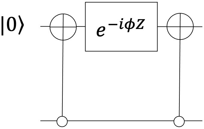
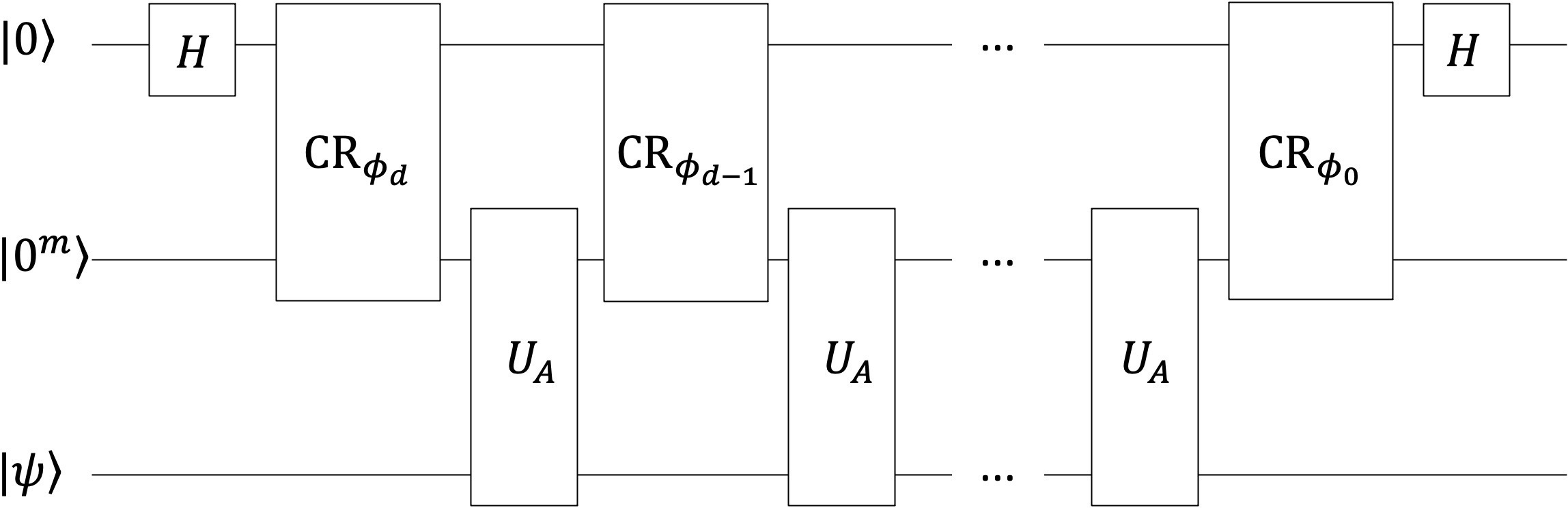
  Approximate the even part $f^{\text{e}}(x)$ with an even degree polynomial $a^{\text{e}}(x)$ and implement $a_{\text{e}}(A)$ with a circuit shown in Figure 1(b) with appropriate phase factors $\phi^{\text{e}}_{0},\ldots,\phi^{\text{e}}_{d_{\text{e}}}$. Here $d_{\text{e}}$ is the equal to degree of $a^{\text{e}}(x)$.

• •

  Approximate the odd part $f^{\text{o}}(x)$ with an odd degree polynomial $a^{\text{o}}(x)$ and implement $a_{\text{o}}(A)$ with a circuit shown in Figure 1(b) with appropriate phase factors $\phi^{\text{o}}_{0},\ldots,\phi^{\text{o}}_{d_{\text{o}}}$. Here $d_{\text{o}}$ is the equal to degree of $a^{\text{o}}(x)$.

• •

  Combine the circuits implementing each component together by linear combination of unitaries (LCU) [2].

The key remaining step is how to construct the phase factors $\phi_{0},\ldots,\phi_{d}$ for an even or odd polynomial $a(x)$ of degree $d$. This is answered by the quantum signal processing theorem [9, 6, 10]: Given a polynomial $a(x)\in\mathbb{R}[x]$ on $[-1,1]$ of degree $d$, parity $d\mod 2$, and $\|a\|_{\infty}=\max_{x\in[-1,1]}|a(x)|<1$, there exists a sequence of phase factors $\Phi=(\phi_{0},\ldots,\phi_{d})\in[-\pi,\pi]^{d+1}$ such that $a(x)=\mathrm{Re}(p(x))$, where $p(x)$ is defined via

where

are the Pauli matrices.

In this paper, we use the following notational convention

It is often convenient to work with variable $t\in[-\pi,\pi]$ and lift these functions to the $t$ space via the transform $x=\cos(t)$, i.e., given $f(x)$ for $x\in[-1,1]$, define

for $t\in[0,\pi]$ and extend to $t\in[-\pi,0]$ analytically. For example $f(x)=x$ lifts to $f(t)=\cos(t)$ and $f(x)=\sqrt{1-x^{2}}$ to $f(t)=\sin(t)$. In the $t$ variable, (1) can be written more compactly as

We can also use complex variable $z=e^{it}$ and lift $f(t)$ analytically to a Laurent polynomial $f(z)$ with

on the unit circle. For example $f(t)=\cos(t)$ lifts to $f(z)=\frac{z+z^{-1}}{2}$ and $f(t)=\sin(t)$ to $f(z)=\frac{z-z^{-1}}{2i}$. In the following discussion, we often work with the lifted functions $a(z)$, $b(z)$, $c(z)$, and $d(z)$ over the complex plane.

There are two main approaches for computing the phase factors. The first one [6, 7, 1] is based on polynomial factorization. Following the notation of [7], this approach starts by choosing a function $b(\cdot)$ that has the right parity and satisfies $a^{2}(t)+b^{2}(t)<1$. Let $\{\xi_{j}\}$ be the set of $2d$ roots of the Laurent polynomial $1-a^{2}(z)-b^{2}(z)$ inside the unit circle. Define

By setting $\alpha\equiv\frac{1-a^{2}(z)-b^{2}(z)}{e(z)e(1/z)}$, the functions $c(z)$ and $d(z)$ are then equal to [7]

With $a(z)$, $b(z)$, $c(z)$, and $d(z)$ available, $p(z)=a(z)+ic(z)$ and $r(z)=b(z)+id(z)$ as defined in (2). Given $p(z)$ and $r(z)$, the algorithm for extracting the phase factors $\Phi=(\phi_{0},\ldots,\phi_{d})$ is quite straightforward (see for example Theorem 3 of [5]). For completeness, it is also included in Section 3.1 following our notation.

Though this approach is direct, the implementation requires finding roots of a high degree Laurent polynomial, which is often unstable in double precision arithmetics. It was shown that [7] that $O(d\log d/\epsilon)$ classical bits are needed and the algorithms are often implemented with variable precision. In [1], an algorithm based on the halving and capitalization techniques is proposed to mitigate the numerical issue and it was able to scales to more than $3000$ phase factors.

The second approach is based on optimization [4], i.e., minimizing directly

but with the search space restricted to the symmetric phase factors $\Phi$ (i.e. $\phi_{j}=\phi_{d-j}$). Though this minimization problem is highly non-convex, [4] demonstrates numerically that, starting from the initial guess $\Phi^{0}=(\pi/4,0,\ldots,0,\pi/4)$, a quasi-Newton method is able to find the maximal solution that corresponds to $b(t)=0$ in our notation. The numerical results in [4] demonstrated robust computation of the phase factors up to $10000$ phase factors. A recent study [14] proves that for $\|a\|_{\infty}\leq O(1/d)$ a projected gradient method converges to the maximal solution.

The main contribution of this paper is a new stable algorithm of the factorization approach. It is based on two observations. First, the factorization approach does not really need the roots $\{\xi_{j}\}$ since the function $e(z)=z^{-d}\prod_{|\xi_{j}|<1}(z-\xi_{j})$ only depends on the characteristic polynomial $\prod_{|\xi_{j}|<1}(z-\xi_{j})$ of these roots. We show that this characteristic polynomial can be computed directly via a key component of Prony’s method [12, 11], without knowing the roots $\{\xi_{j}\}$. This avoids the root-finding, which is the main source of instability of the factorization approach. Second, in order to compute the characteristic polynomial in a robust way, we propose to pick $b(z)$ randomly with a dominant highest frequency, i.e., in some sense opposite to the symmetric phase factors. This allows us to compute the characteristic polynomial using the standard numerical linear algebra routines.

The resulting algorithm is conceptually simple and easy to implement. On the numerical side, compared with the-state-of-the-art results in [4], our algorithm achieves comparable accuracy ($\sim 10^{-12})$ and has the same $O(d^{2})$ computational cost. The longest sequence reported in our experiments scales to over $50000$ phase factors.

The rest of the paper is organized as follows. Section 2 reviews the Prony’s method. Section 3 describes the main algorithms. The numerical results are given in Section 4.

We start by choosing the function $b(t)$ to be of the form

Here the leading coefficient is the most dominant one and the rest of the coefficients $(b_{d-2},\ldots)$ are chosen randomly. The reason for doing so will be explained below.

Recall that the key function of the factorization approach is $e(z)=z^{-d}\prod_{|\xi_{j}|<1}(z-\xi_{j})$, where the second term $\prod_{|\xi_{j}|<1}(z-\xi_{j})$ is the characteristic polynomial of the $2d$ roots $\{\xi_{j}\}$ of $1-a^{2}(z)-b^{2}(z)$ inside the unit circle.

To implement this algorithm numerically, we need to take care several issues.

• •

  The computation (8) requires the Fourier transform of $g(t)=(1-a^{2}(t)-b^{2}(t))^{-1}$ for $t\in[-\pi,\pi]$. When $1-a^{2}(t)-b^{2}(t)$ is close to zero, $g(t)$ is near singular and hence it is hard for numerical quadrature. In practice, we make sure that $\|a\|_{\infty}$ and $\|b\|_{\infty}$ are bounded by 1/3.

• •

  To compute the Fourier coefficients $\{\hat{g}_{k}\}$, choose an even $N_{s}$ and define for $n=0,\ldots,N_{s}-1$ the point $t_{n}=\exp\left(i\frac{2\pi n}{N_{s}}\right)$ on the unit circle. Using samples $\{g(t_{n})\}$ at the points $\{t_{n}\}$ corresponds to approximating (7) with the trapezoidal rule. The trapezoidal rule is exponentially convergent for smooth functions when $N_{s}$ is sufficient large. In the current setting since $1-a^{2}(t)-b^{2}(t)$ is bounded well away from zero, $g(t)$ does not exhibit singular behaviors. As a result, the highest non-trivial frequency in $g(t)$ is on the same order of the highest non-trivial frequency in $a(t)$ and $b(t)$. Therefore, by setting $N_{s}$ to be about $40$ times $d$ in practice, we ensure that the trapezoidal rule is exponentially accurate. Applying the fast Fourier transform to $\{g(t_{n})\}$ gives the Fourier coefficients $\{\hat{g}_{k}\}$.

• •

  The semi-infinite matrix in (10). In the implementation, we only pick the first $l$ rows of this semi-infinite matrix and define

  $$H\equiv\begin{bmatrix}\hat{g}_{-1}&\hat{g}_{-2}&\cdots&\hat{g}_{-(2d+1)}\\ \hat{g}_{-2}&\hat{g}_{-3}&\cdots&\hat{g}_{-(2d+2)}\\ \vdots&\vdots&\vdots&\vdots\\ \hat{g}_{-l}&\hat{g}_{-(l+1)}&\cdots&\hat{g}_{-(2d+l)}\end{bmatrix}$$

  (12)

  with $l\geq 2d+1$. In practice setting $l=2d+2$ seems to be sufficient.

• •

  The computation of the vector $m$. The most straightforward way is to compute the singular value decomposition (SVD) of $H$ in (12) and take $m$ to be the last column of the $V$ matrix, which unfortunately has $O(d^{3})$ time complexity.

  This complexity can be improved based on the following observation. Let $s_{1},\ldots,s_{2d+1}$ be the singular values of $H$. Numerically, our choice of $b(t)$ leads to a large gap between $s_{2d}$ and $s_{2d+1}$ that is actually proportional to $s_{1}$. As a result, we propose the following iterative procedure

  $$m\Leftarrow\text{normalize}\left(\left(\epsilon I+H^{T}H\right)^{-1}m\right),$$

  (13)

  where $\epsilon$ is small positive constant. The linear system solve within each iteration is done with the conjugate gradient (CG) method and the iteration stops when the difference between the new and old $m$ is less than the machine accuracy. Due to the large spectral gap of the matrix $H$, the inner CG method typically converges within a constant number of iterations and the outer iteration stops in 3-4 iterations. Since the matrix $\epsilon I+H^{T}H$ is of size $(2d+1)\times(2d+1)$, the empirical cost for computing $m$ is $O(d^{2})$. Combined with the $O(d^{2}\log d)$ cost of extracting the phase factors (11), the overall cost is $O(d^{2}\log d)$.

  The complexity for computing $m$ can be further reduced by observing that $H$ is a Hankel matrix. Therefore, the matrix-vector multiplications of $H$ and $H^{T}$ can be accelerated to the $O(d\log d)$ cost via the fast Fourier transform (FFT). This improvement does not impact the overall computational cost, since the construction of the phase factors from $p(z)$ (Section 3.1.2) already takes $O(d^{2}\log d)$ steps. On the other hand, since there is no need to store the full $H$ matrix, the memory cost is reduced to $O(d)$, allowing for working with very large $d$ values.

A few remarks are in order here.

• •

  The symmetric phase factors obtained in [4] correspond to $b(t)$=0, which helps the optimization approach. In the current algorithm, the choice of $b(t)=b_{d}\sin(dt)+\ldots$ helps the direct factorization method and the resulting phase factors are non-symmetric.

• •

  Whether symmetric or non-symmetric phase factors are preferred in practice is not clear. The main part of implementing QSVT on quantum circuits as in (3) is actually related to the terms $e^{itX}$, i.e., the implementation of the circuit $U_{A}$. The actual choice of the phase factors might very well depend on the circuit architecture.

The algorithm is implemented with the standard double precision arithmetics. All numerical results are obtained on a laptop with a 2.6 GHz 6-Core Intel Core i7 CPU. The computation of the vector $m$ is performed via the iteration (13). The complexity is quadratic in terms of the degree $d$ and the actual computation typically finishes within a couple of minutes.

As mentioned in Section 1, when the target function $f(x)$ is not a polynomial, the first step is to construct an accurate polynomial approximation $a(x)$. Since polynomial approximation in $x$ is equivalent to trigonometric approximation in $t$, this task is performed the $t$ space. Let us introduce an equally spaced grid $t_{n}=\exp\left(i\frac{2\pi n}{N_{s}}\right)$ on the unit circle, where the grid size $N_{s}$ is taken in practice to be $40$ times $d$ as before.

• •

  First, the values of $f(t)$ at $\{t_{n}\}$ are computed.

• •

  After applying fast Fourier transforms to $\{f(t_{n})\}$, we identify a frequency $d$ such that all Fourier coefficients above frequency $d$ are below a threshold multiplied by the maximum Fourier coefficient in absolute value. In the experiments, the threshold is chosen to be around $10^{-12}$ since this is right above the accuracy of the QSP algorithm in double precision arithmetics [4] and further improvement below this threshold is not necessary. Here $d$ is enforced to have the same parity as $f(x)$.

• •

  The Fourier coefficients above frequency $d$ are then set to zero and Fourier transform back gives the desired trigonometric approximation to $f(t)$ in the $t$ space. The final function $a(t)$ is also scaled to have infinity norm equal to $0.3$.

Regarding the choice of $b(t)$, simply setting $b(t)=0.4\cdot\sin(dt)$ suffices for in the examples presented below. However, in principle, one might need to choose to $b(t)$ according to (6) in order to avoid identical roots.

The polynomial coefficient vector $m$ is computed with the iterative procedure (13). The error of the constructed phase factors is measured in the relative $L_{\infty}$ norm. More precisely, we compute a function $\tilde{p}(x)$ following (1) using the constructed phase factors $\Phi=(\phi_{0},\ldots,\phi_{d})$. With $\tilde{p}(x)$ as an approximation to $p(x)$, the error of the phase factor computation is estimated with

over the interval $[-1,1]$.

In what follows, we present the numerical results for four examples: Hamiltonian simulation, eigenstate filtering, matrix inversion, and Fermi-Dirac operator. Among them, the first three examples are also studied numerically in the paper [4], arguably the most complete numerical study on the phase factor computation. In each example, we have chosen the parameters to be on par or harder compared with those used in [4], so that the actual instances have at least the same level of difficulty. Overall, our algorithm exhibits similar accuracy but short wall clock time when compared with [4]. The longest sequence reported below consists of more than $50000$ phase factors.

References

- [1] R. Chao, D. Ding, A. Gilyen, C. Huang, and M. Szegedy. Finding angles for quantum signal processing with machine precision. arXiv preprint arXiv:2003.02831, 2020. \hrefhttps://doi.org/10.48550/ARXIV.2003.02831 \pathdoi:10.48550/ARXIV.2003.02831.
- [2] A. M. Childs, R. Kothari, and R. D. Somma. Quantum algorithm for systems of linear equations with exponentially improved dependence on precision. SIAM Journal on Computing, 46(6):1920–1950, 2017. \hrefhttps://doi.org/10.1137/16M1087072 \pathdoi:10.1137/16M1087072.
- [3] A. M. Childs, D. Maslov, Y. Nam, N. J. Ross, and Y. Su. Toward the first quantum simulation with quantum speedup. Proceedings of the National Academy of Sciences, 115(38):9456–9461, 2018. \hrefhttps://doi.org/10.1073/pnas.1801723115 \pathdoi:10.1073/pnas.1801723115.
- [4] Y. Dong, X. Meng, K. B. Whaley, and L. Lin. Efficient phase-factor evaluation in quantum signal processing. Physical Review A, 103(4):042419, 2021. \hrefhttps://doi.org/10.1103/PhysRevA.103.042419 \pathdoi:10.1103/PhysRevA.103.042419.
- [5] A. Gilyén, Y. Su, G. H. Low, and N. Wiebe. Quantum singular value transformation and beyond: Exponential improvements for quantum matrix arithmetics. arXiv preprint arXiv:1806.01838, 2018. \hrefhttps://doi.org/10.48550/arXiv.1806.01838 \pathdoi:10.48550/arXiv.1806.01838.
- [6] A. Gilyén, Y. Su, G. H. Low, and N. Wiebe. Quantum singular value transformation and beyond: exponential improvements for quantum matrix arithmetics. In Proceedings of the 51st Annual ACM SIGACT Symposium on Theory of Computing, pages 193–204, 2019. \hrefhttps://doi.org/10.1145/3313276.3316366 \pathdoi:10.1145/3313276.3316366.
- [7] J. Haah. Product decomposition of periodic functions in quantum signal processing. Quantum, 3:190, 2019. \hrefhttps://doi.org/10.22331/q-2019-10-07-190 \pathdoi:10.22331/q-2019-10-07-190.
- [8] L. Lin. Lecture notes on quantum algorithms for scientific computation. arXiv preprint arXiv:2201.08309, 2022. \hrefhttps://doi.org/10.48550/arXiv.2201.08309 \pathdoi:10.48550/arXiv.2201.08309.
- [9] G. H. Low and I. L. Chuang. Optimal hamiltonian simulation by quantum signal processing. Physical review letters, 118(1):010501, 2017. \hrefhttps://doi.org/10.1103/PhysRevLett.118.010501 \pathdoi:10.1103/PhysRevLett.118.010501.
- [10] J. M. Martyn, Z. M. Rossi, A. K. Tan, and I. L. Chuang. Grand unification of quantum algorithms. PRX Quantum, 2(4):040203, 2021. \hrefhttps://doi.org/10.1103/PRXQuantum.2.040203 \pathdoi:10.1103/PRXQuantum.2.040203.
- [11] D. Potts and M. Tasche. Parameter estimation for nonincreasing exponential sums by Prony-like methods. Linear Algebra and its Applications, 439(4):1024–1039, 2013. \hrefhttps://doi.org/10.1016/j.laa.2012.10.036 \pathdoi:10.1016/j.laa.2012.10.036.
- [12] R. Prony. Essai experimental et analytique. J. Ecole Polytechnique, pages 24–76, 1795.
- [13] J. Van Apeldoorn, A. Gilyén, S. Gribling, and R. de Wolf. Quantum SDP-solvers: Better upper and lower bounds. Quantum, 4:230, 2020. \hrefhttps://doi.org/10.22331/q-2020-02-14-230 \pathdoi:10.22331/q-2020-02-14-230.
- [14] J. Wang, Y. Dong, and L. Lin. On the energy landscape of symmetric quantum signal processing. arXiv preprint arXiv:2110.04993, 2021. \hrefhttps://doi.org/10.48550/arXiv.2110.04993 \pathdoi:10.48550/arXiv.2110.04993.