跳到论文正文
W Papers独立论文阅读器 arXiv:2202.02651 论文正文 计算阅读时间 · 0%
引用这篇论文根据当前论文元数据生成,正式投稿前建议核对。


License: arXiv.org perpetual non-exclusive license
arXiv:2202.02651v2 [stat.ML] 27 Oct 2022

Beyond Black Box Densities: Parameter Learning for the Deviated Components

Dat DoDepartment of StatisticsUniversity of Michigan at Ann ArborAnn Arbor, MI 48109dodat@umich.edu    Nhat HoDepartment of Statistics and Data SciencesUniversity of Texas at AustinAustin, TX 78712minhnhat@utexas.eduXuanLong NguyenDepartment of StatisticsUniversity of Michigan at Ann ArborAnn Arbor, MI 48109xuanlong@umich.edu
Abstract

As we collect additional samples from a data population for which a known density function estimate may have been previously obtained by a black box method, the increased complexity of the data set may result in the true density being deviated from the known estimate by a mixture distribution. To learn about this phenomenon, we consider the deviating mixture model (1−λ∗)​h0+λ∗​(∑i=1kpi∗​f​(x|θi∗))(1-\lambda^{*})h_{0}+\lambda^{*}(\sum_{i=1}^{k}p_{i}^{*}f(x|\theta_{i}^{*})), where h0h_{0} is a known density function, while the deviated proportion λ∗\lambda^{*} and latent mixing measure G∗=∑i=1kpi∗​δθi∗G_{*}=\sum_{i=1}^{k}p_{i}^{*}\delta_{\theta_{i}^{*}} associated with the mixture distribution are unknown. Using a novel notion of distinguishability between the known density h0h_{0} and the deviated mixture distribution, we establish rates of convergence for the maximum likelihood estimates of λ∗\lambda^{*} and G∗G^{*} under Wasserstein metrics. Simulation studies are carried out to illustrate the theory.

††footnotetext: ⋆: Dat Do and Nhat Ho contributed equally to this work.

1 Introduction

Most data-driven learning processes typically consist of an iteration of steps that involve model training and fine-tuning, with more data in-take leading to further model re-training and refinement. As more samples become available and exhibit more complex patterns, the initial model may be obsolete, risks being discarded, or absorbed into a richer class of models that adapt better to the increased complexity. It takes considerable resources to train complex models on a rich data population. Moreover, many successful models in modern real-world applications have become so complex that make them hard to properly evaluate and interpret; aside from the predictive performance they may as well be considered as black boxes. Nonetheless, as data populations evolve and so must the learning models, several desiderata remain worthy: the ability to adapt to new complexity while retaining aspects of old "wise" model, and the ability to interpret the changes.

In this paper we will investigate a class of complex models for density estimation that are receptive to adaptation, reuse and interpretablity: we posit that there is an existing distribution h0h_{0} which may have been obtained a priori by some means for the data population of interest, e.g., via kernel density estimation (KDE) [22] or mixture models [20] or some modern black box methods, such as generative adversarial networks (GANs) [13, 1] or normalizing flows [9]. Nonetheless, as more samples become available and/or as the data population changes, it is possible that the true density may deviate from h0h_{0}. While h0h_{0} is potentially difficult to explicate, it is the deviation from the known h0h_{0} that we wish to learn and interpret. We will use a mixture distribution to represent this deviation, leading to what we call a deviating mixture model for the underlying data population:

pλ∗​G∗​(x):=(1−λ∗)​h0​(x)+λ∗​F​(x,G∗),\displaystyle p_{\lambda^{*}G_{*}}(x):=(1-\lambda^{*})h_{0}(x)+\lambda^{*}F(x,G_{*}), (1)

for x∈ℝdx\in\mathbb{R}^{d}, where OPENF⁡(x,G∗):=∑i=1k∗pi∗​f​(x|θi∗))F(x,G_{*}):=\sum_{i=1}^{k_{*}}p_{i}^{*}f(x|\theta_{i}^{*})) represents a mixture distribution for the density components deviating from h0h_{0}. Such deviating components are from a known family of density function ff. The unknown parameters for this model are the mixing proportion λ∗∈[0,1]\lambda^{*}\in[0,1], and the mixing measure G∗=∑i=1k∗pi∗​δθi∗G_{*}=\sum_{i=1}^{k_{*}}p_{i}^{*}\delta_{\theta_{i}^{*}}, where k∗≥1k_{*}\geq 1 number of deviated components. The choice of mixture distribution F⁡(x,G∗)F(x,G_{*}) allows us to express complex deviation from h0h_{0}, yet the overall model remains amenable to the interpretation of its parameters: λ∗\lambda_{*} represents the amount of deviation from the existing candidate h0h_{0}, while the mixing measure G∗G_{*} represents heterogeneous patterns of the deviation. Because h0h_{0} might be complex and trained with great computational resource to estimate the density of prior data population, it is reasonable to assume h0h_{0} be known in the model (1). The primary contribution of this paper is a rigorous investigation into the rather challenging questions of identifiability and parameter learning rates that arise from a standard maximum likelihood estimation procedure.

Relations to existing works. This modeling framework owes its roots to several significant bodies of work in both statistics and machine learning literature. In classical statistics, a dominant approach to address the increased complexity of data populations is via hypothesis testing: one can test an alternative (possibly composite) hypothesis represented by a class of distributions against the null hypothesis represented by h0h_{0}. Due to the constraint for obtaining simple and theoretically valid test statistics in order to accept or reject the null hypothesis, the testing approaches were mostly restricted to simple choices of distribution for the null and alternative hypotheses [6, 10, 7, 4, 8]. More similar to (1) is the class of contaminated mixture models for density estimation: in this framework, the data are assumed to be sampled from a mixture of P0P_{0} and QQ where either P0P_{0} or QQ can be an unknown distribution that needs to be estimated. While this approach offers more flexibility in terms of modeling, it does not always guarantee the identifiability of the mixing weight or mixture components P0,QP_{0},Q [25, 23, 19]. Without identifiability, it is virtually impossible to interpret the model parameters for the data domains. To avoid the identifiability issue, several researchers added the semi-parametric or parametric structures on P0P_{0} and QQ, such as P0P_{0} and QQ are mixture distributions [2, 12]. However, to the best of our knowledge, the convergence theory of these models remains poorly understood, except for some simple settings (see also [3, 5]). The main distinction between our modeling framework of deviating mixture models and the existing research on contaminated mixtures lies in our assumption that one of the mixture components, namely h0h_{0} is known, allowing us to focus on the inference of the deviation from h0h_{0}, for which a considerable learning theory for the parameters of interest can be established and will be presented in this paper. Finally, estimating parameters of mixture distributions is an essential problem in mixture models. The convergence properties have been studied using identifiability notions and Wasserstein distances [21, 18, 15]. Our technical approach requires a generalization of the identifiability notion to take account of structural property of the existing component h0h_{0}, which helps to shed light on a considerably more complex convergence behavior of the deviated components.

Contributions. The primary contribution of this paper is a rich theory of identifiability and rates of convergence for parameters and density estimation that arise in the deviating mixture model (1), under various settings of the existing component h0h_{0}, and that of the deviating components (via ff and G∗G_{*}). Because the convergence of density estimation in Hellinger distance under the MLE procedure is well studied in [26], the bulk of our technical innovation lies in establishing a collection of inverse bounds which relate the Hellinger distance of densities in model (1) in terms of that of their parameters. To do that, we introduce a novel notion of distinguishability between h0h_{0} and family of density ff. The inverse bounds will be characterized under such distinguishability conditions (or the lack thereof). Our proof technique allows us to characterize different convergence rates of parameters in the deviating mixture model under distinguishable settings. It also gives rise to several new types of inverse bounds in partially distinguishable settings, where we may not have identifiability in our model. To the best of our knowledge, this is the first work in which such bounds are obtained in mixture modeling literature. Moreover, we will provide many examples to demonstrate the broad applicability of our theory, including cases where the existing component h0h_{0} is obtained by a black box method (e.g., deep learning model) and a more traditional method (e.g., via KDE’s or mixture models). By doing so, we are able to push the boundary of identifiability and learning theory of mixture models toward a larger class of modern machine learning models.

Organization. The remainder part of this paper is structured as follows. In Section 2, we review the MLE method and the identifiability conditions, where the notion of distinguishability is presented. In Section 3, the main results of inverse bounds and convergence rates for parameters estimation of model (1) are shown. In Section 4, multiple simulation experiments are carried out to support the theory. Finally, Section 5 is used to discuss and conclude. Proofs of all the results in the main text are deferred to the Supplementary Material.

Notation. We denote by ℰk(Θ)={∑i=1kpif(x|θi):∑i=1kpi=1,pi>0,θi∈Θ ∀1≤i≤k}\mathcal{E}_{k}(\Theta)=\{\sum_{i=1}^{k}p_{i}f(x|\theta_{i}):\sum_{i=1}^{k}p_{i}=1,p_{i}>0,\theta_{i}\in\Theta\mbox{ }\forall 1\leq i\leq k\} the family of mixtures with exactly kk components and 𝒪K(Θ)={∑i=1Kpif(x|θi):∑i=1Kpi=1,pi≥0,θi∈Θ ∀1≤i≤K}\mathcal{O}_{K}(\Theta)=\{\sum_{i=1}^{K}p_{i}f(x|\theta_{i}):\sum_{i=1}^{K}p_{i}=1,p_{i}\geq 0,\theta_{i}\in\Theta\mbox{ }\forall 1\leq i\leq K\} the family of mixtures with no more than KK components. ℰk,c0(Θ)={∑i=1kpif(x|θi):∑i=1kpi=1,pi≥c0,θi∈Θ ∀1≤i≤k,k≤K}\mathcal{E}_{k,c_{0}}(\Theta)=\{\sum_{i=1}^{k}p_{i}f(x|\theta_{i}):\sum_{i=1}^{k}p_{i}=1,p_{i}\geq c_{0},\theta_{i}\in\Theta\mbox{ }\forall 1\leq i\leq k,k\leq K\} is the family of mixtures with exactly KK components and mixing proportions being bounded below by c0c_{0}, and 𝒪K,c0(Θ)={∑i=1k′pif(x|θi):∑i=1k′pi=1,pi≥c0,θi∈Θ ∀1≤i≤k′,k′≤K}\mathcal{O}_{K,c_{0}}(\Theta)=\{\sum_{i=1}^{k^{\prime}}p_{i}f(x|\theta_{i}):\sum_{i=1}^{k^{\prime}}p_{i}=1,p_{i}\geq c_{0},\theta_{i}\in\Theta\mbox{ }\forall 1\leq i\leq k^{\prime},k^{\prime}\leq K\}. ‖⋅‖2\left\|\cdot\right\|_{2} is the usual l2l^{2} norm for vectors in ℝd\mathbb{R}^{d} and matrices in ℝd×d\mathbb{R}^{d\times d}. We write g⁡(x)≳h⁡(x)g(x)\gtrsim h(x) if g⁡(x)>c​h​(x)g(x)>ch(x) for all xx, where cc is a constant does not depend on xx (similar for g⁡(x)≲h⁡(x)g(x)\lesssim h(x)). For any λ∈ℝ\lambda\in\mathbb{R} and B⊂ℝB\subset\mathbb{R}, denote by 1{λ∈B}1_{\{\lambda\in B\}} the function that takes value 1 if λ∈B\lambda\in B, and 0 otherwise. For any two densities pp and qq, we denote h⁡(p,q)h(p,q) by the Hellinger distance and V⁡(p,q)V(p,q) by the Total Variation distance between them.

2 Identifiability and distinguishability theory

The principal goal of the paper is to establish the efficiency of parameter learning for the deviating mixture model (1) via the standard maximum likelihood estimation (MLE) method. To achieve this goal, the parameters have to be identifiable to begin with. Thus, our theory builds on and extends a standard notion of identifiability of families of density {f⁡(x|θ):θ∈Θ}\{f(x|\theta):\theta\in\Theta\} that has been considered in previous work [21, 15].

Definition 2.1.

The family {f⁡(x|θ),θ∈Θ}\left\{f(x|\theta),\theta\in\Theta\right\} (or in short, ff) is identifiable in the order rr, for some r≥1r\geq 1, if f⁡(x|θ)f(x|\theta) is differentiable up to the order rr in θ\theta and the following holds:

  • A1.

    For any k≥1k\geq 1, given kk different elements θ1,…,θk∈Θ\theta_{1},\ldots,\theta_{k}\in\Theta, if we have αη(i)\alpha_{\eta}^{(i)} such that for almost all xx

    ∑l=0r∑|η|=l∑i=1kαη(i)​∂|η|f∂θη​(x|θi)=0\displaystyle\sum\limits_{l=0}^{r}{\sum\limits_{|\eta|=l}{\sum\limits_{i=1}^{k}{\alpha_{\eta}^{(i)}\dfrac{\partial^{|\eta|}{f}}{\partial{\theta^{\eta}}}(x|\theta_{i})}}}=0

    then αη(i)=0\alpha_{\eta}^{(i)}=0 for all 1≤i≤k1\leq i\leq k and |η|≤r|\eta|\leq r.

Many commonly used families ff for mixture modeling satisfy the first order identifiability condition, including location-scale Gaussian distributions, e.g., f⁡(x|θ)=N⁡(x|μ,σ2)f(x|\theta)=N(x|\mu,\sigma^{2}) where μ\mu and σ2\sigma^{2} represent the mean (location) and variance (scale) parameters, and location-scale Student’s t-distributions. In model (1), however, due to the presence of the existing component h0h_{0}, the deviated mixture components need to be distinguishable from h0h_{0}. This motivates a more general notion of identifiability, namely, distinguishability that we now define. This condition specifies a property jointly for both the existing component h0h_{0} and the family of density functions ff that make up the deviated components.

Definition 2.2.

For any natural numbers k,r≥1k,r\geq 1, we say that the family of density functions {f(⋅|θ),θ∈Θ}\{f(\cdot|\theta),\theta\in\Theta\} with complexity level kk (or in short, (f,k)(f,k)) is distinguishable up to the order rr from h0h_{0} if the following holds:

  • A2.

    For any kk distinct components θ1,…,θk\theta_{1},\ldots,\theta_{k}, if we have real coefficients αη(i)\alpha_{\eta}^{(i)} for 0≤i≤k0\leq i\leq k such that

    α(0)​h0​(x)+∑l=0r∑|η|=l∑i=1kαη(i)​∂|η|f∂θη​(x|θi)=0,\displaystyle\alpha^{(0)}h_{0}(x)+\sum\limits_{l=0}^{r}{\sum\limits_{|\eta|=l}{\sum\limits_{i=1}^{k}{\alpha_{\eta}^{(i)}\dfrac{\partial^{|\eta|}{f}}{\partial{\theta^{\eta}}}(x|\theta_{i})}}}=0,

    for almost surely x∈𝒳x\in\mathcal{X}, then α(0)=αη(i)=0\alpha^{(0)}=\alpha_{\eta}^{(i)}=0 for 1≤i≤k1\leq i\leq k and |η|≤r|\eta|\leq r.

We observe that the identifiable condition is a direct consequence of the corresponding distinguishable condition. A simple but non-trivial example of the distinguishability condition can be derived directly from the definitions.

Example 2.3.

(a) When h0​(x)=∑i=1k0pi0​f​(x|θi0)h_{0}(x)=\sum_{i=1}^{k_{0}}p_{i}^{0}f(x|\theta_{i}^{0}) for some given weights (p10,…,pk00)(p_{1}^{0},\ldots,p_{k_{0}}^{0}) and parameters (θ10,…,θk00)(\theta_{1}^{0},\ldots,\theta_{k_{0}}^{0}) where k0≥1k_{0}\geq 1, then (f,k)(f,k) is distinguishable in the order rr from h0h_{0} as long as k<k0k<k_{0} and the family of density ff is identifiable in the order rr.
(b) Given the choice of h0h_{0} in (a), (f,k)(f,k) is not distinguishable in the order rr from h0h_{0} when k≥k0k\geq k_{0}.

More significantly, we can establish a broad class of h0h_{0} and families ff for which distinguishability holds. This is exemplified by the following theorem, where ff represents a family of location or location-scale Gaussian kernels, and h0h_{0} is subject to a relatively weak condition.

Theorem 2.4.

(a) Suppose that −log⁡h0​(x)≳‖x‖2β1-\log h_{0}(x)\gtrsim\left\|x\right\|_{2}^{\beta_{1}} or −log⁡h0​(x)≲‖x‖2β2-\log h_{0}(x)\lesssim\left\|x\right\|_{2}^{\beta_{2}} for all ‖x‖2>x0\left\|x\right\|_{2}>x_{0}, for some x0>0x_{0}>0, β1>2\beta_{1}>2, and β2<2\beta_{2}<2. Then, for ff being family of location-scale Gaussian and any k>0k>0, (f,k)(f,k) is distinguishable from h0h_{0} up to the first order, where the derivatives in Assumption A2 are taken with respect to both location and scale parameters, and (f,k)(f,k) is also distinguishable from h0h_{0} up to any order, where the derivatives in Assumption A2 are taken only with location parameters.

(b) Suppose that h0h_{0} is the pdf of a pushforward measure of N⁡(0,Id)N(0,I_{d}) by a piecewise linear function with a finite and positive number of breakpoints. Then, the same conclusions as in part (a) hold.

The proof of Theorem 2.4 is in Appendix C.1, where the main proof technique is carefully examining the tail densities of h0h_{0} and ff at infinity. Note that in part (a), h0h_{0} can be a pdf of any distribution possessing a lighter or heavier tail than Gaussian distributions, and in part (b), h0h_{0} represents the pushforward of a Gaussian distribution by any piecewise linear function (recall that family of piecewise linear functions is dense in the Banach space of continuous functions with compact support). In the sequel we shall demonstrate several examples of interest that are applicable to Theorem 2.4 where h0h_{0} may have been estimated by some popular "black box" methods.

Kernel based representation. Suppose that h0h_{0} was obtained from a mm- sample Y1,…,Ym∈ℝdY_{1},\dots,Y_{m}\in\mathbb{R}^{d} by a classical kernel density estimation (KDE) method [22] or a RKHS-based method [24], so that

h0​(x)=1m​∑j=1mkσ​(x,Yj)∀x∈ℝd,\displaystyle h_{0}(x)=\dfrac{1}{m}\sum_{j=1}^{m}k_{\sigma}(x,Y_{j})\quad\forall x\in\mathbb{R}^{d}, (2)

where kσk_{\sigma} is a kernel function with bandwidth σ\sigma. Popular choices of kernels include the Gaussian kernel kσ​(x,x′)=(12​π​σ)d​exp⁡(−‖x−x′‖222​σ2)k_{\sigma}(x,x^{\prime})=\left(\dfrac{1}{\sqrt{2\pi}\sigma}\right)^{d}\exp\left(-\dfrac{\left\|x-x^{\prime}\right\|_{2}^{2}}{2\sigma^{2}}\right) and the multivariate Student’s kernel kσ​(x,x′)=(1π​σ)d​Γ⁡((ν+d)/2)Γ⁡(ν/2)​(1+‖x−x′‖22ν​σ2)−ν+d2k_{\sigma}(x,x^{\prime})=\left(\frac{1}{\sqrt{\pi}\sigma}\right)^{d}\frac{\Gamma((\nu+d)/2)}{\Gamma(\nu/2)}\left(1+\frac{\left\|x-x^{\prime}\right\|_{2}^{2}}{\nu\sigma^{2}}\right)^{-\frac{\nu+d}{2}}. The corresponding distinguishability guarantee is as follows.

Corollary 2.5.

Suppose h0h_{0} is defined by Eq. (2), where kσk_{\sigma} is Gaussian kernel and m>Km>K, or kσk_{\sigma} is the multivariate Student’s kernel. Then, for ff being family of location-scale Gaussian, (f,K)(f,K) is distinguishable from h0h_{0} up to the first order, where the derivatives in Assumption A2 are taken with respect to both location and scale parameters, and (f,K)(f,K) is also distinguishable from h0h_{0} up to any order, where the derivatives in Assumption A2 are taken only with location parameters.

In application, it is common that the condition m>Km>K is satisfied. It is also matches with the scenario that we consider in the paper, where h0h_{0} is already trained using a big data set, and there is a small number of deviated components.

Neural networks. Deep neural networks represent a powerful, albeit black box, approximation device for constructing rich classes of distribution for generative models [13, 1]. Accordingly, h0h_{0} is the pdf function of a Gaussian distribution being push-forwarded by a map TT, which is represented by a neural network (NN). Suppose that the NN representing TT has a positive and finite number of layers LL, and so

T⁡(x)=a⁡(WL​a​(WL−1​(…​a​(W1​x+b1))+bL−1)+bL),T(x)=a(W_{L}a(W_{L-1}(\dots a(W_{1}x+b_{1}))+b_{L-1})+b_{L}), (3)

where W1,…,WL∈ℝd×dW_{1},\dots,W_{L}\in\mathbb{R}^{d\times d} are the weights and b1,…,bL∈ℝdb_{1},\dots,b_{L}\in\mathbb{R}^{d} are the biases. The activation function aa is chosen to be rectified linear unit (ReLU) function defined by a⁡(x)=max⁡{x,0}a(x)=\max\{x,0\}, and is applied elementwise to any vector in ℝd\mathbb{R}^{d}. The corresponding guarantee on the distinguishability condition is as follows.

Corollary 2.6.

Suppose that h0h_{0} is the pdf a pushforward measure of N⁡(0,Id)N(0,I_{d}) by a map TT defined by Eq. (3). Then, for ff being family of location-scale Gaussian and any k>0k>0, (f,k)(f,k) is distinguishable from h0h_{0} up to the first order, where the derivatives in Assumption A2 are taken with respect to both location and scale parameters, and (f,k)(f,k) is also distinguishable from h0h_{0} up to any order, where the derivatives in Assumption A2 are taken only with location parameters.

3 Convergence rates of density estimation

In this section, we first establish the rate of density estimation for the deviating mixture models in Section 3.1. We then describe a general procedure to obtain the convergence rate of parameter estimation based on that of density estimation via inverse bounds in Section 3.2. Finally, we provide comprehensive inverse bounds under several settings of the deviating mixture models in Section 3.3.

3.1 MLE for deviating mixture model

Given nn i.i.d. sample X1,X2,…,XnX_{1},X_{2},\dots,X_{n} from pλ∗​G∗p_{\lambda^{*}G_{*}} as in model (1), where G∗G_{*} has k∗k_{*} components, we want to estimate λ∗\lambda^{*} and G∗G_{*} from the data. We refer to the problem as in exact-fitted setting if k∗k_{*} is known, and we refer to it as in over-fitted setting if k∗k_{*} is unknown but is known to be bounded by some number KK. We denote the MLE for exact-fitted setting by

λ^n,G^n∈arg​maxλ∈[0,1],G∈ℰk∗​(Θ)∑i=1nlog(pλ​G(Xi)),\widehat{\lambda}_{n},\widehat{G}_{n}\in\argmax_{\lambda\in[0,1],G\in\mathcal{E}_{k_{*}}(\Theta)}\sum_{i=1}^{n}\log(p_{\lambda G}(X_{i})),

and for the over-fitted setting, we replace ℰk∗​(Θ)\mathcal{E}_{k_{*}}(\Theta) in the equation above by 𝒪K​(Θ)\mathcal{O}_{K}(\Theta), where K≥k∗K\geq k_{*}.

In order to state a rate of convergence for the density estimators pG^np_{\hat{G}_{n}} under the Hellinger distance hh [26], we need a condition on the complexity of the function class

𝒫¯k1/2(Θ,ϵ)={p¯λ​G1/2:G∈𝒪k(Θ),h(p¯λ​G,pλ∗​G∗)≤ϵ},\overline{\mathcal{P}}^{1/2}_{k}(\Theta,\epsilon)=\left\{\bar{p}_{\lambda G}^{1/2}:G\in\mathcal{O}_{k}(\Theta),~h(\bar{p}_{\lambda G},p_{\lambda^{*}G_{*}})\leq\epsilon\right\}, (4)

where for any G∈𝒪K​(Θ)G\in\mathcal{O}_{K}(\Theta), we write p¯λ​G=(pλ​G+pλ∗​G∗)/2\bar{p}_{\lambda G}=(p_{\lambda G}+p_{\lambda^{*}G_{*}})/2. The definition of 𝒫¯k​(Θ,ϵ)\overline{\mathcal{P}}_{k}(\Theta,\epsilon) originates from [26]. We measure the complexity of this class through the bracketing entropy integral

𝒥B​(ϵ,𝒫¯k1/2​(Θ,ϵ),ν)=∫ϵ2/213ϵlog⁡NB​(u,𝒫¯k1/2​(Θ,ϵ),ν)​𝑑u∨ϵ,\mathcal{J}_{B}(\epsilon,\overline{\mathcal{P}}^{1/2}_{k}(\Theta,\epsilon),\nu)=\int_{\epsilon^{2}/2^{13}}^{\epsilon}\sqrt{\log N_{B}(u,\overline{\mathcal{P}}_{k}^{1/2}(\Theta,\epsilon),\nu)}du\vee\epsilon, (5)

where NB​(ϵ,X,η)N_{B}(\epsilon,X,\eta) denotes the ϵ\epsilon-bracketing number of a metric space (X,η)(X,\eta) and ν\nu is the Lebesgue measure. We require the following assumption.

  1. A3.

    Given a universal constant J>0J>0, there exists N>0N>0, possibly depending on Θ\Theta and kk, such that for all n≥Nn\geq N and all ϵ>(log⁡n/n)1/2\epsilon>(\log n/n)^{1/2},

    𝒥B​(ϵ,𝒫¯k1/2​(Θ,ϵ),ν)≤J​n​ϵ2.\mathcal{J}_{B}(\epsilon,\overline{\mathcal{P}}_{k}^{1/2}(\Theta,\epsilon),\nu)\leq J\sqrt{n}\epsilon^{2}.
Theorem 3.1.

Assume that Assumption A3 holds, and let k≥1k\geq 1. There exists a constant C>0C>0 depending only on Θ,k\Theta,k such that for all n≥1n\geq 1,

supG∗∈𝒪k​(Θ),λ∗∈[0,1]𝔼λ∗,G∗​h​(pλ^n​G^n,pλ∗​G∗)≤C​log⁡n/n.\sup_{G_{*}\in\mathcal{O}_{k}(\Theta),\lambda^{*}\in[0,1]}\mathbb{E}_{\lambda^{*},G_{*}}h(p_{\widehat{\lambda}_{n}\widehat{G}_{n}},p_{\lambda^{*}G_{*}})\leq C\sqrt{\log n/n}.

Therefore, in order to get convergence rate for density functions based on MLE procedure, we only need to check assumption A3. This assumption holds true for a wide range class of parametric model [26]. For our model, we give an example that it holds when h0h_{0} has an exponential tail (satisfied for KDE’s and Neural networks above) and ff is location-scale Gaussian distribution.

Proposition 3.2.

Suppose ff is location-scale Gaussian family and Θ=[−a,a]d×Ω\Theta=[-a,a]^{d}\times\Omega, where Ω\Omega is a subset of Sd+⁣+S_{d}^{++} whose eigenvalues are bounded in [λ¯,λ¯][\underline{\lambda},\overline{\lambda}], a,λ¯,λ¯>0a,\underline{\lambda},\overline{\lambda}>0, and h0h_{0} is bounded with tail −log⁡h0​(x)≳‖x‖2β-\log h_{0}(x)\gtrsim\left\|x\right\|_{2}^{\beta} for some β>0\beta>0. Then, the family of densities {pλ​G:λ∈[0,1],G∈𝒪k(Θ)}\{p_{\lambda G}:\lambda\in[0,1],G\in\mathcal{O}_{k}(\Theta)\} satisfies assumption A3.

3.2 Parameter learning rates of deviated components

The core of this paper lies in establishing a collection of inverse bounds, provided that some distinguishability condition developed in Section 2 holds. The inverse bounds basically say that a small distance between pλ​Gp_{\lambda G} and pλ∗​G∗p_{\lambda^{*}G_{*}} under the total variation distance entails that (λ,G)(\lambda,G) and (λ∗,G∗)(\lambda^{*},G_{*}) are similar under appropriate distances, where (λ∗,G∗)(\lambda^{*},G_{*}) is fixed. To this end, we employ Wasserstein metrics [27] and their extensions.

Wasserstein distances. Wasserstein distances are natural and useful for assessing the convergence of latent mixing measures in mixture models [21, 16, 14]. Given two measures G=∑i=1kpi​δθiG=\sum_{i=1}^{k}p_{i}\delta_{\theta_{i}} and G′=∑j=1k′pj′​δθj′G^{\prime}=\sum_{j=1}^{k^{\prime}}p_{j}^{\prime}\delta_{\theta_{j}^{\prime}} on a space Θ\Theta endowed with a metric ρ\rho, the Wasserstein metric of order r≥1r\geq 1 is:

Wr​(G,G′)=[infq∑i,jqi​j​ρr​(θi,θj′)]1/r,W_{r}(G,G^{\prime})=[\inf_{q}\sum_{i,j}q_{ij}\rho^{r}(\theta_{i},\theta_{j}^{\prime})]^{1/r},

where the infimum is taken over all joint distribution on [1,…,k]×[1,…,k′][1,\dots,k]\times[1,\dots,k^{\prime}] such that ∑iqi​j=pj′,∑jqi​j=pi\sum_{i}q_{ij}=p_{j}^{\prime},\sum_{j}q_{ij}=p_{i}. Note that if GnG_{n} is a sequence of discrete measures that converges to GG in a Wasserstein distance, then for every atom of GG, there is a subset of atoms of GnG_{n} converges to it. Therefore, the convergence in Wasserstein metrics implies convergence of parameters in mixture models. In this paper, space Θ\Theta is often chosen to be a compact subset of ℝd\mathbb{R}^{d} and ρ\rho is the usual l2l^{2} distance. In the case of location-scale Gaussian mixtures, space Θ\Theta is a compact subset of ℝd×Sd+⁣+\mathbb{R}^{d}\times S_{d}^{++}, where Sd+⁣+S_{d}^{++} is the set of positive definite and symmetric matrices in ℝd×d\mathbb{R}^{d\times d}, and for every (μ,Σ),(μ′,Σ′)∈Θ(\mu,\Sigma),(\mu^{\prime},\Sigma^{\prime})\in\Theta, the distance ρ\rho is defined by ρ⁡((μ,Σ),(μ′,Σ′))=‖μ−μ′‖2+‖Σ−Σ′‖2.\rho((\mu,\Sigma),(\mu^{\prime},\Sigma^{\prime}))=\left\|\mu-\mu^{\prime}\right\|_{2}+\left\|\Sigma-\Sigma^{\prime}\right\|_{2}.

From inverse bounds to parameter learning rates. Suppose that some distinguishablity condition is satisfied, then we will establish an inverse bound providing a guarantee that a small distance between pλ∗​G∗p_{\lambda^{*}G_{*}} and pλ​Gp_{\lambda G} entails a small distance between λ\lambda and λ∗\lambda^{*} and between GG and G∗G_{*}. More concretely, define a divergence between two measures λ​G\lambda G and λ∗​G∗\lambda^{*}G_{*} via

W¯r​(λ​G,λ∗​G∗):=|λ−λ∗|+(λ+λ∗)​Wrr​(G,G∗).\overline{W}_{r}(\lambda G,\lambda^{*}G_{*}):=|\lambda-\lambda^{*}|+(\lambda+\lambda^{*})W_{r}^{r}(G,G_{*}).

for all r≥1r\geq 1, and the inverse bounds will have the form that V⁡(pλ​G,pλ∗,G∗)≳W¯r​(λ​G,λ∗​G∗)V(p_{\lambda G},p_{\lambda^{*},G_{*}})\gtrsim\overline{W}_{r}(\lambda G,\lambda^{*}G_{*}), for some rr that depends on the level of distinguishable level of the model. Since total variational distance is upper bounded by Hellinger distance, if Assumption A3. holds, then combining the aforementioned inverse bound with Theorem 3.1 we immediately obtain

𝔼λ∗,G∗​W¯r​(λ^n​G^n,λ∗​G∗)≤C​log⁡nn.\displaystyle\mathbb{E}_{\lambda^{*},G_{*}}\overline{W}_{r}(\widehat{\lambda}_{n}\widehat{G}_{n},\lambda^{*}G_{*})\leq C\sqrt{\dfrac{\log n}{n}}.

This further implies that the convergence rate of λ^n\hat{\lambda}_{n} to λ∗\lambda^{*} is of order (log⁡(n)/n)1/2(\log(n)/n)^{1/2} and the convergence rate of Wr​(G^n,G∗)W_{r}(\hat{G}_{n},G_{*}) to 0 is of order (log⁡(n)/n)1/2​r(\log(n)/n)^{1/2r}.

3.3 Inverse bounds in distinguishable setting

We shall establish inverse bounds provided a distinguishability condition for model (1) holds under either exact-fitted and over-fitted settings regarding the true number of components k∗k_{*}.

Theorem 3.3.

Assume that k∗k_{*} is known and (f,k∗)(f,k_{*}) is distinguishable in the first order from h0h_{0}. Then, for any G∈ℰk∗​(Θ)G\in\mathcal{E}_{k_{*}}(\Theta), there exist positive constant C1C_{1} and C2C_{2} depending only on λ∗,G∗,h0,Θ\lambda^{*},G_{*},h_{0},\Theta such that the following holds:

(a) When λ∗=0\lambda^{*}=0, then V⁡(pλ∗​G∗,pλ​G)≥C1​λV(p_{\lambda^{*}G_{*}},p_{\lambda G})\geq C_{1}\lambda.

(b) When λ∗∈(0,1]\lambda^{*}\in(0,1], then V⁡(pλ∗​G∗,pλ​G)≥C2​W¯1​(λ​G,λ∗​G∗).V(p_{\lambda^{*}G_{*}},p_{\lambda G})\geq C_{2}\overline{W}_{1}(\lambda G,\lambda^{*}G_{*}).

We now present a proof sketch for Theorem 3.3. It is a combination of the Taylor expansion around the true parameters and the Fatou’s lemma; the proof technique for the remaining results also shares similar spirit as that of Theorem 3.3. Detailed proof of Theorem 3.3 is deferred to the Appendix.

Proof sketch for part (b): Suppose that the bound is not correct, so there exists a sequence λn∈(0,1]\lambda_{n}\in(0,1] and Gn∈ℰk∗​(Θ)G_{n}\in\mathcal{E}_{k_{*}}(\Theta) such that V⁡(pλ∗​G∗,pλn​Gn)/W¯1​(λ∗​G∗,λn​Gn)→0.V(p_{\lambda^{*}G_{*}},p_{\lambda_{n}G_{n}})/\overline{W}_{1}(\lambda^{*}G_{*},\lambda_{n}G_{n})\to 0. Because of the compactness of the parameter space, by extracting a subsequence if necessary, we can assume λn→λ′,Gn→W1G′\lambda_{n}\to\lambda^{\prime},G_{n}\xrightarrow{W_{1}}G^{\prime}. If (λ′,G′)≠(λ∗,G∗)(\lambda^{\prime},G^{\prime})\neq(\lambda^{*},G_{*}), we have W¯1​(λ∗​G∗,λn​Gn)→W¯1​(λ∗​G∗,λ′​G′)≠0\overline{W}_{1}(\lambda^{*}G_{*},\lambda_{n}G_{n})\to\overline{W}_{1}(\lambda^{*}G_{*},\lambda^{\prime}G^{\prime})\neq 0. It indicates that V⁡(pλ∗​G∗,pλn​Gn)→0V(p_{\lambda^{*}G_{*}},p_{\lambda_{n}G_{n}})\to 0, which leads to pλ∗​G∗=pλ′​G′p_{\lambda^{*}G_{*}}=p_{\lambda^{\prime}G^{\prime}}. It contradicts to the distinguishable condition when (λ′,G′)≠(λ∗,G∗)(\lambda^{\prime},G^{\prime})\neq(\lambda^{*},G_{*})).

Otherwise, we have λn→λ∗,Gn→G∗\lambda_{n}\to\lambda^{*},G_{n}\to G_{*}, and can present Gn=∑i=1k∗pin​δθinG_{n}=\sum_{i=1}^{k_{*}}p_{i}^{n}\delta_{\theta_{i}^{n}} and G∗=∑i=1k∗pi∗​δθi∗G_{*}=\sum_{i=1}^{k_{*}}p_{i}^{*}\delta_{\theta_{i}^{*}} such that pin→p∗,θin→θi∗p_{i}^{n}\to p^{*},\theta_{i}^{n}\to\theta_{i}^{*}. Because of these limits and by Taylor expansion, we can arrange the difference (pλn​Gn​(x)−pλ∗​G∗​(x))/W¯1​(λn​Gn,λ∗​G∗)(p_{\lambda_{n}G_{n}}(x)-p_{\lambda^{*}G_{*}}(x))/\overline{W}_{1}(\lambda_{n}G_{n},\lambda^{*}G_{*}) in terms of a linear combination of h0​(x),f⁡(x|θi∗),∂∂θ​f​(x|θi∗)h_{0}(x),f(x|\theta_{i}^{*}),\frac{\partial}{\partial\theta}f(x|\theta_{i}^{*}) such that at least one coefficient is different from 0. By Fatou’s lemma, 0=lim infV⁡(pλn​Gn,pλ∗​G∗)W¯1​(λn​Gn,λ∗​G∗)​d​x≥∫|lim infOPENpλn​Gn​(x)−pλ∗​G∗​(x))W¯1​(λn​Gn,λ∗​G∗)|​d​x0=\dfrac{\liminf V(p_{\lambda_{n}G_{n}},p_{\lambda^{*}G_{*}})}{\overline{W}_{1}(\lambda_{n}G_{n},\lambda^{*}G_{*})}dx\geq\mathop{\text{\Large$\int$}}\nolimits\left|\liminf\dfrac{p_{\lambda_{n}G_{n}}(x)-p_{\lambda^{*}G_{*}}(x))}{\overline{W}_{1}(\lambda_{n}G_{n},\lambda^{*}G_{*})}\right|dx, which equals to the absolute integral of the linear combination above. Hence, there exists a non-trivial linear combination of h0​(x),f⁡(x|θi∗),∂∂θ​f​(x|θi∗)h_{0}(x),f(x|\theta_{i}^{*}),\frac{\partial}{\partial\theta}f(x|\theta_{i}^{*}) that equals 0, which contradict to the distinguishability condition. Therefore, we complete the proof.

In application, the true number of components k∗k_{*} might not be known and we often fit the model (1) with G∈𝒪K​(Θ)G\in\mathcal{O}_{K}(\Theta) for some large K≥k∗K\geq k_{*}. The next result shows that similar bounds can also be established in this case, where we require distinguishability of ff and h0h_{0} in a higher order.

Theorem 3.4.

Assume that k∗k_{*} is unknown and strictly upper bounded by a given KK. Assume additionally that (f,K)(f,K) is distinguishable in second order from h0h_{0}. Then, for any G∈𝒪K​(Θ)G\in\mathcal{O}_{K}(\Theta), there exist positive constant C1C_{1} and C2C_{2} depending only on λ∗,G∗,h0,Θ\lambda^{*},G_{*},h_{0},\Theta such that the following holds:

(a) When λ∗=0\lambda^{*}=0, then V⁡(pλ∗​G∗,pλ​G)≥C1​λV(p_{\lambda^{*}G_{*}},p_{\lambda G})\geq C_{1}\lambda.

(b) When λ∗∈(0,1]\lambda^{*}\in(0,1], then V⁡(pλ∗​G∗,pλ​G)≥C2​W¯2​(λ​G,λ∗​G∗).V(p_{\lambda^{*}G_{*}},p_{\lambda G})\geq C_{2}\overline{W}_{2}(\lambda G,\lambda^{*}G_{*}).

Thanks to the distinguishability up to second order, no matter how large the number of over-fitted components KK is, we always get the W¯2\overline{W}_{2} lower bound for the total variation distances. Proof of this theorem shares the same spirit with what of Theorem 3.3. The difference here is when we overfit G∗G_{*} with some G^\hat{G}, there are some atoms of G^\hat{G} that converges to the same atom of G∗G_{*}, which requires us to do Taylor expansion up to second order and explain the higher order of Wasserstein distance here. Next, we relax the assumption of Theorem 3.4 by working on the setting where ff is not second order identifiable. This is an instance of the so-called weakly identifiable setting — One popular example of weakly identifiable ff is location-scale Gaussian distribution, which admits the partial differential equation (PDE) structure ∂2f∂μ2​(x|μ,Σ)=2​∂f∂Σ​(x|μ,Σ),\dfrac{\partial^{2}{f}}{\partial{\mu^{2}}}(x|\mu,\Sigma)=2\dfrac{\partial{f}}{\partial{\Sigma}}(x|\mu,\Sigma), for all x∈ℝdx\in\mathbb{R}^{d} where f⁡(x|μ,Σ)f(x|\mu,\Sigma) stands for location-scale Gaussian density function with location μ\mu and covariance Σ\Sigma. In order to illustrate the result of our bound for that weak identifiability setting of ff, we specifically consider ff to be location-scale Gaussian distribution. In this case, the parameter space Θ\Theta is a compact subset of ℝd×Sd+⁣+\mathbb{R}^{d}\times S_{d}^{++}, where Sd+⁣+S_{d}^{++} is the set of positive definite and symmetric matrices in ℝd×d\mathbb{R}^{d\times d} equipped with the usual Frobenius norm. To put our result in context, we shall adopt a notion used in analyzing the convergence rate of parameter estimation in location-scale Gaussian mixtures in [16]. For any k≥1k\geq 1, let r¯​(k)\overline{r}(k) be the minimum value of rr such that the following system of polynomial equations:

∑j=1k+1∑n1,n2cj2​ajn1​bjn2n1!​n2!=0​for each​α=1,…,r,\displaystyle\sum\limits_{j=1}^{k+1}\sum\limits_{n_{1},n_{2}}\dfrac{c_{j}^{2}a_{j}^{n_{1}}b_{j}^{n_{2}}}{n_{1}!n_{2}!}=0\ \text{for each}\ \alpha=1,\ldots,r, (6)

does not have any nontrivial solution for the unknown variables (aj,bj,cj)j=1k+1(a_{j},b_{j},c_{j})_{j=1}^{k+1}, where the ranges of n1n_{1} and n2n_{2} in the second sum consist of all natural pairs satisfying the equation n1+2​n2=αn_{1}+2n_{2}=\alpha. A solution to the above system is considered nontrivial if all of variables cjc_{j} are non-zeroes, while at least one of the aja_{j} is non-zero. Some examples of known values of r¯\overline{r} are r¯​(1)=4\overline{r}(1)=4 and r¯​(2)=6\overline{r}(2)=6, and r¯​(k)≥7\overline{r}(k)\geq 7 for all k≥3k\geq 3. Using this notion, we can characterize the convergence of parameters of model (1) for the location-scale Gaussian family via the following theorem for inverse bounds.

Theorem 3.5.

Assume that G∗∈ℰk∗,c0​(Θ)G^{*}\in\mathcal{E}_{k^{*},c_{0}}(\Theta), and k∗k_{*} is unknown and strictly upper bounded by a given KK. In addition, ff is location-scale Gaussian distribution and (f,K)(f,K) with varied location, fixed variance parameters is distinguishable in any order from h0h_{0}. Then, for any G∈𝒪K,c0​(Θ)G\in\mathcal{O}_{K,c_{0}}(\Theta), there exist positive constant C1C_{1} and C2C_{2} depending only on λ∗,G∗,h0,Θ\lambda^{*},G_{*},h_{0},\Theta such that the following holds:

(a) When λ∗=0\lambda^{*}=0, then V⁡(pλ∗​G∗,pλ​G)≥C1​λV(p_{\lambda^{*}G_{*}},p_{\lambda G})\geq C_{1}\lambda.

(b) When λ∗∈(0,1]\lambda^{*}\in(0,1], then V⁡(pλ∗​G∗,pλ​G)≥C2​W¯r¯​(K−k∗)​(λ​G,λ∗​G∗).V(p_{\lambda^{*}G_{*}},p_{\lambda G})\geq C_{2}\overline{W}_{\overline{r}(K-k_{*})}(\lambda G,\lambda^{*}G_{*}).

The proof technique of this result involves doing Taylor expansion of both location and scale parameter up to order r¯\overline{r}, then utilize the heat equation ∂f∂Σ​(x|μ,Σ)=12​∂2f∂μ2​(x|μ,Σ)\dfrac{\partial{f}}{\partial{\Sigma}}(x|\mu,\Sigma)=\dfrac{1}{2}\dfrac{\partial^{2}{f}}{\partial{\mu^{2}}}(x|\mu,\Sigma) to compress this expression into linear combination of h0h_{0} and derivatives of f⁡(x|μ,Σ)f(x|\mu,\Sigma) with respect to μ\mu only. This allows us to use the condition in this theorem to imply a contradiction, and gives rise to Eq. (6).

3.4 Inverse Bounds in Partially Distinguishable Setting

What happens if the distinguishability condition required by Def. 2.2 no longer holds generally? Recall in Example 2.3 (b) that this situation is not uncommon, specifically when

h0​(x)=f⁡(x,G0)=∑i=1k0pi0​f​(x|θi0),\displaystyle h_{0}(x)=f(x;G_{0})=\sum_{i=1}^{k_{0}}p_{i}^{0}f(x|\theta_{i}^{0}), (7)

where G0:=∑i=1k0pi0​δθi0G_{0}:=\sum_{i=1}^{k_{0}}p_{i}^{0}\delta_{\theta_{i}^{0}}. In some specific cases of this setting, in fact, we fail to attain distinguishability, and the model may not even be identifiable in the classical sense, i.e. pλ​G=pλ∗​G∗p_{\lambda G}=p_{\lambda^{*}G_{*}} does not guarantee to have λ​G=λ∗​G∗\lambda G=\lambda^{*}G_{*}. Since h0h_{0} is the pdf of a mixture distribution — a popular choice for modeling complex forms of probability densities given its amenability to interpretation compared to black box type models — it is of interest to study the implication of parameter estimation for the deviated components in this setting, provided that the distinguisability condition may be at least partially achieved in some suitable sense. As we shall see, our theory demands a more refined analysis. To facilitate the presentation, denote 𝒜:={1≤i≤k∗:θi∗∈{θ10,…,θk00}}\mathcal{A}:=\bigr\{1\leq i\leq k_{*}:\theta_{i}^{*}\in\{\theta_{1}^{0},\ldots,\theta_{k_{0}}^{0}\}\bigr\}. Also, set k¯:=|𝒜|\bar{k}:=|\mathcal{A}|, which stands for the cardinal of the set 𝒜\mathcal{A}. Our results will be divided into three separate regimes of k¯\bar{k} and λ∗\lambda^{*}: (i) λ∗=0\lambda^{*}=0, (ii) k¯<k0\bar{k}<k_{0} and λ∗∈(0,1]\lambda^{*}\in(0,1], and (iii) k¯=k0\bar{k}=k_{0} and λ∗∈(0,1]\lambda^{*}\in(0,1]. We only choose to present results of the second regime (ii) in the main text because of limited space and because of its representativeness as it shows all the intriguing behaviours of the model in this partially distinguishable setting. The first and third regime are deferred to Appendix A.

3.4.1 Regime B: k¯<k0\bar{k}<k_{0} and λ∗∈(0,1]\lambda^{*}\in(0,1]

First, we consider the exactly-specified setting of model (1), namely, k∗k_{*} is known. When k¯<k0\bar{k}<k_{0}, we can check that we still have dishtinguishability of h0h_{0} and linear combinations of {f⁡(x|θi∗)}i=1k∗\{f(x|\theta_{i}^{*})\}_{i=1}^{k_{*}} and its derivatives. Therefore, as long as ff is first order identifiable, one can invoke the proof of Theorem 3.3 to establish the same lower bound V⁡(pλ​G,pλ∗​G∗)V(p_{\lambda G},p_{\lambda^{*}G_{*}}) in terms of W¯r​(λ​G,λ∗​G∗)\overline{W}_{r}(\lambda G,\lambda^{*}G_{*}) for some r≥1r\geq 1. Thus, our focus in this subsection is the settings when k∗k_{*} is unknown.

Over-fitted setting with strongly identifiable ff. Moving to the over-fitted settings of model setup (1), i.e., k∗k_{*} is unknown and strictly upper bounded by a given KK, as long as K≥k0K\geq k_{0}, (f,K)(f,K) is not distinguishable from h0h_{0}. Therefore, the results of Theorem 3.3 are not always applicable to the setting when K≥k0K\geq k_{0}. Besides, in the over-fitted setting, the identifiability of model (1) no longer holds. Indeed, for any λ>λ∗\lambda>\lambda^{*}, if we take

G¯∗​(λ)=(1−λ∗/λ)​G0+(λ∗/λ)​G∗,\displaystyle\overline{G}_{*}(\lambda)=\left(1-\lambda^{*}/\lambda\right)G_{0}+(\lambda^{*}/\lambda)G_{*}, (8)

then pλ∗​G∗=pλ​G¯∗​(λ)p_{\lambda^{*}G_{*}}=p_{\lambda\overline{G}_{*}(\lambda)}. We present this pathological behavior in the following result.

Theorem 3.6.

Assume that h0h_{0} takes the form (7) and k¯<k0\bar{k}<k_{0}. Besides that, K≥k0K\geq k_{0} and ff is second order identifiable. Then, for any G∈𝒪K​(Θ)G\in\mathcal{O}_{K}(\Theta), there exist positive constants C1C_{1} and C2C_{2} depending only on λ∗,G∗,h0,Θ\lambda^{*},G_{*},h_{0},\Theta such that the following hold:

(a) If K≤k∗+k0−k¯−1K\leq k_{*}+k_{0}-\bar{k}-1, then V⁡(pλ∗,G∗,pλ,G)≥C1​W¯2​(λ​G,λ∗​G∗)V(p_{\lambda^{*},G_{*}},p_{\lambda,G})\geq C_{1}\overline{W}_{2}(\lambda G,\lambda^{*}G_{*}),

(b) If K≥k∗+k0−k¯K\geq k_{*}+k_{0}-\bar{k}, then

V(pλ∗,G∗,pλ,G)≥C2(1{λ≤λ∗}W¯2(λG,λ∗G∗)+1{λ>λ∗}W22(G,G¯∗(λ))).\displaystyle V(p_{\lambda^{*},G_{*}},p_{\lambda,G})\geq C_{2}\left(1_{\{\lambda\leq\lambda^{*}\}}\overline{W}_{2}(\lambda G,\lambda^{*}G_{*})+1_{\{\lambda>\lambda^{*}\}}W_{2}^{2}(G,\overline{G}_{*}(\lambda))\right).

(c) As a special case, if K=k∗+k0−k¯K=k_{*}+k_{0}-\bar{k}, we have

V(pλ∗,G∗,pλ,G)≥C31{λ>λ∗+δ}W1(G,G¯∗(λ)),V(p_{\lambda^{*},G_{*}},p_{\lambda,G})\geq C_{3}1_{\{\lambda>\lambda^{*}+\delta\}}W_{1}(G,\overline{G}_{*}(\lambda)),

for all δ>0\delta>0, where C3C_{3} depends on λ∗,G∗,h0,Θ,δ\lambda^{*},G_{*},h_{0},\Theta,\delta.

As we can see, the magnitude of λ\lambda compared to λ∗\lambda^{*} will decide the solution of (λ,G)(\lambda,G) to the identifiable equation pλ​G=pλ∗​G∗p_{\lambda G}=p_{\lambda^{*}G^{*}}, therefore lead to different lower bounds such in part (b) of the theorem. In particular, if λ≤λ∗\lambda\leq\lambda^{*}, the solution is (λ,G)=(λ∗,G∗)(\lambda,G)=(\lambda^{*},G_{*}), and for any λ>λ∗\lambda>\lambda^{*}, the solution is G=G¯∗​(λ)G=\overline{G}_{*}(\lambda) given in Eq. (8). Specifically, when λ\lambda is strictly larger than λ∗\lambda^{*} by some amount δ>0\delta>0, then the latter case is well separated from the former, and we have an exact-fitted result when K=k0+k∗−k¯K=k_{0}+k_{*}-\overline{k}.

4 Experiments

We now would like to demonstrate the convergence rates in Section 3 via two synthetic experiments: one for distinguishable setting and one for partially distinguishable setting. For the partially distinguishable one, the experiments are in Appendix B.

Distinguishable setting. We conduct an experiment where the original data distribution comes from an uniform distribution on a curve (half circle) in ℝ2\mathbb{R}^{2} convoluted with Gaussian noises (red curve and blue points in Fig. 1(a)), and train a Normalizing Flow neural network [11] (Masked Autoregressive architecture) with 5 layers to get a good density estimation h0h_{0} for this dataset. Then we assume that there are new data coming in, and the original distribution h0h_{0} is deviated by a mixture of distributions in the location Gaussian family f⁡(x|θ)f(x|\theta). So the true generating density now is

pλ∗​G∗​(x)=(1−λ∗)​h0​(x)+λ∗​∑i=13pi∗​f​(x|θi∗),p_{\lambda^{*}G_{*}}(x)=(1-\lambda^{*})h_{0}(x)+\lambda^{*}\sum_{i=1}^{3}p_{i}^{*}f(x|\theta_{i}^{*}), (9)

where λ∗=0.5,G∗=∑i=13pi∗​δθi∗\lambda^{*}=0.5,G_{*}=\sum_{i=1}^{3}p_{i}^{*}\delta_{\theta_{i}^{*}}, where p1∗=0.3,p2∗=0.3,p3∗=0.4,θ1∗=(−0.7,1.5),θ2∗=(0.1,2.0),θ3∗=(1.0,1.5)p_{1}^{*}=0.3,p_{2}^{*}=0.3,p_{3}^{*}=0.4,\theta_{1}^{*}=(-0.7,1.5),\theta_{2}^{*}=(0.1,2.0),\theta_{3}^{*}=(1.0,1.5). Samples from the deviated component are green points in Fig. 1(a). It can be seen from Proposition 2.4(a) that h0h_{0} is distinguishable with family ff. For each nn, we simulate nn data points from true model (9), estimate λ^n,G^n\hat{\lambda}_{n},\hat{G}_{n} by the EM algorithm (it is possible because Normalizing Flows provides exact density computation), and measure its convergence to the true λ∗,G∗\lambda^{*},G_{*}. We conduct 16 replications for each sample size. The average error estimations with a 75% error bar can be seen in Fig. 1. The W1W_{1} error in the exact-fitted case is of order (log⁡(n)/n)1/2(\log(n)/n)^{1/2} and W2W_{2} error in the over-fitted case is of order (log⁡(n)/n)1/4(\log(n)/n)^{1/4}. Meanwhile, thanks to the distinguishability, the estimation errors in both cases of λ\lambda are all of the order (log⁡(n)/n)1/2(\log(n)/n)^{1/2}. These simulation results are matched with the theoretical results found in Theorem 3.3 and Theorem 3.4. From the result, we see that the deviating mixture model successfully learns the deviated components and reuses the pre-trained black box model h0h_{0}, which helps to reduce computational costs.

(a) Synthetic data set

(a) *
Refer to caption

(b) Convergence rates of λ^n\hat{\lambda}_{n}

(b) *
Refer to caption

(c) Convergence rates of W⁡(G^n,G∗)W(\hat{G}_{n},G_{*})

(c) *
Refer to caption
Figure 1: Convergence rates for parameter estimation in the distinguishable case.

5 Discussion

In this work, we have presented the deviating mixture model and studied its parameter learning rates under MLE procedure. With a novel notion of distinguishability between distributions, we are able to prove inverse bounds for our model under several distinguishability settings, which allow us to deduce the parameter learning rates from the convergence rate of density functions. The distinguishability condition is shown to be satisfied for multiple families of distributions including those that come from black box models.

We now discuss practical implication of the theory. The deviating mixture model is designed to capture the deviated mixture components, and learning its parameters can reveal meaningful information about subpopulations in the data. When there is distinguishability in the model, our theory implies that we can learn the deviated proportion with the parametric rate and deviated components with a rate depending on the identifiablity of ff. However, our theory does not support employing the deviating mixture model when the existing distribution h0h_{0} itself is a mixture distributions in family ff and possesses parameters similar to deviated part, as the learning rate can be slow, and the deviated proportion estimator may not converge to the true value. Asymptotically, when h0h_{0} is estimated using a very complex model (eg. a wide and deep neural network) and somehow approximates a mixture of ff, and/or the signal from deviating components is low, then the provided learning rates in the paper, while still the same with respect to sample size nn, may deteriorate from a large multiplicative constant that depends on h0,λ∗h_{0},\lambda^{*}, and G∗G_{*}.

We believe that this work is the first attempt in the effort of understanding a broader class of mixture models combining with black box models, and interpreting the learned model parameters. There is room for future work going forward. From a theoretical viewpoint, one may be interested in establishing minimax lower bounds for the learning behavior of the deviating mixture model, or show uniform inverse bounds for the model when λ∗\lambda^{*} and G∗G_{*} are considered as signals that will change with samples. From a modeling viewpoint, it is worthwhile to explore mixtures of black box models and develop a suitable notion of identifiability and inverse bounds so that the learning process is efficient.

Acknowledgements

Nhat Ho acknowledges support from the NSF IFML 2019844 and the NSF AI Institute for Foundations of Machine Learning. Long Nguyen is partially supported by NSF grant DMS-2015361.

References

  • [1] Martin Arjovsky, Soumith Chintala, and Léon Bottou. Wasserstein generative adversarial networks. In International conference on machine learning, pages 214–223. PMLR, 2017.
  • [2] L. Bordes, S. Mottelet, and P. Vandekerkhove. Semiparametric estimation of a two-component mixture model. Annals of Statistics, 34, 2006.
  • [3] Cristina Butucea and Pierre Vandekerkhove. Semiparametric mixtures of symmetric distributions. Scandinavian Journal of Statistics, 41(1):227–239, 2014.
  • [4] T. Cai, X. J. Jeng, and J. Jin. Optimal detection of heterogeneous and heteroscedastic mixtures. Journal of the Royal Statistical Society: Series B (Statistical Methodology), 73, 2011.
  • [5] T Tony Cai, Jiashun Jin, and Mark G Low. Estimation and confidence sets for sparse normal mixtures. The Annals of Statistics, 35(6):2421–2449, 2007.
  • [6] H. Chen and J. Chen. Tests for homogeneity in normal mixtures in the presence of a structural parameter. Statistica Sinica, 13:351–365, 2003.
  • [7] J. Chen and P. Li. Hypothesis test for normal mixture models: the em approach. Annals of Statistics, 37:2523–2542, 2009.
  • [8] J. Chen, P. Li, and Y. Fu. Inference on the order of a normal mixture. Journal of the American Statistical Association, 107:1096–1105, 2012.
  • [9] Laurent Dinh, Jascha Sohl-Dickstein, and Samy Bengio. Density estimation using real NVP. In 5th International Conference on Learning Representations, ICLR 2017, Toulon, France, April 24-26, 2017, Conference Track Proceedings, 2017.
  • [10] D. Donoho and J. Jin. Higher criticism for detecting sparse heterogeneous mixtures. Annals of Statistics, 32, 2004.
  • [11] Conor Durkan, Artur Bekasov, Iain Murray, and George Papamakarios. nflows: normalizing flows in PyTorch, November 2020.
  • [12] Sébastien Gadat, Jonas Kahn, Clément Marteau, and Cathy Maugis-Rabusseau. Parameter recovery in two-component contamination mixtures: The l2l^{2} strategy. In Annales de l’Institut Henri Poincaré, Probabilités et Statistiques, volume 56, pages 1391–1418. Institut Henri Poincaré, 2020.
  • [13] Ian Goodfellow, Jean Pouget-Abadie, Mehdi Mirza, Bing Xu, David Warde-Farley, Sherjil Ozair, Aaron Courville, and Yoshua Bengio. Generative adversarial nets. Advances in neural information processing systems, 27, 2014.
  • [14] Aritra Guha, Nhat Ho, and XuanLong Nguyen. On posterior contraction of parameters and interpretability in bayesian mixture modeling. Bernoulli, 27(4):2159–2188, 2021.
  • [15] Philippe Heinrich and Jonas Kahn. Strong identifiability and optimal minimax rates for finite mixture estimation. Annals of Statistics, 46(6A):2844–2870, 2018.
  • [16] N. Ho and X. Nguyen. Convergence rates of parameter estimation for some weakly identifiable finite mixtures. Annals of Statistics, 44:2726–2755, 2016.
  • [17] N. Ho and X. Nguyen. On strong identifiability and convergence rates of parameter estimation in finite mixtures. Electronic Journal of Statistics, 10:271–307, 2016.
  • [18] Nhat Ho and Long Nguyen. Singularity structures and impacts on parameter estimation in finite mixtures of distributions. SIAM Journal on Mathematics of Data Science, 1(4):730–758, 2019.
  • [19] J. Katz-Samuels, G. Blanchard, and C. Scott. Decontamination of mutual contamination models. Journal of Machine Learning Research, 20, 2019.
  • [20] Geoffrey J. McLachlan and David Peel. Finite mixture models, volume 299 of Probability and Statistics – Applied Probability and Statistics Section. Wiley, New York, 2000.
  • [21] X. Nguyen. Convergence of latent mixing measures in finite and infinite mixture models. Annals of Statistics, 4(1):370–400, 2013.
  • [22] Emanuel Parzen. On estimation of a probability density function and mode. The annals of mathematical statistics, 33(3):1065–1076, 1962.
  • [23] Rohit Kumar Patra and Bodhisattva Sen. Estimation of a two-component mixture model with applications to multiple testing. Journal of the Royal Statistical Society: Series B (Statistical Methodology), 78(4):869–893, 2016.
  • [24] B. Schölkopf and A. Smola. Learning with Kernels. MIT Press, Cambridge, MA, 2002.
  • [25] C. Scott. A rate of convergence for mixture proportion estimation, with application to learning from noisy labels. In AISTATS, 2015.
  • [26] Sara van de Geer. Empirical Processes in M-estimation, volume 6. Cambridge university press, 2000.
  • [27] C. Villani. Optimal Transport: Old and New. Grundlehren der Mathematischen Wissenschaften [Fundamental Principles of Mathemtical Sciences]. Springer, Berlin, 2009.
  • [28] Sidney J Yakowitz and John D Spragins. On the identifiability of finite mixtures. The Annals of Mathematical Statistics, 39(1):209–214, 1968.

Checklist

  1. 1.

    For all authors…

    1. (a)

      Do the main claims made in the abstract and introduction accurately reflect the paper’s contributions and scope? [Yes] See Section 1

    2. (b)

      Did you describe the limitations of your work? [Yes] See Section 5

    3. (c)

      Did you discuss any potential negative societal impacts of your work? [No]

    4. (d)

      Have you read the ethics review guidelines and ensured that your paper conforms to them? [Yes]

  2. 2.

    If you are including theoretical results…

    1. (a)

      Did you state the full set of assumptions of all theoretical results? [Yes]

    2. (b)

      Did you include complete proofs of all theoretical results? [Yes]

  3. 3.

    If you ran experiments…

    1. (a)

      Did you include the code, data, and instructions needed to reproduce the main experimental results (either in the supplemental material or as a URL)? [Yes]

    2. (b)

      Did you specify all the training details (e.g., data splits, hyperparameters, how they were chosen)? [Yes] It can be seen in the source code.

    3. (c)

      Did you report error bars (e.g., with respect to the random seed after running experiments multiple times)? [Yes] See Figure 1, 2, 3.

    4. (d)

      Did you include the total amount of compute and the type of resources used (e.g., type of GPUs, internal cluster, or cloud provider)? [No] The experiments are run on CPU’s only.

  4. 4.

    If you are using existing assets (e.g., code, data, models) or curating/releasing new assets…

    1. (a)

      If your work uses existing assets, did you cite the creators? [No] We do not use any existing assets.

    2. (b)

      Did you mention the license of the assets? [No]

    3. (c)

      Did you include any new assets either in the supplemental material or as a URL? [No]

    4. (d)

      Did you discuss whether and how consent was obtained from people whose data you’re using/curating? [No]

    5. (e)

      Did you discuss whether the data you are using/curating contains personally identifiable information or offensive content? [No]

  5. 5.

    If you used crowdsourcing or conducted research with human subjects…

    1. (a)

      Did you include the full text of instructions given to participants and screenshots, if applicable? [No] We do not use crowdsourcing/conducted research with human subjects

    2. (b)

      Did you describe any potential participant risks, with links to Institutional Review Board (IRB) approvals, if applicable? [No]

    3. (c)

      Did you include the estimated hourly wage paid to participants and the total amount spent on participant compensation? [No]

Supplement for "Beyond Black Box Densities: Parameter Learning for the Deviated Components"

In the supplementary material, we collect proofs and results deferred from the main text. Section A provides remaining results for the partially distinguishable case. Section B presents the simulation studies that demonstrates the results in the partially distinguishable case. Section C contains proofs of results in Section 2, and Section D contains proofs of Section 3.

Appendix A Additional results

In this appendix, we provide theory for the inverse bounds in partially distinguishable setting when k¯=k0\bar{k}=k_{0} and λ∗∈(0,1]\lambda^{*}\in(0,1].

A.1 Regime A: λ∗=0\lambda^{*}=0.

Theorem A.1.

Assume that h0h_{0} takes the form (7) and λ∗=0\lambda^{*}=0. Then, there exist positive constants C1C_{1} and C2C_{2} depending only on h0,Θh_{0},\Theta such that the following holds:

(a) (exact-fitted) If ff is first order identifiable, then for any G∈ℰk0​(Θ)G\in\mathcal{E}_{k_{0}}(\Theta)

V⁡(pλ∗,G∗,pλ,G)≥C1​λ​W1​(G,G0).\displaystyle V(p_{\lambda^{*},G_{*}},p_{\lambda,G})\geq C_{1}\lambda W_{1}(G,G_{0}).

(b) (over-fitted) If ff is second order identifiable, then for any G∈𝒪K​(Θ)G\in\mathcal{O}_{K}(\Theta) that K>k0K>k_{0}

V⁡(pλ∗,G∗,pλ,G)≥C2​λ​W22​(G,G0).\displaystyle V(p_{\lambda^{*},G_{*}},p_{\lambda,G})\geq C_{2}\lambda W_{2}^{2}(G,G_{0}).

(c) (over-fitted and weakly identifiable) If ff is location-scale Gaussian distribution and we further assume that G∗∈ℰk∗,c0​(Θ)G_{*}\in\mathcal{E}_{k_{*},c_{0}}(\Theta), then for any G∈𝒪K,c0​(Θ)G\in\mathcal{O}_{K,c_{0}}(\Theta) that K>k0K>k_{0}, there exists C3C_{3} depends on h0,Θ0,c0h_{0},\Theta_{0},c_{0} such that

V⁡(pλ∗,G∗,pλ,G)≥C3​λ​Wr¯​(K−k∗)r¯​(K−k∗)​(G,G0).\displaystyle V(p_{\lambda^{*},G_{*}},p_{\lambda,G})\geq C_{3}\lambda W_{\overline{r}(K-k_{*})}^{\overline{r}(K-k_{*})}(G,G_{0}).

We may also "underfit" the deviated components by imposing G∈𝒪K​(Θ)G\in\mathcal{O}_{K}(\Theta) such that K<k0K<k_{0}. In that case, because of having less atoms, pλ​Gp_{\lambda G} is K−K-distinguishable with h0h_{0} and the result in Theorem 3.3 applies.

A.2 Regime B: k¯<k0\bar{k}<k_{0} and λ∗∈(0,1]\lambda^{*}\in(0,1]

We recall Theorem 3.6 in the main text, together with a similar theorem on weak identifiable family (Theorem A.3), and then provide some additional comments on the results.

Theorem A.2.

Assume that h0h_{0} takes the form (7) and k¯<k0\bar{k}<k_{0}. Besides that, K≥k0K\geq k_{0} and ff is second order identifiable. Then, for any G∈𝒪K​(Θ)G\in\mathcal{O}_{K}(\Theta), there exist positive constants C1C_{1} and C2C_{2} depending only on λ∗,G∗,h0,Θ\lambda^{*},G_{*},h_{0},\Theta such that the following hold:

(a) If K≤k∗+k0−k¯−1K\leq k_{*}+k_{0}-\bar{k}-1, then V⁡(pλ∗,G∗,pλ,G)≥C1​W¯2​(λ​G,λ∗​G∗)V(p_{\lambda^{*},G_{*}},p_{\lambda,G})\geq C_{1}\overline{W}_{2}(\lambda G,\lambda^{*}G_{*}),

(b) If K≥k∗+k0−k¯K\geq k_{*}+k_{0}-\bar{k}, then

V(pλ∗,G∗,pλ,G)≥C2(1{λ≤λ∗}W¯2(λG,λ∗G∗)+1{λ>λ∗}W22(G,G¯∗(λ))).\displaystyle V(p_{\lambda^{*},G_{*}},p_{\lambda,G})\geq C_{2}\left(1_{\{\lambda\leq\lambda^{*}\}}\overline{W}_{2}(\lambda G,\lambda^{*}G_{*})+1_{\{\lambda>\lambda^{*}\}}W_{2}^{2}(G,\overline{G}_{*}(\lambda))\right).

(c) As a special case, if K=k∗+k0−k¯K=k_{*}+k_{0}-\bar{k}, we have

V(pλ∗,G∗,pλ,G)≥C31{λ>λ∗+δ}W1(G,G¯∗(λ)),V(p_{\lambda^{*},G_{*}},p_{\lambda,G})\geq C_{3}1_{\{\lambda>\lambda^{*}+\delta\}}W_{1}(G,\overline{G}_{*}(\lambda)),

for all δ>0\delta>0, where C3C_{3} depends on λ∗,G∗,h0,Θ,δ\lambda^{*},G_{*},h_{0},\Theta,\delta.

We can view pλ​Gp_{\lambda G} as a mixture distributions with latent mixing measures G^=(1−λ)​∑i=1k0pi0​δθi0+∑i=1Kpi​δθi\widehat{G}=(1-\lambda)\sum_{i=1}^{k_{0}}p_{i}^{0}\delta_{\theta_{i}^{0}}+\sum_{i=1}^{K}p_{i}\delta_{\theta_{i}} having at most K+k0K+k_{0} elements, while pλ∗​G∗p_{\lambda^{*}G_{*}} as a mixture with latent measure G^∗=∑i=1k¯[(1−λ∗)pi0+λ∗pi∗]δθi0+∑i=k¯+1k0(1−λ∗)pi0δθi0+∑i=k¯+1k∗λ∗pi∗δθi∗\widehat{G}_{*}=\sum_{i=1}^{\bar{k}}\biggr[(1-\lambda^{*})p_{i}^{0}+\lambda^{*}p_{i}^{*}\biggr]\delta_{\theta_{i}^{0}}+\sum_{i=\bar{k}+1}^{k_{0}}(1-\lambda^{*})p_{i}^{0}\delta_{\theta_{i}^{0}}+\sum_{i=\bar{k}+1}^{k_{*}}\lambda^{*}p_{i}^{*}\delta_{\theta_{i}^{*}} having exactly k0+k∗−k¯k_{0}+k_{*}-\bar{k} elements. Because k0+k∗−k¯<K+k0k_{0}+k_{*}-\bar{k}<K+k_{0}, a direct application of Theorem 3.2 in  [17] gives us V⁡(pλ∗,G∗,pλ,G)≳W22​(G^∗,G^)V(p_{\lambda^{*},G_{*}},p_{\lambda,G})\gtrsim W_{2}^{2}(\widehat{G}_{*},\widehat{G}). But this bound is not as tight as what in Theorem 3.6(c), since W1≳W22W_{1}\gtrsim W_{2}^{2}. The bounds established in the theorem are possible as we carefully explore the structure of G^∗\widehat{G}_{*} and G^\widehat{G}.

Over-fitted setting with weakly identifiable ff. Similar to Theorem 3.5, when ff is the location-scale Gaussian, the weak identifiability can worsen the power of the bound in the over-fitted case.

Theorem A.3.

Assume that h0h_{0} takes the form (7). Besides that, K≥k0K\geq k_{0} and ff is location-scale Gaussian distribution. Then, for any λ∈[0,1]\lambda\in[0,1] and G∈𝒪K,c0​(Θ)G\in\mathcal{O}_{K,c_{0}}(\Theta) for some c0>0c_{0}>0, there exist positive constants C1,C2,C3,C4C_{1},C_{2},C_{3},C_{4} depending only on λ∗,G∗,G0,Θ\lambda^{*},G_{*},G_{0},\Theta (C3C_{3} and C4C_{4} also depend on δ\delta) such that the following holds:

(a) When K≤k∗+k0−k¯−1K\leq k_{*}+k_{0}-\bar{k}-1, then V⁡(pλ∗,G∗,pλ,G)≥C1​W¯r¯​(K−k∗)​(λ​G,λ∗​G∗)V(p_{\lambda^{*},G_{*}},p_{\lambda,G})\geq C_{1}\overline{W}_{\overline{r}(K-k_{*})}(\lambda G,\lambda^{*}G_{*}).

(b) When K≥k∗+k0−k¯K\geq k_{*}+k_{0}-\bar{k}, then

V(pλ∗,G∗,pλ,G)≥C2(1{λ≤λ∗}W¯r¯​(K−k∗)(λG,λ∗G∗)+1{λ>λ∗}Wr¯​(K−k∗)r¯​(K−k∗)(G,G¯∗(λ))).\displaystyle V(p_{\lambda^{*},G_{*}},p_{\lambda,G})\geq C_{2}\biggr(1_{\{\lambda\leq\lambda^{*}\}}\overline{W}_{\overline{r}(K-k_{*})}(\lambda G,\lambda^{*}G_{*})+1_{\{\lambda>\lambda^{*}\}}W_{\overline{r}(K-k_{*})}^{\overline{r}(K-k_{*})}(G,\overline{G}_{*}(\lambda))\biggr).

(c) For δ>0\delta>0, when K=k∗+k0−k¯K=k_{*}+k_{0}-\bar{k}, we have

V(pλ∗,G∗,pλ,G)≥C31{λ>λ∗+δ}W1(G,G¯∗(λ)),\displaystyle V(p_{\lambda^{*},G_{*}},p_{\lambda,G})\geq C_{3}1_{\{\lambda>\lambda^{*}+\delta\}}W_{1}(G,\overline{G}_{*}(\lambda)),

and when K>k∗+k0−k¯K>k_{*}+k_{0}-\bar{k}, we have

V(pλ∗,G∗,pλ,G)≥C41{λ>λ∗+δ}Wr¯​(K−k0−k∗+k¯)r¯​(K−k0−k∗+k¯)(G,G¯∗(λ)).\displaystyle V(p_{\lambda^{*},G_{*}},p_{\lambda,G})\geq C_{4}1_{\{\lambda>\lambda^{*}+\delta\}}W_{\overline{r}(K-k_{0}-k_{*}+\bar{k})}^{\overline{r}(K-k_{0}\ -k_{*}+\bar{k})}(G,\overline{G}_{*}(\lambda)).

In this theorem, we once again observe the pathological behavior of the lower bound by Wasserstein distances caused by the unidentifiability of the model (1). In part (c), when there is a well separation between two region of solutions of equation pλ​G=pλ∗​G∗p_{\lambda G}=p_{\lambda^{*}G_{*}}, we can improve the order of Wasserstein distances for both exact-fitted case and over-fitted case. In application, if λ^n\hat{\lambda}_{n} and G^n\hat{G}_{n} are the MLE of model (1) estimated by nn i.i.d. data, then the convergence of (λ^n,G^n)(\hat{\lambda}_{n},\hat{G}_{n}) depends on the limit of λ^n\hat{\lambda}_{n} (or its subsequence) comparing to λ∗\lambda^{*}. If K=k0+k∗−k¯K=k_{0}+k_{*}-\overline{k}, any subsequence of (λ^n)(\hat{\lambda}_{n}) having limit greater than λ∗\lambda^{*} can achieve W1W_{1} convergence rate of the distance between G^n\hat{G}_{n} and G¯∗​(λ^n)\overline{G}_{*}(\hat{\lambda}_{n}). If K>k0+k∗−k¯K>k_{0}+k_{*}-\overline{k}, any subsequence of (λ^n)(\hat{\lambda}_{n}) having limit greater than λ∗\lambda^{*} can achieve Wr¯​(K−k0−k∗+k¯)r¯​(K−k0−k∗+k¯)W_{\overline{r}(K-k_{0}-k_{*}+\bar{k})}^{\overline{r}(K-k_{0}-k_{*}+\bar{k})} convergence rate of the distance between G^n\hat{G}_{n} and G¯∗​(λ^n)\overline{G}_{*}(\hat{\lambda}_{n}), where r¯​(K−k0−k∗+k¯)\overline{r}(K-k_{0}-k_{*}+\bar{k}) is smaller than r¯​(K−k∗)\overline{r}(K-k_{*}) in part (b).

A.3 Regime C: k¯=k0\bar{k}=k_{0} and λ∗∈(0,1]\lambda^{*}\in(0,1].

When k¯=k0\bar{k}=k_{0}, (f,k∗)(f,k_{*}) and (f,K)(f,K) are not distinguishable from h0h_{0}. It indicates that the results of Theorem 3.3 are no longer applicable to this setting. If G∗=G0G^{*}=G_{0}, the setting goes back to the case λ∗=0\lambda^{*}=0 and it is already considered, so from this section, we assume that G∗≠G0G_{*}\neq G_{0}. To streamline the argument, we further denote a few more notations. As k¯=k0\bar{k}=k_{0}, we can rewrite G∗G_{*} as follows:

G∗=∑i=1k0pi∗​δθi0+∑i=k0+1k∗pi∗​δθi∗.\displaystyle G_{*}=\sum_{i=1}^{k_{0}}p_{i}^{*}\delta_{\theta_{i}^{0}}+\sum_{i=k_{0}+1}^{k_{*}}p_{i}^{*}\delta_{\theta_{i}^{*}}. (10)

Because of the non-identifiability, the lower bound of V⁡(pλ​G,pλ∗​G∗)V(p_{\lambda G},p_{\lambda^{*}G_{*}}) must be inspected carefully based on the magnitude of mixing proportions of pλ​Gp_{\lambda G} compared to what of pλ∗​G∗p_{\lambda^{*}G_{*}}. To serve this purpose, we denote

ℬ\displaystyle\mathcal{B} :={λ∈[0,1]:(λ∗−λ)​pi0≤λ∗​pi∗​∀ 1≤i≤k0},\displaystyle:=\{\lambda\in[0,1]:(\lambda^{*}-\lambda)p_{i}^{0}\leq\lambda^{*}p_{i}^{*}\ \forall\ 1\leq i\leq k_{0}\},
ℐ⁡(λ)\displaystyle\mathcal{I}(\lambda) :={1≤i≤k0:(λ∗−λ)​pi0>λ∗​pi∗}.\displaystyle:=\{1\leq i\leq k_{0}:(\lambda^{*}-\lambda)p_{i}^{0}>\lambda^{*}p_{i}^{*}\}.

For any λ∈[0,1]\lambda\in[0,1], we say that the set ℐ⁡(λ)\mathcal{I}(\lambda) is ratio-independent if and only if |ℐ⁡(λ)|=1|\mathcal{I}(\lambda)|=1 or pi/pi∗=pj/pj∗p_{i}/p_{i}^{*}=p_{j}/p_{j}^{*} for all i,j∈ℐ⁡(λ)i,j\in\mathcal{I}(\lambda) when |ℐ⁡(λ)|≥2|\mathcal{I}(\lambda)|\geq 2. Moreover, we define

G~∗(λ):=1𝒮⁡(ℐ⁡(λ))(∑i∈ℐ​(λ)c[pi∗λ∗+(λ−λ∗)pi0]δθi0\displaystyle\widetilde{G}_{*}(\lambda):=\frac{1}{\mathcal{S}(\mathcal{I}(\lambda))}\biggr(\sum_{i\in\mathcal{I}(\lambda)^{c}}\biggr[p_{i}^{*}\lambda^{*}+\left(\lambda-\lambda^{*}\right)p_{i}^{0}\biggr]\delta_{\theta_{i}^{0}}
+λ∗∑i=k0+1k∗pi∗δθi∗),\displaystyle+\lambda^{*}\sum_{i=k_{0}+1}^{k_{*}}p_{i}^{*}\delta_{\theta_{i}^{*}}\biggr), (11)

where 𝒮(ℐ(λ)):=∑i∈ℐ​(λ)c[pi∗λ∗+(λ−λ∗)pi0]+λ∗∑i=k0+1kpi∗\mathcal{S}(\mathcal{I}(\lambda)):=\sum_{i\in\mathcal{I}(\lambda)^{c}}\biggr[p_{i}^{*}\lambda^{*}+\left(\lambda-\lambda^{*}\right)p_{i}^{0}\biggr]+\lambda^{*}\sum_{i=k_{0}+1}^{k}p_{i}^{*}. In the case ℐ⁡(λ)\mathcal{I}(\lambda) is ratio-independent, the identifiable equation pλ​G=pλ∗​G∗p_{\lambda G}=p_{\lambda^{*}G_{*}} attains a solution G=G~∗​(λ)G=\widetilde{G}_{*}(\lambda) as in equation (A.3). Hence, in the following, we need to divide λ\lambda into several regimes to specify the lower bound for V⁡(pλ​G,pλ∗​G∗)V(p_{\lambda G},p_{\lambda^{*}G_{*}}) based on appropriate distances of (λ,G)(\lambda,G) and (λ∗,G∗)(\lambda^{*},G_{*}).

Setting with second order identifiable ff:

We first consider the setting when ff is second order identifiable and the model setup (1) is over-fitted. The following result demonstrates that under different settings of λ\lambda and ℐ⁡(λ)\mathcal{I}(\lambda), the lower bound of V⁡(pλ​G,pλ∗​G∗)V(p_{\lambda G},p_{\lambda^{*}G_{*}}) in terms of its corresponding parameters (λ,G)(\lambda,G) and (λ∗,G∗)(\lambda^{*},G_{*}) can be very different.

Theorem A.4.

Assume that h0h_{0} takes the form (7) and k¯=k0\bar{k}=k_{0}. Besides that, ff is second order identifiable. Then, for any λ∈[0,1]\lambda\in[0,1] and G∈𝒪K​(Θ)G\in\mathcal{O}_{K}(\Theta) that K≥k∗K\geq k_{*}, there exist positive constants C1C_{1} and C2C_{2} depending only on λ∗,G∗,G0,Θ\lambda^{*},G_{*},G_{0},\Theta such that the following holds:

  • (a)

    If ℐ⁡(λ)\mathcal{I}(\lambda) is not ratio-independent, then

    V⁡(pλ∗​G∗,pλ​G)\displaystyle V(p_{\lambda^{*}G_{*}},p_{\lambda G}) ≥C1[1{λ∈ℬc}+1{λ∈ℬ}W22(G,G¯∗(λ))].\displaystyle\geq C_{1}\biggr[1_{\{\lambda\in\mathcal{B}^{c}\}}+1_{\{\lambda\in\mathcal{B}\}}W_{2}^{2}(G,\overline{G}_{*}(\lambda))\biggr]. (12)
  • (b)

    If ℐ⁡(λ)\mathcal{I}(\lambda) is ratio-independent, then

    V⁡(pλ∗,G∗,pλ,G)\displaystyle V(p_{\lambda^{*},G_{*}},p_{\lambda,G}) ≥C2[1{λ∈ℬc}(∑i∈ℐ⁡(λ)[(λ∗−λ)pi0\displaystyle\geq C_{2}\biggr[1_{\{\lambda\in\mathcal{B}^{c}\}}\biggr(\sum_{i\in\mathcal{I}(\lambda)}\biggr[(\lambda^{*}-\lambda)p_{i}^{0}
    −λ∗pi∗]+𝒮(ℐ(λ))W22(G,G~∗(λ)))\displaystyle-\lambda^{*}p_{i}^{*}\biggr]+\mathcal{S}(\mathcal{I}(\lambda))W_{2}^{2}(G,\widetilde{G}_{*}(\lambda))\biggr)
    +1{λ∈ℬ}W22(G,G¯∗(λ))].\displaystyle+1_{\{\lambda\in\mathcal{B}\}}W_{2}^{2}(G,\overline{G}_{*}(\lambda))\biggr]. (13)

We can see that when λ∈ℬc\lambda\in\mathcal{B}^{c} and ℐ⁡(λ)\mathcal{I}(\lambda) is not ratio-independent, the bound in equation (12) shows that V⁡(pλ∗​G∗,pλ​G)≥C1V(p_{\lambda^{*}G_{*}},p_{\lambda G})\geq C_{1}. It is due to the fact that (λ∗−λ)​pi0−λ∗​pi∗(\lambda^{*}-\lambda)p_{i}^{0}-\lambda^{*}p_{i}^{*} cannot be simultaneously arbitrarily small as i∈ℐ⁡(λ)i\in\mathcal{I}(\lambda). On the other hand, these terms can become very small at the same time when ℐ⁡(λ)\mathcal{I}(\lambda) is ratio-independent. It implies that V⁡(pλ∗​G∗,pλ​G)V(p_{\lambda^{*}G_{*}},p_{\lambda G}) can become arbitrarily close to 0 under this setting of ℐ⁡(λ)\mathcal{I}(\lambda). It explains the difference of bounds between two settings of ℐ⁡(λ)\mathcal{I}(\lambda).

Setting with weakly identifiable ff:

Finally, we consider the settings of model setup (1) when ff is weakly identifiable. We specifically choose ff to be location-scale Gaussian distribution and study the lower bounds of V⁡(pλ​G,pλ∗​G∗)V(p_{\lambda G},p_{\lambda^{*}G_{*}}) in terms of their parameters.

Theorem A.5.

Assume that h0h_{0} takes the form (7) and k¯=k0\bar{k}=k_{0}. Besides that, ff is location-scale Gaussian distribution. Then, for k~:=max⁡{k∗−k0,1}\tilde{k}:=\max\{k_{*}-k_{0},1\}, and for any λ∈[0,1]\lambda\in[0,1] and G∈𝒪K,c0​(Θ)G\in\mathcal{O}_{K,c_{0}}(\Theta) for some K≥k∗K\geq k_{*} and c0>0c_{0}>0, there exist positive constants C1C_{1} and C2C_{2} depending only on λ∗,G∗,G0,Θ\lambda^{*},G_{*},G_{0},\Theta such that on λ∗,G∗,G0,Θ\lambda^{*},G_{*},G_{0},\Theta such that

  • (a)

    If ℐ⁡(λ)\mathcal{I}(\lambda) is not ratio-independent, then

    V⁡(pλ∗​G∗,pλ​G)\displaystyle V(p_{\lambda^{*}G_{*}},p_{\lambda G}) ≥C1[1{λ∈ℬc}\displaystyle\geq C_{1}\biggr[1_{\{\lambda\in\mathcal{B}^{c}\}}
    +1{λ∈ℬ}Wr¯​(K−k~)r¯​(K−k~)(G,G¯∗(λ))].\displaystyle+1_{\{\lambda\in\mathcal{B}\}}W_{\overline{r}(K-\tilde{k})}^{\overline{r}(K-\tilde{k})}(G,\bar{G}_{*}(\lambda))\biggr]. (14)
  • (b)

    If ℐ⁡(λ)\mathcal{I}(\lambda) is ratio-independent, then

    V⁡(pλ∗,G∗,pλ,G)\displaystyle V(p_{\lambda^{*},G_{*}},p_{\lambda,G}) ≥C2[1{λ∈ℬc}(∑i∈ℐ⁡(λ)[(λ∗−λ)pi0\displaystyle\geq C_{2}\biggr[1_{\{\lambda\in\mathcal{B}^{c}\}}\biggr(\sum_{i\in\mathcal{I}(\lambda)}\biggr[(\lambda^{*}-\lambda)p_{i}^{0}
    −λ∗pi∗]\displaystyle-\lambda^{*}p_{i}^{*}\biggr] OPEN+𝒮⁡(ℐ⁡(λ))​Wr¯​(K−k~)r¯​(K−k~)​(G,G~∗​(λ)))\displaystyle+\mathcal{S}(\mathcal{I}(\lambda))W_{\overline{r}(K-\tilde{k})}^{\overline{r}(K-\tilde{k})}(G,\widetilde{G}_{*}(\lambda))\biggr)
    +1{λ∈ℬ}Wr¯​(K−k~)r¯​(K−k~)(G,G¯∗(λ))].\displaystyle+1_{\{\lambda\in\mathcal{B}\}}W_{\overline{r}(K-\tilde{k})}^{\overline{r}(K-\tilde{k})}(G,\bar{G}_{*}(\lambda))\biggr]. (15)

Appendix B Additional Experiment

We provide a simulation experiment with partially distinguishable setting in this section to demonstrate the theoretical results in Section 3.4.

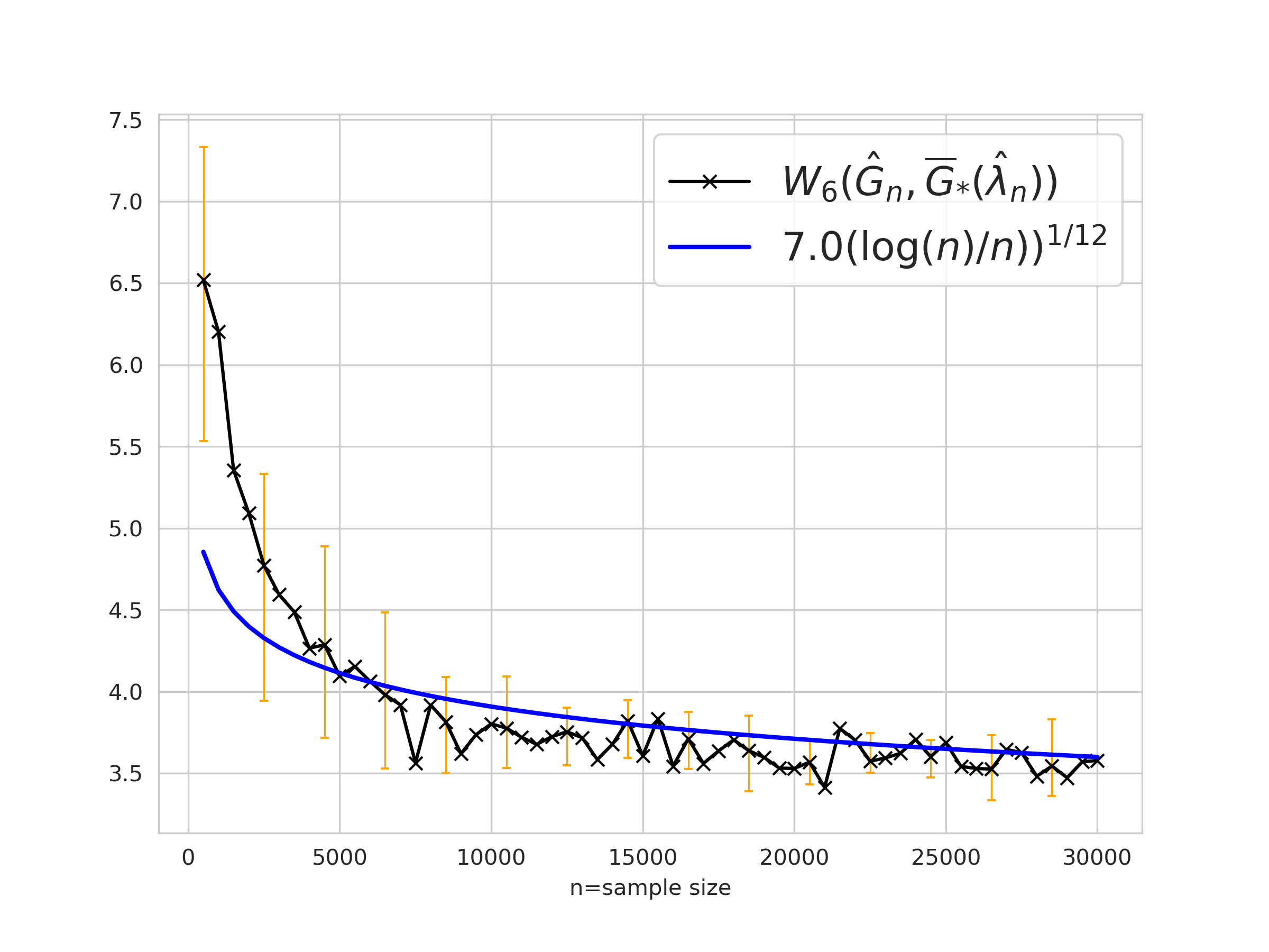
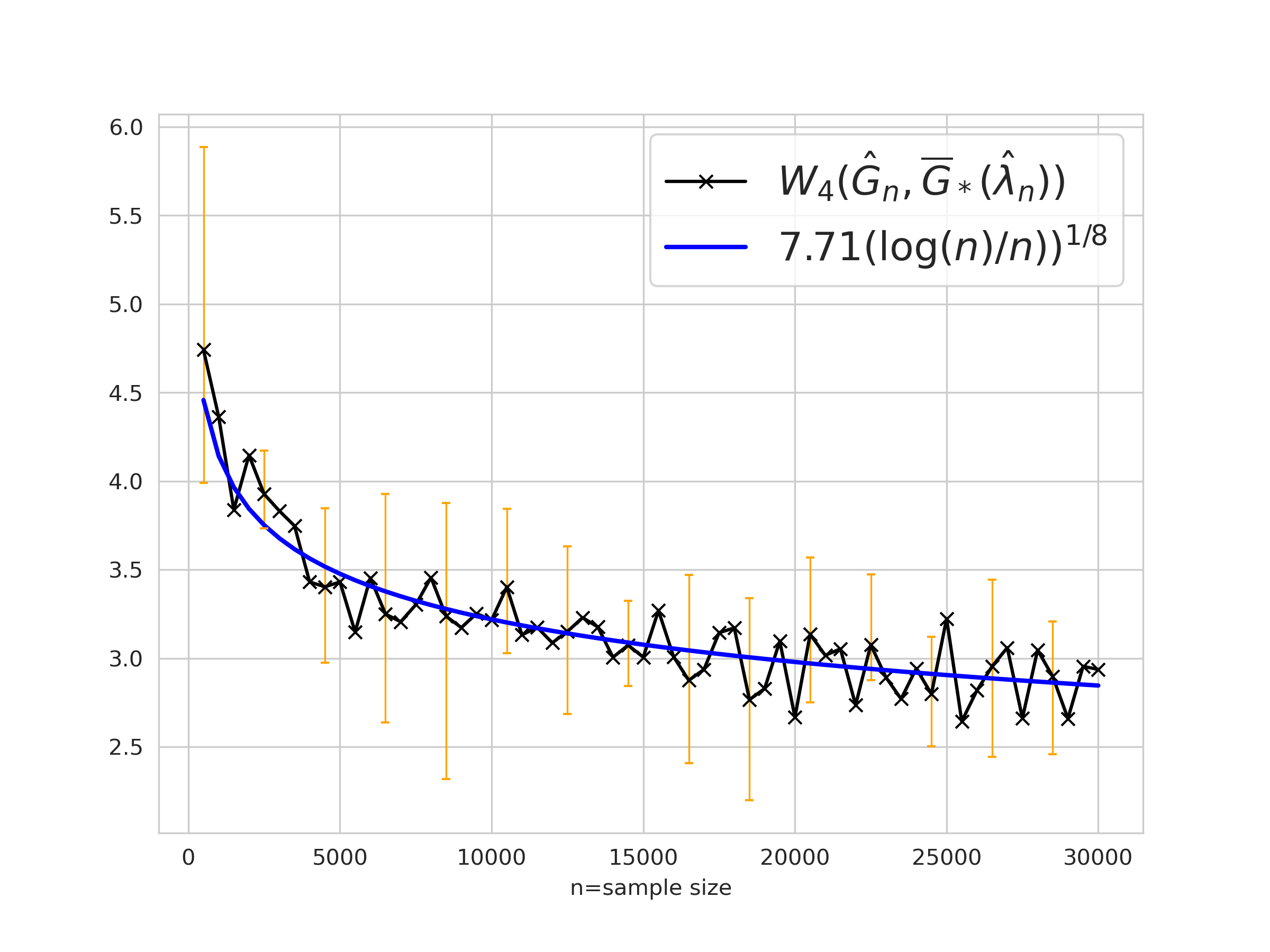
Partially distinguishable setting. Consider the partial distinguishable case as in Theorem A.3 with weakly identifiable ff, we will conduct an experiment to distinguish two regimes in part (b) and (c) of the theorem, which are λ>λ∗\lambda>\lambda^{*} and λ≤λ∗\lambda\leq\lambda^{*}. We simulate nn data from the true data generating model (1), where p10=0.4,p20=0.6p_{1}^{0}=0.4,p_{2}^{0}=0.6, p1∗=1,λ∗=0.3p_{1}^{*}=1,\lambda^{*}=0.3, μ10=μ1∗=(−2,3),Σ10=Σ1∗=(3−1−12)\mu_{1}^{0}=\mu_{1}^{*}=(-2,3),\Sigma_{1}^{0}=\Sigma_{1}^{*}=\begin{pmatrix}3&-1\\ -1&2\end{pmatrix}, μ20=(1,−4),Σ20=(1004)\mu_{2}^{0}=(1,-4),\Sigma_{2}^{0}=\begin{pmatrix}1&0\\ 0&4\end{pmatrix}. In this case, k∗=1,k0=2,k¯=1k_{*}=1,k_{0}=2,\bar{k}=1, k∗+k0−k¯=2k_{*}+k_{0}-\overline{k}=2 and we will fit the data with model pλ​Gp_{\lambda G}, where GG has 3 atoms. The MLE (λ^n,G^n)(\hat{\lambda}_{n},\hat{G}_{n}) is found by the EM algorithm. In the regime λ^n<λ∗\hat{\lambda}_{n}<\lambda^{*}, we see that λ^n→λ∗\hat{\lambda}_{n}\to\lambda^{*} in the parametric rate and the convergence of G^n\hat{G}_{n} to G∗G_{*} is of order (log⁡(n)/n)2​r¯​(K−k∗)=(log⁡(n)/n)12(\log(n)/n)^{2\overline{r}(K-k_{*})}=(\log(n)/n)^{12} (Fig. 2). When λ^n>λ∗\hat{\lambda}_{n}>\lambda^{*}, because of the indistinguishability of the model, we do not expect λ^n→λ∗\hat{\lambda}_{n}\to\lambda^{*} but the Wasserstein distance between G^n\hat{G}_{n} and G¯∗​(λ^n)\overline{G}_{*}(\hat{\lambda}_{n}) converges to 0 with the rate (log⁡(n)/n)2​r¯​(2)=(log⁡(n)/n)1/8(\log(n)/n)^{2\overline{r}(2)}=(\log(n)/n)^{1/8}. The simulation study matches with this result, where λ^n\hat{\lambda}_{n} converges to some number greater than λ∗\lambda^{*}, and the rate that W4​(G,G¯∗​(λ^n))W_{4}(G,\overline{G}_{*}(\hat{\lambda}_{n})) converges to 0 is of order (log⁡(n)/n)1/8(\log(n)/n)^{1/8} (Fig. 3).

(a) Convergence rates of W6​(G^n,G∗)W_{6}(\hat{G}_{n},G_{*})

(a) *
Refer to caption

(b) Convergence rates of |λ^n−λ∗||\hat{\lambda}_{n}-\lambda^{*}|

(b) *
Refer to caption
Figure 2: Parameter learning rates in regime λ≤λ∗\lambda\leq\lambda^{*}.

(a) Convergence rates of W4​(G^n,G∗)W_{4}(\hat{G}_{n},G_{*})

(a) *
Refer to caption

(b) Limit of λ^n\hat{\lambda}_{n}

(b) *
Refer to caption
Figure 3: Parameter learning rates in regime λ>λ∗\lambda>\lambda^{*}.

Appendix C Proofs of Section 2

C.1 Proof of Theorem 2.4

(a) We first prove that h0h_{0} is distinguishable with (f,k)(f,k) up to first order with any kk and ff being location-scale Gaussian family, i.e., if there exists λ,αj∈ℝ,βj∈ℝd,\lambda,\alpha_{j}\in\mathbb{R},\beta_{j}\in\mathbb{R}^{d}, symmetric matrices γi∈ℝd×d\gamma_{i}\in\mathbb{R}^{d\times d}, θj∈ℝd\theta_{j}\in\mathbb{R}^{d}, and positive definite symmetric Σj∈ℝd×d\Sigma_{j}\in\mathbb{R}^{d\times d} for j=1,…,kj=1,\dots,k such that

λ​h0​(x)+∑j=1kαj​f​(x|θj,Σj)+∑j=1kβjT​∂f∂θ​(x|θj,Σj)+tr⁡(∂f∂Σ​(x|θj,Σj)T​γj)=0,\lambda h_{0}(x)+\sum_{j=1}^{k}\alpha_{j}f(x|\theta_{j},\Sigma_{j})+\sum_{j=1}^{k}\beta_{j}^{T}\dfrac{\partial f}{\partial\theta}(x|\theta_{j},\Sigma_{j})+\operatorname{tr}\left(\dfrac{\partial f}{\partial\Sigma}(x|\theta_{j},\Sigma_{j})^{T}\gamma_{j}\right)=0,

then λ=αj=βj=γj=0\lambda=\alpha_{j}=\beta_{j}=\gamma_{j}=0 for all j=1,…,kj=1,\dots,k, where f⁡(x|θ,Σ)f(x|\theta,\Sigma) is the density evaluated at xx of Gaussian distribution with mean θ\theta and covariance Σ\Sigma and (θj,Σj)j=1k(\theta_{j},\Sigma_{j})_{j=1}^{k} are pairwise different. Suppose there exists such (λ,αj,βj,γj)j=1k(\lambda,\alpha_{j},\beta_{j},\gamma_{j})_{j=1}^{k}. We borrow a technique from [17, 28], where we find a one-dimensional space to project x∈ℝdx\in\mathbb{R}^{d} onto and work with the order of means and variances in that space to show that the solution must be trivial. Calculating the first derivatives of ff gives

λ​h0​(x)+∑j=1k(αj′+(βj′)T​(x−θj)+(x−θj)T​γj−1​(x−θj))​e−12​(x−θj)T​Σj−1​(x−θj)=0,\lambda h_{0}(x)+\sum_{j=1}^{k}\left(\alpha_{j}^{\prime}+(\beta_{j}^{\prime})^{T}(x-\theta_{j})+(x-\theta_{j})^{T}\gamma_{j}^{-1}(x-\theta_{j})\right)e^{-\dfrac{1}{2}(x-\theta_{j})^{T}\Sigma_{j}^{-1}(x-\theta_{j})}=0, (16)

where

αj′=2​αj−tr⁡(Σj−1​γj)2​πd/2​|Σj|1/2,βj′=2πd/2​|Σj|1/2​Σj−1​βj,γj′=1πd/2​|Σj|1/2​Σj−1​γj​Σj−1,\alpha_{j}^{\prime}=\dfrac{2\alpha_{j}-\operatorname{tr}(\Sigma_{j}^{-1}\gamma_{j})}{2\pi^{d/2}|\Sigma_{j}|^{1/2}},\quad\beta_{j}^{\prime}=\dfrac{2}{\pi^{d/2}|\Sigma_{j}|^{1/2}}\Sigma_{j}^{-1}\beta_{j},\quad\gamma_{j}^{\prime}=\dfrac{1}{\pi^{d/2}|\Sigma_{j}|^{1/2}}\Sigma_{j}^{-1}\gamma_{j}\Sigma_{j}^{-1},

for all j=1,…,kj=1,\dots,k. If all the covariance matrices are equal, i.e., Σ1=⋯=Σk\Sigma_{1}=\dots=\Sigma_{k}, then (θj)j=1k(\theta_{j})_{j=1}^{k} are pairwise different. Denote by δi​j=θi−θj\delta_{ij}=\theta_{i}-\theta_{j}, then for any x′∉∪1≤i≤j≤k{u∈ℝd:δi​jTu=0}x^{\prime}\not\in\cup_{1\leq i\leq j\leq k}\{u\in\mathbb{R}^{d}:\delta_{ij}^{T}u=0\}, we have (x′)T​θ1,…,(x′)T​θk(x^{\prime})^{T}\theta_{1},\dots,(x^{\prime})^{T}\theta_{k} are distinct. Otherwise, if (without loss of generality) there are Σ1,…,Σm\Sigma_{1},\dots,\Sigma_{m} different matrices among Σ1,…,Σk\Sigma_{1},\dots,\Sigma_{k}, then for every x′∉∪1≤i≤j≤m{u∈ℝd:uT(Σi−Σj)u=0}x^{\prime}\not\in\cup_{1\leq i\leq j\leq m}\{u\in\mathbb{R}^{d}:u^{T}(\Sigma_{i}-\Sigma_{j})u=0\}, we have (x′)T​Σ1​(x′),…,(x′)T​Σm​(x′)(x^{\prime})^{T}\Sigma_{1}(x^{\prime}),\dots,(x^{\prime})^{T}\Sigma_{m}(x^{\prime}) are distinct. In both cases, we find a finite collection of hyperplanes and cones such that for every x′x^{\prime} not belongs to any set of this collection, we have ((x′)T​θ1,(x′)T​Σ1​(x′)),…,((x′)T​θk,(x′)T​Σk​(x′))((x^{\prime})^{T}\theta_{1},(x^{\prime})^{T}\Sigma_{1}(x^{\prime})),\dots,((x^{\prime})^{T}\theta_{k},(x^{\prime})^{T}\Sigma_{k}(x^{\prime})) are pairwise different. Note that because the union of these collection of (d−1)(d-1) dimensional manifolds can not be ℝd\mathbb{R}^{d}, such a non-zero x′x^{\prime} exists. Now we only consider xx belongs to the one-dimensional linear space spanned by this x′x^{\prime}, i.e., x=y⁡(x′)x=y(x^{\prime}), where y∈ℝy\in\mathbb{R}. Denote by

aj=(x′)T​γj′​x′,bj=[(βj′)T−2​θjT​γj′]​x′,cj=θjT​γj′​γj−(βj′)T​θj,a_{j}=(x^{\prime})^{T}\gamma_{j}^{\prime}x^{\prime},\,\,b_{j}=[(\beta_{j}^{\prime})^{T}-2\theta_{j}^{T}\gamma_{j}^{\prime}]x^{\prime},\,\,c_{j}=\theta_{j}^{T}\gamma_{j}^{\prime}\gamma_{j}-(\beta_{j}^{\prime})^{T}\theta_{j},
dj=(x′)T​Σj−1​x′,ej=(x′)T​Σj−1​θj′,fi=θjT​Σj−1​θj,d_{j}=(x^{\prime})^{T}\Sigma_{j}^{-1}x^{\prime},\,\,e_{j}=(x^{\prime})^{T}\Sigma_{j}^{-1}\theta_{j}^{\prime},\,\,f_{i}=\theta_{j}^{T}\Sigma_{j}^{-1}\theta_{j},

for j=1,…,kj=1,\dots,k, we proved that ((dj,ej))j=1k((d_{j},e_{j}))_{j=1}^{k} are distinct. Equation (16) implies that

λ​h0​(y​x′)+∑j=1k(αj′+aj​y2+bj​y+cj)​exp⁡(dj​y2+ej​y+fj)=0.\lambda h_{0}(yx^{\prime})+\sum_{j=1}^{k}(\alpha_{j}^{\prime}+a_{j}y^{2}+b_{j}y+c_{j})\exp(d_{j}y^{2}+e_{j}y+f_{j})=0. (17)
Case 1.

If −log⁡h0​(x)≳‖x‖2β1-\log h_{0}(x)\gtrsim\left\|x\right\|_{2}^{\beta_{1}} for some β1>2\beta_{1}>2 and for all ‖x‖2>x0\left\|x\right\|_{2}>x_{0}, we have h0​(x)≲exp−‖x‖2β1h_{0}(x)\lesssim\exp^{-\left\|x\right\|_{2}^{\beta_{1}}}. Choose di1=max1≤i≤k⁡dkd_{i_{1}}=\max_{1\leq i\leq k}d_{k} and ei2=max⁡{ej:dj=dj1}e_{i_{2}}=\max\{e_{j}:d_{j}=d_{j_{1}}\}. Because h0h_{0} has a lighter tail than Gaussian and

dj​y2+ej​y+fj<di2​y2+ei2​y+fi2,∀j≠i2,d_{j}y^{2}+e_{j}y+f_{j}<d_{i_{2}}y^{2}+e_{i_{2}}y+f_{i_{2}},\quad\forall j\neq i_{2},

for all yy large enough, divide both sides of (17) by exp⁡(di2​y2+ei2​y+fi2)\exp(d_{i_{2}}y^{2}+e_{i_{2}}y+f_{i_{2}}) and let y→∞y\to\infty, we have ai2=bi2=0a_{i_{2}}=b_{i_{2}}=0. It implies that (x′)T​γi2′​x′=[(βi2′)T−2​θi2T​γi2′]​x′=0(x^{\prime})^{T}\gamma_{i_{2}}^{\prime}x^{\prime}=[(\beta_{i_{2}}^{\prime})^{T}-2\theta_{i_{2}}^{T}\gamma_{i_{2}}^{\prime}]x^{\prime}=0. If γi2′≠0\gamma_{i_{2}}^{\prime}\neq 0 then we can further choose x′x^{\prime} outside a cone such that (x′)T​γi2′​x′≠0(x^{\prime})^{T}\gamma_{i_{2}}^{\prime}x^{\prime}\neq 0. Hence, γi2=0\gamma_{i_{2}}=0, which implies (βi2′)T​(x′)=0(\beta_{i_{2}}^{\prime})^{T}(x^{\prime})=0. If βi2≠0\beta_{i_{2}}\neq 0 then we can further choose x′x^{\prime} outside a hyperplane such that (βi2′)T​(x′)≠0(\beta_{i_{2}}^{\prime})^{T}(x^{\prime})\neq 0. Hence, in any case, we can argue so that βi2′=θi2′=0\beta^{\prime}_{i_{2}}=\theta^{\prime}_{i_{2}}=0. Put it back to (17), we also have αi2′=0\alpha^{\prime}_{i_{2}}=0. Therefore, αi2=βi2=γi2=0\alpha_{i_{2}}=\beta_{i_{2}}=\gamma_{i_{2}}=0. Repeat the same argument, notice that the tail of h0h_{0} is lighter than any Gaussian distribution, we have αj=βj=γj=0\alpha_{j}=\beta_{j}=\gamma_{j}=0 for all j=1,…,kj=1,\dots,k. It finally leads to λ=0\lambda=0. Hence, we have the distinguishability of h0h_{0} with family of location-scale Gaussians up to first order.

Case 2.

If −log⁡h0​(x)≲‖x‖2β2-\log h_{0}(x)\lesssim\left\|x\right\|_{2}^{\beta_{2}} for some β2<2\beta_{2}<2 and for all ‖x‖2>x0\left\|x\right\|_{2}>x_{0}. We have p⁡(x|θj,Σj)/h0​(x)→0p(x|\theta_{j},\Sigma_{j})/h_{0}(x)\to 0 as x→∞x\to\infty for all j=1,…,kj=1,\dots,k. Therefore, dividing both sides of (16) by h0​(x)h_{0}(x) and let x→∞x\to\infty by some direction, we have λ=0\lambda=0. Now proceed to argue similar to Case 1, we also have the distinguishability of h0h_{0} with family of location-scale Gaussians up to first order.

Now we proceed to prove that h0h_{0} is distinguishable with (f,k)(f,k) up to the any order, for ff being family of location Gaussian and any k>0k>0. Arguing similar to above, we only need to work on one-dimensional space. Suppose that there exists λ,(ci,j)i=1,…,k,j=1,…,r\lambda,(c_{i,j})_{i=1,\dots,k,j=1,\dots,r} such that

λ​h0​(x)+∑i=1k∑j=0rci,j​∂jf∂θj​(x|θi,vi)=0,\lambda h_{0}(x)+\sum_{i=1}^{k}\sum_{j=0}^{r}c_{i,j}\dfrac{\partial^{j}f}{\partial\theta^{j}}(x|\theta_{i},v_{i})=0, (18)

where f(⋅|θ,v)f(\cdot|\theta,v) is the density function of normal distribution with mean θ\theta and variance vv, and (θ1,v1),…,(θk,vk)(\theta_{1},v_{1}),\dots,(\theta_{k},v_{k}) are distinct. We need to prove that λ=ci,j=0\lambda=c_{i,j}=0 for all i=1,…,k,j=1,…,ri=1,\dots,k,j=1,\dots,r. Calculating the partial derivatives of ff, we have

λ​h0​(x)+∑i=1k(∑j=0rγi,j​(x−θi)j)​exp⁡(−(x−θi)22​vi)=0,\lambda h_{0}(x)+\sum_{i=1}^{k}\left(\sum_{j=0}^{r}\gamma_{i,j}(x-\theta_{i})^{j}\right)\exp\left(-\dfrac{(x-\theta_{i})^{2}}{2v_{i}}\right)=0, (19)

such that γi,j\gamma_{i,j} for odd j are linear combination of (ci,l)(c_{i,l}) with odd l≤jl\leq j, γi,j\gamma_{i,j} for even j are linear combination of (ci,l)(c_{i,l}) with even l≤jl\leq j, and one can prove (for example, by induction) that γi,j=0​∀j\gamma_{i,j}=0\forall j is equivalent to ci,j=0​∀jc_{i,j}=0\forall j. Now we can argue similar to Case 1 and Case 2 above to get the contradiction, with the notice that polynomials grow slower than exponential functions.

(b) Let TT be a piecewise linear function with a positive finite number of breakpoints and h0h_{0} is the density function of N⁡(0,Id)N(0,I_{d}) being pushforwarded by TT. Argue similar to above, we only need to prove the result in one-dimensional case. In order to prove the distinguishable of h0h_{0} with mixtures of location Gaussians family or mixtures of location-scale Gaussians family, it all boils down to prove that if there exists λ∈ℝ\lambda\in\mathbb{R} and polynomials Q1​(x),Q2​(x),…,Qk​(x)Q_{1}(x),Q_{2}(x),\dots,Q_{k}(x) such that

λ​h0​(x)+∑i=1kQi​(x)​f​(x|θi,vi2)=0,\lambda h_{0}(x)+\sum_{i=1}^{k}Q_{i}(x)f(x|\theta_{i},v_{i}^{2})=0, (20)

where (θ1,v12),…,(θk,vk2)(\theta_{1},v_{1}^{2}),\dots,(\theta_{k},v_{k}^{2}) are distinct, then λ=Q1​(x)=⋯=Qk​(x)=0\lambda=Q_{1}(x)=\dots=Q_{k}(x)=0. We will prove this by induction in kk. Consider the case k=1k=1, we have

λ​h0​(x)+Q1​(x)​f​(x|θ1,v12)=0.\lambda h_{0}(x)+Q_{1}(x)f(x|\theta_{1},v_{1}^{2})=0. (21)

Because TT has finite number of break points, there exists some x0x_{0} large enough so that for all x>x0x>x_{0}, TT is a linear one-to-one function between [x0,∞)[x_{0},\infty) and its image. Denote by T⁡(x)=a​x+bT(x)=ax+b when x>x0x>x_{0}. We can argue that a≠0a\neq 0, because otherwise the distribution of h0h_{0} will has an atom, which directly leads to distinguishability between h0h_{0} and mixtures of Gaussians. Then, h0​(x)=f⁡(x|b,a2)h_{0}(x)=f(x|b,a^{2}) and we have

λ​f​(x|b,a2)+Q1​(x)​f​(x|θ1,v12)=0.\lambda f(x|b,a^{2})+Q_{1}(x)f(x|\theta_{1},v_{1}^{2})=0.

Argue similar to part (a), if (b,a2)≠(θ1,v12)(b,a^{2})\neq(\theta_{1},v_{1}^{2}), we have λ=Q1​(x)=0\lambda=Q_{1}(x)=0, which implies the distinguishability. Otherwise, we have b=θ1,a2=v12b=\theta_{1},a^{2}=v_{1}^{2}, and Q1​(x)=−λQ_{1}(x)=-\lambda for all x∈ℝx\in\mathbb{R}. We can rewrite (21) as

h0​(x)−f⁡(x|θ1,v12)=0.h_{0}(x)-f(x|\theta_{1},v_{1}^{2})=0.

Because h0h_{0} is N⁡(0,1)N(0,1) being pushforwarded by a piecewise linear function, we can write ℝ\mathbb{R} as a partition (−∞,c1],(c1,c2],…,[cm,∞)(-\infty,c_{1}],(c_{1},c_{2}],\dots,[c_{m},\infty) such that each semi-open interval is image of some linear functions of TT. Consider a semi-open interval (ci,ci+i](c_{i},c_{i+i}] being image of Tj​(z)=aj​z+bjT_{j}(z)=a_{j}z+b_{j} for j=1,…,hj=1,\dots,h, by the change of variable formula for many-to-one map, we have

0=h0​(x)−f⁡(x|θ1,v12)=∑j=1hf⁡(x|bj,aj2)−f⁡(x|θ1,v12),0=h_{0}(x)-f(x|\theta_{1},v_{1}^{2})=\sum_{j=1}^{h}f(x|b_{j},a_{j}^{2})-f(x|\theta_{1},v_{1}^{2}), (22)

for all x∈(ci,ci+i]x\in(c_{i},c_{i+i}]. Applying Lemma C.1, we have equation (22) is true for all x∈ℝx\in\mathbb{R}. Hence, by integrating both side, we get h=1h=1, and then b1=θ1,a12=v12b_{1}=\theta_{1},a_{1}^{2}=v_{1}^{2}. Because this is true for all semi-open intervals (ci,ci+i](c_{i},c_{i+i}], we have T⁡(x)=a1​x+b1T(x)=a_{1}x+b_{1} for all x∈ℝx\in\mathbb{R}, which is contradict to our assumption that TT is non-linear.

Suppose that our inductive hypothesis is correct for k=nk=n, now we proceed to prove it is true for k=n+1k=n+1. If there exists λ∈ℝ\lambda\in\mathbb{R} and polynomials Q1​(x),Q2​(x),…,Qn+1​(x)Q_{1}(x),Q_{2}(x),\dots,Q_{n+1}(x) such that

λ​h0​(x)+∑i=1n+1Qi​(x)​f​(x|θi,vi2)=0,\lambda h_{0}(x)+\sum_{i=1}^{n+1}Q_{i}(x)f(x|\theta_{i},v_{i}^{2})=0, (23)

where (θ1,v1),…,(θn+1,vn+12)(\theta_{1},v_{1}),\dots,(\theta_{n+1},v_{n+1}^{2}) are distinct. Without loss of generality, assume that v12=max1≤i≤n+1⁡vk2v^{2}_{1}=\max_{1\leq i\leq n+1}v^{2}_{k} and θ1=max⁡{θj:vj2=v12}\theta_{1}=\max\{\theta_{j}:v_{j}^{2}=v_{1}^{2}\}. Because TT has finite number of break points, there exists some x0x_{0} large enough so that for all x>x0x>x_{0}, TT is a linear one-to-one function between [x0,∞)[x_{0},\infty) and its image. Denote by T⁡(x)=a​x+bT(x)=ax+b when x>x0x>x_{0}. We have

λ​f​(x|b,a2)+∑i=1n+1Qi​(x)​f​(x|θi,vi2)=0,∀x>x0.\lambda f(x|b,a^{2})+\sum_{i=1}^{n+1}Q_{i}(x)f(x|\theta_{i},v_{i}^{2})=0,\quad\forall\,x>x_{0}. (24)

If a2>v12a^{2}>v_{1}^{2} or a2=v12,b>θ1a^{2}=v_{1}^{2},b>\theta_{1}, divide both sides of equation (24) by exp⁡((x−b)/2​a2)\exp((x-b)/2a^{2}) and let x→∞x\to\infty, we have λ=0\lambda=0 and the conclusion follows from the identifiability of Gaussians family.

If v12>a2v_{1}^{2}>a^{2} or v12=a2,θ1>bv_{1}^{2}=a^{2},\theta_{1}>b, divide both sides of equation (24) by exp⁡((x−θ1)/2​v12)\exp((x-\theta_{1})/2v_{1}^{2}) and let x→∞x\to\infty, we have Q1​(x)=0Q_{1}(x)=0. The problem is back to the case k=nk=n and is proved using the inductive hypothesis.

If a2=v12,b=θ1a^{2}=v_{1}^{2},b=\theta_{1}, divide both sides of equation (24) by exp⁡((x−b)/2​a2)\exp((x-b)/2a^{2}) and let x→∞x\to\infty, we have Q1​(x)=−λQ_{1}(x)=-\lambda for all x∈ℝx\in\mathbb{R}. Hence for xx large enough,

∑i=2n+1Qi​(x)​f​(x|θi,vi2)=0,\sum_{i=2}^{n+1}Q_{i}(x)f(x|\theta_{i},v_{i}^{2})=0,

which implies Q2​(x)=⋯=Qn+1​(x)=0Q_{2}(x)=\dots=Q_{n+1}(x)=0. The problem is back to the case k=1k=1 and is proved using the inductive hypothesis.

The following lemma presents the local identifiability of location-scale Gaussians mixtures.

Lemma C.1.

Denote by f(⋅|θ,σ2)f(\cdot|\theta,\sigma^{2}) the density function of Gaussian distribution with mean θ\theta and variance σ2\sigma^{2}. For all a<ba<b and pairs {(θi,σi2)}i=1k\{(\theta_{i},\sigma_{i}^{2})\}_{i=1}^{k}, if there exists α1,α2,…,αn∈ℝ\alpha_{1},\alpha_{2},\dots,\alpha_{n}\in\mathbb{R} such that

α1​f​(x|θ1,σ12)+⋯+αk​f​(x|θk,σk2)=0\alpha_{1}f(x|\theta_{1},\sigma_{1}^{2})+\dots+\alpha_{k}f(x|\theta_{k},\sigma_{k}^{2})=0

for all x∈[a,b]x\in[a,b], then

α1​f​(x|θ1,σ12)+⋯+αk​f​(x|θk,σk2)=0,\alpha_{1}f(x|\theta_{1},\sigma_{1}^{2})+\dots+\alpha_{k}f(x|\theta_{k},\sigma_{k}^{2})=0, (25)

for all x∈ℝx\in\mathbb{R}.

Proof.

Step 1. (Centralize and normalize coefficients). Suppose that there exists α1,α2,…,αn∈ℝ\alpha_{1},\alpha_{2},\dots,\alpha_{n}\in\mathbb{R} such that

α1​f​(x|θ1,σ12)+⋯+αk​f​(x|θk,σk2)=0\alpha_{1}f(x|\theta_{1},\sigma_{1}^{2})+\dots+\alpha_{k}f(x|\theta_{k},\sigma_{k}^{2})=0

for all x∈[a,b]x\in[a,b]. Denote by θi′=θi−a+b2\theta^{\prime}_{i}=\theta_{i}-\dfrac{a+b}{2} for all i=1,…,ki=1,\dots,k, then

α1​12​π​σ1​exp⁡(−(x−θ1′)22​σ12)+⋯+αk​12​π​σk​exp⁡(−(x−θk′)22​σk2)=0,\alpha_{1}\dfrac{1}{\sqrt{2\pi}\sigma_{1}}\exp\left(-\dfrac{(x-\theta_{1}^{\prime})^{2}}{2\sigma_{1}^{2}}\right)+\dots+\alpha_{k}\dfrac{1}{\sqrt{2\pi}\sigma_{k}}\exp\left(-\dfrac{(x-\theta_{k}^{\prime})^{2}}{2\sigma_{k}^{2}}\right)=0, (26)

for all x∈[−b−a2,b−a2]x\in[-\frac{b-a}{2},\frac{b-a}{2}]. Denote by σi1=min⁡{α1,…,αk}\sigma_{i_{1}}=\min\{\alpha_{1},\dots,\alpha_{k}\}. Multiple both sides of (26) by exp⁡(−x2σi12)\exp(-\frac{x^{2}}{\sigma_{i_{1}}^{2}}), and denote by si2=1σi12−12​σi2,mi=θi′/σi2,βi=12​π​σiexp(−(θi′)2/2σi2)s_{i}^{2}=\frac{1}{\sigma_{i_{1}}^{2}}-\frac{1}{2\sigma_{i}^{2}},m_{i}=\theta_{i}^{\prime}/\sigma_{i}^{2},\beta_{i}=\dfrac{1}{\sqrt{2\pi}\sigma_{i}}\exp(-(\theta_{i}^{\prime})^{2}/2\sigma_{i}^{2}) for all i=1,…,ki=1,\dots,k, we have

β1​exp⁡(s12​x2+m1​x)+⋯+βk​exp⁡(sk2​x2+mk​x)=0,\beta_{1}\exp\left(s_{1}^{2}x^{2}+m_{1}x\right)+\dots+\beta_{k}\exp\left(s_{k}^{2}x^{2}+m_{k}x\right)=0, (27)

for all x∈[−b−a2,b−a2]x\in[-\frac{b-a}{2},\frac{b-a}{2}].

Step 2. (Use properties of Laplace transformation). The left-hand side of equation (27) is the Laplace transformation of ∑i=1kβi​f​(x|mi,si2)\sum_{i=1}^{k}\beta_{i}f(x|m_{i},s_{i}^{2}) and is identical to 0 in an open set around 0. Hence

∑i=1kβi​f​(x|mi,si2)=0,\sum_{i=1}^{k}\beta_{i}f(x|m_{i},s_{i}^{2})=0,

for all x∈ℝx\in\mathbb{R}. It implies that

β1​exp⁡(s12​x2+m1​x)+⋯+βk​exp⁡(sk2​x2+mk​x)=0,\beta_{1}\exp\left(s_{1}^{2}x^{2}+m_{1}x\right)+\dots+\beta_{k}\exp\left(s_{k}^{2}x^{2}+m_{k}x\right)=0,

for all x∈ℝx\in\mathbb{R}, which is equivalent to equation (25). ∎

C.2 Proof of Proposition 2.5

If kσk_{\sigma} is the Gaussian kernel with m>Km>K, then we get the conclusions as direct consequences of Example 2.3(a). If kσk_{\sigma} is the multivariate Student kernel, then h0h_{0} has a tail heavier than Gaussian tail, so that we get the conclusions as consequences of Proposition 2.4(a).

C.3 Proof of Proposition 2.6

Because TT has a finite and postive number of layers, it is a piecewise linear and non-linear function. So the conclusions are direct consequences of Proposition 2.4(b).

C.4 Proof of Theorem 3.1

This result can be obtained by modifying the proof of Theorem 7.4 in [26]. Recall that we defined the function class

𝒫¯k1/2(Θ,ϵ)={p¯λ​G1/2:G∈𝒪k(Θ),h(p¯λ​G,pλ∗​G∗)≤ϵ},\overline{\mathcal{P}}^{1/2}_{k}(\Theta,\epsilon)=\left\{\bar{p}_{\lambda G}^{1/2}:G\in\mathcal{O}_{k}(\Theta),~h(\bar{p}_{\lambda G},p_{\lambda^{*}G_{*}})\leq\epsilon\right\}, (28)

where for any G∈𝒪K​(Θ)G\in\mathcal{O}_{K}(\Theta), we write p¯λ​G=(pλ​G+pλ∗​G∗)/2\bar{p}_{\lambda G}=(p_{\lambda G}+p_{\lambda^{*}G_{*}})/2, and measure the complexity of this class through the bracketing entropy integral

𝒥B​(ϵ,𝒫¯k1/2​(Θ,ϵ),ν)=∫ϵ2/213ϵlog⁡NB​(u,𝒫¯k1/2​(Θ,u),ν)​𝑑u∨ϵ,\mathcal{J}_{B}(\epsilon,\overline{\mathcal{P}}^{1/2}_{k}(\Theta,\epsilon),\nu)=\int_{\epsilon^{2}/2^{13}}^{\epsilon}\sqrt{\log N_{B}(u,\overline{\mathcal{P}}_{k}^{1/2}(\Theta,u),\nu)}du\vee\epsilon,

where NB​(ϵ,X,η)N_{B}(\epsilon,X,\eta) denotes the ϵ\epsilon-bracketing number of a metric space (X,η)(X,\eta) and ν\nu is the Lebesgue measure. We denote by Pλ​GP_{\lambda G} the distribution corresponding to the density pλ​Gp_{\lambda G}. The technique to prove this theorem is to bound the convergence rate by the increments of an empirical processes:

νn​(λ​G)=n​∫{pλ∗​G∗}>012​log⁡p¯λ​Gpλ∗​G∗​d​(Pn−Pλ∗​G∗),\nu_{n}(\lambda G)=\sqrt{n}\int_{\{p_{\lambda^{*}G_{*}}\}>0}\dfrac{1}{2}\log\dfrac{\overline{p}_{\lambda G}}{p_{\lambda^{*}G_{*}}}d(P_{n}-P_{\lambda^{*}G_{*}}),

where Pn=1n​∑i=1nδXiP_{n}=\frac{1}{n}\sum_{i=1}^{n}\delta_{X_{i}} is the empirical measure (X1,…,Xn​∼i​i​d​pλ∗​G∗X_{1},\dots,X_{n}\overset{iid}{\sim}p_{\lambda^{*}G_{*}}). We first recall Theorem 5.11 in [26] with the notations adapted from our setting:

Theorem C.2.

Let R>0R>0, k≥1k\geq 1, and 𝒢\mathcal{G} be a subset of 𝒪k​(Θ)\mathcal{O}_{k}(\Theta), which contains G∗G_{*}. Given C1<∞C_{1}<\infty, for all CC sufficiently large, and for n∈ℕn\in\mathbb{N} and t>0t>0 satisfying

t≤n​((8​R)∧(C1​R2)),t\leq\sqrt{n}((8R)\wedge(C_{1}R^{2})), (29)

and

t≥C2​(C1+1)​(R∨∫t/(26​n)RHB1/2​(u2,𝒫¯k1/2​(Θ,R),ν)​𝑑u),t\geq C^{2}(C_{1}+1)\left(R\vee\int_{t/(2^{6}\sqrt{n})}^{R}H_{B}^{1/2}\left(\frac{u}{\sqrt{2}},\overline{\mathcal{P}}_{k}^{1/2}(\Theta,R),\nu\right)du\right), (30)

we have

ℙλ∗​G∗​(supG∈𝒢,h⁡(p¯λ​G,pλ∗​G∗)≤R|νn​(λ​G)|≥t)≤C​exp⁡(−t2C2​(C1+1)​R2).\mathbb{P}_{\lambda^{*}G_{*}}\left(\sup_{G\in\mathcal{G},h(\overline{p}_{\lambda G},p_{\lambda^{*}G_{*}})\leq R}|\nu_{n}(\lambda G)|\geq t\right)\leq C\exp\left(-\dfrac{t^{2}}{C^{2}(C_{1}+1)R^{2}}\right). (31)

Now we proceed to prove Theorem 3.1, the proof is divided into three parts: Bounding the tail probability of h⁡(pλ^n​G^n,pλ∗​G∗)h(p_{\hat{\lambda}_{n}\hat{G}_{n}},p_{\lambda^{*}G_{*}}) by sums of empirical processes increments using chaining technique, bounding the empirical processes increments using Theorem C.2, and bounding the expectation of h⁡(pλ^n​G^n,pλ∗​G∗)h(p_{\hat{\lambda}_{n}\hat{G}_{n}},p_{\lambda^{*}G_{*}}) using its tail probability.

Step 1 (Bounding the tail probability h⁡(pλ^n​G^n,pλ∗​G∗)h(p_{\hat{\lambda}_{n}\hat{G}_{n}},p_{\lambda^{*}G_{*}}) by sums of empirical processes increments):

Firstly, by Lemma 4.1 and 4.2 of [26], we have

116​h2​(pλ^n​G^n,pλ∗​G∗)≤h2​(p¯λ^n​G^n,pλ∗​G∗)≤1n​νn​(λ^n​G^n).\dfrac{1}{16}h^{2}(p_{\hat{\lambda}_{n}\hat{G}_{n}},p_{\lambda^{*}G_{*}})\leq h^{2}(\overline{p}_{\hat{\lambda}_{n}\hat{G}_{n}},p_{\lambda^{*}G_{*}})\leq\dfrac{1}{\sqrt{n}}\nu_{n}(\hat{\lambda}_{n}\hat{G}_{n}).

Hence, for any δ>δn:=(log⁡n/n)1/2\delta>\delta_{n}:=(\log n/n)^{1/2}, we have

ℙλ∗​G∗​(h⁡(pλ^n​G^n,pλ∗​G∗)≥δ)\displaystyle\mathbb{P}_{\lambda^{*}G_{*}}(h(p_{\hat{\lambda}_{n}\hat{G}_{n}},p_{\lambda^{*}G_{*}})\geq\delta) ≤ℙλ∗​G∗​(νn​(λ^n​G^n)−n​h2​(p¯λ^n​G^n,pλ∗​G∗)≥0CLOSE,\displaystyle\leq\mathbb{P}_{\lambda^{*}G_{*}}\bigg(\nu_{n}(\hat{\lambda}_{n}\hat{G}_{n})-\sqrt{n}h^{2}(\overline{p}_{\hat{\lambda}_{n}\hat{G}_{n}},p_{\lambda^{*}G_{*}})\geq 0,
OPENh⁡(p¯λ^n​G^n,pλ∗​G∗)≥δ/4)\displaystyle\hskip 142.26378pth(\overline{p}_{\hat{\lambda}_{n}\hat{G}_{n}},p_{\lambda^{*}G_{*}})\geq\delta/4\bigg)
≤ℙλ∗​G∗(supλ,G:h⁡(p¯λ​G,pλ∗​G∗)≥δ/4[νn(λG)−nh2(p¯λ​G,pλ∗​G∗)]≥0)\displaystyle\leq\mathbb{P}_{\lambda^{*}G_{*}}\left(\sup_{\lambda,G:h(\overline{p}_{\lambda G},p_{\lambda^{*}G_{*}})\geq\delta/4}[\nu_{n}(\lambda G)-\sqrt{n}h^{2}(\overline{p}_{\lambda G},p_{\lambda^{*}G_{*}})]\geq 0\right)
≤∑s=0Sℙλ∗​G∗(supλ,G:2s​δ/4≤h⁡(p¯λ​G,pλ∗​G∗)≤2s+1​δ/4|νn(λG)|≥n22​s(δ/4)2)\displaystyle\leq\sum_{s=0}^{S}\mathbb{P}_{\lambda^{*}G_{*}}\left(\sup_{\lambda,G:2^{s}\delta/4\leq h(\overline{p}_{\lambda G},p_{\lambda^{*}G_{*}})\leq 2^{s+1}\delta/4}|\nu_{n}(\lambda G)|\geq\sqrt{n}2^{2s}(\delta/4)^{2}\right)
≤∑s=0Sℙλ∗​G∗(supλ,G:h⁡(p¯λ​G,pλ∗​G∗)≤2s+1​δ/4|νn(λG)|≥n22​s(δ/4)2),\displaystyle\leq\sum_{s=0}^{S}\mathbb{P}_{\lambda^{*}G_{*}}\left(\sup_{\lambda,G:h(\overline{p}_{\lambda G},p_{\lambda^{*}G_{*}})\leq 2^{s+1}\delta/4}|\nu_{n}(\lambda G)|\geq\sqrt{n}2^{2s}(\delta/4)^{2}\right),

where SS is a smallest number such that 2S​δ/4>12^{S}\delta/4>1, as h⁡(p¯λ​G,pλ∗​G∗)≤1h(\overline{p}_{\lambda G},p_{\lambda^{*}G_{*}})\leq 1. Now we will bound the each term above using Theorem C.2.

Step 2 (Bounding the empirical processes increments using Theorem C.2):

In Theorem C.2, choose R=2s+1​δ,C1=15R=2^{s+1}\delta,C_{1}=15 and t=n​22​s​(δ/4)2t=\sqrt{n}2^{2s}(\delta/4)^{2}, we can readily check that Condition (29) satisfies (because 2s−1​δ/4≤12^{s-1}\delta/4\leq 1 for all s=0,…,Ss=0,\dots,S). Condition (30) satisfies thanks to Assumption A3:

∫t/(26​n)RHB1/2​(u2,𝒫k1/2​(Θ,R),ν)​𝑑u∨2s+1​δ\displaystyle\int_{t/(2^{6}\sqrt{n})}^{R}H_{B}^{1/2}\left(\dfrac{u}{\sqrt{2}},\mathcal{P}_{k}^{1/2}(\Theta,R),\nu\right)du\vee 2^{s+1}\delta =2​∫R2/213R/2HB1/2​(u,𝒫k1/2​(Θ,R),ν)​𝑑u∨2s+1​δ\displaystyle=\sqrt{2}\int_{R^{2}/2^{13}}^{R/\sqrt{2}}H_{B}^{1/2}\left(u,\mathcal{P}_{k}^{1/2}(\Theta,R),\nu\right)du\vee 2^{s+1}\delta
≤2​𝒥B​(R,𝒫1/2​(Θ,R),ν)\displaystyle\leq 2\mathcal{J}_{B}(R,\mathcal{P}^{1/2}(\Theta,R),\nu)
≤2​J​n​22​s+1​δ2=26​J​t.\displaystyle\leq 2J\sqrt{n}2^{2s+1}\delta^{2}=2^{6}Jt.

So the conclusion of Theorem C.2 gives us

ℙλ∗​G∗​(h⁡(pλ^n​G^n,pλ∗​G∗)>δ)≤C​∑s=0∞exp⁡(22​s​n​δ2J2​214)≤c​exp⁡(n​δ2c2),\mathbb{P}_{\lambda^{*}G_{*}}(h(p_{\hat{\lambda}_{n}\hat{G}_{n}},p_{\lambda^{*}G_{*}})>\delta)\leq C\sum_{s=0}^{\infty}\exp\left(\dfrac{2^{2s}n\delta^{2}}{J^{2}2^{14}}\right)\leq c\exp\left(\dfrac{n\delta^{2}}{c^{2}}\right), (32)

where cc is a large constants that does not depend on λ∗,G∗\lambda^{*},G_{*}.

Step 3 (Implying the bound on supremum of expectation):

Thus, we have

𝔼​h​(pλ^n​G^n,pλ∗​G∗)=∫0∞ℙ⁡(h⁡(pλ^n​G^n,pλ∗​G∗)>δ)​𝑑δ≤δn+c​∫δn∞exp⁡(−n​δ2c2)≤c~​δn,\mathbb{E}h(p_{\hat{\lambda}_{n}\hat{G}_{n}},p_{\lambda^{*}G_{*}})=\int_{0}^{\infty}\mathbb{P}(h(p_{\hat{\lambda}_{n}\hat{G}_{n}},p_{\lambda^{*}G_{*}})>\delta)d\delta\leq\delta_{n}+c\int_{\delta_{n}}^{\infty}\exp\left(-\dfrac{n\delta^{2}}{c^{2}}\right)\leq\tilde{c}\delta_{n},

for some c~\tilde{c} does not depend on λ∗,G∗\lambda^{*},G_{*}. Hence, we finally proved that

supG∗∈𝒪k​(Θ),λ∗∈[0,1]𝔼λ∗,G∗​h​(pλ^n​G^n,pλ∗​G∗)≤C​log⁡n/n.\sup_{G_{*}\in\mathcal{O}_{k}(\Theta),\lambda^{*}\in[0,1]}\mathbb{E}_{\lambda^{*},G_{*}}h(p_{\widehat{\lambda}_{n}\widehat{G}_{n}},p_{\lambda^{*}G_{*}})\leq C\sqrt{\log n/n}.

As a consequence, we obtain the conclusion of the theorem.

Appendix D Proof of Section 3

D.1 Proof of Proposition 3.2

We first need to denote some notations that are required for the proof. Those notations are well-known in Empirical Processes field [26]. Denote by

𝒫k(Θ)={pλ​G:λ∈[0,1],G∈𝒪k(Θ)},\mathcal{P}_{k}(\Theta)=\{p_{\lambda G}:\lambda\in[0,1],G\in\mathcal{O}_{k}(\Theta)\},

and let N(ϵ,𝒫k(Θ),∥⋅∥∞)N(\epsilon,\mathcal{P}_{k}(\Theta),\|\cdot\|_{\infty}) be the ϵ−\epsilon-covering number of (𝒫k(Θ,∥⋅∥∞)(\mathcal{P}_{k}(\Theta,\|\cdot\|_{\infty}) and NB​(ϵ,𝒫k​(Θ),h)N_{B}(\epsilon,\mathcal{P}_{k}(\Theta),h) be the bracketing number of 𝒫k​(Θ)\mathcal{P}_{k}(\Theta) measured by Hellinger metric hh. HB​(ϵ,𝒫k​(Θ),h)=log⁡NB​(ϵ,𝒫k​(Θ),h)H_{B}(\epsilon,\mathcal{P}_{k}(\Theta),h)=\log N_{B}(\epsilon,\mathcal{P}_{k}(\Theta),h) is called the bracketing entropy of 𝒫k​(Θ)\mathcal{P}_{k}(\Theta) under metric hh. Let 𝒫¯k(Θ)={(pλ​G+pλ∗​G∗)/2:λ∈[0,1],G∈𝒪k(Θ)}\overline{\mathcal{P}}_{k}(\Theta)=\{(p_{\lambda G}+p_{\lambda^{*}G_{*}})/2:\lambda\in[0,1],G\in\mathcal{O}_{k}(\Theta)\} and 𝒫¯k1/2​(Θ)={p1/2:p∈𝒫¯k​(Θ)}\overline{\mathcal{P}}_{k}^{1/2}(\Theta)=\{p^{1/2}:p\in\overline{\mathcal{P}}_{k}(\Theta)\}. We want to show that

𝒥B​(ϵ,𝒫k¯1/2​(Θ,ϵ),L2​(μ))=(∫ϵ2/2213ϵHB1/2​(δ,𝒫k¯1/2​(Θ,δ),ν)​𝑑δ∨δ)≲n​ϵ2,\mathcal{J}_{B}(\epsilon,\overline{\mathcal{P}_{k}}^{1/2}(\Theta,\epsilon),L^{2}(\mu))=\left(\int_{\epsilon^{2}/2^{2^{13}}}^{\epsilon}H_{B}^{1/2}(\delta,\overline{\mathcal{P}_{k}}^{1/2}(\Theta,\delta),\nu)d\delta\vee\delta\right)\lesssim\sqrt{n}\epsilon^{2}, (33)

for all n>Nn>N large enough and ϵ>(log⁡n/n)1/2\epsilon>(\log n/n)^{1/2}. We proceed to show that claim (33) will be proved if

log⁡N⁡(ϵ,𝒫k​(Θ),‖⋅‖∞)≲log⁡(1/ϵ),\log N(\epsilon,\mathcal{P}_{k}(\Theta),\left\|\cdot\right\|_{\infty})\lesssim\log(1/\epsilon), (34)
HB​(ϵ,𝒫k​(Θ),h)≲log⁡(1/ϵ),H_{B}(\epsilon,\mathcal{P}_{k}(\Theta),h)\lesssim\log(1/\epsilon), (35)

and then prove claim (34) and (35).

Proof of that claim (35) implies claim (33)

Because 𝒫¯k1/2​(Θ,δ)⊂𝒫¯k1/2​(Θ)\overline{\mathcal{P}}_{k}^{1/2}(\Theta,\delta)\subset\overline{\mathcal{P}}_{k}^{1/2}(\Theta) and from the definition of Hellinger distance,

HB​(δ,𝒫¯k1/2​(Θ,δ),μ)≤HB​(δ,𝒫¯k1/2​(Θ),μ)=HB​(δ2,𝒫¯k​(Θ),h).H_{B}(\delta,\overline{\mathcal{P}}_{k}^{1/2}(\Theta,\delta),\mu)\leq H_{B}(\delta,\overline{\mathcal{P}}_{k}^{1/2}(\Theta),\mu)=H_{B}(\frac{\delta}{\sqrt{2}},\overline{\mathcal{P}}_{k}(\Theta),h).

Now use the fact that for densities f∗,f1,f2f_{*},f_{1},f_{2}, we have h2​((f1+f∗)/2,(f2+f∗)/2)≤h2​(f1,f2)/2h^{2}((f_{1}+f_{*})/2,(f_{2}+f_{*})/2)\leq h^{2}(f_{1},f_{2})/2, oen can readily check that HB​(δ2,𝒫¯k​(Θ),h)≤HB​(δ,𝒫k​(Θ),h)H_{B}(\frac{\delta}{\sqrt{2}},\overline{\mathcal{P}}_{k}(\Theta),h)\leq H_{B}(\delta,\mathcal{P}_{k}(\Theta),h). Hence, if claim (35) holds true, then

HB​(δ,𝒫¯k1/2​(Θ,δ),μ)≤HB​(δ,𝒫k​(Θ),h)≲log⁡(1/δ),H_{B}(\delta,\overline{\mathcal{P}}_{k}^{1/2}(\Theta,\delta),\mu)\leq H_{B}(\delta,\mathcal{P}_{k}(\Theta),h)\lesssim\log(1/\delta),

which implies that

𝒥B​(ϵ,𝒫¯k1/2​(Θ,δ),μ)≲ϵ​(log⁡(213/ϵ2))1/2<n​ϵ2,\mathcal{J}_{B}(\epsilon,\overline{\mathcal{P}}_{k}^{1/2}(\Theta,\delta),\mu)\lesssim\epsilon(\log(2^{13}/\epsilon^{2}))^{1/2}<n\epsilon^{2},

for all ϵ>(log⁡n/n)1/2\epsilon>(\log n/n)^{1/2}. Hence, claim (33) is proved.

Proof of claim (34)

By invoking the proof of Lemma 2.1. of [16], we have a ϵ\epsilon-net 𝒮\mathcal{S} for ({pG:G∈𝒪k(Θ),h})(\{p_{G}:G\in\mathcal{O}_{k}(\Theta),h\}) with the cardinality being bounded as follows

|𝒮|≤(2​d​λ¯ϵ)d⁡(d+1)​k/2×(2​aϵ)d​k​(5ϵ)k.|\mathcal{S}|\leq\left(\dfrac{2d\overline{\lambda}}{\epsilon}\right)^{d(d+1)k/2}\times\left(\dfrac{2a}{\epsilon}\right)^{dk}\left(\dfrac{5}{\epsilon}\right)^{k}.

Denote by 𝒢\mathcal{G} the set of latent mixing measures GG in that net. Let 𝒮0\mathcal{S}_{0} be an ϵ−\epsilon-net in [0,1][0,1] for λ\lambda, it is seen that |𝒮0|≤1/ϵ|\mathcal{S}_{0}|\leq 1/\epsilon. Now we form a net for 𝒫k​(Θ)\mathcal{P}_{k}(\Theta) by {pλ​G:λ∈𝒮0,G∈𝒢}\{p_{\lambda G}:\lambda\in\mathcal{S}_{0},G\in\mathcal{G}\}. Hence, for any λ,G\lambda,G, there exists λ~∈𝒮0,G∈𝒢\tilde{\lambda}\in\mathcal{S}_{0},G\in\mathcal{G} such that

|λ−λ~|≤ϵ,‖pG−pG~‖∞≤ϵ.|\lambda-\tilde{\lambda}|\leq\epsilon,\left\|p_{G}-p_{\tilde{G}}\right\|_{\infty}\leq\epsilon.

This implies

‖pλ​G−pλ~​G~‖∞\displaystyle\left\|p_{\lambda G}-p_{\tilde{\lambda}\tilde{G}}\right\|_{\infty} ≤‖pλ​G−pλ~​G‖∞+‖pλ~​G−pλ~​G~‖∞\displaystyle\leq\left\|p_{\lambda G}-p_{\tilde{\lambda}{G}}\right\|_{\infty}+\left\|p_{\tilde{\lambda}{G}}-p_{\tilde{\lambda}\tilde{G}}\right\|_{\infty}
≤|λ−λ~|(‖h0‖∞+‖pG‖∞)+λ~​‖pG−pG~‖∞\displaystyle\leq|\lambda-\tilde{\lambda}|(\left\|h_{0}\right\|_{\infty}+\left\|p_{G}\right\|_{\infty})+\tilde{\lambda}\left\|p_{G}-p_{\tilde{G}}\right\|_{\infty}
≤ϵ⁡(‖h0‖∞+1(2​π​λ¯)d/2)+ϵ\displaystyle\leq\epsilon\left(\left\|h_{0}\right\|_{\infty}+\frac{1}{(\sqrt{2\pi}\underline{\lambda})^{d/2}}\right)+\epsilon
≲ϵ.\displaystyle\lesssim\epsilon.

Hence, we get an ϵ−\epsilon-net for 𝒫k​(Θ)\mathcal{P}_{k}(\Theta) with the cardinality less than or equal

|𝒮0|×|𝒮|=1ϵ×(2​d​λ¯ϵ)d⁡(d+1)​k/2×(2​aϵ)d​k​(5ϵ)k.|\mathcal{S}_{0}|\times|\mathcal{S}|=\dfrac{1}{\epsilon}\times\left(\dfrac{2d\overline{\lambda}}{\epsilon}\right)^{d(d+1)k/2}\times\left(\dfrac{2a}{\epsilon}\right)^{dk}\left(\dfrac{5}{\epsilon}\right)^{k}.

Thus,

log⁡N⁡(ϵ,𝒫k​(Θ),‖⋅‖∞)≲log⁡(1/ϵ).\log N(\epsilon,\mathcal{P}_{k}(\Theta),\left\|\cdot\right\|_{\infty})\lesssim\log(1/\epsilon).
Proof of claim (35)

Now, from the entropy number to get the bracketing number, we let η≤ϵ\eta\leq\epsilon which will be chosen later. Let f1,…,fNf_{1},\dots,f_{N} be a η\eta-net for 𝒫k​(Θ)\mathcal{P}_{k}(\Theta). We have

(x−θ)T​Σ−1​(x−θ)≥‖x−θ‖22λ¯≥‖x‖224​λ¯,∀‖x‖≥2​d​a,(θ,Σ)∈Θ,(x-\theta)^{T}\Sigma^{-1}(x-\theta)\geq\dfrac{\left\|x-\theta\right\|_{2}^{2}}{\bar{\lambda}}\geq\dfrac{\left\|x\right\|_{2}^{2}}{4\bar{\lambda}},\quad\forall\,\left\|x\right\|\geq 2\sqrt{d}a,(\theta,\Sigma)\in\Theta, (36)

Moreover, h0h_{0} has an exponential tail −log⁡h0​(x)≳‖x‖2β-\log h_{0}(x)\gtrsim\left\|x\right\|_{2}^{\beta} for some β>0\beta>0, and ‖h0‖∞<C\left\|h_{0}\right\|_{\infty}<C for some constant CC. Therefore, if we let β′=min⁡{β,2}>0\beta^{\prime}=\min\{\beta,2\}>0 and C′=max⁡{C,1(2​π)d/2​λ¯d}C^{\prime}=\max\left\{C,\dfrac{1}{(2\pi)^{d/2}\underline{\lambda}^{d}}\right\}, then

H⁡(x)={C1​exp⁡(−‖x‖2β′),‖x‖2≥B1,C′,otherwiseH(x)=\begin{cases}C_{1}\exp(-\left\|x\right\|_{2}^{\beta^{\prime}}),&\quad\left\|x\right\|_{2}\geq B_{1},\\ C^{\prime},&\quad\text{otherwise}\end{cases} (37)

is an envelop for 𝒫k​(Θ)\mathcal{P}_{k}(\Theta), where C1C_{1} depends only on λ¯\underline{\lambda} and h0h_{0}, B1B_{1} depends on a,λ¯,h0a,\overline{\lambda},h_{0}. We can construct brackets [piL,piU][p_{i}^{L},p_{i}^{U}] as follows.

piL​(x)=max⁡{fi​(x)−η,0},piU​(x)=min⁡{fi​(x)+η,H⁡(x)}.p_{i}^{L}(x)=\max\{f_{i}(x)-\eta,0\},p_{i}^{U}(x)=\min\{f_{i}(x)+\eta,H(x)\}. (38)

Because for each f∈𝒫k​(Θ)f\in\mathcal{P}_{k}(\Theta), there is fif_{i} such that ‖f−fi‖∞<η\left\|f-f_{i}\right\|_{\infty}<\eta, therefore piL≤f≤piUp_{i}^{L}\leq f\leq p_{i}^{U}. Moreover, for any B≥B1B\geq B_{1},

∫ℝd(piU−piL)​𝑑μ\displaystyle\int_{\mathbb{R}^{d}}(p_{i}^{U}-p_{i}^{L})d\mu ≤∫‖x‖2≤B2​η​𝑑x+∫‖x‖2≥BH⁡(x)​𝑑x\displaystyle\leq\int_{\left\|x\right\|_{2}\leq B}2\eta dx+\int_{\left\|x\right\|_{2}\geq B}H(x)dx
≲η​Bd+Bd​exp⁡(−Bβ′),\displaystyle\lesssim\eta B^{d}+B^{d}\exp\left(-B^{\beta^{\prime}}\right), (39)

where we use spherical coordinate to have

∫‖x‖≤B𝑑x=πd/2Γ⁡(d/2+1)​Bd≲Bd,\int_{\left\|x\right\|\leq B}dx=\dfrac{\pi^{d/2}}{\Gamma(d/2+1)}B^{d}\lesssim B^{d},

and

∫‖x‖≥Bexp⁡(−‖x‖2β′)\displaystyle\int_{\left\|x\right\|\geq B}\exp\left(-\left\|x\right\|_{2}^{\beta^{\prime}}\right) ≲∫r≥Brd−1​exp⁡(−rβ′)​𝑑r\displaystyle\lesssim\int_{r\geq B}r^{d-1}\exp\left(-r^{\beta^{\prime}}\right)dr
=1β∫Bβ′∞ud/β′−1exp(−u)du(change of variable u=rβ′)\displaystyle=\dfrac{1}{\beta}\int_{B^{\beta^{\prime}}}^{\infty}u^{d/\beta^{\prime}-1}\exp(-u)du\quad(\text{change of variable }u=r^{\beta^{\prime}})
≤1β′​Bd−β′​exp⁡(−Bβ′),\displaystyle\leq\dfrac{1}{\beta^{\prime}}B^{d-\beta^{\prime}}\exp(-B^{\beta^{\prime}}),

in which the last step we use the inequality (with change of variable formula)

∫z∞ud/β−1​e−u​𝑑u=zd/β​e−z​∫0∞(1+s)d/β−1​e−z​s​𝑑s≤zd/β​e−z​1z−d/β+1<zd/β​e−z,\int_{z}^{\infty}u^{d/\beta-1}e^{-u}du=z^{d/\beta}e^{-z}\int_{0}^{\infty}(1+s)^{d/\beta-1}e^{-zs}ds\leq z^{d/\beta}e^{-z}\dfrac{1}{z-d/\beta+1}<z^{d/\beta}e^{-z}, (40)

whenever z>d/β′z>d/\beta^{\prime}, and we use z=Bβ′z=B^{\beta^{\prime}}. Hence, in (39), if we choose B=B1​(log⁡(1/η))1/β′B=B_{1}(\log(1/\eta))^{1/\beta^{\prime}} then

∫ℝd(piU−piL)​𝑑μ≲η​(log⁡(1η))d/β′.\int_{\mathbb{R}^{d}}(p_{i}^{U}-p_{i}^{L})d\mu\lesssim\eta\left(\log\left(\dfrac{1}{\eta}\right)\right)^{d/\beta^{\prime}}. (41)

Therefore, there exists a positive constant cc which does not depend on η\eta such that

HB​(c​η​log⁡(1/η)d/β′,𝒫k​(Θ),‖⋅‖1)≲log⁡(1/η).H_{B}(c\eta\log(1/\eta)^{d/\beta^{\prime}},\mathcal{P}_{k}(\Theta),\left\|\cdot\right\|_{1})\lesssim\log(1/\eta).

Let ϵ=c​η​(log⁡(1/η))d/β′\epsilon=c\eta(\log(1/\eta))^{d/\beta^{\prime}}, we have log⁡(1/ϵ)≍log⁡(1/η)\log(1/\epsilon)\asymp\log(1/\eta), which combines with inequality ‖⋅‖1≤h2\left\|\cdot\right\|_{1}\leq h^{2} leads to

HB​(ϵ,𝒫k​(Θ),h)≤HB​(ϵ2,𝒫k​(Θ),‖⋅‖1)≲log⁡(1/ϵ2)≲log⁡(1/ϵ).H_{B}(\epsilon,\mathcal{P}_{k}(\Theta),h)\leq H_{B}(\epsilon^{2},\mathcal{P}_{k}(\Theta),\left\|\cdot\right\|_{1})\lesssim\log(1/\epsilon^{2})\lesssim\log(1/\epsilon).

Thus, we have proved claim (35).

We put a remark here that the technique in this proof can be generalized for any family of f⁡(x|θ)f(x|\theta) that have sub-exponential tails, i.e. f⁡(x|θ)≲exp⁡(−‖x‖γ)f(x|\theta)\lesssim\exp(-\|x\|^{\gamma}) for all xx large enough and γ>0\gamma>0. We can substitute this condition into equation (36), then proceed to continue the proof similarly.

Next, we provide proofs for inverse bounds in Section 3 of the paper. Because there are several results with the same spirit in this section, to make it easy for reader, we recall each result before proving it.

D.2 Proof of Theorem 3.3

Theorem 3.3.

Assume that k∗k_{*} is known, ff is first order identifiable and (f,k∗)(f,k_{*}) is distinguishable from h0h_{0}. Then, for any G∈ℰk∗​(Θ)G\in\mathcal{E}_{k_{*}}(\Theta), there exist positive constant C1C_{1} and C2C_{2} depending only on λ∗,G∗,h0,Θ\lambda^{*},G_{*},h_{0},\Theta such that the following holds:

  • (a)

    When λ∗=0\lambda^{*}=0, then V⁡(pλ∗​G∗,pλ​G)≥C1​λV(p_{\lambda^{*}G_{*}},p_{\lambda G})\geq C_{1}\lambda.

  • (b)

    When λ∗∈(0,1]\lambda^{*}\in(0,1], then

    V⁡(pλ∗​G∗,pλ​G)≥C2​[|λ−λ∗|+(λ+λ∗)​W1​(G,G∗)]⏟W¯1​(λ​G,λ∗​G∗).\displaystyle V(p_{\lambda^{*}G_{*}},p_{\lambda G})\geq C_{2}\underbrace{\left[|\lambda-\lambda^{*}|+(\lambda+\lambda^{*})W_{1}(G,G_{*})\right]}_{\overline{W}_{1}(\lambda G,\lambda^{*}G_{*})}.

We first provide the proof of the theorem for the setting λ∗∈(0,1]\lambda^{*}\in(0,1] in Section D.2.1. Then, the proof for the setting λ∗=0\lambda^{*}=0 is presented in Section D.2.2.

D.2.1 Proof of setting λ∗∈(0,1]\lambda^{*}\in(0,1]

Recall that, we define W¯1​(λ​G,λ∗​G∗):=|λ−λ∗|+(λ+λ∗)​W1​(G,G∗)\overline{W}_{1}(\lambda G,\lambda^{*}G_{*}):=|\lambda-\lambda^{*}|+(\lambda+\lambda^{*})W_{1}(G,G_{*}). Besides that, G∗=∑i=1k∗pi∗​δθi∗G_{*}=\sum_{i=1}^{k_{*}}p_{i}^{*}\delta_{\theta_{i}^{*}}. In order to obtain the proof of the theorem for the setting λ∗∈(0,1]\lambda^{*}\in(0,1], it is sufficient to verify the following two claims:

limϵ→0infλ∈[0,1],G∈ℰk∗​(Θ){V⁡(pλ​G,pλ∗​G∗)W¯1​(λ​G,λ∗​G∗):W¯1​(λ​G,λ∗​G∗)≤ϵ}>0,\displaystyle\lim\limits_{\epsilon\to 0}\inf\limits_{\lambda\in[0,1],G\in\mathcal{E}_{k_{*}}(\Theta)}{\left\{\dfrac{V(p_{\lambda G},p_{\lambda^{*}G_{*}})}{\overline{W}_{1}(\lambda G,\lambda^{*}G_{*})}:\ \overline{W}_{1}(\lambda G,\lambda^{*}G_{*})\leq\epsilon\right\}}>0, (42)
infλ∈[0,1],G∈ℰk∗​(Θ):W¯1​(λ​G,λ∗​G∗)>ϵ′V⁡(pλ​G,pλ∗​G∗)W¯1​(λ​G,λ∗​G∗)>0,\displaystyle\inf\limits_{\lambda\in[0,1],G\in\mathcal{E}_{k_{*}(\Theta)}:\overline{W}_{1}(\lambda G,\lambda^{*}G_{*})>\epsilon^{\prime}}\dfrac{V(p_{\lambda G},p_{\lambda^{*}G_{*}})}{\overline{W}_{1}(\lambda G,\lambda^{*}G_{*})}>0, (43)

for any ϵ′>0\epsilon^{\prime}>0.

Proof of claim (42):

Assume that claim (42) does not hold. It indicates that there exists a sequence of probability measures Gn∈ℰk∗​(Θ)G_{n}\in\mathcal{E}_{k_{*}}(\Theta) and a sequence of λn∈[0,1]\lambda_{n}\in[0,1] such that W¯1​(λn​Gn,λ∗​G∗)→0\overline{W}_{1}(\lambda_{n}G_{n},\lambda^{*}G_{*})\to 0 and V⁡(pλn​Gn,pλ∗​G∗)/W¯1​(λn​Gn,λ∗​G∗)→0V(p_{\lambda_{n}G_{n}},p_{\lambda^{*}G_{*}})/\overline{W}_{1}(\lambda_{n}G_{n},\lambda^{*}G_{*})\to 0 as n→∞n\to\infty. Therefore, we have λn→λ∗\lambda_{n}\to\lambda^{*} and W1​(Gn,G∗)→0W_{1}(G_{n},G_{*})\to 0 as n→∞n\to\infty. We can relabel the atoms and weights of GnG_{n} such that it admits the following form:

Gn=∑i=1k∗pin​δθin,\displaystyle G_{n}=\sum_{i=1}^{k_{*}}p_{i}^{n}\delta_{\theta_{i}^{n}}, (44)

where pin→pi∗p_{i}^{n}\to p_{i}^{*} and θin→θi∗\theta_{i}^{n}\to\theta_{i}^{*} for all i∈[k∗]i\in[k_{*}]. To ease the ensuing presentation, we denote Δ​θin:=θin−θi∗\Delta\theta_{i}^{n}:=\theta_{i}^{n}-\theta_{i}^{*} and Δ​pin:=pin−pi∗\Delta p_{i}^{n}:=p_{i}^{n}-p_{i}^{*} for i∈[k∗]i\in[k_{*}]. Then, using the coupling between GnG_{n} and G∗G_{*} such that it put mass min⁡{pin,pi∗}\min\{p_{i}^{n},p_{i}^{*}\} on δ(θin,θi∗)\delta_{(\theta_{i}^{n},\theta_{i}^{*})}, we can verify that

W1​(Gn,G∗)≍∑i=1k∗|Δ​pin|+pin​‖Δ​θin‖2.\displaystyle W_{1}(G_{n},G_{*})\asymp\sum_{i=1}^{k_{*}}\left|\Delta p_{i}^{n}\right|+p_{i}^{n}\left\|\Delta\theta_{i}^{n}\right\|_{2}. (45)

Our proof is divided into three steps.

Step 1 - Taylor expansion:

Invoking Taylor expansion up to the first order, we find that

f⁡(x|θin)=f⁡(x|θi∗)+(Δ​θin)⊤​∂f∂θ​(x|θi∗)+Ri​(x),\displaystyle f(x|\theta_{i}^{n})=f(x|\theta_{i}^{*})+(\Delta\theta_{i}^{n})^{\top}\frac{\partial{f}}{\partial{\theta}}(x|\theta_{i}^{*})+R_{i}(x),

where Ri​(x)R_{i}(x) is Taylor remainder such that Ri​(x)=o⁡(‖Δ​θin‖2)R_{i}(x)=o(\left\|\Delta\theta_{i}^{n}\right\|_{2}) for i∈[k∗]i\in[k_{*}]. Given the above expressions, we obtain that

pλn​Gn​(x)−pλ∗​G∗​(x)=(λ∗−λn)​h0​(x)+∑i=1k∗(λn​pin−λ∗​pi∗)​f​(x|θi∗)\displaystyle p_{\lambda_{n}G_{n}}(x)-p_{\lambda^{*}G_{*}}(x)=(\lambda^{*}-\lambda_{n})h_{0}(x)+\sum_{i=1}^{k_{*}}\left(\lambda_{n}p_{i}^{n}-\lambda^{*}p_{i}^{*}\right)f(x|\theta_{i}^{*})
+λn​pin​(Δ​θin)⊤​∂f∂θ​(x|θi∗)+R⁡(x),\displaystyle\hskip-50.00008pt+\lambda_{n}p_{i}^{n}\left(\Delta\theta_{i}^{n}\right)^{\top}\frac{\partial{f}}{\partial{\theta}}(x|\theta_{i}^{*})+R(x), (46)

where R⁡(x)=λn​∑i=1npin​Ri​(x)=o⁡(λn​∑i=1k∗pin​‖Δ​θin‖2)R(x)=\lambda_{n}\sum_{i=1}^{n}p_{i}^{n}R_{i}(x)=o\left(\lambda_{n}\sum_{i=1}^{k_{*}}p_{i}^{n}\left\|\Delta\theta_{i}^{n}\right\|_{2}\right). From the expression of W1​(Gn,G∗)W_{1}(G_{n},G_{*}) in (45), we have R⁡(x)/W¯1​(λn​Gn,λ∗​G∗)→0R(x)/\overline{W}_{1}(\lambda_{n}G_{n},\lambda^{*}G_{*})\to 0 as n→∞n\to\infty for all xx.

Step 2 - Non-vanishing coefficients:

From equation (46), we can represent the ratio (pλn​Gn​(x)−pλ∗​G∗​(x))/W¯1​(λn​Gn,λ∗​G∗)\left(p_{\lambda_{n}G_{n}}(x)-p_{\lambda^{*}G_{*}}(x)\right)/\overline{W}_{1}(\lambda_{n}G_{n},\lambda^{*}G_{*}) as a linear combination of elements of h0​(x)h_{0}(x), f⁡(x|θi∗)f(x|\theta_{i}^{*}), ∂f∂θ​(x|θi∗)\frac{\partial{f}}{\partial{\theta}}(x|\theta_{i}^{*}) for i∈[k∗]i\in[k_{*}]. Assume that all of the coefficients associated with these terms go to 0 as n→∞n\to\infty. As the coefficient with h0​(x)h_{0}(x) goes to 0, we obtain that (λ∗−λn)/W¯1​(λn​Gn,λ∗​G∗)→0(\lambda^{*}-\lambda_{n})/\overline{W}_{1}(\lambda_{n}G_{n},\lambda^{*}G_{*})\to 0 as n→∞n\to\infty. Furthermore, the coefficients of f⁡(x|θi∗)f(x|\theta_{i}^{*}), ∂f∂θ​(x|θi∗)\frac{\partial{f}}{\partial{\theta}}(x|\theta_{i}^{*}) vanish to 0 are equivalent to the following limits

(λn​pin−λ∗​pi∗)/W¯1​(λn​Gn,λ∗​G∗)→0,pin​‖Δ​θin‖2/W¯1​(λn​Gn,λ∗​G∗)→0.\displaystyle\left(\lambda_{n}p_{i}^{n}-\lambda^{*}p_{i}^{*}\right)/\overline{W}_{1}(\lambda_{n}G_{n},\lambda^{*}G_{*})\to 0,\ \ \ p_{i}^{n}\left\|\Delta\theta_{i}^{n}\right\|_{2}/\overline{W}_{1}(\lambda_{n}G_{n},\lambda^{*}G_{*})\to 0.

As we have (λ∗−λn)/W¯1​(λn​Gn,λ∗​G∗)→0(\lambda^{*}-\lambda_{n})/\overline{W}_{1}(\lambda_{n}G_{n},\lambda^{*}G_{*})\to 0, the above limits lead to

λ∗​(Δ​pin)/W¯1​(λn​Gn,λ∗​G∗)→0.\displaystyle\lambda^{*}\left(\Delta p_{i}^{n}\right)/\overline{W}_{1}(\lambda_{n}G_{n},\lambda^{*}G_{*})\to 0.

Putting the above results together, we obtain 1=W¯1​(λn​Gn,λ∗​G∗)/W¯1​(λn​Gn,λ∗​G∗)→01=\overline{W}_{1}(\lambda_{n}G_{n},\lambda^{*}G_{*})/\overline{W}_{1}(\lambda_{n}G_{n},\lambda^{*}G_{*})\to 0, which is a contraction. As a consequence, not all the coefficients of h0​(x)h_{0}(x), f⁡(x|θi∗)f(x|\theta_{i}^{*}), ∂f∂θ​(x|θi∗)\frac{\partial{f}}{\partial{\theta}}(x|\theta_{i}^{*}) go to 0 for i∈[k∗]i\in[k_{*}].

Step 3: Show the contradiction using the distinguishability condition and Fatou’s lemma:

Denote mnm_{n} as the maximum of the absolute values of the coefficients of h0​(x)h_{0}(x), f⁡(x|θi∗)f(x|\theta_{i}^{*}), ∂f∂θ​(x|θi∗)\frac{\partial{f}}{\partial{\theta}}(x|\theta_{i}^{*}) as i∈[k∗]i\in[k_{*}]. Since not all of these coefficients vanish to 0, we have mn↛0m_{n}\not\to 0 as n→∞n\to\infty. Therefore, dn=1/mn↛∞d_{n}=1/m_{n}\not\to\infty as n→∞n\to\infty. Given the previous results, there exist α0,α1,…,αk∗\alpha_{0},\alpha_{1},\ldots,\alpha_{k_{*}} and β1,…,βk∗\beta_{1},\ldots,\beta_{k_{*}} such that not all of them are 0 and the following limit holds:

dn⋅pλn​Gn​(x)−pλ∗​G∗​(x)W¯1​(λn​Gn,λ∗​G∗)→α0​h0​(x)+∑i=1k∗αi​f​(x|θi∗)+βi⊤​∂f∂θ​(x|θi∗).\displaystyle d_{n}\cdot\frac{p_{\lambda_{n}G_{n}}(x)-p_{\lambda^{*}G_{*}}(x)}{\overline{W}_{1}(\lambda_{n}G_{n},\lambda^{*}G_{*})}\to\alpha_{0}h_{0}(x)+\sum_{i=1}^{k_{*}}\alpha_{i}f(x|\theta_{i}^{*})+\beta_{i}^{\top}\frac{\partial{f}}{\partial{\theta}}(x|\theta_{i}^{*}).

By means of Fatou’s lemma, we have

0=limn→∞dn⋅V⁡(pλn​Gn,pλ∗​G∗)W¯1​(λn​Gn,λ∗​G∗)\displaystyle 0=\lim_{n\to\infty}d_{n}\cdot\frac{V(p_{\lambda_{n}G_{n}},p_{\lambda^{*}G_{*}})}{\overline{W}_{1}(\lambda_{n}G_{n},\lambda^{*}G_{*})} ≥∫liminfn→∞⁡dn⋅pλn​Gn​(x)−pλ∗​G∗​(x)W¯1​(λn​Gn,λ∗​G∗)​𝑑x,\displaystyle\geq\int\mathop{\lim\inf}\limits_{n\to\infty}d_{n}\cdot\frac{p_{\lambda_{n}G_{n}}(x)-p_{\lambda^{*}G_{*}}(x)}{\overline{W}_{1}(\lambda_{n}G_{n},\lambda^{*}G_{*})}dx,
=∫(α0​h0​(x)+∑i=1k∗αi​f​(x|θi∗)+βi⊤​∂f∂θ​(x|θi∗))​𝑑x.\displaystyle=\int\left(\alpha_{0}h_{0}(x)+\sum_{i=1}^{k_{*}}\alpha_{i}f(x|\theta_{i}^{*})+\beta_{i}^{\top}\frac{\partial{f}}{\partial{\theta}}(x|\theta_{i}^{*})\right)dx. (47)

The above equation indicates that

α0​h0​(x)+∑i=1k∗αi​f​(x|θi∗)+βi⊤​∂f∂θ​(x|θi∗)=0,\displaystyle\alpha_{0}h_{0}(x)+\sum_{i=1}^{k_{*}}\alpha_{i}f(x|\theta_{i}^{*})+\beta_{i}^{\top}\frac{\partial{f}}{\partial{\theta}}(x|\theta_{i}^{*})=0,

for almost surely xx. Since (f,k∗)(f,k_{*}) is distinguishable from h0h_{0} and ff is first order identifiable, the above equation suggests that α0=α1=…=αk∗=0\alpha_{0}=\alpha_{1}=\ldots=\alpha_{k_{*}}=0 and β1=…=βk∗=𝟎\beta_{1}=\ldots=\beta_{k_{*}}=\boldsymbol{0}, which is a contradiction.

As a consequence, we achieve the conclusion of claim (42).

Proof of claim (43)

Similar to the proof of claim (42), we also prove claim (43) by contradiction. Assume that claim (43) does not hold. It implies that we can find sequences λn′∈[0,1]\lambda_{n}^{\prime}\in[0,1] and Gn′∈ℰk∗​(Θ)G_{n}^{\prime}\in\mathcal{E}_{k_{*}}(\Theta) such that W¯1​(λn′​Gn′,λ∗​G∗)>ϵ′\overline{W}_{1}(\lambda_{n}^{\prime}G_{n}^{\prime},\lambda^{*}G_{*})>\epsilon^{\prime} and V⁡(pλn′​Gn′,pλ∗​G∗)/W¯1​(λn′​Gn′,λ∗​G∗)→0V(p_{\lambda_{n}^{\prime}G_{n}^{\prime}},p_{\lambda^{*}G_{*}})/\overline{W}_{1}(\lambda_{n}^{\prime}G_{n}^{\prime},\lambda^{*}G_{*})\to 0 as n→∞n\to\infty. Since [0,1][0,1] and Θ\Theta are bounded sets, there exist λ′∈[0,1]\lambda^{\prime}\in[0,1] and G′∈ℰk∗​(Θ)G^{\prime}\in\mathcal{E}_{k_{*}}(\Theta) such that λn′→λ′\lambda_{n}^{\prime}\to\lambda^{\prime} and W1​(Gn′,G′)→0W_{1}(G_{n}^{\prime},G^{\prime})\to 0 as n→∞n\to\infty. Since W¯1​(λn′​Gn′,λ∗​G∗)>ϵ′\overline{W}_{1}(\lambda_{n}^{\prime}G_{n}^{\prime},\lambda^{*}G_{*})>\epsilon^{\prime} for all nn, the previous limits indicate that W¯1​(λ′​G′,λ∗​G∗)≥ϵ′\overline{W}_{1}(\lambda^{\prime}G^{\prime},\lambda^{*}G_{*})\geq\epsilon^{\prime}.

On the other hand, since V⁡(pλn′​Gn′,pλ∗​G∗)/W¯1​(λn′​Gn′,λ∗​G∗)→0V(p_{\lambda_{n}^{\prime}G_{n}^{\prime}},p_{\lambda^{*}G_{*}})/\overline{W}_{1}(\lambda_{n}^{\prime}G_{n}^{\prime},\lambda^{*}G_{*})\to 0, we have V⁡(pλn′​Gn′,pλ∗​G∗)→0V(p_{\lambda_{n}^{\prime}G_{n}^{\prime}},p_{\lambda^{*}G_{*}})\to 0 as n→∞n\to\infty. An application of Fatou’s lemma leads to

0=limn→∞V⁡(pλn′​Gn′,pλ∗​G∗)\displaystyle 0=\lim_{n\to\infty}V(p_{\lambda_{n}^{\prime}G_{n}^{\prime}},p_{\lambda^{*}G_{*}}) ≥12​∫liminfn→∞⁡|pλn′​Gn′​(x)−pλ∗​G∗​(x)|​𝑑x=V⁡(pλ′​G′,λ∗​G∗).\displaystyle\geq\frac{1}{2}\int\mathop{\lim\inf}\limits_{n\to\infty}\left|p_{\lambda_{n}^{\prime}G_{n}^{\prime}}(x)-p_{\lambda^{*}G_{*}}(x)\right|dx=V(p_{\lambda^{\prime}G^{\prime},\lambda^{*}G_{*}}).

Due to the identifiability of model (1), the above equation leads to (λ′,G′)≡(λ∗,G∗)(\lambda^{\prime},G^{\prime})\equiv(\lambda^{*},G_{*}), which is a contradiction to the condition that W¯1​(λ′​G′,λ∗​G∗)≥ϵ′\overline{W}_{1}(\lambda^{\prime}G^{\prime},\lambda^{*}G_{*})\geq\epsilon^{\prime}. As a consequence, we achieve the conclusion of claim (43).

D.2.2 Proof of setting λ∗=0\lambda^{*}=0

We want to show that

infG∈ℰk∗​(Θ)V⁡(pλ​G,pλ∗​G∗)λ>0\displaystyle\inf_{G\in\mathcal{E}_{k_{*}}(\Theta)}\dfrac{V(p_{\lambda G},p_{\lambda^{*}G_{*}})}{\lambda}>0 (48)
Proof of claim (48):

Assume that claim (48) does not hold. We can find two sequences λ¯n∈[0,1]\bar{\lambda}_{n}\in[0,1] and G¯n∈ℰk∗​(Θ)\bar{G}_{n}\in\mathcal{E}_{k_{*}}(\Theta) such that V⁡(pλ¯n​G¯n,pλ∗​G∗)/λ¯n→0V(p_{\bar{\lambda}_{n}\bar{G}_{n}},p_{\lambda^{*}G_{*}})/\bar{\lambda}_{n}\to 0 as n→∞n\to\infty. We denote G¯n=∑i=1k∗p¯in​δθ¯in\bar{G}_{n}=\sum_{i=1}^{k_{*}}\bar{p}_{i}^{n}\delta_{\bar{\theta}_{i}^{n}}. Since Θ\Theta is a bounded set, there exists G¯=∑i=1k∗p¯i​δθ¯i∈ℰk∗​(Θ)\bar{G}=\sum_{i=1}^{k_{*}}\bar{p}_{i}\delta_{\bar{\theta}_{i}}\in\mathcal{E}_{k_{*}}(\Theta) such that W1​(G¯n,G¯)→0W_{1}(\bar{G}_{n},\bar{G})\to 0 as n→∞n\to\infty. Invoking Fatou’s lemma, we obtain that

0=limn→∞V⁡(pλ¯n​G¯n,pλ∗​G∗)λn\displaystyle 0=\lim_{n\to\infty}\frac{V(p_{\bar{\lambda}_{n}\bar{G}_{n}},p_{\lambda^{*}G_{*}})}{\lambda_{n}} ≥12​∫liminfn→∞⁡|∑i=1k∗p¯in​f​(x|θ¯in)−h0​(x)|​𝑑x\displaystyle\geq\frac{1}{2}\int\mathop{\lim\inf}\limits_{n\to\infty}\left|\sum_{i=1}^{k_{*}}\bar{p}_{i}^{n}f(x|\bar{\theta}_{i}^{n})-h_{0}(x)\right|dx
=V(∑i=1k∗p¯if(.|θ¯i),h0(.)).\displaystyle=V\left(\sum_{i=1}^{k_{*}}\bar{p}_{i}f(.|\bar{\theta}_{i}),h_{0}(.)\right).

The above equation shows that ∑i=1k∗p¯i​f​(x|θ¯i)=h0​(x)\sum_{i=1}^{k_{*}}\bar{p}_{i}f(x|\bar{\theta}_{i})=h_{0}(x) for almost surely xx, which is a contradiction to the hypothesis that (f,k∗)(f,k_{*}) is distinguishable from h0h_{0}. Hence, we reach the conclusion of claim (48).

D.3 Proof of Theorem 3.4

Theorem 3.4.

Assume that k∗k_{*} is unknown and strictly upper bounded by a given KK. Besides that, ff is second order identifiable and (f,K)(f,K) is distinguishable from h0h_{0}. Then, for any G∈𝒪K​(Θ)G\in\mathcal{O}_{K}(\Theta), there exist positive constant C1C_{1} and C2C_{2} depending only on λ∗,G∗,h0,Θ\lambda^{*},G_{*},h_{0},\Theta such that the following holds:

  • (a)

    When λ∗=0\lambda^{*}=0, then V⁡(pλ∗​G∗,pλ​G)≥C1​λV(p_{\lambda^{*}G_{*}},p_{\lambda G})\geq C_{1}\lambda.

  • (b)

    When λ∗∈(0,1]\lambda^{*}\in(0,1], then

    V⁡(pλ∗​G∗,pλ​G)≥C2​[|λ−λ∗|+(λ+λ∗)​W22​(G,G∗)]⏟W¯2​(λ​G,λ∗​G∗).\displaystyle V(p_{\lambda^{*}G_{*}},p_{\lambda G})\geq C_{2}\underbrace{\left[|\lambda-\lambda^{*}|+(\lambda+\lambda^{*})W_{2}^{2}(G,G_{*})\right]}_{\overline{W}_{2}(\lambda G,\lambda^{*}G_{*})}.

The proof argument for the setting λ∗=0\lambda^{*}=0 is similar to that in Section D.2.2; therefore, it is omitted. We focus only on the proof of the setting λ∗∈(0,1]\lambda^{*}\in(0,1].

Similar to the proof of Theorem 3.3, in order to reach the conclusion of Theorem 3.4 for the setting λ∗∈(0,1]\lambda^{*}\in(0,1], it is sufficient to demonstrate the following claims:

limϵ→0infλ∈[0,1],G∈𝒪K​(Θ){V⁡(pλ​G,pλ∗​G∗)W¯2​(λ​G,λ∗​G∗):W¯2​(λ​G,λ∗​G∗)≤ϵ}>0,\displaystyle\lim\limits_{\epsilon\to 0}\inf\limits_{\lambda\in[0,1],G\in\mathcal{O}_{K}(\Theta)}{\left\{\dfrac{V(p_{\lambda G},p_{\lambda^{*}G_{*}})}{\overline{W}_{2}(\lambda G,\lambda^{*}G_{*})}:\ \overline{W}_{2}(\lambda G,\lambda^{*}G_{*})\leq\epsilon\right\}}>0, (49)
infλ∈[0,1],G∈𝒪K⁡(Θ):W¯2​(λ​G,λ∗​G∗)>ϵ′V⁡(pλ​G,pλ∗​G∗)W¯2​(λ​G,λ∗​G∗)>0,\displaystyle\inf\limits_{\lambda\in[0,1],G\in\mathcal{O}_{K(\Theta)}:\overline{W}_{2}(\lambda G,\lambda^{*}G_{*})>\epsilon^{\prime}}\dfrac{V(p_{\lambda G},p_{\lambda^{*}G_{*}})}{\overline{W}_{2}(\lambda G,\lambda^{*}G_{*})}>0,

for any ϵ′>0\epsilon^{\prime}>0. Since the proof of the second claim is similar to that of claim (43) in Section D.2; therefore, it is omitted.

Proof of claim (49):

Similar to the proof of claim (42), we use proof by contradiction for claim (49). Assume that claim (49) does not hold. Given that assumption, we can find sequences Gn∈𝒪K​(Θ)G_{n}\in\mathcal{O}_{K}(\Theta) and λn∈[0,1]\lambda_{n}\in[0,1] such that W¯2​(λn​Gn,λ∗​G∗)→0\overline{W}_{2}(\lambda_{n}G_{n},\lambda^{*}G_{*})\to 0 and V⁡(pλn​Gn,pλ∗​G∗)/W¯2​(λn​Gn,λ∗​G∗)→0V(p_{\lambda_{n}G_{n}},p_{\lambda^{*}G_{*}})/\overline{W}_{2}(\lambda_{n}G_{n},\lambda^{*}G_{*})\to 0 as n→∞n\to\infty. As W2​(Gn,G∗)→0W_{2}(G_{n},G_{*})\to 0 as n→∞n\to\infty, using the similar argument as that in Section 3.2 in Ho et al. [18], we can find a subsequence of GnG_{n} (without loss of generality, we replace that subsequence by the whole sequence of GnG_{n} with k′∈[k∗,K]k^{\prime}\in[k_{*},K] supports such that

Gn=∑i=1k∗+l¯∑j=1sipi​jn​δθi​jn,\displaystyle G_{n}=\sum_{i=1}^{k_{*}+\bar{l}}\sum_{j=1}^{s_{i}}p_{ij}^{n}\delta_{\theta_{ij}^{n}}, (50)

where ∑j=1sipi​jn→pi∗\sum_{j=1}^{s_{i}}p_{ij}^{n}\to p_{i}^{*} and θi​jn→θi∗\theta_{ij}^{n}\to\theta_{i}^{*} for all i∈[k∗+l¯]i\in[k_{*}+\bar{l}]. Here, pi∗=0p_{i}^{*}=0 for k∗+1≤i≤k∗+l¯k_{*}+1\leq i\leq k_{*}+\bar{l}. In addition, s1,…,sk∗+l¯≥1s_{1},\ldots,s_{k_{*}+\bar{l}}\geq 1 are such that ∑i=1k∗+l¯si=k′\sum_{i=1}^{k_{*}+\bar{l}}s_{i}=k^{\prime}. To ease the ensuing presentation, we denote Δ​θi​jn:=θi​jn−θi∗\Delta\theta_{ij}^{n}:=\theta_{ij}^{n}-\theta_{i}^{*} and Δ​pi.n:=∑j=1sipi​jn−pi∗\Delta p_{i.}^{n}:=\sum_{j=1}^{s_{i}}p_{ij}^{n}-p_{i}^{*} for i∈[k∗+l¯]i\in[k_{*}+\bar{l}]. Then, based on Lemma 3.1 in Ho et al. [18], we have

W22​(Gn,G∗)≍∑i=1k∗+l¯|Δ​pi.n|+∑i=1k∗+l¯∑j=1sipi​jn​‖Δ​θi​jn‖22.\displaystyle W_{2}^{2}(G_{n},G_{*})\asymp\sum_{i=1}^{k_{*}+\bar{l}}\left|\Delta p_{i.}^{n}\right|+\sum_{i=1}^{k_{*}+\bar{l}}\sum_{j=1}^{s_{i}}p_{ij}^{n}\left\|\Delta\theta_{ij}^{n}\right\|_{2}^{2}. (51)

We divide our proof of claim (49) into three steps.

Step 1 - Taylor expansion:

An application of Taylor expansion up to the second order leads to

f⁡(x|θi​jn)=f⁡(x|θi∗)+(Δ​θi​j)⊤​∂f∂θ​(x|θi∗)+(Δ​θi​j)⊤​∂2f∂θ2​(x|θi∗)​(Δ​θi​j)+Ri​j​(x),\displaystyle f(x|\theta_{ij}^{n})=f(x|\theta_{i}^{*})+(\Delta\theta_{ij})^{\top}\frac{\partial{f}}{\partial{\theta}}(x|\theta_{i}^{*})+(\Delta\theta_{ij})^{\top}\frac{\partial^{2}{f}}{\partial{\theta^{2}}}(x|\theta_{i}^{*})(\Delta\theta_{ij})+R_{ij}(x),

where Ri​j​(x)R_{ij}(x) is Taylor remainder such that Ri​j​(x)=o⁡(‖Δ​θi​j‖22)R_{ij}(x)=o(\left\|\Delta\theta_{ij}\right\|_{2}^{2}) for all i∈[k∗+l¯]i\in[k_{*}+\bar{l}] and j∈[si]j\in[s_{i}]. Collecting the above equations, we obtain that

pλn​Gn​(x)−pλ∗​G∗​(x)=(λ∗−λn)​h0​(x)+∑i=1k∗+l¯(∑j=1siλn​pi​jn−λ∗​pi∗)​f​(x|θi∗)\displaystyle p_{\lambda_{n}G_{n}}(x)-p_{\lambda^{*}G_{*}}(x)=(\lambda^{*}-\lambda_{n})h_{0}(x)+\sum_{i=1}^{k_{*}+\bar{l}}\left(\sum_{j=1}^{s_{i}}\lambda_{n}p_{ij}^{n}-\lambda^{*}p_{i}^{*}\right)f(x|\theta_{i}^{*})
+λn​(∑j=1sipi​jn​Δ​θi​jn)⊤​∂f∂θ​(x|θi∗)+λn​(∑j=1sipi​jn​(Δ​θi​jn)⊤​∂2f∂θ2​(x|θi∗)​(Δ​θi​jn))+R⁡(x),\displaystyle\hskip-300.00046pt+\lambda_{n}\left(\sum_{j=1}^{s_{i}}p_{ij}^{n}\Delta\theta_{ij}^{n}\right)^{\top}\frac{\partial{f}}{\partial{\theta}}(x|\theta_{i}^{*})+\lambda_{n}\left(\sum_{j=1}^{s_{i}}p_{ij}^{n}\left(\Delta\theta_{ij}^{n}\right)^{\top}\frac{\partial^{2}{f}}{\partial{\theta^{2}}}(x|\theta_{i}^{*})(\Delta\theta_{ij}^{n})\right)+R(x), (52)

where R⁡(x)=λn​∑i=1k∗+l¯∑j=1sipi​jn​Ri​j​(x)=o⁡(λn​∑i=1k∗+l¯∑j=1sipi​jn​‖Δ​θi​jn‖22)R(x)=\lambda_{n}\sum_{i=1}^{k_{*}+\bar{l}}\sum_{j=1}^{s_{i}}p_{ij}^{n}R_{ij}(x)=o\left(\lambda_{n}\sum_{i=1}^{k_{*}+\bar{l}}\sum_{j=1}^{s_{i}}p_{ij}^{n}\left\|\Delta\theta_{ij}^{n}\right\|_{2}^{2}\right). Given the expression of W22​(Gn,G∗)W_{2}^{2}(G_{n},G_{*}) in equation (77), we can verify that R⁡(x)/W¯2​(λn​Gn,λ∗​G∗)→0R(x)/\overline{W}_{2}(\lambda_{n}G_{n},\lambda^{*}G_{*})\to 0 as n→∞n\to\infty.

Step 2 - Non-vanishing coefficients:

Given the expression in equation (52), we can view (pλn​Gn​(x)−pλ∗​G∗​(x))/W¯2​(λn​Gn,λ∗​G∗)(p_{\lambda_{n}G_{n}}(x)-p_{\lambda^{*}G_{*}}(x))/\overline{W}_{2}(\lambda_{n}G_{n},\lambda^{*}G_{*}) as a linear combination of elements of the forms h0​(x),f⁡(x|θi∗),∂f∂θ​(x|θi∗)h_{0}(x),f(x|\theta_{i}^{*}),\frac{\partial{f}}{\partial{\theta}}(x|\theta_{i}^{*}), and ∂2f∂θ2​(x|θi∗)\frac{\partial^{2}{f}}{\partial{\theta^{2}}}(x|\theta_{i}^{*}) for all i∈[k∗+l¯]i\in[k_{*}+\bar{l}]. Assume that their coefficients go to 0 as nn tends to infinity. As the coefficient of h0​(x)h_{0}(x) goes to 0, we have (λn−λ∗)/W¯2​(λn​Gn,λ∗​G∗)→0(\lambda_{n}-\lambda^{*})/\overline{W}_{2}(\lambda_{n}G_{n},\lambda^{*}G_{*})\to 0.

Similarly, by learning the coefficients of f⁡(x|θi∗)f(x|\theta_{i}^{*}) and [∂2f∂θ2​(x|θi∗)]j​j\left[\frac{\partial^{2}{f}}{\partial{\theta^{2}}}(x|\theta_{i}^{*})\right]_{jj} for j∈[d]j\in[d], we obtain the following limits:

(∑j=1siλn​pi​jn−λ∗​pi∗)/W¯2​(λn​Gn,λ∗​G∗)→0,λn​(∑j=1sipi​jn​‖Δ​θi​jn‖22)/W¯2​(λn​Gn,λ∗​G∗)→0.\displaystyle\left(\sum_{j=1}^{s_{i}}\lambda_{n}p_{ij}^{n}-\lambda^{*}p_{i}^{*}\right)/\overline{W}_{2}(\lambda_{n}G_{n},\lambda^{*}G_{*})\to 0,\quad\lambda_{n}\left(\sum_{j=1}^{s_{i}}p_{ij}^{n}\left\|\Delta\theta_{ij}^{n}\right\|_{2}^{2}\right)/\overline{W}_{2}(\lambda_{n}G_{n},\lambda^{*}G_{*})\to 0.

Collecting the above limits, we find that

λ∗​Δ​pi.nW¯2​(λn​Gn,λ∗​G∗)=(λ∗−λn)​(∑j=1sipi​jn)+(∑j=1siλn​pi​jn−λ∗​pi∗)W¯2​(λn​Gn,λ∗​G∗)→0.\displaystyle\frac{\lambda^{*}\Delta p_{i.}^{n}}{\overline{W}_{2}(\lambda_{n}G_{n},\lambda^{*}G_{*})}=\frac{(\lambda^{*}-\lambda_{n})\left(\sum_{j=1}^{s_{i}}p_{ij}^{n}\right)+\left(\sum_{j=1}^{s_{i}}\lambda_{n}p_{ij}^{n}-\lambda^{*}p_{i}^{*}\right)}{\overline{W}_{2}(\lambda_{n}G_{n},\lambda^{*}G_{*})}\to 0.

Putting the above results together, we achieve that 1=W¯2​(λn​Gn,λ∗​G∗)/W¯2​(λn​Gn,λ∗​G∗)→01=\overline{W}_{2}(\lambda_{n}G_{n},\lambda^{*}G_{*})/\overline{W}_{2}(\lambda_{n}G_{n},\lambda^{*}G_{*})\to 0, which is a contraction. Therefore, not all the coefficients associated with h0​(x),f⁡(x|θi∗),∂f∂θ​(x|θi∗)h_{0}(x),f(x|\theta_{i}^{*}),\frac{\partial{f}}{\partial{\theta}}(x|\theta_{i}^{*}), and ∂2f∂θ2​(x|θi∗)\frac{\partial^{2}{f}}{\partial{\theta^{2}}}(x|\theta_{i}^{*}) for i∈[k∗+l¯]i\in[k_{*}+\bar{l}] go to 0 as nn tends to infinity.

Step 3: Show the contradiction using the distinguishability condition and Fatou’s lemma:

Similar to Step 3 in Section D.2.1, by denoting dn=1/mnd_{n}=1/m_{n} where mnm_{n} is the maximum values of the absolute values of the coefficients of h0​(x),f⁡(x|θi∗),∂f∂θ​(x|θi∗)h_{0}(x),f(x|\theta_{i}^{*}),\frac{\partial{f}}{\partial{\theta}}(x|\theta_{i}^{*}), and ∂2f∂θ2​(x|θi∗)\frac{\partial^{2}{f}}{\partial{\theta^{2}}}(x|\theta_{i}^{*}), we have

dn⋅pλn​Gn​(x)−pλ∗​G∗​(x)W¯1​(λn​Gn,λ∗​G∗)→α0​h0​(x)+∑i=1k∗+l¯αi​f​(x|θi∗)+βi⊤​∂f∂θ​(x|θi∗)+γi⊤​∂2f∂θ2​(x|θi∗)​γi,\displaystyle d_{n}\cdot\frac{p_{\lambda_{n}G_{n}}(x)-p_{\lambda^{*}G_{*}}(x)}{\overline{W}_{1}(\lambda_{n}G_{n},\lambda^{*}G_{*})}\to\alpha_{0}h_{0}(x)+\sum_{i=1}^{k_{*}+\bar{l}}\alpha_{i}f(x|\theta_{i}^{*})+\beta_{i}^{\top}\frac{\partial{f}}{\partial{\theta}}(x|\theta_{i}^{*})+\gamma_{i}^{\top}\frac{\partial^{2}{f}}{\partial{\theta^{2}}}(x|\theta_{i}^{*})\gamma_{i},

where αi,βi,γi\alpha_{i},\beta_{i},\gamma_{i} are some coefficients such that not all of them are 0. However, the Fatou’s lemma suggests that the RHS of the above equation is 0 for almost surely xx. Since (f,K)(f,K) is distinguishable from h0h_{0}, it shows that αi=0\alpha_{i}=0, βi=𝟎∈ℝd\beta_{i}=\boldsymbol{0}\in\mathbb{R}^{d}, and γi=𝟎∈ℝd×d\gamma_{i}=\boldsymbol{0}\in\mathbb{R}^{d\times d} for all i∈[k∗+l¯]i\in[k_{*}+\bar{l}]— a contradiction. As a consequence, we obtain the conclusion of claim (49).

D.4 Proof of Theorem 3.5

Theorem 3.5.

Assume that k∗k_{*} is unknown and strictly upper bounded by a given KK. Besides that, ff is location-scale Gaussian distribution and (f,K)(f,K) with fixed variance is distinguishable in any order from h0h_{0}. Then, for any G∈𝒪K​(Θ)G\in\mathcal{O}_{K}(\Theta), there exist positive constant C1C_{1} and C2C_{2} depending only on λ∗,G∗,h0,Θ\lambda^{*},G_{*},h_{0},\Theta such that the following holds:

  • (a)

    When λ∗=0\lambda^{*}=0, then V⁡(pλ∗​G∗,pλ​G)≥C1​λV(p_{\lambda^{*}G_{*}},p_{\lambda G})\geq C_{1}\lambda.

  • (b)

    When λ∗∈(0,1]\lambda^{*}\in(0,1], then

    V⁡(pλ∗​G∗,pλ​G)≥C2​W¯r¯​(K−k∗)​(λ​G,λ∗​G∗).\displaystyle V(p_{\lambda^{*}G_{*}},p_{\lambda G})\geq C_{2}\overline{W}_{\overline{r}(K-k_{*})}(\lambda G,\lambda^{*}G_{*}).

The proof argument for the setting λ∗=0\lambda^{*}=0 is similar to that in Section D.2.2; therefore, it is omitted. We focus only on the proof of the setting λ∗∈(0,1]\lambda^{*}\in(0,1].

Denote by r¯1=r¯​(K−k∗)\overline{r}_{1}=\overline{r}(K-k_{*}). Similar to the proof of Theorem 3.3, in order to reach the conclusion of Theorem 3.5 for the setting λ∗∈(0,1]\lambda^{*}\in(0,1], it is sufficient to demonstrate the following claims:

limϵ→0infλ∈[0,1],G∈𝒪K​(Θ){V⁡(pλ​G,pλ∗​G∗)W¯r¯1​(λ​G,λ∗​G∗):W¯r¯1​(λ​G,λ∗​G∗)≤ϵ}>0,\displaystyle\lim\limits_{\epsilon\to 0}\inf\limits_{\lambda\in[0,1],G\in\mathcal{O}_{K}(\Theta)}{\left\{\dfrac{V(p_{\lambda G},p_{\lambda^{*}G_{*}})}{\overline{W}_{\overline{r}_{1}}(\lambda G,\lambda^{*}G_{*})}:\ \overline{W}_{\overline{r}_{1}}(\lambda G,\lambda^{*}G_{*})\leq\epsilon\right\}}>0, (53)
infλ∈[0,1],G∈𝒪K⁡(Θ):W¯r¯1​(λ​G,λ∗​G∗)>ϵ′V⁡(pλ​G,pλ∗​G∗)W¯r¯1​(λ​G,λ∗​G∗)>0,\displaystyle\inf\limits_{\lambda\in[0,1],G\in\mathcal{O}_{K(\Theta)}:\overline{W}_{\overline{r}_{1}}(\lambda G,\lambda^{*}G_{*})>\epsilon^{\prime}}\dfrac{V(p_{\lambda G},p_{\lambda^{*}G_{*}})}{\overline{W}_{\overline{r}_{1}}(\lambda G,\lambda^{*}G_{*})}>0,

for any ϵ′>0\epsilon^{\prime}>0. Since the proof of the second claim is similar to that of claim (43) in Section D.2; therefore, it is omitted. We now proceed to prove claim (53). Suppose that it is not correct, that is, there exist sequences λn\lambda_{n} and Gn=∑i=1knpin​δθin∈𝒪K​(Θ)G_{n}=\sum_{i=1}^{k_{n}}p_{i}^{n}\delta_{\theta_{i}^{n}}\in\mathcal{O}_{K}(\Theta) such that W¯r¯1​(λn​Gn,λ∗​G∗)→0\overline{W}_{\overline{r}_{1}}(\lambda_{n}G_{n},\lambda^{*}G_{*})\to 0 and V⁡(pλn​Gn,pλ∗​G∗)/W¯r¯1​(λn​Gn,λ∗​G∗)→0V(p_{\lambda_{n}G_{n}},p_{\lambda^{*}G_{*}})/\overline{W}_{\overline{r}_{1}}(\lambda_{n}G_{n},\lambda^{*}G_{*})\to 0. For the ease of presentation, we consider the one dimension Gaussian case where (μ,Σ)=(θ,v)(\mu,\Sigma)=(\theta,v), the higher dimension cases are treated similar.

We can use the subsequence argument to have λ∗≥λn\lambda^{*}\geq\lambda_{n} for all nn and GnG_{n} can be assumed to have a fixed number of atoms k′k^{\prime} (less than or equals KK) and have a representation as in (54), that is,

Gn=∑i=1k∗+l¯∑j=1sipi​jn​δ(θi​jn,vi​jn),\displaystyle G_{n}=\sum_{i=1}^{k_{*}+\bar{l}}\sum_{j=1}^{s_{i}}p_{ij}^{n}\delta_{(\theta_{ij}^{n},v_{ij}^{n})}, (54)

where ∑j=1sipi​jn→pi∗\sum_{j=1}^{s_{i}}p_{ij}^{n}\to p_{i}^{*} and θi​jn→θi∗,vi​jn→vi∗\theta_{ij}^{n}\to\theta_{i}^{*},v_{ij}^{n}\to v_{i}^{*} for all i∈[k∗+l¯]i\in[k_{*}+\bar{l}]. Here, pi∗=0p_{i}^{*}=0 for k∗+1≤i≤k∗+l¯k_{*}+1\leq i\leq k_{*}+\bar{l}. In addition, s1,…,sk∗+l¯≥1s_{1},\ldots,s_{k_{*}+\bar{l}}\geq 1 are such that ∑i=1k∗+l¯si=k′\sum_{i=1}^{k_{*}+\bar{l}}s_{i}=k^{\prime}.

Step 1 - Taylor expansion:

Using Taylor expansion of ff around {(θi∗,vi∗)}i=1k∗\{(\theta_{i}^{*},v_{i}^{*})\}_{i=1}^{k_{*}} to the r¯1−\overline{r}_{1}-th order we have

pλn​Gn​(x)−pλ∗​G∗​(x)\displaystyle p_{\lambda_{n}G_{n}}(x)-p_{\lambda^{*}G_{*}}(x) =(λ∗−λn)​h0​(x)+λn​(∑i=1k∗+l¯∑j=1sipi​jn​f​(x|θi​jn,vi​jn))−∑i=1k∗pi∗​f​(x|θi∗,vi∗)\displaystyle=(\lambda^{*}-\lambda_{n})h_{0}(x)+\lambda_{n}(\sum_{i=1}^{k_{*}+\underline{l}}\sum_{j=1}^{s_{i}}p_{ij}^{n}f(x|\theta_{ij}^{n},v_{ij}^{n}))-\sum_{i=1}^{k_{*}}{p}_{i}^{*}f(x|\theta_{i}^{*},v_{i}^{*})
=(λ∗−λn)​h0​(x)+∑i=1k∗+l¯∑j=1siλn​pi​jn​∑|𝜶|=1r¯1(Δ​θi​jn)α1​(Δ​vi​jn)α2​1𝜶!​∂|𝜶|​f​(θi∗,vi∗)∂α1θ​∂α2v\displaystyle=(\lambda^{*}-\lambda_{n})h_{0}(x)+\sum_{i=1}^{k_{*}+\underline{l}}\sum_{j=1}^{s_{i}}\lambda_{n}p_{ij}^{n}\sum_{|\boldsymbol{\alpha}|=1}^{\overline{r}_{1}}(\Delta\theta_{ij}^{n})^{\alpha_{1}}(\Delta v_{ij}^{n})^{\alpha_{2}}\dfrac{1}{\boldsymbol{\alpha}!}\dfrac{\partial^{|\boldsymbol{\alpha}|f(\theta_{i}^{*},v_{i}^{*})}}{\partial^{\alpha_{1}}\theta\partial^{\alpha_{2}}v}
+∑i=1k∗+l¯(Δpi⋅n)f(x|θi∗,vi∗)+R(x),\displaystyle+\sum_{i=1}^{k_{*}+\underline{l}}(\Delta{p}_{i\cdot}^{n})f(x|\theta_{i}^{*},v_{i}^{*})+R(x),

where 𝜶=(α1,α2)\boldsymbol{\alpha}=(\alpha_{1},\alpha_{2}), |𝜶|=α1+α2,𝜶!=α1!​α2!|\boldsymbol{\alpha}|=\alpha_{1}+\alpha_{2},\boldsymbol{\alpha}!=\alpha_{1}!\alpha_{2}!, Δp¯ni⋅=λn∑jpi​jn−pi∗\Delta\overline{p}^{n}_{i\cdot}=\lambda_{n}\sum_{j}p_{ij}^{n}-{p}_{i}^{*}, Δ​θi​jn=θi​jn−θi∗,Δ​vi​jn=vi​jn−vi∗\Delta\theta_{ij}^{n}=\theta_{ij}^{n}-\theta_{i}^{*},\Delta v_{ij}^{n}=v_{ij}^{n}-v_{i}^{*} and R⁡(x)=o⁡(∑i=1k∗+l¯∑j=1sipi​jn​(|Δ​θi​jn|r¯1+|Δ​vi​jn|r¯1))R(x)=o(\sum_{i=1}^{k_{*}+\underline{l}}\sum_{j=1}^{s_{i}}p_{ij}^{n}(|\Delta\theta_{ij}^{n}|^{\overline{r}_{1}}+|\Delta v_{ij}^{n}|^{\overline{r}_{1}})). Now we can use the character equation ∂2f∂θ2=2​∂f∂v\dfrac{\partial^{2}f}{\partial\theta^{2}}=2\dfrac{\partial f}{\partial v} to rewrite the formula above as

(λ∗−λn)​h0​(x)+∑α=12​r¯1∑i=1k∗+l¯(∑j=1siλn​pi​jn​∑n1,n2(Δ​θi​jn)n1​(Δ​vi​jn)n22n2​n1!​n2!)​∂αf⁡(θi∗,vi∗)∂θα\displaystyle(\lambda^{*}-\lambda_{n})h_{0}(x)+\sum_{\alpha=1}^{2\overline{r}_{1}}\sum_{i=1}^{k_{*}+\underline{l}}\left(\sum_{j=1}^{s_{i}}\lambda_{n}p_{ij}^{n}\sum_{n_{1},n_{2}}\dfrac{(\Delta\theta_{ij}^{n})^{n_{1}}(\Delta v_{ij}^{n})^{n_{2}}}{2^{n_{2}}n_{1}!n_{2}!}\right)\dfrac{\partial^{\alpha}f(\theta_{i}^{*},v_{i}^{*})}{\partial\theta^{\alpha}}
+∑i=1k∗+l¯(Δpi⋅n)f(x|θi∗,vi∗)+R(x),\displaystyle+\sum_{i=1}^{k_{*}+\underline{l}}(\Delta{p}_{i\cdot}^{n})f(x|\theta_{i}^{*},v_{i}^{*})+R(x), (55)

where we sum over n1,n2n_{1},n_{2} such that n1+2​n2=α,n1+n2≤r¯1n_{1}+2n_{2}=\alpha,n_{1}+n_{2}\leq\overline{r}_{1}.

Step 2 - Non-vanishing coefficients:

Assume that all coefficients in the formula above vanish when dividing by Wr¯1r¯1​(λn​Gn,λ∗​G∗)W_{\overline{r}_{1}}^{\overline{r}_{1}}(\lambda_{n}G_{n},\lambda^{*}G_{*}) when n→∞n\to\infty. Because

Wr¯1r¯1​(λn​Gn,λ∗​G∗)≍|λn−λ∗|+(λn+λ∗)​(∑i=1k∗+l¯|Δ​pi.n|+∑i=1k∗+l¯∑j=1sipi​jn​(‖Δ​θi​jn‖2r¯1+‖Δ​vi​jn‖2r¯1)):=Dr¯1​(Gn,G∗),W_{\overline{r}_{1}}^{\overline{r}_{1}}(\lambda_{n}G_{n},\lambda^{*}G_{*})\asymp|\lambda_{n}-\lambda^{*}|+(\lambda_{n}+\lambda^{*})\left(\sum_{i=1}^{k_{*}+\bar{l}}\left|\Delta p_{i.}^{n}\right|+\sum_{i=1}^{k_{*}+\bar{l}}\sum_{j=1}^{s_{i}}p_{ij}^{n}(\left\|\Delta\theta_{ij}^{n}\right\|_{2}^{\overline{r}_{1}}+\left\|\Delta v_{ij}^{n}\right\|_{2}^{\overline{r}_{1}})\right):=D_{\overline{r}_{1}}(G_{n},G_{*}), (56)

we have

λ∗−λnDr¯1​(Gn,G∗)→0,Δpi⋅nDr¯1​(Gn,G∗)→0.\dfrac{\lambda^{*}-\lambda_{n}}{D_{\overline{r}_{1}}(G_{n},G_{*})}\to 0,\,\,\,\dfrac{\Delta p_{i\cdot}^{n}}{D_{\overline{r}_{1}}(G_{n},G_{*})}\to 0. (57)

These limits together imply

(λ∗+λn)Δpi⋅nDr¯1​(Gn,G∗)→0,∀i=1,…,k∗+l¯.\dfrac{(\lambda^{*}+\lambda_{n})\Delta p_{i\cdot}^{n}}{D_{\overline{r}_{1}}(G_{n},G_{*})}\to 0,\quad\forall i=1,\dots,k_{*}+\overline{l}.

From the definition of Dr¯1D_{\overline{r}_{1}}, it can be deduced that there exists at least an index i∗i^{*} such that

∑j=1si∗(λn+λ∗)​pi∗​jn​((θi​jn)r¯1+(vi​jn)r¯1)Dr¯1​(Gn,G∗)↛0.\sum_{j=1}^{s_{i*}}\dfrac{(\lambda_{n}+\lambda^{*})p_{i^{*}j}^{n}((\theta_{ij}^{n})^{\overline{r}_{1}}+(v_{ij}^{n})^{\overline{r}_{1}})}{D_{\overline{r}_{1}}(G_{n},G_{*})}\not\to 0.

Without loss of generality, assign i∗=1i^{*}=1. But as we assume all the coefficients in equation (55) go to 0 for all α\alpha and ii, we have

∑j=1s1λn​p1​jn​∑n1+2​n2=αn1+n2≤r¯1(θ1​jn)n1​(v1​jn)n22n2​n1!​n2!Dr¯1​(Gn,G∗)→0,\dfrac{\sum\limits_{j=1}^{s_{1}}\lambda_{n}p_{1j}^{n}\sum\limits_{\begin{subarray}{c}n_{1}+2n_{2}=\alpha\\ n_{1}+n_{2}\leq\overline{r}_{1}\end{subarray}}\dfrac{(\theta_{1j}^{n})^{n_{1}}(v_{1j}^{n})^{n_{2}}}{2^{n_{2}}n_{1}!n_{2}!}}{D_{\overline{r}_{1}}(G_{n},G_{*})}\to 0,

for all α=1,…,2​r¯1\alpha=1,\dots,2\overline{r}_{1}. From two expressions above combining with equation (57), we have for all α=1,…,2​r¯1\alpha=1,\dots,2\overline{r}_{1},

Fα:=∑j=1s1p1​jn​∑n1+2​n2=αn1+n2≤r¯1(Δ​θ1​jn)n1​(Δ​v1​jn)n22n2​n1!​n2!∑j=1s1p1​jn​((Δ​θi​jn)r¯1+(Δ​vi​jn)r¯1)→0.F_{\alpha}:=\dfrac{\sum\limits_{j=1}^{s_{1}}p_{1j}^{n}\sum\limits_{\begin{subarray}{c}n_{1}+2n_{2}=\alpha\\ n_{1}+n_{2}\leq\overline{r}_{1}\end{subarray}}\dfrac{(\Delta\theta_{1j}^{n})^{n_{1}}(\Delta v_{1j}^{n})^{n_{2}}}{2^{n_{2}}n_{1}!n_{2}!}}{\sum_{j=1}^{s_{1}}p_{1j}^{n}((\Delta\theta_{ij}^{n})^{\overline{r}_{1}}+(\Delta v_{ij}^{n})^{\overline{r}_{1}})}\to 0. (58)

If s1=1s_{1}=1 then substituting α=1\alpha=1 and α=2​r¯1\alpha=2\overline{r}_{1} gives

|Δ​θ11n|r¯1|Δ​θ11n|r¯1+|Δ​v11n|r¯1,|Δ​v11n|r¯1|Δ​θ11n|r¯1+|Δ​v11n|r¯1→0,\dfrac{|\Delta\theta_{11}^{n}|^{\overline{r}_{1}}}{|\Delta\theta_{11}^{n}|^{\overline{r}_{1}}+|\Delta v_{11}^{n}|^{\overline{r}_{1}}},\dfrac{|\Delta v_{11}^{n}|^{\overline{r}_{1}}}{|\Delta\theta_{11}^{n}|^{\overline{r}_{1}}+|\Delta v_{11}^{n}|^{\overline{r}_{1}}}\to 0,

which is impossible as they are sum up to 1 for all nn. Hence s1≥2s_{1}\geq 2. Now we proceed to show the contradiction using the system of equations (6). Denote by p¯n=max1≤j≤s1⁡{p1​jn},M¯n=max1≤j≤s1⁡{|Δ​θ1​jn|,|Δ​v1​jn|1/2}\overline{p}_{n}=\max_{1\leq j\leq s_{1}}\{p_{1j}^{n}\},\overline{M}_{n}=\max_{1\leq j\leq s_{1}}\{|\Delta\theta_{1j}^{n}|,|\Delta v_{1j}^{n}|^{1/2}\}. By the subsequence argument in compact sets, without loss of generality, we can denote cj2:=limn→∞p1​jn/p¯nc_{j}^{2}:=\lim_{n\to\infty}p_{1j}^{n}/\overline{p}_{n}, aj=limΔ​θ1​jn/M¯na_{j}=\lim\Delta\theta_{1j}^{n}/\overline{M}_{n}, and bj=limΔ​v1​jn/M¯nb_{j}=\lim\Delta v_{1j}^{n}/\overline{M}_{n} for all j=1,…,k∗+l¯j=1,\dots,k_{*}+\overline{l}. Because of the definition of 𝒪K,c0\mathcal{O}_{K,c_{0}}, we have pi​jn≥c0p_{ij}^{n}\geq c_{0} for all jj, which implies all cjc_{j} are different from 0 and at least one of them is 11. Similarly, in (aj,bj)j(a_{j},b_{j})_{j}, there is at least one of them equals to 11 or −1-1. Dividing both numerators and denominators of equation (58) by p¯n​M¯nα\overline{p}_{n}\overline{M}_{n}^{\alpha}, we have

∑j=1s1∑n1+2​n2=αcj2​ajn1​bjn2n1!​n2!=0,\sum\limits_{j=1}^{s_{1}}\sum\limits_{\begin{subarray}{c}n_{1}+2n_{2}=\alpha\end{subarray}}\dfrac{c_{j}^{2}a_{j}^{n_{1}}b_{j}^{n_{2}}}{n_{1}!n_{2}!}=0,

for all α=1,…,r¯1\alpha=1,\dots,\overline{r}_{1}. Hence, we get the contradiction, where we use the fact that s1≤K−k∗+1s_{1}\leq K-k_{*}+1 (as si≥1s_{i}\geq 1 for all i≥2i\geq 2) and r¯1=r¯​(K−k∗)\overline{r}_{1}=\overline{r}(K-k_{*}) is the smallest number such that equation (6), where k=K−k∗,k=K-k_{*}, has the trivial solution only. Hence, when dividing by Wr¯1r¯1​(λn​Gn,λ∗​G∗)W_{\overline{r}_{1}}^{\overline{r}_{1}}(\lambda_{n}G_{n},\lambda^{*}G_{*}), not all coefficients of equation (55) vanish as n→∞n\to\infty.

Step 3: Show the contradiction using the distinguishability condition and Fatou’s lemma:

Denote by

Ei,α=∑j=1siλn​pi​jn​∑n1,n2(Δ​θi​jn)n1​(Δ​vi​jn)n22n2​n1!​n2!/Wr¯1r¯1​(λn​Gn,λ∗​G∗),∀i,α≥1.E_{i,\alpha}=\sum_{j=1}^{s_{i}}\lambda_{n}p_{ij}^{n}\sum_{n_{1},n_{2}}\dfrac{(\Delta\theta_{ij}^{n})^{n_{1}}(\Delta v_{ij}^{n})^{n_{2}}}{2^{n_{2}}n_{1}!n_{2}!}\bigg/W_{\overline{r}_{1}}^{\overline{r}_{1}}(\lambda_{n}G_{n},\lambda^{*}G_{*}),\quad\forall i,\alpha\geq 1.
Ei,0=Δpi⋅n/Wr¯1r¯1(λnGn,λ∗G∗),∀i≥1,E0,0=(λ∗−λn)/Wr¯1r¯1(λnGn,λ∗G∗).E_{i,0}=\Delta p_{i\cdot}^{n}\bigg/W_{\overline{r}_{1}}^{\overline{r}_{1}}(\lambda_{n}G_{n},\lambda^{*}G_{*}),\forall i\geq 1,E_{0,0}=(\lambda^{*}-\lambda_{n})\bigg/W_{\overline{r}_{1}}^{\overline{r}_{1}}(\lambda_{n}G_{n},\lambda^{*}G_{*}).

We have proved that not all Ei,αE_{i,\alpha} go to 0. Let dn=max0≤α≤2​r¯1,0≤i≤k′⁡|Ei,α|d_{n}=\max_{0\leq\alpha\leq 2\overline{r}_{1},0\leq i\leq k^{\prime}}|E_{i,\alpha}|. Because Ei,α/dn∈[−1,1]E_{i,\alpha}/d_{n}\in[-1,1] for all nn, by the subsequence argument if needed, we have Ei,α/mn→βi,αE_{i,\alpha}/m_{n}\to\beta_{i,\alpha} as n→∞n\to\infty, where at least one of the limits are different from 0. But Fatou’s argument implies that

β0,0​h0​(x)+∑i=1k∗∑α=02​r¯1βi,α​∂αf∂θα​(x|θi∗,vi∗)=0,\beta_{0,0}h_{0}(x)+\sum_{i=1}^{k_{*}}\sum_{\alpha=0}^{2\overline{r}_{1}}\beta_{i,\alpha}\dfrac{\partial^{\alpha}f}{\partial\theta^{\alpha}}(x|\theta_{i}^{*},v_{i}^{*})=0,

which contradicts our assumption. Hence, claim (53) is proved.

D.5 Proof Theorem A.1

Theorem A.1.

Assume that h0h_{0} takes the form (7) and λ∗=0\lambda^{*}=0. Then, there exist positive constants C1C_{1} and C2C_{2} depending only on h0,Θh_{0},\Theta such that the following holds:

  • (a)

    (exact-fitted) If ff is first order identifiable, then for any G∈ℰk0​(Θ)G\in\mathcal{E}_{k_{0}}(\Theta)

    V⁡(pλ∗,G∗,pλ,G)≥C1​λ​W1​(G,G0),\displaystyle V(p_{\lambda^{*},G_{*}},p_{\lambda,G})\geq C_{1}\lambda W_{1}(G,G_{0}),
  • (b)

    (over-fitted) If ff is second order identifiable, then for any G∈𝒪K​(Θ)G\in\mathcal{O}_{K}(\Theta) that K>k0K>k_{0}

    V⁡(pλ∗,G∗,pλ,G)≥C2​λ​W22​(G,G0),\displaystyle V(p_{\lambda^{*},G_{*}},p_{\lambda,G})\geq C_{2}\lambda W_{2}^{2}(G,G_{0}),
  • (c)

    (over-fitted and weakly identifiable) If ff is location-scale Gaussian distribution and we further assume that G∗∈ℰk∗,c0​(Θ)G_{*}\in\mathcal{E}_{k_{*},c_{0}}(\Theta), then for any G∈𝒪K,c0​(Θ)G\in\mathcal{O}_{K,c_{0}}(\Theta) that K>k0K>k_{0}, there exists C3C_{3} depends on h0,Θ0,c0h_{0},\Theta_{0},c_{0} such that

    V⁡(pλ∗,G∗,pλ,G)≥C3​λ​Wr¯​(K−k∗)r¯​(K−k∗)​(G,G0)\displaystyle V(p_{\lambda^{*},G_{*}},p_{\lambda,G})\geq C_{3}\lambda W_{\overline{r}(K-k_{*})}^{\overline{r}(K-k_{*})}(G,G_{0})
  1. (a)

    We can write

    V⁡(p0,pλ​G)λ​W1​(G,G0)\displaystyle\dfrac{V(p_{0},p_{\lambda G})}{\lambda W_{1}(G,G_{0})} =∫|∑i=1k0pi0​f​(x|θi0)−∑i=1k0pi​f​(x|θi)|W1​(G,G0)​𝑑x\displaystyle=\int\dfrac{|\sum_{i=1}^{k_{0}}p_{i}^{0}f(x|\theta_{i}^{0})-\sum_{i=1}^{k_{0}}p_{i}f(x|\theta_{i})|}{W_{1}(G,G_{0})}dx
    =V⁡(p0,pG)W1​(G,G0),\displaystyle=\dfrac{V(p_{0},p_{G})}{W_{1}(G,G_{0})},

    because this is the exact-fitted and first-order identifiable, we can apply Theorem 3.1. in Ho et al. [17]

  2. (b)

    Similar to the last part, we can write

    V⁡(p0,pλ​G)λ​W22​(G,G0)\displaystyle\dfrac{V(p_{0},p_{\lambda G})}{\lambda W_{2}^{2}(G,G_{0})} =∫|∑i=1k0pi0​f​(x|θi0)−∑i=1Kpi​f​(x|θi)|W22​(G,G0)​𝑑x\displaystyle=\int\dfrac{|\sum_{i=1}^{k_{0}}p_{i}^{0}f(x|\theta_{i}^{0})-\sum_{i=1}^{K}p_{i}f(x|\theta_{i})|}{W_{2}^{2}(G,G_{0})}dx
    =V⁡(p0,pG)W22​(G,G0),\displaystyle=\dfrac{V(p_{0},p_{G})}{W_{2}^{2}(G,G_{0})},

    as this is the over-fitted and second-order identifiable, we can apply Theorem 3.2. in Ho et al. [17].

  3. (c)

    Similar to last two cases, we can write

    V⁡(p0,pλ​G)λ​Wr¯​(K−k∗)r¯​(K−k∗)​(G,G0)=V⁡(p0,pG)Wr¯​(K−k∗)r¯​(K−k∗)​(G,G0),\displaystyle\dfrac{V(p_{0},p_{\lambda G})}{\lambda W_{\overline{r}(K-k_{*})}^{\overline{r}(K-k_{*})}(G,G_{0})}=\dfrac{V(p_{0},p_{G})}{W_{\overline{r}(K-k_{*})}^{\overline{r}(K-k_{*})}(G,G_{0})},

    and apply Proposition 2.2. in [16].

D.6 Proof of Theorem 3.6

Theorem 3.6.

Assume that h0h_{0} takes the form (7). Besides that, K≥k0K\geq k_{0} and ff is location-scale Gaussian distribution. Then, for any λ∈[0,1]\lambda\in[0,1] and G∈𝒪K,c0​(Θ)G\in\mathcal{O}_{K,c_{0}}(\Theta) for some c0>0c_{0}>0, there exist positive constants C1,C2,C3,C4C_{1},C_{2},C_{3},C_{4} depending only on λ∗,G∗,G0,Θ\lambda^{*},G_{*},G_{0},\Theta (C3C_{3} and C4C_{4} also depends on δ\delta) such that the following holds:

  • (a)

    When K≤k∗+k0−k¯−1K\leq k_{*}+k_{0}-\bar{k}-1, then

    V⁡(pλ∗,G∗,pλ,G)\displaystyle V(p_{\lambda^{*},G_{*}},p_{\lambda,G}) ≥C1​W¯r¯​(K−k∗)​(λ​G,λ∗​G∗).\displaystyle\geq C_{1}\overline{W}_{\overline{r}(K-k_{*})}(\lambda G,\lambda^{*}G_{*}).
  • (b)

    When K≥k∗+k0−k¯K\geq k_{*}+k_{0}-\bar{k}, then

    V(pλ∗,G∗,pλ,G)≥C2(1{λ≤λ∗}W¯r¯​(K−k∗)(λG,λ∗G∗)\displaystyle V(p_{\lambda^{*},G_{*}},p_{\lambda,G})\geq C_{2}\biggr(1_{\{\lambda\leq\lambda^{*}\}}\overline{W}_{\overline{r}(K-k_{*})}(\lambda G,\lambda^{*}G_{*})
    +1{λ>λ∗}Wr¯​(K−k∗)r¯​(K−k∗)(G,G¯∗(λ)))\displaystyle+1_{\{\lambda>\lambda^{*}\}}W_{\overline{r}(K-k_{*})}^{\overline{r}(K-k_{*})}(G,\overline{G}_{*}(\lambda))\biggr)
  • (c)

    For δ>0\delta>0, when K=k∗+k0−k¯K=k_{*}+k_{0}-\bar{k}, we have

    V⁡(pλ∗,G∗,pλ,G)\displaystyle V(p_{\lambda^{*},G_{*}},p_{\lambda,G}) ≥C31{λ>λ∗+δ}W1(G,G¯∗(λ)),\displaystyle\geq C_{3}1_{\{\lambda>\lambda^{*}+\delta\}}W_{1}(G,\overline{G}_{*}(\lambda)),

    and when K>k∗+k0−k¯K>k_{*}+k_{0}-\bar{k}, we have

    V⁡(pλ∗,G∗,pλ,G)≥\displaystyle V(p_{\lambda^{*},G_{*}},p_{\lambda,G})\geq C41{λ>λ∗+δ}\displaystyle C_{4}1_{\{\lambda>\lambda^{*}+\delta\}}
    ×Wr¯​(K−k0−k∗+k¯)r¯​(K−k0−k∗+k¯)​(G,G¯∗​(λ)).\displaystyle\times W_{\overline{r}(K-k_{0}-k_{*}+\bar{k})}^{\overline{r}(K-k_{0}\ -k_{*}+\bar{k})}(G,\overline{G}_{*}(\lambda)).

To facilitate the proof argument, we denote 𝒯:=k∗+k0−k¯\mathcal{T}:=k_{*}+k_{0}-\bar{k}. In addition, we assume without loss of generality that θi∗=θi0\theta_{i}^{*}=\theta_{i}^{0} for i∈[k¯]i\in[\bar{k}]. Moreover, we introduce the following shorthand:

D⁡(λ​G,λ∗​G∗)={W¯2​(λ​G,λ∗​G∗),when​K≤𝒯−11{λ≤λ∗}W¯2(λG,λ∗G∗)+1{λ>λ∗}(λ+λ∗)W22(G,G¯∗(λ)),whenK≥𝒯.\displaystyle D(\lambda G,\lambda^{*}G_{*})=\begin{cases}\overline{W}_{2}(\lambda G,\lambda^{*}G_{*}),\ \text{when}\ K\leq\mathcal{T}-1\\ 1_{\{\lambda\leq\lambda^{*}\}}\overline{W}_{2}(\lambda G,\lambda^{*}G_{*})+1_{\{\lambda>\lambda^{*}\}}(\lambda+\lambda^{*})W_{2}^{2}(G,\overline{G}_{*}(\lambda)),\ \text{when}\ K\geq\mathcal{T}\end{cases}.

Similar to the previous proofs, in order to obtain the conclusion of the theorem, we need to prove the following claims:

limϵ→0infλ∈[0,1],G∈𝒪K​(Θ){V⁡(pλ​G,pλ∗​G∗)D⁡(λ​G,λ∗​G∗):D⁡(λ​G,λ∗​G∗)≤ϵ}>0.\displaystyle\lim\limits_{\epsilon\to 0}\inf\limits_{\lambda\in[0,1],G\in\mathcal{O}_{K}(\Theta)}{\left\{\dfrac{V(p_{\lambda G},p_{\lambda^{*}G_{*}})}{D(\lambda G,\lambda^{*}G_{*})}:\ D(\lambda G,\lambda^{*}G_{*})\leq\epsilon\right\}}>0. (59)
Proof of claim (59):

Assume that the above claim is not true. It indicates that we can find sequences Gn=∑i=1knpin​δθin∈𝒪K​(Θ)G_{n}=\sum_{i=1}^{k_{n}}p_{i}^{n}\delta_{\theta_{i}^{n}}\in\mathcal{O}_{K}(\Theta) and λn∈[0,1]\lambda_{n}\in[0,1] such that D⁡(λn​Gn,λ∗​G∗)D(\lambda_{n}G_{n},\lambda^{*}G_{*}) and V⁡(pλn​Gn,pλ∗​G∗)/D⁡(λn​Gn,λ∗​G∗)V(p_{\lambda_{n}G_{n}},p_{\lambda^{*}G_{*}})/D(\lambda_{n}G_{n},\lambda^{*}G_{*}) go to 0 as nn approaches to infinity. Given the assumption that θi∗=θi0\theta_{i}^{*}=\theta_{i}^{0} for i∈[k¯]i\in[\bar{k}], we obtain that

pλn​Gn​(x)−pλ∗​G∗​(x)=(λ∗−λn)​∑i=k¯+1k0pi0​f​(x|θi0)+λn​(∑i=1knpin​f​(x|θin))−∑i=1k∗p¯i∗​f​(x|θi∗),\displaystyle p_{\lambda_{n}G_{n}}(x)-p_{\lambda^{*}G_{*}}(x)=(\lambda^{*}-\lambda_{n})\sum_{i=\bar{k}+1}^{k_{0}}p_{i}^{0}f(x|\theta_{i}^{0})+\lambda_{n}\left(\sum_{i=1}^{k_{n}}p_{i}^{n}f(x|\theta_{i}^{n})\right)-\sum_{i=1}^{k_{*}}\bar{p}_{i}^{*}f(x|\theta_{i}^{*}), (60)

where p¯i∗=λ∗​pi∗+(λn−λ∗)​pi0\bar{p}_{i}^{*}=\lambda^{*}p_{i}^{*}+(\lambda_{n}-\lambda^{*})p_{i}^{0} when 1≤i≤k¯1\leq i\leq\bar{k} and p¯i∗=λ∗​pi∗\bar{p}_{i}^{*}=\lambda^{*}p_{i}^{*} otherwise. Now, we prove the contradiction of our assumption under two separate settings of λn\lambda_{n}.

Case 1:

λ∗≥λn\lambda^{*}\geq\lambda_{n} for infinitely many nn. Without loss of generality, we assume that λ∗≥λn\lambda^{*}\geq\lambda_{n} for all n≥1n\geq 1. Under this case, D⁡(λn​Gn,λ∗​G∗)=W¯2​(λn​Gn,λ∗​G∗)D(\lambda_{n}G_{n},\lambda^{*}G_{*})=\overline{W}_{2}(\lambda_{n}G_{n},\lambda^{*}G_{*}). As D⁡(λn​Gn,λ∗​G∗)→0D(\lambda_{n}G_{n},\lambda^{*}G_{*})\to 0, we have λn→λ∗\lambda_{n}\to\lambda^{*} and W2​(Gn,G∗)→0W_{2}(G_{n},G_{*})\to 0 as n→∞n\to\infty. Therefore, we can rewrite GnG_{n} like equation (54).

In light of equation (60) and the assumption λ∗≥λn\lambda^{*}\geq\lambda_{n}, by means of Taylor expansion up to the second order around θ1∗,…,θk∗∗\theta_{1}^{*},\ldots,\theta_{k_{*}}^{*} as that in the proof of Theorem D.3, we can view (pλn​Gn​(x)−pλ∗​G∗​(x))/D⁡(λn​Gn,λ∗​G∗)(p_{\lambda_{n}G_{n}}(x)-p_{\lambda^{*}G_{*}}(x))/D(\lambda_{n}G_{n},\lambda^{*}G_{*}) as a linear combination of elements of the forms f⁡(x|θi0)f(x|\theta_{i}^{0}), f⁡(x|θj∗),∂f∂θ​(x|θj∗)f(x|\theta_{j}^{*}),\frac{\partial{f}}{\partial{\theta}}(x|\theta_{j}^{*}), and ∂2f∂θ2​(x|θj∗)\frac{\partial^{2}{f}}{\partial{\theta^{2}}}(x|\theta_{j}^{*}) for k¯+1≤i≤k0\bar{k}+1\leq i\leq k_{0} and j∈[k∗]j\in[k_{*}].

It is sufficient to argue that not all the coefficients of these elements go 0 as the remaining Fatou’s argument is similar to Step 3 of the proof of Theorem D.3. Indeed, assume that all of these coefficients go to 0 as nn tends to infinity. Since k¯<k0\bar{k}<k_{0}, we always have at least one index I∈[k¯+1,k0]I\in[\bar{k}+1,k_{0}]. Studying the coefficient of f⁡(x|θI0)f(x|\theta_{I}^{0}) proves that (λ∗−λn)/D⁡(λn​Gn,λ∗​G∗)→0(\lambda^{*}-\lambda_{n})/D(\lambda_{n}G_{n},\lambda^{*}G_{*})\to 0 as n→∞n\to\infty. From here, with similar argument as in Step 2 of claim (49), we can show that 1=D⁡(λn​Gn,λ∗​G∗)/D⁡(λn​Gn,λ∗​G∗)→01=D(\lambda_{n}G_{n},\lambda^{*}G_{*})/D(\lambda_{n}G_{n},\lambda^{*}G_{*})\to 0, which is a contradiction. Therefore, we obtain the conclusion of claim (59).

Case 2:

λ∗<λn\lambda^{*}<\lambda_{n} for infinitely many nn. Without loss of generality, we assume that λ∗<λn\lambda^{*}<\lambda_{n} for all n≥1n\geq 1. Under this case, we can rewrite equation (60) as follows:

pλn​Gn(x)−pλ∗​G∗(x)=λn(∑i=1knpin​f​(x|θin)⏟:=f⁡(x,Gn)−[(1−λ∗λn)​∑i=k¯+1k0pi0​f​(x|θi0)+∑i=1k∗p¯i∗λn​f​(x|θi∗)⏟:=f⁡(x,G¯∗​(λn))]),\displaystyle p_{\lambda_{n}G_{n}}(x)-p_{\lambda^{*}G_{*}}(x)=\lambda_{n}\biggr(\underbrace{\sum_{i=1}^{k_{n}}p_{i}^{n}f(x|\theta_{i}^{n})}_{:=f(x;G_{n})}-\biggr[\underbrace{\left(1-\frac{\lambda^{*}}{\lambda_{n}}\right)\sum_{i=\bar{k}+1}^{k_{0}}p_{i}^{0}f(x|\theta_{i}^{0})+\sum_{i=1}^{k_{*}}\frac{\bar{p}_{i}^{*}}{\lambda_{n}}f(x|\theta_{i}^{*})}_{:=f\left(x;\overline{G}_{*}(\lambda_{n})\right)}\biggr]\biggr),

where G¯∗(λn):=(1−λ∗λn)G0+λ∗λnG∗\overline{G}_{*}(\lambda_{n}):=\biggr(1-\frac{\lambda^{*}}{\lambda_{n}}\biggr)G_{0}+\frac{\lambda^{*}}{\lambda_{n}}G_{*}. Under Case 2, p¯i∗>λ∗​pi∗>0\bar{p}_{i}^{*}>\lambda^{*}p_{i}^{*}>0 for i∈[k∗]i\in[k_{*}]. Therefore, we can treat f⁡(x,Gn)f(x;G_{n}) and f⁡(x,G¯∗​(λn))f\left(x;\overline{G}_{*}(\lambda_{n})\right) respectively as mixtures with knk_{n} and k0+k∗−k¯k_{0}+k_{*}-\bar{k} elements.

Without loss of generality, we assume kn=Kk_{n}=K for all nn, namely, the setting where GnG_{n} have full KK supports. We consider three separate settings of KK.

Case 2.1:

K≤k∗+k0−k¯−1K\leq k_{*}+k_{0}-\bar{k}-1. Under this case, GnG_{n} has fewer supports than G¯∗​(λn)\overline{G}_{*}(\lambda_{n}). Hence, there always exists one element in the set {θi0:k¯+1≤i≤k0}∪{θj∗: 1≤j≤k∗}\{\theta_{i}^{0}:\ \bar{k}+1\leq i\leq k_{0}\}\cup\{\theta_{j}^{*}:\ 1\leq j\leq k_{*}\} such that no supports of GnG_{n} converge to. We first show that this element cannot belong to the set {θj∗: 1≤j≤k∗}\{\theta_{j}^{*}:\ 1\leq j\leq k_{*}\}. Assume by contrary that this element is in that set. Without loss of generality, we assume this element is θ1∗\theta_{1}^{*}. Since V⁡(pλn​Gn,pλ∗​G∗)/D⁡(λn​Gn,λ∗​G∗)→0V(p_{\lambda_{n}G_{n}},p_{\lambda^{*}G_{*}})/D(\lambda_{n}G_{n},\lambda^{*}G_{*})\to 0, we have f⁡(x,Gn)−f⁡(x,G¯∗​(λn))→0f(x;G_{n})-f(x;\overline{G}_{*}(\lambda_{n}))\to 0 for almost surely xx. Since θin\theta_{i}^{n} do not converge to θ1∗\theta_{1}^{*}, the identifiability of ff and the previous limit imply that p¯1∗/λn\bar{p}_{1}^{*}/\lambda_{n} goes to 0 as n→∞n\to\infty, which is a contradiction as p¯1∗/λn>λ∗​p1∗\bar{p}_{1}^{*}/\lambda_{n}>\lambda^{*}p_{1}^{*}.

Therefore, there exists an element in the set {θi0:k¯+1≤i≤k0}\{\theta_{i}^{0}:\ \bar{k}+1\leq i\leq k_{0}\} such that no elements of GnG_{n} converge to. We assume without loss of generality that this element is θ10\theta_{1}^{0}. In addition, all the elements in the set {θj∗: 1≤j≤k∗}\{\theta_{j}^{*}:\ 1\leq j\leq k_{*}\} have at least one support of GnG_{n} converge to. By performing Taylor expansion up to the second order around the limit points of the supports of GnG_{n}, we can view (pλn​Gn​(x)−pλ∗​G∗​(x))/D⁡(λn​Gn,λ∗​G∗)(p_{\lambda_{n}G_{n}}(x)-p_{\lambda^{*}G_{*}}(x))/D(\lambda_{n}G_{n},\lambda^{*}G_{*}) as a linear combination of elements of the forms f⁡(x|θi0),f⁡(x|θj∗),∂f∂θ​(x|θi0)f(x|\theta_{i}^{0}),f(x|\theta_{j}^{*}),\frac{\partial{f}}{\partial{\theta}}(x|\theta_{i}^{0}), ∂f∂θ​(x|θj∗)\frac{\partial{f}}{\partial{\theta}}(x|\theta_{j}^{*}), ∂2f∂θ2​(x|θi0)\frac{\partial^{2}{f}}{\partial{\theta^{2}}}(x|\theta_{i}^{0}), and ∂2f∂θ2​(x|θj∗)\frac{\partial^{2}{f}}{\partial{\theta^{2}}}(x|\theta_{j}^{*}) for some but not all k¯+1≤i≤k0\bar{k}+1\leq i\leq k_{0} and for all j∈[k∗]j\in[k_{*}]. Assume that all of the coefficients associated with these elements go to 0 as nn goes to infinity. Since no support of GnG_{n} converges to θ10\theta_{1}^{0}, the previous assumptions mean that (λn−λ∗)/D⁡(λn​Gn,λ∗​G∗)→0(\lambda_{n}-\lambda^{*})/D(\lambda_{n}G_{n},\lambda^{*}G_{*})\to 0. Given that result, we have

0=limn→∞V⁡(pλn​Gn,pλ∗​G∗)D⁡(λn​Gn,λ∗​G∗)=limn→∞λnV(f(.;Gn),f(.;G∗))(λn+λ∗)​W22​(Gn,G∗),\displaystyle 0=\lim_{n\to\infty}\frac{V(p_{\lambda_{n}G_{n}},p_{\lambda^{*}G_{*}})}{D(\lambda_{n}G_{n},\lambda^{*}G_{*})}=\lim_{n\to\infty}\frac{\lambda_{n}V(f(.;G_{n}),f(.;G_{*}))}{(\lambda_{n}+\lambda^{*})W_{2}^{2}(G_{n},G_{*})},

which is a contradiction as V(f(.;Gn),f(.;G∗))/W22(Gn,G∗)↛0V(f(.;G_{n}),f(.;G_{*}))/W_{2}^{2}(G_{n},G_{*})\not\to 0 based on the result of Theorem 3.2 in [17]. Hence, not all the coefficients with f⁡(x|θi0),f⁡(x|θj∗),∂f∂θ​(x|θi0)f(x|\theta_{i}^{0}),f(x|\theta_{j}^{*}),\frac{\partial{f}}{\partial{\theta}}(x|\theta_{i}^{0}), ∂f∂θ​(x|θj∗)\frac{\partial{f}}{\partial{\theta}}(x|\theta_{j}^{*}), ∂2f∂θ2​(x|θi0)\frac{\partial^{2}{f}}{\partial{\theta^{2}}}(x|\theta_{i}^{0}), and ∂2f∂θ2​(x|θj∗)\frac{\partial^{2}{f}}{\partial{\theta^{2}}}(x|\theta_{j}^{*}) go to 0 as n→∞n\to\infty. From here, invoking the Fatou’s argument and the identifiability of ff, we conclude the claim (59) under Case 2.1.

Case 2.2:

K≥k∗+k0−k¯K\geq k_{*}+k_{0}-\bar{k}. We see that the number of support points of G¯∗​(λn)\bar{G}_{*}(\lambda_{n}) decreases to k∗k_{*} if λn→λ∗\lambda_{n}\to\lambda^{*} as n→∞n\to\infty or keeps being k∗+k0−k¯k_{*}+k_{0}-\bar{k} for any subsequence of λn\lambda_{n} does not converge to λ∗\lambda^{*}. In both cases, we are in the over-fitted setting as K≥k∗+k0−k¯K\geq k_{*}+k_{0}-\bar{k}. If λn→λ∗\lambda_{n}\to\lambda^{*}, our assumption W2​(Gn,G¯∗​(λn))→0W_{2}(G_{n},\bar{G}_{*}(\lambda_{n}))\to 0 indicates that we can write GnG_{n} as in equation (54) so that the atoms of GnG_{n} converge to θi∗\theta_{i}^{*} for i∈[k∗]i\in[k_{*}] or 0. The proof of claim (59) goes through similar to what of Theorem 3.4 (or Theorem 3.2. in Ho et al. [17]).

If λn↛λ∗\lambda_{n}\not\to\lambda^{*} as n→∞n\to\infty then G¯∗​(λn)\bar{G}_{*}(\lambda_{n}) has k0+k∗−k¯k_{0}+k_{*}-\bar{k} in any of its limits. Hence this is over-fitted setting when K≥k∗+k0−k¯K\geq k_{*}+k_{0}-\bar{k} and we can proceed similar to above to have claim (59).

Case 2.3:

K=k∗+k0−k¯K=k_{*}+k_{0}-\bar{k} and λn>λ∗+δ>λ∗\lambda_{n}>\lambda^{*}+\delta>\lambda^{*} for all nn. In this case, λn↛λ∗\lambda_{n}\not\to\lambda^{*}, so that G¯∗​(λn)\bar{G}_{*}(\lambda_{n}) has k0+k∗−k¯k_{0}+k_{*}-\bar{k} in any of its limits. Hence, this is an exact-fitted setting and we can apply Theorem 3.1. in Ho et al. [17]. As a consequence, claim (59) is shown under Case 2.3.

D.7 Proof of Theorem A.3

Theorem A.3.

Assume that h0h_{0} takes the form (7). Besides that, K≥k0K\geq k_{0} and ff is location-scale Gaussian distribution. Then, for any λ∈[0,1]\lambda\in[0,1] and G∈𝒪K,c0​(Θ)G\in\mathcal{O}_{K,c_{0}}(\Theta) for some c0>0c_{0}>0, there exist positive constants C1,C2,C3,C4C_{1},C_{2},C_{3},C_{4} depending only on λ∗,G∗,G0,Θ\lambda^{*},G_{*},G_{0},\Theta (C3C_{3} and C4C_{4} also depends on δ\delta) such that the following holds:

  • (a)

    When K≤k∗+k0−k¯−1K\leq k_{*}+k_{0}-\bar{k}-1, then

    V⁡(pλ∗,G∗,pλ,G)\displaystyle V(p_{\lambda^{*},G_{*}},p_{\lambda,G}) ≥C1​W¯r¯​(K−k∗)​(λ​G,λ∗​G∗).\displaystyle\geq C_{1}\overline{W}_{\overline{r}(K-k_{*})}(\lambda G,\lambda^{*}G_{*}).
  • (b)

    When K≥k∗+k0−k¯K\geq k_{*}+k_{0}-\bar{k}, then

    V(pλ∗,G∗,pλ,G)≥C2(1{λ≤λ∗}W¯r¯​(K−k∗)(λG,λ∗G∗)\displaystyle V(p_{\lambda^{*},G_{*}},p_{\lambda,G})\geq C_{2}\biggr(1_{\{\lambda\leq\lambda^{*}\}}\overline{W}_{\overline{r}(K-k_{*})}(\lambda G,\lambda^{*}G_{*})
    +1{λ>λ∗}Wr¯​(K−k∗)r¯​(K−k∗)(G,G¯∗(λ)))\displaystyle+1_{\{\lambda>\lambda^{*}\}}W_{\overline{r}(K-k_{*})}^{\overline{r}(K-k_{*})}(G,\overline{G}_{*}(\lambda))\biggr)
  • (c)

    For δ>0\delta>0, when K=k∗+k0−k¯K=k_{*}+k_{0}-\bar{k}, we have

    V⁡(pλ∗,G∗,pλ,G)\displaystyle V(p_{\lambda^{*},G_{*}},p_{\lambda,G}) ≥C31{λ>λ∗+δ}W1(G,G¯∗(λ)),\displaystyle\geq C_{3}1_{\{\lambda>\lambda^{*}+\delta\}}W_{1}(G,\overline{G}_{*}(\lambda)),

    and when K>k∗+k0−k¯K>k_{*}+k_{0}-\bar{k}, we have

    V⁡(pλ∗,G∗,pλ,G)≥\displaystyle V(p_{\lambda^{*},G_{*}},p_{\lambda,G})\geq C41{λ>λ∗+δ}\displaystyle C_{4}1_{\{\lambda>\lambda^{*}+\delta\}}
    ×Wr¯​(K−k0−k∗+k¯)r¯​(K−k0−k∗+k¯)​(G,G¯∗​(λ)).\displaystyle\times W_{\overline{r}(K-k_{0}-k_{*}+\bar{k})}^{\overline{r}(K-k_{0}\ -k_{*}+\bar{k})}(G,\overline{G}_{*}(\lambda)).

We still denote 𝒯=k∗+k0−k¯\mathcal{T}=k_{*}+k_{0}-\overline{k} and follow the path of Theorem 3.6 to prove by contradiction. We denote by r¯1=r¯​(K−k∗)\overline{r}_{1}=\overline{r}(K-k_{*}), r¯2=r¯​(K−k0−k∗+k¯)\overline{r}_{2}=\overline{r}(K-k_{0}-k_{*}+\overline{k}), and

D⁡(λ​G,λ∗​G∗)={W¯r¯1​(λ​G,λ∗​G∗),when​K≤𝒯−11{λ≤λ∗}W¯r¯1(λG,λ∗G∗)+1{λ>λ∗}(λ+λ∗)Wr¯2r¯2(G,G¯∗(λ)),whenK≥𝒯.\displaystyle D(\lambda G,\lambda^{*}G_{*})=\begin{cases}\overline{W}_{\overline{r}_{1}}(\lambda G,\lambda^{*}G_{*}),\ \text{when}\ K\leq\mathcal{T}-1\\ 1_{\{\lambda\leq\lambda^{*}\}}\overline{W}_{\overline{r}_{1}}(\lambda G,\lambda^{*}G_{*})+1_{\{\lambda>\lambda^{*}\}}(\lambda+\lambda^{*})W_{\overline{r}_{2}}^{\overline{r}_{2}}(G,\overline{G}_{*}(\lambda)),\ \text{when}\ K\geq\mathcal{T}\end{cases}.

We need to show the following claim:

limϵ→0infλ∈[0,1],G∈𝒪K​(Θ){V⁡(pλ​G,pλ∗​G∗)D⁡(λ​G,λ∗​G∗):D⁡(λ​G,λ∗​G∗)≤ϵ}>0.\displaystyle\lim\limits_{\epsilon\to 0}\inf\limits_{\lambda\in[0,1],G\in\mathcal{O}_{K}(\Theta)}{\left\{\dfrac{V(p_{\lambda G},p_{\lambda^{*}G_{*}})}{D(\lambda G,\lambda^{*}G_{*})}:\ D(\lambda G,\lambda^{*}G_{*})\leq\epsilon\right\}}>0. (61)

There exists sequences λn\lambda_{n} and Gn=∑i=1knpin​δθin∈𝒪K​(Θ)G_{n}=\sum_{i=1}^{k_{n}}p_{i}^{n}\delta_{\theta_{i}^{n}}\in\mathcal{O}_{K}(\Theta) such that D⁡(λn​Gn,λ∗​G∗)→0D(\lambda_{n}G_{n},\lambda^{*}G_{*})\to 0 and V⁡(pλn​Gn,pλ∗​G∗)/D⁡(λn​Gn,λ∗​G∗)→0V(p_{\lambda_{n}G_{n}},p_{\lambda^{*}G_{*}})/D(\lambda_{n}G_{n},\lambda^{*}G_{*})\to 0, where DD is the lower bound in the theorem statement. For the ease of presentation, we consider the one dimension Gaussian case where (μ,Σ)=(θ,v)(\mu,\Sigma)=(\theta,v), the higher dimension cases are treated similar.

Case 1:

λ∗≥λn\lambda^{*}\geq\lambda_{n} for infinitely many nn. We can use the subsequence argument to have λ∗≥λn\lambda^{*}\geq\lambda_{n} for all nn and GnG_{n} can be assumed to have a fixed number of atoms (less than or equals KK) and have a representation as in (54). In this case,

D⁡(λn​Gn,λ∗​G∗)=|λn−λ∗|+(λn+λ∗)​W¯r¯1r¯1​(Gn,G∗)→0,V⁡(pλ∗​G∗,pλn​Gn)D⁡(λn​Gn,λ∗​G∗)→0.D(\lambda_{n}G_{n},\lambda^{*}G_{*})=\left|\lambda_{n}-\lambda^{*}\right|+(\lambda_{n}+\lambda^{*})\overline{W}_{\overline{r}_{1}}^{\overline{r}_{1}}(G_{n},G_{*})\to 0,\quad\dfrac{V(p_{\lambda^{*}G_{*}},p_{\lambda_{n}G_{n}})}{D(\lambda_{n}G_{n},\lambda^{*}G_{*})}\to 0. (62)

Using Taylor expansion of ff around {(θi∗,vi∗)}i=1k∗\{(\theta_{i}^{*},v_{i}^{*})\}_{i=1}^{k_{*}} to the r¯1−\overline{r}_{1}-th order we have

pλn​Gn​(x)−pλ∗​G∗​(x)\displaystyle p_{\lambda_{n}G_{n}}(x)-p_{\lambda^{*}G_{*}}(x) =(λ∗−λn)​∑i=k¯+1k0pi0​f​(x|θi0,vi0)+λn​(∑i=1k∗+l¯∑j=1sipi​jn​f​(x|θi​jn,vi​jn))−∑i=1k∗p¯i∗​f​(x|θi∗,vi∗)\displaystyle=(\lambda^{*}-\lambda_{n})\sum_{i=\bar{k}+1}^{k_{0}}p_{i}^{0}f(x|\theta_{i}^{0},v_{i}^{0})+\lambda_{n}(\sum_{i=1}^{k_{*}+\underline{l}}\sum_{j=1}^{s_{i}}p_{ij}^{n}f(x|\theta_{ij}^{n},v_{ij}^{n}))-\sum_{i=1}^{k_{*}}\overline{p}_{i}^{*}f(x|\theta_{i}^{*},v_{i}^{*})
=(λ∗−λn)​∑i=k¯+1k0pi0​f​(x|θi0,vi0)+∑i=1k∗+l¯∑j=1siλn​pi​jn​∑|𝜶|=1r¯1(Δ​θi​jn)α1​(Δ​vi​jn)α2​1𝜶!​∂|𝜶|​f​(θi∗,vi∗)∂α1θ​∂α2v\displaystyle=(\lambda^{*}-\lambda_{n})\sum_{i=\bar{k}+1}^{k_{0}}p_{i}^{0}f(x|\theta_{i}^{0},v_{i}^{0})+\sum_{i=1}^{k_{*}+\underline{l}}\sum_{j=1}^{s_{i}}\lambda_{n}p_{ij}^{n}\sum_{|\boldsymbol{\alpha}|=1}^{\overline{r}_{1}}(\Delta\theta_{ij}^{n})^{\alpha_{1}}(\Delta v_{ij}^{n})^{\alpha_{2}}\dfrac{1}{\boldsymbol{\alpha}!}\dfrac{\partial^{|\boldsymbol{\alpha}|f(\theta_{i}^{*},v_{i}^{*})}}{\partial^{\alpha_{1}}\theta\partial^{\alpha_{2}}v}
+∑i=1k∗+l¯(Δp¯i⋅n)f(x|θi∗,vi∗)+R(x),\displaystyle+\sum_{i=1}^{k_{*}+\underline{l}}(\Delta\overline{p}_{i\cdot}^{n})f(x|\theta_{i}^{*},v_{i}^{*})+R(x),

where 𝜶=(α1,α2)\boldsymbol{\alpha}=(\alpha_{1},\alpha_{2}), |𝜶|=α1+α2,𝜶!=α1!​α2!|\boldsymbol{\alpha}|=\alpha_{1}+\alpha_{2},\boldsymbol{\alpha}!=\alpha_{1}!\alpha_{2}!, Δp¯ni⋅=λn∑jpi​jn−p¯i∗\Delta\overline{p}^{n}_{i\cdot}=\lambda_{n}\sum_{j}p_{ij}^{n}-\overline{p}_{i}^{*}, Δ​θi​jn=θi​jn−θi∗,Δ​vi​jn=vi​jn−vi∗\Delta\theta_{ij}^{n}=\theta_{ij}^{n}-\theta_{i}^{*},\Delta v_{ij}^{n}=v_{ij}^{n}-v_{i}^{*} and R⁡(x)=O⁡(∑i=1k∗+l¯∑j=1sipi​jn​(|Δ​θi​jn|r¯1+|Δ​vi​jn|r¯1))R(x)=O(\sum_{i=1}^{k_{*}+\underline{l}}\sum_{j=1}^{s_{i}}p_{ij}^{n}(|\Delta\theta_{ij}^{n}|^{\overline{r}_{1}}+|\Delta v_{ij}^{n}|^{\overline{r}_{1}})). Now we can use the character equation ∂2f∂θ2=2​∂f∂v\dfrac{\partial^{2}f}{\partial\theta^{2}}=2\dfrac{\partial f}{\partial v} to rewrite the formula above as

(λ∗−λn)​∑i=k¯+1k0pi0​f​(x|θi0,vi0)+∑α=12​r¯1∑i=1k∗+l¯(∑j=1siλn​pi​jn​∑n1,n2(Δ​θi​jn)n1​(Δ​vi​jn)n22n2​n1!​n2!)​∂αf⁡(θi∗,vi∗)∂θα\displaystyle(\lambda^{*}-\lambda_{n})\sum_{i=\bar{k}+1}^{k_{0}}p_{i}^{0}f(x|\theta_{i}^{0},v_{i}^{0})+\sum_{\alpha=1}^{2\overline{r}_{1}}\sum_{i=1}^{k_{*}+\underline{l}}\left(\sum_{j=1}^{s_{i}}\lambda_{n}p_{ij}^{n}\sum_{n_{1},n_{2}}\dfrac{(\Delta\theta_{ij}^{n})^{n_{1}}(\Delta v_{ij}^{n})^{n_{2}}}{2^{n_{2}}n_{1}!n_{2}!}\right)\dfrac{\partial^{\alpha}f(\theta_{i}^{*},v_{i}^{*})}{\partial\theta^{\alpha}}
+∑i=1k∗+l¯(Δp¯i⋅n)f(x|θi∗,vi∗)+R(x),\displaystyle+\sum_{i=1}^{k_{*}+\underline{l}}(\Delta\overline{p}_{i\cdot}^{n})f(x|\theta_{i}^{*},v_{i}^{*})+R(x), (63)

where we sum over n1,n2n_{1},n_{2} such that n1+2​n2=α,n1+n2≤r¯1n_{1}+2n_{2}=\alpha,n_{1}+n_{2}\leq\overline{r}_{1}. Now we turn into proving the non-vanishing coefficients. Assume that all coefficients in the formula above vanish when dividing by D⁡(λn​Gn,λ∗​G∗)D(\lambda_{n}G_{n},\lambda^{*}G_{*}) when n→∞n\to\infty. Because

D⁡(λn​Gn,λ∗​G∗)≍|λn−λ∗|+(λn+λ∗)​(∑i=1k∗+l¯|Δ​pi.n|+∑i=1k∗+l¯∑j=1sipi​jn​(‖Δ​θi​jn‖2r¯1+‖Δ​vi​jn‖2r¯1)):=Dr¯1​(Gn,G∗),D(\lambda_{n}G_{n},\lambda^{*}G_{*})\asymp|\lambda_{n}-\lambda^{*}|+(\lambda_{n}+\lambda^{*})\left(\sum_{i=1}^{k_{*}+\bar{l}}\left|\Delta p_{i.}^{n}\right|+\sum_{i=1}^{k_{*}+\bar{l}}\sum_{j=1}^{s_{i}}p_{ij}^{n}(\left\|\Delta\theta_{ij}^{n}\right\|_{2}^{\overline{r}_{1}}+\left\|\Delta v_{ij}^{n}\right\|_{2}^{\overline{r}_{1}})\right):=D_{\overline{r}_{1}}(G_{n},G_{*}), (64)

we have

λ∗−λnDr¯1​(Gn,G∗)→0,Δp¯i⋅nDr¯1​(Gn,G∗)→0.\dfrac{\lambda^{*}-\lambda_{n}}{D_{\overline{r}_{1}}(G_{n},G_{*})}\to 0,\,\,\,\dfrac{\Delta\overline{p}_{i\cdot}^{n}}{D_{\overline{r}_{1}}(G_{n},G_{*})}\to 0. (65)

These limits together imply

(λ∗+λn)Δp¯i⋅nDr¯1​(Gn,G∗)→0,∀i=1,…,k∗+l¯.\dfrac{(\lambda^{*}+\lambda_{n})\Delta\overline{p}_{i\cdot}^{n}}{D_{\overline{r}_{1}}(G_{n},G_{*})}\to 0,\quad\forall i=1,\dots,k_{*}+\overline{l}. (66)

From the definition of Dr¯1D_{\overline{r}_{1}}, it can be deduced that there exists at least an index i∗i^{*} such that

∑j=1si∗(λn+λ∗)​pi∗​jn​((θi​jn)r¯1+(vi​jn)r¯1)Dr¯1​(Gn,G∗)↛0.\sum_{j=1}^{s_{i*}}\dfrac{(\lambda_{n}+\lambda^{*})p_{i^{*}j}^{n}((\theta_{ij}^{n})^{\overline{r}_{1}}+(v_{ij}^{n})^{\overline{r}_{1}})}{D_{\overline{r}_{1}}(G_{n},G_{*})}\not\to 0. (67)

Without loss of generality, assign i∗=1i^{*}=1. But as we assume all the coefficients in equation (63) go to 0 for all α\alpha and ii, we have

∑j=1s1λn​p1​jn​∑n1+2​n2=αn1+n2≤r¯1(θ1​jn)n1​(v1​jn)n22n2​n1!​n2!Dr¯1​(Gn,G∗)→0,\dfrac{\sum\limits_{j=1}^{s_{1}}\lambda_{n}p_{1j}^{n}\sum\limits_{\begin{subarray}{c}n_{1}+2n_{2}=\alpha\\ n_{1}+n_{2}\leq\overline{r}_{1}\end{subarray}}\dfrac{(\theta_{1j}^{n})^{n_{1}}(v_{1j}^{n})^{n_{2}}}{2^{n_{2}}n_{1}!n_{2}!}}{D_{\overline{r}_{1}}(G_{n},G_{*})}\to 0, (68)

for all α=1,…,2​r¯1\alpha=1,\dots,2\overline{r}_{1}. From two expressions above combining with equation (65), we have for all α=1,…,2​r¯1\alpha=1,\dots,2\overline{r}_{1},

Fα:=∑j=1s1p1​jn​∑n1+2​n2=αn1+n2≤r¯1(Δ​θ1​jn)n1​(Δ​v1​jn)n22n2​n1!​n2!∑j=1s1p1​jn​((Δ​θi​jn)r¯1+(Δ​vi​jn)r¯1)→0.F_{\alpha}:=\dfrac{\sum\limits_{j=1}^{s_{1}}p_{1j}^{n}\sum\limits_{\begin{subarray}{c}n_{1}+2n_{2}=\alpha\\ n_{1}+n_{2}\leq\overline{r}_{1}\end{subarray}}\dfrac{(\Delta\theta_{1j}^{n})^{n_{1}}(\Delta v_{1j}^{n})^{n_{2}}}{2^{n_{2}}n_{1}!n_{2}!}}{\sum_{j=1}^{s_{1}}p_{1j}^{n}((\Delta\theta_{ij}^{n})^{\overline{r}_{1}}+(\Delta v_{ij}^{n})^{\overline{r}_{1}})}\to 0. (69)

If s1=1s_{1}=1 then substituting α=1\alpha=1 and α=2​r¯1\alpha=2\overline{r}_{1} gives

|Δ​θ11n|r¯1|Δ​θ11n|r¯1+|Δ​v11n|r¯1,|Δ​v11n|r¯1|Δ​θ11n|r¯1+|Δ​v11n|r¯1→0,\dfrac{|\Delta\theta_{11}^{n}|^{\overline{r}_{1}}}{|\Delta\theta_{11}^{n}|^{\overline{r}_{1}}+|\Delta v_{11}^{n}|^{\overline{r}_{1}}},\dfrac{|\Delta v_{11}^{n}|^{\overline{r}_{1}}}{|\Delta\theta_{11}^{n}|^{\overline{r}_{1}}+|\Delta v_{11}^{n}|^{\overline{r}_{1}}}\to 0,

which is impossible as they are sum up to 1 for all nn. Hence s1≥2s_{1}\geq 2. Now we proceed to show the contradiction using the system of equations (6). Denote by p¯n=max1≤j≤s1⁡{p1​jn},M¯n=max1≤j≤s1⁡{|Δ​θ1​jn|,|Δ​v1​jn|1/2}\overline{p}_{n}=\max_{1\leq j\leq s_{1}}\{p_{1j}^{n}\},\overline{M}_{n}=\max_{1\leq j\leq s_{1}}\{|\Delta\theta_{1j}^{n}|,|\Delta v_{1j}^{n}|^{1/2}\}. By the subsequence argument in compact sets, without loss of generality, we can denote cj2:=limn→∞p1​jn/p¯nc_{j}^{2}:=\lim_{n\to\infty}p_{1j}^{n}/\overline{p}_{n}, aj=limΔ​θ1​jn/M¯na_{j}=\lim\Delta\theta_{1j}^{n}/\overline{M}_{n}, and bj=limΔ​v1​jn/M¯nb_{j}=\lim\Delta v_{1j}^{n}/\overline{M}_{n} for all j=1,…,k∗+l¯j=1,\dots,k_{*}+\overline{l}. Because of the definition of 𝒪K,c0\mathcal{O}_{K,c_{0}}, we have pj≥c0p_{j}\geq c_{0} for all jj, which implies all cjc_{j} are different from 0 and at least one of them is 11. Similarly, in (aj,bj)j(a_{j},b_{j})_{j}, there is at least one of them equals to 11 or −1-1. Dividing both numerators and denominators of equation (69) by p¯n​M¯nα\overline{p}_{n}\overline{M}_{n}^{\alpha}, we have

∑j=1s1∑n1+2​n2=αcj2​ajn1​bjn2n1!​n2!=0,\sum\limits_{j=1}^{s_{1}}\sum\limits_{\begin{subarray}{c}n_{1}+2n_{2}=\alpha\end{subarray}}\dfrac{c_{j}^{2}a_{j}^{n_{1}}b_{j}^{n_{2}}}{n_{1}!n_{2}!}=0,

for all α=1,…,r¯1\alpha=1,\dots,\overline{r}_{1}. Hence, we get the contradiction, where we use the fact that s1≤K−k∗+1s_{1}\leq K-k_{*}+1 (as si≥1s_{i}\geq 1 for all i≥2i\geq 2) and r¯1=r¯​(K−k∗)\overline{r}_{1}=\overline{r}(K-k_{*}) is the smallest number such that equation (6), where k=K−k∗,k=K-k_{*}, has the trivial solution only. After that, we can argue as in the Step 9 of Proposition 2.2. in  [16] to get the contradiction to the assumption proposed in the beginning, where we use the fact that Gaussian family is identifiable up to any order with respect to the location parameters.

Case 2:

λ∗≤λn\lambda^{*}\leq\lambda_{n} for all nn. We rewrite

pλn​Gn(x)−pλ∗​G∗(x)=λn(∑i=1knpin​f​(x|θin)⏟:=f⁡(x,Gn)−[(1−λ∗λn)​∑i=k¯+1k0pi0​f​(x|θi0)+∑i=1k∗p¯i∗λn​f​(x|θi∗)⏟:=f⁡(x,G¯∗​(λn))]),p_{\lambda_{n}G_{n}}(x)-p_{\lambda^{*}G_{*}}(x)=\lambda_{n}\biggr(\underbrace{\sum_{i=1}^{k_{n}}p_{i}^{n}f(x|\theta_{i}^{n})}_{:=f(x;G_{n})}-\biggr[\underbrace{\left(1-\frac{\lambda^{*}}{\lambda_{n}}\right)\sum_{i=\bar{k}+1}^{k_{0}}p_{i}^{0}f(x|\theta_{i}^{0})+\sum_{i=1}^{k_{*}}\frac{\bar{p}_{i}^{*}}{\lambda_{n}}f(x|\theta_{i}^{*})}_{:=f\left(x;\overline{G}_{*}(\lambda_{n})\right)}\biggr]\biggr), (70)
Cases 2.1.

K≤𝒯−1K\leq\mathcal{T}-1, argue similarly to Case 2.1. of the proof of Theorem 3.6, we have λn−λ∗D⁡(λn​Gn,λ∗​G∗)→0\dfrac{\lambda_{n}-\lambda^{*}}{D(\lambda_{n}G_{n},\lambda^{*}G_{*})}\to 0 as n→∞n\to\infty. Now we arrive at the equation (65) of Case 1. Follow the argument above, we can prove claim (61).

Case 2.2.

K≥𝒯K\geq\mathcal{T}, we can see equation (70) as an over-fitted mixture of location-scale Gaussian setting where the number of over-fitted atoms is at most K−k∗K-k_{*}. Hence we can argue similar to Case 1 or the Proposition 2.2. in [16] to obtain the conclusion.

Cases 2.3.

K=𝒯K=\mathcal{T} and λn>λ∗+δ\lambda_{n}>\lambda^{*}+\delta for all nn. From the presentation as in equation (70), we can see that 1−λ∗λn1-\dfrac{\lambda^{*}}{\lambda_{n}} does not vanish in any of it limits. Therefore G¯∗​(λn)\overline{G}_{*}(\lambda_{n}) has k∗+k0−k¯=𝒯k_{*}+k_{0}-\overline{k}=\mathcal{T} number of components in its limits. Because this is an exact-fitted setting, we can apply Theorem 3.1. in Ho et al. [17] to get the result of claim (61)

Cases 2.4.

K>𝒯K>\mathcal{T} and λn>λ∗+δ\lambda_{n}>\lambda^{*}+\delta for all nn, we can also see that G¯∗​(λn)\overline{G}_{*}(\lambda_{n}) has k∗+k0−k¯=𝒯k_{*}+k_{0}-\overline{k}=\mathcal{T} number of components in its limits. We can apply Proposition 2.2. in Ho et al. [16] to get the result of claim (61).

D.8 Proof of Theorem A.4

Theorem A.4.

Assume that h0h_{0} takes the form (7) and k¯=k0\bar{k}=k_{0}. Besides that, ff is second order identifiable. Then, for any λ∈[0,1]\lambda\in[0,1] and G∈𝒪K​(Θ)G\in\mathcal{O}_{K}(\Theta) that K≥k∗K\geq k_{*}, there exist positive constants C1C_{1} and C2C_{2} depending only on λ∗,G∗,G0,Θ\lambda^{*},G_{*},G_{0},\Theta such that the following holds:

  • (a)

    If ℐ⁡(λ)\mathcal{I}(\lambda) is not ratio-independent, then

    V⁡(pλ∗​G∗,pλ​G)\displaystyle V(p_{\lambda^{*}G_{*}},p_{\lambda G}) ≥C1[1{λ∈ℬc}+1{λ∈ℬ}W22(G,G¯∗(λ))].\displaystyle\geq C_{1}\biggr[1_{\{\lambda\in\mathcal{B}^{c}\}}+1_{\{\lambda\in\mathcal{B}\}}W_{2}^{2}(G,\bar{G}_{*}(\lambda))\biggr]. (71)
  • (b)

    If ℐ⁡(λ)\mathcal{I}(\lambda) is ratio-independent, then

    V⁡(pλ∗​G∗,pλ​G)\displaystyle V(p_{\lambda^{*}G_{*}},p_{\lambda G}) ≥C2[1{λ∈ℬc}(∑i∈ℐ⁡(λ)[(λ∗−λ)pi0−λ∗pi∗]\displaystyle\geq C_{2}\biggr[1_{\{\lambda\in\mathcal{B}^{c}\}}\biggr(\sum_{i\in\mathcal{I}(\lambda)}\biggr[(\lambda^{*}-\lambda)p_{i}^{0}-\lambda^{*}p_{i}^{*}\biggr]
    OPEN+𝒮⁡(ℐ⁡(λ))​W22​(G,G~∗​(λ)))\displaystyle+\mathcal{S}(\mathcal{I}(\lambda))W_{2}^{2}(G,\widetilde{G}_{*}(\lambda))\biggr)
    +1{λ∈ℬ}W22(G,G¯∗(λ))].\displaystyle+1_{\{\lambda\in\mathcal{B}\}}W_{2}^{2}(G,\bar{G}_{*}(\lambda))\biggr]. (72)

To ease the ensuing presentation, we denote D(λG,λ∗G∗)=1{λ∈ℬc}(∑i∈ℐ⁡(λ)[(λ∗−λ)pi0−λ∗pi∗]+𝒮(ℐ(λ))W22(G,G~∗(λ)))+1{λ∈ℬ}W22(G,G¯∗(λ))D(\lambda G,\lambda^{*}G_{*})=1_{\{\lambda\in\mathcal{B}^{c}\}}\biggr(\sum_{i\in\mathcal{I}(\lambda)}\biggr[(\lambda^{*}-\lambda)p_{i}^{0}-\lambda^{*}p_{i}^{*}\biggr]+\mathcal{S}(\mathcal{I}(\lambda))W_{2}^{2}(G,\widetilde{G}_{*}(\lambda))\biggr)+1_{\{\lambda\in\mathcal{B}\}}W_{2}^{2}(G,\bar{G}_{*}(\lambda)) when ℐ⁡(λ)\mathcal{I}(\lambda) is ratio-independent or D(λG,λ∗G∗)=1{λ∈ℬc}+1{λ∈ℬ}W22(G,G¯∗(λ))D(\lambda G,\lambda^{*}G_{*})=1_{\{\lambda\in\mathcal{B}^{c}\}}+1_{\{\lambda\in\mathcal{B}\}}W_{2}^{2}(G,\bar{G}_{*}(\lambda)) when ℐ⁡(λ)\mathcal{I}(\lambda) is not ratio-independent.

In order to prove the theorem, it is sufficient to verify the following inequality:

limϵ→0infλ∈[0,1],G∈ℰk∗​(Θ){V⁡(pλ​G,pλ∗​G∗)D⁡(λ​G,λ∗​G∗):D⁡(λ​G,λ∗​G∗)≤ϵ}>0.\displaystyle\lim\limits_{\epsilon\to 0}\inf\limits_{\lambda\in[0,1],G\in\mathcal{E}_{k_{*}}(\Theta)}{\left\{\dfrac{V(p_{\lambda G},p_{\lambda^{*}G_{*}})}{D(\lambda G,\lambda^{*}G_{*})}:\ D(\lambda G,\lambda^{*}G_{*})\leq\epsilon\right\}}>0. (73)
Proof of claim (73):

Assume that the above claim is not true. It implies that there exist sequences Gn=∑i=1knpin​δθin∈𝒪K​(Θ)G_{n}=\sum_{i=1}^{k_{n}}p_{i}^{n}\delta_{\theta_{i}^{n}}\in\mathcal{O}_{K}(\Theta) and λn∈[0,1]\lambda_{n}\in[0,1] such that D⁡(λn​Gn,λ∗​G∗)D(\lambda_{n}G_{n},\lambda^{*}G_{*}) and V⁡(pλn​Gn,pλ∗​G∗)/D⁡(λn​Gn,λ∗​G∗)V(p_{\lambda_{n}G_{n}},p_{\lambda^{*}G_{*}})/D(\lambda_{n}G_{n},\lambda^{*}G_{*}) go to 0 as nn approaches to infinity. Since k¯=k0\bar{k}=k_{0} and G∗G_{*} admits the form (10), we find that

pλn​Gn​(x)−pλ∗​G∗​(x)=λn​(∑i=1knpin​f​(x|θin))−∑i=1k∗p¯i∗​f​(x|θi∗),\displaystyle p_{\lambda_{n}G_{n}}(x)-p_{\lambda^{*}G_{*}}(x)=\lambda_{n}\left(\sum_{i=1}^{k_{n}}p_{i}^{n}f(x|\theta_{i}^{n})\right)-\sum_{i=1}^{k_{*}}\bar{p}_{i}^{*}f(x|\theta_{i}^{*}), (74)

where p¯i∗=λ∗​pi∗+(λn−λ∗)​pi0\bar{p}_{i}^{*}=\lambda^{*}p_{i}^{*}+(\lambda_{n}-\lambda^{*})p_{i}^{0} when 1≤i≤k01\leq i\leq k_{0} and p¯i∗=λ∗​pi∗\bar{p}_{i}^{*}=\lambda^{*}p_{i}^{*} otherwise. In addition, θi∗=θi0\theta_{i}^{*}=\theta_{i}^{0} for i∈[k0]i\in[k_{0}]. From this presentation, we see that there must exists a constant CC depending on λ∗,G∗,G0\lambda^{*},G_{*},G_{0} such that lim infλn>C\liminf\lambda_{n}>C. Indeed, suppose it is not the case, then by the subsequence argument, we can assume that λn→0\lambda_{n}\to 0. Besides, V⁡(λn​Gn,λ∗​G∗)→0V(\lambda_{n}G_{n},\lambda^{*}G_{*})\to 0, we have p¯i∗→0\overline{p}_{i}^{*}\to 0 for all i∈[k∗]i\in[k_{*}]. These conditions lead to pi∗=0p_{i}^{*}=0 for all i>k0i>k_{0} and pi0=pi∗p_{i}^{0}=p_{i}^{*} for all i∈[k0]i\in[k_{0}], which mean that G∗=G0G_{*}=G_{0} (a contradiction to our assumption). Hence, limits of (λn)(\lambda_{n}) is bounded below. We have two settings with λn\lambda_{n}.

Case 1:

λn∈ℬ\lambda_{n}\in\mathcal{B} for infinitely many nn. Without loss of generality, we assume that λn∈ℬ\lambda_{n}\in\mathcal{B} for all n≥1n\geq 1. If k∗=k0k_{*}=k_{0} then we see that p¯i∗\bar{p}_{i}^{*} can not vanish simultaneously when n→∞n\to\infty for all ii, otherwise we have G∗=G0G^{*}=G_{0}, which contradicts to the assumption in this section. Otherwise, k∗>k0k_{*}>k_{0}, and p¯i∗\overline{p}^{*}_{i} does not vanish for all i>k0i>k_{0}. Therefore, every limit of ∑i=1k∗p¯i∗​f​(x|θi∗)\sum_{i=1}^{k_{*}}\bar{p}_{i}^{*}f(x|\theta_{i}^{*}) has a number of atoms ranging from max⁡{1,k∗−k0}\max\{1,k_{*}-k_{0}\} to k∗k_{*}, which is less than or equal to KK. So that this is an over-fitted scenario. In addition, D⁡(λn​Gn,λ∗​G∗)=W22​(Gn,G¯∗​(λn))D(\lambda_{n}G_{n},\lambda^{*}G_{*})=W_{2}^{2}(G_{n},\bar{G}_{*}(\lambda_{n})). We can further rewrite equation (74) as:

pλn​Gn​(x)−pλ∗​G∗​(x)=λn​(f⁡(x,Gn)−f⁡(x,G¯∗​(λn))CLOSE.\displaystyle p_{\lambda_{n}G_{n}}(x)-p_{\lambda^{*}G_{*}}(x)=\lambda_{n}(f(x;G_{n})-f(x;\bar{G}_{*}(\lambda_{n})).

From Theorem 3.2 in Ho et al. [17], we have V(f(.;Gn),f(.;G¯∗(λn))/W22(Gn,G¯∗(λn))↛0V(f(.;G_{n}),f(.;\overline{G}_{*}(\lambda_{n}))/W_{2}^{2}(G_{n},\bar{G}_{*}(\lambda_{n}))\not\to 0 as n→∞n\to\infty. Putting the above results together, we obtain that V⁡(pλn​Gn,pλ∗​G∗)/D⁡(λn​Gn,λ∗​G∗)↛0V(p_{\lambda_{n}G_{n}},p_{\lambda^{*}G_{*}})/D(\lambda_{n}G_{n},\lambda^{*}G_{*})\not\to 0, which is a contradiction. Hence, we reach the conclusion of claim (74).

Case 2:

λn∉ℬ\lambda_{n}\not\in\mathcal{B} for infinitely many nn. Without loss of generality, we assume that λn∉ℬ\lambda_{n}\not\in\mathcal{B} for all n≥1n\geq 1. Under this setting, ℐ⁡(λn)≠∅\mathcal{I}(\lambda_{n})\neq\emptyset. In addition, for any i∈ℐ⁡(λn)i\in\mathcal{I}(\lambda_{n}), p¯i∗<0\bar{p}_{i}^{*}<0. Given these conditions, we can rewrite equation (74) as follows:

pλn​Gn(x)−pλ∗​G∗(x)=∑i∈ℐ⁡(λn)(−p¯i∗)f(x|θi0)+[λn(∑i=1knpinf(x|θin))−∑i∈ℐ​(λn)cp¯i∗f(x|θi0)\displaystyle p_{\lambda_{n}G_{n}}(x)-p_{\lambda^{*}G_{*}}(x)=\sum_{i\in\mathcal{I}(\lambda_{n})}(-\bar{p}_{i}^{*})f(x|\theta_{i}^{0})+\biggr[\lambda_{n}\left(\sum_{i=1}^{k_{n}}p_{i}^{n}f(x|\theta_{i}^{n})\right)-\sum_{i\in\mathcal{I}(\lambda_{n})^{c}}\bar{p}_{i}^{*}f(x|\theta_{i}^{0}) (75)
−∑i=k0+1k∗p¯i∗f(x|θi∗)].\displaystyle\hskip-80.00012pt-\sum_{i=k_{0}+1}^{k_{*}}\bar{p}_{i}^{*}f(x|\theta_{i}^{*})\biggr].

We have two separate settings with ℐ⁡(λn)\mathcal{I}(\lambda_{n}).

Case 2.1:

ℐ⁡(λn)\mathcal{I}(\lambda_{n}) is not ratio-independent. Under this case, D⁡(λn​Gn,λ∗​G∗)=1D(\lambda_{n}G_{n},\lambda^{*}G_{*})=1. Since V⁡(pλn​Gn,pλ∗​G∗)/D⁡(λn​Gn,λ∗​G∗)→0V(p_{\lambda_{n}G_{n}},p_{\lambda^{*}G_{*}})/D(\lambda_{n}G_{n},\lambda^{*}G_{*})\to 0, we have V⁡(pλn​Gn,pλ∗​G∗)→0V(p_{\lambda_{n}G_{n}},p_{\lambda^{*}G_{*}})\to 0. It indicates that pλn​Gn​(x)−pλ∗​G∗​(x)→0p_{\lambda_{n}G_{n}}(x)-p_{\lambda^{*}G_{*}}(x)\to 0 almost surely xx. Since −p¯i∗>0-\bar{p}_{i}^{*}>0 for all i∈ℐ⁡(λn)i\in\mathcal{I}(\lambda_{n}), the previous limit demonstrates that p¯i∗→0\bar{p}_{i}^{*}\to 0 for all i∈ℐ⁡(λn)i\in\mathcal{I}(\lambda_{n}), which leads to pi∗/pi0=pj∗/pj0p_{i}^{*}/p_{i}^{0}=p_{j}^{*}/p_{j}^{0} for all i,j∈ℐ⁡(λn)i,j\in\mathcal{I}(\lambda_{n}). It contradicts the assumption that ℐ⁡(λn)\mathcal{I}(\lambda_{n}) is not ratio-independent. Hence, we achieve the conclusion of claim (74) under Case 2.1.

Case 2.2:

ℐ⁡(λn)\mathcal{I}(\lambda_{n}) is ratio-independent. Under this case, D(λnGn,λ∗G∗)=∑i∈ℐ⁡(λn)[(λ∗−λn)pi0−λ∗pi∗]+𝒮(ℐ(λn))W22(Gn,G~∗(λn))→0D(\lambda_{n}G_{n},\lambda^{*}G_{*})=\sum_{i\in\mathcal{I}(\lambda_{n})}\biggr[(\lambda^{*}-\lambda_{n})p_{i}^{0}-\lambda^{*}p_{i}^{*}\biggr]+\mathcal{S}(\mathcal{I}(\lambda_{n}))W_{2}^{2}(G_{n},\widetilde{G}_{*}(\lambda_{n}))\to 0 and V⁡(pλn​Gn,λ∗​G∗)/D⁡(λn​Gn,λ∗​G∗)→0V(p_{\lambda_{n}G_{n},\lambda^{*}G_{*}})/D(\lambda_{n}G_{n},\lambda^{*}G_{*})\to 0, which imply V⁡(pλn​Gn,λ∗​G∗)→0V(p_{\lambda_{n}G_{n},\lambda^{*}G_{*}})\to 0. We first prove that 𝒮⁡(ℐ⁡(λn))↛0\mathcal{S}(\mathcal{I}(\lambda_{n}))\not\to 0. Indeed, suppose it is not the case, then pi∗=0p_{i}^{*}=0 for all i>k0i>k_{0} and (λ∗​pi∗+(λn−λ∗)​pi0)→0(\lambda^{*}p_{i}^{*}+(\lambda_{n}-\lambda^{*})p_{i}^{0})\to 0 for all i∈ℐ⁡(λn)i\in\mathcal{I}(\lambda_{n}). From equation (75) and the fact that V⁡(pλn​Gn,λ∗​G∗)→0V(p_{\lambda_{n}G_{n},\lambda^{*}G_{*}})\to 0, we also see that p¯i∗→0\overline{p}_{i}^{*}\to 0 for all i∈ℐ⁡(λn)i\in\mathcal{I}(\lambda_{n}) and λn→0\lambda_{n}\to 0. But that means

λn→0,λ∗​pi∗+(λn−λ∗)​pi0→0,∀i∈[k0].\lambda_{n}\to 0,\lambda^{*}p_{i}^{*}+(\lambda_{n}-\lambda^{*})p_{i}^{0}\to 0,\quad\forall i\in[k_{0}].

Those limits together imply that λ∗​(pi0−pi∗)=0\lambda^{*}(p_{i}^{0}-p_{i}^{*})=0 for all i∈[k0]i\in[k_{0}], which is contradictory with our assumption that G∗≠G0G^{*}\neq G_{0}. Hence 𝒮⁡(ℐ⁡(λn))↛0\mathcal{S}(\mathcal{I}(\lambda_{n}))\not\to 0. As D⁡(λn​Gn,λ∗​G∗)→0D(\lambda_{n}G_{n},\lambda^{*}G_{*})\to 0, we have W22​(Gn,G~∗​(λn))→0W_{2}^{2}(G_{n},\widetilde{G}_{*}(\lambda_{n}))\to 0 as n→∞n\to\infty. It implies that we can rewrite GnG_{n} as follows:

Gn=∑i∈ℐ​(λn)c∪{k0+1,…,k∗+l¯}∑j=1sipi​jn​δθi​jn,\displaystyle G_{n}=\sum_{i\in\mathcal{I}(\lambda_{n})^{c}\cup\{k_{0}+1,\ldots,k_{*}+\bar{l}\}}\sum_{j=1}^{s_{i}}p_{ij}^{n}\delta_{\theta_{ij}^{n}}, (76)

where ∑j=1sipi​jn→p¯i∗/𝒮⁡(ℐ⁡(λn))\sum_{j=1}^{s_{i}}p_{ij}^{n}\to\bar{p}_{i}^{*}/\mathcal{S}(\mathcal{I}(\lambda_{n})) and θi​jn→θi∗\theta_{ij}^{n}\to\theta_{i}^{*} for all i∈𝒥:=ℐ​(λn)c∪{k0+1,…,k∗+l¯}i\in\mathcal{J}:=\mathcal{I}(\lambda_{n})^{c}\cup\{k_{0}+1,\ldots,k_{*}+\bar{l}\}. Here, p¯i∗=0\bar{p}_{i}^{*}=0 for k∗+1≤i≤k∗+l¯k_{*}+1\leq i\leq k_{*}+\bar{l}. In addition, ∑i∈𝒥si=k′\sum_{i\in\mathcal{J}}s_{i}=k^{\prime} for some k′k^{\prime} such that k∗−k0+|ℐ​(λn)c|≤k′≤k∗k_{*}-k_{0}+|\mathcal{I}(\lambda_{n})^{c}|\leq k^{\prime}\leq k_{*}. To faciliate the proof argument, we denote Δ​θi​jn:=θi​jn−θi∗\Delta\theta_{ij}^{n}:=\theta_{ij}^{n}-\theta_{i}^{*} and Δ​pi.n:=∑j=1sipi​jn−p¯i∗/𝒮⁡(ℐ⁡(λn))\Delta p_{i.}^{n}:=\sum_{j=1}^{s_{i}}p_{ij}^{n}-\bar{p}_{i}^{*}/\mathcal{S}(\mathcal{I}(\lambda_{n})) for i∈𝒥i\in\mathcal{J}. The result of Lemma 3.1 in Ho et al. [18] leads to

W22​(Gn,G~∗​(λn))≍∑i∈𝒥|Δ​pi.n|+∑i∈𝒥∑j=1sipi​jn​‖Δ​θi​jn‖22.\displaystyle W_{2}^{2}(G_{n},\tilde{G}_{*}(\lambda_{n}))\asymp\sum_{i\in\mathcal{J}}\left|\Delta p_{i.}^{n}\right|+\sum_{i\in\mathcal{J}}\sum_{j=1}^{s_{i}}p_{ij}^{n}\left\|\Delta\theta_{ij}^{n}\right\|_{2}^{2}. (77)

Invoking Taylor’s expansion up to the second order, we have

pλn​Gn​(x)−pλ∗​G∗​(x)\displaystyle p_{\lambda_{n}G_{n}}(x)-p_{\lambda^{*}G_{*}}(x) =∑i∈ℐ⁡(λn)(−p¯i∗)​f​(x|θi0)+∑i∈𝒥(λn​∑j=1sipi​jn−p¯i∗)​f​(x|θi∗)\displaystyle=\sum_{i\in\mathcal{I}(\lambda_{n})}(-\bar{p}_{i}^{*})f(x|\theta_{i}^{0})+\sum_{i\in\mathcal{J}}(\lambda_{n}\sum_{j=1}^{s_{i}}p_{ij}^{n}-\bar{p}_{i}^{*})f(x|\theta_{i}^{*})
+λn​(∑j=1sipi​jn​Δ​θi​jn)⊤​∂f∂θ​(x|θi∗)+λn​(∑j=1sipi​jn​(Δ​θi​jn)⊤​∂2f∂θ2​(x|θi∗)​(Δ​θi​jn))+R⁡(x),\displaystyle\hskip-60.00009pt+\lambda_{n}\left(\sum_{j=1}^{s_{i}}p_{ij}^{n}\Delta\theta_{ij}^{n}\right)^{\top}\frac{\partial{f}}{\partial{\theta}}(x|\theta_{i}^{*})+\lambda_{n}\left(\sum_{j=1}^{s_{i}}p_{ij}^{n}\left(\Delta\theta_{ij}^{n}\right)^{\top}\frac{\partial^{2}{f}}{\partial{\theta^{2}}}(x|\theta_{i}^{*})(\Delta\theta_{ij}^{n})\right)+R(x), (78)

where R⁡(x)R(x) is Taylor remainder such that R⁡(x)=o⁡(λn​∑i∈𝒥∑j=1sipi​jn​‖Δ​θi​jn‖22)R(x)=o\left(\lambda_{n}\sum_{i\in\mathcal{J}}\sum_{j=1}^{s_{i}}p_{ij}^{n}\left\|\Delta\theta_{ij}^{n}\right\|_{2}^{2}\right). Therefore, we have R⁡(x)/D⁡(λn​Gn,λ∗​G∗)→0R(x)/D(\lambda_{n}G_{n},\lambda^{*}G_{*})\to 0 as n→∞n\to\infty.

The expression in equation (78) indicates that we can view (pλn​Gn​(x)−pλ∗​G∗​(x))/D⁡(λn​Gn,λ∗​G∗)(p_{\lambda_{n}G_{n}}(x)-p_{\lambda^{*}G_{*}}(x))/D(\lambda_{n}G_{n},\lambda^{*}G_{*}) as a linear combination of elements of the forms f⁡(x|θi0)f(x|\theta_{i}^{0}), f⁡(x|θj∗)f(x|\theta_{j}^{*}), ∂f∂θ​(x|θj∗)\frac{\partial{f}}{\partial{\theta}}(x|\theta_{j}^{*}), ∂2f∂θ2​(x|θj∗)\frac{\partial^{2}{f}}{\partial{\theta^{2}}}(x|\theta_{j}^{*}) for i∈ℐ⁡(λn)i\in\mathcal{I}(\lambda_{n}) and j∈𝒥j\in\mathcal{J}. Assume that the coefficients of these terms go to 0 as nn approaches infinity. By studying the coefficients of f⁡(x|θi0)f(x|\theta_{i}^{0}) when i∈ℐ⁡(λn)i\in\mathcal{I}(\lambda_{n}), we find that

(∑i∈ℐ⁡(λn)(−p¯i∗))/D⁡(λn​Gn,λ∗​G∗)→0.\displaystyle(\sum_{i\in\mathcal{I}(\lambda_{n})}(-\bar{p}_{i}^{*}))/D(\lambda_{n}G_{n},\lambda^{*}G_{*})\to 0.

Given the above result, as the coefficients of f⁡(x|θi∗)f(x|\theta_{i}^{*}) and ∂2f∂θ2​(x|θi∗)\frac{\partial^{2}{f}}{\partial{\theta^{2}}}(x|\theta_{i}^{*}) go to 0 when i∈𝒥i\in\mathcal{J}, we obtain

𝒮⁡(ℐ⁡(λn))​∑j=1sipi​jn−p¯i∗D⁡(λn​Gn,λ∗​G∗)\displaystyle\frac{\mathcal{S}(\mathcal{I}(\lambda_{n}))\sum_{j=1}^{s_{i}}p_{ij}^{n}-\bar{p}_{i}^{*}}{D(\lambda_{n}G_{n},\lambda^{*}G_{*})} =[λn−(∑l∈ℐ⁡(λn)p¯l∗))]∑j=1sipi​jn−p¯i∗D⁡(λn​Gn,λ∗​G∗)→0,\displaystyle=\frac{[\lambda_{n}-(\sum_{l\in\mathcal{I}(\lambda_{n})}\bar{p}_{l}^{*}))]\sum_{j=1}^{s_{i}}p_{ij}^{n}-\bar{p}_{i}^{*}}{D(\lambda_{n}G_{n},\lambda^{*}G_{*})}\to 0,
𝒮⁡(ℐ⁡(λn))​∑j=1sipi​jn​‖Δ​θi​jn‖22D⁡(λn​Gn,λ∗​G∗)\displaystyle\frac{\mathcal{S}(\mathcal{I}(\lambda_{n}))\sum_{j=1}^{s_{i}}p_{ij}^{n}\left\|\Delta\theta_{ij}^{n}\right\|_{2}^{2}}{D(\lambda_{n}G_{n},\lambda^{*}G_{*})} =[λn−(∑l∈ℐ⁡(λn)p¯l∗))]∑j=1sipi​jn‖Δθi​jn‖22D⁡(λn​Gn,λ∗​G∗)→0\displaystyle=\frac{[\lambda_{n}-(\sum_{l\in\mathcal{I}(\lambda_{n})}\bar{p}_{l}^{*}))]\sum_{j=1}^{s_{i}}p_{ij}^{n}\left\|\Delta\theta_{ij}^{n}\right\|_{2}^{2}}{D(\lambda_{n}G_{n},\lambda^{*}G_{*})}\to 0

Putting the above results together, given the expression in equation (77), we obtain 1=D⁡(λn​Gn,λ∗​G∗)/D⁡(λn​Gn,λ∗​G∗)→01=D(\lambda_{n}G_{n},\lambda^{*}G_{*})/D(\lambda_{n}G_{n},\lambda^{*}G_{*})\to 0 as n→∞n\to\infty, which is a contradiction. Therefore, not all the coefficients of f⁡(x|θi0)f(x|\theta_{i}^{0}), f⁡(x|θj∗)f(x|\theta_{j}^{*}), ∂f∂θ​(x|θj∗)\frac{\partial{f}}{\partial{\theta}}(x|\theta_{j}^{*}), ∂2f∂θ2​(x|θj∗)\frac{\partial^{2}{f}}{\partial{\theta^{2}}}(x|\theta_{j}^{*}) when i∈ℐ⁡(λn)i\in\mathcal{I}(\lambda_{n}) and j∈𝒥j\in\mathcal{J}. From here, we utilize the Fatou’s argument from the previous proofs to obtain the conclusion of claim (73) under Case 2.2.

D.9 Proof of Theorem A.5

Theorem A.5.

Assume that h0h_{0} takes the form (7) and k¯=k0\bar{k}=k_{0}. Besides that, ff is location-scale Gaussian distribution. Then, for k~:=max⁡{k∗−k0,1}\tilde{k}:=\max\{k_{*}-k_{0},1\}, and for any λ∈[0,1]\lambda\in[0,1] and G∈𝒪K,c0​(Θ)G\in\mathcal{O}_{K,c_{0}}(\Theta) for some K≥k∗K\geq k_{*} and c0>0c_{0}>0, there exist positive constants C1C_{1} and C2C_{2} depending only on λ∗,G∗,G0,Θ\lambda^{*},G_{*},G_{0},\Theta such that on λ∗,G∗,G0,Θ\lambda^{*},G_{*},G_{0},\Theta such that

  • (a)

    If ℐ⁡(λ)\mathcal{I}(\lambda) is not ratio-independent, then

    V⁡(pλ∗​G∗,pλ​G)\displaystyle V(p_{\lambda^{*}G_{*}},p_{\lambda G}) ≥C1[1{λ∈ℬc}\displaystyle\geq C_{1}\biggr[1_{\{\lambda\in\mathcal{B}^{c}\}}
    +1{λ∈ℬ}Wr¯​(K−k~)r¯​(K−k~)(G,G¯∗(λ))].\displaystyle+1_{\{\lambda\in\mathcal{B}\}}W_{\overline{r}(K-\tilde{k})}^{\overline{r}(K-\tilde{k})}(G,\bar{G}_{*}(\lambda))\biggr]. (79)
  • (b)

    If ℐ⁡(λ)\mathcal{I}(\lambda) is ratio-independent, then

    V⁡(pλ∗,G∗,pλ,G)\displaystyle V(p_{\lambda^{*},G_{*}},p_{\lambda,G}) ≥C2[1{λ∈ℬc}(∑i∈ℐ⁡(λ)[(λ∗−λ)pi0−λ∗pi∗]\displaystyle\geq C_{2}\biggr[1_{\{\lambda\in\mathcal{B}^{c}\}}\biggr(\sum_{i\in\mathcal{I}(\lambda)}\biggr[(\lambda^{*}-\lambda)p_{i}^{0}-\lambda^{*}p_{i}^{*}\biggr]
    OPEN+𝒮⁡(ℐ⁡(λ))​Wr¯​(K−k~)r¯​(K−k~)​(G,G~∗​(λ)))\displaystyle+\mathcal{S}(\mathcal{I}(\lambda))W_{\overline{r}(K-\tilde{k})}^{\overline{r}(K-\tilde{k})}(G,\widetilde{G}_{*}(\lambda))\biggr)
    +1{λ∈ℬ}Wr¯​(K−k~)r¯​(K−k~)(G,G¯∗(λ))].\displaystyle+1_{\{\lambda\in\mathcal{B}\}}W_{\overline{r}(K-\tilde{k})}^{\overline{r}(K-\tilde{k})}(G,\bar{G}_{*}(\lambda))\biggr]. (80)

The proof of Theorem A.5 is similar to what of Theorem A.4 and with the technical details borrowed from Theorem A.3. Therefore we only highlight the main differences. Denote by D(λG,λ∗G∗)=1{λ∈ℬc}(∑i∈ℐ⁡(λ)[(λ∗−λ)pi0−λ∗pi∗]+𝒮(ℐ(λ))Wr¯​(K−k~)r¯​(K−k~)(G,G~∗(λ)))+1{λ∈ℬ}Wr¯​(K−k~)r¯​(K−k~)(G,G¯∗(λ))D(\lambda G,\lambda^{*}G_{*})=1_{\{\lambda\in\mathcal{B}^{c}\}}\biggr(\sum_{i\in\mathcal{I}(\lambda)}\biggr[(\lambda^{*}-\lambda)p_{i}^{0}-\lambda^{*}p_{i}^{*}\biggr]+\mathcal{S}(\mathcal{I}(\lambda))W_{\overline{r}(K-\tilde{k})}^{\overline{r}(K-\tilde{k})}(G,\widetilde{G}_{*}(\lambda))\biggr)+1_{\{\lambda\in\mathcal{B}\}}W_{\overline{r}(K-\tilde{k})}^{\overline{r}(K-\tilde{k})}(G,\bar{G}_{*}(\lambda)) when ℐ⁡(λ)\mathcal{I}(\lambda) is ratio-independent or D(λG,λ∗G∗)=1{λ∈ℬc}+1{λ∈ℬ}Wr¯​(K−k~)r¯​(K−k~)(G,G¯∗(λ))D(\lambda G,\lambda^{*}G_{*})=1_{\{\lambda\in\mathcal{B}^{c}\}}+1_{\{\lambda\in\mathcal{B}\}}W_{\overline{r}(K-\tilde{k})}^{\overline{r}(K-\tilde{k})}(G,\bar{G}_{*}(\lambda)) when ℐ⁡(λ)\mathcal{I}(\lambda) is not ratio-independent.

In order to prove the theorem, it is sufficient to verify the following inequality:

limϵ→0infλ∈[0,1],G∈ℰk∗​(Θ){V⁡(pλ​G,pλ∗​G∗)D⁡(λ​G,λ∗​G∗):D⁡(λ​G,λ∗​G∗)≤ϵ}>0.\displaystyle\lim\limits_{\epsilon\to 0}\inf\limits_{\lambda\in[0,1],G\in\mathcal{E}_{k_{*}}(\Theta)}{\left\{\dfrac{V(p_{\lambda G},p_{\lambda^{*}G_{*}})}{D(\lambda G,\lambda^{*}G_{*})}:\ D(\lambda G,\lambda^{*}G_{*})\leq\epsilon\right\}}>0. (81)
Proof of claim (81):

Assume that the above claim is not true. It implies that there exist sequences Gn=∑i=1knpin​δθin∈𝒪K​(Θ)G_{n}=\sum_{i=1}^{k_{n}}p_{i}^{n}\delta_{\theta_{i}^{n}}\in\mathcal{O}_{K}(\Theta) and λn∈[0,1]\lambda_{n}\in[0,1] such that D⁡(λn​Gn,λ∗​G∗)D(\lambda_{n}G_{n},\lambda^{*}G_{*}) and V⁡(pλn​Gn,pλ∗​G∗)/D⁡(λn​Gn,λ∗​G∗)V(p_{\lambda_{n}G_{n}},p_{\lambda^{*}G_{*}})/D(\lambda_{n}G_{n},\lambda^{*}G_{*}) go to 0 as nn approaches to infinity. Since k¯=k0\bar{k}=k_{0} and G∗G_{*} admits the form (10), we find that

pλn​Gn​(x)−pλ∗​G∗​(x)=λn​(∑i=1knpin​f​(x|θin))−∑i=1k∗p¯i∗​f​(x|θi∗),\displaystyle p_{\lambda_{n}G_{n}}(x)-p_{\lambda^{*}G_{*}}(x)=\lambda_{n}\left(\sum_{i=1}^{k_{n}}p_{i}^{n}f(x|\theta_{i}^{n})\right)-\sum_{i=1}^{k_{*}}\bar{p}_{i}^{*}f(x|\theta_{i}^{*}), (82)

where p¯i∗=λ∗​pi∗+(λn−λ∗)​pi0\bar{p}_{i}^{*}=\lambda^{*}p_{i}^{*}+(\lambda_{n}-\lambda^{*})p_{i}^{0} when 1≤i≤k01\leq i\leq k_{0} and p¯i∗=λ∗​pi∗\bar{p}_{i}^{*}=\lambda^{*}p_{i}^{*} otherwise. In addition, θi∗=θi0\theta_{i}^{*}=\theta_{i}^{0} for i∈[k0]i\in[k_{0}]. One could argue as in Theorem A.4 to get (λn)(\lambda_{n}) being bounded below.

Case 1:

λn∈ℬ\lambda_{n}\in\mathcal{B} for infinitely many nn. Without loss of generality, we assume that λn∈ℬ\lambda_{n}\in\mathcal{B} for all n≥1n\geq 1. Under this case, every limit of ∑i=1k∗p¯i∗​f​(x|θi∗)\sum_{i=1}^{k_{*}}\bar{p}_{i}^{*}f(x|\theta_{i}^{*}) has a number of atoms ranging from k~\tilde{k} to k∗k_{*}, which is less than or equal to KK. So that this is an over-fitted scenario where the number of over-fitted atoms is at most K−k~K-\tilde{k}. In addition, D⁡(λn​Gn,λ∗​G∗)=Wr¯​(K−k~)r¯​(K−k~)​(Gn,G¯∗​(λn))D(\lambda_{n}G_{n},\lambda^{*}G_{*})=W_{\overline{r}(K-\tilde{k})}^{\overline{r}(K-\tilde{k})}(G_{n},\bar{G}_{*}(\lambda_{n})). We can further rewrite equation (82) as:

pλn​Gn​(x)−pλ∗​G∗​(x)=λn​(f⁡(x,Gn)−f⁡(x,G¯∗​(λn))CLOSE.\displaystyle p_{\lambda_{n}G_{n}}(x)-p_{\lambda^{*}G_{*}}(x)=\lambda_{n}(f(x;G_{n})-f(x;\bar{G}_{*}(\lambda_{n})).

Now we can argue similarly to the proof Theorem A.3 or Proposition 2.2. in [16] to get V⁡(pλn​Gn,pλ∗​G∗)/D⁡(λn​Gn,λ∗​G∗)↛0V(p_{\lambda_{n}G_{n}},p_{\lambda^{*}G_{*}})/D(\lambda_{n}G_{n},\lambda^{*}G_{*})\not\to 0, which combines with the fact that λn↛0\lambda_{n}\not\to 0 gives us a contradiction. Hence, we reach the conclusion of claim (81)

Case 2:

λn∉ℬ\lambda_{n}\not\in\mathcal{B} for infinitely many nn. Without loss of generality, we assume that λn∉ℬ\lambda_{n}\not\in\mathcal{B} for all n≥1n\geq 1. Under this setting, ℐ⁡(λn)≠∅\mathcal{I}(\lambda_{n})\neq\emptyset. In addition, for any i∈ℐ⁡(λn)i\in\mathcal{I}(\lambda_{n}), p¯i∗<0\bar{p}_{i}^{*}<0. Given these conditions, we can rewrite equation (74) as follows:

pλn​Gn(x)−pλ∗​G∗(x)=∑i∈ℐ⁡(λn)(−p¯i∗)f(x|θi0)+[λn(∑i=1knpinf(x|θin))−∑i∈ℐ​(λn)cp¯i∗f(x|θi0)\displaystyle p_{\lambda_{n}G_{n}}(x)-p_{\lambda^{*}G_{*}}(x)=\sum_{i\in\mathcal{I}(\lambda_{n})}(-\bar{p}_{i}^{*})f(x|\theta_{i}^{0})+\biggr[\lambda_{n}\left(\sum_{i=1}^{k_{n}}p_{i}^{n}f(x|\theta_{i}^{n})\right)-\sum_{i\in\mathcal{I}(\lambda_{n})^{c}}\bar{p}_{i}^{*}f(x|\theta_{i}^{0}) (83)
−∑i=k0+1k∗p¯i∗f(x|θi∗)].\displaystyle\hskip-80.00012pt-\sum_{i=k_{0}+1}^{k_{*}}\bar{p}_{i}^{*}f(x|\theta_{i}^{*})\biggr].

We have two separate settings with ℐ⁡(λn)\mathcal{I}(\lambda_{n}).

Case 2.1:

ℐ⁡(λn)\mathcal{I}(\lambda_{n}) is not ratio-independent. This is the same as Case 2.1. of Theorem A.4. With a similar argument, we can show that ℐ⁡(λn)\mathcal{I}(\lambda_{n}) must be ratio-independent, which is a contradiction. Hence, we get claim (81) under this case.

Case 2.2:

ℐ⁡(λn)\mathcal{I}(\lambda_{n}) is ratio-independent. We can see that the second term of equation (83) is in an over-fitted setting with the number of extra components being at most K−k~K-\tilde{k}. Arguing similar to Case 2.2. of Theorem A.3 gives us the conclusion of claim (81).