跳到论文正文
W Papers独立论文阅读器 arXiv:2202.02368 论文正文 计算阅读时间 · 0%
引用这篇论文根据当前论文元数据生成,正式投稿前建议核对。


License: arXiv.org perpetual non-exclusive license
arXiv:2202.02368v1 [math.NA] 04 Feb 2022

Convergence Analysis of Virtual Element Method for Nonlinear Nonlocal Dynamic Plate Equation

D. Adak Thanks: GIMNAP, Departamento de Matemática, Universidad del Bío-Bío, Concepción, Chile. E-mail: dadak@ubiobio.cl    D. MoraS. Natarajan Thanks: GIMNAP, Departamento de Matemática, Universidad del Bío-Bío, Concepción, Chile and CI$ˆ2$MA, Universidad de Concepción, Concepción, Chile. E-mail: dmora@ubiobio.cl Thanks: Integrated Modelling and Simulation Lab, Department of Mechanical Engineering, Indian Institute of Technology Madras, Chennai-600036, India. E-mail: snatarajan@iitm.ac.in
Abstract

In this article, we have considered a nonlinear nonlocal time dependent fourth order equation demonstrating the deformation of a thin and narrow rectangular plate. We propose C1C^{1} conforming virtual element method (VEM) of arbitrary order, k≥2k\geq 2, to approximate the model problem numerically. We employ VEM to discretize the space variable and fully implicit scheme for temporal variable. Well-posedness of the fully discrete scheme is proved under certain conditions on the physical parameters, and we derive optimal order of convergence in both space and time variable. Finally, numerical experiments are presented to illustrate the behaviour of the proposed numerical scheme.

Keywords: Virtual element method; fourth order plate equation; time dependent problem; error estimates.

AMS Subject Classification: 65N30, 65N12, 65N15, 35Q74, 74K20.

1 Introduction

We consider the nonlinear nonlocal time dependent equation which demonstrates the deformation of a thin and narrow rectangular plate having two free long edges and two hinged short edges. In neutral, the plate lies horizontally flat representing a real suspension bridge with planar computational domain. The plate is dealt with internal (due to its own weight) force and external force (due to the load of vehicles and people) that act orthogonally downward which are neutralised by the compressive forces along the edges, the so-called buckling loads. Further, we consider here the simplest scenario neglecting the complex interactions between all the components of a real bridge. The planar domain Ω\Omega is represented by Ω:=(0,L)×(−ℓ,ℓ)\Omega:=(0,L)\times(-\ell,\ell) with 0<ℓ≪L0<\ell\ll L. Following [16, 25, 28], the nonlinear nonlocal dynamic plate equation which models the deformation of bridge is given by

Dt​t​u+δ​Dt​u+Δ2​u+[P−S​∫Ω(Dx​u)2​𝑑Ω]​Dx​x​u=gin​ΩT:=Ω×[0,T],\displaystyle D_{tt}u+\delta D_{t}u+\Delta^{2}u+\left[P-S\int_{\Omega}(D_{x}u)^{2}{\rm d}\Omega\right]D_{xx}u=g\quad\text{in}\ \Omega_{T}:=\Omega\times[0,T], (1.1)
u=Dx​x​u=0on​Γs×[0,T],\displaystyle u=D_{xx}u=0\quad\qquad\qquad\qquad\qquad\qquad\qquad\qquad\qquad\qquad\qquad\text{on}\ \Gamma_{s}\times[0,T], (1.2)
Dy​y​u+σ​Dx​x​u=Dy​y​y​u+(2−σ)​Dx​x​y​u=0on​Γf×[0,T],\displaystyle D_{yy}u+\sigma D_{xx}u=D_{yyy}u+(2-\sigma)D_{xxy}u=0\qquad\qquad\qquad\quad\;\text{on}\ \Gamma_{f}\times[0,T], (1.3)
u(x,y,0)=u0(x,y),Dtu(x,y,0)=ω0(x,y)inΩ,\displaystyle u(x,y,0)=u_{0}(x,y),\quad D_{t}u(x,y,0)=\omega_{0}(x,y)\qquad\qquad\qquad\qquad\text{in}\ \Omega, (1.4)

where Dt​uD_{t}u and Dx​uD_{x}u denote the derivative of a function uu with respect to time variable tt and space variable xx and Γs:={0,L}×[−ℓ,ℓ]\Gamma_{s}:=\{0,L\}\times[-\ell,\ell], and Γf:=[0,L]×{−ℓ,ℓ}\Gamma_{f}:=[0,L]\times\{-\ell,\ell\}. The constants appearing in the model problem (1.1)–(1.4) are expressed as below:

  • •

    L=L= length of the plate;

  • •

    2​ℓ=2\ell= width of the plate;

  • •

    δ=\delta= damping coefficient;

  • •

    σ=\sigma= Poisson ratio of the material of the plate;

  • •

    P=P= pre-stressing constant;

  • •

    S>0S>0 is a coefficient that depends on the elasticity of the material composing the plate;

  • •

    gg represents the vertical load over the plate and may depend on space and time.

The deformation of the plate is described by the function u⁡(x,y,t)u(x,y,t). The model problem consists of nonlocal nonlinearity involving the buckling constant PP for which we have that P>0P>0 if the plate is compressed and P<0P<0 if the plate is elongated in the xx direction. The term S​∫Ω(Dx​u)2​𝑑ΩS\int_{\Omega}(D_{x}u)^{2}{\rm d}\Omega measures the geometric nonlinearity of the plate due to its stretching. Moreover, the term [P−S​∫Ω(Dx​u)2​𝑑Ω][P-S\int_{\Omega}(D_{x}u)^{2}{\rm d}\Omega] carries a nonlocal effect into the model. We refer to [16, 25] for further details. In [16], the well-posedness of the model problem (1.1)–(1.4) was analyzed. Recently, in [21] it has been studied the uniform decay rates in the presence of nonlocal nonlinearity due to applying external forces. Moreover, a finite difference scheme for a linearised scheme is proposed to validate the theoretical results.

In this article, we exploit a conforming C1C^{1} virtual element to approximate the solution of the nonlinear plate equation. The model problem involves fourth order derivative in space variable which a conforming discretization requires globally C1C^{1} functions. It is well-known that the construction of H2H^{2}-conforming finite elements is difficult in general, since they usually involve a large number of degrees of freedom [23]. Alternative solution is the application of mixed formulations or the use of non-conforming or discontinuous Galerkin methods. In this article, we will develop a C1C^{1} conforming approximation on polygonal elements based on the Virtual Element Method (VEM).

The VEM introduced in [12] as a generalization of FEM which is characterized by the capability of dealing with very general polygonal/polyhedral meshes, including hanging nodes and nonconvex elements (see [10, 7, 13, 15, 19, 20, 26, 27, 30, 32, 33, 37] and refereneces therein). The VEM also permits to easily implement highly regular conforming discrete spaces [18, 22] which make the method very feasible to solve various fourth-order problems [8, 35, 14, 34, 36]. Regarding VEM for time dependent problems, we mention the following works [2, 1, 4, 6, 9, 39, 38, 40].

The aim of the present paper is to introduce and analyze a virtual element method to approximate the transverse displacement of the time dependent nonlinear plate model problem (1.1)–(1.4). The well-posedness of the continuous formulation has been studied in [16]. Thus, we introduce conforming C1C^{1}-discretization of the problem based on the VEM for the space variable. As demanded by our analysis, we have extended the C1C^{1}-VEM space introduced in [18], in order to compute some L2L^{2} projection operators to discretize the time dependent terms and the nonlocal term. This newly introduced technique is capable of handing very general polygonal meshes avoiding complex integration over elements. Moreover, we have written a fully-discrete formulation by using a fully-implicit scheme. We prove that the numerical solution converges to analytical solution by using a fixed-point strategy and under standard assumptions on the computational domain, we establish error estimates in H2H^{2}-norm. Further, the appearance of nonlocal term diminish the sparse structure of the Jacobian of the fully-discrete scheme. To avoid this difficulty, we have introduced a new variable and retrieved the sparse structure of the Jacobian. Further, we have proposed a linearised scheme to reduce the computational cost without compromising the rate of convergence. In summary, the advantages of the proposed method are the possibility to use general polygonal meshes with a rather straightforward construction due to the flexibility of the virtual approach. Moreover, the method provides an attractive and competitive alternative in terms of its computational cost. Finally, we mention that the method can be used to solve the linear Kirchhoff-Love dynamic plate problem [11].

The outline of this article is presented as follows. In Section 2, the continuous weak formulation of the physical model problem is presented. Basic setting of functional analysis and the well-posedness of the weak formulation are highlighted in the same section. Next, we discuss the C1C^{1}-VEM space and the computation of the projection operators in Section 3. The well-posedness of the semi-discrete and fully-discrete schemes are proved in the same section. In Section 4, we discuss the convergence analysis of semi-discrete and fully-discrete schemes. The theoretical convergence rate are justified by investigating numerical tests in Section 5.

The major contributions of this article are enlisted as follows.

  • •

    The model problem deals with time dependent biharmonic term along with nonlocal nonlinearity which is very expensive to approximate using standard finite element method. In this article, we have proposed an efficient, attractive and competitive virtual element scheme for the model problem. For instance, in the lowest order case (k=2)(k=2), the total cost of the scheme is almost 3​NΞ3N_{\Xi}, where NΞN_{\Xi} denotes the number of vertices in the polygonal mesh. Moreover, the nonlinear scheme is solved by introducing new variable which maintains the sparsity of the jacobian.

  • •

    The well-posedness of fully discrete scheme is proved based on some practicable assumptions on the nonlocal coefficients PP and SS and extended the analysis for semi-discrete and fully-discrete case.

  • •

    Using Schauder’s fixed point theorem, we have derived that the solution of fully discrete scheme belongs to a ball ℬd\mathcal{B}_{d} with radius dd which in independent of 1/Δ​t1/\Delta t and depends on initial data. Therefore, we deduce that the fully discrete scheme is stable when Δ​t\Delta t goes to 00 and mesh size hh goes to 00.

  • •

    Unlike bilinear term, we have discretized the nonlocal term avoiding non-polynomial part or stabilization part and theoretically prove that the numerical solution approximates exact solution optimally.

2 Preliminaries and weak formulation of the problem

Throughout the paper, we have dealt with the following notations. Ω⊂ℝ2\Omega\subset\mathbb{R}^{2} is a bounded polygonal domain with Lipschitz boundary Γ:=∂Ω\Gamma:=\partial\Omega, corresponding to the mean surface of a plate in its reference configuration. We assume that Γ\Gamma admits a disjoint partition Γ=Γs∪Γf\Gamma=\Gamma_{s}\cup\Gamma_{f}, the plate being simply-supported on Γs\Gamma_{s} and free on Γf\Gamma_{f}. For the sake of simplicity, we also assume that both Γs\Gamma_{s} and Γf\Gamma_{f} have positive measure. For the time variable, we consider t∈ℐ:=(0,T]t\in\mathcal{I}:=(0,T], where TT is fixed final time. L2​(Ω)L^{2}(\Omega) denotes the Sobolev space of square integrable function with the norm ‖ϕ‖0,Ω2:=∫Ωϕ2​𝑑Ω\|\phi\|_{0,\Omega}^{2}:=\int_{\Omega}\phi^{2}{\rm d}\Omega and the norm is induced by the inner-product (ϕ,ψ)0,Ω:=∫Ωϕ​ψ​𝑑Ω(\phi,\psi)_{0,\Omega}:=\int_{\Omega}\phi\psi{\rm d}\Omega. The space Hs​(Ω)H^{s}(\Omega) consists of functions which have square integrable derivative Dα​ϕD^{\alpha}\phi upto order ss and the norm associated with the space is defined as ‖ϕ‖s,Ω2:=(∑0≤α≤s‖Dα​ϕ‖0,Ω2)\|\phi\|^{2}_{s,\Omega}:=\Big(\sum_{0\leq\alpha\leq s}\|D^{\alpha}\phi\|_{0,\Omega}^{2}\Big), where α\alpha is multi-index. Further, the space L2​(0,T,Hs​(Ω))L^{2}(0,T;H^{s}(\Omega)) consists of function ϕ\phi such that ϕ⁡(⋅,t)∈Hs​(Ω)\phi(\cdot,t)\in H^{s}(\Omega) for all most all t∈(0,T]t\in(0,T] and the associated norm is defined as ‖ϕ‖L2​(0,T,Hs​(Ω))2:=(∫0T‖ϕ⁡(t)‖s,Ω2​𝑑t)\|\phi\|^{2}_{L^{2}(0,T;H^{s}(\Omega))}:=\Big(\int_{0}^{T}\|\phi(t)\|_{s,\Omega}^{2}{\rm d}t\Big). In parallel way, we define L∞(0,T;Hs(Ω)):={ϕ(⋅,t)∈Hs(Ω)for all most allt∈(0,T]}L^{\infty}(0,T;H^{s}(\Omega)):=\{\phi(\cdot,t)\in H^{s}(\Omega)\ \text{for all most all}\ t\in(0,T]\}. Further, we define the function space

H∗2(Ω):={ϕ∈H2(Ω):ϕ=0onΓs},H^{2}_{\ast}(\Omega):=\{\phi\in H^{2}(\Omega):\phi=0\quad\text{on}\quad\Gamma_{s}\},

with its dual space H∗2​(Ω)′H^{2}_{\ast}(\Omega)^{\prime}. Moreover, we use the angle bracket ⟨⋅,⋅⟩\langle\cdot,\cdot\rangle to denote the duality of H∗2​(Ω)′×H∗2​(Ω)H^{2}_{\ast}(\Omega)^{\prime}\times H^{2}_{\ast}(\Omega). On H∗2​(Ω)H^{2}_{\ast}(\Omega), we define the inner product

(u,v)H∗2​(Ω):=∫Ω(Δ​u​Δ​v−(1−σ)​(ux​x​vy​y+uy​y​vx​x−2​ux​y​vx​y))​𝑑Ω,∀u,v∈H∗2​(Ω),(u,v)_{H^{2}_{\ast}(\Omega)}:=\int_{\Omega}\Big(\Delta u\Delta v-(1-\sigma)(u_{xx}v_{yy}+u_{yy}v_{xx}-2u_{xy}v_{xy})\Big){\rm d}\Omega,\quad\forall u,v\in H^{2}_{\ast}(\Omega), (2.5)

where σ∈(0,1)\sigma\in(0,1). We have that H∗2​(Ω)H^{2}_{\ast}(\Omega) is a Hilbert space (see [21]).

Next, we derive the weak formulation for (1.1)–(1.4).

2.1 Weak formulation

Let g∈C0​([0,T],L2​(Ω))g\in C^{0}([0,T],L^{2}(\Omega)) for some T>0T>0 and define 𝒜⁡(u,v):=(u,v)H∗2​(Ω)\mathcal{A}(u,v):=(u,v)_{H^{2}_{\ast}(\Omega)} for all u,v∈H∗2​(Ω)u,v\in H^{2}_{\ast}(\Omega) (cf. (2.5)). A weak solution of (1.1)–(1.4) is a function u∈C0​([0,T],H∗2​(Ω))∩C1​([0,T],L2​(Ω))∩C2​([0,T],(H∗2​(Ω))′)u\in C^{0}([0,T],H^{2}_{\ast}(\Omega))\cap C^{1}([0,T],L^{2}(\Omega))\cap C^{2}([0,T],(H^{2}_{\ast}(\Omega))^{\prime}) such that

⟨Dt​t​u,v⟩+δ​(Dt​u,v)0,Ω+𝒜⁡(u,v)+[S​‖Dx​u‖0,Ω2−P]​ax​(u,v)=(g,v)0,Ωu(x,y,0)=u0(x,y),Dtu(x,y,0)=ω0(x,y),\begin{split}&\langle D_{tt}u,v\rangle+\delta(D_{t}u,v)_{0,\Omega}+\mathcal{A}(u,v)+[S\|D_{x}u\|^{2}_{0,\Omega}-P]a^{x}(u,v)=(g,v)_{0,\Omega}\\ &u(x,y,0)=u_{0}(x,y),\quad D_{t}u(x,y,0)=\omega_{0}(x,y),\end{split} (2.6)

for all t∈[0,T]t\in[0,T] and all v∈H∗2​(Ω)v\in H^{2}_{\ast}(\Omega), and ax​(u,v):=(Dx​u,Dx​v)0,Ωa^{x}(u,v):=(D_{x}u,D_{x}v)_{0,\Omega}.

In order to state the well-posedness of (2.6), we consider the following eigenvalue problem: Find (λ,w)∈ℝ×H∗2​(Ω)(\lambda,w)\in\mathbb{R}\times H^{2}_{\ast}(\Omega), w≠0w\neq 0, such that

{Δ2​w=λ​win​Ω,w=Dx​x​w=0on​Γs,Dy​y​w+σ​Dx​x​w=Dy​y​y​w+(2−σ)​Dx​x​y​w=0on​Γf.\left\{\begin{array}[]{ll}\Delta^{2}w=\lambda w&\text{in}\ \Omega,\\ w=D_{xx}w=0&\text{on}\ \Gamma_{s},\\ D_{yy}w+\sigma D_{xx}w=D_{yyy}w+(2-\sigma)D_{xxy}w=0&\text{on}\ \Gamma_{f}.\end{array}\right. (2.7)

We will denote by λ1>0\lambda_{1}>0 the lowest eigenvalue of problem (2.7).

The following inequalities are going to be useful in the next sections (cf. [16]).

‖v‖0,Ω≤‖Dx​v‖0,Ω,λ1​‖v‖0,Ω2≤‖v‖2,Ω2,λ1​‖Dx​v‖0,Ω2≤‖v‖2,Ω2∀v∈H∗2​(Ω).\|v\|_{0,\Omega}\leq\|D_{x}v\|_{0,\Omega},\qquad\lambda_{1}\|v\|_{0,\Omega}^{2}\leq\|v\|_{2,\Omega}^{2},\qquad\lambda_{1}\|D_{x}v\|_{0,\Omega}^{2}\leq\|v\|_{2,\Omega}^{2}\qquad\forall v\in H^{2}_{\ast}(\Omega). (2.8)

Following [16, Theorem 5], we state the well-posedness of (2.6).

Theorem 2.1

Let us assume that δ>0\delta>0, S>0S>0, P∈[0,λ1)P\in[0,\lambda_{1}), g∈C0​([0,T],L2​(Ω))g\in C^{0}([0,T],L^{2}(\Omega)), u0∈H∗2​(Ω)u_{0}\in H^{2}_{\ast}(\Omega), and ω0∈L2​(Ω)\omega_{0}\in L^{2}(\Omega), then there exists a unique weak solution uu of (2.6). Further, if g∈C1​([0,T],L2​(Ω))g\in C^{1}([0,T],L^{2}(\Omega)), u0∈H4​(Ω)∩H∗2​(Ω)u_{0}\in H^{4}(\Omega)\cap H^{2}_{\ast}(\Omega), and ω0∈H∗2​(Ω)\omega_{0}\in H^{2}_{\ast}(\Omega), then

u∈C0​([0,T],H4​(Ω)∩H∗2​(Ω))∩C1​([0,T],H∗2​(Ω))∩C2​([0,T],L2​(Ω))u\in C^{0}([0,T],H^{4}(\Omega)\cap H^{2}_{\ast}(\Omega))\cap C^{1}([0,T],H^{2}_{\ast}(\Omega))\cap C^{2}([0,T],L^{2}(\Omega))

and uu is a strong solution of (1.1)–(1.4).

3 Virtual element methods

In this section, we describe the modified C1C^{1} virtual element space to approximate the deformation of a plate modelled by (1.1)–(1.4). The construction of modified VEM space consists of several steps. We start with the mesh construction and the assumptions considered to introduce the discrete virtual element spaces.

Let {Ωh}h>0\{\Omega_{h}\}_{h>0} represents sequence of decomposition of Ω\Omega into general possibly concave polygonal element EE with d​i​a​m​(E):=hEdiam(E):=h_{E}, and d​i​a​m​(E):=maxx,y∈E​dℝ2​(x,y)diam(E):=\underset{x,y\in E}{\max}~d_{\mathbb{R}^{2}}(x,y). We define the mesh size h:=maxE∈Ωh​hEh:=\underset{E\in\Omega_{h}}{\max}~h_{E}. For all polygonal elements E∈ΩhE\in\Omega_{h}, 𝒫k​(E){\mathcal{P}}_{k}(E) denotes polynomial space of degree kk on EE and ℳαd¯​(E):={(𝕩−𝕩EhE)s,|s|≤α}\mathcal{M}_{\alpha}^{\bar{d}}(E):=\Big\{\Big(\frac{\mathbb{x}-\mathbb{x}_{E}}{h_{E}}\Big)^{s},|s|\leq\alpha\Big\}, d¯=1,2\bar{d}=1,2, denotes the scaled monomials, where 𝕩E\mathbb{x}_{E} signifies the centroid of the polygon EE.

For a particular element E∈ΩhE\in\Omega_{h}, we denote by ee and NEN_{E} the straight edges of the mesh Ωh\Omega_{h} and the number of vertices of EE, respectively, and 𝕟Ee\mathbb{n}^{e}_{E} denotes the unit outward normal vector to ee acting outward to EE.

To analyze the discrete scheme mathematically, we will assume that Ωh\Omega_{h} satisfies the following regularity condition:

Assumption 1

(Mesh-Regularity)

  • •

    Every element E∈ΩhE\in\Omega_{h} is star shaped with respect to a ball of radius greater γ​hE\gamma h_{E}, where γ\gamma is a positive constant.

  • •

    For every element EE, and for all e⊂∂Ee\subset\partial E, |e|≥γ​hE|e|\geq\gamma h_{E}.

In order to introduce the discretization, for every integer k≥2k\geq 2 and for every polygon EE, we define the following finite dimensional space:

𝒵hE~:={ϕh∈H2(E):Δ2ϕh|E∈𝒫k(E),ϕh|∂E∈C0(∂E),ϕh|e∈𝒫r(e)∀e∈∂E,\displaystyle\widetilde{\mathcal{Z}_{h}^{E}}:=\left\{\phi_{h}\in H^{2}(E):\Delta^{2}\phi_{h}|_{E}\in{\mathcal{P}}_{k}(E),\phi_{h}|_{\partial E}\in C^{0}(\partial E),\phi_{h}|_{e}\in{\mathcal{P}}_{r}(e)\,\,\forall e\in\partial E,\right.
∇ϕh|∂E∈C0(∂E)2,∂𝒏Eeϕh|e∈𝒫k−1(e)∀e∈∂E},\displaystyle\left.\nabla\phi_{h}|_{\partial E}\in C^{0}(\partial E)^{2},\partial_{\boldsymbol{n}^{e}_{E}}\phi_{h}|_{e}\in{\mathcal{P}}_{k-1}(e)\,\,\forall e\in\partial E\right\},

where r:=max⁡{3,k}r:=\max\{3,k\}. Next, we identify a set of linear operators by 𝝌\boldsymbol{\chi} from 𝒵hE~\widetilde{\mathcal{Z}_{h}^{E}} to ℝ\mathbb{R}.

Linear operators 𝝌\boldsymbol{\chi}.

  • •

    D​1:D1: The values of ϕh​(Ξ)\phi_{h}(\Xi) for all vertex Ξ\Xi;

  • •

    D​2:D2: The values of hΞ∇ϕh(Ξ)h_{\Xi}\nabla\phi_{h}(\Xi) for all vertex Ξ\Xi;

  • •

    D​3:D3: For r≥4r\geq 4, the moments

    1he​∫eq⁡(ξ)​ϕh​(ξ)​𝑑ξ∀q∈ℳr−41​(e)∀edge​e;\frac{1}{h_{e}}\int_{e}q(\xi)\phi_{h}(\xi){\rm d}\xi\quad\forall q\in\mathcal{M}_{r-4}^{1}(e)\quad\forall\text{edge}\ e;
  • •

    D​4:D4: For k≥3k\geq 3, the moments

    ∫eq⁡(ξ)​∂𝕟ϕh​(ξ)​𝑑ξ∀q∈ℳk−31​(e)∀edge​e;\int_{e}q(\xi)\partial_{\mathbb{n}}\phi_{h}(\xi)~{\rm d}\xi\quad\forall q\in\mathcal{M}^{1}_{k-3}(e)\quad\forall\text{edge}\ e;
  • •

    D​5:D5: For k≥4k\geq 4, the moments

    1hE2​∫Eq⁡(x)​ϕh​(x)​𝑑x∀q∈ℳk−42​(E),\frac{1}{h_{E}^{2}}\int_{E}q(x)\phi_{h}(x){\rm d}x\quad\forall q\in\mathcal{M}_{k-4}^{2}(E),

where hΞh_{\Xi} corresponds to the average of the diameters corresponding to the elements with Ξ\Xi as a vertex.

To construct the modified VEM space, we introduce projection operators ΠEk,Δ\Pi_{E}^{k,\Delta}, ΠEk\Pi^{k}_{E} that will be used to discretize the forms in the variational problem (2.6) and these operators are computable from the functional 𝝌\boldsymbol{\chi}.

Let us define the projection operator ΠEk,Δ:𝒵hE~→𝒫k​(E)\Pi_{E}^{k,\Delta}:\widetilde{\mathcal{Z}_{h}^{E}}\rightarrow{\mathcal{P}}_{k}(E) as,

𝒜⁡(ΠEk,Δ​v,q)=𝒜⁡(v,q)∀q∈𝒫k​(E)\displaystyle\mathcal{A}(\Pi_{E}^{k,\Delta}v,q)=\mathcal{A}(v,q)\quad\forall q\in{\mathcal{P}}_{k}(E)
ΠEk,Δ​v^=v^​and​∇ΠEk,Δv^=∇v^,\displaystyle\widehat{\Pi_{E}^{k,\Delta}v}=\widehat{v}\ \text{and}\ \widehat{\nabla\Pi_{E}^{k,\Delta}v}=\widehat{\nabla v},

where v^:=1NE​∑i=1NEv⁡(Ξi)\widehat{v}:=\frac{1}{N_{E}}\sum_{i=1}^{N_{E}}v(\Xi_{i}) and Ξi\Xi_{i} are the vertices of EE.

With the help of ΠEk,Δ\Pi_{E}^{k,\Delta}, our local virtual element space is defined as follows,

𝒵hE={ϕh∈𝒵hE~:∫EmαΠEk,Δϕh=∫Emαϕh,mα∈ℳα2,⋆(E),α=k,k−1,k−2,k−3},\mathcal{Z}_{h}^{E}=\left\{\phi_{h}\in\widetilde{\mathcal{Z}_{h}^{E}}:\int_{E}m_{\alpha}\Pi_{E}^{k,\Delta}\phi_{h}=\int_{E}m_{\alpha}\phi_{h},\quad m_{\alpha}\in\mathcal{M}_{\alpha}^{2,\star}(E),\,\,\alpha=k,k-1,k-2,k-3\right\}, (3.9)

where ℳα2,⋆​(E),\mathcal{M}_{\alpha}^{2,\star}(E), α=k,k−1,k−2,k−3\alpha=k,k-1,k-2,k-3 are scaled monomials of degree k,k−1,k−2,k−3k,k-1,k-2,k-3, respectively, with the convention that ℳ−12,⋆​(E)=∅\mathcal{M}_{-1}^{2,\star}(E)=\emptyset.

The global virtual element space is defined as

𝒵h:={ϕh∈H∗2​(Ω):ϕh|E∈𝒵hE}.\mathcal{Z}_{h}:=\left\{\phi_{h}\in{H^{2}_{\ast}(\Omega)}:\phi_{h}|_{E}\in\mathcal{Z}_{h}^{E}\right\}.

From (3.9), it can be foreseen that the dimension of the space 𝒵hE\mathcal{Z}_{h}^{E} is same as original C1C^{1}-VEM space defined in [18]. The primary advantage of this space is that we can compute the L2L^{2}-projection operator ΠEk\Pi^{k}_{E} onto 𝒫k​(E){\mathcal{P}}_{k}(E).

Next, we will prove that 𝝌\boldsymbol{\chi} forms DoFs of the virtual element space 𝒵hE\mathcal{Z}_{h}^{E}. With this aim, let the numbers of vertex functionals corresponding to D​1D1 and D​2D2 be 𝒩V\mathcal{N}_{V}, the numbers of edge momentums corresponding to D​3D3 and D​4D4 be 𝒩e\mathcal{N}_{e} and the numbers of cell momentums corresponding to D​5D5 be 𝒩E\mathcal{N}_{E}. Hence the cardinality of 𝝌=NEdof:=𝒩V+𝒩e+𝒩E\boldsymbol{\chi}=N^{\text{dof}}_{E}:=\mathcal{N}_{V}+\mathcal{N}_{e}+\mathcal{N}_{E}. Globally, the total DoFs will be denoted by NdofN^{\text{dof}}.

Lemma 3.1

The dimension of the auxiliary space 𝒵hE~\widetilde{\mathcal{Z}_{h}^{E}} is 𝒩V+𝒩e+(k+1)​(k+2)2\mathcal{N}_{V}+\mathcal{N}_{e}+\frac{(k+1)(k+2)}{2}. Moreover, the set of functionals D​1D1 to D​4D4 with cell moments upto order kk form a set of DoF for 𝒵hE~\widetilde{\mathcal{Z}_{h}^{E}}.

Proof. For each element v∈𝒵hE~v\in\widetilde{\mathcal{Z}_{h}^{E}}, we can choose the DoFs of vv as the trace of vv on ∂E\partial E and ∇v\nabla v on ∂E\partial E (polynomial of degree kk) and the moments of vv in EE upto order kk. Clearly, the DoFs D​1D1 to D​2D2 ensure C1C^{1} continuity at the vertices. Further, with the help of D​1D1 and D​2D2, we can identify a polynomial of degree ≤3\leq 3 uniquely. To compute a polynomial of degree rr, additional (r−3)(r-3) information can be obtained from D​3D3. The DoFs D​2D2 and D​4D4 can identify a polynomial of degree k−1k-1 on each edge. Further, proceeding in the analogous way as [5], we can prove that a function in H02​(E)H_{0}^{2}(E) with Δ2​v∈ℙr​(E)\Delta^{2}v\in\mathbb{P}_{r}(E), there is a mapping between the moments of the functions upto order rr and their bilaplacian of order rr. Hence, the dimension of 𝒵hE~\widetilde{\mathcal{Z}_{h}^{E}} is 𝒩V+𝒩e+dim​(𝒫k​(E))\mathcal{N}_{V}+\mathcal{N}_{e}+\text{dim}({\mathcal{P}}_{k}(E)). Note that, the dimension of the set containing momentum upto order kk is same as dimension of 𝒫k​(E)=(k+1)​(k+2)2{\mathcal{P}}_{k}(E)=\frac{(k+1)(k+2)}{2}. □\square

In the next result, we will show that the dimension of 𝒵hE\mathcal{Z}_{h}^{E} is same as the dimension of C1C^{1} conforming VEM space defined in [18].

Lemma 3.2

The dimension of 𝒵hE\mathcal{Z}_{h}^{E} is 𝒩V+𝒩e+(k−3)​(k−2)2\mathcal{N}_{V}+\mathcal{N}_{e}+\frac{(k-3)(k-2)}{2}. The set of functionals D​1−D​5D1-D5 (cf. 𝛘\boldsymbol{\chi}) form DoFs of the space 𝒵hE\mathcal{Z}_{h}^{E}.

Proof. First, it can be observed that the dimension of ℳk2,⋆​(E)∪ℳk−12,⋆​(E)∪ℳk−22,⋆​(E)∪ℳk−32,⋆​(E)\mathcal{M}_{k}^{2,\star}(E)\cup\mathcal{M}_{k-1}^{2,\star}(E)\cup\mathcal{M}_{k-2}^{2,\star}(E)\cup\mathcal{M}_{k-3}^{2,\star}(E) is 4​k−24k-2. Therefore,

dim​(𝒵hE)≥dim​(𝒵hE~)−(4​k−2)=𝒩V+𝒩e+(k+1)​(k+2)2−(4​k−2)=𝒩V+𝒩e+(k−3)​(k−2)2.\begin{split}\text{dim}(\mathcal{Z}_{h}^{E})&\geq\text{dim}(\widetilde{\mathcal{Z}_{h}^{E}})-(4k-2)\\ &=\mathcal{N}_{V}+\mathcal{N}_{e}+\frac{(k+1)(k+2)}{2}-(4k-2)\\ &=\mathcal{N}_{V}+\mathcal{N}_{e}+\frac{(k-3)(k-2)}{2}.\end{split}

Now, we prove that a function v∈𝒵hEv\in\mathcal{Z}_{h}^{E} that vanishes on ∂E\partial E with ∇v\nabla v vanishes on ∂E\partial E and has zero moments upto order k−4k-4 is identically zero. Clearly, D​1−D​5D1-D5 are zero implies ΠEk,Δ\Pi_{E}^{k,\Delta} is zero which implies that all momentums of order k,k−1,k−2k,k-1,k-2 and k−3k-3 are zero. Therefore, we deduce that v=0v=0 and we conclude the proof. □\square

Weak formulation (2.6) consists of non-stationary parts that require L2L^{2} projection operator to be computed. The C1C^{1} space introduced in [18], does not provide enough information to compute the orthogonal L2L^{2} projection operator. With the new space 𝒵hE\mathcal{Z}_{h}^{E} we can compute L2L^{2} projection operators onto 𝒫k−1​(E){\mathcal{P}}_{k-1}(E) and 𝒫k​(E){\mathcal{P}}_{k}(E) keeping same the computational cost.

On a polygon EE, we define orthogonal L2L^{2} projection operator ΠEk−1:𝒵hE→𝒫k−1​(E)\Pi^{k-1}_{E}:\mathcal{Z}_{h}^{E}\rightarrow{\mathcal{P}}_{k-1}(E) by

∫EΠEk−1​vh​q=∫Evh​q∀q∈𝒫k−1​(E).\int_{E}\Pi^{k-1}_{E}v_{h}q=\int_{E}v_{h}q\quad\forall\ q\in{\mathcal{P}}_{k-1}(E).

Globally, the projection operator Πk−1\Pi^{k-1} is defined in L2​(Ω)L^{2}(\Omega) as

Πk−1​vh|E:=ΠEk−1​vh∀vh∈𝒵h.\Pi^{k-1}v_{h}|_{E}:=\Pi^{k-1}_{E}v_{h}\quad\forall v_{h}\in\mathcal{Z}_{h}.

The following result shows that ΠEk−1\Pi^{k-1}_{E} is computable.

Lemma 3.3

The polynomial ΠEk−1​vh\Pi^{k-1}_{E}v_{h} can be expressed explicitly in terms of DoFs D​1−D​5D1-D5 for all vh∈𝒵hEv_{h}\in\mathcal{Z}_{h}^{E}.

Proof. Let q∈𝒫k−1​(E)q\in{\mathcal{P}}_{k-1}(E). We can split qq into two polynomials q1q_{1} and q2q_{2} such that q1∈𝒫k−1​(E)∖𝒫k−4​(E)q_{1}\in\mathcal{P}_{k-1}(E)\setminus\mathcal{P}_{k-4}(E) and q2∈𝒫k−4​(E)q_{2}\in{\mathcal{P}}_{k-4}(E).

Using the definition of the ΠEk−1\Pi^{k-1}_{E}, and the modified virtual element space 𝒵hE\mathcal{Z}_{h}^{E}, we have for all q∈𝒫k−1​(E)q\in{\mathcal{P}}_{k-1}(E)

∫EΠEk−1​vh​q=∫Evh​q=∫EΠEk,Δ​vh​q1+∫Evh​q2.\begin{split}\int_{E}\Pi^{k-1}_{E}v_{h}q&=\int_{E}v_{h}q\\ &=\int_{E}\Pi_{E}^{k,\Delta}v_{h}q_{1}+\int_{E}v_{h}q_{2}.\end{split}

Using cell momentum, we can compute the above integration. □\square

Now, we state that the L2L^{2}-orthogonal projection operator onto 𝒫k​(E){\mathcal{P}}_{k}(E) is also computable.

Lemma 3.4

The operator ΠEk:𝒵hE→𝒫k​(E)\Pi^{k}_{E}:\mathcal{Z}_{h}^{E}\rightarrow{\mathcal{P}}_{k}(E) is computable for all vh∈𝒵hEv_{h}\in\mathcal{Z}_{h}^{E}.

Proof. Proceeding in an analogous way as in Lemma 3.3, the result follows. □\square

3.1 Discretization of bilinear forms

In this subsection, we will employ the projection operators to discretize the bilinear forms. For, each polygonal element EE, we define 𝒜hE​(⋅,⋅):𝒵hE×𝒵hE→ℝ\mathcal{A}_{h}^{E}(\cdot,\cdot):\mathcal{Z}_{h}^{E}\times\mathcal{Z}_{h}^{E}\rightarrow\mathbb{R}, and ahx,E​(⋅,⋅):𝒵hE×𝒵hE→ℝa_{h}^{x,E}(\cdot,\cdot):\mathcal{Z}_{h}^{E}\times\mathcal{Z}_{h}^{E}\rightarrow\mathbb{R}, and mhE​(⋅,⋅):𝒵hE×𝒵hE→ℝm_{h}^{E}(\cdot,\cdot):\mathcal{Z}_{h}^{E}\times\mathcal{Z}_{h}^{E}\rightarrow\mathbb{R} as follows

𝒜hE​(ω,v):=𝒜E(ΠEk,Δω,ΠEk,Δv)+𝒮ΔE((I−ΠEk,Δ)ω,(I−ΠEk,Δ)v)∀ω,v∈𝒵hE,ahx,E​(ω,v):=(Πk−1EDxω,Πk−1EDxv)0,E∀ω,v∈𝒵hE,mhE​(ω,v):=(ΠkEω,ΠkEv)0,E+𝒮mE((I−ΠkE)ω,(I−ΠkE)v)∀ω,v∈𝒵hE.\begin{split}\mathcal{A}_{h}^{E}(\omega,v)&:=\mathcal{A}^{E}(\Pi_{E}^{k,\Delta}\omega,\Pi_{E}^{k,\Delta}v)+\mathcal{S}_{\Delta}^{E}((I-\Pi_{E}^{k,\Delta})\omega,(I-\Pi_{E}^{k,\Delta})v)\qquad\qquad\qquad\;\;\forall\omega,v\in\mathcal{Z}_{h}^{E},\\ a_{h}^{x,E}(\omega,v)&:=(\Pi^{k-1}_{E}D_{x}\omega,\Pi^{k-1}_{E}D_{x}v)_{0,E}\qquad\qquad\qquad\qquad\qquad\qquad\qquad\qquad\quad\quad\ \forall\omega,v\in\mathcal{Z}_{h}^{E},\\ m_{h}^{E}(\omega,v)&:=(\Pi^{k}_{E}\omega,\Pi^{k}_{E}v)_{0,E}+\mathcal{S}_{m}^{E}((I-\Pi^{k}_{E})\omega,(I-\Pi^{k}_{E})v)\qquad\qquad\qquad\qquad\qquad\forall\omega,v\in\mathcal{Z}_{h}^{E}.\end{split}

The non-polynomial parts 𝒮ΔE​(⋅,⋅)\mathcal{S}_{\Delta}^{E}(\cdot,\cdot) and 𝒮mE​(⋅,⋅)\mathcal{S}_{m}^{E}(\cdot,\cdot) are symmetric positive definite bilinear forms ensure stability of the discrete forms 𝒜hE​(⋅,⋅)\mathcal{A}_{h}^{E}(\cdot,\cdot), and mhE​(⋅,⋅)m_{h}^{E}(\cdot,\cdot), respectively. Moreover, the bilinear forms satisfies the following conditions

α∗​𝒜E​(vh,vh)≤𝒮ΔE​(vh,vh)≤α∗​𝒜E​(vh,vh)∀vh∈K​e​r​(ΠEk,Δ),γ∗​(vh,vh)0,E≤𝒮mE​(vh,vh)≤γ∗​(vh,vh)0,E∀vh∈K​e​r​(ΠEk),\begin{split}&\alpha_{\ast}\mathcal{A}^{E}(v_{h},v_{h})\leq\mathcal{S}_{\Delta}^{E}(v_{h},v_{h})\leq\alpha^{\ast}\mathcal{A}^{E}(v_{h},v_{h})\qquad\qquad\;\;\forall v_{h}\in Ker(\Pi_{E}^{k,\Delta}),\\ &\gamma_{\ast}(v_{h},v_{h})_{0,E}\leq\mathcal{S}_{m}^{E}(v_{h},v_{h})\leq\gamma^{\ast}(v_{h},v_{h})_{0,E}\qquad\qquad\quad\forall v_{h}\in Ker(\Pi^{k}_{E}),\end{split}

where α∗,α∗,γ∗,γ∗\alpha_{\ast},\alpha^{\ast},\gamma_{\ast},\gamma^{\ast} are positive constants independent of polygon EE, and K​e​r​(Π)Ker(\Pi) denotes kernel of a operator Π\Pi. The global bilinear forms are defined as addition of local contribution.

𝒜h​(ω,v)\displaystyle\mathcal{A}_{h}(\omega,v) :=∑E∈Ωh𝒜hE(ω,v)∀ω,v∈𝒵h,\displaystyle:=\sum_{E\in\Omega_{h}}\mathcal{A}_{h}^{E}(\omega,v)\quad\forall\omega,v\in\mathcal{Z}_{h}, (3.10)
ahx​(ω,v)\displaystyle a_{h}^{x}(\omega,v) :=∑E∈Ωhahx,E(ω,v)∀ω,v∈𝒵h,\displaystyle:=\sum_{E\in\Omega_{h}}a_{h}^{x,E}(\omega,v)\quad\forall\omega,v\in\mathcal{Z}_{h}, (3.11)
mh​(ω,v)\displaystyle m_{h}(\omega,v) :=∑E∈ΩhmhE(ω,v)∀ω,v∈𝒵h.\displaystyle:=\sum_{E\in\Omega_{h}}m_{h}^{E}(\omega,v)\quad\forall\omega,v\in\mathcal{Z}_{h}. (3.12)

The discrete bilinear forms satisfy consistency on polynomials and stability in the following sense.

Lemma 3.5

(Polynomial Consistency) For each polygonal element E∈ΩhE\in\Omega_{h}, and assume that q∈𝒫k​(E)q\in{\mathcal{P}}_{k}(E) with k≥2k\geq 2 and vh∈𝒵hEv_{h}\in\mathcal{Z}_{h}^{E}, the local bilinear forms satisfy the following property:

𝒜hE​(q,vh)=𝒜E​(q,vh),\displaystyle\mathcal{A}_{h}^{E}(q,v_{h})=\mathcal{A}^{E}(q,v_{h}),
mhE​(q,vh)=(q,vh)0,E,\displaystyle m_{h}^{E}(q,v_{h})=(q,v_{h})_{0,E},
ahx,E​(q,vh)=ax,E​(q,vh),\displaystyle a_{h}^{x,E}(q,v_{h})=a^{x,E}(q,v_{h}),

where 𝒜E​(⋅,⋅)\mathcal{A}^{E}(\cdot,\cdot) and ax,E​(⋅,⋅)a^{x,E}(\cdot,\cdot) are restriction to element EE of the corresponding global forms.

Lemma 3.6

(Stability) There exist four positive constants α∗~,α∗~,γ∗~,γ∗~\widetilde{\alpha_{\ast}},\widetilde{\alpha^{\ast}},\widetilde{\gamma_{\ast}},\widetilde{\gamma^{\ast}} independent of the polygon EE such that

α∗~​𝒜E​(vh,vh)≤𝒜hE​(vh,vh)≤α∗~​𝒜E​(vh,vh)∀vh∈𝒵hE,\displaystyle\widetilde{\alpha_{\ast}}\mathcal{A}^{E}(v_{h},v_{h})\leq\mathcal{A}^{E}_{h}(v_{h},v_{h})\leq\widetilde{\alpha^{\ast}}\mathcal{A}^{E}(v_{h},v_{h})\qquad\forall v_{h}\in\mathcal{Z}_{h}^{E},
γ∗~​(vh,vh)0,E≤mhE​(vh,vh)≤γ∗~​(vh,vh)0,E∀vh∈𝒵hE.\displaystyle\widetilde{\gamma_{\ast}}(v_{h},v_{h})_{0,E}\leq m_{h}^{E}(v_{h},v_{h})\leq\widetilde{\gamma^{\ast}}(v_{h},v_{h})_{0,E}\qquad\forall v_{h}\in\mathcal{Z}_{h}^{E}.

Further, we would like to assert that for each polygon E∈ΩhE\in\Omega_{h}, the discrete bilinear form ahx,E​(⋅,⋅)a_{h}^{x,E}(\cdot,\cdot) is bounded. In fact, for ωh,vh∈𝒵hE\omega_{h},v_{h}\in\mathcal{Z}_{h}^{E}, we have that

|ahx,E​(ωh,vh)|≤‖ΠEk−1​Dx​ωh‖0,E​‖ΠEk−1​Dx​vh‖0,E≤‖Dx​ωh‖0,E​‖Dx​vh‖0,E≤|ωh|1,E|​vh|1,E.\begin{split}|a_{h}^{x,E}(\omega_{h},v_{h})|&\leq\|\Pi^{k-1}_{E}D_{x}\omega_{h}\|_{0,E}\|\Pi^{k-1}_{E}D_{x}v_{h}\|_{0,E}\\ &\leq\|D_{x}\omega_{h}\|_{0,E}\|D_{x}v_{h}\|_{0,E}\\ &\leq|\omega_{h}|_{1,E}|v_{h}|_{1,E}.\end{split} (3.13)

Discretization of nonlocal term and load term.

The model problem (1.1) consists on geometric nonlinearity S​∫Ω(Dx​u)2S\int_{\Omega}(D_{x}u)^{2} which is caused due to the stretching of the plate in xx direction. By using L2L^{2} projection operator ΠEk−1\Pi^{k-1}_{E}, we discretize the nonlocal term as ∑E∈Ωh∫E(ΠEk−1​Dx​uh)2\sum_{E\in\Omega_{h}}\int_{E}\left(\Pi^{k-1}_{E}D_{x}u_{h}\right)^{2}. It can be observed that for each element EE, Πk−1​Dx​uh|E\Pi^{k-1}D_{x}u_{h}|_{E} is computable from D​1−D​5D1-D5. Further, we discretize the load term as follows

(gh,vh)h:=∑E∈Ωh(ΠEk​g,vh)0,E=∑E∈Ωh(g,ΠEk​vh)0,E∀vh∈𝒵h.\begin{split}(g_{h},v_{h})_{h}:=\sum_{E\in\Omega_{h}}(\Pi^{k}_{E}g,v_{h})_{0,E}=\sum_{E\in\Omega_{h}}(g,\Pi^{k}_{E}v_{h})_{0,E}\qquad\forall v_{h}\in\mathcal{Z}_{h}.\\ \end{split} (3.14)

3.2 Semi-discrete scheme

By exploiting (3.10)-(3.12) and (3.14), we define the semi-discrete virtual element approximation of (2.6) as follows. Find uh∈L2​(0,T,𝒵h)u_{h}\in L^{2}(0,T;\mathcal{Z}_{h}) with Dt​uh∈L2​(0,T,𝒵h)D_{t}u_{h}\in L^{2}(0,T;\mathcal{Z}_{h}) and Dt​t​uh∈L2​(0,T,𝒵h)D_{tt}u_{h}\in L^{2}(0,T;\mathcal{Z}_{h}) such that

mh​(Dt​t​uh,vh)+δ​mh​(Dt​uh,vh)+𝒜h​(uh,vh)+[S​∑E∈Ωh∫E|ΠEk−1​Dx​uh|2−P]​ahx​(uh,vh)\displaystyle m_{h}(D_{tt}u_{h},v_{h})+\delta m_{h}(D_{t}u_{h},v_{h})+\mathcal{A}_{h}(u_{h},v_{h})+\Big[S\sum_{E\in\Omega_{h}}\int_{E}|\Pi^{k-1}_{E}D_{x}u_{h}|^{2}-P\Big]a_{h}^{x}(u_{h},v_{h})
=(gh,vh)h∀vh∈𝒵hfora.e.t∈(0,T].\displaystyle\hskip 227.62204pt=(g_{h},v_{h})_{h}\quad\forall v_{h}\in\mathcal{Z}_{h}\quad\text{for}\ a.e.\ t\in(0,T]. (3.15)
uh​(x,y,0)=uh,0,\displaystyle u_{h}(x,y,0)=u_{h,0}, (3.16)
Dt​uh​(x,y,0)=ωh,0,\displaystyle D_{t}u_{h}(x,y,0)=\omega_{h,0}, (3.17)

where uh,0u_{h,0} and ωh,0\omega_{h,0} are certain approximations of u0u_{0} and ω0\omega_{0}, respectively. Let us denote the nonlinear term in (3.15) by

𝒞h​(uh):=[S​∑E∈Ωh‖ΠEk−1​Dx​uh‖0,E2−P].\mathcal{C}_{h}(u_{h}):=\Big[S\sum_{E\in\Omega_{h}}\|\Pi^{k-1}_{E}D_{x}u_{h}\|_{0,E}^{2}-P\Big].

In what follows, we will show that the term 𝒞h​(uh)​ahx​(uh,vh)\mathcal{C}_{h}(u_{h})a_{h}^{x}(u_{h},v_{h}) is Lipschitz continuous. In fact, let uh,1,uh,2∈𝒵hu_{h,1},u_{h,2}\in\mathcal{Z}_{h} be two elements. Then, it follows that

|𝒞h​(uh,1)​ahx​(uh,1,vh)−𝒞h​(uh,2)​ahx​(uh,2,vh)|=[S​∑E∈Ωh‖ΠEk−1​Dx​uh,1‖0,E2−P]​ahx​(uh,1,vh)−[S​∑E∈Ωh‖ΠEk−1​Dx​uh,2‖0,E2−P]​ahx​(uh,2,vh)=|[S​∑E∈Ωh‖ΠEk−1​Dx​uh,1‖0,E2​ahx​(uh,1,vh)−S​∑E∈Ωh‖ΠEk−1​Dx​uh,2‖0,E2​ahx​(uh,2,vh)]|+P​|[ahx​(uh,2,vh)−ahx​(uh,1,vh)]|=S|∑E∈Ωh∥Πk−1EDxuh,1∥0,E2ahx(uh,1−uh,2,vh)|+|[S∑E∈Ωh∥Πk−1EDxuh,1∥0,E2−S∑E∈Ωh∥Πk−1EDxuh,2∥0,E2]ahx(uh,2,vh)|+P|ahx(uh,2−uh,1,vh)|≤S​‖Dx​uh,1‖0,Ω2​∑E∈Ωh‖Dx​(uh,1−uh,2)‖0,E​‖Dx​vh‖0,E+S​∑E∈Ωh∫E(|ΠEk−1​Dx​uh,1|CLOSE+|Πk−1EDxuh,2|)×(|Πk−1EDxuh,1|−|Πk−1EDxuh,2|)∑E∈Ωh∥Dxuh,2∥0,E∥Dxvh∥0,E+P∑E∈Ωh∥Dx(uh,2−uh,1)∥0,E∥Dxvh∥0,E≤C⁡(S,P,‖Dx​uh,1‖0,Ω,‖Dx​uh,2‖0,Ω)​‖Dx​(uh,1−uh,2)‖0,Ω​‖Dx​vh‖0,Ω.\begin{split}&|\mathcal{C}_{h}(u_{h,1})a_{h}^{x}(u_{h,1},v_{h})-\mathcal{C}_{h}(u_{h,2})a_{h}^{x}(u_{h,2},v_{h})|\\ &=\Big[S\sum_{E\in\Omega_{h}}\|\Pi^{k-1}_{E}D_{x}u_{h,1}\|_{0,E}^{2}-P\Big]a_{h}^{x}(u_{h,1},v_{h})-\Big[S\sum_{E\in\Omega_{h}}\|\Pi^{k-1}_{E}D_{x}u_{h,2}\|_{0,E}^{2}-P\Big]a_{h}^{x}(u_{h,2},v_{h})\\ &=\Big|\Big[S\sum_{E\in\Omega_{h}}\|\Pi^{k-1}_{E}D_{x}u_{h,1}\|_{0,E}^{2}a_{h}^{x}(u_{h,1},v_{h})-S\sum_{E\in\Omega_{h}}\|\Pi^{k-1}_{E}D_{x}u_{h,2}\|_{0,E}^{2}a_{h}^{x}(u_{h,2},v_{h})\Big]\Big|\\ &\quad+P\Big|\Big[a_{h}^{x}(u_{h,2},v_{h})-a_{h}^{x}(u_{h,1},v_{h})\Big]\Big|\\ &=S\Big|\sum_{E\in\Omega_{h}}\|\Pi^{k-1}_{E}D_{x}u_{h,1}\|_{0,E}^{2}a_{h}^{x}(u_{h,1}-u_{h,2},v_{h})\Big|+\Big|\Big[S\sum_{E\in\Omega_{h}}\|\Pi^{k-1}_{E}D_{x}u_{h,1}\|_{0,E}^{2}\\ &\quad-S\sum_{E\in\Omega_{h}}\|\Pi^{k-1}_{E}D_{x}u_{h,2}\|_{0,E}^{2}\Big]a_{h}^{x}(u_{h,2},v_{h})\Big|+P\Big|a_{h}^{x}(u_{h,2}-u_{h,1},v_{h})\Big|\\ &\leq S\|D_{x}u_{h,1}\|_{0,\Omega}^{2}\sum_{E\in\Omega_{h}}\|D_{x}(u_{h,1}-u_{h,2})\|_{0,E}~\|D_{x}v_{h}\|_{0,E}+S\sum_{E\in\Omega_{h}}\int_{E}\Big(|\Pi^{k-1}_{E}D_{x}u_{h,1}|\\ &\quad+|\Pi^{k-1}_{E}D_{x}u_{h,2}|\Big)\times\Big(|\Pi^{k-1}_{E}D_{x}u_{h,1}|-|\Pi^{k-1}_{E}D_{x}u_{h,2}|\Big)\sum_{E\in\Omega_{h}}\|D_{x}u_{h,2}\|_{0,E}\ \|D_{x}v_{h}\|_{0,E}\\ &\quad+P\sum_{E\in\Omega_{h}}\|D_{x}(u_{h,2}-u_{h,1})\|_{0,E}\|D_{x}v_{h}\|_{0,E}\\ &\leq C(S,P,\|D_{x}u_{h,1}\|_{0,\Omega},\|D_{x}u_{h,2}\|_{0,\Omega})~\|D_{x}(u_{h,1}-u_{h,2})\|_{0,\Omega}~\|D_{x}v_{h}\|_{0,\Omega}.\end{split} (3.18)

Let us assume that the matrix representation of the bilinear forms  𝒜h​(⋅,⋅)\mathcal{A}_{h}(\cdot,\cdot),  mh​(⋅,⋅)m_{h}(\cdot,\cdot), and ahx​(⋅,⋅)a_{h}^{x}(\cdot,\cdot) be 𝔸,𝕄,and​𝔸x\mathbb{A},\mathbb{M},\text{and}~\mathbb{A}^{x}, respectively. Further, the matrix 𝕄\mathbb{M} is symmetric and positive definite, hence the matrix is invertible. Therefore, (3.15) reduces to a system of nonlinear differential equations as below

𝕄​d2​𝜼hd​t2+𝕄​d​𝜼hd​t+𝔸​𝜼h+ℂ⁡(𝜼h)=𝔾\displaystyle\mathbb{M}\frac{d^{2}\boldsymbol{\eta}_{h}}{dt^{2}}+\mathbb{M}\frac{d\boldsymbol{\eta}_{h}}{dt}+\mathbb{A}\boldsymbol{\eta}_{h}+\mathbb{C}(\boldsymbol{\eta}_{h})=\mathbb{G} (3.19)
𝜼h​(0)=𝜼h,0\displaystyle\boldsymbol{\eta}_{h}(0)=\boldsymbol{\eta}_{h,0} (3.20)
d​𝜼hd​t​(0)=𝝎h,0,\displaystyle\frac{d\boldsymbol{\eta}_{h}}{dt}(0)=\boldsymbol{\omega}_{h,0}, (3.21)

where 𝔾\mathbb{G} is load vector. Clearly (3.19)-(3.21) is a system of nonlinear differentiable equations and the nonlinear function ℂ⁡(𝜼h)\mathbb{C}(\boldsymbol{\eta}_{h}) is a Lipschitz continuous with respect to 𝜼h\boldsymbol{\eta}_{h}. Consequently, by Picard’s Theorem on existence and uniqueness of system of differential equation, the semi-discrete scheme (3.19)-(3.21) has an unique solution.

3.3 Fully-discrete scheme

In this section, we discretize the time variable by fully-implicit scheme. Let N∈ℕN\in\mathbb{N} be a positive integer and consider the time step Δ​t=T/N\Delta t=T/N and the time tn=n​Δ​tt_{n}=n~\Delta t. Let the approximation of uhu_{h} at time t=tnt=t_{n} is defined as Uhn≈uh​(⋅,tn)U^{n}_{h}\approx u_{h}(\cdot,t_{n}), where n=0,1,…,Nn=0,1,\ldots,N. By applying finite difference for time variable and C1C^{1}-VEM for space variable, the fully discrete scheme of the model problem (1.1) is given by: find Uhn∈𝒵hU^{n}_{h}\in\mathcal{Z}_{h} such that

mh​(Uhn−2​Uhn−1+Uhn−2Δ​t2,vh)+δ​mh​(Uhn−Uhn−22​Δ​t,vh)+𝒜h​(Uhn,vh)\displaystyle m_{h}\left(\frac{U_{h}^{n}-2U_{h}^{n-1}+U_{h}^{n-2}}{\Delta t^{2}},v_{h}\right)+\delta~m_{h}\left(\frac{U_{h}^{n}-U_{h}^{n-2}}{2\Delta t},v_{h}\right)+\mathcal{A}_{h}(U_{h}^{n},v_{h})
+[S​∑E∈Ωh∫E|ΠEk−1​Dx​Uhn|2−P]​ahx​(Uhn,vh)=(ghn,vh)h,\displaystyle\quad+\left[S\sum_{E\in\Omega_{h}}\int_{E}|\Pi^{k-1}_{E}D_{x}U_{h}^{n}|^{2}-P\right]a_{h}^{x}(U_{h}^{n},v_{h})=(g_{h}^{n},v_{h})_{h}, (3.22)
Uh0:=Ih​u0,andUh1:=Δ​t​Ih​ω0+Uh0.\displaystyle U^{0}_{h}:=I_{h}u_{0},\qquad\text{and}~\qquad U^{1}_{h}:=\Delta tI_{h}\omega_{0}+U^{0}_{h}. (3.23)

In what follows, we would like to highlight that (3.22) is fully implicit scheme and which is unconditionally stable. Next, we proceed to prove the well posedness of the fully-discrete scheme. Employing Schauder’s fixed point theorem, we show that the fully discrete scheme has unique solution UhnU_{h}^{n} at each time-step tnt_{n} and the solution is bounded, i.e ‖Uhn‖2,Ω≤d\|U_{h}^{n}\|_{2,\Omega}\leq d, where dd is a positive constant which will be defined in the subsequent theorem.

We first recollect the Schauder’s fixed point theorem which is stated as below [31].

Lemma 3.7

(Schauder’s Fixed Point Theorem) Let 𝒦\mathcal{K} be a Banach space and ℬ⊂𝒦\mathcal{B}\subset\mathcal{K} be a compact and convex subset. If ℒ:ℬ→ℬ\mathcal{L}:\mathcal{B}\rightarrow\mathcal{B} continuous mapping then ℒ\mathcal{L} has a fixed point.

Theorem 3.1

Let us assume that the Assumption 1 on mesh regularity holds and we assumed that the prestressing constant P∈(0,α∗~​λ12)P\in(0,\frac{\widetilde{\alpha_{\ast}}\lambda_{1}}{2}). Then the system of nonlinear equations (3.22)-(3.23) has a solution and further, we assume that S∈(0,α∗~​λ1−P2​d]S\in(0,\frac{\widetilde{\alpha_{\ast}}\lambda_{1}-P}{2~d}], then the solution is unique, where dd is the radius of the ball ℬd\mathcal{B}_{d} is defined as

d:=(C⁡(α∗~,α∗~,m0)​‖u0‖2,Ω+C⁡(γ∗~,γ∗~)​‖ω0‖2,Ω+Δ​t​C​(δ,γ∗~)​‖g‖L∞​(0,tn,L2​(Ω)))1/2.d:=\left(C(\widetilde{\alpha_{\ast}},\widetilde{\alpha^{\ast}},m_{0})\|u_{0}\|_{2,\Omega}+C(\widetilde{\gamma_{\ast}},\widetilde{\gamma^{\ast}})\|\omega_{0}\|_{2,\Omega}+\Delta t~C(\delta,\widetilde{\gamma_{\ast}})\|g\|_{L^{\infty}(0,t_{n};L^{2}(\Omega))}\right)^{1/2}.

Proof. We first rewrite the fully-discrete scheme (3.22) as

mh​(Uhn,vh)+δ​Δ​t2​mh​(Uhn,vh)+Δ​t2​𝒜h​(Uhn,vh)+Δ​t2​𝒞h​(Uhn)​ahx​(Uhn,vh)=Δt2(ghn,vh)h+2mh(Uhn−1,vh)+(δ​Δ​t2−1)mh(Uhn−2,vh)∀vh∈𝒵h.\begin{split}m_{h}(U^{n}_{h},v_{h})+&\frac{\delta~\Delta t}{2}~m_{h}(U^{n}_{h},v_{h})+\Delta t^{2}\mathcal{A}_{h}(U^{n}_{h},v_{h})+\Delta t^{2}\mathcal{C}_{h}(U^{n}_{h})a_{h}^{x}(U^{n}_{h},v_{h})\\ &=\Delta t^{2}(g_{h}^{n},v_{h})_{h}+2~m_{h}(U_{h}^{n-1},v_{h})+\left(\frac{\delta~\Delta t}{2}-1\right)m_{h}(U_{h}^{n-2},v_{h})\qquad\forall v_{h}\in\mathcal{Z}_{h}.\end{split}

Further, we define a mapping

Lh:𝒵h→𝒵hL_{h}:\mathcal{Z}_{h}\rightarrow\mathcal{Z}_{h}

by Uhn:=Lh​(q)U_{h}^{n}:=L_{h}(q), where UhnU_{h}^{n} satisfies

mh​(Uhn,vh)+δ​Δ​t2​mh​(Uhn,vh)+Δ​t2​𝒜h​(Uhn,vh)+Δ​t2​𝒞h​(q)​ahx​(Uhn,vh)=Δt2(ghn,vh)h+2mh(Uhn−1,vh)+(δ​Δ​t2−1)mh(Uhn−2,vh)∀vh∈𝒵h.\begin{split}&m_{h}(U_{h}^{n},v_{h})+\frac{\delta~\Delta t}{2}~m_{h}(U_{h}^{n},v_{h})+\Delta t^{2}\mathcal{A}_{h}(U_{h}^{n},v_{h})+\Delta t^{2}\mathcal{C}_{h}(q)a_{h}^{x}(U_{h}^{n},v_{h})\\ &=\Delta t^{2}(g_{h}^{n},v_{h})_{h}+2m_{h}(U_{h}^{n-1},v_{h})+\left(\frac{\delta~\Delta t}{2}-1\right)m_{h}(U_{h}^{n-2},v_{h})\qquad\forall v_{h}\in\mathcal{Z}_{h}.\end{split} (3.24)

Well-posedness of the mapping 𝑳𝒉\boldsymbol{L_{h}}:

To show that the mapping LhL_{h} is well-posed, it is sufficient to prove that p=Lh​(q)p=L_{h}(q) is the solution of the variational problem (3.24) for each q∈𝒵hq\in\mathcal{Z}_{h}.

Now, for fixed values of Δ​t\Delta t, since problem (3.24) is a square linear system it is enough to prove uniqueness. To this end we assume that the right hand side vanish, and we test the problem with vh=Uhnv_{h}=U_{h}^{n}, to obtain that

0=(1+δ​Δ​t2)​mh​(Uhn,Uhn)+Δ​t2​𝒜h​(Uhn,Uhn)+Δ​t2​𝒞h​(q)​ahx​(Uhn,Uhn)≥(1+δ​Δ​t2)​γ∗~​‖Uhn‖0,Ω2+Δ​t2​α∗~​‖Uhn‖2,Ω2+Δ​t2​S​(∑E∈Ωh‖ΠEk−1​Dx​q‖0,E2)×(∑E∈Ωh‖ΠEk−1​Dx​Uhn‖0,E2)−Δ​t2​P​(∑E∈Ωh‖ΠEk−1​Dx​Uhn‖0,E2)≥(1+δ​Δ​t2)​γ∗~​‖Uhn‖0,Ω2+Δ​t2​α∗~​λ1​‖Dx​Uhn‖0,Ω2−Δ​t2​P​‖Dx​Uhn‖0,Ω2≥(1+δ​Δ​t2)​γ∗~​‖Uhn‖0,Ω2+Δ​t2​(α∗~​λ1−P)​‖Dx​Uhn‖0,Ω2≥0,\begin{split}0=&\Big(1+\frac{\delta~\Delta t}{2}\Big)\ m_{h}(U_{h}^{n},U_{h}^{n})+\Delta t^{2}\mathcal{A}_{h}(U_{h}^{n},U_{h}^{n})+\Delta t^{2}\mathcal{C}_{h}(q)a_{h}^{x}(U_{h}^{n},U_{h}^{n})\\ &\geq\Big(1+\frac{\delta~\Delta t}{2}\Big)~\widetilde{\gamma_{\ast}}~\|U_{h}^{n}\|_{0,\Omega}^{2}+\Delta t^{2}~\widetilde{\alpha_{\ast}}~\|U_{h}^{n}\|_{2,\Omega}^{2}+\Delta t^{2}~S\Big(\sum_{E\in\Omega_{h}}\|\Pi^{k-1}_{E}D_{x}q\|^{2}_{0,E}\Big)\\ &\quad\times\Big(\sum_{E\in\Omega_{h}}\|\Pi^{k-1}_{E}D_{x}U_{h}^{n}\|^{2}_{0,E}\Big)-\Delta t^{2}~P~\Big(\sum_{E\in\Omega_{h}}\|\Pi^{k-1}_{E}D_{x}U_{h}^{n}\|^{2}_{0,E}\Big)\\ &\geq\Big(1+\frac{\delta~\Delta t}{2}\Big)~\widetilde{\gamma_{\ast}}~\|U_{h}^{n}\|_{0,\Omega}^{2}+\Delta t^{2}~\widetilde{\alpha_{\ast}}~\lambda_{1}~\|D_{x}U_{h}^{n}\|_{0,\Omega}^{2}-\Delta t^{2}P\|D_{x}U_{h}^{n}\|^{2}_{0,\Omega}\\ &\geq\Big(1+\frac{\delta~\Delta t}{2}\Big)~\widetilde{\gamma_{\ast}}~\|U_{h}^{n}\|_{0,\Omega}^{2}+\Delta t^{2}\Big(\widetilde{\alpha_{\ast}}~\lambda_{1}-P\Big)\|D_{x}U_{h}^{n}\|_{0,\Omega}^{2}\geq 0,\end{split}

where we have used the third inequality in (2.8). This shows that Uhn=0U_{h}^{n}=0. Thus, (3.24) has unique solution and LhL_{h} is well-defined.

Next, we show that the mapping Lh:ℬd→ℬdL_{h}:\mathcal{B}_{d}\rightarrow\mathcal{B}_{d} maps a closed ball to a closed ball of radius d∈ℝd\in\mathbb{R}, where ℬd:={vh∈𝒵h:‖vh‖2,Ω≤d}\mathcal{B}_{d}:=\{v_{h}\in\mathcal{Z}_{h}~:~\|v_{h}\|_{2,\Omega}\leq d\}.

By choosing test function vh:=Uhn−Uhn−2Δ​tv_{h}:=\frac{U_{h}^{n}-U_{h}^{n-2}}{\Delta t} in (3.24), we obtain

mh​(Uhn−2​Uhn−1+Uhn−2Δ​t2,Uhn−Uhn−2Δ​t)+δ​mh​(Uhn−Uhn−22​Δ​t,Uhn−Uhn−2Δ​t)+𝒜h​(Uhn,Uhn−Uhn−2Δ​t)+𝒞h​(q)​ahx​(Uhn,Uhn−Uhn−2Δ​t)=(ghn,Uhn−Uhn−2Δ​t)h.\begin{split}&m_{h}\Big(\frac{U_{h}^{n}-2U_{h}^{n-1}+U_{h}^{n-2}}{\Delta t^{2}},\frac{U_{h}^{n}-U_{h}^{n-2}}{\Delta t}\Big)+\delta~m_{h}\left(\frac{U_{h}^{n}-U_{h}^{n-2}}{2\Delta t},\frac{U_{h}^{n}-U_{h}^{n-2}}{\Delta t}\right)\\ &+\mathcal{A}_{h}\left(U_{h}^{n},\frac{U_{h}^{n}-U_{h}^{n-2}}{\Delta t}\right)+\mathcal{C}_{h}(q)a_{h}^{x}\left(U_{h}^{n},\frac{U_{h}^{n}-U_{h}^{n-2}}{\Delta t}\right)=\left(g_{h}^{n},\frac{U_{h}^{n}-U_{h}^{n-2}}{\Delta t}\right)_{h}.\end{split}

By using stability of mh​(⋅,⋅)m_{h}(\cdot,\cdot) (cf. Lemma 3.6), we obtain

C⁡(γ∗~,γ∗~)Δ​t​(‖Uhn−Uhn−1Δ​t‖0,Ω2−‖Uhn−1−Uhn−2Δ​t‖0,Ω2)+γ∗~​δ2​‖Uhn−Uhn−2Δ​t‖0,Ω2+1Δ​t​𝒜h​(Uhn,Uhn)+1Δ​t​(S​∑E∈Ωh‖ΠEk−1​Dx​q‖0,E2−P)​ahx​(Uhn,Uhn)≤1Δ​t​|𝒜h​(Uhn,Uhn−2)|+m0Δ​t|ahx​(Uhn,Uhn−2)|+‖ghn‖0,Ω​‖Uhn−Uhn−2Δ​t‖0,Ω,\begin{split}&\frac{C(\widetilde{\gamma_{\ast}},\widetilde{\gamma^{\ast}})}{\Delta t}\left(\left\|\frac{U_{h}^{n}-U^{n-1}_{h}}{\Delta t}\right\|_{0,\Omega}^{2}-\left\|\frac{U_{h}^{n-1}-U^{n-2}_{h}}{\Delta t}\right\|_{0,\Omega}^{2}\right)+\frac{\widetilde{\gamma_{\ast}}\delta}{2}\left\|\frac{U_{h}^{n}-U_{h}^{n-2}}{\Delta t}\right\|_{0,\Omega}^{2}\\ &\quad+\frac{1}{\Delta t}\mathcal{A}_{h}(U_{h}^{n},U_{h}^{n})+\frac{1}{\Delta t}\left(S\sum_{E\in\Omega_{h}}\|\Pi^{k-1}_{E}D_{x}q\|_{0,E}^{2}-P\right)a_{h}^{x}(U_{h}^{n},U_{h}^{n})\\ &\leq\frac{1}{\Delta t}|\mathcal{A}_{h}(U_{h}^{n},U_{h}^{n-2})|+\frac{m_{0}}{\Delta t}~|a_{h}^{x}\left(U_{h}^{n},U_{h}^{n-2}\right)|+\|g_{h}^{n}\|_{0,\Omega}~\left\|\frac{U_{h}^{n}-U_{h}^{n-2}}{\Delta t}\right\|_{0,\Omega},\end{split}

where we have bounded |𝒞h​(q)|≤m0∀q∈𝒵h.|\mathcal{C}_{h}(q)|\leq m_{0}\quad\forall q\in\mathcal{Z}_{h}.

Further, using the assumption on PP and the third inequality in (2.8), we obtain

C⁡(γ∗~,γ∗~)Δ​t​(‖Uhn−Uhn−1Δ​t‖0,Ω2−‖Uhn−1−Uhn−2Δ​t‖0,Ω2)+γ∗~​δ2​‖Uhn−Uhn−2Δ​t‖0,Ω2+α∗~2​Δ​t​‖Uhn‖2,Ω2+1Δ​t​(α∗~​λ12−P)​‖Dx​Uhn‖0,Ω2+1Δ​t​(S​∑E∈Ωh‖ΠEk−1​Dx​q‖0,E2)​‖Dx​Uhn‖0,Ω2≤α∗~Δ​t​‖Uhn‖2,Ω​‖Uhn−2‖2,Ω+m0Δ​t​‖Dx​Uhn‖0,Ω​‖Dx​Uhn−2‖0,Ω+‖ghn‖0,Ω​‖Uhn−Uhn−2Δ​t‖0,Ω.\begin{split}&\frac{C(\widetilde{\gamma_{\ast}},\widetilde{\gamma^{\ast}})}{\Delta t}\left(\left\|\frac{U_{h}^{n}-U^{n-1}_{h}}{\Delta t}\right\|_{0,\Omega}^{2}-\left\|\frac{U_{h}^{n-1}-U^{n-2}_{h}}{\Delta t}\right\|_{0,\Omega}^{2}\right)+\frac{\widetilde{\gamma_{\ast}}\delta}{2}\left\|\frac{U_{h}^{n}-U_{h}^{n-2}}{\Delta t}\right\|_{0,\Omega}^{2}\\ &\quad+\frac{\widetilde{\alpha_{\ast}}}{2~\Delta t}\|U_{h}^{n}\|_{2,\Omega}^{2}+\frac{1}{\Delta t}~\Big(\frac{\widetilde{\alpha_{\ast}}~\lambda_{1}}{2}-P\Big)\|D_{x}U_{h}^{n}\|_{0,\Omega}^{2}+\frac{1}{\Delta t}\left(S\sum_{E\in\Omega_{h}}\|\Pi^{k-1}_{E}D_{x}q\|_{0,E}^{2}\right)\|D_{x}U_{h}^{n}\|_{0,\Omega}^{2}\\ &\leq\frac{\widetilde{\alpha^{\ast}}}{\Delta t}\|U_{h}^{n}\|_{2,\Omega}\|U_{h}^{n-2}\|_{2,\Omega}+\frac{m_{0}}{\Delta t}\|D_{x}U_{h}^{n}\|_{0,\Omega}~\|D_{x}U_{h}^{n-2}\|_{0,\Omega}+\|g_{h}^{n}\|_{0,\Omega}~\left\|\frac{U_{h}^{n}-U_{h}^{n-2}}{\Delta t}\right\|_{0,\Omega}.\end{split} (3.25)

Multiplying by Δ​t\Delta t on both side of (3.25) and using Young’s inequality, and neglecting the term 1Δ​t​(S​∑E∈Ωh‖ΠEk−1​Dx​q‖0,E2)​‖Dx​Uhn‖0,Ω2\frac{1}{\Delta t}\left(S\sum_{E\in\Omega_{h}}\|\Pi^{k-1}_{E}D_{x}q\|_{0,E}^{2}\right)\|D_{x}U_{h}^{n}\|_{0,\Omega}^{2}, we derive

C⁡(γ∗~,γ∗~)​‖Uhn−Uhn−1Δ​t‖0,Ω2+γ∗~​δ​Δ​t4​‖Uhn−Uhn−2Δ​t‖0,Ω2+α∗~4​‖Uhn‖2,Ω2+(α∗~​λ12−P)​‖Dx​Uhn‖0,Ω2≤C⁡(γ∗~,γ∗~)​‖Uhn−1−Uhn−2Δ​t‖0,Ω2+C⁡(α∗~,α∗~)​‖Uhn−2‖2,Ω2+C⁡(m0,α∗~,λ1)​‖Dx​Uhn−2‖0,Ω2+Δ​t​C​(δ,γ∗~)​‖gn‖0,Ω2.\begin{split}C(\widetilde{\gamma_{\ast}},\widetilde{\gamma^{\ast}})~\left\|\frac{U_{h}^{n}-U^{n-1}_{h}}{\Delta t}\right\|_{0,\Omega}^{2}&+\frac{\widetilde{\gamma_{\ast}}\delta\Delta t}{4}\left\|\frac{U_{h}^{n}-U_{h}^{n-2}}{\Delta t}\right\|_{0,\Omega}^{2}+\frac{\widetilde{\alpha_{\ast}}}{4}\|U_{h}^{n}\|_{2,\Omega}^{2}\\ &\quad+\Big(\frac{\widetilde{\alpha_{\ast}}~\lambda_{1}}{2}-P\Big)\|D_{x}U_{h}^{n}\|_{0,\Omega}^{2}\leq C(\widetilde{\gamma_{\ast}},\widetilde{\gamma^{\ast}})~\left\|\frac{U_{h}^{n-1}-U^{n-2}_{h}}{\Delta t}\right\|_{0,\Omega}^{2}\\ &\quad+C(\widetilde{\alpha_{\ast}},\widetilde{\alpha^{\ast}})\|U_{h}^{n-2}\|_{2,\Omega}^{2}+C(m_{0},\widetilde{\alpha_{\ast}},\lambda_{1})\|D_{x}U_{h}^{n-2}\|_{0,\Omega}^{2}\\ &\quad+\Delta t~C(\delta,\widetilde{\gamma_{\ast}})\|g^{n}\|^{2}_{0,\Omega}.\end{split} (3.26)

Neglecting the term γ∗~​δ​Δ​t4​‖Uhn−Uhn−2Δ​t‖0,Ω2\frac{\widetilde{\gamma_{\ast}}\delta\Delta t}{4}\left\|\frac{U_{h}^{n}-U_{h}^{n-2}}{\Delta t}\right\|_{0,\Omega}^{2} in (3.26) and rearranging the terms, we obtain

‖Uhn‖2,Ω2≤C⁡(α∗~,α∗~,m0)​‖Uh0‖2,Ω2+C⁡(γ∗~,γ∗~)​‖Uh1−Uh0Δ​t‖0,Ω+Δ​t​C​(δ,γ∗~)​‖g‖L∞​(0,tn,L2​(Ω))2.\begin{split}\|U_{h}^{n}\|_{2,\Omega}^{2}\leq C(\widetilde{\alpha_{\ast}},\widetilde{\alpha^{\ast}},m_{0})\|U_{h}^{0}\|_{2,\Omega}^{2}&+C(\widetilde{\gamma_{\ast}},\widetilde{\gamma^{\ast}})\left\|\frac{U_{h}^{1}-U_{h}^{0}}{\Delta t}\right\|_{0,\Omega}\\ &\quad+\Delta t~C(\delta,\widetilde{\gamma_{\ast}})\|g\|_{L^{\infty}(0,t_{n};L^{2}(\Omega))}^{2}.\end{split}

We define

d:=(C⁡(α∗~,α∗~,m0)​‖u0‖2,Ω2+C⁡(γ∗~,γ∗~)​‖ω0‖2,Ω2+Δ​t​C​(δ,γ∗~)​‖g‖L∞​(0,tn,L2​(Ω))2)1/2.d:=\left(C(\widetilde{\alpha_{\ast}},\widetilde{\alpha^{\ast}},m_{0})\|u_{0}\|_{2,\Omega}^{2}+C(\widetilde{\gamma_{\ast}},\widetilde{\gamma^{\ast}})\|\omega_{0}\|_{2,\Omega}^{2}+\Delta t~C(\delta,\widetilde{\gamma_{\ast}})\|g\|_{L^{\infty}(0,t_{n};L^{2}(\Omega))}^{2}\right)^{1/2}. (3.27)

Therefore, using the boundedness property of the interpolation operator IhI_{h} in ∥⋅∥2,Ω\|\cdot\|_{2,\Omega} norm, we conclude that Lh:ℬd→ℬdL_{h}:\mathcal{B}_{d}\rightarrow\mathcal{B}_{d}, where the radius dd is defined in (3.27).

Continuity of 𝑳𝒉\boldsymbol{L_{h}}:

Let ϵ>0\epsilon>0 be a small number and q,q0∈ℬdq,q_{0}\in\mathcal{B}_{d} be two given elements such that ‖q−q0‖2,Ω<δ¯\|q-q_{0}\|_{2,\Omega}<\bar{\delta} where δ¯>0\bar{\delta}>0 is a fixed small number could be depend on ϵ\epsilon. We will show that

‖q−q0‖2,Ω≤δ¯⟹‖Uhn−p0‖2,Ω<ϵ,\|q-q_{0}\|_{2,\Omega}\leq\bar{\delta}\qquad\Longrightarrow\qquad\|U_{h}^{n}-p_{0}\|_{2,\Omega}<\epsilon,

where Uhn=Lh​(q)U_{h}^{n}=L_{h}(q) and p0=Lh​(q0)p_{0}=L_{h}(q_{0}). Using (3.24), we obtain

mh​(Uhn−p0,vh)+δ​Δ​t2​mh​(Uhn−p0,vh)+Δ​t2​𝒜h​(Uhn−p0,vh)+Δ​t2​P​ahx​(p0−Uhn,vh)+Δ​t2​(S​∑E∈Ωh∫E|ΠEk−1​Dx​q|2​ahx​(Uhn,vh)−S​∑E∈Ωh∫E|ΠEk−1​Dx​q0|2​ahx​(p0,vh))=0.\begin{split}&m_{h}(U_{h}^{n}-p_{0},v_{h})+\frac{\delta\Delta t}{2}m_{h}(U_{h}^{n}-p_{0},v_{h})+\Delta t^{2}\mathcal{A}_{h}(U_{h}^{n}-p_{0},v_{h})+\Delta t^{2}Pa_{h}^{x}(p_{0}-U_{h}^{n},v_{h})\\ &\quad+\Delta t^{2}\Big(S\sum_{E\in\Omega_{h}}\int_{E}|\Pi^{k-1}_{E}D_{x}q|^{2}a_{h}^{x}(U_{h}^{n},v_{h})-S\sum_{E\in\Omega_{h}}\int_{E}|\Pi^{k-1}_{E}D_{x}q_{0}|^{2}a_{h}^{x}(p_{0},v_{h})\Big)=0.\end{split} (3.28)

Adding and subtracting the term S​∑E∈Ωh∫E|ΠEk−1​Dx​q|2​ahx​(p0,vh)S\sum_{E\in\Omega_{h}}\int_{E}|\Pi^{k-1}_{E}D_{x}q|^{2}a_{h}^{x}(p_{0},v_{h}) with (3.28), we obtain

mh​(Uhn−p0,vh)+δ​Δ​t2​mh​(Uhn−p0,vh)+Δ​t2​𝒜h​(Uhn−p0,vh)+Δ​t2​𝒞h​(q)​ahx​(Uhn−p0,vh)=Δ​t2​(S​∑E∈Ωh∫E|ΠEk−1​Dx​q0|2−S​∑E∈Ωh∫E|ΠEk−1​Dx​q|2)​ahx​(p0,vh).\begin{split}&m_{h}(U_{h}^{n}-p_{0},v_{h})+\frac{\delta\Delta t}{2}~m_{h}(U_{h}^{n}-p_{0},v_{h})+\Delta t^{2}~\mathcal{A}_{h}(U_{h}^{n}-p_{0},v_{h})+\Delta t^{2}~\mathcal{C}_{h}(q)a_{h}^{x}(U_{h}^{n}-p_{0},v_{h})\\ &=\Delta t^{2}\Big(S\sum_{E\in\Omega_{h}}\int_{E}|\Pi^{k-1}_{E}D_{x}q_{0}|^{2}-S\sum_{E\in\Omega_{h}}\int_{E}|\Pi^{k-1}_{E}D_{x}q|^{2}\Big)a_{h}^{x}(p_{0},v_{h}).\end{split} (3.29)

By choosing, vh:=Uhn−p0v_{h}:=U_{h}^{n}-p_{0} in (3.29), we obtain

mh​(Uhn−p0,Uhn−p0)+δ​Δ​t2​mh​(Uhn−p0,Uhn−p0)+Δ​t2​𝒜h​(Uhn−p0,Uhn−p0)+Δ​t2​𝒞h​(q)​ahx​(Uhn−p0,Uhn−p0)=Δ​t2​(S​∑E∈Ωh∫E|ΠEk−1​Dx​q0|2−S​∑E∈Ωh∫E|ΠEk−1​Dx​q|2)​ahx​(p0,Uhn−p0).\begin{split}&m_{h}(U_{h}^{n}-p_{0},U_{h}^{n}-p_{0})+\frac{\delta\Delta t}{2}~m_{h}(U_{h}^{n}-p_{0},U_{h}^{n}-p_{0})+\Delta t^{2}~\mathcal{A}_{h}(U_{h}^{n}-p_{0},U_{h}^{n}-p_{0})\\ &+\Delta t^{2}~\mathcal{C}_{h}(q)a_{h}^{x}(U_{h}^{n}-p_{0},U_{h}^{n}-p_{0})\\ &=\Delta t^{2}~\Big(S\sum_{E\in\Omega_{h}}\int_{E}|\Pi^{k-1}_{E}D_{x}q_{0}|^{2}-S\sum_{E\in\Omega_{h}}\int_{E}|\Pi^{k-1}_{E}D_{x}q|^{2}\Big)a_{h}^{x}(p_{0},U_{h}^{n}-p_{0}).\end{split} (3.30)

Further, using the boundedness of the projection operator Πk−1\Pi^{k-1} and using that q,q0∈ℬdq,q_{0}\in\mathcal{B}_{d}, we rewrite the difference on the right hand side as follows

(S​∑E∈Ωh∫E|ΠEk−1​Dx​q0|2−S​∑E∈Ωh∫E|ΠEk−1​Dx​q|2)=S​∑E∈Ωh∫E(|ΠEk−1​Dx​q0|+|ΠEk−1​Dx​q|)​(|ΠEk−1​Dx​q0|−|ΠEk−1​Dx​q|)≤2​S​d​∑E∈Ωh‖ΠEk−1​Dx​(q0−q)‖0,E≤2​S​d​|q0−q|1,Ω.(Recollecting (3.18))\begin{split}&\Big(S\sum_{E\in\Omega_{h}}\int_{E}|\Pi^{k-1}_{E}D_{x}q_{0}|^{2}-S\sum_{E\in\Omega_{h}}\int_{E}|\Pi^{k-1}_{E}D_{x}q|^{2}\Big)\\ &=S\sum_{E\in\Omega_{h}}\int_{E}(|\Pi^{k-1}_{E}D_{x}q_{0}|+|\Pi^{k-1}_{E}D_{x}q|)(|\Pi^{k-1}_{E}D_{x}q_{0}|-|\Pi^{k-1}_{E}D_{x}q|)\\ &\leq 2Sd~\sum_{E\in\Omega_{h}}\|\Pi^{k-1}_{E}D_{x}(q_{0}-q)\|_{0,E}\\ &\leq 2Sd~|q_{0}-q|_{1,\Omega}.\qquad\qquad\qquad\qquad\qquad\qquad\text{(Recollecting \eqref{Lipschitz:nonlocal})}\end{split} (3.31)

By applying the stability of mh​(⋅,⋅)m_{h}(\cdot,\cdot), 𝒜h​(⋅,⋅)\mathcal{A}_{h}(\cdot,\cdot) (cf. Lemma (3.6)) continuity of ahx​(⋅,⋅)a_{h}^{x}(\cdot,\cdot) (cf. (3.13)) in (3.30), and boundedness of p0p_{0} such as ‖p0‖2,Ω≤d\|p_{0}\|_{2,\Omega}\leq d, and using the third inequality in (2.8), we obtain

γ∗~​‖Uhn−p0‖0,Ω2+δ​Δ​t2​γ∗~​‖Uhn−p0‖0,Ω2+Δ​t2​α∗~2​‖Uhn−p0‖2,Ω2+Δ​t2​(α∗~​λ12−P)​‖Dx​(Uhn−p0)‖0,Ω2+Δ​t2​(S​∑E∈Ωh‖ΠEk−1​Dx​uh‖0,E2)​‖Dx​(Uhn−p0)‖0,Ω2≤2​S​d​Δ​t2​‖Dx​p0‖0,Ω​‖q0−q‖2,Ω​‖Dx​(Uhn−p0)‖0,Ω.\begin{split}\widetilde{\gamma_{\ast}}\|U_{h}^{n}-p_{0}\|_{0,\Omega}^{2}+\frac{\delta\Delta t}{2}\widetilde{\gamma_{\ast}}\|U_{h}^{n}-p_{0}\|_{0,\Omega}^{2}&+\frac{\Delta t^{2}~\widetilde{\alpha_{\ast}}}{2}~\|U_{h}^{n}-p_{0}\|_{2,\Omega}^{2}+\Delta t^{2}\Big(\frac{\widetilde{\alpha_{\ast}}\lambda_{1}}{2}-P\Big)\|D_{x}(U_{h}^{n}-p_{0})\|_{0,\Omega}^{2}\\ &\quad+\Delta t^{2}~\Big(S\sum_{E\in\Omega_{h}}\|\Pi^{k-1}_{E}D_{x}u_{h}\|_{0,E}^{2}\Big)~\|D_{x}(U_{h}^{n}-p_{0})\|_{0,\Omega}^{2}\\ &\quad\leq 2Sd~\Delta t^{2}\|D_{x}p_{0}\|_{0,\Omega}~\|q_{0}-q\|_{2,\Omega}~\|D_{x}(U_{h}^{n}-p_{0})\|_{0,\Omega}.\end{split} (3.32)

Neglecting the term (S​∑E∈Ωh‖ΠEk−1​Dx​uh‖0,E2)​‖Dx​(Uhn−p0)‖0,Ω2\Big(S\sum_{E\in\Omega_{h}}\|\Pi^{k-1}_{E}D_{x}u_{h}\|_{0,E}^{2}\Big)~\|D_{x}(U_{h}^{n}-p_{0})\|_{0,\Omega}^{2} on the left-side of (3.32), we obtain

γ∗~​‖Uhn−p0‖0,Ω2+δ​Δ​t2​γ∗~​‖Uhn−p0‖0,Ω2+Δ​t2​α∗~2​‖Uhn−p0‖2,Ω2+Δ​t2​(α∗~​λ12−P)​‖Dx​(Uhn−p0)‖0,Ω2≤2​S​d​Δ​t2​‖Dx​p0‖0,Ω​‖q0−q‖2,Ω​‖Dx​(Uhn−p0)‖0,Ω.\begin{split}\widetilde{\gamma_{\ast}}\|U_{h}^{n}-p_{0}\|_{0,\Omega}^{2}+\frac{\delta\Delta t}{2}\widetilde{\gamma_{\ast}}\|U_{h}^{n}-p_{0}\|_{0,\Omega}^{2}&+\frac{\Delta t^{2}~\widetilde{\alpha_{\ast}}}{2}~\|U_{h}^{n}-p_{0}\|_{2,\Omega}^{2}+\Delta t^{2}~\Big(\frac{\widetilde{\alpha_{\ast}}\lambda_{1}}{2}-P\Big)\|D_{x}(U_{h}^{n}-p_{0})\|_{0,\Omega}^{2}\\ &\quad\leq 2Sd~\Delta t^{2}\|D_{x}p_{0}\|_{0,\Omega}~\|q_{0}-q\|_{2,\Omega}~\|D_{x}(U_{h}^{n}-p_{0})\|_{0,\Omega}.\end{split}

Further, using Young’s inequality and kick-back arguments, we obtain

γ∗~​‖Uhn−p0‖0,Ω2+δ​Δ​t2​γ∗~​‖Uhn−p0‖0,Ω2+Δ​t2​α∗~2​‖Uhn−p0‖2,Ω2+Δ​t2​(α∗~​λ1−2​P4)×‖Dx​(Uhn−p0)‖0,Ω2≤(8​S2​d4)(α∗~​λ1−2​P)​Δ​t2​‖q0−q‖2,Ω2.\begin{split}\widetilde{\gamma_{\ast}}\|U_{h}^{n}-p_{0}\|_{0,\Omega}^{2}+&\frac{\delta\Delta t}{2}\widetilde{\gamma_{\ast}}\|U_{h}^{n}-p_{0}\|_{0,\Omega}^{2}+\frac{\Delta t^{2}~\widetilde{\alpha_{\ast}}}{2}~\|U_{h}^{n}-p_{0}\|_{2,\Omega}^{2}+\Delta t^{2}~\Big(\frac{\widetilde{\alpha_{\ast}}\lambda_{1}-2P}{4}\Big)\\ &\quad\times\|D_{x}(U_{h}^{n}-p_{0})\|_{0,\Omega}^{2}\leq\frac{(8~S^{2}~d^{4})}{(\widetilde{\alpha_{\ast}}\lambda_{1}-2P)}~\Delta t^{2}~\|q_{0}-q\|_{2,\Omega}^{2}.\end{split}

Since the coefficients of ‖Uhn−p0‖0,Ω\|U_{h}^{n}-p_{0}\|_{0,\Omega} and ‖Dx​(Uhn−p0)‖0,Ω\|D_{x}(U_{h}^{n}-p_{0})\|_{0,\Omega} are positive, hence neglecting the terms, we obtain

‖Uhn−p0‖2,Ω2≤(16​S2​d4)(α∗~​λ1−2​P)​α∗~​‖q0−q‖2,Ω2,\|U_{h}^{n}-p_{0}\|_{2,\Omega}^{2}\leq\frac{(16~S^{2}~d^{4})}{(\widetilde{\alpha_{\ast}}\lambda_{1}-2P)~\widetilde{\alpha_{\ast}}}\|q_{0}-q\|_{2,\Omega}^{2},

which implies that the mapping LhL_{h} is continuous.

Hence from Schauder’s fixed point theorem (cf. Lemma 3.7), we can conclude that LhL_{h} has a fixed point, i.e, q=Lh​(q)q=L_{h}(q) which implies that there a solution of the nonlinear equation (3.22).

Uniqueness of the solution:

Let Un1U^{1}_{n} and Un2U^{2}_{n} be two numerical solutions of (3.22). Then from (3.22), we obtain

mh​(Un1−Un2,vh)+δ​Δ​t2​mh​(Un1−Un2,vh)+Δ​t2​𝒜h​(Un1−Un2,vh)+Δ​t2​P​ahx​(Un2−Un1,vh)+Δ​t2​(S​∑E∈Ωh∫E|ΠEk−1​Dx​Un1|2​ahx​(Un1,vh)−S​∑E∈Ωh∫E|ΠEk−1​Dx​Un2|2​ahx​(Un2,vh))=0.\begin{split}&m_{h}(U_{n}^{1}-U_{n}^{2},v_{h})+\frac{\delta\Delta t}{2}m_{h}(U_{n}^{1}-U_{n}^{2},v_{h})+\Delta t^{2}\mathcal{A}_{h}(U_{n}^{1}-U_{n}^{2},v_{h})+\Delta t^{2}Pa_{h}^{x}(U_{n}^{2}-U_{n}^{1},v_{h})\\ &\quad+\Delta t^{2}\Big(S\sum_{E\in\Omega_{h}}\int_{E}|\Pi^{k-1}_{E}D_{x}U_{n}^{1}|^{2}a_{h}^{x}(U_{n}^{1},v_{h})-S\sum_{E\in\Omega_{h}}\int_{E}|\Pi^{k-1}_{E}D_{x}U_{n}^{2}|^{2}a_{h}^{x}(U_{n}^{2},v_{h})\Big)=0.\end{split} (3.33)

By choosing vh:=Un1−Un2v_{h}:=U_{n}^{1}-U_{n}^{2} in (3.33), we obtain

mh​(Un1−Un2,Un1−Un2)+δ​Δ​t2​mh​(Un1−Un2,Un1−Un2)+Δ​t2​𝒜h​(Un1−Un2,Un1−Un2)+Δ​t2​(S​∑E∈Ωh∫E|ΠEk−1​Dx​Un1|2​ahx​(Un1,Un1−Un2)−S​∑E∈Ωh∫E|ΠEk−1​Dx​Un2|2​ahx​(Un2,Un1−Un2))−P​Δ​t2​ahx​(Un1−Un2,Un1−Un2)=0.\begin{split}&m_{h}(U_{n}^{1}-U_{n}^{2},U_{n}^{1}-U_{n}^{2})+\frac{\delta\Delta t}{2}m_{h}(U_{n}^{1}-U_{n}^{2},U_{n}^{1}-U_{n}^{2})+\Delta t^{2}\mathcal{A}_{h}(U_{n}^{1}-U_{n}^{2},U_{n}^{1}-U_{n}^{2})\\ &\quad+\Delta t^{2}\Big(S\sum_{E\in\Omega_{h}}\int_{E}|\Pi^{k-1}_{E}D_{x}U_{n}^{1}|^{2}a_{h}^{x}(U_{n}^{1},U_{n}^{1}-U_{n}^{2})-S\sum_{E\in\Omega_{h}}\int_{E}|\Pi^{k-1}_{E}D_{x}U_{n}^{2}|^{2}a_{h}^{x}(U_{n}^{2},U_{n}^{1}-U_{n}^{2})\Big)\\ &\quad-P\Delta t^{2}a_{h}^{x}(U_{n}^{1}-U_{n}^{2},U_{n}^{1}-U_{n}^{2})=0.\end{split}

Further, an application of stability property of mh​(⋅,⋅)m_{h}(\cdot,\cdot), and 𝒜h​(⋅,⋅)\mathcal{A}_{h}(\cdot,\cdot), and continuity of ahx​(⋅,⋅)a_{h}^{x}(\cdot,\cdot) (cf. Lemma 3.6) and following same arguments as (3.31), we obtain

γ∗~​‖Un1−Un2‖0,Ω2+δ​Δ​t2​γ∗~​‖Un1−Un2‖0,Ω2+Δ​t2​α∗~​λ1​‖Dx​(Un1−Un2)‖0,Ω2+Δt2(S∑E∈Ωh∫E|Πk−1EDxUn2|2−P)∑E∈Ωh∥Πk−1EDx(Un1−Un2)∥0,E2≤2​S​d​Δ​t2​‖Dx​(Un1−Un2)‖0,Ω2.\begin{split}\widetilde{\gamma_{\ast}}\|U_{n}^{1}-U_{n}^{2}\|_{0,\Omega}^{2}&+\frac{\delta\Delta t}{2}\widetilde{\gamma_{\ast}}\|U_{n}^{1}-U_{n}^{2}\|_{0,\Omega}^{2}+\Delta t^{2}\widetilde{\alpha_{\ast}}\lambda_{1}\|D_{x}(U_{n}^{1}-U_{n}^{2})\|_{0,\Omega}^{2}\\ &+\Delta t^{2}\Big(S~\sum_{E\in\Omega_{h}}\int_{E}|\Pi^{k-1}_{E}D_{x}U_{n}^{2}|^{2}-P\Big)\sum_{E\in\Omega_{h}}\|\Pi^{k-1}_{E}D_{x}(U_{n}^{1}-U_{n}^{2})\|_{0,E}^{2}\\ &\leq 2Sd~\Delta t^{2}~\|D_{x}(U_{n}^{1}-U_{n}^{2})\|^{2}_{0,\Omega}.\end{split}

Further, using the third inequality in (2.8) and the assumptions of Theorem 3.1 on PP, we derive

γ∗~​‖Un1−Un2‖0,Ω2+δ​Δ​t2​γ∗~​‖Un1−Un2‖0,Ω2+Δ​t2​(α∗~​λ1−P)​‖Dx​(Un1−Un2)‖0,Ω2+Δt2(S∑E∈Ωh∫E|Πk−1EDxUn2|2)∑E∈Ωh∥Πk−1EDx(Un1−Un2)∥0,E2≤2​S​d​Δ​t2​‖Dx​(Un1−Un2)‖0,Ω2.\begin{split}\widetilde{\gamma_{\ast}}\|U_{n}^{1}-U_{n}^{2}\|_{0,\Omega}^{2}&+\frac{\delta\Delta t}{2}\widetilde{\gamma_{\ast}}\|U_{n}^{1}-U_{n}^{2}\|_{0,\Omega}^{2}+\Delta t^{2}\Big(\widetilde{\alpha_{\ast}}\lambda_{1}-P\Big)\|D_{x}(U_{n}^{1}-U_{n}^{2})\|_{0,\Omega}^{2}\\ &+\Delta t^{2}\Big(S~\sum_{E\in\Omega_{h}}\int_{E}|\Pi^{k-1}_{E}D_{x}U_{n}^{2}|^{2}\Big)\sum_{E\in\Omega_{h}}\|\Pi^{k-1}_{E}D_{x}(U_{n}^{1}-U_{n}^{2})\|_{0,E}^{2}\\ &\leq 2Sd~\Delta t^{2}~\|D_{x}(U_{n}^{1}-U_{n}^{2})\|^{2}_{0,\Omega}.\end{split} (3.34)

Since the term (Δ​t2​S​∑E∈Ωh∫E|ΠEk−1​Dx​Un2|2​∑E∈Ωh‖ΠEk−1​Dx​(Un1−Un2)‖0,E2)\Big(\Delta t^{2}~S~\sum_{E\in\Omega_{h}}\int_{E}|\Pi^{k-1}_{E}D_{x}U_{n}^{2}|^{2}~\sum_{E\in\Omega_{h}}\|\Pi^{k-1}_{E}D_{x}(U_{n}^{1}-U_{n}^{2})\|_{0,E}^{2}\Big) is positive, neglecting from left-hand side of (3.34), we obtain

γ∗~​‖Un1−Un2‖0,Ω2+δ​Δ​t2​γ∗~​‖Un1−Un2‖0,Ω2+Δ​t2​(α∗~​λ1−P)​‖Dx​(Un1−Un2)‖0,Ω2≤2​S​d​Δ​t2​‖Dx​(Un1−Un2)‖0,Ω2.\begin{split}\widetilde{\gamma_{\ast}}\|U_{n}^{1}-U_{n}^{2}\|_{0,\Omega}^{2}&+\frac{\delta\Delta t}{2}\widetilde{\gamma_{\ast}}\|U_{n}^{1}-U_{n}^{2}\|_{0,\Omega}^{2}+\Delta t^{2}\Big(\widetilde{\alpha_{\ast}}\lambda_{1}-P\Big)\|D_{x}(U_{n}^{1}-U_{n}^{2})\|_{0,\Omega}^{2}\\ &\leq 2Sd~\Delta t^{2}~\|D_{x}(U_{n}^{1}-U_{n}^{2})\|^{2}_{0,\Omega}.\end{split}

A straightforward mathematical evaluation implies that

γ∗~2​d​‖Un1−Un2‖0,Ω2+δ​Δ​t4​d​γ∗~​‖Un1−Un2‖0,Ω2+Δ​t2​(α∗~​λ1−P2​d−S)​‖Dx​(Un1−Un2)‖0,Ω2≤0.\begin{split}\frac{\widetilde{\gamma_{\ast}}}{2~d}\|U_{n}^{1}-U_{n}^{2}\|_{0,\Omega}^{2}&+\frac{\delta\Delta t}{4~d}\widetilde{\gamma_{\ast}}\|U_{n}^{1}-U_{n}^{2}\|_{0,\Omega}^{2}+\Delta t^{2}\Big(\frac{\widetilde{\alpha_{\ast}}\lambda_{1}-P}{2~d}-S\Big)\|D_{x}(U_{n}^{1}-U_{n}^{2})\|_{0,\Omega}^{2}\leq 0.\end{split}

Further, the assumption of Theorem 3.1 on SS implies that the term (α∗~​λ1−P2​d−S)>0\Big(\frac{\widetilde{\alpha_{\ast}}\lambda_{1}-P}{2~d}-S\Big)>0, and hence neglecting the term corresponding to ‖Dx​(Un1−Un2)‖0,Ω\|D_{x}(U_{n}^{1}-U_{n}^{2})\|_{0,\Omega} and ‖Un1−Un2‖0\|U_{n}^{1}-U_{n}^{2}\|_{0}, we obtain

‖Un1−Un2‖0,Ω2≤0,\|U_{n}^{1}-U_{n}^{2}\|_{0,\Omega}^{2}\leq 0,

which implies Un1=Un2U_{n}^{1}=U_{n}^{2}. □\square

Remark 3.1

In the proof of Theorem 3.1, we have proved that the fully-discrete scheme (3.22)-(3.23) has unique solution based on some assumptions on PP and SS which are explicitly stated as P∈(0,α∗~​λ12)P\in(0,\frac{\widetilde{\alpha_{\ast}}~\lambda_{1}}{2}) and S∈(0,α∗~​λ1−P2​d)S\in(0,\frac{\widetilde{\alpha_{\ast}}\lambda_{1}-P}{2d}). In comparison with the wellposedness of continuous weak formulation (Theorem 2.1), we have considered analogous assumption on PP. The positive constant α∗~\widetilde{\alpha_{\ast}} appeared due to discrete virtual element formulation. In addition, the fully-discrete scheme posses unique solution for sufficiently small values of SS. Further, we would like to highlight that the proof of wellposedness of fully-discrete scheme is independent of small values of time-step, i.e., Δ​t\Delta t and could be completely controlled by initial data.

3.4 Implementation of fully-discrete scheme

In this section, we discuss the implementation procedure of the fully-discrete scheme. By employing fully-implicit scheme in time variable and C1C^{1}-VEM in space variable, the fully-discrete scheme (3.22) reduces to system of nonlinear equations for each time-steps tnt_{n}, 0≤n≤N0\leq n\leq N. The nonlinear system can be solved by employing any iteration technique such as Picard’s iteration technique or Newton’s method. Since the Newton’s method converges with higher order (rate of convergence is 2) compared to Picard’s iteration technique (rate of convergence is 1), we will utilize Newton’s method to solve the nonlinear system (3.22). However, the primary difficulty with Newton’s methods is that the computation of Jacobian which needs to be updated at each time-step. Further, the presence of nonlocal term 𝒞h​(Uhn)​ahx​(Uhn,vh)\mathcal{C}_{h}(U_{h}^{n})a_{h}^{x}(U_{h}^{n},v_{h}) disfigures the sparse structure of the Jacobian. Consequently, the computational cost is increased. To avoid this difficulty, we introduce a new independent variable and maintain the sparse structure of the Jacobian. Let {ϕi}1≤i≤Ndof\{\phi_{i}\}_{1\leq i\leq N^{\text{dof}}} be the global basis of 𝒵h\mathcal{Z}_{h} associated with the DoFs 𝝌\boldsymbol{\chi} of Ωh\Omega_{h}. By applying the δi​j\delta_{ij} property of the basis function ϕi\phi_{i} of 𝒵h\mathcal{Z}_{h}, we rewrite the discrete solution as

Uhn=∑j=1Ndofηjn​ϕj,U_{h}^{n}=\sum_{j=1}^{N^{\text{dof}}}\eta^{n}_{j}~\phi_{j}, (3.35)

where ηjn:=χj​(Uhn)\eta^{n}_{j}:=\chi_{j}(U_{h}^{n}) is the coefficient of the basis function ϕj\phi_{j}. Collecting all coefficient ηjn\eta^{n}_{j}, we constitute the coefficient vector say 𝜼n:=[η1n,η2n,…,ηNdofn]T\boldsymbol{\eta}^{n}:=[\eta^{n}_{1},\eta^{n}_{2},\ldots,\eta^{n}_{N^{\text{dof}}}]^{T}. Using (3.35), we rewrite (3.22) into system of algebraic equation as follows.

ℰi​(𝜼n)=01≤i≤Ndof,\mathcal{E}_{i}(\boldsymbol{\eta}^{n})=0\quad 1\leq i\leq N^{\text{dof}},

where

ℰi​(𝜼n)=mh​(Uhn,ϕi)+Δ​t​δ2​mh​(Uhn,ϕi)+Δ​t2​𝒜h​(Uhn,ϕi)+Δ​t2​𝒞h​(Uhn)​ahx​(Uhn,ϕi)−Δ​t2​(ghn,vh)h−2​mh​(Uhn−1,ϕi)+mh​(Uhn−2,ϕi)−Δ​t​δ2​mh​(Uhn−2,ϕi).\begin{split}\mathcal{E}_{i}(\boldsymbol{\eta}^{n})&=m_{h}(U^{n}_{h},\phi_{i})+\frac{\Delta t~\delta}{2}m_{h}(U_{h}^{n},\phi_{i})+\Delta t^{2}\mathcal{A}_{h}(U^{n}_{h},\phi_{i})\\ &+\Delta t^{2}\mathcal{C}_{h}(U^{n}_{h})a_{h}^{x}(U^{n}_{h},\phi_{i})-\Delta t^{2}~(g_{h}^{n},v_{h})_{h}\\ &-2m_{h}(U_{h}^{n-1},\phi_{i})+m_{h}(U_{h}^{n-2},\phi_{i})-\frac{\Delta t~\delta}{2}m_{h}(U_{h}^{n-2},\phi_{i}).\end{split} (3.36)

Each entries of the Jacobian matrix 𝕁\mathbb{J} is formulated as below

(𝕁)i​j:=∂ℰi​(𝜼n)∂ηjn=mh​(ϕj,ϕi)+Δ​t​δ2​mh​(ϕj,ϕi)+Δ​t2​𝒜h​(ϕj,ϕi)+2​Δ​t2​[S​∑E∈Ωh∫EΠEk−1​Dx​Uhn​ΠEk−1​Dx​ϕj]​ahx​(Uhn,ϕi)+Δ​t2​𝒞h​(Uhn)​ahx​(ϕj,ϕi).\begin{split}(\mathbb{J})_{ij}:=\frac{\partial\mathcal{E}_{i}(\boldsymbol{\eta}^{n})}{\partial\eta^{n}_{j}}&=m_{h}(\phi_{j},\phi_{i})+\frac{\Delta t~\delta}{2}m_{h}(\phi_{j},\phi_{i})+\Delta t^{2}\mathcal{A}_{h}(\phi_{j},\phi_{i})\\ &\quad+2~\Delta t^{2}~\Big[S\sum_{E\in\Omega_{h}}\int_{E}\Pi^{k-1}_{E}D_{x}U_{h}^{n}~\Pi^{k-1}_{E}D_{x}\phi_{j}\Big]a_{h}^{x}(U_{h}^{n},\phi_{i})\\ &\quad+\Delta t^{2}~\mathcal{C}_{h}(U^{n}_{h})a_{h}^{x}(\phi_{j},\phi_{i}).\end{split} (3.37)

It can be observed that the Jacobian 𝕁\mathbb{J} is full matrix, hence numerically expensive to implement. To avoid this difficulty, we exploit the idea by extending the independent variable which is presented in [29]. By doing this, we rewrite the system as follows: Find (Uhn,ξ)∈𝒵h×ℝ(U_{h}^{n},\xi)\in\mathcal{Z}_{h}\times\mathbb{R} such that

ℰi​(Uhn,ξ):=mh​(Uhn,ϕi)+Δ​t​δ2​mh​(Uhn,ϕi)+Δ​t2​𝒜h​(Uhn,ϕi)+Δ​t2​[S​ξ−P]​ahx​(Uhn,ϕi)−Δ​t2​(ghn,vh)h−2​mh​(Uhn−1,ϕi)+mh​(Uhn−2,ϕi)−Δ​t​δ2​mh​(Uhn−2,ϕi),1≤i≤NdofℰNdof+1​(Uhn,ξ):=∑E∈Ωh∫E|ΠEk−1​Dx​Uhn|2−ξ.\begin{split}&\mathcal{E}_{i}(U_{h}^{n},\xi):=m_{h}(U^{n}_{h},\phi_{i})+\frac{\Delta t~\delta}{2}m_{h}(U_{h}^{n},\phi_{i})+\Delta t^{2}\mathcal{A}_{h}(U^{n}_{h},\phi_{i})\\ &+\Delta t^{2}\Big[S\xi-P\Big]a_{h}^{x}(U^{n}_{h},\phi_{i})-\Delta t^{2}~(g_{h}^{n},v_{h})_{h}\\ &-2m_{h}(U_{h}^{n-1},\phi_{i})+m_{h}(U_{h}^{n-2},\phi_{i})-\frac{\Delta t~\delta}{2}m_{h}(U_{h}^{n-2},\phi_{i}),\quad 1\leq i\leq N^{\text{dof}}\\ &\mathcal{E}_{N^{\text{dof}}+1}(U_{h}^{n},\xi):=\sum_{E\in\Omega_{h}}\int_{E}|\Pi^{k-1}_{E}D_{x}U_{h}^{n}|^{2}-\xi.\end{split} (3.38)

The Jacobian of the system (3.38) is given by

𝕁~:=[𝕁1𝕁2𝕁3𝕁4](Ndof+1)×(Ndof+1).\widetilde{\mathbb{J}}:=\begin{bmatrix}&\mathbb{J}_{1}&\mathbb{J}_{2}\\ &\mathbb{J}_{3}&\mathbb{J}_{4}\end{bmatrix}_{(N^{\text{dof}}+1)\times(N^{\text{dof}}+1)}.

J1\textbf{J}_{1} is the jacobian corresponding to the system of linear equations

ℰi​(Uhn,ξ)=01≤i≤Ndof,\mathcal{E}_{i}(U^{n}_{h},\xi)=0\quad 1\leq i\leq N^{\text{dof}},

which is given by

(J1)i,j:=∂ℰi​(Uhn,ξ)∂ηjn=mh​(ϕj,ϕi)+Δ​t​δ2​mh​(ϕj,ϕi)+Δ​t2​𝒜h​(ϕj,ϕi)+Δ​t2​(S​ξ−P)​ahx​(ϕj,ϕi),1≤i,j≤Ndof.\begin{split}(\textbf{J}_{1})_{i,j}:=\frac{\partial\mathcal{E}_{i}(U_{h}^{n},\xi)}{\partial\eta^{n}_{j}}&=m_{h}(\phi_{j},\phi_{i})+\frac{\Delta t~\delta}{2}m_{h}(\phi_{j},\phi_{i})+\Delta t^{2}\mathcal{A}_{h}(\phi_{j},\phi_{i})\\ &\quad+\Delta t^{2}(S\xi-P)a_{h}^{x}(\phi_{j},\phi_{i}),\quad 1\leq i,j\leq N^{\text{dof}}.\end{split}

J2\textbf{J}_{2} and J3T\textbf{J}_{3}^{T} are the column vectors which are defined as follows:

(J2)i,1:=∂ℰi​(Uhn,ξ)∂ξ=Δt2Sahx(Uhn,ϕi)1≤i≤Ndof,\begin{split}(\textbf{J}_{2})_{i,1}&:=\frac{\partial\mathcal{E}_{i}(U_{h}^{n},\xi)}{\partial\xi}\\ &=\Delta t^{2}~S~a_{h}^{x}(U_{h}^{n},\phi_{i})\quad 1\leq i\leq N^{\text{dof}},\end{split}

and

(J3)1,j:=∂ℰNdof+1​(Uhn,ξ)∂ηjn=2∑E∈Ωh∫EΠk−1EDxUhnΠk−1EDxϕj,1≤j≤Ndof.\begin{split}(\textbf{J}_{3})_{1,j}&:=\frac{\partial\mathcal{E}_{N^{\text{dof}}+1}(U_{h}^{n},\xi)}{\partial\eta^{n}_{j}}\\ &=2\sum_{E\in\Omega_{h}}\int_{E}\Pi^{k-1}_{E}D_{x}U_{h}^{n}~\Pi^{k-1}_{E}D_{x}\phi_{j},\quad 1\leq j\leq N^{\text{dof}}.\end{split}

Further, the matrix with single entry J4\textbf{J}_{4} can be expressed as

(J4)1×1:=∂ℰNdof+1​(Uhn,ξ)∂ξ=−1.(\textbf{J}_{4})_{1\times 1}:=\frac{\partial\mathcal{E}_{N^{\text{dof}}+1}(U_{h}^{n},\xi)}{\partial\xi}=-1.

In continuation, we would like to highlight that in the discrete formulation, we have considered nonlinearity of the polynomial part of UhnU_{h}^{n} only such as [∑E∈Ωh∫E|ΠEk−1​Dx​Uhn|2​𝑑E]\Big[\sum_{E\in\Omega_{h}}\int_{E}|\Pi^{k-1}_{E}D_{x}U_{h}^{n}|^{2}{\rm d}E\Big]. In the next section, we will prove that the proposed approximation ensures optimal rate of convergence. The following result, which proof follows standard arguments, shows that (3.36) and (3.38) are equivalent.

Theorem 3.2

Let us assume that Assumption 1 holds and Uhn∈𝒵hU_{h}^{n}\in\mathcal{Z}_{h} be the solution of (3.36), then the pair (Uhn,ξ)∈𝒵h×ℝ(U_{h}^{n},\xi)\in\mathcal{Z}_{h}\times\mathbb{R} be the solution of (3.38). Conversely, let (Uhn,ξ)∈𝒵h×ℝ(U_{h}^{n},\xi)\in\mathcal{Z}_{h}\times\mathbb{R} satisfies (3.38), then Uhn∈𝒵hU_{h}^{n}\in\mathcal{Z}_{h} satisfies (3.36).

3.5 Linearized scheme

In the previous subsection, we have highlighted that the presence of nonlocal term increases the computational cost of (3.22). To avoid this shortcoming, we propose a linearized scheme without compromising the rate of convergence as follows: for n=2,…,Nn=2,\ldots,N, find Uhn~∈𝒵h\widetilde{U^{n}_{h}}\in\mathcal{Z}_{h} such that

mh​(Uhn~−2​Uhn−1~+Uhn−2~Δ​t2,vh)+δ​mh​(Uhn~−Uhn−2~2​Δ​t,vh)+𝒜h​(Uhn~,vh)\displaystyle m_{h}\left(\frac{\widetilde{U_{h}^{n}}-2\widetilde{U_{h}^{n-1}}+\widetilde{U_{h}^{n-2}}}{\Delta t^{2}},v_{h}\right)+\delta~m_{h}\left(\frac{\widetilde{U_{h}^{n}}-\widetilde{U_{h}^{n-2}}}{2\Delta t},v_{h}\right)+\mathcal{A}_{h}(\widetilde{U_{h}^{n}},v_{h})
+𝒞⁡(Uhn−2~)​ahx​(Uhn~,vh)=(ghn,vh)h,\displaystyle\quad+\mathcal{C}(\widetilde{U_{h}^{n-2}})a_{h}^{x}(\widetilde{U_{h}^{n}},v_{h})=(g_{h}^{n},v_{h})_{h}, (3.39)
Uh0~:=Ih​u0,andUh1~:=Δ​t​Ih​ω0+Uh0~.\displaystyle\widetilde{U^{0}_{h}}:=I_{h}u_{0},\qquad\text{and}~\qquad\widetilde{U^{1}_{h}}:=\Delta tI_{h}\omega_{0}+\widetilde{U^{0}_{h}}. (3.40)

(3.39) has the same matrix structure as linear system of equation excluding the matrix 𝔸x\mathbb{A}^{x} multiplied by a constant 𝒞⁡(Uhn−2~):=[S​∑E∈Ωh∫E|ΠEk−1​Dx​Uhn−2~|2−P]\mathcal{C}(\widetilde{U_{h}^{n-2}}):=\Big[S\sum_{E\in\Omega_{h}}\int_{E}|\Pi^{k-1}_{E}D_{x}\widetilde{U_{h}^{n-2}}|^{2}-P\Big]. Recollecting the matrix representation of the bilinear forms mh​(⋅,⋅)m_{h}(\cdot,\cdot) and 𝒜h​(⋅,⋅)\mathcal{A}_{h}(\cdot,\cdot) from the Section 3.2, we rewrite (3.39)-(3.40) as follows:

((1+δ​Δ​t2)​M+Δ​t2​A+C​Δ​t2​Ax)​𝜼~n=G~​(𝜼~n−1,𝜼~n−2)\displaystyle\Big(\Big(1+\frac{\delta~\Delta t}{2}\Big)\textbf{M}+\Delta t^{2}\textbf{A}+C~\Delta t^{2}\textbf{A}^{x}\Big)\widetilde{\boldsymbol{\eta}}^{n}=\widetilde{G}(\widetilde{\boldsymbol{\eta}}^{n-1},\widetilde{\boldsymbol{\eta}}^{n-2}) (3.41)
𝜼~​(0)=𝜼~0\displaystyle\widetilde{\boldsymbol{\eta}}(0)=\widetilde{\boldsymbol{\eta}}_{0} (3.42)
d​𝜼~d​t=𝝎0.\displaystyle\frac{d\widetilde{\boldsymbol{\eta}}}{dt}=\boldsymbol{\omega}_{0}. (3.43)

Since the matrix 𝕄\mathbb{M} is positive definite and the matrices 𝔸\mathbb{A} and 𝔸x\mathbb{A}^{x} are positive semi-definite, ((1+δ​Δ​t2)​M+Δ​t2​A+C​Δ​t2​Ax)\Big(\Big(1+\frac{\delta~\Delta t}{2}\Big)\textbf{M}+\Delta t^{2}\textbf{A}+C~\Delta t^{2}\textbf{A}^{x}\Big) is invertible, hence the algebraic system (3.41)-(3.43) has a unique solution.

4 Convergence analysis of the discrete scheme

In this section, we will derive the a priori error estimates for semi-discrete, fully-discrete and linearized schemes. We define the projection operator (Ritz’s projection) Rh:H∗2​(Ω)→𝒵hR_{h}:H^{2}_{\ast}(\Omega)\rightarrow\mathcal{Z}_{h} such that

𝒜h​(Rh​u,vh)=𝒜⁡(u,vh)∀vh∈𝒵h\mathcal{A}_{h}(R_{h}u,v_{h})=\mathcal{A}(u,v_{h})\quad\forall v_{h}\in\mathcal{Z}_{h} (4.44)

Following [1, 39], it can be prove that the discrete bilinear form 𝒜h​(⋅,⋅)\mathcal{A}_{h}(\cdot,\cdot) is coercive and for any function ω∈H∗2​(Ω)\omega\in H^{2}_{\ast}(\Omega), 𝒜⁡(ω,⋅)\mathcal{A}(\omega,\cdot) is continuous on 𝒵h\mathcal{Z}_{h}. By using the Lax-Milgram Theorem, we can conclude that (4.44) has unique solution. The existence and uniqueness of Rh​uR_{h}u directly follows from the fact that Rh​uR_{h}u is the solution of the variational problem (4.44). It can be perceived that employing the projection operator RhR_{h}, we can bound the error u−uhu-u_{h} easily. In this direction, we split the error as below.

u−uh=u−Rh​u+Rh​u−uh:=φ−ψ.u-u_{h}=u-R_{h}u+R_{h}u-u_{h}:=\varphi-\psi. (4.45)

By using the approximation property of RhR_{h} (Lemma 4.1), we can bound φ\varphi. To estimate u−uhu-u_{h}, we focus to estimate ψ\psi. In this direction, we explore polynomial approximation and interpolation operator properties on discrete space 𝒵h\mathcal{Z}_{h} [17, 8].

Proposition 4.1

(Polynomial Approximation) Assume that the mesh regularity assumption 1 is satisfied. Then there exists a constant C>0C>0 independent of mesh-size hh but depends on the mesh regularity parameter γ\gamma such that for every z∈Hδ​(E)z\in H^{\delta}(E) there exists zπ∈𝒫k​(E)z_{\pi}\in{\mathcal{P}}_{k}(E), k∈ℕk\in\mathbb{N} such that

|z−zπ|ℓ,E≤C​hEδ−ℓ​|z|δ,E0≤δ≤k+1,ℓ=0,…,[δ],|z-z_{\pi}|_{\ell,E}\leq Ch_{E}^{\delta-\ell}|z|_{\delta,E}\quad 0\leq\delta\leq k+1,\ell=0,\ldots,[\delta],

with [δ][\delta] denoting largest integer equal or smaller than δ∈ℝ\delta\in{\mathbb{R}}.

Proposition 4.2

(Interpolation Approximation) Under the assumption of Proposition 4.1 and for all z∈Hs​(E)z\in H^{s}(E) there exists IhE​(z)∈𝒵hEI^{E}_{h}(z)\in\mathcal{Z}_{h}^{E} and C>0C>0 independent of hh such that

‖z−IhE​(z)‖ℓ,E≤C​hEs−ℓ|z|s,E,ℓ=0,1,2,2≤s≤k+1,||z-I^{E}_{h}(z)||_{\ell,E}\leq Ch_{E}^{s-\ell}|z|_{s,E},\quad\ell=0,1,2,\quad 2\leq s\leq k+1,

where CC is independent of mesh-size hh but depends on mesh regularity parameter γ\gamma (assumption 1).

For each element E∈ΩhE\in\Omega_{h}, we deduce that

dofi​(vh)=dofi​(IhE​(vh))∀ 1≤i≤Ndof,\text{dof}_{i}(v_{h})=\text{dof}_{i}(I_{h}^{E}(v_{h}))\quad\forall\ 1\leq i\leq N^{\text{dof}},

where vh∈𝒵hEv_{h}\in\mathcal{Z}_{h}^{E} be an arbitrary element. The global interpolation is defined as Ih​(vh)|E:=IhE​(vh)I_{h}(v_{h})|_{E}:=I_{h}^{E}(v_{h}).

The projection operator RhR_{h} satisfies the following approximation properties.

Lemma 4.1

There exists a unique function Rh​(u)∈𝒵hR_{h}(u)\in\mathcal{Z}_{h} such that the following approximation properties hold:

  • 1)

    There exists a positive constant CC, independent of hh, such that

    ‖u−Rh​(u)‖2,Ω≤C​hmin⁡{s,k−1}​|u|2+s,Ω0≤s≤k−1.\|u-R_{h}(u)\|_{2,\Omega}\leq Ch^{\min\{s,k-1\}}|u|_{2+s,\Omega}\quad 0\leq s\leq k-1.
  • 2)

    There exist a positive constant CC and s~∈(1/2,1]\tilde{s}\in(1/2,1], independent of hh, such that

    ‖u−Rh​(u)‖1,Ω≤C​hs~+min⁡{s,k−1}​|u|2+s,Ω0≤s≤k−1.\|u-R_{h}(u)\|_{1,\Omega}\leq Ch^{\tilde{s}+\min\{s,k-1\}}|u|_{2+s,\Omega}\quad 0\leq s\leq k-1.
  • 3)

    There exists a positive constant CC, independent of hh, such that

    • (a)

      If k=2k=2, then there exists s~∈(1/2,1]\tilde{s}\in(1/2,1], independent of hh, such that

      ‖u−Rh​(u)‖0,Ω≤C​hs~+min⁡{s,1}​|u|2+s,Ω0≤s≤1.\|u-R_{h}(u)\|_{0,\Omega}\leq Ch^{\tilde{s}+\min\{s,1\}}|u|_{2+s,\Omega}\quad 0\leq s\leq 1.
    • (b)

      If k≥3k\geq 3, then there exist s>1/2s>1/2 and γ∈(1/2,2]\gamma\in(1/2,2], independent of hh, such that

      ‖u−Rh​(u)‖0,Ω≤C​hγ+min⁡{s,k−1}​|u|2+s,Ω0≤s≤k−1.\|u-R_{h}(u)\|_{0,\Omega}\leq Ch^{\gamma+\min\{s,\,k-1\}}|u|_{2+s,\Omega}\quad 0\leq s\leq k-1.

Proof. The estimations of u−Rh​(u)u-R_{h}(u) in ∥⋅∥2,Ω\|\cdot\|_{2,\Omega} and ∥⋅∥1,Ω\|\cdot\|_{1,\Omega} norms can be proved following analogous arguments as [1]. Now, we proceed to prove the estimation of u−Rh​(u)u-R_{h}(u) in ∥⋅∥0,Ω\|\cdot\|_{0,\Omega}-norm. We start with (3​a)(3a): the estimate is a direct consequence of the estimate (2) and the Poincaré inequality.

Now, we continue with (3​b)(3b). Let ϕ∈H∗2​(Ω)\phi\in H_{\ast}^{2}(\Omega) be the solution of the following auxiliary variational problem:

𝒜⁡(ϕ,v)=∫Ω(u−Rh​(u))​v∀v∈H∗2​(Ω),\mathcal{A}(\phi,v)=\int_{\Omega}(u-R_{h}(u))v\quad\forall v\in H_{\ast}^{2}(\Omega), (4.46)

where 𝒜⁡(⋅,⋅)=(⋅,⋅)H∗2​(Ω)\mathcal{A}(\cdot,\cdot)=(\cdot,\cdot)_{H_{\ast}^{2}(\Omega)} (cf. (2.5)). As a consequence of a classical regularity result for the biharmonic problem, there exists γ∈(1/2,2]\gamma\in(1/2,2] such that ϕ∈H2+γ​(Ω)\phi\in H^{2+\gamma}(\Omega) and

‖ϕ‖2+γ,Ω≤C​‖u−Rh​(u)‖0,Ω.\|\phi\|_{2+\gamma,\Omega}\leq C\|u-R_{h}(u)\|_{0,\Omega}.

Next, by standard duality arguments, we get

‖u−Rh​(u)‖0,Ω≤C​hγ+min⁡{s,k−1}​|u|2+s,Ω,k≥3.\|u-R_{h}(u)\|_{0,\Omega}\leq Ch^{\gamma+\min\{s,\,k-1\}}|u|_{2+s,\Omega},\quad k\geq 3.

The proof is complete. □\square

With the help of approximation property of the projection operator RhR_{h}, we move to estimate the bound for the nonlinear term as follows.

Lemma 4.2

Let u∈H∗2​(Ω)u\in H^{2}_{\ast}(\Omega) be the solution of (2.6) and let RhR_{h} be the Ritz-projection operator defined in (4.44). Then, there exists a positive constant CC depends on mesh regularity of Assumption 1 and Sobolev regularity of uu, independent of hh, such that

|(S∑E∈Ωh∫E|Πk−1EDxuh|2−P)ahx(Rhu,vh)−(S∑E∈Ωh∫E|Dxu|2−P)ax(u,vh)|≤C⁡(S,P)​hk​|u|k+1,Ω​‖Dx​vh‖0,Ω+C​S​‖Dx​(uh−u)‖0,Ω​‖Dx​vh‖0,Ω∀vh∈𝒵h.\begin{split}\Big|\Big(S\sum_{E\in\Omega_{h}}\int_{E}|\Pi^{k-1}_{E}D_{x}u_{h}|^{2}-P\Big)&a_{h}^{x}(R_{h}u,v_{h})-\Big(S\sum_{E\in\Omega_{h}}\int_{E}|D_{x}u|^{2}-P\Big)a^{x}(u,v_{h})\Big|\\ &\leq C(S,P)~h^{k}~|u|_{k+1,\Omega}~\|D_{x}v_{h}\|_{0,\Omega}\\ &\quad+C~S~\|D_{x}(u_{h}-u)\|_{0,\Omega}~\|D_{x}v_{h}\|_{0,\Omega}\quad\forall v_{h}\in\mathcal{Z}_{h}.\end{split} (4.47)

Proof. We have that

[S​∑E∈Ωh∫E|ΠEk−1​Dx​uh|2−P]​ahx​(Rh​u,vh)−[S​∑E∈Ωh∫E|Dx​u|2−P]​ax​(u,vh)=(S​∑E∈Ωh∫E|ΠEk−1​Dx​uh|2​ahx​(Rh​u,vh)−S​∑E∈Ωh∫E|Dx​u|2​ax​(u,vh))+P⁡(ax​(u,vh)−ahx​(Rh​u,vh)).\begin{split}&\Big[S\sum_{E\in\Omega_{h}}\int_{E}|\Pi^{k-1}_{E}D_{x}u_{h}|^{2}-P\Big]a_{h}^{x}(R_{h}u,v_{h})-\Big[S\sum_{E\in\Omega_{h}}\int_{E}|D_{x}u|^{2}-P\Big]a^{x}(u,v_{h})\\ &=\Big(S\sum_{E\in\Omega_{h}}\int_{E}|\Pi^{k-1}_{E}D_{x}u_{h}|^{2}a_{h}^{x}(R_{h}u,v_{h})-S\sum_{E\in\Omega_{h}}\int_{E}|D_{x}u|^{2}a^{x}(u,v_{h})\Big)\\ &\quad+P\Big(a^{x}(u,v_{h})-a_{h}^{x}(R_{h}u,v_{h})\Big).\end{split} (4.48)

Further, the first term on the right-hand side of (4.48) can be written as

(S​∑E∈Ωh∫E|ΠEk−1​Dx​uh|2​ahx​(Rh​u,vh)−S​∑E∈Ωh∫E|Dx​u|2​ax​(u,vh))=(S​∑E∈Ωh∫E|ΠEk−1​Dx​uh|2−S​∑E∈Ωh∫E|Dx​u|2)​ahx​(Rh​u,vh)+S∑E∈Ωh∫E|Dxu|2(ahx(Rhu,vh)−ax(u,vh)).\begin{split}&\Big(S\sum_{E\in\Omega_{h}}\int_{E}|\Pi^{k-1}_{E}D_{x}u_{h}|^{2}a_{h}^{x}(R_{h}u,v_{h})-S\sum_{E\in\Omega_{h}}\int_{E}|D_{x}u|^{2}a^{x}(u,v_{h})\Big)\\ &=\Big(S\sum_{E\in\Omega_{h}}\int_{E}|\Pi^{k-1}_{E}D_{x}u_{h}|^{2}-S\sum_{E\in\Omega_{h}}\int_{E}|D_{x}u|^{2}\Big)a_{h}^{x}(R_{h}u,v_{h})\\ &\quad+S\sum_{E\in\Omega_{h}}\int_{E}|D_{x}u|^{2}\Big(a_{h}^{x}(R_{h}u,v_{h})-a^{x}(u,v_{h})\Big).\end{split}

By using simple algebra and boundedness of discrete solution uhu_{h}, regularity of uu and boundedness of the projection operator ΠEk−1\Pi^{k-1}_{E}, we obtain

(S​∑E∈Ωh∫E|ΠEk−1​Dx​uh|2−S​∑E∈Ωh∫E|Dx​u|2)​ahx​(Rh​u,vh)≤S​∑E∈Ωh∫E(|ΠEk−1​Dx​uh|+|Dx​u|)​(|ΠEk−1​Dx​uh|−|Dx​u|)​‖Dx​Rh​u‖0,Ω​‖Dx​vh‖0,Ω≤C​S​∑E∈Ωh(‖ΠEk−1​Dx​uh‖0,E+‖Dx​u‖0,E)​(‖ΠEk−1​Dx​uh−Dx​u‖0,E)​‖Dx​Rh​u‖0,Ω​‖Dx​vh‖0,Ω≤C​S​(∑E∈Ωh(‖ΠEk−1​Dx​uh‖0,E+‖Dx​u‖0,E)2)1/2​(∑E∈Ωh(‖ΠEk−1​Dx​uh−Dx​u‖0,E)2)1/2‖Dx​Rh​u‖0,Ω​‖Dx​vh‖0,Ω≤C⁡(uh)​S​((∑E∈Ωh‖ΠEk−1​Dx​uh−ΠEk−1​Dx​u‖0,E2)1/2+(∑E∈Ωh‖ΠEk−1​Dx​u−Dx​u‖0,E2)1/2)‖Dx​Rh​u‖0,Ω​‖Dx​vh‖0,Ω≤C​S​(|uh−u|1,Ω+hk|​u|k+1,Ω)​‖Dx​Rh​u‖0,Ω​‖Dx​vh‖0,Ω.\begin{split}&\Big(S\sum_{E\in\Omega_{h}}\int_{E}|\Pi^{k-1}_{E}D_{x}u_{h}|^{2}-S\sum_{E\in\Omega_{h}}\int_{E}|D_{x}u|^{2}\Big)a_{h}^{x}(R_{h}u,v_{h})\\ &\leq S\sum_{E\in\Omega_{h}}\int_{E}\Big(|\Pi^{k-1}_{E}D_{x}u_{h}|+|D_{x}u|\Big)~\Big(|\Pi^{k-1}_{E}D_{x}u_{h}|-|D_{x}u|\Big)\|D_{x}R_{h}u\|_{0,\Omega}~\|D_{x}v_{h}\|_{0,\Omega}\\ &\leq C~S~\sum_{E\in\Omega_{h}}(\|\Pi^{k-1}_{E}D_{x}u_{h}\|_{0,E}+\|D_{x}u\|_{0,E})(\|\Pi^{k-1}_{E}D_{x}u_{h}-D_{x}u\|_{0,E})~\|D_{x}R_{h}u\|_{0,\Omega}~\|D_{x}v_{h}\|_{0,\Omega}\\ &\leq C~S(\sum_{E\in\Omega_{h}}(\|\Pi^{k-1}_{E}D_{x}u_{h}\|_{0,E}+\|D_{x}u\|_{0,E})^{2})^{1/2}~(\sum_{E\in\Omega_{h}}(\|\Pi^{k-1}_{E}D_{x}u_{h}-D_{x}u\|_{0,E})^{2})^{1/2}\\ &\quad\|D_{x}R_{h}u\|_{0,\Omega}~\|D_{x}v_{h}\|_{0,\Omega}\\ &\leq C(u_{h})~S~\Big((\sum_{E\in\Omega_{h}}\|\Pi^{k-1}_{E}D_{x}u_{h}-\Pi^{k-1}_{E}D_{x}u\|_{0,E}^{2})^{1/2}+(\sum_{E\in\Omega_{h}}\|\Pi^{k-1}_{E}D_{x}u-D_{x}u\|_{0,E}^{2})^{1/2}\Big)\\ &\quad\|D_{x}R_{h}u\|_{0,\Omega}~\|D_{x}v_{h}\|_{0,\Omega}\\ &\leq C~S~\big(|u_{h}-u|_{1,\Omega}+h^{k}|u|_{k+1,\Omega}\big)\|D_{x}R_{h}u\|_{0,\Omega}~\|D_{x}v_{h}\|_{0,\Omega}.\end{split} (4.49)

Using the definition of discrete bilinear form ahx​(⋅,⋅)a_{h}^{x}(\cdot,\cdot) and approximation property of projection operator RhR_{h}, and polynomial approximation property of ahx​(⋅,⋅)a_{h}^{x}(\cdot,\cdot) (cf. Lemma 3.5), we derive

(ahx​(Rh​u,vh)−ax​(u,vh))=∑E∈Ωh(ahx,E​(Rh​u−uπ,vh)−ax,E​(u−uπ,vh))≤∑E∈Ωh(‖Dx​(Rh​u−uπ)‖0,Ω+‖Dx​(u−uπ)‖0,E)​‖Dx​vh‖0,E≤C​hk​|u|k+1,Ω​‖Dx​vh‖0,Ω.\begin{split}\Big(a_{h}^{x}(R_{h}u,v_{h})-a^{x}(u,v_{h})\Big)&=\sum_{E\in\Omega_{h}}\Big(a_{h}^{x,E}(R_{h}u-u_{\pi},v_{h})-a^{x,E}(u-u_{\pi},v_{h})\Big)\\ &\leq\sum_{E\in\Omega_{h}}(\|D_{x}(R_{h}u-u_{\pi})\|_{0,\Omega}+\|D_{x}(u-u_{\pi})\|_{0,E})\|D_{x}v_{h}\|_{0,E}\\ &\leq Ch^{k}|u|_{k+1,\Omega}\|D_{x}v_{h}\|_{0,\Omega}.\end{split} (4.50)

Inserting the estimations (4.49) and (4.50) into (4.48), we derived the intended result.

□\square

4.1 Error estimates for semi-discrete scheme

In this section, we will derive the error estimation for the semi-discrete scheme (cf. (3.15)-(3.17)). With this end, we state the following theorem.

Theorem 4.1

Let uu be the solution of (2.6) and uhu_{h} be the semi-discrete solution of (3.15)-(3.17). Let us assume that the Assumption 1 holds. Furthermore, we assume that the exact solution uu satisfies following regularity u∈L2​(0,T,Hk+1​(Ω))u\in L^{2}(0,T;H^{k+1}(\Omega)), Dt​u∈L2​(0,T,Hk+1​(Ω))D_{t}u\in L^{2}(0,T;H^{k+1}(\Omega)) and the force function g∈L2​(0,T,Hk+1​(Ω))g\in L^{2}(0,T;H^{k+1}(\Omega)) and uh,0:=Ih​u0∈𝒵hu_{h,0}:=I_{h}u_{0}\in\mathcal{Z}_{h} and ωh,0:=Ih​ω0∈𝒵h\omega_{h,0}:=I_{h}\omega_{0}\in\mathcal{Z}_{h} be the initial approximation of u0u_{0} and ω0\omega_{0}, respectively. Then, there exists a positive constant CC independent of mesh size hh but depends on mesh-regularity parameter γ\gamma, Sobolev regularity of uu, stability parameter of bilinear forms 𝒜h​(⋅,⋅)\mathcal{A}_{h}(\cdot,\cdot), and mh​(⋅,⋅)m_{h}(\cdot,\cdot), and continuity of ahx​(⋅,⋅)a_{h}^{x}(\cdot,\cdot) such that for all t∈(0,T]t\in(0,T], the following regularity holds

‖Dt​(u−uh)​(t)‖0,Ω+‖u⁡(t)−uh​(t)‖2,Ω≤C⁡(γ∗~,α∗~)​(‖Dt​(u−uh)​(0)‖0,Ω+‖u⁡(0)−uh​(0)‖2,Ω)+C⁡(γ∗~,α∗~,γ∗~,δ)​hk−1​(|ω0|k+1,Ω+|​u0|k+1,Ω+‖g‖L2​(0,T,Hk+1​(Ω))+‖Dt​t​u‖L2​(0,T,Hk+1​(Ω))CLOSEOPEN+‖Dt​u‖L2​(0,T,Hk+1​(Ω))+‖u‖L2​(0,T,Hk+1​(Ω))).\begin{split}&\|D_{t}(u-u_{h})(t)\|_{0,\Omega}+\|u(t)-u_{h}(t)\|_{2,\Omega}\leq C(\widetilde{\gamma_{\ast}},\widetilde{\alpha_{\ast}})(\|D_{t}(u-u_{h})(0)\|_{0,\Omega}+\|u(0)-u_{h}(0)\|_{2,\Omega})\\ &\quad+C(\widetilde{\gamma_{\ast}},\widetilde{\alpha_{\ast}},\widetilde{\gamma^{\ast}},\delta)h^{k-1}\Big(|\omega_{0}|_{k+1,\Omega}+|u_{0}|_{k+1,\Omega}+\|g\|_{L^{2}(0,T;H^{k+1}(\Omega))}+\|D_{tt}u\|_{L^{2}(0,T;H^{k+1}(\Omega))}\\ &\quad+\|D_{t}u\|_{L^{2}(0,T;H^{k+1}(\Omega))}+\|u\|_{L^{2}(0,T;H^{k+1}(\Omega))}\Big).\end{split}

Proof. Using weak formulation (2.6), semi-discrete formulation (3.15), definition of RhR_{h} in (4.44), and the splitting of u−uhu-u_{h} as (4.45), we obtain

mh​(Dt​t​ψ​(t),vh)+δ​mh​(Dt​ψ​(t),vh)+𝒜h​(ψ⁡(t),vh)+[S​∑E∈Ωh∫E|ΠEk−1​Dx​uh|2−P]​ahx​(ψ⁡(t),vh)=(gh,vh)h−mh​(Dt​t​Rh​u​(t),vh)−δ​mh​(Dt​Rh​u​(t),vh)−𝒜h​(Rh​u​(t),vh)−[S​∑E∈Ωh∫E|ΠEk−1​Dx​uh|2−P]​ahx​(Rh​u​(t),vh)=(gh,vh)h−(g,vh)−mh​(Dt​t​Rh​u​(t),vh)+(Dt​t​u​(t),vh)−δ​mh​(Dt​Rh​u​(t),vh)+δ⁡(Dt​u​(t),vh)−[S​∑E∈Ωh∫E|ΠEk−1​Dx​uh|2−P]​ahx​(Rh​u,vh)+[S​∑E∈Ωh∫E|Dx​u|2−P]​ax​(u,vh).\begin{split}&m_{h}(D_{tt}\psi(t),v_{h})+\delta m_{h}(D_{t}\psi(t),v_{h})+\mathcal{A}_{h}(\psi(t),v_{h})+\Big[S\sum_{E\in\Omega_{h}}\int_{E}|\Pi^{k-1}_{E}D_{x}u_{h}|^{2}-P\Big]a_{h}^{x}(\psi(t),v_{h})\\ &=(g_{h},v_{h})_{h}-m_{h}(D_{tt}R_{h}u(t),v_{h})-\delta m_{h}(D_{t}R_{h}u(t),v_{h})-\mathcal{A}_{h}(R_{h}u(t),v_{h})\\ &\quad-\Big[S\sum_{E\in\Omega_{h}}\int_{E}|\Pi^{k-1}_{E}D_{x}u_{h}|^{2}-P\Big]a_{h}^{x}(R_{h}u(t),v_{h})\\ &=(g_{h},v_{h})_{h}-(g,v_{h})-m_{h}(D_{tt}R_{h}u(t),v_{h})+(D_{tt}u(t),v_{h})-\delta m_{h}(D_{t}R_{h}u(t),v_{h})\\ &\quad+\delta(D_{t}u(t),v_{h})-\Big[S\sum_{E\in\Omega_{h}}\int_{E}|\Pi^{k-1}_{E}D_{x}u_{h}|^{2}-P\Big]a_{h}^{x}(R_{h}u,v_{h})\\ &\quad+\Big[S\sum_{E\in\Omega_{h}}\int_{E}|D_{x}u|^{2}-P\Big]~a^{x}(u,v_{h}).\end{split} (4.51)

By using the approximation property of the projection operator ΠEk\Pi^{k}_{E} and Cauchy-Schwarz inequality, we bound the load term as below

|(gh,vh)h−(g,vh)|≤∑E∈Ωh‖ΠEk​g−g‖0,E​‖vh‖0,E≤C​hk+1​|g|k+1,Ω​‖vh‖0,Ω.|(g_{h},v_{h})_{h}-(g,v_{h})|\leq\sum_{E\in\Omega_{h}}\|\Pi^{k}_{E}g-g\|_{0,E}\|v_{h}\|_{0,E}\leq Ch^{k+1}|g|_{k+1,\Omega}~\|v_{h}\|_{0,\Omega}. (4.52)

An application of approximation property of Ritz operator RhR_{h} (cf. Lemma 4.1) and polynomial consistency of mh​(⋅,⋅)m_{h}(\cdot,\cdot) (cf. Lemma 3.5), continuity of mh​(⋅,⋅)m_{h}(\cdot,\cdot) and polynomial approximation property (cf. Lemma 4.1) yields the bound

|mh​(Dt​t​Rh​u,vh)−(Dt​t​u,vh)|≤|mh​(Dt​t​Rh​u−Dt​t​uπ,vh)|+|(Dt​t​uπ−Dt​t​u,vh)|≤C⁡(γ∗~)​∑E∈Ωh(‖Dt​t​Rh​u−Dt​t​uπ‖0,E+‖Dt​t​uπ−Dt​t​u‖0,E)​‖vh‖0,E≤C⁡(γ∗~)​hk+1​|Dt​t​u|k+1,Ω​‖vh‖0,Ω.\begin{split}|m_{h}(D_{tt}R_{h}u,v_{h})-(D_{tt}u,v_{h})|&\leq|m_{h}(D_{tt}R_{h}u-D_{tt}u_{\pi},v_{h})|+|(D_{tt}u_{\pi}-D_{tt}u,v_{h})|\\ &\leq C(\widetilde{\gamma^{\ast}})\sum_{E\in\Omega_{h}}(\|D_{tt}R_{h}u-D_{tt}u_{\pi}\|_{0,E}+\|D_{tt}u_{\pi}-D_{tt}u\|_{0,E})\|v_{h}\|_{0,E}\\ &\leq C(\widetilde{\gamma^{\ast}})~h^{k+1}|D_{tt}u|_{k+1,\Omega}\|v_{h}\|_{0,\Omega}.\end{split} (4.53)

In the above estimation, we have used the property that RhR_{h} commutes with time-derivative and C⁡(γ∗~)C(\widetilde{\gamma^{\ast}}) is a positive generic constant.

By using analogous arguments as (4.53), we bound the term

δ​|mh​(Dt​Rh​u,vh)−(Dt​u,vh)|≤C⁡(γ∗~,δ)​hk+1|Dt​u|k+1,Ω​‖vh‖0,Ω.\delta~|m_{h}(D_{t}R_{h}u,v_{h})-(D_{t}u,v_{h})|\leq C(\widetilde{\gamma^{\ast}},\delta)h^{k+1}|D_{t}u|_{k+1,\Omega}~\|v_{h}\|_{0,\Omega}. (4.54)

Further, using Lemma 4.2, we estimate the error for nonlinear term as below

|[S​∑E∈Ωh∫E|ΠEk−1​Dx​uh|2−P]​ahx​(Rh​u,vh)−[S​∑E∈Ωh∫E|Dx​u|2−P]​ax​(u,vh)|≤C⁡(S,P)​hk​|u|k+1,Ω​‖Dx​vh‖0,Ω+C​S​‖Dx​ψ‖0,Ω​‖Dx​vh‖0,Ω.\begin{split}&\Big|\Big[S\sum_{E\in\Omega_{h}}\int_{E}|\Pi^{k-1}_{E}D_{x}u_{h}|^{2}-P\Big]a_{h}^{x}(R_{h}u,v_{h})-\Big[S\sum_{E\in\Omega_{h}}\int_{E}|D_{x}u|^{2}-P\Big]~a^{x}(u,v_{h})\Big|\\ &\leq C(S,P)~h^{k}|u|_{k+1,\Omega}~\|D_{x}v_{h}\|_{0,\Omega}+C~S~\|D_{x}\psi\|_{0,\Omega}~\|D_{x}v_{h}\|_{0,\Omega}.\end{split} (4.55)

Inserting (4.52)-(4.55) into (4.51), substituting the test function vh:=Dt​ψv_{h}:=D_{t}\psi, using continuity and stability of ahx​(⋅,⋅)a_{h}^{x}(\cdot,\cdot), and assumption on PP we derive

12​Dt​mh​(Dt​ψ,Dt​ψ)+δ​mh​(Dt​ψ,Dt​ψ)+14​Dt​𝒜h​(ψ,ψ)+12​(α∗~​λ12−P)​Dt​‖Dx​ψ​(t)‖0,Ω2+12​(S​∑E∈Ωh‖ΠEk−1​Dx​uh‖0,E2)​Dt​ahx​(ψ,ψ)≤C​hk+1​(|g|k+1,Ω+|​Dt​t​u|k+1,Ω+|Dt​u|k+1,Ω)​‖Dt​ψ‖0,Ω+C⁡(S,P)​hk​|u|k+1,Ω|Dt​ψ|1,Ω+C​S​‖Dx​ψ‖0,Ω​‖Dt​ψ‖1,Ω.\begin{split}&\frac{1}{2}D_{t}m_{h}(D_{t}\psi,D_{t}\psi)+\delta m_{h}(D_{t}\psi,D_{t}\psi)+\frac{1}{4}D_{t}\mathcal{A}_{h}(\psi,\psi)+\frac{1}{2}\Big(\frac{\widetilde{\alpha_{\ast}}~\lambda_{1}}{2}-P\Big)D_{t}\|D_{x}\psi(t)\|_{0,\Omega}^{2}\\ &\quad+\frac{1}{2}\Big(S\sum_{E\in\Omega_{h}}\|\Pi^{k-1}_{E}D_{x}u_{h}\|_{0,E}^{2}\Big)D_{t}a_{h}^{x}(\psi,\psi)\\ &\leq Ch^{k+1}(|g|_{k+1,\Omega}+|D_{tt}u|_{k+1,\Omega}+|D_{t}u|_{k+1,\Omega})\|D_{t}\psi\|_{0,\Omega}+C(S,P)h^{k}~|u|_{k+1,\Omega}|D_{t}\psi|_{1,\Omega}\\ &\quad+C~S~\|D_{x}\psi\|_{0,\Omega}~\|D_{t}\psi\|_{1,\Omega}.\end{split} (4.56)

By using stability property of the discrete bilinear forms mh​(⋅,⋅)m_{h}(\cdot,\cdot), 𝒜h​(⋅,⋅)\mathcal{A}_{h}(\cdot,\cdot) (cf. Lemma 3.6), and Young’s inequality, and neglecting the term 12​(S​∑E∈Ωh‖ΠEk−1​Dx​uh‖0,E2)​Dt​ahx​(ψ,ψ)\frac{1}{2}\Big(S\sum_{E\in\Omega_{h}}\|\Pi^{k-1}_{E}D_{x}u_{h}\|_{0,E}^{2}\Big)D_{t}a_{h}^{x}(\psi,\psi), we obtain

12​γ∗~​Dt​‖Dt​ψ​(t)‖0,Ω2+δ​γ∗~​‖Dt​ψ‖0,Ω2+14​α∗~​Dt​‖ψ⁡(t)‖2,Ω2+12​(α∗~​λ12−P)​Dt​‖Dx​ψ​(t)‖0,Ω2≤C​h2​k​(|g|k+1,Ω2+|Dt​t​u|k+1,Ω2+|​Dt​u|k+1,Ω2)+C​‖Dt​ψ‖02+C⁡(S,P)​hk​|u|k+1,Ω|Dt​ψ|1,Ω+C​S​‖Dx​ψ‖0,Ω​|Dt​ψ|1,Ω.\begin{split}&\frac{1}{2}~\widetilde{\gamma_{\ast}}D_{t}\|D_{t}\psi(t)\|_{0,\Omega}^{2}+\delta\widetilde{\gamma_{\ast}}~\|D_{t}\psi\|_{0,\Omega}^{2}+\frac{1}{4}\widetilde{\alpha_{\ast}}D_{t}\|\psi(t)\|_{2,\Omega}^{2}+\frac{1}{2}\Big(\frac{\widetilde{\alpha_{\ast}}~\lambda_{1}}{2}-P\Big)D_{t}\|D_{x}\psi(t)\|_{0,\Omega}^{2}\\ &\leq Ch^{2k}(|g|_{k+1,\Omega}^{2}+|D_{tt}u|_{k+1,\Omega}^{2}+|D_{t}u|_{k+1,\Omega}^{2})+C\|D_{t}\psi\|_{0}^{2}+C(S,P)~h^{k}~|u|_{k+1,\Omega}|D_{t}\psi|_{1,\Omega}\\ &\quad+CS~\|D_{x}\psi\|_{0,\Omega}~|D_{t}\psi|_{1,\Omega}.\end{split} (4.57)

Again, by applying Young’s inequality and since the term |Dt​ψ|1,Ω|D_{t}\psi|_{1,\Omega} is bounded, we can build the term C⁡(ϵ,S2,P2)​|Dt​ψ|1,Ω2C(\epsilon,S^{2},P^{2})~|D_{t}\psi|_{1,\Omega}^{2}, which can be absorbed by δ​γ∗~​‖Dt​ψ‖0,Ω2\delta\widetilde{\gamma_{\ast}}\|D_{t}\psi\|_{0,\Omega}^{2} where ϵ\epsilon is small positive parameter and we rewrite (4.57) as follows

12​γ∗~​Dt​‖Dt​ψ​(t)‖0,Ω2+(δ​γ∗~​‖Dt​ψ‖0,Ω2−C⁡(ϵ,S2,P2)​|Dt​ψ|1,Ω2)+14​α∗~​Dt​‖ψ⁡(t)‖2,Ω2+12​(α∗~​λ12−P)​Dt​‖Dx​ψ​(t)‖0,Ω2≤C​h2​k​(|g|k+1,Ω2+|Dt​t​u|k+1,Ω2+|​Dt​u|k+1,Ω2)+C​‖Dt​ψ‖02+C​h2​k​|u|k+1,Ω2+C​‖Dx​ψ‖0,Ω2.\begin{split}&\frac{1}{2}~\widetilde{\gamma_{\ast}}D_{t}\|D_{t}\psi(t)\|_{0,\Omega}^{2}+\Big(\delta\widetilde{\gamma_{\ast}}~\|D_{t}\psi\|_{0,\Omega}^{2}-C(\epsilon,S^{2},P^{2})~|D_{t}\psi|_{1,\Omega}^{2}\Big)+\frac{1}{4}\widetilde{\alpha_{\ast}}D_{t}\|\psi(t)\|_{2,\Omega}^{2}\\ &\quad+\frac{1}{2}\Big(\frac{\widetilde{\alpha_{\ast}}~\lambda_{1}}{2}-P\Big)D_{t}\|D_{x}\psi(t)\|_{0,\Omega}^{2}\\ &\leq Ch^{2k}(|g|_{k+1,\Omega}^{2}+|D_{tt}u|_{k+1,\Omega}^{2}+|D_{t}u|_{k+1,\Omega}^{2})+C\|D_{t}\psi\|_{0}^{2}+C~h^{2k}~|u|_{k+1,\Omega}^{2}\\ &\quad+C~\|D_{x}\psi\|_{0,\Omega}^{2}.\end{split} (4.58)

Upon integrating both sides of (4.58) with respect to tt, and exploiting Gronwall inequality, we derive

γ∗~​‖Dt​ψ​(t)‖0,Ω2+α∗~​‖ψ⁡(t)‖2,Ω2≤C⁡(γ∗~,α∗~)​(‖Dt​ψ​(0)‖0,Ω2+‖ψ⁡(0)‖2,Ω2)+C⁡(γ∗~,α∗~,γ∗~,δ)​h2​k​(‖g‖L2​(0,T,Hk+1​(Ω))2+‖Dt​t​u‖L2​(0,T,Hk+1​(Ω))2+‖Dt​u‖L2​(0,T,Hk+1​(Ω))2CLOSEOPEN+‖u‖L2​(0,T,Hk+1​(Ω))2).\begin{split}&\widetilde{\gamma_{\ast}}\|D_{t}\psi(t)\|_{0,\Omega}^{2}+\widetilde{\alpha_{\ast}}\|\psi(t)\|_{2,\Omega}^{2}\leq C(\widetilde{\gamma_{\ast}},\widetilde{\alpha_{\ast}})\Big(\|D_{t}\psi(0)\|_{0,\Omega}^{2}+\|\psi(0)\|_{2,\Omega}^{2}\Big)\\ &\quad+C(\widetilde{\gamma_{\ast}},\widetilde{\alpha_{\ast}},\widetilde{\gamma^{\ast}},\delta)h^{2k}\Big(\|g\|_{L^{2}(0,T;H^{k+1}(\Omega))}^{2}+\|D_{tt}u\|_{L^{2}(0,T;H^{k+1}(\Omega))}^{2}+\|D_{t}u\|_{L^{2}(0,T;H^{k+1}(\Omega))}^{2}\\ &\quad+\|u\|_{L^{2}(0,T;H^{k+1}(\Omega))}^{2}\Big).\end{split} (4.59)

An application of approximation property of Ritz operator RhR_{h} (cf. Lemma 4.1), we derive as below

‖Dt​(u−uh)​(t)‖0,Ω+‖u⁡(t)−uh​(t)‖2,Ω≤C⁡(γ∗~,α∗~)​(‖Dt​(u−uh)​(0)‖0,Ω+‖u⁡(0)−uh​(0)‖2,Ω)+C⁡(γ∗~,α∗~,γ∗~,δ)​hk−1​(|ω0|k+1,Ω+|​u0|k+1,Ω+‖g‖L2​(0,T,Hk+1​(Ω))+‖Dt​t​u‖L2​(0,T,Hk+1​(Ω))CLOSEOPEN+‖Dt​u‖L2​(0,T,Hk+1​(Ω))+‖u‖L2​(0,T,Hk+1​(Ω))).\begin{split}&\|D_{t}(u-u_{h})(t)\|_{0,\Omega}+\|u(t)-u_{h}(t)\|_{2,\Omega}\leq C(\widetilde{\gamma_{\ast}},\widetilde{\alpha_{\ast}})\Big(\|D_{t}(u-u_{h})(0)\|_{0,\Omega}+\|u(0)-u_{h}(0)\|_{2,\Omega}\Big)\\ &\quad+C(\widetilde{\gamma_{\ast}},\widetilde{\alpha_{\ast}},\widetilde{\gamma^{\ast}},\delta)h^{k-1}\Big(|\omega_{0}|_{k+1,\Omega}+|u_{0}|_{k+1,\Omega}+\|g\|_{L^{2}(0,T;H^{k+1}(\Omega))}+\|D_{tt}u\|_{L^{2}(0,T;H^{k+1}(\Omega))}\\ &\quad+\|D_{t}u\|_{L^{2}(0,T;H^{k+1}(\Omega))}+\|u\|_{L^{2}(0,T;H^{k+1}(\Omega))}\Big).\end{split}

□\square

Remark 4.1

Using Young’s inequality, we have chosen the coefficient in (4.58) C⁡(ϵ,S2,P2)C(\epsilon,S^{2},P^{2}) small enough such that C⁡(ϵ,S2,P2)​|Dt​ψ|1,Ω2C(\epsilon,S^{2},P^{2})|D_{t}\psi|_{1,\Omega}^{2} can be absorbed by the term δ​γ∗~​‖Dt​ψ‖0,Ω2\delta~\widetilde{\gamma_{\ast}}\|D_{t}\psi\|_{0,\Omega}^{2}. A straight forward calculation infer the choice of ϵ\epsilon which should be satisfied

ϵ≤δ​γ∗~​‖Dt​ψ‖0,Ω2C⁡(S2,P2)​|Dt​ψ|1,Ω2.\epsilon\leq\frac{\delta~\widetilde{\gamma_{\ast}}~\|D_{t}\psi\|^{2}_{0,\Omega}}{C(S^{2},P^{2})~|D_{t}\psi|_{1,\Omega}^{2}}.

Since the coefficient 1/C⁡(S2,P2)1/C(S^{2},P^{2}) involving S2S^{2} and P2P^{2} is a sufficiently big quantity, we can choose ϵ\epsilon such that the coefficient in right-hand side of (4.58) involving 1/ϵ1/\epsilon is a bounded quantity which does not affect the optimal order of convergence as stated in Theorem 4.1.

4.2 Error estimates for fully-discrete scheme

In this section, we would like to study the convergence analysis of the fully-discrete scheme. With this aim, for each time-step tnt_{n}, we denote by un:=u⁡(tn)u^{n}:=u(t_{n}) 1≤n≤N1\leq n\leq N. We divide the error as below

un−Uhn=un−Rh​un+Rh​un−Uhn:=φn−ψnu^{n}-U_{h}^{n}=u^{n}-R_{h}u^{n}+R_{h}u^{n}-U_{h}^{n}:=\varphi^{n}-\psi^{n}

By utilizing the approximation property of RhR_{h} at time t=tnt=t_{n}, we can estimate φn\varphi^{n}. Therefore, we focus on the bound of ψn\psi^{n}. Further, to present the analysis ambiguously, we introduce the following notation:

dt2​ψn:=ψn−2​ψn−1+ψn−2Δ​t2;∂tψn:=ψn−ψn−22​Δ​t.d_{t}^{2}\psi^{n}:=\frac{\psi^{n}-2\psi^{n-1}+\psi^{n-2}}{\Delta t^{2}};\qquad\partial_{t}\psi^{n}:=\frac{\psi^{n}-\psi^{n-2}}{2\Delta t}.
Theorem 4.2

Let u∈H∗2​(Ω)u\in H^{2}_{\ast}(\Omega) be the solution of (2.6) and let Uhn∈𝒵hU_{h}^{n}\in\mathcal{Z}_{h} be the solution of (3.22) for time t=tnt=t_{n}, where 1≤n≤N1\leq n\leq N. Further, assume that the Assumptions 1, and assumption of Theorem 3.1 satisfy and ‖ψ1−ψ0Δ​t‖0,Ω=O⁡(hk+1+Δ​t2)\Big\|\frac{\psi^{1}-\psi^{0}}{\Delta t}\Big\|_{0,\Omega}=O(h^{k+1}+\Delta t^{2}) [24, Theorems 3 and 4]. Then under the assumption of Theorem 4.1, there exists a positive generic constant CC that depends on mesh regularity parameter γ\gamma, Sobolev regularity of uu, stability parameters of bilinear forms 𝒜h​(⋅,⋅)\mathcal{A}_{h}(\cdot,\cdot), and mh​(⋅,⋅)m_{h}(\cdot,\cdot), and continuity of ahx​(⋅,⋅)a_{h}^{x}(\cdot,\cdot) but independent of mesh size hh and time-step Δ​t\Delta t such that the following estimation holds

‖un−Uhn‖2,Ω≤C⁡(γ∗~,α∗~,γ∗~,u,Dt​t​t​u,Dt​t​u,Dt​u,g,d)​(hk−1+Δ​t2).\|u^{n}-U_{h}^{n}\|_{2,\Omega}\leq C(\widetilde{\gamma_{\ast}},\widetilde{\alpha_{\ast}},\widetilde{\gamma^{\ast}},u,D_{ttt}u,D_{tt}u,D_{t}u,g,d)~\Big(h^{k-1}+\Delta t^{2}\Big).

Proof. By using the fully-discrete scheme (3.22), weak formulation (2.6) and (4.44), we derive

mh​(dt2​ψn,vh)+δ​mh​(∂tψn,vh)+𝒜h​(ψn,vh)+[S​∑E∈Ωh∫E|ΠEk−1​Dx​Uhn|2−P]​ahx​(ψn,vh)=(ghn,vh)h−mh​(dt2​Rh​un,vh)−δ​mh​(∂tRh​un,vh)−𝒜h​(Rh​un,vh)−[S​∑E∈Ωh∫E|ΠEk−1​Dx​Uhn|2−P]​ahx​(Rh​un,vh)=(ghn,vh)h−(gn,vh)−mh​(dt2​Rh​un,vh)+(Dt​t​un,vh)−δ​mh​(∂tRh​un,vh)+δ⁡(Dt​un,vh)−𝒜h​(Rh​un,vh)+𝒜⁡(un,vh)−[S​∑E∈Ωh∫E|ΠEk−1​Dx​Uhn|2−P]​ahx​(Rh​uhn,vh)+[S​∑E∈Ωh∫E|Dx​un|2−P]​ax​(un,vh).\begin{split}&m_{h}(d_{t}^{2}\psi^{n},v_{h})+\delta m_{h}(\partial_{t}\psi^{n},v_{h})+\mathcal{A}_{h}(\psi^{n},v_{h})+\Big[S\sum_{E\in\Omega_{h}}\int_{E}|\Pi^{k-1}_{E}D_{x}U_{h}^{n}|^{2}-P\Big]a_{h}^{x}(\psi^{n},v_{h})\\ &=(g^{n}_{h},v_{h})_{h}-m_{h}(d_{t}^{2}R_{h}u^{n},v_{h})-\delta m_{h}(\partial_{t}R_{h}u^{n},v_{h})-\mathcal{A}_{h}(R_{h}u^{n},v_{h})\\ &\quad-\Big[S\sum_{E\in\Omega_{h}}\int_{E}|\Pi^{k-1}_{E}D_{x}U_{h}^{n}|^{2}-P\Big]a_{h}^{x}(R_{h}u^{n},v_{h})\\ &=(g_{h}^{n},v_{h})_{h}-(g^{n},v_{h})-m_{h}(d_{t}^{2}R_{h}u^{n},v_{h})+(D_{tt}u^{n},v_{h})\\ &\quad-\delta m_{h}(\partial_{t}R_{h}u^{n},v_{h})+\delta(D_{t}u^{n},v_{h})-\mathcal{A}_{h}(R_{h}u^{n},v_{h})+\mathcal{A}(u^{n},v_{h})\\ &\quad-\Big[S\sum_{E\in\Omega_{h}}\int_{E}|\Pi^{k-1}_{E}D_{x}U_{h}^{n}|^{2}-P\Big]a_{h}^{x}(R_{h}u^{n}_{h},v_{h})+\Big[S\sum_{E\in\Omega_{h}}\int_{E}|D_{x}u^{n}|^{2}-P\Big]a^{x}(u^{n},v_{h}).\end{split} (4.60)

By using approximation property of the projection operator Πk\Pi^{k} at time t=tnt=t_{n}, we derive

|(ghn,vh)h−(gn,vh)|≤C​hk+1​|gn|k+1,Ω​‖vh‖0,Ω.|(g_{h}^{n},v_{h})_{h}-(g^{n},v_{h})|\leq Ch^{k+1}|g^{n}|_{k+1,\Omega}\|v_{h}\|_{0,\Omega}. (4.61)

Next, we split the third and fourth terms on the right hand side in (4.60) as follows

mh​(dt2​Rh​un,vh)−(Dt​t​un,vh)=mh​(dt2​Rh​un,vh)−(dt2​un,vh)+(dt2​un,vh)−(Dt​t​un,vh)m_{h}(d_{t}^{2}R_{h}u^{n},v_{h})-(D_{tt}u^{n},v_{h})=m_{h}(d_{t}^{2}R_{h}u^{n},v_{h})-(d_{t}^{2}u^{n},v_{h})+(d_{t}^{2}u^{n},v_{h})-(D_{tt}u^{n},v_{h}) (4.62)

Using approximation property of RhR_{h} and following the analogous technique as [3, 39], we estimate as

|mh​(dt2​Rh​un,vh)−(dt2​un,vh)|≤C​hk+1​|dt2​un|k+1,Ω​‖vh‖0,Ω.|m_{h}(d_{t}^{2}R_{h}u^{n},v_{h})-(d_{t}^{2}u^{n},v_{h})|\leq Ch^{k+1}|d_{t}^{2}u^{n}|_{k+1,\Omega}\|v_{h}\|_{0,\Omega}. (4.63)

Using Taylor’s series expansion and fundamental theorem of calculus [24, 3], we bound

|(dt2​un,vh)−(Dt​t​un,vh)|≤C​Δ​t​‖Dt​t​t​un−1‖0,Ω​‖vh‖0,Ω.|(d_{t}^{2}u^{n},v_{h})-(D_{tt}u^{n},v_{h})|\leq C\Delta t~\|D_{ttt}u^{n-1}\|_{0,\Omega}\|v_{h}\|_{0,\Omega}. (4.64)

By emphasizing on identical techniques as [4, 39], we bound the following term as below

|−δ​mh​(∂tRh​un,vh)+δ⁡(Dt​un,vh)|≤C⁡(δ)​(hk+1​|∂tun|k+1,Ω​‖vh‖0,ΩCLOSEOPEN+Δ​t2​‖Dt​t​un‖0,Ω​‖vh‖0,Ω).\begin{split}|-\delta m_{h}(\partial_{t}R_{h}u^{n},v_{h})+\delta(D_{t}u^{n},v_{h})|&\leq C(\delta)~\Big(h^{k+1}~|\partial_{t}u^{n}|_{k+1,\Omega}\|v_{h}\|_{0,\Omega}\\ &+\Delta t^{2}~\|D_{tt}u^{n}\|_{0,\Omega}\|v_{h}\|_{0,\Omega}\Big).\end{split}

By utilizing approximation property of the Ritz projection operator RhR_{h}, polynomial consistency property, stability and continuity of 𝒜h​(⋅,⋅)\mathcal{A}_{h}(\cdot,\cdot) and (4.44), we derive

|𝒜h​(Rh​un,vh)−𝒜h​(un,vh)|≤C⁡(α∗~)​hk+1​|un|k+1,Ω​‖vh‖2,Ω.|\mathcal{A}_{h}(R_{h}u^{n},v_{h})-\mathcal{A}_{h}(u^{n},v_{h})|\leq C(\widetilde{\alpha^{\ast}})h^{k+1}~|u^{n}|_{k+1,\Omega}~\|v_{h}\|_{2,\Omega}. (4.65)

Now, we proceed to bound the nonlocal term. Using Lemma 4.2 at time t=tnt=t_{n}, we obtain

−[S​∑E∈Ωh∫E|ΠEk−1​Dx​Uhn|2−P]​ahx​(Rh​uhn,vh)+[S​∑E∈Ωh∫E|Dx​un|2−P]​ax​(un,vh)≤C⁡(S,P)​hk​|un|k+1,Ω​‖Dx​vh‖0,Ω+C​S​‖Dx​ψn‖0,Ω​‖Dx​vh‖0,Ω.\begin{split}&-\Big[S\sum_{E\in\Omega_{h}}\int_{E}|\Pi^{k-1}_{E}D_{x}U_{h}^{n}|^{2}-P\Big]a_{h}^{x}(R_{h}u^{n}_{h},v_{h})+\Big[S\sum_{E\in\Omega_{h}}\int_{E}|D_{x}u^{n}|^{2}-P\Big]a^{x}(u^{n},v_{h})\\ &\leq C(S,P)~h^{k}~|u^{n}|_{k+1,\Omega}~\|D_{x}v_{h}\|_{0,\Omega}+C~S~\|D_{x}\psi^{n}\|_{0,\Omega}~\|D_{x}v_{h}\|_{0,\Omega}.\end{split} (4.66)

By choosing vh=∂tψnv_{h}=\partial_{t}\psi^{n} into (4.60) and inserting (4.61)-(4.66) into (4.60), and using third inequality in (2.8), we obtain

C⁡(γ∗~)2​‖ψn−ψn−1Δ​t‖0,Ω2−C⁡(γ∗~)​‖ψn−1−ψn−2Δ​t‖0,Ω2+δ​γ∗~​Δ​t​‖∂tψn‖0,Ω2+α∗~2​‖ψn‖2,Ω2+(α∗~​λ12−P)​‖Dx​ψn‖0,Ω2+(S​∑E∈Ωh‖ΠEk−1​Dx​ψn‖0,E2)​‖Dx​ψn‖0,Ω2≤|𝒜h​(ψn,ψn−2)|+m0|ahx​(ψn,ψn−2)|+C​h2​k​(|gn|k+1,Ω2+|​dt2​un|k+1,Ω2+|∂tun|k+1,Ω+|​un|k+1,Ω2)+C​Δ​t4​(‖Dt​t​t​un−1‖0,Ω2+‖Dt​t​un‖0,Ω2)+C​Δ​t​(‖ψn−ψn−1Δ​t‖0,Ω2+‖ψn−1−ψn−2Δ​t‖0,Ω2)+C​S​‖ψn‖2,Ω2+C​‖Dx​ψn−2‖0,Ω2+C​‖ψn−1−ψn−2Δ​t‖0,Ω2.\begin{split}&\frac{C(\widetilde{\gamma_{\ast}})}{2}\Big\|\frac{\psi^{n}-\psi^{n-1}}{\Delta t}\Big\|^{2}_{0,\Omega}-C(\widetilde{\gamma^{\ast}})\Big\|\frac{\psi^{n-1}-\psi^{n-2}}{\Delta t}\Big\|^{2}_{0,\Omega}+\delta~\widetilde{\gamma_{\ast}}~\Delta t~\|\partial_{t}\psi^{n}\|^{2}_{0,\Omega}+\frac{\widetilde{\alpha_{\ast}}}{2}\|\psi^{n}\|_{2,\Omega}^{2}\\ &\quad+\left(\frac{\widetilde{\alpha_{\ast}}~\lambda_{1}}{2}-P\right)\|D_{x}\psi^{n}\|_{0,\Omega}^{2}+\left(S\sum_{E\in\Omega_{h}}\|\Pi^{k-1}_{E}D_{x}\psi^{n}\|^{2}_{0,E}\right)\|D_{x}\psi^{n}\|_{0,\Omega}^{2}\\ &\leq|\mathcal{A}_{h}(\psi^{n},\psi^{n-2})|+m_{0}~|a_{h}^{x}(\psi^{n},\psi^{n-2})|+C~h^{2k}\Big(|g^{n}|_{k+1,\Omega}^{2}+|d_{t}^{2}u^{n}|_{k+1,\Omega}^{2}+|\partial_{t}u^{n}|_{k+1,\Omega}+|u^{n}|_{k+1,\Omega}^{2}\Big)\\ &\quad+C\Delta t^{4}\Big(\|D_{ttt}u^{n-1}\|_{0,\Omega}^{2}+\|D_{tt}u^{n}\|_{0,\Omega}^{2}\Big)+C\Delta t~\left(\Big\|\frac{\psi^{n}-\psi^{n-1}}{\Delta t}\Big\|^{2}_{0,\Omega}+\Big\|\frac{\psi^{n-1}-\psi^{n-2}}{\Delta t}\Big\|^{2}_{0,\Omega}\right)\\ &\quad+C~S~\|\psi^{n}\|_{2,\Omega}^{2}+C~\|D_{x}\psi^{n-2}\|^{2}_{0,\Omega}+C~\Big\|\frac{\psi^{n-1}-\psi^{n-2}}{\Delta t}\Big\|^{2}_{0,\Omega}.\end{split} (4.67)

Using Young’s inequality, and assumption on PP (cf. Theorem 3.1), and neglecting the positive term (S​∑E∈Ωh‖ΠEk−1​Dx​ψn‖0,E2)​‖Dx​ψn‖0,Ω2\left(S\sum_{E\in\Omega_{h}}\|\Pi^{k-1}_{E}D_{x}\psi^{n}\|^{2}_{0,E}\right)\|D_{x}\psi^{n}\|_{0,\Omega}^{2}, we obtain

C⁡(γ∗~)2​‖ψn−ψn−1Δ​t‖0,Ω2−C⁡(γ∗~)​‖ψn−1−ψn−2Δ​t‖0,Ω2+δ​γ∗~​Δ​t​‖∂tψn‖0,Ω2+α∗~4​‖ψn‖2,Ω2+1/2(α∗~​λ12−P)∥Dxψn∥0,Ω2≤C⁡(α∗~,α∗~)​‖ψn−2‖2,Ω2+C⁡(m0,α∗~)​‖Dx​ψn−2‖0,Ω2+C​h2​k​(|gn|k+1,Ω2CLOSEOPEN+|dt2​un|k+1,Ω2+|∂tun|k+1,Ω+|​un|k+1,Ω2)+C​Δ​t4​(‖Dt​t​t​un−1‖0,Ω2+‖Dt​t​un‖0,Ω2)+C​Δ​t​(‖ψn−ψn−1Δ​t‖0,Ω2+‖ψn−1−ψn−2Δ​t‖0,Ω2)+C​S​‖ψn‖2,Ω2+C​‖ψn−1−ψn−2Δ​t‖0,Ω2.\begin{split}&\frac{C(\widetilde{\gamma_{\ast}})}{2}\Big\|\frac{\psi^{n}-\psi^{n-1}}{\Delta t}\Big\|^{2}_{0,\Omega}-C(\widetilde{\gamma^{\ast}})\Big\|\frac{\psi^{n-1}-\psi^{n-2}}{\Delta t}\Big\|^{2}_{0,\Omega}+\delta~\widetilde{\gamma_{\ast}}~\Delta t~\|\partial_{t}\psi^{n}\|^{2}_{0,\Omega}+\frac{\widetilde{\alpha_{\ast}}}{4}\|\psi^{n}\|_{2,\Omega}^{2}\\ &\quad+1/2\left(\frac{\widetilde{\alpha_{\ast}}~\lambda_{1}}{2}-P\right)\|D_{x}\psi^{n}\|_{0,\Omega}^{2}\\ &\leq C(\widetilde{\alpha_{\ast}},\widetilde{\alpha^{\ast}})\|\psi^{n-2}\|_{2,\Omega}^{2}+C(m_{0},\widetilde{\alpha_{\ast}})~\|D_{x}\psi^{n-2}\|_{0,\Omega}^{2}+C~h^{2k}\Big(|g^{n}|_{k+1,\Omega}^{2}\\ &\quad+|d_{t}^{2}u^{n}|_{k+1,\Omega}^{2}+|\partial_{t}u^{n}|_{k+1,\Omega}+|u^{n}|_{k+1,\Omega}^{2}\Big)+C\Delta t^{4}\Big(\|D_{ttt}u^{n-1}\|^{2}_{0,\Omega}+\|D_{tt}u^{n}\|^{2}_{0,\Omega}\Big)\\ &\quad+C\Delta t~\left(\Big\|\frac{\psi^{n}-\psi^{n-1}}{\Delta t}\Big\|^{2}_{0,\Omega}+\Big\|\frac{\psi^{n-1}-\psi^{n-2}}{\Delta t}\Big\|^{2}_{0,\Omega}\right)+C~S~\|\psi^{n}\|_{2,\Omega}^{2}+C~\Big\|\frac{\psi^{n-1}-\psi^{n-2}}{\Delta t}\Big\|^{2}_{0,\Omega}.\end{split} (4.68)

Following [3], we write the term as

dt2​un:=1Δ​t2​∫−Δ​tΔ​t(Δ​t−|τ|)​Dt​t​un−1​(tn−1+τ)​𝑑τ,d_{t}^{2}u^{n}:=\frac{1}{\Delta t^{2}}\int_{-\Delta t}^{\Delta t}(\Delta t-|\tau|)D_{tt}u^{n-1}(t_{n-1}+\tau)~{\rm d}\tau,

which implies

Δ​t​∑n=2N‖dt2​un‖k+1,Ω2≤C​‖Dt​t​u‖L2​(0,T,Hk+1​(Ω)).\Delta t\sum_{n=2}^{N}\|d_{t}^{2}u^{n}\|_{k+1,\Omega}^{2}\leq C\|D_{tt}u\|_{L^{2}(0,T;H^{k+1}(\Omega))}. (4.69)

Upon iterating (4.67) n=2n=2 to nn and using discrete Gronwall inequality and (4.69), and for sufficiently small values of SS (C​S<1C~S<1) where C​SC~S denote the coefficient of the sum ∑j=1n‖ψj‖2,Ω\sum_{j=1}^{n}\|\psi^{j}\|_{2,\Omega}, we derive

‖ψn‖2,Ω≤C⁡(‖ψ1−ψ0Δ​t‖0,Ω+‖ψ0‖2,Ω+‖ψ1‖2,Ω)+C​hk​(|g|L∞​(0,T,Hk+1​(Ω))+‖Dt​t​u‖L2​(0,T,Hk+1​(Ω))CLOSEOPEN+‖Dt​u‖L2​(0,T,Hk+1​(Ω))+‖u‖L∞​(0,T,Hk+1​(Ω)))+C​Δ​t2​(‖Dt​t​t​u‖L∞​(0,T,L2​(Ω))CLOSEOPEN+‖Dt​t​u‖L∞​(0,T,L2​(Ω))).\begin{split}\|\psi^{n}\|_{2,\Omega}&\leq C\Big(\Big\|\frac{\psi^{1}-\psi^{0}}{\Delta t}\Big\|_{0,\Omega}+\|\psi^{0}\|_{2,\Omega}+\|\psi^{1}\|_{2,\Omega}\Big)+Ch^{k}\Big(|g|_{L^{\infty}(0,T;H^{k+1}(\Omega))}+\|D_{tt}u\|_{L^{2}(0,T;H^{k+1}(\Omega))}\\ &\quad+\|D_{t}u\|_{L^{2}(0,T;H^{k+1}(\Omega))}+\|u\|_{L^{\infty}(0,T;H^{k+1}(\Omega))}\Big)+C\Delta t^{2}\Big(\|D_{ttt}u\|_{L^{\infty}(0,T;L^{2}(\Omega))}\\ &\quad+\|D_{tt}u\|_{L^{\infty}(0,T;L^{2}(\Omega))}\Big).\end{split}

By using the assumption of Theorem 4.2 and approximation property of RhR_{h} at time t=tnt=t_{n} (cf. Lemma 4.1), approximation property of interpolation operator IhI_{h}, we obtain the intended result.

‖Uhn−un‖2,Ω≤C⁡(hk−1+Δ​t2).\|U_{h}^{n}-u^{n}\|_{2,\Omega}\leq C(h^{k-1}+\Delta t^{2}).

□\square

Remark 4.2

After simplifying equation (4.68), the coefficient involving the term ‖ψn−ψn−1Δ​t‖0,Ω2\|\frac{\psi^{n}-\psi^{n-1}}{\Delta t}\|^{2}_{0,\Omega} contains γ∗~,δ,α∗~\widetilde{\gamma_{\ast}},\delta,\widetilde{\alpha^{\ast}} and Δ​t\Delta t. The coefficient involving the term ‖ψn−ψn−1Δ​t‖0,Ω2\|\frac{\psi^{n}-\psi^{n-1}}{\Delta t}\|^{2}_{0,\Omega} contains γ∗~,δ,α∗~\widetilde{\gamma_{\ast}},\delta,\widetilde{\alpha^{\ast}}. Therefore, after iterating the inequality (4.68) n=2n=2 to nn, the coefficient of ∑j=2n‖ψj−ψj−1Δ​t‖0,Ω2\sum_{j=2}^{n}\|\frac{\psi^{j}-\psi^{j-1}}{\Delta t}\|^{2}_{0,\Omega} contains term involving γ∗~n−1,δn−1,α∗~n−1\widetilde{\gamma_{\ast}}^{n-1},\delta^{n-1},\widetilde{\alpha^{\ast}}^{n-1} and Δ​tn−1\Delta t^{n-1} and the coefficient of ‖ψ1−ψ0Δ​t‖0,Ω2\|\frac{\psi^{1}-\psi^{0}}{\Delta t}\|^{2}_{0,\Omega} contains γ∗~n−1,δn−1,α∗~n−1\widetilde{\gamma_{\ast}}^{n-1},\delta^{n-1},\widetilde{\alpha^{\ast}}^{n-1}. Both the coefficients are bounded and by using discrete Gronwall inequality, we can achieve the desired result.

In Section 3.5, we have proposed linearized scheme (3.39) and highlighted that the scheme provides optimal order of convergences for both space and time variables. Next, we proceed to prove in the following theorem

Theorem 4.3

Let u∈H∗2​(Ω)u\in H_{\ast}^{2}(\Omega) be the solution of (2.6) and let Uhn~∈𝒵h\widetilde{U_{h}^{n}}\in\mathcal{Z}_{h} be the solution of (3.39) at time t=tnt=t_{n}, where 2≤n≤N2\leq n\leq N. Then, under the assumptions of Theorem 4.2, there exists a constant CC which depends on mesh regularity parameter γ\gamma, Sobolev regularity of uu, stability parameters of bilinear forms 𝒜h​(⋅,⋅)\mathcal{A}_{h}(\cdot,\cdot), and mh​(⋅,⋅)m_{h}(\cdot,\cdot) but independent of mesh size hh and time-step Δ​t\Delta t such that the following estimation holds

‖Uhn~−un‖2,Ω≤C⁡(‖ψ1−ψ0Δ​t‖0,Ω+‖ψ0‖2,Ω+‖ψ1‖2,Ω)+C​hk−1​(|u0|k+1,Ω+|​g|L∞​(0,T,Hk+1​(Ω))CLOSEOPEN+‖Dt​t​u‖L2​(0,T,Hk+1​(Ω))+‖Dt​u‖L2​(0,T,Hk+1​(Ω))+‖u‖L∞​(0,T,Hk+1​(Ω)))+C​Δ​t2​(‖Dt​t​t​u‖L∞​(0,T,L2​(Ω))+‖Dt​t​u‖L∞​(0,T,L2​(Ω))+‖Dt​u‖L∞​(0,T,L2​(Ω))).\begin{split}\|\widetilde{U^{n}_{h}}-u^{n}\|_{2,\Omega}&\leq C\left(\Big\|\frac{\psi^{1}-\psi^{0}}{\Delta t}\Big\|_{0,\Omega}+\|\psi^{0}\|_{2,\Omega}+\|\psi^{1}\|_{2,\Omega}\right)+Ch^{k-1}\Big(|u_{0}|_{k+1,\Omega}+|g|_{L^{\infty}(0,T;H^{k+1}(\Omega))}\\ &\quad+\|D_{tt}u\|_{L^{2}(0,T;H^{k+1}(\Omega))}+\|D_{t}u\|_{L^{2}(0,T;H^{k+1}(\Omega))}+\|u\|_{L^{\infty}(0,T;H^{k+1}(\Omega))}\Big)\\ &\quad+C\Delta t^{2}\Big(\|D_{ttt}u\|_{L^{\infty}(0,T;L^{2}(\Omega))}+\|D_{tt}u\|_{L^{\infty}(0,T;L^{2}(\Omega))}+\|D_{t}u\|_{L^{\infty}(0,T;L^{2}(\Omega))}\Big).\end{split}

Proof. The proof follows analogous arguments with a minor modification of estimates of nonlocal term. In fact, following [3, Theorem 5.3] and the errors due to nonlocal term can be bounded as

−[S​∑E∈Ωh∫E|ΠEk−1​Dx​Uhn−2~|2−P]​ahx​(Rh​un,vh)+[S​∑E∈Ωh∫E|Dx​un|2−P]​ax​(un,vh)≤C⁡(hk​|un|k+1,Ω​‖Dx​vh‖0,Ω+hk|​un−2|k+1,Ω​‖Dx​vh‖0,Ω+‖ψn−2~‖2,Ω​‖Dx​vh‖0,ΩCLOSEOPEN+Δ​t​‖Dt​un−1‖0,Ω​‖Dx​vh‖0,Ω).\begin{split}&-\Big[S\sum_{E\in\Omega_{h}}\int_{E}|\Pi^{k-1}_{E}D_{x}\widetilde{U_{h}^{n-2}}|^{2}-P\Big]a_{h}^{x}(R_{h}u^{n},v_{h})+\Big[S\sum_{E\in\Omega_{h}}\int_{E}|D_{x}u^{n}|^{2}-P\Big]a^{x}(u^{n},v_{h})\\ &\leq C~\Big(h^{k}~|u^{n}|_{k+1,\Omega}~\|D_{x}v_{h}\|_{0,\Omega}+h^{k}~|u^{n-2}|_{k+1,\Omega}~\|D_{x}v_{h}\|_{0,\Omega}+\|\widetilde{\psi^{n-2}}\|_{2,\Omega}~\|D_{x}v_{h}\|_{0,\Omega}\\ &\quad+\Delta t\|D_{t}u^{n-1}\|_{0,\Omega}\|D_{x}v_{h}\|_{0,\Omega}\Big).\end{split}

Proceeding same as Theorem 4.2, we obtain the intended result. □\square

5 Numerical experiments

In this section, we would like to demonstrate the performance of the proposed method for the lowest order C1C^{1} conforming virtual element space, i.e. for polynomial of degree k=k= 2. We have studied two test cases where the first example deals with manufactured solution and another case which is focused on more realistic example. We have computed the numerical solutions on different type of meshes including smoothed Voronoi, regular polygons, non-convex, distorted square and square meshes (see Figure 1). The time dependent nonlocal plate equation models the deformation of bridges. The nonlocal nonlinearity appears in the model problem (1.1)-(1.4) due to the stretching of the plate in the xx-direction. The function gg represents the vertical load over the plate. In [21], authors have focused to study the decay of the energy with the time progression surveying some practical examples with or without the presence of an external load function gg. However, in a fully discrete form, the model problem reduces to a system of nonlinear equations, which has to be solved numerically. Traditional techniques based on FEM are expensive, since the it requires C1C^{1} elements and the presence of the nonlocal term destorys the sparse structure of the Jacobian of the nonlinear system (Newton’s Method). To avoid these difficulties, we have introduced a new independent variable and maintained the sparse structure of the Jacobian as shown in Figure 2. All the Jacobian matrices are computed for meshes of 16×\times16 elements for square, distorted square, regular polygons and non-convex meshes and for Voronoi mesh with mesh size h=1/10h=1/10.

Aspect of implementation of projection operator 𝚷𝑬𝒌−𝟏\boldsymbol{\Pi^{k-1}_{E}}.

In (3.22), we have discretized the nonlocal term using the projection operator ΠEk−1\Pi^{k-1}_{E} which is computable form the degrees of freedom D​1−D​5D1-D5 for any order of k≥2k\geq 2. Further, we explain briefly the computation of the projection operator ΠEk−1\Pi^{k-1}_{E} for arbitrary order k≥3k\geq 3 as follows

∫EΠEk−1​Dx​ϕ​q=∫EDx​ϕ​q∀q∈ℙk−1​(E)=−∫EϕDxq+∫∂Eϕnxq,\begin{split}\int_{E}\Pi^{k-1}_{E}D_{x}\phi~q&=\int_{E}D_{x}\phi~q\qquad\qquad\qquad\qquad\forall q\in\mathbb{P}_{k-1}(E)\\ &=-\int_{E}\phi~D_{x}q+\int_{\partial E}\phi~n_{x}q,\end{split} (5.70)

where nxn_{x} is a xx component of unit outward normal vector. The term ∫∂Eϕ​nx​q\int_{\partial E}\phi\ n_{x}~q consists of an integral of a polynomial of degree 2​k−12k-1. Since the virtual function ϕ\phi is polynomial of degree kk on edge e⊂∂Ee\subset\partial E and is explicitly computable from the degrees of freedom associated with the discrete space. The another function qq is a known polynomial of degree k−1k-1 and hence the integration is fully computable from degrees of freedom D​1−D​4D1-D4. For the case k=k= 2, the virtual function ϕ|e∈ℙ3​(e)\phi|_{e}\in\mathbb{P}_{3}(e); consequently, we have four unknown coefficients which can be computed from the four DoFs D​1−D​2D1-D2.

Stabilization bilinear forms.

To complete the choice of the VEM scheme for k=2k=2, we had to fix the forms SΔE​(⋅,⋅)S_{\Delta}^{E}(\cdot,\cdot) and SmE​(⋅,⋅)S_{m}^{E}(\cdot,\cdot) (cf. Section 3.1). In particular, we have considered the form

SE​(ωh,vh):=∑i=1NE[ωh​(Ξi)​vh​(Ξi)+∇ωh​(Ξi)⋅∇vh​(Ξi)]\displaystyle S^{E}(\omega_{h},v_{h}):=\sum\limits_{i=1}^{N_{E}}[\omega_{h}(\Xi_{i})v_{h}(\Xi_{i})+\nabla\omega_{h}(\Xi_{i})\cdot\nabla v_{h}(\Xi_{i})] ∀ωh,vh∈𝒵hE,\displaystyle\qquad\forall\omega_{h},v_{h}\in\mathcal{Z}_{h}^{E},

where Ξ1,…,ΞNE\Xi_{1},\ldots,\Xi_{N_{E}} are the vertices of EE. Thus, we take SΔE​(⋅,⋅)S_{\Delta}^{E}(\cdot,\cdot) and SmE​(⋅,⋅)S_{m}^{E}(\cdot,\cdot) in terms of SE​(⋅,⋅)S^{E}(\cdot,\cdot), properly scaled (see [18] for further details).

  Refer to caption
(a) Non-convex (b)Distorted square
Refer to caption   Refer to caption
(c) Regular polygons (d) Smoothed Voronoi
Figure 1: A schematic representation of different discretizations employed in this study.

5.1 Example 1

First, we have considered a clamped plate with a manufactured solution. We consider the model problem (1.1) with the exact solution u⁡(x,y,t):=sin⁡(π​t)​(x−x2)2​(y−y2)2u(x,y,t):=\sin(\pi t)(x-x^{2})^{2}(y-y^{2})^{2} in Ω:=(0,1)2\Omega:=(0,1)^{2} and u=∂𝕟u=0u=\partial_{\mathbb{n}}u=0 on ∂Ω\partial\Omega. The damping coefficient δ\delta is chosen as 11 and the pre-stressing constant PP and the elasticity of the material SS are chosen as 10−310^{-3} and 10−510^{-5}, respectively. The final time TT is chosen as 1/21/2. Initial guess Uh0U_{h}^{0} is considered as zeros and Uh1U_{h}^{1} is computed using the finite difference formula Uh1−Uh0Δ​t=d​ud​t​(0)\frac{U_{h}^{1}-U_{h}^{0}}{\Delta t}=\frac{du}{dt}(0). The time steps are chosen as sufficiently small to achieve the optimal rate of convergence in space variable. The errors are computed using the formula

ℰ2​(u)=(∑E∈Ωh|un−ΠEk,Δ​Uhn|2,E2)1/2.\mathcal{E}_{2}(u)=\Big(\sum_{E\in\Omega_{h}}|u^{n}-\Pi_{E}^{k,\Delta}U_{h}^{n}|_{2,E}^{2}\Big)^{1/2}. (5.71)

However, one can also compute the errors using the relative error formula such as

ℰrel​(u):=𝒜h​(un−Uhn,un−Uhn)𝒜h​(un,un).\mathcal{E}_{\text{rel}}(u):=\frac{\mathcal{A}_{h}(u^{n}-U_{h}^{n},u^{n}-U_{h}^{n})}{\mathcal{A}_{h}(u^{n},u^{n})}. (5.72)

We have displayed the solutions with the family of meshes containing 4×\times 4, 8×\times8, 16×\times16, 32×\times32, and 64×\times64 elements. In Figure 2, we have shown the sparse structure of Jacobians and condition numbers of the Jacobians are shown in Figure 3, where it is seen that the condition numbers increase as ≈O⁡(h4)\approx O(h^{4}). Further, the nonlocal term is discretized using the L2L^{2} projection operator ΠEk−1\Pi^{k-1}_{E} on each element EE (cf. (5.70)). Thus, we can compute the term ΠEk−1​Dx​ϕi\Pi^{k-1}_{E}D_{x}\phi_{i}. In the discretization of ax​(⋅,⋅)a^{x}(\cdot,\cdot), we have considered only polynomial part avoiding non-polynomial part or stabilization part. However, we have proved theoretically that the fully-discrete scheme (3.22)-(3.23) is well posed and converges optimally in both space and time variables. In particular, let (𝔸x)i​j=∑E∈Ωh∫EΠEk−1​Dx​ϕi​ΠEk−1​Dx​ϕj​𝑑E(\mathbb{A}^{x})_{ij}=\sum_{E\in\Omega_{h}}\int_{E}\Pi^{k-1}_{E}D_{x}\phi_{i}~\Pi^{k-1}_{E}D_{x}\phi_{j}{\rm d}E, then the nonlocal term could be computed as ∑E∈Ωh∫E|ΠEk−1​Dx​Uhn|2​𝑑E=[𝜼n]​𝔸x​[𝜼n]T\sum_{E\in\Omega_{h}}\int_{E}|\Pi^{k-1}_{E}D_{x}U_{h}^{n}|^{2}{\rm d}E=[\boldsymbol{\eta}^{n}]\mathbb{A}^{x}[\boldsymbol{\eta}^{n}]^{T}, where [𝜼n][\boldsymbol{\eta}^{n}] is the coefficient vector defined in (3.35). In Figure 3, we have displayed the convergence behaviour for different type of meshes for nonlinear scheme. It is inferred that the proposed framework yields optimal convergence in the H2H^{2}-norm.

On the other hand, we mention that the linearized scheme (3.39)-(3.40) where the nonlinear term is computed at previous step. Thus, the fully-discrete linearized scheme reduces to system of linear equations, we can employ any linear solver to compute the system of equations and we dare to leave the scheme without verifying experimentally.

(a) Distorted square
Refer to caption
(b) Non-convex
(c) Square
Refer to caption
(d) Uniform polygon
Refer to caption
(e) Voronoi
Figure 2: Example 1: Sparsity of Jacobian for different discretization considered in this analysis.
Figure 3: Example 1: (a) conditioning number of the Jacobian matrix and (b) convergence of the error in the H2H^{2} norm with mesh refinement.

5.2 Example 2

In this section, we have borrowed a more realistic example that models the deformation of a real bridge [21, Numerical Example 5.4]. We consider g=0g=0, P=10−3P=10^{-3}, S=10−5S=10^{-5}, σ=0.2\sigma=0.2. The computational domain is considered as [0,π]×[−ℓ,ℓ][0,\pi]\times[-\ell,\ell], where ℓ=π/150\ell=\pi/150. The initial guess Uh0U^{0}_{h} is chosen as the solution of the following stationary problem:

Δ2​u=50​sin⁡(2​x)in​Ω,\displaystyle\Delta^{2}u=50\sin(2x)\quad\quad\text{in}~\Omega,
u⁡(0,y)=Dx​x​u​(0,y)=u⁡(π,y)=Dx​x​u​(π,y)=0y∈(−ℓ,ℓ),\displaystyle u(0,y)=D_{xx}u(0,y)=u(\pi,y)=D_{xx}u(\pi,y)=0\quad y\in(-\ell,\ell),
Dy​y​u​(x,±ℓ)+σ​Dx​x​u​(x,±ℓ)=0,x∈(0,π),\displaystyle D_{yy}u(x,\pm\ell)+\sigma D_{xx}u(x,\pm\ell)=0,\quad x\in(0,\pi),
Dy​y​y​u​(x,±ℓ)+(2−σ)​Dx​x​y​u​(x,±ℓ)=0,x∈(0,π).\displaystyle D_{yyy}u(x,\pm\ell)+(2-\sigma)D_{xxy}u(x,\pm\ell)=0,\quad x\in(0,\pi).

Further, we choose the immediate next approximation Uh1=Uh0U_{h}^{1}=U_{h}^{0} (ω0=0\omega_{0}=0).

Refer to caption
Figure 4: Example 2: Initial guess Uh0U^{0}_{h}

Figure 4, shows the initial guess Uh0U^{0}_{h} which is basically the initial deformation at time t=0t=0. It is noted that the damping coefficient δ⁡(x,y)\delta(x,y) plays a significant role in decaying the energy as time tt goes to infinity, which should be positive (>0>0) in the neighbourhood of Ω~:=(0,10​h)∪(π−10​h,π)×(−ℓ,−ℓ+5​h)∪(ℓ−5​h,ℓ)\widetilde{\Omega}:=(0,10h)\cup(\pi-10h,\pi)\times(-\ell,-\ell+5h)\cup(\ell-5h,\ell), and zero in Ω∖Ω~\Omega\setminus\widetilde{\Omega}. We choose

δ⁡(x,y)={1,(x,y)∈Ω~0,(x,y)∈Ω∖Ω~.\delta(x,y)=\begin{cases}&1,\quad\quad(x,y)\in\widetilde{\Omega}\\ &0,\quad\quad(x,y)\in\Omega\setminus\widetilde{\Omega}.\end{cases}

For the computation, the final time TT is chosen as 0.010.01. We have computed numerical results at final time and the convergence of the H2H^{2} errors with mesh refinement are shown in Figure 5. Time-step is taken as Δ​t=O⁡(h)\Delta t=O(h). Further, the rate of convergence of the numerical solution is in accordance with the theory as proved in Theorem 4.2. In addition, we also would like to study the decay of energy as it is analyzed in [21, Theorem 3.7]. The energy is defined as

Eu​(t):=12​‖Dt​u​(t)‖L2​(Ω)2+12​‖u⁡(t)‖H∗2​(Ω)2−P2​‖Dx​u​(t)‖L2​(Ω)2+S4​‖Dx​u​(t)‖L2​(Ω)4,E_{u}(t):=\frac{1}{2}\|D_{t}u(t)\|_{L^{2}(\Omega)}^{2}+\frac{1}{2}\|u(t)\|^{2}_{H^{2}_{\ast}(\Omega)}-\frac{P}{2}\|D_{x}u(t)\|^{2}_{L^{2}(\Omega)}+\frac{S}{4}\|D_{x}u(t)\|^{4}_{L^{2}(\Omega)}, (5.73)

where t≥0t\geq 0. It is estimated that

Eu​(t)≤S⁡(tT0−1)∀t≥T0>0,E_{u}(t)\leq S\Big(\frac{t}{T_{0}}-1\Big)\quad\forall t\geq T_{0}>0,

and limt→∞S⁡(t)=0\lim_{t\rightarrow\infty}S(t)=0. In discrete version, the energy is defined by using the virtual element discrete solution as

E~Uhn​(t):=12​∑E∈ΩhmhE​(Uhn−Uhn−1Δ​t,Uhn−Uhn−1Δ​t)+12​∑E∈Ωh𝒜hE​(Uhn,Uhn)−P2∑E∈Ωh∥Πk−1EDxUhn∥20,E+S4∑E∈Ωh∥Πk−1EDxUhn∥40,E,\begin{split}\widetilde{E}_{U_{h}^{n}}(t)&:=\frac{1}{2}\sum_{E\in\Omega_{h}}m_{h}^{E}\left(\frac{U_{h}^{n}-U_{h}^{n-1}}{\Delta t},\frac{U_{h}^{n}-U_{h}^{n-1}}{\Delta t}\right)+\frac{1}{2}\sum_{E\in\Omega_{h}}\mathcal{A}_{h}^{E}(U_{h}^{n},U_{h}^{n})\\ &\quad-\frac{P}{2}\sum_{E\in\Omega_{h}}\|\Pi^{k-1}_{E}D_{x}U_{h}^{n}\|^{2}_{0,E}+\frac{S}{4}\sum_{E\in\Omega_{h}}\|\Pi^{k-1}_{E}D_{x}U_{h}^{n}\|^{4}_{0,E},\end{split} (5.74)

We have post processed the results to recover the norm such as ∑E∈Ωh‖ΠEk−1​Dx​Uhn‖0,E2\sum_{E\in\Omega_{h}}\|\Pi^{k-1}_{E}D_{x}U_{h}^{n}\|_{0,E}^{2}, using the following discrete bilinear form:

∑E∈Ωh‖ΠEk−1​Dx​Uhn‖0,E2:=ahx​(Uhn,Uhn),\sum_{E\in\Omega_{h}}\|\Pi^{k-1}_{E}D_{x}U_{h}^{n}\|_{0,E}^{2}:=a_{h}^{x}(U_{h}^{n},U_{h}^{n}), (5.75)

or, in matrix form,

∑E∈Ωh‖ΠEk−1​Dx​Uhn‖0,E2:=(𝜼n)T​𝔸x​(𝜼n),\sum_{E\in\Omega_{h}}\|\Pi^{k-1}_{E}D_{x}U_{h}^{n}\|_{0,E}^{2}:=(\boldsymbol{\eta}^{n})^{T}\mathbb{A}^{x}(\boldsymbol{\eta}^{n}),

where 𝜼n\boldsymbol{\eta}^{n} and 𝔸x\mathbb{A}^{x} are defined in Section 3.4. The energy is computed on square mesh for 16×1616\times 16 elements with very small time step Δ​t=1/1000\Delta t=1/1000. In Figure 6, we have plotted Energy versus final time TT and it is clearly observed that as T→∞T\rightarrow\infty, the energy E~Uhn→0\widetilde{E}_{U_{h}^{n}}\rightarrow 0. From (6), we deduce that the bridge reaches immobilized condition at time T=5T=5 with initial deformation as defined in Example 2. Finally, we would also like to conclude the discussion by dissecting the Jacobian without introducing new variable as ξ\xi. Recollecting (3.37), it can be observed that (𝕁)i​j≠0(\mathbb{J})_{ij}\neq 0 for i≠ji\neq j. The Jacobian is displayed in Figure 7. The Jacobian is computed for the full matrix, without introducing the additional variable on a square mesh for Example 2. It is observed that the number of non-zeros is greater in this case when compared to the case with an additional variable. Further, it is also observed that the Newton iterations take relatively more iterations without inviting the new additional variable and the number of non-zeros in Jacobian increases as the mesh size, hh approaches 0. It is clear from this discussion, that the presented framework is advantageous in spite of having an additional variable.
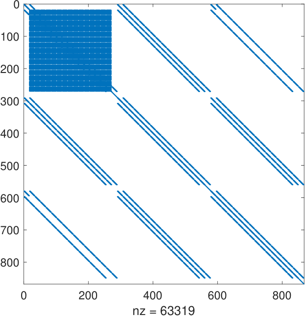
Figure 5: Example 2: convergence of the error H2​(Ω)H^{2}(\Omega) with mesh refinement for different types of discretizations.
Figure 6: Example 2: Decay of energy with respect to time.
Refer to caption
Figure 7: Example 2: Jacobian computed on square mesh without introducing the new variable. It is clear that the number of non-zeros are more than the one proposed in this paper.

6 Conclusion

In this article, we have proposed a numerical technique to solve the time dependent nonlocal plate problem which models deformation of bridge. In order to discretize time dependent part, we need to compute the L2L^{2} projection operator and accordingly, we have modified the VEM space which allows the full computation of the L2L^{2} projection operator. Further, the model problem deals with nonlocal nonlinearity which spoils the sparse structure of the Jacobian matrix and consequently computational cost. We have addressed this difficulty by introducing independent variable and retrieve the sparse structure of the Jacobian. Wellposedness of the fully discrete scheme and a priori error estimates are derived in H2H^{2} norm. Finally, we explore the workability of the numerical technique by examining two benchmark examples including a problem with manufactured solution and clamped boundary condition and another cases are prototype of more realistic bridge modelling without external vertical force functions. Also, we have studied the potential and kinetic energy associated with deformation of bride and plotted against time to demonstrate the uniform decay of energy as time goes to infinity as claimed in [21].

Acknowledgements

The first author was partially supported by the National Agency for Research and Development, ANID- Chile through FONDECYT Postdoctorado project 3200242. The second author was partially supported by the National Agency for Research and Development, ANID-Chile through FONDECYT project 1180913, by projects ACE210010 and Centro de Modelamiento Matemático FB210005 and by DIUBB through project 2120173 GI/C.

References

  • [1] D. Adak, D. Mora, S. Natarajan and A. Silgado, A virtual element discretization for the time dependent Navier-Stokes equations in stream-function formulation, ESAIM Math. Model. Numer. Anal., 55(5), (2021), pp. 2535–2566.
  • [2] D. Adak and S. Natarajan, Virtual element methods for nonlocal parabolic problems on general type of meshes, Adv. Comput. Math., 46(5), (2020), Paper No. 74, 29 pp.
  • [3] D. Adak and S. Natarajan, Virtual element method for semilinear sine-Gordon equation over polygonal mesh using product approximation technique, Math. Comput. Simulation, 172, (2020), pp. 224–243.
  • [4] D. Adak, E. Natarajan and S. Kumar, Convergence analysis of virtual element methods for semilinear parabolic problems on polygonal meshes, Numer. Methods Partial Differential Equations, 35(1), (2019), pp. 222–245.
  • [5] B. Ahmad, A. Alsaedi, F. Brezzi, L.D. Marini and A. Russo, Equivalent projectors for virtual element methods, Comput. Math. Appl., 66, (2013), pp. 376–391.
  • [6] V. Anaya, M. Bendahmane, D. Mora and M. Sepúlveda, A virtual element method for a nonlocal FitzHugh-Nagumo model of cardiac electrophysiology, IMA J. Numer. Anal., 40(2), (2020), pp. 1544–1576.
  • [7] P.F. Antonietti, L. Beirão da Veiga, D. Mora and M. Verani, A stream virtual element formulation of the Stokes problem on polygonal meshes, SIAM J. Numer. Anal., 52, (2014), pp. 386–404.
  • [8] P.F. Antonietti, L. Beirão da Veiga, S. Scacchi and M. Verani, A C1C^{1} virtual element method for the Cahn–Hilliard equation with polygonal meshes, SIAM J. Numer. Anal., 54, (2016), pp. 36–56.
  • [9] P.F. Antonietti, G. Manzini, I. Mazzieri, H.M. Mourad and M. Verani, The arbitrary-order virtual element method for linear elastodynamics models: convergence, stability and dispersion-dissipation analysis, Internat. J. Numer. Methods Engrg., 122(4), (2021), pp. 934–971.
  • [10] E. Artioli, S. de Miranda, C. Lovadina and L. Patruno, A family of virtual element methods for plane elasticity problems based on the Hellinger-Reissner principle, Comput. Methods Appl. Mech. Engrg., 340, (2018), pp. 978–999.
  • [11] E. Bécache, G. Derveaux and P. Joly, An efficient numerical method for the resolution of the Kirchhoff-Love dynamic plate equation, Numer. Methods Partial Differential Equations, 21(2), (2005), pp. 323–348.
  • [12] L. Beirão da Veiga, F. Brezzi, A. Cangiani, G. Manzini, L.D. Marini and A. Russo, Basic principles of virtual element methods, Math. Models Methods Appl. Sci., 23, (2013), pp. 199–214.
  • [13] L. Beirão da Veiga, C. Lovadina and D. Mora, A virtual element method for elastic and inelastic problems on polytope meshes, Comput. Methods Appl. Mech. Engrg., 295, (2015) pp. 327–346.
  • [14] L. Beirão da Veiga, D. Mora and G. Rivera, Virtual elements for a shear-deflection formulation of Reissner-Mindlin plates, Math. Comp., 88, (2019), pp. 149–178.
  • [15] L. Beirão da Veiga, D. Mora and G. Vacca, The Stokes complex for virtual elements with application to Navier-Stokes flows, J. Sci. Comput., 81(2), (2019), pp. 990–1018.
  • [16] D. Bonheure, F. Gazzola and E. Moreira Dos Santos, Periodic solutions and torsional instability in a nonlinear nonlocal plate equation, SIAM J. Math. Anal., 51(4), (2019), pp. 3052–3091.
  • [17] S.C. Brenner and R.L. Scott, The Mathematical Theory of Finite Element Methods, Springer, New York, 2008.
  • [18] F. Brezzi and L.D. Marini, Virtual elements for plate bending problems, Comput. Methods Appl. Mech. Engrg., 253, (2013), pp. 455–462.
  • [19] E. Cáceres and G.N. Gatica, A mixed virtual element method for the pseudostress-velocity formulation of the Stokes problem, IMA J. Numer. Anal., 37, (2017), pp. 296–331.
  • [20] A. Cangiani, G. Manzini and O.J. Sutton, Conforming and nonconforming virtual element methods for elliptic problems, IMA J. Numer. Anal., 37, (2017), pp. 1317–1354.
  • [21] A.D.D. Cavalcanti, M.M. Cavalcanti, W.J. Correa Z. Hajjej, M. Sepúlveda and R. Véjar, Uniform decay rates for a suspension bridge with locally distributed nonlinear damping, J. Franklin Inst., 357(4), (2020), pp. 2388–2419.
  • [22] C. Chinosi and L.D. Marini, Virtual element method for fourth order problems: L2L^{2}-estimates, Comput. Math. Appl., 72(8), (2016), pp. 1959–1967.
  • [23] P.G. Ciarlet, The Finite Element Method for Elliptic Problems, SIAM, 2002.
  • [24] T. Dupont, L2L^{2}-estimates for Galerkin methods for second order hyperbolic equations, SIAM J. Numer. Anal., 10(5), (1973), pp. 880–889.
  • [25] V. Jr. Ferreira, F. Gazzola and E. Moreira Dos Santos, Instability of modes in a partially hinged rectangular plate, J. Differential Equations, 261(11), (2016), pp. 6302–6340.
  • [26] M. Frittelli and I. Sgura, Virtual element method for the Laplace–Beltrami equation on surfaces, ESAIM Math. Model. Numer. Anal., 52, (2018), pp. 965–993.
  • [27] F. Gardini and G. Vacca, Virtual element method for second-order elliptic eigenvalue problems, IMA J. Numer. Anal., 38, (2018), pp. 2026–2054.
  • [28] F. Gazzola, Mathematical Models for Suspension Bridges. Nonlinear Structural Instability, MS&A. Modeling, Simulation and Applications, 15. Springer, Cham, 2018.
  • [29] T. Gudi, Finite element method for a nonlocal problem of Kirchhoff type SIAM J. Numer. Anal., 50(2),(2012), pp. 657-668.
  • [30] F. Lepe, D. Mora, G. Rivera and I. Velásquez, A virtual element method for the Steklov eigenvalue problem allowing small edges, J. Sci. Comput., 88(2), (2021), Paper No. 44, 21 pp.
  • [31] J.L. Lions, Quelques methodes de resolution des problemes aux limites non lineaires, Dunod, Paris (1969).
  • [32] L. Mascotto, I. Perugia and A. Pichler, Non-conforming harmonic virtual element method: hh- and pp- versions, J. Sci. Comput., 77, (2018), pp. 1874–1908.
  • [33] D. Mora and G. Rivera, A priori and a posteriori error estimates for a virtual element spectral analysis for the elasticity equations, IMA J. Numer. Anal., 40, (2020), pp. 322–357.
  • [34] D. Mora, G. Rivera and I. Velásquez, A virtual element method for the vibration problem of Kirchhoff plates, ESAIM Math. Model. Numer. Anal., 52, (2018), pp. 1437–1456.
  • [35] D. Mora and A. Silgado, A C1C^{1} virtual element method for the stationary quasi-geostrophic equations of the ocean, Comput. Math. Appl., (2021), DOI:10.1016/j.camwa.2021.05.022
  • [36] D. Mora and I. Velásquez, Virtual element for the buckling problem of Kirchhoff-Love plates, Comput. Methods Appl. Mech. Engrg., 360, (2020), 112687.
  • [37] I. Perugia, P. Pietra and A. Russo, A plane wave virtual element method for the Helmholtz problem, ESAIM Math. Model. Numer. Anal., 50, (2016), pp. 783–808.
  • [38] G. Vacca, Virtual element method for hyperbolic problems on polygonal meshes, Comput. Math. Appl., 74(5), (2017), pp. 882–898.
  • [39] G. Vacca and L. Beirão da Veiga, Virtual element methods for parabolic problems on polygonal meshes, Numer. Methods Partial Differential Equations, 31(6), (2015), pp. 2110–2134.
  • [40] B. Zhang, Y. Yang and M. Feng, Mixed virtual element methods for elastodynamics with weak symmetry, J. Comput. Appl. Math., 353, (2019), pp. 49–71.