Enhancing the Formation of Wigner Negativity in a Kerr Oscillator via Quadrature Squeezing

Christian Anker Rosiek Thanks: xvm706@alumni.ku.dk

Submitted at the University of Copenhagen on 1 October 2019
Includes minor corrections of February 2022

Abstract

Motivated by quantum experiments with nanomechanical systems, the evolution of a Kerr oscillator with focus on creation of states with a negative Wigner function is investigated. Using the phase space formalism, results are presented that demonstrate an asymptotic behavior in the large squeezing regime for the negativity of a squeezed vacuum state under unitary evolution. The analysis and model are extended to squeezed vacuum states of open systems, adding the decoherence effects of damping and dephasing. To increase experimental relevance, the regime of strong damping is considered. These effects are investigated, yielding similar asymptotic results for the behavior of these effects in the large squeezing regime. Combining these results, it is shown that a weak nonlinearity as compared to damping may be improved by increasing the squeezing of the initial state. It is also shown that this may be done without exacerbating the effects of dephasing.

Contents

Acknowledgments

I thank Albert for allowing me to write this thesis with his help and that of his group. Your trust in my ability has surprised me more than once and allowed and encouraged me to devote my time to a fascinating subject that I have thoroughly enjoyed.

I thank Anders his supervision. I am grateful for the time, energy and ideas you put into the project. I can only assume this to extend far beyond proposal as originally laid out.

A great thanks goes to Massimiliano, without whom the project’s quality would have been substantially diminished. You provided me with the rare combination of technical and companionly support and I enjoyed working with you immensely.

I thank also the other members of SLAB – in no important order, David, Eric, Junxin, Letizia, Mads, Sampo, Yannick, Yeghishe. All of you have contributed to making my work here an enjoyable and learning experience.

I thank Signe and Timo who kept me company in the office and as part of The Breakfast Club. Without you, my time in FK-10 would not have been nearly as compelling or interesting as it was.

I thank my family and friends. Writing a thesis proved a worthy challenge, but I have found none of you to treat me with anything but patience and respect. For that I am greatly indebted. I hope to be able to return this debt should the need ever arise.

In case I forgot to put you here, I did not do so out of spite and I sincerely apologize.

Introduction

Quantum mechanics is a well-established theory to describe the world at microscopic scales. Yet the classical laws of physics are comfortably able to explain most macroscopic phenomena that we can observe. Somewhere in the chain of physical systems of increasing scale, the display of manifestly quantum behavior discontinues as the system transitions to the classical regime. The scale at which this happens varies between systems and an important approach in furthering our understanding of this transition is thus the observation of quantum phenomena in systems of ever increasing scale. The observation of quantum behavior in a macroscopic system could yield fundamental new insights into the relation between quantum and classical mechanics.

The process by which a quantum system loses its quantum properties is called decoherence. The Wigner quasiprobability distribution, introduced [1] to describe quantum corrections to a classical theory, provides a way to describe the state of quantum systems and their coherence. Unlike true probability distributions, the Wigner function can assume negative values and this property is of use in assessing the decoherence of a quantum system. Decoherence effects such as damping lead to the irreversible loss of coherences causing the negativity of the Wigner function to decay [2]. This decay may explain the reduction of system dynamics to adhere to the classical description [3].

As physical systems grow in size, so does the difficulty in preserving their coherence. Nanomechanical oscillators can consist of $10^{13}$ to $10^{14}$ atoms, placing them firmly in the category of macroscopic systems. Thanks to recent advances in nanofabrication technology however, ultra-coherent nanomechanical resonators have been developed [4] that allow for observation of quantum mechanical effects in such macroscopic systems. Examples of experiments demonstrating this include the cooling of a nanomechanical resonator to its ground state [5] and squeezing of mechanical fluctuations below those of the ground state [6]. These experiments demonstrate quantum effects though the states involved have still strictly positive Wigner functions.

To create negativities in the Wigner function, one can consider the evolution of a nonlinear quantum system. A simple such nonlinearity is given by the Kerr effect, which finds application in many quantum experiments and technologies, e.g. the generation of Schrödinger’s cat states [7] and continuous variable quantum computing [8]. In a mechanical system, one can exploit the intrinsic Kerr (Duffing) nonlinearity, present in any mechanical system. For typical mechanical systems however the strength of the nonlinearity is too small when compared to decoherence effects such as damping. Table 1 lists a sample of nonlinear nanomechanical systems, showing that the typical mechanical nonlinearity is several orders of magnitude weaker than the damping of the same system. In such cases it is nontrivial to develop of an experiment demonstrating Wigner negativity.

In this thesis we wish to explore the use of a Kerr nonlinearity to generate states with negative Wigner functions. Guided by the experimental realities, we expect decoherence effects to be a significant impairment and we therefore investigate the use of squeezing to counter this decoherence. We implement in our treatment the decohering effects of damping and dephasing and apply various degrees of squeezing to states of the Kerr Oscillator, studying their evolution and decoherence under damping and dephasing.

The thesis is structured as follows. In Chapters 1 and 2, we review the mathematical fundamentals and the method used for simulating quantum systems. Chapters 3 and 4 contains the main results. Chapter 3 introduces nonlinear oscillators and considers their unitary evolution for selected initial states. This yields understanding of some universal qualities of the evolution of Wigner negativity for a squeezed vacuum state. These will also be important to the later analysis of open systems. Chapter 4 then extends the analysis of its prior chapter to include open systems for the particular case of a squeezed vacuum state.

Table 1: Parameters of nonlinear systems. The table lists the order of magnitude for the base frequency

\omega

, the frequency

g

describing the strength of the Kerr nonlinearity, the damping rate

\gamma

for some experimental nanomechanical resonators. The ratio of

g/\gamma

is important to the viability of generating mechanical states of motion with negative Wigner functions. Parameters given for the Duffing oscillator are converted those of the Kerr oscillator using (3.3) as derived in Appendix A. Theoretical treatments of mechanical resonators are listed in the lower part of the table.

$\omega/2\pi$ (Hz)	$g/2\pi$ (Hz)	$\gamma/2\pi$ (Hz)	$g/\gamma$	System
Experimental systems
$10^{6}$	$10^{-11}$	$10^{-2}$	$10^{-9}$	Silicon nitride membrane [9, 10]
$10^{6}$	$10^{-10}$	$10^{-2}$	$10^{-8}$	Silicon nitride membrane [9, 10]
$10^{6}$	$10^{-4}$	$10^{5}$	$10^{-9}$	Graphene resonator [11]
$10^{6}$	$10^{-2}$	$10^{3}$	$10^{-5}$	Graphene/silicon nitride hybrid resonator [11]
$10^{7}$	$10^{-4}$	$10^{4}$	$10^{-8}$	Nanomechanical resonator [12]
Theoretical treatments
$10^{8}$	$10^{5}$	$100$	$10^{3}$	Cooper pair box coupled to nanomechanical resonator[13]
-	$1$	$10^{5}$	$10^{-3}$	Nanomechanical oscillator [2]
-	1	$1$	$1$	Rescaling of initial state from above [2]

Chapter 1 Fundamentals

Before we study nonlinear systems in later chapters, we spend this chapter reviewing the mathematical techniques used. The first two sections introduces and motivates the use of the simple quantum harmonic oscillator as well as its quantum states. We then describe various unitary operations which may be applied to states and operators of this system: Section 1.3 defines displacement, rotation and squeezing while Section 1.4 and 1.5 describe unitary time evolution and the interaction picture. The introduction to the quantum mechanics of closed systems finishes with a brief look at expectation values motivated by projective measurements. Section 1.7 introduces density matrices and superoperators as required for describing open quantum systems. With this, open system dynamics can now be described. This is done in Section 1.8 in terms of the Markovian master equation. The first half of the chapter then concludes with an example to demonstrate the various techniques and introduce the concept of squeezing.

Once established, the operator formalism is used as a stepping stone to introduce the Wigner quasiprobability distribution and the related phase space formalism. This is a complementary way to describe quantum systems and their dynamics and a therefore translate a selection of the initial sections is therefore translated to this new formalism. The transformation operators are treated in Section 1.11. Section 1.12 introduces two alternate phase space coordinate systems which may help to simplify discussions. Phase space dynamics are treated in Section 1.13 which describes a procedure for translating the master equation of Section 1.8 to a Fokker-Planck-like equation for the Wigner function.

To prepare for the discussion of non-classicality, Section 1.14 describes states and dynamics that are particularly similar to their corresponding classical system. Section 1.15 builds on this and introduces the Wigner current as a way to gain geometrical intuition for the dynamics. Section 1.16 then introduces the two measures which we shall use to gauge non-classicality in this thesis: negative volume and negative peak. After the phase space formalism has been treated in Sections 1.10–1.16, its concepts are applied as Section 1.17 returns to the previous example.

1.1 Quantum Harmonic Oscillator

The simple harmonic oscillator is a system central to the discussion in the thesis. We will follow the conventions of [14] in defining this system and associated mathematical objects.

The harmonic oscillator can be introduced in terms of the generic Hamiltonian for a quantum particle

\hat{H}=\frac{\hat{p}^{2}}{2m}+V(\hat{q}).

(1.1)

The Hamiltonian $\hat{H}$ describes the a harmonic oscillator when the potential is given by

V(\hat{q})=\frac{1}{2}m\omega^{2}\hat{q}^{2},

(1.2)

where $m$ is the mass of the oscillator, $\omega$ is its frequency and $\hat{q}$ and $\hat{p}$ are, respectively, the canonical position and momentum operator of the oscillator. These are Hermitian observables, i.e. $\hat{q}^{\dagger}=\hat{q}$ and $\hat{p}^{\dagger}=\hat{p}.$ They furthermore obey the canonical commutation relation

[\hat{q},\hat{p}]=i\hbar.

(1.3)

We then introduce the annihilation and creation operators $\hat{a}$ and $\hat{a}^{\dagger}$ (collectively known as ladder operators) by a unitary transformation of the position and momentum operators:

	$\hat{a}=\sqrt{\frac{1}{2\hbar m\omega}}\left(m\omega\hat{q}+i\hat{p}\right)$	(1.4a)
and
	$\hat{a}^{\dagger}=\sqrt{\frac{1}{2\hbar m\omega}}\left(m\omega\hat{q}-i\hat{p}\right).$	(1.4b)

The inverse transformations,

\hat{q}=\sqrt{\frac{\hbar}{2m\omega}}(\hat{a}+\hat{a}^{\dagger})\qquad\text{and}\qquad\hat{p}=\frac{1}{i}\sqrt{\frac{\hbar m\omega}{2}}(\hat{a}-\hat{a}^{\dagger}).

(1.5)

allows us to write the Hamiltonian in equation (1.1) in the form

\hat{H}=\hbar\omega\left(\hat{a}^{\dagger}\hat{a}+\frac{1}{2}\right).

(1.6)

From equation (1.3) one has for $\hat{a}$ and $\hat{a}^{\dagger}$ that

\left[\hat{a},\hat{a}^{\dagger}\right]=1.

(1.7)

The number operator $\hat{n}$ can be defined in terms of the ladder operators as

\hat{n}=\hat{a}^{\dagger}\hat{a}.

(1.8)

We also introduce the quadrature operators $\hat{X}$ and $\hat{Y}$ as the Hermitian and anti-Hermitian parts of $\hat{a}$ :

\displaystyle\hat{X}

\displaystyle=\frac{1}{2}\left(\hat{a}+\hat{a}^{\dagger}\right)\,,

\displaystyle\hat{Y}

\displaystyle=\frac{1}{2i}\left(\hat{a}-\hat{a}^{\dagger}\right)\,.

(1.9)

These may be considered dimensionless variants of the position and momentum operators (compare (1.5) and (1.9)). From these expressions and (1.7), the quadrature commutation relation may be derived as

[\hat{X},\hat{Y}]=\frac{i}{2}.

(1.10)

1.2 States of the Harmonic Oscillator

At a given point in time, the system is said to be in a particular state. The state of the system determines the values of all observables at that time. We describe the state of a quantum mechanical system by a ket. For the system in the state denoted by $\Psi$ we write the state of the system as $|\Psi\rangle$ . In this section, we will discuss some important states for the Harmonic oscillator.

The vacuum state is written $|0\rangle$ . It is the lowest energy state of the system so it is also referred to as the ground state and it can be found as the solution to the equation

\hat{a}|0\rangle=0.

(1.11)

Central to any quantum mechanical system are the eigenstates of the system Hamiltonian $\hat{H}$ . For the harmonic oscillator, these states are called number states. Since they are eigenstates of the system Hamiltonian, they are states of definite energy. We construct the $n$ -th number state from the vacuum state $|0\rangle$ by using the creation operator:

|n\rangle=\frac{(\hat{a}^{\dagger})^{n}}{\sqrt{n!}}|0\rangle.

(1.12)

We see that the vacuum state is also the zeroth number state. As the name suggests, the number states are eigenstates of the number operator:

\hat{n}|n\rangle=n|n\rangle.

(1.13)

Applying this to (1.6) shows that $|n\rangle$ is an eigenstate of $\hat{H}$ :

\hat{H}|n\rangle=\hbar\omega\left(n+\frac{1}{2}\right)|n\rangle.

(1.14)

Using (1.7) and (1.12), one may also derive the relations

\hat{a}|n\rangle=\sqrt{n}|n-1\rangle\qquad\hat{a}^{\dagger}|n\rangle=\sqrt{n+1}|n+1\rangle.

(1.15)

The number states form an orthonormal basis for states of the oscillator. Hence, any state $|\Psi\rangle$ can be written as a linear combination of the number states

|\Psi\rangle=\sum_{n=0}^{\infty}c_{n}|n\rangle.

(1.16)

Since they are orthogonal and normalized, we have

\langle n|m\rangle=\delta_{nm},

(1.17)

which can be used to find the coefficient $c_{m}$ as

c_{m}=\langle n|\Psi\rangle.

(1.18)

A state expressed in the form of (1.16) is said to be expanded in the number state basis.

Another important class of states are the coherent states $|\alpha\rangle$ . They may be defined in the number state basis as

|\alpha\rangle=e^{-|\alpha|^{2}/2}\sum_{n}\frac{\alpha^{n}}{\sqrt{n!}}|n\rangle.

(1.19)

Applying $\hat{a}$ to (1.19), $|\alpha\rangle$ is seen to be an eigenstate of the annihilation operator:

\hat{a}|\alpha\rangle=\alpha|\alpha\rangle.

(1.20)

Coherent states are an important class of states in quantum optics. They are often considered to be closest analog to states of the classical harmonic oscillator.

1.3 Transformation Operators

To aid in the manipulation of quantum states, it is useful to define several parameterized unitary transformations.

We introduce first the displacement operator

\hat{D}(\lambda)=e^{\lambda\hat{a}^{\dagger}-\lambda^{*}\hat{a}}.

(1.21)

The exponential function applied to an operator $\hat{A}$ should be interpreted using the Taylor expansion of the exponential function:

e^{\hat{A}}=\sum_{n=0}^{\infty}\frac{\hat{A}^{n}}{n!}.

(1.22)

Applied to the ladder operators, the displacement has the effect [14]


$\displaystyle\hat{D}^{\dagger}(\lambda)\hat{a}\hat{D}(\lambda)$	$\displaystyle=\hat{a}+\lambda,$	(1.23a)
$\displaystyle\hat{D}^{\dagger}(\lambda)\hat{a}^{\dagger}\hat{D}(\lambda)$	$\displaystyle=\hat{a}^{\dagger}+\lambda^{*}.$	(1.23b)

An important theorem for the displacement operator is the disentangling theorem [14]. It states that


$\displaystyle\hat{D}(\lambda)$	$\displaystyle=e^{\lambda\hat{a}^{\dagger}-\lambda^{*}\hat{a}}$	(1.24a)
	$\displaystyle=e^{-\lambda\lambda^{}/2}e^{\lambda\hat{a}^{\dagger}}e^{-\lambda^{}\hat{a}}$	(1.24b)
	$\displaystyle=e^{\lambda\lambda^{}/2}e^{-\lambda^{}\hat{a}}e^{\lambda\hat{a}^{\dagger}}.$	(1.24c)

Applying (1.24b) to the vacuum state, it is seen that the coherent state can also be written as

|\alpha\rangle=\hat{D}(\alpha)|0\rangle.

(1.25)

We next introduce the rotation or phase shift operator

\hat{R}(\phi)=e^{i\hat{n}\phi}.

(1.26)

It adds a complex phase to the ladder operator $\hat{a}$ :


$\displaystyle\hat{R}^{\dagger}(\phi)\hat{a}\hat{R}(\phi)$	$\displaystyle=\hat{a}e^{-i\phi}.$	(1.27a)
$\displaystyle\hat{R}^{\dagger}(\phi)\hat{a}^{\dagger}\hat{R}(\phi)$	$\displaystyle=\hat{a}^{\dagger}e^{i\phi}.$	(1.27b)

The specific instance $\hat{R}(\pi)$ is sometimes called the parity operator [15] since the act of rotating 180° around the origin is the same as the mirroring of all points through the it. We write

\hat{\pi}=\hat{R}(\pi).

(1.28)

Finally we introduce the squeezing operator

\hat{S}(\xi)=e^{\frac{1}{2}\left(\xi^{*}\hat{a}\hat{a}-\xi\hat{a}^{\dagger}\hat{a}^{\dagger}\right)}.

(1.29)

Like the former unitary transformations, $\hat{S}(\xi)$ can be described in terms of its effect on the ladder operators $\hat{a}$ and $\hat{a}^{\dagger}$ :


$\displaystyle\hat{S}^{\dagger}(\xi)\hat{a}\hat{S}(\xi)$	$\displaystyle=\hat{a}\cosh r-\hat{a}^{\dagger}e^{i\theta}\sinh r,$	(1.30a)
$\displaystyle\hat{S}^{\dagger}(\xi)\hat{a}^{\dagger}\hat{S}(\xi)$	$\displaystyle=\hat{a}^{\dagger}\cosh r-\hat{a}e^{-i\theta}\sinh r.$	(1.30b)

The transformations $\hat{D}(\lambda)$ , $\hat{R}(\phi)$ and $\hat{S}(\xi)$ all share the property that their inverse transformation can be found by negating their parameter:


$\displaystyle\hat{D}^{\dagger}(\lambda)$	$\displaystyle=\hat{D}(-\lambda),$	(1.31a)
$\displaystyle\hat{R}^{\dagger}(\phi)$	$\displaystyle=\hat{R}(-\phi),$	(1.31b)
$\displaystyle\hat{S}^{\dagger}(\xi)$	$\displaystyle=\hat{S}(-\xi).$	(1.31c)

1.4 Unitary Dynamics

The time-evolution of a quantum system is determined by the Hamiltonian of the system. Given the system Hamiltonian $\hat{H}$ , the evolution of the state $|\Psi(t)\rangle$ obeys the Schrödinger equation

i\hbar\frac{\partial}{\partial t}|\Psi(t)\rangle=\hat{H}|\Psi(t)\rangle.

(1.32)

If $\hat{H}$ does not vary with time, one can introduce the time-evolution operator

\hat{U}(t)=e^{-i\hat{H}t/\hbar}

(1.33)

to express the evolved state at any point in time $t$ from the initial state $|\Psi(0)\rangle$ :

|\Psi(t)\rangle=\hat{U}(t)|\Psi(0)\rangle.

(1.34)

Dynamics which may be described purely in terms of such a unitary transformation are called unitary dynamics.

A relevant example of unitary dynamics is found in the simple harmonic oscillator. Inserting its Hamiltonian (1.6) into (1.33), the time-evolution operator for the simple harmonic oscillator is found as

\hat{U}(t)=e^{-i\omega(\hat{n}+1/2)t/\hbar}.

(1.35)

$U(t)$ may be recognized as the product of (1.26) and a time dependent complex number of unit magnitude:

\hat{U}(t)=e^{i\omega t/2}\hat{R}(-\omega t).

(1.36)

We may associate the time evolution of the state $|\Psi(0)\rangle$ with a time dependence in the coefficients of the expansion in the number state basis. Applying $\hat{U}(t)$ to each term of (1.19) yields

|\Psi(t)\rangle=\sum_{n=0}^{\infty}c_{n}e^{-i\omega(n+1/2)t}|n\rangle.

(1.37)

1.5 Interaction Picture

In defining the interaction picture, we follow [15]. Consider a Hamiltonian $\hat{H}$ which assumes the form

\hat{H}=\hat{H}_{0}+\hat{V}

(1.38)

where the dynamics for $\hat{H}_{0}$ are exactly solvable in the sense that a basis is known in which $\hat{H}_{0}$ is diagonal (in which case the time evolution of a state $|\Psi(t)\rangle$ may be written in that basis in a form similar to (1.37)). One may now transform the operator $\hat{V}$ to the interaction picture operator $\hat{V}_{I}$ using the transformation

\hat{V}_{I}=e^{i\hat{H}_{0}t/\hbar}\hat{V}e^{-i\hat{H}_{0}t/\hbar}.

(1.39)

In the context of the interaction picture, we refer to $\hat{H}_{0}$ as the base Hamiltonian. We may furthermore define the interaction picture state by

|\Psi(t)\rangle_{I}=e^{i\hat{H}_{0}t/\hbar}|\Psi(t)\rangle.

(1.40)

Given that the state $|\Psi(t)\rangle$ is governed by the Schrödinger equation (1.32), the equation of motion for $|\Psi(t)\rangle_{I}$ will then be

i\hbar\frac{\partial}{\partial t}|\Psi(t)\rangle_{I}=\hat{V}_{I}|\Psi(t)\rangle_{I}.

(1.41)

We see that the operation of transforming to the interaction picture removes $\hat{H}_{0}$ from the dynamics. In quantum optics, the interaction picture with $\hbar\omega(\hat{n}+\frac{1}{2})$ as the base Hamiltonian as referred to as the rotating frame.

For demonstrative purposes, this section denotes quantities in the interaction picture with a subscript $I$ . In the following text, we shall omit the subscript and let the context determine whether a given quantity is consider in the interaction picture.

1.6 Expectation Values and Uncertainties

Measurement is a central concept in quantum mechanics. Here, we use the special case of projective measurements to introduce the statistical properties of a quantum system. Measurable quantities are called observables. Mathematically, an observable is represented by a corresponding Hermitian operator. It is a central axiom in quantum mechanics that the measurement of an observable $\hat{A}$ will always yield a result that is an eigenvalue $A_{i}$ of the corresponding operator. The Hermiticity of $\hat{A}$ ensures that $A_{i}$ is real. After the measurement, the system is found in the matching eigenstate $|A_{i}\rangle$ of the operator.¹¹ 1 For the purposes of this thesis, it is amply sufficient to assume that the eigenstates of the observable are nondegenerate, i.e. that all the eigenstates have distinct eigenvalues. For a broader understanding including degeneracy, one may consult material on quantum measurement [16]. In addition, we take it as an axiom that the eigenstates $|A_{i}\rangle$ of any operator form a basis (though not necessarily orthonormal) in which any state of the system may be expressed exactly.

If the system state before measurement $|\Psi\rangle$ is not an eigenstate of the observable operator, the system is said to collapse to one of the eigenstates. The probability $P(A_{i})$ to measure the outcome $A_{i}$ is given by

P(A_{i})=\left|\langle A_{i}|\Psi\rangle\right|^{2}.

(1.42)

With this, we can determine the expectation value of the operator $\hat{A}$ . This is written

\langle\hat{A}\rangle=\sum_{i}P(A_{i})A_{i}.

(1.43)

For a system in state $|\Psi\rangle$ , the expectation value of $\langle\hat{A}\rangle$ can be calculated as

\langle\hat{A}\rangle=\langle\Psi|\hat{A}|\Psi\rangle.

(1.44)

Since the outcome of a measurement is a stochastic quantity, we can also determine the variance. This is written²² 2 The notation implies that $(\Delta\hat{A})^{2}$ may be viewed as an operator. One should apply this view cautiously since it implies that $\Delta\hat{A}$ depends on the particular state under consideration. Setting e.g. $(\Delta\hat{A})^{2}=(\hat{A}-\langle\Psi|\hat{A}|\Psi\rangle)^{2}$ is consistent with (1.45). The operator $\hat{A}-\langle\Psi|\hat{A}|\Psi\rangle$ is known as the dispersion of $\hat{A}$ [15].

\left\langle(\Delta\hat{A})^{2}\right\rangle=\left\langle\hat{A}{}^{2}\right\rangle-\langle\hat{A}\rangle^{2}.

(1.45)

The derived quantity $\sigma_{\hat{A}}=\sqrt{\left\langle(\Delta\hat{A})^{2}\right\rangle}$ is referred to as the uncertainty of the observable.

One may show that the variances of two observables $\hat{A}$ and $\hat{B}$ obey the inequality [15, 14]

\left\langle(\Delta\hat{A})^{2}\right\rangle\left\langle(\Delta\hat{B})^{2}\right\rangle\geq\frac{1}{4}\left|\langle[\hat{A},\hat{B}]\rangle\right|^{2},

(1.46)

known as Heisenberg’s uncertainty principle. It plays a central role in quantum mechanics. In particular, it states that the product of the variances for two non-commuting observables is nonzero. Two such observables are called incompatible since the system cannot be in a state where both observables have a definite value. (1.46) can be used to derive a series of uncertainty relations between incompatible observables. An important relation of this type is the one between the two orthogonal quadrature operators $\hat{X}$ and $\hat{Y}$ . Using the commutator (1.10) we obtain

\left\langle(\Delta\hat{X})^{2}\right\rangle\left\langle(\Delta\hat{Y})^{2}\right\rangle\geq\frac{1}{16}.

(1.47)

1.7 Mixed States

To increase the relevance of the systems considered, we wish to eventually allow for coupling to an environment. In preparation for the analysis of open systems, we introduce in this section density matrices to represent quantum states.

The density matrix $\hat{\rho}$ of a pure state $|\Psi(t)\rangle$ is formed by taking the outer product between the state ket and bra:

\hat{\rho}=|\Psi(t)\rangle\langle\Psi(t)|.

(1.48)

From the Schrödinger equation (1.32), it is now easy to derive an equation which governs the evolution of $\hat{\rho}$ [17]

\frac{\partial}{\partial t}\hat{\rho}(t)=-\frac{i}{\hbar}\left[\hat{H},\hat{\rho}(t)\right].

(1.49)

(1.49) is usually referred to either as the von Neumann equation. The time-evolution of a state $\hat{\rho}(0)$ explicitly is written using (1.33) as

\hat{\rho}(t)=\hat{U}(t)\hat{\rho}(0)\hat{U}^{\dagger}(t).

(1.50)

So far, the density matrix simply allows for a description of quantum systems. Unlike the representations described in Sections 1.1–1.6 however, a density matrix can be constructed which describes an ensemble of states.

An important example of a mixed state is a state in thermal equilibrium with an environment with a finite temperature $T$ . The temperature of the environment determines for each state of a particular energy, the probability of finding the system in that state. For the harmonic oscillator, the states of definite energy are the number states $|n\rangle$ (see (1.14)). The probability $p(n)$ of finding the system in the state $|n\rangle$ is written

p(n)=\exp\left(-\frac{\hbar\omega n}{k_{B}T}\right)\left[1-\exp\left(-\frac{\hbar\omega}{k_{B}T}\right)\right]^{-1},

(1.51)

where $\omega$ is the oscillator frequency and $k_{B}$ the Boltzmann constant. We construct the density matrix for the thermal state, $\hat{\rho}_{\mathrm{th}}$ , as a linear combination of the number state density matrices $|n\rangle\langle n|$ , each weighted with the matching probability $p(n)$ :

\hat{\rho}_{\mathrm{th}}=\sum_{n}p(n)|n\rangle\langle n|.

(1.52)

It is seen that (1.52) satisfies the requirement that $\langle n|\hat{\rho}_{\mathrm{th}}|n\rangle=p(n)$ . We require for an operator to be a valid density matrix that it is normalized such that

\mathrm{Tr}\hat{\rho}_{\mathrm{th}}=\sum_{n}p(n)=1.

(1.53)

$\mathrm{Tr}$ denotes the trace operation which sums the diagonal elements. It may be carried out in an arbitrary orthonormal basis $|A_{i}\rangle$ :

\mathrm{Tr}\hat{\rho}=\sum_{i}\langle A_{i}|\hat{\rho}|A_{i}\rangle.

(1.54)

The mean occupancy of the thermal state is given by

\langle\hat{n}\rangle=\frac{1}{e^{\hbar\omega/k_{B}T}+1}.

(1.55)

Under unitary system dynamics, mixed state density matrices evolve by (1.49) and (1.50) like pure states. Expectation values of operators with respect to states described by density matrices are also computed with the trace. The expectation value of the operator $\hat{A}$ with respect to the state described by $\hat{\rho}$ is written

\langle\hat{A}\rangle=\mathrm{Tr}\left[\hat{\rho}\hat{A}\right].

(1.56)

Before we end the current section, we note that one can write the equation of motion for $\hat{\rho}$ in analogy with (1.32). To do this, we introduce the superoperator $\mathcal{C}[\hat{O}]$ describing the commutator with the operator $\hat{O}$ :

\mathcal{C}[\hat{O}]\hat{\rho}=[\hat{O},\hat{\rho}].

(1.57)

(1.49) can thus be written

\dot{\hat{\rho}}(t)=-\frac{i}{\hbar}\mathcal{C}[\hat{H}]\hat{\rho}(0).

(1.58)

With $\hat{H}$ constant in time, we can formally write the explicit solution as

\hat{\rho}(t)=e^{(-it/\hbar)\mathcal{C}[\hat{H}]}\hat{\rho}(0).

(1.59)

Additional superoperators will be introduced in the next section.

1.8 Open System Dynamics

So far, the dynamics of the considered quantum systems have been assumed unitary. This assumption implies that the systems are isolated and none of the system degrees of freedom interact with their surroundings. In practice, no physical system is completely isolated from its environment.

Coupling the quantum system to an environment requires an extension of the unitary dynamics of Section 1.4. The evolution of the coupled system is governed by the master equation [18]

\dot{\hat{\rho}}=-\frac{i}{\hbar}[\hat{H},\hat{\rho}]+\gamma\left(\bar{n}+1\right)\mathcal{D}[\hat{a}]\hat{\rho}+\gamma\bar{n}\mathcal{D}[\hat{a}^{\dagger}]\hat{\rho}+\gamma_{\phi}\mathcal{D}[\hat{n}]\hat{\rho}.

(1.60)

The Lindblad superoperator $\mathcal{D}[\hat{O}]$ for an operator $\hat{O}$ acts on the density matrix as

\mathcal{D}[\hat{O}]\hat{\rho}=\hat{O}\hat{\rho}\hat{O}^{\dagger}-\tfrac{1}{2}\hat{O}^{\dagger}\hat{O}\hat{\rho}-\tfrac{1}{2}\hat{\rho}\hat{O}^{\dagger}\hat{O}.

(1.61)

The first term of (1.60) is inherited from the von Neumann equation (1.49). We refer to this term as the unitary part of the system dynamics.

The terms proportional to $\gamma$ in (1.60) produce a damping effect and the frequency $\gamma$ is therefore called the damping coefficient or damping rate. Physically, (4.1) can be used to describe coupling of the system to a thermal bath of bosonic oscillators with a temperature $T$ . We can relate $\bar{n}$ to the temperature of the bath by considering the steady state solution. For the harmonic oscillator, this is assumed to correspond to the thermal equilibrium between system and bath. In thermal equilibrium, the temperature $T$ is shared between system and bath. The mean occupancy the harmonic oscillator is then that of the thermal state (1.52). For the harmonic oscillator, this is given by (1.55). The damping terms of (1.60) can be derived for the harmonic oscillator by considering the combined unitary evolution the system and the thermal equilibrium bath. Tracing out the bath degrees of freedom, then making the Markovian assumption and the rotating wave approximation exactly yields the damping terms [19, 16]. In making the rotating wave approximation, it is assumed that the frequency $\omega$ of the system oscillator is large compared to the frequency describing the interaction between system and bath.

The term $\gamma_{\phi}\mathcal{D}[\hat{n}]\hat{\rho}$ introduces a dephasing effect [20]. In the most narrow sense [21], the effect of dephasing is the decay of the off-diagonal elements of $\hat{\rho}$ expressed in the energy eigenbasis of the system. These elements are called coherences. We assume that the energy levels of any considered system are approximately harmonic and thus take this basis to be the number state basis. The term $\gamma_{\phi}\mathcal{D}[\hat{n}]\hat{\rho}$ is seen to cause decay of the coherences by considering the dephasing-only equation of motion for the $mn$ -matrix element of $\hat{\rho}$ . The right hand side is given by

\langle m|\gamma_{\phi}\mathcal{D}[\hat{n}]\hat{\rho}|n\rangle=-\frac{\gamma_{\phi}}{2}(m-n)^{2}\langle m|\hat{\rho}|n\rangle.

(1.62)

It is seen that the dephasing term leads to exponential decay of the off-diagonal matrix-elements ( $n\neq m$ ) while leaving the diagonal matrix elements ( $n=m$ ) constant.

The effect of the non-unitary terms are collectively known as decoherence.

1.9 Intermission: Quadrature Squeezing

We give now a simple example to better explain the concepts introduced so far. Thus, consider the following Hamiltonian

\hat{H}_{\eta}=i\hbar\left(\eta^{*}\hat{a}^{2}-\eta\left(\hat{a}^{\dagger}\right)^{2}\right),

(1.63)

yielding the von Neumann equation

\dot{\hat{\rho}}=\left[\eta^{*}\hat{a}\hat{a}-\eta\hat{a}^{\dagger}\hat{a}^{\dagger},\hat{\rho}\right].

(1.64)

The Hamiltonian $\hat{H}_{\eta}$ may be obtained as the effective Hamiltonian for a parametric amplifier with a strong coherent drive [18]. With (1.63), we see that the unitary propagator (1.33) can now be written

U(t)=e^{\left(\eta^{*}\hat{a}^{2}-\eta\left(\hat{a}^{\dagger}\right)^{2}\right)t}=S(\xi{=}2\eta t).

(1.65)

To keep the example simple, we consider as initial state the vacuum state $|0\rangle$ . Under the time-evolution of the Hamiltonian (1.63), $|0\rangle$ evolves into the squeezed vacuum state

	$\|\xi\rangle=\hat{S}(\xi)\|0\rangle$	(1.66a)
with a time-dependent squeezing parameter
	$\xi=2\eta t.$	(1.66b)

(1.66) can be regarded as the definition of a squeezed vacuum state.

In the coming sections, we will introduce the phase space formalism which provides a more intuitive understanding of the equations above. Until then though, we can probe the effects of $\hat{H}_{\eta}$ by considering the time-dependence of the quadrature expectation values and variances of the state (1.66a). We do this by expressing the result of applying $\hat{S}$ to the quadrature operators. For simplicity, we choose $\eta$ to be a real number and write $\xi=r=2\eta t=2\eta^{*}t$ . Combining (1.9) and (1.30), we have


$\displaystyle\hat{S}^{\dagger}(r)\hat{X}\hat{S}(r)$	$\displaystyle=\hat{X}e^{-r}\,,$	(1.67a)
$\displaystyle\hat{S}^{\dagger}(r)\hat{Y}\hat{S}(r)$	$\displaystyle=\hat{Y}e^{r}.$	(1.67b)

Applying this, we may determine quadrature expectation values as


	$\displaystyle\left\langle\hat{X}\right\rangle$	$\displaystyle=\langle 0\|\hat{S}^{\dagger}(r)\hat{X}\hat{S}(r)\|0\rangle=0$	(1.68a)
and
	$\displaystyle\left\langle\hat{Y}\right\rangle$	$\displaystyle=\langle 0\|\hat{S}^{\dagger}(r)\hat{Y}\hat{S}(r)\|0\rangle=0,$	(1.68b)

as well as the quadrature variance as


	$\displaystyle\left\langle\left(\Delta\hat{X}\right)^{2}\right\rangle$	$\displaystyle=\langle 0\|\hat{S}^{\dagger}(r)\hat{X}^{2}\hat{S}(r)\|0\rangle=\frac{1}{4}e^{-2r},$	(1.69a)
and
	$\displaystyle\left\langle\left(\Delta\hat{Y}\right)^{2}\right\rangle$	$\displaystyle=\langle 0\|\hat{S}^{\dagger}(r)\hat{Y}^{2}\hat{S}(r)\|0\rangle=\frac{1}{4}e^{2r}.$	(1.69b)

In this case, the variance of the quadrature $\hat{X}$ is reduced or squeezed. The orthogonal quadrature $\hat{Y}$ is called the anti-squeezed quadrature. The effect of $\hat{S}(r)$ is therefore also referred to as quadrature squeezing. We also note that even though the variance of $\hat{X}$ may be made arbitrarily small by choosing a sufficiently large $t$ ,³³ 3 Of course, this purely a theoretical consideration. Experimental factors limit the amount of squeezing that can realistically be achived. the fundamental Heisenberg limit (1.47) is still obeyed due to the matching increase in the variance of $\hat{Y}$ . In the case of vanishing squeezing, the quadrature variances are both $1/4$ .

1.10 The Wigner Quasiprobability Distribution

In the study of classical systems, the concept of a phase space is ubiquitous in modern physics. It provides a concise and abstracted view of system dynamics and allows for the straightforward description of a stochastic system whose state is described by a probability distribution. With the introduction of the Wigner function [1], an analogous concept was made available in the study of quantum systems. The Wigner function shares many properties with a probability distribution in classical phase space, however it can not be viewed as such since it can assume negative values. For this reason it is known as a quasiprobability distribution.

To introduce the Wigner function, we define first the symmetrically ordered characteristic function $\chi(\lambda,\lambda^{*})$ of a state $\hat{\rho}$ by [14]

\chi(\lambda,\lambda^{*})=\mathrm{Tr}[\hat{\rho}e^{\lambda\hat{a}^{\dagger}-\lambda^{*}\hat{a}}]=\mathrm{Tr}[\hat{\rho}\hat{D}(\lambda)]=\langle\hat{D}(\lambda)\rangle

(1.70)

where $\hat{D}(\lambda)$ is given by (1.21). We then define the Wigner function⁴⁴ 4 The Wigner function is an instance of a broader family of phase space qausiprobability distributions [14]. Other important distributions are the Husimi Q function and the Glauber-Sudarshan P function. Except for a brief mention of the Q function in Chapter 4, we will only consider the Wigner function. as the complex Fourier transform of $\chi(\lambda,\lambda^{*})$ :⁵⁵ 5 As exemplified by (1.71), we shall generally omit the limits of integrals when they may be derived from the context. For instance, integrals over the complex phase space coordinates should be taken over the entire phase space. In case of $\lambda$ and $\lambda^{*}$ , this is the set $\mathbb{C}$ .

W(\alpha,\alpha^{*})=\frac{1}{\pi^{2}}\int d\lambda\,d\lambda^{*}\,e^{\lambda^{*}\alpha-\alpha^{*}\lambda}\chi(\lambda,\lambda^{*}).

(1.71)

The characteristic function $\chi(\lambda,\lambda^{*})$ can be recovered from a Wigner function by means of the inverse Fourier transform:

\chi(\lambda,\lambda^{*})=\int d\alpha\,d\alpha^{*}\,e^{\lambda^{*}\alpha-\alpha^{*}\lambda}W(\alpha,\alpha^{*}).

(1.72)

There exists a one-to-one mapping between Wigner functions and density matrices [2]. The inverse of (1.70) is given by [22]

\hat{\rho}=\int d^{2}\lambda\,\chi(\lambda)\hat{D}^{\dagger}(\lambda).

(1.73)

In combination, (1.72) and (1.73) allows one to express the density matrix given a Wigner function. Using the Wigner function expressed in terms of $\alpha$ also allows one to express an expectation value of an operator expression $f(\hat{a},\hat{a}^{\dagger})$ written symmetrically or Weyl ordered [23] in terms of creation and annihilation operators as [14]

\left\langle f(\hat{a},\hat{a}^{\dagger})\right\rangle=\int d\alpha\,d\alpha^{*}\,W(\alpha,\alpha^{*})f(\alpha,\alpha^{*}).

(1.74)

As an example, we derive the Wigner function for the vacuum state $|0\rangle$ . Write the vacuum state Wigner function $W_{|0\rangle}$ as

W_{|0\rangle}(\alpha,\alpha^{*})=\frac{1}{\pi^{2}}\int d\lambda\,d\lambda^{*}\,e^{\lambda^{*}\alpha-\lambda\alpha^{*}}\langle 0|e^{\lambda\hat{a}^{\dagger}-\lambda^{*}\hat{a}}|0\rangle.

(1.75)

Application of the disentangling theorem (1.24) yields

\langle 0|e^{\lambda\hat{a}^{\dagger}-\lambda^{*}\hat{a}}|0\rangle=e^{-\lambda\lambda^{*}/2}\langle 0|e^{\lambda\hat{a}^{\dagger}}e^{-\lambda^{*}\hat{a}}|0\rangle=e^{-|\lambda|^{2}/2}.

(1.76)

This is Fourier transformed to find $W_{|0\rangle}$ as

W_{|0\rangle}(\alpha,\alpha^{*})=\frac{1}{\pi^{2}}\int d\lambda\,d\lambda^{*}\,e^{\lambda^{*}\alpha-\lambda\alpha^{*}}e^{-|\lambda|^{2}/2}=\frac{2}{\pi}e^{-2|\alpha|^{2}},

(1.77)

showing that the Wigner function of the vacuum state is simply a normalized Gaussian function centered at the origin and with variance $1/4$ in both quadrature coordinates.

1.11 Transformations in Phase Space

We can exercise the formalism introduced in the previous section by computing the effect on the Wigner function for the various transformations from Section 1.3. The resulting identities will also be useful later to compute the Wigner function for a state constructed from application of $\hat{D}$ , $\hat{S}$ and $\hat{R}$ to some base state with a known Wigner function.

The argument goes in general as follows: For the transformation $\hat{U}(t)$ (which could be $\hat{D}(\alpha_{0})$ , $\hat{S}(\xi_{0})$ , or $\hat{R}(\phi_{0})$ ) with $t$ as a generic parameter, the Wigner function of the transformed state $\hat{U}(t)\hat{\rho}\hat{U}^{\dagger}(t)$ is written using (1.71). This yields an expression containing a trace of the transformed state with a displacement operator. Using the cyclic property of the trace, the operators are rearranged to transform the displacement operator instead:

\mathrm{Tr}\left[\hat{U}(t)\hat{\rho}\hat{U}^{\dagger}(t)\hat{D}(\lambda)\right]=\mathrm{Tr}\left[\hat{\rho}\hat{U}^{\dagger}(t)\hat{D}(\lambda)\hat{U}(t)\right].

(1.78)

Expanding the displacement operator using its Taylor series (1.22),


$\displaystyle\hat{U}^{\dagger}(t)\hat{D}(\lambda)\hat{U}(t)$	$\displaystyle=\sum_{n}\frac{1}{n!}\hat{U}^{\dagger}(t)(-\lambda^{*}\hat{a}+\lambda\hat{a}^{\dagger})^{n}\hat{U}(t)$	(1.79a)
	$\displaystyle=\sum_{n}\frac{1}{n!}\left(-\lambda^{*}\hat{U}^{\dagger}(t)\hat{a}\hat{U}(t)+\lambda\hat{U}^{\dagger}(t)\hat{a}^{\dagger}\hat{U}(t)\right)^{n}$	(1.79b)
	$\displaystyle=e^{-\lambda^{*}\hat{U}^{\dagger}(t)\hat{a}\hat{U}(t)+\lambda\hat{U}^{\dagger}(t)\hat{a}^{\dagger}\hat{U}(t)}$	(1.79c)

allows for the application of the appropriate identities from Section 1.3 to $\hat{U}^{\dagger}(t)\hat{a}\hat{U}(t)$ and its Hermitian conjugate. The resulting expression is then rewritten to one containing manifestly the Wigner function before transformation which then reveals the transformation’s effect on $W$ .

We first consider the displacement operator $\hat{D}(\alpha_{0})$ from (1.21). We have (making the corresponding density matrix explicit as a subscript of the Wigner function)


$\displaystyle W_{\hat{D}(\alpha_{0})\hat{\rho}\hat{D}^{\dagger}(\alpha_{0})}(\alpha,\alpha^{*})$	$\displaystyle=\frac{1}{\pi^{2}}\int d\lambda\,d\lambda^{}\,e^{\alpha\lambda^{}-\alpha^{*}\lambda}\mathrm{Tr}\left[\hat{D}(\alpha_{0})\hat{\rho}\hat{D}^{\dagger}(\alpha_{0})\hat{D}(\lambda)\right]$	(1.80a)
	$\displaystyle=\frac{1}{\pi^{2}}\int d\lambda\,d\lambda^{}\,e^{\alpha\lambda^{}-\alpha^{}\lambda}\mathrm{Tr}\left[\hat{\rho}e^{-\lambda^{}\hat{a}-\lambda^{}\alpha_{0}+\lambda\hat{a}^{\dagger}+\lambda\alpha_{0}^{}}\right]$	(1.80b)
	$\displaystyle=W_{\hat{\rho}}(\alpha-\alpha_{0},\alpha^{}-\alpha_{0}^{}).$	(1.80c)

Hence applying the displacement operator $\hat{D}(\alpha_{0})$ to a state simply causes its Wigner function to move rigidly in phase space by a distance corresponding to the displacement parameter $\alpha_{0}$ .

Next, consider rotation by an angle $\phi_{0}$ represented by the operator $\hat{R}(\phi_{0})$ of (1.27). Repeating (1.80), we insert the transformed state $\hat{R}(\phi_{0})\hat{\rho}\hat{R}^{\dagger}(\phi_{0})$ into (1.71) and use (1.27) to find


$\displaystyle W_{\hat{R}(\phi_{0})\hat{\rho}\hat{R}^{\dagger}(\phi_{0})}(\alpha,\alpha^{*})$	$\displaystyle=\frac{1}{\pi^{2}}\int d\lambda\,d\lambda^{}\,e^{\alpha\lambda^{}-\alpha^{*}\lambda}\mathrm{Tr}\left[\hat{R}(\phi_{0})\hat{\rho}\hat{R}^{\dagger}(\phi_{0})\hat{D}(\lambda)\right]$	(1.81a)
	$\displaystyle=\frac{1}{\pi^{2}}\int d\lambda\,d\lambda^{}\,e^{\alpha\lambda^{}-\alpha^{}\lambda}\mathrm{Tr}\left[\hat{\rho}e^{-\lambda^{}\exp(-i\phi_{0})\hat{a}+\lambda\exp(i\phi_{0})\hat{a}^{\dagger}}\right]$	(1.81b)
	$\displaystyle\begin{aligned} =\frac{1}{\pi^{2}}\int d\left(\lambda e^{i\phi_{0}}\right)d\left(\lambda e^{i\phi_{0}}\right)^{}\,&\exp\left(\alpha e^{i\phi_{0}}\left(\lambda^{}e^{i\phi_{0}}\right)^{}-\alpha^{}e^{-i\phi_{0}}\left(\lambda e^{i\phi_{0}}\right)\right)\\ &\mathrm{Tr}\left[\hat{\rho}e^{-\lambda^{*}\exp(-i\phi_{0})\hat{a}+\lambda\exp(i\phi_{0})\hat{a}^{\dagger}}\right]\end{aligned}$	(1.81c)
	$\displaystyle=W_{\hat{\rho}}(\alpha e^{i\phi_{0}},\alpha^{*}e^{-i\phi_{0}}).$	(1.81d)

We find that the rotation operator applied to a state causes causes the complex argument of the Wigner function to pick up a corresponding complex phase. Geometrically, this is simply rigid rotation around the origin.

Finally, we may introduce squeezing through a coordinate transformation in the expression for the Wigner function. The transformation of the displacement operator is found using (1.30). For the squeezing parameter $\xi_{0}=r_{0}e^{i\theta_{0}}$ , the argument goes as


$\displaystyle W_{\hat{S}(\xi_{0})\hat{\rho}\hat{S}^{\dagger}(\xi_{0})}(\alpha,\alpha^{*})$	$\displaystyle=\frac{1}{\pi^{2}}\int d\lambda\,d\lambda^{}\,e^{\alpha\lambda^{}-\alpha^{*}\lambda}\mathrm{Tr}\left[\hat{S}(\xi_{0})\hat{\rho}\hat{S}^{\dagger}(\xi_{0})\hat{D}(\lambda)\right]$	(1.82a)
	$\displaystyle\begin{aligned} =\frac{1}{\pi^{2}}\int&d\lambda\,d\lambda^{}\,e^{\alpha\lambda^{}-\alpha^{}\lambda}\\ &\cdot\mathrm{Tr}\left[\hat{\rho}e^{\left(\lambda\cosh r_{0}-\lambda^{}e^{i\theta_{0}}\sinh r_{0}\right)\hat{a}^{\dagger}-\left(\lambda^{*}\cosh r_{0}-\lambda e^{-i\theta_{0}}\sinh r_{0}\right)\hat{a}}\right]\end{aligned}$	(1.82b)
	$\displaystyle\begin{aligned} =\frac{1}{\pi^{2}}\int&d\mu\,d\mu^{}\,e^{\left(\alpha\cosh r_{0}+\alpha^{}e^{i\theta_{0}}\sinh r_{0}\right)\mu^{}-\left(\alpha^{}\cosh r_{0}+\alpha e^{-i\theta_{0}}\sinh r_{0}\right)\mu}\\ &\mathrm{Tr}\left[\hat{\rho}\hat{D}(\mu)\right]\end{aligned}$	(1.82c)
	$\displaystyle=W_{\hat{\rho}}(\alpha\cosh r_{0}+\alpha^{}e^{i\theta_{0}}\sinh r_{0},\alpha^{}\cosh r_{0}+\alpha e^{-i\theta_{0}}\sinh r_{0}).$	(1.82d)

Between (1.82b) and (1.82c), the integral was rewritten in terms of the new coordinates $(\mu,\mu^{*})=(\lambda\cosh r-\lambda^{*}e^{i\theta}\sinh r,\lambda^{*}\cosh r-\lambda e^{-i\theta}\sinh r)$ .

Equations (1.80), (1.81) and (1.82) show that the effect of the operators $\hat{D}(\alpha_{0})$ , $\hat{S}(\xi_{0})$ , or $\hat{R}(\phi_{0})$ can all be expressed simply as coordinate transforms of $W$ .

1.12 Phase Space Coordinates

Refer to caption — Figure 1.1: The Wigner function of the vacuum state. The Wigner function for the vacuum state $|0\rangle$ is a Gaussian function centered at the origin and with an isotropic variance of $1/4$ in the coordinates $(x,y)$ . The expression is shown in (1.86). Note that the used color map displays any value of $W$ below a certain threshold as white.

We will find it useful to express the Wigner function in various coordinate systems. This section establishes the different coordinate systems. Until now, we have considered the Wigner function solely in terms of the coherent amplitude $\alpha$ . For instance, the Wigner function for the vacuum state $|0\rangle$ was found in (1.77) to be

W_{|0\rangle}(\alpha,\alpha^{*})=\frac{2}{\pi}e^{-2|\alpha|^{2}}.

(1.83)

The Wigner function of the vacuum state shall serve to demonstrate the normalization conventions in this section.

We now define the Cartesian or quadrature coordinates $(x,y)$ by

\alpha=x+iy

(1.84)

with real numbers $x$ and $y$ . The relation between $\alpha$ and $(x,y)$ mirrors that between the annihilation operator $\hat{a}$ and the quadrature operators $(\hat{X},\hat{Y})$ (although definitions without this property could have been chosen); compare (1.9) with the inverse relations of (1.84)


$\displaystyle x$	$\displaystyle=\mathrm{Re}\alpha=\frac{1}{2}(\alpha+\alpha^{*}),$	(1.85a)
$\displaystyle y$	$\displaystyle=\mathrm{Im}\alpha=\frac{1}{2i}(\alpha-\alpha^{*}).$	(1.85b)

With the definition (1.84), the vacuum state is expressed in Cartesian coordinates as

W_{|0\rangle}(x,y)=\frac{2}{\pi}e^{-2x^{2}-2y^{2}}.

(1.86)

Writing the Wigner function as a function of two reals $x$ and $y$ , we can visualize it using a density plot. This is done for (1.86) in Figure 1.1. To demonstrate the usefulness of Cartesian coordinates, apply the squeezing transformation $\hat{S}(\xi_{0})$ with $\xi_{0}=r_{0}e^{i\theta_{0}}$ to the Wigner function of the vacuum state. This forms the Wigner function for the squeezed vacuum state (1.66a)

W_{\hat{S}(\xi_{0})|0\rangle}(x,y)=\frac{2}{\pi}\exp\left[-2e^{r_{0}}\left(x\cos\frac{\theta_{0}}{2}+y\sin\frac{\theta_{0}}{2}\right)^{2}-2e^{-r_{0}}\left(x\sin\frac{\theta_{0}}{2}-y\cos\frac{\theta_{0}}{2}\right)^{2}\right]

(1.87)

Finally, polar coordinates are defined by the relation

\alpha=re^{i\phi}

(1.88)

with real numbers $r$ and $\phi$ . In polar coordinates, the vacuum state assumes the form

W_{|0\rangle}(r,\phi)=\frac{2}{\pi}e^{-2r^{2}}.

(1.89)

(1.84) and (1.88) are both each real-valued functions of two real arguments. Choosing these coordinate conventions means that the normalization factor is the same between (1.83), (1.86) and (1.89), e.g.


$\displaystyle 1$	$\displaystyle=\int d\alpha\,d\alpha^{*}\,\frac{2}{\pi}e^{-2\|\alpha\|^{2}}$	(1.90a)
	$\displaystyle=\int dx\,dy\,\frac{2}{\pi}e^{-2x^{2}-2y^{2}}$	(1.90b)
	$\displaystyle=\int_{0}^{\infty}dr\int_{0}^{2\pi}d\phi\,r\,\frac{2}{\pi}e^{-2r^{2}}.$	(1.90c)

This allows one to compare the value of the Wigner function without regard for the coordinates used, e.g.⁶⁶ 6 These definitions also tie back to those of the quadrature operators, defined by (1.9). Other conventions for introducing quadrature operators of dimension $1$ , e.g. $\hat{X}=\frac{1}{\sqrt{2}}\left(\hat{a}+\hat{a}^{\dagger}\right)$ [24] or $\hat{X}=\left(\hat{a}+\hat{a}^{\dagger}\right)$ [18], would cause the peak value of the Wigner function to vary between coordinate systems.

W_{|0\rangle}(r{=}0,\phi{=}0)=W_{|0\rangle}(x{=}0,y{=}0)=W_{|0\rangle}(\alpha{=}0,\alpha^{*}{=}0)=\frac{2}{\pi}.

(1.91)

In some cases, we will also consider vector quantities in this coordinates. To write these, we can introduce the unit vectors for the various coordinates as well. The Cartesian coordinate unit vectors are written⁷⁷ 7 Note that the hat “ $\hat{\cdot}$ ” does not here signify operator quantities. Operator valued vector quantities will not be needed, so any vector marked in this way can be assumed to be a unit vector. $\hat{\mathbf{x}}$ and $\hat{\mathbf{y}}$ while the polar unit vectors are written $\hat{\bm{\phi}}$ and $\hat{\mathbf{r}}$ .

Either one of $\alpha$ , $(x,y)$ , or $(r,\phi)$ refers to a point in phase space. For this reason, we shall refer to $\alpha,x,y,r$ and $\phi$ collectively as spatial coordinates. This should be contrasted with the time coordinate $t$ which naturally enters the discussion when system dynamics are considered.

1.13 Phase Space Dynamics

As noted in Section 1.10, there exists a one-to-one mapping between Wigner functions and density matrices. Because of this, a description of the Wigner function dynamics can be used to uniquely determine the evolution of a system instead of the density matrix dynamics.

In this section, we outline a procedure for deriving the equation of motion for the Wigner function corresponding to the equation of motion for a density matrix. The master equation (1.60) is used here as the most general equation of motion for a density matrix. The master equation may be transformed into a partial differential equation for the Wigner function as is shown below. The goal is to write an equation of the form

\partial_{t}W(\alpha,\alpha^{*},t)=L(\alpha,\alpha^{*},\partial_{\alpha},\partial_{\alpha^{*}})W(\alpha,\alpha^{*},t)

(1.92)

where $L(\alpha,\alpha^{*},\partial_{\alpha},\partial_{\alpha^{*}})$ is a differential operator expression. All differential operators on the right hand side of (1.92) should be spatial ones. To achieve the goal, we follow the procedure of [18].

Take from (1.71) that

W(\alpha,\alpha^{*},t)=\frac{1}{\pi^{2}}\int d\lambda\,d\lambda^{*}\,e^{\lambda^{*}\alpha-\lambda\alpha^{*}}\,\mathrm{Tr}\left[\hat{\rho}(t)e^{\lambda\hat{a}^{\dagger}-\lambda^{*}\hat{a}}\right]

(1.93)

and consider the equation of motion for $W(\alpha,\alpha^{*},t)$ :

\partial_{t}W(\alpha,\alpha^{*},t)=\frac{1}{\pi^{2}}\int d\lambda\,d\lambda^{*}\,e^{\lambda^{*}\alpha-\lambda\alpha^{*}}\partial_{t}\chi(\lambda,\lambda^{*},t).

(1.94)

$\partial_{t}\chi(\lambda,\lambda^{*},t)$ is rewritten by using the relevant equation of motion for the density matrix:

\partial_{t}\chi(\lambda,\lambda^{*},t)=\partial_{t}\mathrm{Tr}\left[\hat{\rho}(t)\hat{D}(\lambda)\right]=\mathrm{Tr}\left[\dot{\hat{\rho}}(t)\hat{D}(\lambda)\right]

(1.95)

Using the cyclic property of the trace, $\mathrm{Tr}\left[\hat{a}\hat{\rho}\hat{D}(\lambda)\right]=\mathrm{Tr}\left[\hat{\rho}\hat{D}(\lambda)\hat{a}\right]$ , the effect of creation and annihilation operators on the displacement operator may be written as differential operators with respect to $\lambda$ and $\lambda^{*}$ . For example

\hat{a}\hat{D}(\lambda)=\hat{a}e^{\lambda\lambda^{*}/2}e^{-\lambda^{*}\hat{a}}e^{\lambda\hat{a}^{\dagger}}=\left(\frac{\partial}{\partial\lambda^{*}}-\frac{\lambda}{2}\right)e^{\lambda\lambda^{*}/2}e^{-\lambda^{*}\hat{a}}e^{\lambda\hat{a}^{\dagger}}=\left(\frac{\partial}{\partial\lambda^{*}}-\frac{\lambda}{2}\right)\hat{D}(\lambda).

(1.96)

Using as appropriate (1.24b) or (1.24c), all relevant combinations of $\hat{D}(\lambda)$ and either $\hat{a}$ and $\hat{a}^{\dagger}$ may be written as [18]


$\displaystyle\hat{a}\hat{D}(\lambda)$	$\displaystyle=\left(-\partial_{\lambda^{*}}+\frac{\lambda}{2}\right)\hat{D}(\lambda),$	(1.97a)
$\displaystyle\hat{a}^{\dagger}\hat{D}(\lambda)$	$\displaystyle=\left(\partial_{\lambda}+\frac{\lambda^{*}}{2}\right)\hat{D}(\lambda),$	(1.97b)
$\displaystyle\hat{D}(\lambda)\hat{a}^{\dagger}$	$\displaystyle=\left(\partial_{\lambda}-\frac{\lambda^{*}}{2}\right)\hat{D}(\lambda),$	(1.97c)
$\displaystyle\hat{D}(\lambda)\hat{a}$	$\displaystyle=-\left(\partial_{\lambda^{*}}+\frac{\lambda}{2}\right)\hat{D}(\lambda).$	(1.97d)

With this, we can write (1.95) with a left hand side of $\partial_{t}\chi(\lambda,\lambda^{*},t)$ and a right hand side consisting of a sum of terms of the form $\lambda^{m}\left(\lambda^{*}\right)^{n}\partial_{\lambda}^{p}\partial_{\lambda^{*}}^{q}\chi(\lambda,\lambda^{*},t)$ . The result is a partial differential equation for the characteristic function $\chi(\lambda,\lambda^{*},t)$ . We apply the Fourier transform (1.93) on both sides. This yields the correct left hand side of (1.92). Each term on the right hand side is rewritten separately. A general right hand side term is rewritten as


$\displaystyle\frac{1}{\pi^{2}}\int d\lambda\,d\lambda^{*}\,$	$\displaystyle e^{\alpha\lambda^{}-\alpha^{}\lambda}\lambda^{m}\left(\lambda^{}\right)^{n}\partial_{\lambda}^{p}\partial_{\lambda^{}}^{q}\left\langle\hat{D}(\lambda)\right\rangle$
	$\displaystyle=\frac{1}{\pi^{2}}(-1)^{m}\partial_{\alpha^{}}^{m}\partial_{\alpha}^{n}\int d\lambda\,d\lambda^{}\,e^{\alpha\lambda^{}-\alpha^{}\lambda}\partial_{\lambda}^{p}\partial_{\lambda^{*}}^{q}\left\langle\hat{D}(\lambda)\right\rangle$	(1.98a)
	$\displaystyle=\frac{1}{\pi^{2}}(-1)^{m+p+q}\partial_{\alpha^{}}^{m}\partial_{\alpha}^{n}\left[\left(\alpha^{}\right)^{q}\alpha^{p}\int d\lambda\,d\lambda^{}\,\partial_{\lambda}^{p}\partial_{\lambda^{}}^{q}e^{\alpha\lambda^{}-\alpha^{}\lambda}\left\langle\hat{D}(\lambda)\right\rangle\right]$	(1.98b)
	$\displaystyle=(-1)^{m+q}\partial_{\alpha^{}}^{m}\partial_{\alpha}^{n}\left[\left(\alpha^{}\right)^{q}\alpha^{p}W(\alpha,\alpha^{*},t)\right].$	(1.98c)

The result is (1.92) with an explicit right hand side.⁸⁸ 8 This derivation of the equation of motion for $W$ uses the corresponding master equation. Alternately, one may disregard the operator picture completely and instead derive Wigner function equation of motion using the symmetrically ordered system Hamiltonian. The right hand side of (1.94) can then be written as a concise expression using the Moyal bracket [25, 26].

As with the master equation, we will normally express any partial differential equation for the Wigner function in the form (1.92) with the left hand side $\partial_{t}W$ and a right hand side containing only spatial derivatives. Statements referring to the left and right hand sides of an equation should be interpreted given the equation in this particular form.

1.14 Gaussian States and Quadratic Hamiltonians

Gaussian states are central to continuous variable quantum mechanics. They may be defined as the set of states whose Wigner function is a Gaussian function [27]. From the inverse Fourier transformation (1.72) it is seen that an equivalent statement is that the characteristic function is a Gaussian function. An important theorem due to Hudson states that only Gaussian states have completely non-negative Wigner functions [28, 29]. Thus any non-Gaussian pure state assumes negative values somewhere in phase space.

We say that a Hamiltonian is quadratic if it consists of terms that are at most quadratic in the ladder operators. We see from this definition that examples of quadratic Hamiltonians include the simple harmonic oscillator (1.6) and parametric squeezing (1.63).

In classical mechanics, one may describe the evolution of a phase space probability density $P$ is described by the Liouville equation.⁹⁹ 9 The appropriate equation of motion for the phase space probability when noise is present is the Fokker-Planck equation. Systems quadratic Hamiltonians have the unique property that the equation of motion for the Wigner function (1.92) assumes a form identical to the classical Liouville equation [30]. Hence the classical and quantum mechanical systems is the same as far as the phase space distributions and the expectation values that may be calculated from them is concerned. Furthermore, any evolution of a Gaussian state with a quadratic Hamiltonian will always result in a Gaussian state. The preservation of the Gaussian quality holds even when adding the damping terms of the master equation (1.60) to the evolution [27] (although not for the dephasing term).

One may show that the equation of motion for the Wigner function (1.92) will contain higher order derivatives if and only if the Hamiltonian contains terms of higher than quadratic order in the annihilation and creation operators [31]. These higher terms are precisely the terms removed when expressing the Liouville equation for the classical system [30].¹⁰¹⁰ 10 Note however, that one can not for unitary evolution connect smoothly the limit $\hbar\to 0$ to the classical case [32, 30]. For this reason, we can also identify these higher order derivatives with the creation of negative regions of the Wigner function.

We note that the unitary transformations $\hat{D}(\lambda)$ , $\hat{R}(\phi)$ , or $\hat{S}(\xi)$ are instances of time evolution operators arising from a quadratic Hamiltonian. Hence, any application of these transformation operators to a Gaussian state results in a Gaussian state as well. In fact, appropriately applying $\hat{D}(\lambda)$ and $\hat{S}(\xi)$ to the vacuum state $|0\rangle$ is sufficient to reach any pure Gaussian state.

1.15 Wigner Current

The classical phase space dynamics as described by the Liouville equation can be formulated as a continuity equation. This is done by defining a current $\mathbf{J}_{P}$ in terms of the probability density $P$ such that the equation of motion equates the time derivative of the density to the negative divergence of the defined current: $\partial_{t}P=-\nabla\cdot\mathrm{J}_{P}$ .

We may define a similar current $\mathbf{J}$ for the Wigner function [33, 34, 35] (also known as the Wigner flow) by choosing $\mathbf{J}$ such that (1.92) can be written

\partial_{t}W=-\nabla\cdot\mathbf{J}.

(1.99)

In (1.99) $W$ takes the role of the classical probability density. For this reason, one might refer to $W$ as the Wigner density.

In the case of quadratic Hamiltonians, the phase space dynamics are unchanged between the classical and quantum mechanical systems. Hence the interpretation of $\mathbf{J}$ is the same as in the classical case. This provides an intuitive geometric view of the evolution of the Wigner function. In contrast to the classical phase space continuity equation, the quantum mechanical expression for $-\nabla\cdot\mathbf{J}$ for a non-quadratic Hamiltonian will contain spatial derivatives of $W$ that are of higher order than $1$ . In that case some freedom (or ambiguity [33]) can arise in choosing $\mathbf{J}$ for the equation of motion for $W$ . Given the presence of such higher-order terms, the dynamics of the Wigner function can not generally be described as a flow of Wigner density along trajectories in phase space [33]. Nevertheless, the expression for $\mathbf{J}$ can in such cases still provide insight into the evolution of the Wigner function.

In fact, these higher order terms will give rise to derivatives of $W$ in the expression of $\mathbf{J}$ . The inclusion of derivatives of $W$ in the expression of $\mathbf{J}$ causes the $\mathbf{J}$ to depend not only on the value of $W$ at the specific point but also on adjacent values. For this reason, terms causing these derivatives to appear in $\mathbf{J}$ can be referred to as non-local terms [33]. As noted in Section 1.14, these higher order derivatives are also a necessary condition for the evolution of a negative Wigner function from a non-negative one.

1.16 Measures of Non-classicality

We define in this section two measures of non-classicality based the negativity of the Wigner function. A Wigner function that assumes negative values in certain parts of phase space is an indicator of non-classicality [14]. Experimentally, negativity of the Wigner function has been used to demonstrate non-classicality [36]. To quantify the amount of negativity here, we introduce two quantities derived from the Wigner function: The negative peak and the negative volume.¹¹¹¹ 11 The terms “volume” and, later, “peak” are used in place of, perhaps, more natural terms such as “integral”, “minimum”, or “maximum”. This is to distinguish from the maximum with respect to variables other than the phase space coordinates. Most commonly, the quantities $\max_{t}\left\{N_{\mathrm{vol}}(t)\right\}$ and $\max_{t}\left\{N_{\mathrm{peak}}(t)\right\}$ which might then be referred to as “maximum negative volume” and “maximum negative peak,” respectively.

We define the negative peak as

N_{\mathrm{peak}}=-\min_{x,y}\left(\min\{0,W(x,y,t)\}\right).

(1.100)

The Wigner function may also be expressed as the expectation value of the displaced parity operator [37]:

W(\alpha,\alpha^{*})=\frac{2}{\pi}\langle\psi|\hat{D}(\alpha)\hat{\pi}\hat{D}^{\dagger}(\alpha)|\psi\rangle.

(1.101)

Writing $\hat{\pi}=e^{i\pi\hat{n}}$ in (1.101) and using the normalization of the displaced state $\hat{D}^{\dagger}(\alpha)|\psi\rangle$ allows one to establish the bounds [22]

-\frac{2}{\pi}\leq W(\alpha,\alpha^{*})\leq\frac{2}{\pi}\qquad\text{for all $\alpha$,}

(1.102)

which by extension bounds $N_{\mathrm{peak}}\leq 2/\pi$ . The upper and lower bounds of (1.101) are for example reached at $\alpha=0$ for the states $|0\rangle$ and $|1\rangle$ respectively.¹²¹² 12 In general, all Wigner functions for pure states with even (odd) wave functions will reach the upper (lower) bound of (1.102) at the origin $\alpha=0$ . This can be seen by considering the definition of $W$ in terms of wave functions [38] or alternately expanding $|\psi\rangle$ in the number state basis in (1.101) and setting $\alpha=0$ . Even (odd) wave function states have contain only even (odd) basis elements in the number state basis. $|0\rangle$ and $|1\rangle$ are trivial examples of such states. For $|0\rangle$ one has from (1.83)

W_{|0\rangle}(\alpha=0)=\frac{2}{\pi}.

(1.103)

To evaluate $W(\alpha=0)$ for the state $|1\rangle$ , use the general expression for the number state Wigner function [14]

W_{|n\rangle}(\alpha,\alpha^{*})=\frac{2}{\pi}(-1)^{n}L_{n}(4|\alpha|^{2})e^{-2|\alpha|^{2}}

(1.104)

and that [39]

L_{1}(x)=1-x.

(1.105)

Combining (1.104) and (1.105), we obtain

W_{|1\rangle}(\alpha=0)=-\frac{2}{\pi}.

(1.106)

The bounds of (1.102) tend to plus and minus infinity as $\hbar\rightarrow 0$ [40]. This behavior is necessary for the Wigner function to agree with the classical phase space probability density in the classical limit (a delta function is an example of a valid classical phase space probability density which obviously violates (1.102) if the bounds remain finite).

The second measure of non-classicality which will be defined is the negative volume $N_{\mathrm{vol}}$ . The negative volume is defined as the integral over all regions where $W$ assumes negative values. We can write this as

N_{\mathrm{vol}}=-\int dx\,dy\,\min\{0,W(x,y,t)\}.

(1.107)

Note that an equivalent definition (used by [29]) is given by

N_{\mathrm{vol}}=\frac{1}{2}\int dx\,dy\,\left(|W(x,y,t)|-W(x,y,t)\right).

(1.108)

$N_{\mathrm{vol}}$ can grow much larger than $N_{\mathrm{peak}}$ . For instance, [29] demonstrate numerically for $0\leq n\leq 250$ that $N_{\mathrm{vol}}$ of the number state $|n\rangle$ increases monotonically with $n$ and approximately as $\tfrac{1}{2}\sqrt{n}$ .

$N_{\mathrm{vol}}$ and $N_{\mathrm{peak}}$ are both functionals of the Wigner function $W$ . Thus they could be written with $W$ (and optionally $t$ ) as their argument. As done above, we will however leave the arguments implicit and interpret them from the context of the symbol.

For a Wigner function that is everywhere non-negative, it follows from their definitions that $N_{\mathrm{vol}}=N_{\mathrm{peak}}=0$ . As soon as the Wigner function departs from this, $N_{\mathrm{vol}}\neq 0$ and $N_{\mathrm{peak}}\neq 0$ . It may be shown that the set of all non-negative Wigner functions and all Wigner functions for Gaussian states (i.e. all Gaussian functions) are equal [28]. Such a theorem does not exist for mixed states however.

As pointed out by [29], the space of all possible states is too large for a single quantity to characterize all non-classical features of a state. In this thesis, the quantities $N_{\mathrm{vol}}$ and $N_{\mathrm{peak}}$ have been chosen to quantify the negativity of a quantum state. Prior use as indicators of non-classicality exists for both negative volume [29, 41] and negative peak [42]. However two wildly differing Wigner functions may still share both $N_{\mathrm{vol}}$ and $N_{\mathrm{peak}}$ . For this reason, we shall also discuss the geometry of the Wigner function and its negative domains supported by plots such as the one found in Figure 1.1.

1.17 Return to Quadrature Squeezing

We return now to the problem Section 1.9 with the tools of the subsequent section. We can gain a better intuition for the system by considering it using the phase space formalism since developed.

We first apply Section 1.13 to derive a partial differential equation for $W(\alpha,\alpha^{*},t)$ . Inserting (1.64) into (1.95), the partial differential equation for the symmetrically ordered characteristic function takes the form


	$\displaystyle\partial_{t}\langle\hat{D}(\lambda)\rangle$	$\displaystyle=\eta^{*}\mathrm{Tr}\left(\left[\hat{a}\hat{a},\hat{\rho}\right]\hat{D}(\lambda)\right)-\eta\mathrm{Tr}\left(\left[\hat{a}^{\dagger}\hat{a}^{\dagger},\hat{\rho}\right]\hat{D}(\lambda)\right)$	(1.109a)
		$\displaystyle=\eta^{*}\mathrm{Tr}\left(\hat{\rho}\left[\hat{D}(\lambda),\hat{a}\hat{a}\right]\right)-\eta\mathrm{Tr}\left(\hat{\rho}\left[\hat{D}(\lambda),\hat{a}^{\dagger}\hat{a}^{\dagger}\right]\right)$	(1.109b)
with the terms of (1.109b) given by

	$\displaystyle\eta^{*}\mathrm{Tr}\left(\hat{\rho}\left[\hat{D}(\lambda),\hat{a}\hat{a}\right]\right)$	$\displaystyle=\eta^{}\left[\left(\partial_{\lambda^{}}+\frac{\lambda}{2}\right)^{2}-\left(-\partial_{\lambda^{*}}+\frac{\lambda}{2}\right)^{2}\right]\mathrm{Tr}\left[\hat{\rho}\hat{D}(\lambda)\right]$	(1.109c)
		$\displaystyle=2\eta^{}\lambda\partial_{\lambda^{}}\mathrm{Tr}\left[\hat{\rho}\hat{D}(\lambda)\right],$	(1.109d)
	$\displaystyle-\eta\mathrm{Tr}\left(\hat{\rho}\left[\hat{D}(\lambda),\hat{a}^{\dagger}\hat{a}^{\dagger}\right]\right)$	$\displaystyle=-\eta\left[\left(\partial_{\lambda}-\frac{\lambda^{}}{2}\right)^{2}-\left(\partial_{\lambda}+\frac{\lambda^{}}{2}\right)^{2}\right]\mathrm{Tr}\left[\hat{\rho}\hat{D}(\lambda)\right]$	(1.109e)
		$\displaystyle=2\eta\lambda^{*}\partial_{\lambda}\mathrm{Tr}\left[\hat{\rho}\hat{D}(\lambda)\right].$	(1.109f)

$\mathrm{Tr}\left(\left[\hat{A},\hat{B}\right]\hat{C}\right)=\mathrm{Tr}\left(\left[\hat{B},\hat{C}\right]\hat{A}\right)$ for operators $\hat{A}$ , $\hat{B}$ and $\hat{C}$ . The result of the calculations (1.109) is written

\partial_{t}\chi(\lambda,\lambda^{*},t)=2\left(\eta^{*}\lambda\partial_{\lambda^{*}}+\eta\lambda^{*}\partial_{\lambda}\right)\chi(\lambda,\lambda^{*},t).

(1.110)

The next step is to convert (1.110) into the equivalent equation of motion for $W(\alpha,\alpha^{*},t)$ . Use (1.71) on both sides of (1.110) to obtain

\partial_{t}W(\alpha,\alpha^{*},t)=\frac{2}{\pi^{2}}\int d\lambda\,d\lambda^{*}\,e^{\lambda^{*}\alpha-\alpha^{*}\lambda}\left(\eta^{*}\lambda\partial_{\lambda^{*}}+\eta\lambda^{*}\partial_{\lambda}\right)\chi(\lambda,\lambda^{*},t).

(1.111)

Then (1.98) is applied to each right hand side term to find

\partial_{t}W(\alpha,\alpha^{*},t)=2\eta^{*}\alpha\partial_{\alpha^{*}}W(\alpha,\alpha^{*},t)+2\eta\alpha^{*}\partial_{\alpha}W(\alpha,\alpha^{*},t).

(1.112)

The effect of this equation becomes more clear, if we write it in Cartesian coordinates instead. Using (1.84), we obtain

\partial_{t}W(x,y;t)=2\left(\mathrm{Re}\eta\,x+\mathrm{Im}\eta\,y\right)\frac{\partial}{\partial x}W\left(x,y,t\right)+2\left(\mathrm{Im}\eta\,x-\mathrm{Re}\eta\,y\right)\frac{\partial}{\partial y}W\left(x,y,t\right).

(1.113)

Using the tools of Section 1.15, we can define a Wigner current $\mathbf{J}$ such that (1.113) takes the form of the continuity-like equation (1.99):

\mathbf{J}=-2\left(\mathrm{Re}\eta\,x+\mathrm{Im}\eta\,y\right)\hat{\mathbf{x}}W\left(x,y,t\right)-2\left(\mathrm{Im}\eta\,x-\mathrm{Re}\eta\,y\right)\hat{\mathbf{y}}W\left(x,y,t\right).

(1.114)

Since the Hamiltonian (1.63) is quadratic, the right hand side of (1.112) contains only first order derivatives. The equation is therefore unchanged from the classical case Liouville equation. Furthermore, the current can be described as flow along trajectories. This may be done by constructing a velocity field $\mathbf{v}$ from (1.114) such that

\mathbf{J}=W\mathbf{v}.

(1.115)

Comparing (1.114) and (1.115) it is seen that $\mathbf{v}$ is independent of $W$ . In other words, $\mathbf{J}$ depends only on the local value of $W$ and not adjacent values. Such non-local dependence would have been expressed using spatial derivatives of $W$ (cf. Section 1.15).

Choosing, as in Section 1.9, a real $\eta$ , the current becomes

\mathbf{J}=-2\eta x\hat{\mathbf{x}}W\left(x,y,t\right)+2\eta y\hat{\mathbf{y}}W\left(x,y,t\right)\qquad\text{for real $\eta$.}

(1.116)

(1.116) describes a flow of density toward the $y$ axis (the term $-2\eta x\hat{\mathbf{x}}$ ) and away from the $x$ axis (the term $2\eta y\hat{\mathbf{y}}$ ). This is intuitively consistent with a decrease in the variance of the quadrature $\hat{X}$ and an increase in the variance of the quadrature $\hat{Y}$ . This evolution in the quadrature variances is exactly the one found in (1.69).

We extend to the general case of a complex $\eta$ by considering the equation of motion in polar coordinates. Using $r$ and $\phi$ of (1.88), we can write

\partial_{t}W(r,\phi,t)=2r\mathrm{Re}\left(\eta e^{-2i\phi}\right)\frac{\partial}{\partial r}W\left(r,\phi,t\right)+2\mathrm{Im}\left(\eta e^{-2i\phi}\right)\frac{\partial}{\partial\phi}W\left(r,\phi,t\right).

(1.117)

To demonstrate the implication of the argument of $\eta$ , we introduce a rotated coordinate system

\phi\rightarrow\phi^{\prime}=\phi+\frac{1}{2}\arg\eta

(1.118)

and a rotated Wigner function

W^{\prime}(r,\phi^{\prime},t)=W^{\prime}(r,\phi^{\prime}-\frac{1}{2}\arg\eta,t).

Inserting into (1.117), we find that $W^{\prime}$ evolves according to the equation of motion

\partial_{t}W^{\prime}(r,\phi^{\prime},t)=2r\mathrm{Re}\left(\eta e^{-i\arg\eta}e^{-2i\phi}\right)\frac{\partial}{\partial r}W\left(r,\phi;t\right)+2\mathrm{Im}\left(\eta e^{-i\arg\eta}e^{-2i\phi}\right)\frac{\partial}{\partial\phi}W\left(r,\phi;t\right)

(1.119)

or equivalently

\partial_{t}W(r,\phi^{\prime},t)=\begin{aligned} 2r\eta^{\prime}\mathrm{Re}\left(e^{-2i\phi^{\prime}}\right)\frac{\partial}{\partial r}&W\left(r,\phi^{\prime},t\right)+2\eta^{\prime}\mathrm{Im}\left(e^{-2i\phi^{\prime}}\right)\frac{\partial}{\partial\phi^{\prime}}W\left(r,\phi^{\prime},t\right)\\ &\text{where $\eta^{\prime}=|\eta|$.}\end{aligned}

(1.120)

We may interpret this as the fact that $W^{\prime}$ evolves under (1.120) as $W$ does under (1.117) for real $\eta$ , i.e. with the current (1.116) (although with the unit vectors rotated correspondingly). Hence the conclusions made from (1.116) for the original non-rotated axes, e.g. the quadrature variance evolution, may be applied unchanged to the axes rotated by $\frac{1}{2}\arg\eta$ .

Note finally, that we can construct a concise analytical expression for the evolution of the vacuum state Wigner function under quadrature squeezing. In Section 1.9, it was established that the system evolves to the squeezed state $|\xi{=}2\eta t\rangle$ as given by (1.66). The Wigner function is then found by inserting the appropriate parameter into the Wigner function for the squeezed vacuum state (1.87):

W(x,y,t)=\begin{aligned} \frac{2}{\pi}\exp\bigg[&-2e^{2|\eta|t}\left(x\cos\frac{\arg\eta}{2}+y\sin\frac{\arg\eta}{2}\right)^{2}\\ &-2e^{-2|\eta|t}\left(x\sin\frac{\arg\eta}{2}-y\cos\frac{\arg\eta}{2}\right)^{2}\bigg].\end{aligned}

(1.121)

The evolution is sketched in Figure 1.2 where the current $\mathbf{J}$ has also been overlayed. The solution is plotted in Figure 1.3. While a trivial example, we nonetheless note that the Wigner function remains non-negative in accordance with the statements in Section 1.14.

This Section illustrates a general method which will be employed later, namely the introduction of a transformed coordinate system and corresponding transformed Wigner function. It also demonstrates the value in being able to freely move between coordinate systems, choosing at any one time the most appropriate one for the problem.

Chapter 2 Numerics

Discussions in the following chapters are supported by the numerical analysis of the discussed physical problems with example parameters. To avoid weighing the discussion down with persistent description of the numerical details, we present in this chapter the techniques used to obtain the numerical results.

The objective of the numerical analysis will often be to compute the Wigner function of a quantum state or some quantity derived from the Wigner function. The state is usually obtained as the result of either unitary (see Section 1.4) or non-unitary (see Section 1.8) evolution given some initial state. Section 1.16 defines the derived quantities which will be used. Section 2.1 describes the steps to simulate quantum systems thereby obtaining. Section 2.2 then details the steps to evaluate the Wigner function at points in phase space and as well as computing its negativity.

The Python library QuTiP [43, 44] (version 4.3) was used to simulate the evolution of the studied quantum systems. We briefly outline the methods used below. We should note however, that QuTiP provides functions abstracting away most of the details in ordinary use.

2.1 Simulation of System Dynamics

Systems are described using the number state basis. To reduce dimensions to a finite number, the basis is truncated and only the lowest $N$ states are considered. A state $|\Psi\rangle$ is then represented by a vector $\vec{c}$ with components $c_{n}$ such that

|\Psi\rangle=\sum_{n=0}^{N-1}c_{n}|n\rangle

(2.1)

given by (1.18) (note the difference to (1.16)). Likewise density matrix can now be represented by an $N$ -by- $N$ matrix $\rho$ with components $\rho_{mn}$ :

\hat{\rho}=\sum_{\begin{subarray}{c}m=0\\ n=0\end{subarray}}^{N-1}\rho_{mn}|m\rangle\langle n|\qquad\text{with}\qquad\rho_{mn}=\langle m|\hat{\rho}|n\rangle.

(2.2)

The states are normalized in the finite basis such that

\sum_{n=0}^{N-1}\left|c_{n}\right|^{2}=1\qquad\text{and}\qquad\sum_{n=0}^{N-1}\rho_{nn}=1.

(2.3)

It is assumed that the magnitude of $c_{n}$ and $\rho_{mn}$ falls off sufficiently fast (see e.g. (1.19) or (3.28)) that the truncation of the basis is a good approximation. An operator $\hat{O}$ is represented by a matrix $O$ with components $O_{mn}$ such that

\hat{O}=\sum_{\begin{subarray}{c}m=0\\ n=0\end{subarray}}^{N-1}O_{mn}|m\rangle\langle n|\qquad\text{with}\qquad O_{mn}=\langle m|\hat{O}|n\rangle.

(2.4)

For an operator expressed in terms of of $\hat{a}$ and $\hat{a}^{\dagger}$ , one may determine $O$ by noting from (1.15) that $\langle m|\hat{a}|n\rangle=\sqrt{n}\delta_{m(n-1)}$ and $\langle m|\hat{a}^{\dagger}|n\rangle=\sqrt{n+1}\delta_{m(n+1)}$ and combining factors of each term by matrix multiplication.

Systems governed by the Schrödinger equation are solved using the time evolution operator $\hat{U}$ of (1.33). Its matrix $U$ is found as the matrix exponential of the matrix for $\hat{H}$ expressed in terms of $\hat{a}$ and $\hat{a}^{\dagger}$ . The evolved state is then obtained with matrix elements given by $\hbox{\hskip 3.95901pt\hskip-3.95901pt\hbox{$\hbox{\hskip 3.95901pt\hskip-3.95901pt\hbox{$U$}\hskip-3.95901pt\hskip 0.0pt\raisebox{-1.2pt}{\hbox{\rule{3.44444pt}{0.32289pt}}}\hskip 0.0pt\hskip 3.95901pt}$}\hskip-3.95901pt\hskip 0.0pt\raisebox{-1.2pt}{\hbox{\rule{3.44444pt}{0.32289pt}}}\hskip 0.0pt\hskip 3.95901pt}\vec{c}$ or $\hbox{\hskip 3.95901pt\hskip-3.95901pt\hbox{$\hbox{\hskip 3.95901pt\hskip-3.95901pt\hbox{$U$}\hskip-3.95901pt\hskip 0.0pt\raisebox{-1.2pt}{\hbox{\rule{3.44444pt}{0.32289pt}}}\hskip 0.0pt\hskip 3.95901pt}$}\hskip-3.95901pt\hskip 0.0pt\raisebox{-1.2pt}{\hbox{\rule{3.44444pt}{0.32289pt}}}\hskip 0.0pt\hskip 3.95901pt}\hbox{\hskip 2.58507pt\hskip-2.58507pt\hbox{$\hbox{\hskip 2.58507pt\hskip-2.58507pt\hbox{$\rho$}\hskip-2.58507pt\hskip 0.0pt\raisebox{-3.14444pt}{\hbox{\rule{3.44444pt}{0.32289pt}}}\hskip 0.0pt\hskip 2.58507pt}$}\hskip-2.58507pt\hskip 0.0pt\raisebox{-3.14444pt}{\hbox{\rule{3.44444pt}{0.32289pt}}}\hskip 0.0pt\hskip 2.58507pt}\hbox{\hskip 3.95901pt\hskip-3.95901pt\hbox{$\hbox{\hskip 3.95901pt\hskip-3.95901pt\hbox{$U$}\hskip-3.95901pt\hskip 0.0pt\raisebox{-1.2pt}{\hbox{\rule{3.44444pt}{0.32289pt}}}\hskip 0.0pt\hskip 3.95901pt}$}\hskip-3.95901pt\hskip 0.0pt\raisebox{-1.2pt}{\hbox{\rule{3.44444pt}{0.32289pt}}}\hskip 0.0pt\hskip 3.95901pt}^{\dagger}$ .

For open systems, the master equation (1.60) is written in element-wise form by applying $\langle m|$ and $|n\rangle$ to both sides:

\dot{\rho}_{mn}=-\frac{i}{\hbar}\langle m|[\hat{H},\hat{\rho}]|n\rangle+\gamma\left(\bar{n}+1\right)\langle m|\mathcal{D}[\hat{a}]\hat{\rho}|n\rangle+\gamma\bar{n}\langle m|\mathcal{D}[\hat{a}^{\dagger}]\hat{\rho}|n\rangle+\gamma_{\phi}\langle m|\mathcal{D}[\hat{n}]\hat{\rho}|n\rangle.

(2.5)

(2.5) is now a system of ordinary differential equations for a finite system of variables $\rho_{mn}$ which may be solved by a standard solve of which QuTiP has a selection to choose from. Simulations in this thesis were computed with ZVODE [45] with the method “BDF”.

Matrices and vectors representing the initial states were obtained by appropriate use of the matrices derived from $\hat{D}$ and $\hat{S}$ in a way similar to $\hat{U}$ . These were used on the vector of the vacuum state and the matrix of a thermal state. The vacuum state vector (2.1) is specified component-wise as $c_{n}=\delta_{0n}$ . In the truncated basis, the thermal state matrix is computed from

\hat{\rho}=\frac{1}{Z}\sum_{n=0}^{N-1}e^{-\hbar\omega n/k_{B}T}|n\rangle\langle n|

(2.6)

where $Z$ is chosen such that (2.3) holds. (2.6) and (1.51–1.52) agree in the limit where $N\to\infty$ .

2.2 Wigner Function and Derived Quantities

QuTiP includes multiple methods for evaluating the Wigner function given a density matrix $\rho$ . The default method which was also used in this thesis employs the Wigner function transition probabilities of the number states.

To evaluate the Wigner function, insert (2.2) into the definition of the Wigner function as given in (1.70–1.71). Rearranging the order of sum, trace and integral yields

W_{\hat{\rho}}(\alpha,\alpha^{*})=\sum_{\begin{subarray}{c}m=0\\ n=0\end{subarray}}^{N-1}\rho_{mn}\frac{1}{\pi^{2}}\int d\lambda\,d\lambda^{*}\,e^{\lambda^{*}\alpha-\alpha^{*}\lambda}\mathrm{Tr}[|m\rangle\langle n|\hat{D}(\lambda)].

(2.7)

Defining $W_{|k\rangle\langle n|}(\alpha,\alpha^{*})$ by

W_{|m\rangle\langle n|}(\alpha,\alpha^{*})=\frac{1}{\pi^{2}}\int d\lambda\,d\lambda^{*}\,e^{\lambda^{*}\alpha-\alpha^{*}\lambda}\mathrm{Tr}[|m\rangle\langle n|\hat{D}(\lambda)]

(2.8)

allows one to write (2.7) as

W_{\hat{\rho}}(\alpha,\alpha^{*})=\sum_{\begin{subarray}{c}m=0\\ n=0\end{subarray}}^{N-1}\rho_{mn}W_{|m\rangle\langle n|}(\alpha,\alpha^{*}).

(2.9)

The quantity $W_{|m\rangle\langle n|}(\alpha,\alpha^{*})$ is referred to as the transition probability. One may show that [46, 26]

W_{|m\rangle\langle n|}(\alpha,\alpha^{*})=\frac{2}{\pi}(-1)^{m}\sqrt{\frac{m!}{n!}}|\alpha|^{(n-m)}e^{-2|\alpha|^{2}}L_{m}^{n-m}(4|\alpha|^{2})e^{i(m-n)\arg\alpha}

(2.10)

where $L_{m}^{n-m}$ denotes the associated Laguerre polynomial. The combination of (2.9) and (2.10) allows one to evaluate the Wigner function.

We will also need to evaluate the quantities $N_{\mathrm{vol}}$ and $N_{\mathrm{peak}}$ defined in Section 1.16. $N_{\mathrm{vol}}$ is computed using a Riemann sum in a bounded region centered on the origin to approximate the definite integral. We define an $N_{x}$ -by- $N_{y}$ grid of points $(x_{i},y_{j})$ and write the distance between adjacent points as


$\displaystyle x_{i+1}-x_{i}$	$\displaystyle=\Delta x,$	(2.11a)
$\displaystyle y_{i+1}-y_{i}$	$\displaystyle=\Delta y.$	(2.11b)

To center the region of integration on the origin, we define the extent of the grid $(x_{\mathrm{ext}},y_{\mathrm{ext}})$ such that


$\displaystyle x_{N_{x}}$	$\displaystyle=x_{\mathrm{ext}}=-x_{1},$	(2.12a)
$\displaystyle y_{N_{y}}$	$\displaystyle=y_{\mathrm{ext}}=-y_{1},$	(2.12b)

Together with (2.11) and (2.12), any two of the three pairs $(N_{x},N_{y})$ , $(x_{\mathrm{ext}},y_{\mathrm{ext}})$ and $(\Delta x,\Delta y)$ specify the grid uniquely. Using the Cartesian coordinates for the Wigner function, the approximation to the integral of $N_{\mathrm{vol}}$ of the state $\hat{\rho}$ is then written as

N_{\mathrm{vol}}=-\sum_{i=1}^{N_{x}}\sum_{j=1}^{N_{y}}\min\left\{0,W_{\hat{\rho}}(x_{i},y_{j})\right\}\Delta x\Delta y.

(2.13)

$W_{\hat{\rho}}(x_{i},y_{j})$ is evaluated using (2.9) and (2.10). $N_{\mathrm{peak}}$ is also evaluated using a grid:

N_{\mathrm{peak}}=-\min_{\begin{subarray}{c}1\leq i\leq N_{x}\\ 1\leq j\leq N_{y}\end{subarray}}\left\{\min\left\{0,W_{\hat{\rho}}(x_{i},y_{j})\right\}\right\}.

(2.14)

To determine a sufficient extent and refinement of the grid, the convergence of the expressions (2.13) and (2.14) were investigated with respect to $N$ , $(\Delta x,\Delta y)$ and $(x_{\mathrm{ext}},y_{\mathrm{ext}})$ separately. In practice, the evaluation of $N_{\mathrm{vol}}$ and $N_{\mathrm{peak}}$ to similar accuracy was found to require similar values of $(\Delta x,\Delta y)$ . Hence, the evaluations performed in (2.13) were reused in the computation of $N_{\mathrm{vol}}$ as given by (2.13). The convergence was assessed with respect to Gaussian states of known negativity ( $N_{\mathrm{vol}}=N_{\mathrm{peak}}=0$ ) and also sample simulated states with nonzero negativity.

Specifically in the case of a squeezed vacuum or thermal state, the necessary minimum values of the parameters $(x_{\mathrm{ext}},y_{\mathrm{ext}})$ are expected vary with the largest variance of the Gaussian function (e.g. the variance of the anti-squeezed quadrature). This was verified for various values of the squeezing parameter $r_{0}$ from the interval $[0.5,2.5]$ .

Chapter 3 Unitary Oscillator Dynamics

The current chapter is dedicated to the understanding of the ways in which the negative regions of the Wigner function form in the Kerr oscillator. We use the phenomenon of nonlinear oscillators in the field of quantum optomechanics to motivate and derive the system Hamiltonian. The rest of the chapter considers exclusively the unitary dynamics of the Kerr oscillator which is general to many quantum systems beside optomechanical ones.

Dynamics general to all initial states are discussed in Section 3.2. In particular, the periodicity of the Kerr oscillator is shown. From there, we move on to study the dynamics of specific initial states, starting with the trivial case of the vacuum state in Section 3.3.

We then consider as initial state the squeezed vacuum state. This state as well as related states form the basis for most discussion in this thesis and a large part of the chapter is therefore dedicated to their treatment. The evolution of the Wigner function and its negativity throughout the period is discussed. We then consider the evolution over short times for which a universal scaling behavior for the negativity is observed and characterized. We also construct a Fourier space solution of the Wigner function for large squeezing.

The conclusions drawn from the squeezed vacuum for short times are readily generalized to thermal states, squeezed below the vacuum state variance. This is done in Section 3.5. The section finishes with a discussion of the applicability to squeezed thermal states that obey the standard quantum limit. Section 3.6 finally considers the coherent state dynamics, serving mainly as perspective for the results obtained for the other initial states.

3.1 Nonlinear Resonators

Nonlinear effects are visible in many physical systems. Within the field of quantum optics they are found systems such as fibers [47] and trapped ions [48]. We focus here on nanomechanical oscillators. These take on many forms [24, 49], including silicon nitride membranes and strings, microtoroidal optomechanical cavities and photonic-phononic systems and Fabry–Pérot cavities with a membrane in the middle or as one of its mirrors. It is common to model each of these systems quantum mechanically as a particle in an harmonic potential (such as (1.2)). Several phenomena can however give rise to an anharmonic potential which can not modeled in this way. In nanonechanical systems, such potential anharmonicities can for example arise from intrinsic material properties, the deformation of the oscillator as it vibrates or electrostatic displacement [50] (see also Table 1). For oscillations that are small in amplitude such as those of quantum fluctuations, the potential takes the form of

V(\hat{q})=\frac{1}{2}m\omega^{2}\hat{q}^{2}+\frac{\beta}{4}\hat{q}^{4}.

(3.1)

This potential describes the Duffing oscillator [51]. The quantity $\beta$ is the Duffing parameter and has appropriate dimensions such that $\beta\hat{q}^{4}$ takes the form of an energy (see Appendix A). For the systems studied in quantum optics, the effects of the harmonic contribution to the potential usually happen on a much shorter time scale than those of the anharmonic contribution (this statement will shortly be formalized as (3.4)). It is therefore useful to consider the system in a rotating frame and with the rotating wave approximation as this removes the harmonic contribution from $\hat{H}$ and simplifies the remaining expression. Practically, the rotating frame expressions are found by transforming to the interaction picture with the base Hamiltonian $\hbar\omega\hat{a}^{\dagger}\hat{a}$ . The rotating wave approximation is then made by removing all terms with an explicit phase that oscillates with a multiple of the base frequency $\omega$ . Appendix A details these steps. The result is a Hamiltonian of the form

\hat{H}=\hbar g\hat{a}^{\dagger}\hat{a}^{\dagger}\hat{a}\hat{a}

(3.2)

where the identification

g=\frac{3\hbar\beta}{8m^{2}\omega^{2}}

(3.3)

has been made. $\hat{H}$ is called the Kerr Hamiltonian.¹¹ 1 Using the commutation relation (1.7) and disregarding added terms proportional two or less ladder operators $\hat{a}^{\dagger}$ and $\hat{a}$ , any expression consisting of two creation and two annihilation operators may be written in the form (3.2). Hence, any such Hamiltonian would be referred to as the Kerr Hamiltonian. Here, we choose to keep the Hamiltonian normal ordered as seen in (3.2). The earlier requirement that the dynamics arising from the harmonic contribution to the potential have much shorter time scales than those from the anharmonic contributions (required for the validity of the rotating wave approximation) can now be expressed as

\omega\gg g.

(3.4)

3.2 Kerr Oscillator

We take now as the system under investigation the Hamiltonian derived in the previous section:

\hat{H}=\hbar g\hat{a}^{\dagger}\hat{a}^{\dagger}\hat{a}\hat{a},

where $\hat{a}$ is the annihilation operator of a bosonic mode and $g$ is the frequency describing the strength of the Kerr nonlinearity. It should be noted that commuting the operators of the first term using the canonical commutation relation (1.7), renders (3.2) in the form

\hat{H}=\hbar g(\hat{n}^{2}-\hat{n}).

(3.5)

In the form of (3.5), $\hat{H}$ is manifestly diagonal in the basis of number states $|n\rangle$ . In other words, $\hat{H}$ shares eigenstates with the harmonic oscillator. It is therefore trivial to apply the time evolution to a state expanded in the number state basis to obtain an expression similar in character to (1.37).

3.2.1 Periodic Evolution

In the operator formalism, evolution of the system can be described with the unitary time-evolution operator. Inserting $\hat{H}$ into (1.33) yields

\hat{U}(t)=e^{-ig(\hat{n}^{2}-\hat{n})t}.

(3.6)

The system evolution is periodic for any initial state which may be seen from the formal solution given an arbitrary initial state $|\Psi(0)\rangle$ . We expand the state in the basis of number states as

|\Psi(0)\rangle=\sum_{n}c_{n}|n\rangle.

(3.7)

Using (1.34) with the expansion of the initial state yields

|\Psi(t)\rangle=\hat{U}(t)|\Psi(0)\rangle=\sum_{n}e^{-ig(n^{2}-n)t}c_{n}|n\rangle.

(3.8)

Inserting $t=\pi/g$ and rewriting the exponential as

e^{-i\pi n^{2}}e^{i\pi n}=(-1)^{n^{2}}e^{i\pi n}=(-1)^{n}e^{i\pi n}=e^{-i\pi n}e^{i\pi n}=1,

(3.9)

it is seen that

|\Psi(\pi/g)\rangle=\sum_{n}e^{-i\pi n}e^{i\pi n}c_{n}|n\rangle=|\Psi(0)\rangle.

(3.10)

Hence the system is periodic with a period of $\pi/g$ .²² 2 In fact any quantum system with discrete energy levels is at least approximately periodic [52]. The analysis of (3.9–3.10) is trivially extended to show exact periodicity (as in (3.10)) for any Hamiltonian which is a polynomial function of $\hat{n}$ . Other systems exhibiting exact periodicity also exists, e.g. the infinite square well.

3.2.2 Generation of Superposition States

Halfway through the period when $t=\pi/2g$ , the system evolves to form a balanced superposition of two instances of the initial state, rotated to be out of phase by 180°. This can be shown by adapting an argument due to [7]. Consider again the evolution of an initial state $|\Psi(0)\rangle$ . Using (3.6), $|\Psi(\pi/2g)\rangle$ is written

|\Psi(\pi/2g)\rangle=e^{-i(\hat{n}^{2}-\hat{n})\pi/2}|\Psi(0)\rangle.

(3.11)

We apply again the expansion in the number state basis to write


$\displaystyle\|\Psi(\pi/2g)\rangle$	$\displaystyle=\sum_{n}e^{-i(n^{2}-n)\pi/2}c_{n}\|n\rangle$	(3.12a)
	$\displaystyle=e^{-i\hat{n}\pi/2}\sum_{n}e^{-in^{2}\pi/2}c_{n}\|n\rangle.$	(3.12b)

Notice now that

e^{-in^{2}\pi/2}=\frac{e^{-i\pi/4}+(-1)^{n}e^{i\pi/4}}{\sqrt{2}}=\begin{cases}-i&\text{$n$ odd,}\\ 1&\text{$n$ even,}\end{cases}

(3.13)

for integer $n$ . Using (3.13) on (3.12b), we continue³³ 3 Alternately, to move from (3.14a) to (3.14c), notice the effect of rotating a number state 180°. Combining (1.12) and (1.27b), we write $\hat{R}(\pi)|n\rangle=(n!)^{-1/2}(\hat{R}(\pi)\hat{a}^{\dagger}\hat{R}^{\dagger}(\pi))^{n}\hat{R}(\pi)|0\rangle=(-1)^{n}|n\rangle$ since $\hat{R}(\pi)\hat{a}^{\dagger}\hat{R}^{\dagger}(\pi)=-\hat{a}^{\dagger}$ and $\hat{R}(\pi)|0\rangle=|0\rangle$ (see e.g. (1.26)).


$\displaystyle\|\Psi(\pi/2g)\rangle$	$\displaystyle=e^{-i\hat{n}\pi/2}\sum_{n}\frac{\left(e^{-i\pi/4}+(-1)^{n}e^{i\pi/4}\right)}{\sqrt{2}}c_{n}\|n\rangle$	(3.14a)
	$\displaystyle=\frac{e^{-i\hat{n}\pi/2}}{\sqrt{2}}\left(e^{-i\pi/4}\sum_{n}c_{n}\|n\rangle+e^{i\pi/4}\sum_{n}e^{-in\pi}c_{n}\|n\rangle\right)$	(3.14b)
	$\displaystyle=\frac{1}{\sqrt{2}}\left(e^{-i\pi/4}e^{-i\hat{n}\pi/2}\|\Psi(0)\rangle+e^{i\pi/4}e^{i\hat{n}\pi/2}\|\Psi(0)\rangle\right).$	(3.14c)

(3.14c) expresses $|\Psi(\pi/2g)\rangle$ as a superposition of the states $e^{-i\hat{n}\pi/2}|\Psi(0)\rangle$ and $e^{i\hat{n}\pi/2}|\Psi(0)\rangle$ . These are, apart from a global phase, exactly a superposition of two instances of the initial state $|\Psi(0)\rangle$ rotated to be 180° out of phase. Note however, that $|\Psi(\pi/2g)\rangle$ may not be a “true superposition”.⁴⁴ 4 Of course, the term “true superposition” is somewhat ill-defined since a change of basis allows any ket to be expressed as a linear combination of more than one basis kets. Here, we shall take the term to mean that the superposition state cannot be written by simply transforming the initial state using the operators of Section 1.3 and addition of a global phase. For example, with a number state as initial state $|\Psi(0)\rangle=|n\rangle$ , we obtain

e^{-i(\hat{n}^{2}-\hat{n})\pi/2}|n\rangle=\frac{1}{\sqrt{2}}\left(e^{-i\pi/4}e^{-in\pi/2}|n\rangle+e^{i\pi/4}e^{in\pi/2}|n\rangle\right)=\sqrt{2}\mathrm{Re}\left(e^{-i\pi/4}e^{-in\pi/2}\right)|n\rangle=|n\rangle,

(3.15)

which is clearly not a state any more exotic than the initial state (it is the initial state). Other examples include the the vacuum state and the superposition formed between the vacuum state and any single other number state.

A less trivial but still nonconforming example is given by the squeezed vacuum state $|\xi\rangle$ as defined in (1.66a). The squeezed vacuum state does not possess continuous rotational symmetry like the number states, but it does exhibit a discrete rotational symmetry of exactly 180°. When $t=\pi/2$ we therefore recover the original state with an added global phase. In the case of the squeezed vacuum state, a nontrivial balanced superposition is however achieved when $t=\pi/8g$ . Evolution of the squeezed vacuum state is examined in Section 3.4.

For a conforming example, the evolution of a coherent state under the Kerr Hamiltonian does generate a superposition at time $t=\pi/2g$ . The periodic evolution of the coherent state is discussed in Section 3.6.1.

3.2.3 Equation of Motion for the Wigner Function

To explore the non-classical aspects of the evolution of the Kerr oscillator, it is useful to study the equation of motion describing the evolution of the Wigner function directly. Starting from the von Neumann equation for the system, one can derive a partial differential equation for the Wigner function which describes the same dynamics. The von Neumann equation for the system at hand is found as

\dot{\hat{\rho}}=-ig\left[\hat{a}^{\dagger}\hat{a}^{\dagger}\hat{a}\hat{a},\hat{\rho}\right]

(3.16)

by insertion of the Kerr Hamiltonian (3.2) into (1.49). Section 1.13 describes a procedure for obtaining the equation of motion for $W$ given (3.16). The result is most easily expressed in polar coordinates (cf. Section 1.12) as

\partial_{t}W(r,\phi,t)=2g\left(r^{2}-1\right)\partial_{\phi}W(r,\phi,t)-\frac{g}{8}\nabla^{2}\partial_{\phi}W(r,\phi,t).

(3.17)

Further details of this derivation may be found in Appendix B. Before we proceed, note that all terms on the right hand side are linear in $g$ . This is expected since $g$ is the only frequency of the problem as is seen in (3.16). This means that system evolution can be considered as a function of a rescaled time

(\text{rescaled time})=gt,

(3.18)

eliminating the parameter $g$ from the system dynamics.

Let us now break down the contents of equation (3.17). It is useful to organize the terms by the order of the spatial derivative of $W$ . Look first to the terms in which first-order spatial derivatives of $W$ appear. These are the terms shared with the classical Liouville equation. The first of these is $2gr^{2}\partial_{\phi}$ . One might describe this as the introduction of a radially dependent angular frequency. It contains purely first-order spatial derivatives and thus causes a flow at every point proportional to the Wigner function at that point. The second term, $-2g\partial_{\phi}$ , is simply an additional oscillator frequency which causes the Wigner function to rotate rigidly in phase space.⁵⁵ 5 The term $-2g\partial_{\phi}W(r,\phi,t)$ corresponds to the right hand side of the simple harmonic oscillator equation of motion. This oscillator has frequency $\omega=-2g$ (see Appendix B). By choosing a frame rotating at the proper frequency, one can change the subexpression $\left(r^{2}-1\right)$ of (3.17) to $\left(r^{2}-k\right)$ for any desired real constant $k$ . The appearance of $1$ could be regarded as the consequence of the choice of the normally ordered Hamiltonian (3.2). Had $\hbar g\hat{a}^{\dagger}\hat{a}\hat{a}^{\dagger}\hat{a}$ been used instead, the $1$ would have vanished. This could also be considered to be an adjustment of the angular frequency of the rotating frame. This term is usually not included in the classical Kerr oscillator, since it is the result of the choice ordering of ladder operators in (3.2).

Since (3.17) describes the unitary evolution, it is expected to contain no even-order spatial derivatives (cf. Section 1.14 or [31]). This is indeed found to be the case. Even-order terms arising from non-unitary evolution will be considered in the next chapter.

The final term $2g\nabla^{2}\partial_{\phi}$ , contains third-order spatial derivatives and is the only term in (3.17) to do so. For this reason, one might say that this term is non-local [33] and indeed, this term describes an effect that cannot be captured in the evolution of a classical phase space probability distribution. Without this term, no negative regions could form in the Wigner function. In case of the Kerr oscillator, this is the only such term.

Equation (3.17) can also be stated as a continuity equation as introduced in Section 1.15. This is done by choosing the Wigner current $\mathbf{J}$ such that (3.17) assumes the form of (1.99). The term $(g/8)\nabla^{2}\partial_{\phi}$ contains both $\partial_{\phi}$ and $\partial_{r}$ so one has some freedom [33] in how to represent it in the expression of $\mathbf{J}$ . The form of (3.17) suggests placing the entire current in the $\phi$ -component of $\mathbf{J}$ though.⁶⁶ 6 There are in fact infinitely many valid choices for distributing the contribution of the term $(g/8)\nabla^{2}\partial_{\phi}$ between $J_{r}$ and $J_{\phi}$ . Reference [33] expresses these choices using a continuous parameter. For the purposes of the current considerations, it is sufficient to simply take the current as being parallel to $\hat{\bm{\phi}}$ . For most quantum states, a large contribution will anyway come from the right hand side term $2g\left(r^{2}-1\right)\partial_{\phi}W$ whose current terms are unambiguously parallel to $\hat{\bm{\phi}}$ . We thus write

\mathbf{J}=\left(-2g\left(r^{2}-1\right)W+\frac{g}{8}\nabla^{2}W\right)r\hat{\bm{\phi}}+0\cdot\hat{\mathbf{r}}.

(3.19)

With this choice of $\mathbf{J}$ , we can view the dynamics as a circular flow around the origin. Supporting this view, the Wigner density $W$ is preserved on rings around the origin [33]:

\partial_{t}\oint d\phi\,W=-\oint d\phi\,\nabla\cdot\mathbf{J}=0.

(3.20)

(3.20) should be treated with caution however, since the current does not evolve independently on each ring. The appearance of $\partial_{r}$ and $\partial_{r}^{2}$ in (3.19) means that current $\mathbf{J}$ on a ring depends on $W$ on adjacent rings. For this reason, the flow in quantum phase space has been called “viscous” [53, 33] when compared to the classical phase space flow.

3.3 Kerr Evolution of Vacuum State

As a trivial example demonstrating the phase space dynamics, consider the vacuum state $|0\rangle$ as initial state. In the operator picture, this is seen to be constant under the time-evolution described by $\hat{U}(t)$ (equations (1.33) and (1.34)):

\hat{\rho}(t)=e^{-ig(\hat{n}^{2}-\hat{n})t}|0\rangle=|0\rangle.

(3.21)

We can draw the same conclusions from the phase space picture. Recall from Section 1.12, the corresponding vacuum state Wigner function

W_{|0\rangle}(r,\phi)=\frac{2}{\pi}e^{-2r^{2}}.

(3.22)

$W_{|0\rangle}(r,\phi)$ is an isotropic Gaussian function centered at the origin and with a variance $\frac{1}{4}$ (measured in both phase space coordinates $x$ and $y$ ). The right hand side of the equation of motion (3.58) is seen to vanish when applied to $W_{|0\rangle}(r,\phi)$ due to the occurrence of the factor

\partial_{\phi}W_{|0\rangle}(r,\phi)=0

(3.23)

in every term. For the initial state

W(r,\phi,0)=W_{|0\rangle}(r,\phi),

(3.24)

one has therefore that

\partial_{t}W(r,\phi,0)=0.

(3.25)

Since the time-evolution of $W(r,\phi,t)$ is governed by a differential equation that is first-order in $t$ , (3.25) completely fixes the evolution of the vacuum state (1.89) to

W(r,\phi,t)=W(r,\phi,0).

(3.26)

This matches the conclusion drawn from (3.21). In geometrical terms it may be concluded by recalling the current $\mathbf{J}$ from (3.19). As seen from this equation, $\mathbf{J}$ describes a flow in the angular direction. Since the vacuum state Wigner function is rotationally invariant: $W_{|0\rangle}(r,\phi)=W_{|0\rangle}(r,0)$ , $\mathbf{J}$ thus leads to no change in $W$ .

3.4 Kerr Evolution of Squeezed Vacuum

We continue with a generalization of the previous example and consider as initial state the squeezed vacuum state of (1.66a):

|\Psi(0)\rangle=|\xi\rangle

(3.27)

The squeezing parameter $\xi$ is written explicitly in terms of its modulus and argument $r_{0}$ and $\theta_{0}$ . The state $|\xi\rangle$ can be expanded in the number-state basis as [23]

|\xi{=}r_{0}e^{i\theta_{0}}\rangle=\frac{1}{\sqrt{\cosh r_{0}}}\sum_{m=0}^{\infty}(-1)^{m}\frac{\sqrt{(2m)!}}{2^{m}m!}e^{im\theta_{0}}\left(\tanh r_{0}\right)^{m}|2m\rangle.

(3.28)

When writing the Wigner function for the squeezed vacuum state, it is convenient to define the parameter $s$ as

s=e^{r_{0}}.

(3.29)

We term $s$ simply “squeezing” to distinguish it from the squeezing parameter $\xi$ . The value of $s$ for the the squeezing parameters $r_{0}$ that we use later are listed in Table 3.1 for reference. The Wigner function for (3.27) can now be found by combining (1.89) and (1.82). In Cartesian coordinates, the resulting initial state Wigner function is written

W_{|\xi\rangle}(x,y)=\frac{2}{\pi}\exp\left(-2s^{2}\left(x\cos\frac{\theta_{0}}{2}+y\sin\frac{\theta_{0}}{2}\right)^{2}-\frac{2}{s^{2}}\left(x\sin\frac{\theta_{0}}{2}-y\cos\frac{\theta_{0}}{2}\right)^{2}\right).

(3.30)

(3.30) defines an elliptical Gaussian function in phase space with its major and minor axes rotated an angle $\theta_{0}/2$ from the $y$ and $x$ axes respectively. This is illustrated in Figure 3.1. Since the equation of motion (3.17) lack dependence on the angular coordinate $\phi$ , the system dynamics are concluded to be rotationally invariant. We may therefore disregard the parameter $\theta_{0}$ and simply set $\theta_{0}=0$ without loss of generality. The change in parameters $s\to 1/s$ and $\theta_{0}\to\theta_{0}+\pi/2$ leaves the Wigner function invariant. Hence the change $s\to 1/s$ also corresponds to a rotation of the phase space coordinate system and we may assume $s\geq 1$ without loss of generality. This leaves us with the initial state

|\Psi(0)\rangle=|\xi{=}r_{0}\rangle

(3.31)

which has the Wigner function

W(x,y,0)=\frac{2}{\pi}e^{-2s^{2}x^{2}-2y^{2}/s^{2}}.

(3.32)

$r_{0}$	$s$
$0.5$	$1.65$
$0.75$	$2.12$
$1$	$2.72$

$r_{0}$	$s$
$1.25$	$3.49$
$1.5$	$4.48$
$1.75$	$5.75$

$r_{0}$	$s$
$2$	$7.39$
$2.25$	$9.49$
$2.5$	$12.18$

Table 3.1: Relation between often used squeezing parameters and squeezing. The relation between the squeezing parameter

r_{0}

and the squeezing

s=\exp r_{0}

is defined by (3.29).

3.4.1 Periodic Evolution

As stated in Section 3.2.1, the unitary evolution described by (3.8) is periodic with period $\pi/g$ . In particular, the periodicity of squeezed vacuum state evolution is just $\pi/4g$ . Re-purposing the arguments in Section 3.2.1, this is shown as follows: Consider the squeezed state in the number state basis (3.28). For this derivation, it is sufficient that the squeezed vacuum state contains only even terms in its expansion in the number state basis. That this is the case can be seen from (3.28). We shall express it here simply as

|\Psi(0)\rangle=\sum_{m}c_{2m}|2m\rangle.

(3.33)

The time evolution follows from (3.6) and (3.33) as

|\Psi(t)\rangle=\hat{U}(t)|\Psi(0)\rangle=\sum_{m}e^{-ig(4m^{2}-2m)t}c_{2m}|2m\rangle.

(3.34)

We evolve the state to a time $t=\pi/4g$ using (3.6) to find

|\Psi(\pi/4g)\rangle=\sum_{m}e^{-i(m^{2}-m/2)\pi}c_{2m}|2m\rangle=e^{-i\hat{n}\pi/4}\sum_{m}e^{-i(m^{2}-m)}c_{2m}|2m\rangle.

(3.35)

Using the identity (3.9), we now have

|\Psi(\pi/4g)\rangle=e^{-i\hat{n}\pi/4}\sum_{m}c_{2m}|2m\rangle=e^{-i\hat{n}\pi/4}|\Psi(0)\rangle=\hat{R}(-\frac{\pi}{4})|\Psi(0)\rangle.

(3.36)

We see from (3.36) that the squeezed vacuum state exhibits a periodicity of only $\pi/4g$ (compared to the general periodicity of $\pi/g$ , see Section 3.2.1). The periodicity can be seen demonstrated in Figure 3.2.

When time reaches a certain rational multiple of the period, special states are observed. These are somewhat reminiscent of the fractional revival states found when considering a coherent state evolving with the same dynamics (see also Section 3.6). Specifically at time $t=\pi/8$ , the system state is a coherent superposition of two squeezed vacuum states. To show this we re-purpose the arguments of Section 3.2.1. Applying the time evolution operator (3.6) to the expansion in number states (3.33), we obtain

|\Psi(\pi/4g)\rangle=\sum_{m}e^{-i(4m^{2}-2m)\pi/8}c_{2m}|2m\rangle=e^{i\hat{n}\pi/8}\sum_{m}e^{-im^{2}\pi/2}c_{2m}|2m\rangle.

(3.37)

Then apply (3.13) to obtain


$\displaystyle\|\Psi(\pi/4g)\rangle$	$\displaystyle=e^{i\hat{n}\pi/8}\sum_{m}\frac{\left(e^{-i\pi/4}+(-1)^{m}e^{i\pi/4}\right)}{\sqrt{2}}c_{2m}\|2m\rangle$	(3.38a)
	$\displaystyle=\frac{e^{i\hat{n}\pi/8}}{\sqrt{2}}\left(e^{-i\pi/4}\sum_{m}c_{2m}\|2m\rangle+e^{i\pi/4}\sum_{m}e^{-im\pi}c_{2m}\|2m\rangle\right)$	(3.38b)
	$\displaystyle=\frac{1}{\sqrt{2}}\left(e^{-i\pi/4}e^{i\hat{n}\pi/8}\|\Psi(0)\rangle+e^{i\pi/4}e^{-3i\hat{n}\pi/8}\|\Psi(0)\rangle\right).$	(3.38c)

We thus see that the state evolves to a coherent superposition of the states $e^{i\hat{n}\pi/8}|\Psi(0)\rangle$ and $e^{-3i\hat{n}\pi/8}|\Psi(0)\rangle$ . These are both instances of the initial state $|\Psi(0)\rangle=|\xi\rangle$ but rotated 90° out of phase. This state can also be seen in Figure 3.2.

3.4.2 Negativity during a Full Period

We now wish to characterize the evolution of negativity for the state. To this end, $N_{\mathrm{vol}}$ and $N_{\mathrm{peak}}$ have been plotted for an entire period in Figure 3.3.

(a) Negative volume

(b) Negative peak

Figure 3.3: Negativity during periodic evolution of squeezed vacuum. The initial states are squeezed vacuum states with varying squeezing parameters

r_{0}

. To reduce clutter, the graph of negative peak has been limited to a few different choices of

r_{0}

We consider first the negative volume $N_{\mathrm{vol}}$ . For larger squeezing parameters, the negative volume increases rapidly until it reaches a plateau. The plateau becomes more clear as $r_{0}$ increases and the $N_{\mathrm{vol}}$ as a function of time takes on a more square appearance. As the squeezing increases, $N_{\mathrm{vol}}$ additionally starts to fluctuate strongly and an increasing finer structure of details appear in the plateau region. At special points in time even larger features of $N_{\mathrm{vol}}$ become visible. This is most evident when $gt=\pi/8$ and (to a lesser degree) when $gt=\pi/12$ . Here, a dip in the negative volume can be clearly made out. The Wigner functions of these special states can be seen in Figure 3.2. The height of the plateau appears to scale roughly quadratically with $r_{0}$ (though not exactly). Figure 3.4 shows the height of the plateau $\max_{t}\left\{N_{\mathrm{vol}}(t)\right\}$ as a function of the squared squeezing parameter $r_{0}^{2}$ for $r_{0}\in[0,2.5]$ .

Figure 3.4: Maximum negative volume for varying squeezing. The maximum negative volume

\max_{t}\{N_{\mathrm{vol}}(t)\}

was computed from the simulations in Figure 3.3a. The quantity scales roughly quadratically with

r_{0}

. The dotted line is a linear function of

r_{0}

to guide the eye.

We next consider the negative peak $N_{\mathrm{peak}}$ . This is shown for a full period in Figure 3.3b. $N_{\mathrm{peak}}$ generally increases with squeezing until around $r_{0}=1$ . Further increasing the squeezing from $r_{0}=1$ increases the frequency and amplitude of the fluctuations but does not apparently increase the peak negativity. Within the investigated parameter regime, the peak negativity does not reach the bound of $2/\pi=0.637$ set by (1.102). As with $N_{\mathrm{vol}}$ , the points $gt=\pi/8$ and $gt=\pi/12$ can be made out as dips in the graph of $N_{\mathrm{peak}}$ .

Some behavior is shared between $N_{\mathrm{vol}}$ and $N_{\mathrm{peak}}$ . Both start with a value of zero at $t=0$ . This is expected since the initial state is a Gaussian state. As the time first evolves, they both increase rapidly and monotonically for some time. After that, the evolution changes character and the negativity does not clearly increase or decrease. We are mainly interested in this initial evolution of the negativity where the rate at which the negativity grows increases significantly with squeezing.

3.4.3 Evolution over Short Time

We anticipate that the decoherence effects introduced in Chapter 4 will have a diminishing effect on the negativity, in some cases causing the negativity to completely vanish before the plateau. Hence, we shall focus on the initial stages of evolution. Figure 3.3 demonstrates that the rate of growth for the negativity increases with squeezing and thus indicates that it may be possible to compensate for strong decoherence effects by using states of stronger squeezing.

Figure 3.13 shows the time-evolution of the squeezed state state $|\xi{=}1.5\rangle$ over short times. Analogously to the classical evolution of a probability density [54], the squeezed state evolves to form an “S”-like shape in phase space. Unlike the classical evolution however, negative and positive fringes appear in the concave regions of the S-shape. These fringes constitute the negative regions of the Wigner function. As the state evolves, the fringes increase in number and amplitude as the curve of the S-shape becomes more pronounced. Figure 3.7 shows the negativity in the initial stages of evolution, demonstrating that this corresponds to a growth in negativity.

A geometrical understanding of the short time behavior is gained by considering the Wigner current (3.19) for the initial state (3.32) along the $y$ -axis. In Cartesian coordinates, the current for the initial state on the $y$ -axis ( $x=0$ ) reads

\displaystyle\mathbf{J}

\displaystyle=g\left[s^{2}+s^{-2}+1+2(1-s^{-4})y^{2}\right]yW(0,y,0)\hat{\mathbf{x}}.

(3.39)

The bending of the shape is caused by the terms not linear in $y$ , i.e. $2g(1-s^{-4})y^{3}W(0,y,0)\hat{\mathbf{x}}$ . This dependence on $y^{3}$ is illustrated in Figure 3.6.

(a) Negative volume

(b) Negative peak

Figure 3.7: Negativity during short time unitary evolution of squeezed vacuum. The initial states are squeezed vacuum states with varying

r_{0}

. The evolution of

N_{\mathrm{vol}}

and

N_{\mathrm{peak}}

appear qualitatively similar in that an increase in

r_{0}

causes the negativity to initially grow more rapidly. The short time evolution is discussed in Section 3.4.3.

3.4.4 Preliminary Algebraic View of Negativity

We shall now try to build up some intuition for the scaling of negativity. Let us start by considering the evolution of the squeezed vacuum state $|\Psi(0)\rangle$ where

|\Psi_{\xi}(0)\rangle=\hat{S}(r_{0})|0\rangle.

(3.40)

We can write the time-evolution of the state as

|\Psi_{\xi}(0)\rangle=\hat{U}(t)|\Psi_{\xi}(0)\rangle

(3.41)

with the time evolution operator obtained by combining (3.6) and (3.33) as

\hat{U}(t)=e^{-ig\hat{a}^{\dagger}\hat{a}^{\dagger}\hat{a}\hat{a}t}.

(3.42)

The squeezing transformation $\hat{S}(\xi^{\prime})$ for any choice of the parameter $\xi^{\prime}$ leaves the negativity unchanged as can be seen by applying (1.82) to the definitions (1.100) and (1.107). Computing the negativity of the state $|\Psi_{\xi}(t)\rangle$ is thus the same as computing the negativity of the state $\hat{S}^{\dagger}(r_{0})|\Psi_{\xi}(t)\rangle$ , i.e.

N_{\mathrm{vol}}[|\Psi_{\xi}(t)\rangle]=N_{\mathrm{vol}}[\hat{S}^{\dagger}(\xi)|\Psi_{\xi}(t)\rangle]=N_{\mathrm{vol}}\left[\hat{S}^{\dagger}(r_{0})\hat{U}(t)\hat{S}(r_{0})|0\rangle\right],

(3.43)

writing the state explicitly as an argument to $N_{\mathrm{vol}}$ . Equation (3.43) moves the squeezing parameter $r_{0}$ from the initial state to the equation of motion. The squeezing transformation applied to $\hat{a}$ may be stated as [14]

\displaystyle\hat{S}(r_{0})\hat{a}\hat{S}^{\dagger}(r_{0})

\displaystyle=\hat{X}s+i\hat{Y}s^{-1}

(3.44)

and the operator part of the Kerr Hamiltonian thus transforms as

\displaystyle\hat{S}(r_{0})\hat{a}^{\dagger}\hat{a}^{\dagger}\hat{a}\hat{a}\hat{S}^{\dagger}(r_{0})

\displaystyle=\left(\hat{X}s+i\hat{Y}s^{-1}\right)^{2}\left(\hat{X}s-i\hat{Y}s^{-1}\right)^{2}.

(3.45)

Keeping only the highest power of $s$ in (3.45), we arrive at

\hat{S}(r_{0})\hat{a}^{\dagger}\hat{a}^{\dagger}\hat{a}\hat{a}\hat{S}^{\dagger}(r_{0})\xrightarrow[s\to\infty]{}s^{4}\hat{X}^{4}.

(3.46)

We expect then that the dynamics are dominated by the term proportional to $s^{4}$ in the limit of large squeezing. We shall summarize this statement symbolically by writing (3.43) as

N_{\mathrm{vol}}\left[|\Psi_{\xi}(t)\rangle\right]\approx N_{\mathrm{vol}}\left[e^{-igts^{4}\hat{X}^{4}}|0\rangle\right]\qquad\text{for large $s$.}

(3.47)

Here, the squeezing transformation (3.46) was applied to the Taylor expansion of $\hat{U}(t)$ as in (1.79). The derivation (3.43–3.47) may be repeated for $N_{\mathrm{peak}}$ to similarly write

N_{\mathrm{peak}}\left[\Psi_{\xi}(t)\right]\approx N_{\mathrm{peak}}\left[e^{-igts^{4}\hat{X}^{4}}|0\rangle\right]\qquad\text{for large $s$.}

(3.48)

Hence, having disregarded all but the leading order terms in the expressions for $N_{\mathrm{vol}}$ and $N_{\mathrm{peak}}$ , it could be suggested that the negativity for a highly squeezed initial state is constant as a function of the quantity $gts^{4}$ . With (3.47) and (3.48), we have however no indication of the validity of (3.46). Applying an analogous transformation directly to the Wigner function and phase space dynamics yields greater insight into the meaning of (3.46). Before this is done however, we first view the problem in a geometric setting.

3.4.5 Preliminary Geometric View of Negativity

An estimate similar to (3.47) may be reached by considering geometrically the time-evolution in the phase space picture. We consider again as the initial state a highly squeezed vacuum state. The initial state is displayed in Figure 3.8a. Let the squeezed state evolve over a short time so that it forms an S-shape in phase space as displayed in Figure 3.8b. It is known from simulations (recall Figure 3.5) that the negative parts of the Wigner function first appear as fringes in the concave region of the S-shape. We might intuitively expect the time at which the negativity first appears to bear some relation to the magnitude of the initial state squeezing (e.g. for no squeezing, no negativity will be observed). To support this, let us apply some dimensions to Figure 3.8a. For the initial state, we may define two characteristic phase space-length scales from the variances in the anti-squeezed and squeezed direction.⁷⁷ 7 Of course, these quantities, as displayed in Figure 3.8, are “lengths” in phase space coordinates and are therefore both dimensionless. It is possible to use a Wigner function where the arguments have differing dimensions (indeed this was the case when the function was first introduced by Eugene Wigner in 1932 [1]) making it manifestly impossible to compare lengths measured in anything but parallel directions in phase space. Here, however, we compare lengths in parallel directions since the length proportional to $s$ is transformed to a length in its orthogonal direction using the equation of motion of a particle. Thus only lengths measured in parallel directions are compared as can be clearly seen in Figure 3.8b. In terms of the parameter $s$ , these characteristic length scales are⁸⁸ 8 The aforementioned variances are actually given by $s^{2}/4$ and $1/4s^{2}$ cf. equations (1.69a) and (1.69b). The constant factor $\sqrt{1/4}$ may be absorbed into $k_{0}$ when they are compared in (3.51). $s$ and $s^{-1}$ .

Consider now the hypothetical motion of a classical particle⁹⁹ 9 A related concept is the Ehrenfest time $t_{E}$ [30]. It is a time until which evolution leaves classical and quantum mechanical phase space distributions in general agreement. placed a distance $s$ up from the origin in the anti-squeezed direction. We can find the instantaneous phase space velocity of the particle from the classical probability current. The classical current is found by removing all derivative expressions from $\mathbf{J}$ of (3.19). The result can be written as

\mathbf{J}=W\mathbf{v}

(3.49)

where $\mathbf{v}$ is a vector quantity independent of the value of $W$ . $\mathbf{v}$ corresponds to the phase space velocity of a classical particle: $\mathbf{v}=(\dot{x},\dot{y})$ . From (3.19) we obtain

\mathbf{v}=-2g\left(r^{2}-1\right)r\hat{\bm{\phi}}.

Evaluating $\mathbf{v}$ at the position of the particle $(x,y)=(0,s)$ yields

\displaystyle(\dot{x},\dot{y})

\displaystyle\propto(2gs^{3},0)

(3.50)

where the term $2gsr$ has been neglected from $\dot{x}$ due to the assumption of large squeezing $s$ . $(\dot{x},\dot{y})$ is displayed as an arrow in Figure 3.8a. We expect some amount negativity to appear once the particle has moved some fixed multiple of the squeezed width $l_{0}=k_{0}s^{-1}$ .¹⁰¹⁰ 10 An argument for this may be found in the statements of Section 1.14. It is clear that the formation of the S-shape in phase space removes the state from the Gaussian initial state. Since any pure state that is non-Gaussian exhibits negativity (see Section 1.14), we expect the negativity to increase more as state evolves farther from the Gaussian initial state. It is the hope that $l_{0}$ encapsulates the geometrical considerations in such a way that $k_{0}$ is independent of the squeezing $s$ . This being the case, one would find some fixed degree of negativity to appear once $gs^{3}t_{0}=l_{0}$ or, making all $s$ -dependence explicit,

gt_{0}s^{4}=k_{0}.

(3.51)

Extending this to several values of $t_{0}$ , the expression $gts^{4}$ shows up as in (3.47).

3.4.6 Phase Space View of Negativity

Our goal is now to substantiate the relevance of the quantity $gts^{4}$ in the description of the initial growth of negativity. To do this, it is useful to first gain a more accurate intuition of the relevant mechanism than the one developed above. Recall from Figure 3.13 the general features of the first stages of evolution of the Wigner function for a squeezed state. As the S-shape forms the negative regions develop as fringes in the concave regions of the S-shape. We wish to understand the development of the fringes for short timescales from the viewpoint of the partial differential equation for $W$ . It is clear that no fringes develop with vanishing squeezing $s=0$ (see Section 3.3). More interestingly, we may consider the case of large squeezing, i.e. the limit $s\to\infty$ . With large squeezing the problem is most easily stated in Cartesian coordinates. The initial state is given by (3.32).

W(x,y,0)=\frac{2}{\pi}e^{-2x^{2}s^{2}-2y^{2}/s^{2}}.

(3.52)

The equation of motion is recast in Cartesian coordinates from (3.17), yielding the partial differential equation

\partial_{t}W(x,y,t)=\begin{aligned} &2g\left(-x^{2}y\partial_{x}-y^{3}\partial_{x}+x^{3}\partial_{y}+xy^{2}\partial_{y}\right)W(x,y,t)\\ &-2g\left(-y\partial_{x}+x\partial_{y}\right)W(x,y,t)\\ &-\frac{g}{8}\left(-y\partial_{x}^{3}+x\partial_{y}^{3}+x\partial_{y}\partial_{x}^{2}-y\partial_{x}\partial_{y}^{2}\right)W(x,y,t)\end{aligned}

(3.53)

in variables $x$ , $y$ and $t$ .

Consider now for each term in (3.53) its relative magnitude in the vicinity of the region of negativity. (To simplify the following discussion, consider only the negativity present above the $x$ -axis (i.e. $y>0$ ). By rotational symmetry, the evolution in negativity is the same for negative $y$ -coordinates so the following also applies for negative $y$ -coordinates.) Negative values of $W$ are first seen in the concave regions of the S-shape. To gain intuition for the short-time effects of the various terms of (3.53), we can write $W(x,y,t)$ as a power series in $t$ and expand to linear order:

W(x,y,t)=W(x,y,0)+t\partial_{t}W(x,y,0)+\mathcal{O}(t^{2}).

(3.54)

Insert now the right hand side of (3.53) in the first-order expansion (3.54) and consider each term separately. As we imagine the squeezing $s$ increase towards $\infty$ , the terms containing the highest power of $y$ and $\partial_{x}$ are seen to dominate: $y$ dominates because the area of negativity for the highly squeezed state is hypothesized to move towards larger $y$ -coordinates and $\partial_{x}$ dominates since the highly squeezed state varies more quickly in the $x$ -direction. For instance, applying the operators $\partial_{x}$ and $\partial_{y}$ to the initial state:

\partial_{x}W(x,y,0)=-4s^{2}xW(x,y,0),

(3.55a)

\partial_{y}W(x,y,0)=-\frac{4y}{s^{2}}W(x,y,0),

(3.55b)

we see that $\partial_{x}W$ scales with a positive power of $s$ whereas $\partial_{y}W$ scales with a negative power, suggesting that terms containing $\partial_{x}$ are relatively more significant than terms containing $\partial_{y}$ . This relationship between the components of the equation of motion for $W$ is not apparent in (3.53), but can be made explicit using an appropriate coordinate transformation as is done in the following section.

3.4.7 Introduction of Rescaled Coordinates

To formalize the loosely formed scaling arguments from the previous section, consider again the initial state in Cartesian coordinates. We can now introduce the coordinates

\tilde{x}=sx\text{$\qquad$and}\qquad\tilde{y}=\frac{y}{s}

(3.56)

in which the initial state (3.32) takes the simpler form

\tilde{W}(\tilde{x},\tilde{y},0)=\frac{2}{\pi}e^{-2\tilde{x}^{2}-2\tilde{y}^{2}}.

(3.57)

Significantly, (3.57) contains no reference to $s$ . Instead, the initial state $\tilde{W}(\tilde{x},\tilde{y},0)$ now has the same form as the Wigner function for a vacuum state (in regular Cartesian coordinates $(x,y)$ , see (1.86)). Having introduced $\tilde{W}(\tilde{x},\tilde{y},t)$ to denote the Wigner function in rescaled coordinates, we state its relation to the unscaled Wigner function $W$ :

\tilde{W}(\tilde{x},\tilde{y},t)=W(\tilde{x}/s,s\tilde{y},t).

(3.58)

The evolution of $\tilde{W}(\tilde{x},\tilde{y},t)$ is described by a partial differential equation in the coordinates $(\tilde{x},\tilde{y},t)$ . To derive this equation, we write the relevant differential operators in the rescaled coordinates. These are

\partial_{\tilde{x}}=\frac{1}{s}\partial_{x}\qquad\text{and}\qquad\partial_{\tilde{y}}=s\partial_{y}.

(3.59)

Using (3.58) and the chain rule, the corresponding equation of motion for $\tilde{W}(\tilde{x},\tilde{y},t)$ is found to be

\partial_{t}\tilde{W}(\tilde{x},\tilde{y},t)=\begin{aligned} &2g\left(-\tilde{x}^{2}\tilde{y}\partial_{\tilde{x}}-s^{4}\tilde{y}^{3}\partial_{\tilde{x}}+\frac{1}{s^{4}}\tilde{x}^{3}\partial_{\tilde{y}}+\tilde{x}\tilde{y}^{2}\partial_{\tilde{y}}\right)\tilde{W}(\tilde{x},\tilde{y},t)\\ &-2g\left(-s^{2}\tilde{y}\partial_{\tilde{x}}+\frac{1}{s^{2}}\tilde{x}\partial_{\tilde{y}}\right)\tilde{W}(\tilde{x},\tilde{y},t)\\ &-\frac{g}{8}\left(-s^{4}\tilde{y}\partial_{\tilde{x}}^{3}+\frac{1}{s^{4}}\tilde{x}\partial_{\tilde{y}}^{3}+\tilde{x}\partial_{\tilde{y}}\partial_{\tilde{x}}^{2}-\tilde{y}\partial_{\tilde{x}}\partial_{\tilde{y}}^{2}\right)\tilde{W}(\tilde{x},\tilde{y},t).\end{aligned}

(3.60)

In general, terms containing subexpressions that describe the spatial variation in the direction of the $\tilde{x}$ -axis ( $\partial_{\tilde{x}}$ ) or the distance to $\tilde{x}$ -axis ( $\tilde{y}$ ) are multiplied by $s$ to some positive power (e.g. the term $(g/8)s^{4}\tilde{y}\partial_{\tilde{x}}^{3}\tilde{W}$ ). Correspondingly, terms which describe the spatial variation in the direction of the $\tilde{y}$ -axis ( $\partial_{\tilde{y}}$ ) or the distance to the $\tilde{y}$ -axis ( $\tilde{x}$ ) are divided by $s$ to some positive power (e.g. the term $2gs^{-4}\tilde{x}^{3}\partial_{\tilde{y}}\tilde{W}$ ). Terms that contain some balance of the two remain unchanged with respect to $s$ (e.g. the term $-2g\tilde{x}^{2}\tilde{y}\partial_{\tilde{x}}\tilde{W}$ ).

To summarize, we might now say that choosing a new coordinate system in which to express the Wigner function, allows one to “normalize” the initial state to (3.57) regardless of its squeezing $s$ . In return for this, the equation of motion in these new rescaled coordinates changes to (3.60). This rescaled equation of motion takes on the characteristic features of the initial state, e.g. if the unscaled initial state varies greatly in the $x$ -direction (as is the case for a squeezed state with $x$ as its squeezed axis) the terms describing this variation are amplified in the rescaled equation of motion. Conceptually, this transformation is identical to the one applied in Section 3.4.4. Moving from $(x,y)$ to $(\tilde{x},\tilde{y})$ , we have obscured the rotational symmetry allowing for the concise expression of the equation in polar coordinates (as done in (3.17)) in return for making the squeezing $s$ explicit in the equation of motion.

3.4.8 Rescaled Wigner Current

To visualize the effect of rescaling, we can compare the Wigner current in the regular and rescaled coordinates. The regular current is given by (3.19). To find the rescaled current $\tilde{\mathbf{J}}$ , we look for a $\tilde{\mathbf{J}}$ such that

\partial_{t}\tilde{W}=-\tilde{\nabla}\cdot\tilde{\mathbf{J}}

(3.61)

where

\tilde{\nabla}\cdot\tilde{\mathbf{J}}=\partial_{\tilde{x}}J_{\tilde{x}}+\partial_{\tilde{y}}J_{\tilde{y}}.

(3.62)

Inserting the transformed operators (3.59), we can write

\tilde{\nabla}\cdot\tilde{\mathbf{J}}=\frac{1}{s}\partial_{x}J_{\tilde{x}}+s\partial_{y}J_{\tilde{y}}.

(3.63)

We have defined the rescaled current $\tilde{\mathbf{J}}$ such that

\tilde{\nabla}\cdot\tilde{\mathbf{J}}=\partial_{t}\tilde{W}=\partial_{t}W=\nabla\cdot\mathbf{J},

(3.64)

from which it follows that

\displaystyle\tilde{J}_{\tilde{x}}

\displaystyle=sJ_{x},

\displaystyle\tilde{J}_{\tilde{y}}

\displaystyle=\frac{1}{s}J_{y}.

(3.65)

We obtain the regular Cartesian coordinate current from (3.19):

\mathbf{J}=\left(-2g\left(r^{2}-1\right)W+\frac{g}{8}\nabla^{2}W\right)\left(-y\hat{\mathbf{x}}+x\hat{\mathbf{y}}\right).

(3.66)

The rescaled current $\tilde{\mathbf{J}}$ then takes the form¹¹¹¹ 11 Note that the vectors $\tilde{\hat{\mathbf{x}}}$ and $\tilde{\hat{\mathbf{y}}}$ have unit length in the coordinates $(\tilde{x},\tilde{y})$ and hence vary in length in the coordinates $(x,y)$ .

\mathbf{\tilde{J}}=\left(-2g\left(\frac{1}{s^{2}}\tilde{x}^{2}+s^{2}\tilde{y}^{2}-1\right)\tilde{W}+\frac{g}{8}\nabla^{2}\tilde{W}\right)\left(-s^{2}\tilde{y}\tilde{\hat{\mathbf{x}}}+s^{-2}\tilde{x}\tilde{\hat{\mathbf{y}}}\right),

(3.67)

where

\nabla^{2}\tilde{W}=s^{2}\partial_{\tilde{x}}^{2}\tilde{W}+\frac{1}{s^{2}}\partial_{\tilde{y}}^{2}\tilde{W}.

(3.68)

Most importantly, notice that the current now describes a flow along a vector different from the angular unit vector, namely $(-s^{2}\tilde{y}\tilde{\hat{\mathbf{x}}}+s^{-2}\tilde{x}\tilde{\hat{\mathbf{y}}}).$ As $s$ increases, the $\tilde{y}$ -component of the current becomes negligible. The scaled and unscaled currents are illustrated in Figure 3.9.

3.4.9 Large Squeezing Approximation

Since the initial state in the squeezed coordinates $\tilde{W}(\tilde{x},\tilde{y},0)$ is invariant with respect to the squeezing $s$ , all dependence on squeezing is captured in the equation of motion (3.60). In the limit of large squeezing, we expect only the terms carrying the highest power of $s$ to bear significance. We therefore disregard any term of (3.60) which is not proportional to $s^{4}$ and look for solutions to the equation

\partial_{t}\tilde{W}(\tilde{x},\tilde{y},t)=-2gs^{4}\tilde{y}^{3}\partial_{\tilde{x}}\tilde{W}(\tilde{x},\tilde{y},t)+\frac{gs^{4}}{8}\tilde{y}\partial_{\tilde{x}}^{3}\tilde{W}(\tilde{x},\tilde{y},t).

(3.69)

We refer to this step as the large squeezing approximation. All derivatives with respect to $\tilde{y}$ have been discarded, as has any term dependent on $\tilde{x}$ . The disappearance of $\partial_{\tilde{y}}$ means that $\tilde{y}$ can be regarded simply as a parameter. Hence (3.69) can be characterized as a linear homogeneous partial differential equation with constant coefficients in the two variables $\tilde{x}$ and $t$ . The spatial first order term can be eliminated by looking for a solution $u_{\tilde{y}}(\mu,t)$ such that

\tilde{W}(\tilde{x},\tilde{y},t)=u_{\tilde{y}}(\tilde{x}-2gs^{4}\tilde{y}^{3}t,t).

(3.70)

In this new function $u_{\tilde{y}}$ , $\tilde{y}$ should simply be considered a parameter (and denoted by subscript). The corresponding equation of motion for $u_{\tilde{y}}$ is found by insertion of (3.70) into (3.69):

\partial_{t}u_{\tilde{y}}(\mu,t)=\frac{gs^{4}}{8}\tilde{y}\partial_{\mu}^{3}u_{\tilde{y}}(\mu,t).

(3.71)

We may now rescale time to $\tilde{\tau}=gs^{4}\tilde{y}t/8$ , thus defining a new function $\tilde{u}_{\tilde{y}}(\mu,\tilde{\tau})$ by

u_{\tilde{y}}(\mu,t)=\tilde{u}_{\tilde{y}}(\mu,gs^{4}\tilde{y}t/8).

(3.72)

Note that $\tilde{\tau}$ has an implicit dependence on $\tilde{y}$ . The evolution of $\tilde{u}_{\tilde{y}}(\mu,\tilde{\tau})$ is then governed by the equation

\partial_{\tilde{\tau}}\tilde{u}_{\tilde{y}}(\mu,\tilde{\tau})=\partial_{\mu}^{3}\tilde{u}_{\tilde{y}}(\mu,\tilde{\tau}).

(3.73)

Before we continue, note that (3.73) contains no reference to the squeezing $s$ of the initial state. Hence, all information about $s$ is contained in the transformation from $\tilde{u}_{\tilde{y}}(\mu,\tilde{\tau})$ to $W(x,y,t)$ .

As a small digression it should be mentioned that equation (3.73) sometimes is referred to as the linearized Korteweg de Vries equation [55]. Since its solution may be expressed in terms of the Airy function $\mathrm{Ai}$ , it is also sometimes called the Airy equation [56]. Namely, for the general initial condition $\tilde{u}_{\tilde{y}}(\mu,0)=f_{\tilde{y}}(\mu)$ , the solution to (3.73) can be expressed as [57]

\tilde{u}_{\tilde{y}}(\mu,\tilde{\tau})=\frac{1}{(3\tilde{\tau})^{3/2}}\int_{-\infty}^{\infty}d\xi\,f_{\tilde{y}}(\xi)\,\mathrm{Ai}\left(\frac{\mu-\xi}{(3\tilde{\tau})^{3/2}}\right).

(3.74)

Recalling definitions (3.72) and (3.70) allows one to express the solution to the Wigner function within the confines set by the large squeezing approximation (3.69):

\tilde{W}(\tilde{x},\tilde{y},t)=\frac{1}{(3gs^{4}t\tilde{y}/8)^{3/2}}\int_{-\infty}^{\infty}d\xi\,\tilde{W}(\xi,\tilde{y},0)\,\mathrm{Ai}\left(\frac{\tilde{x}+gs^{4}t\tilde{y}^{3}/8-\xi}{(3gs^{4}t\tilde{y}/8)^{3/2}}\right),

(3.75)

where $\tilde{W}(\xi,\tilde{y},0)$ is the Wigner function of an arbitrary initial state.

Of greater interest here,¹²¹² 12 Unlike (3.74), (3.76) allows for the straightforward inclusion of terms other than $\partial_{\mu}^{3}\tilde{u}_{\tilde{y}}$ on the right hand side of (3.73) – notably $\partial_{\mu}^{2}\tilde{u}_{\tilde{y}}$ which will be needed for the description of decoherence effects in Chapter 4. one can also express the solution in the Fourier domain as

	$\tilde{u}_{\tilde{y}}(\mu,\tilde{\tau})=\frac{1}{\sqrt{2\pi}}\int_{-\infty}^{\infty}dk\,h_{\tilde{y}}(k)\,e^{i(k\mu-k^{3}\tilde{\tau})}$	(3.76a)
with the Fourier transform of the initial state computed as¹³¹³ 13 The link between the two solutions (3.74) and (3.76) can be seen by considering the defining integral for the Airy function: $\mathrm{Ai}(z)=\int_{0}^{\infty}ds\,\cos\left(sz+\frac{1}{3}s^{3}\right)$ .
	$h_{\tilde{y}}(k)=\frac{1}{\sqrt{2\pi}}\int_{-\infty}^{\infty}d\mu\,\tilde{u}_{\tilde{y}}(\mu,0)\,e^{-ik\mu}.$	(3.76b)

Generally, upon obtaining a solution for $\tilde{u}_{\tilde{y}}(\mu,\tilde{\tau})$ (using e.g. (3.74) or (3.76a)), one may return to the rescaled Wigner function with the relation

\tilde{W}(\tilde{x},\tilde{y},t)=\tilde{u}_{\tilde{y}}(\tilde{x}-2gts^{4}\tilde{y}^{3},gts^{4}\tilde{y}/8).

(3.77)

Using the Fourier transformed solution, one has the solution


	$\displaystyle\tilde{W}(\tilde{x},\tilde{y},t)$	$\displaystyle=\frac{1}{\sqrt{2\pi}}\int_{-\infty}^{\infty}dk\,h_{\tilde{y}}(k)\,e^{i(k\tilde{x}-2kgts^{4}\tilde{y}^{3}-gts^{4}k^{3}\tilde{y}/8)}$	(3.78a)
where the Fourier transform of the initial state is given by
	$h_{\tilde{y}}(k)=\frac{1}{\sqrt{2\pi}}\int_{-\infty}^{\infty}d\tilde{x}\,\tilde{W}(\tilde{x},\tilde{y},0)\,e^{-ik\tilde{x}}.$		(3.78b)

For an initial state as given in (3.57),

h_{\tilde{y}}(k)=\frac{2}{\pi}e^{-2\tilde{y}^{2}}\frac{1}{\sqrt{2\pi}}\int_{-\infty}^{\infty}d\tilde{x}\,e^{-2\tilde{x}^{2}}e^{-ik\tilde{x}}=\frac{1}{\pi}e^{-2\tilde{y}^{2}}e^{-k^{2}/8}.

(3.79)

Inserting into (3.78a) yields

\tilde{W}(\tilde{x},\tilde{y},t)=\frac{1}{\pi}\frac{1}{\sqrt{2\pi}}\int_{-\infty}^{\infty}dk\,e^{-2\tilde{y}^{2}}e^{-k^{2}/8}\,e^{i(k\tilde{x}-2kgts^{4}\tilde{y}^{3}-gts^{4}k^{3}\tilde{y}/8)}.

(3.80)

Finally for completeness, one can return to the unscaled Wigner function by applying the inversion of (3.58) to the above equation to arrive at

W(x,y,t)=\tilde{u}_{\frac{y}{s}}(sx-2gs^{2}y^{3}t,gs^{3}yt/8).

(3.81)

To demonstrate the effect of the large squeezing approximation the Wigner function $W(x,y,t)$ from (3.80) has been plotted in Figure 3.10 for $r_{0}=1.5$ . Comparing with the solution to the von Neumann equation (3.16) as shown in Figure 3.5, we see that the approximation agrees well for shorter times. In the non-approximated solution (Figure 3.5) the ends of the Wigner function are seen to bend toward the $x$ -axis toward the end of the displayed time interval (at $gt=0.01$ ). In the approximate solution (Figure 3.10), this bending does not occur.

Figure 3.11 shows the scaled Wigner function $\tilde{W}(\tilde{x},\tilde{y},t)$ computed from the solution of (3.16) as well as from (3.80). This demonstrates the increasing accuracy of the approximation as $r_{0}$ is increased.

3.4.10 Validity of Large Squeezing Approximation

Before concluding on the squeezed vacuum state, we return briefly to the regular coordinates $(x,y)$ to discuss the validity of the approximation which led us to (3.69) and from there (3.81). We can use the insight provided by the rescaling transformations (3.56) and (3.59) to expand the loosely defined scalings of Section 3.4.6. We see from the transformations (3.56) and (3.59) that the components of the equation of motion for the Wigner function roughly scale as


$\displaystyle\partial_{y}$	$\displaystyle\mathchoice{\mathrel{\vbox{\halign{\hfil$#$\cr\displaystyle\propto\cr\kern 2.0pt\cr\displaystyle\sim\cr\kern-2.0pt\cr}}}}{\mathrel{\vbox{\halign{\hfil$#$\cr\textstyle\propto\cr\kern 2.0pt\cr\textstyle\sim\cr\kern-2.0pt\cr}}}}{\mathrel{\vbox{\halign{\hfil$#$\cr\scriptstyle\propto\cr\kern 2.0pt\cr\scriptstyle\sim\cr\kern-2.0pt\cr}}}}{\mathrel{\vbox{\halign{\hfil$#$\cr\scriptscriptstyle\propto\cr\kern 2.0pt\cr\scriptscriptstyle\sim\cr\kern-2.0pt\cr}}}}\frac{1}{s},$	$\displaystyle\partial_{x}$	$\displaystyle\mathchoice{\mathrel{\vbox{\halign{\hfil$#$\cr\displaystyle\propto\cr\kern 2.0pt\cr\displaystyle\sim\cr\kern-2.0pt\cr}}}}{\mathrel{\vbox{\halign{\hfil$#$\cr\textstyle\propto\cr\kern 2.0pt\cr\textstyle\sim\cr\kern-2.0pt\cr}}}}{\mathrel{\vbox{\halign{\hfil$#$\cr\scriptstyle\propto\cr\kern 2.0pt\cr\scriptstyle\sim\cr\kern-2.0pt\cr}}}}{\mathrel{\vbox{\halign{\hfil$#$\cr\scriptscriptstyle\propto\cr\kern 2.0pt\cr\scriptscriptstyle\sim\cr\kern-2.0pt\cr}}}}s,$
$\displaystyle y$	$\displaystyle\mathchoice{\mathrel{\vbox{\halign{\hfil$#$\cr\displaystyle\propto\cr\kern 2.0pt\cr\displaystyle\sim\cr\kern-2.0pt\cr}}}}{\mathrel{\vbox{\halign{\hfil$#$\cr\textstyle\propto\cr\kern 2.0pt\cr\textstyle\sim\cr\kern-2.0pt\cr}}}}{\mathrel{\vbox{\halign{\hfil$#$\cr\scriptstyle\propto\cr\kern 2.0pt\cr\scriptstyle\sim\cr\kern-2.0pt\cr}}}}{\mathrel{\vbox{\halign{\hfil$#$\cr\scriptscriptstyle\propto\cr\kern 2.0pt\cr\scriptscriptstyle\sim\cr\kern-2.0pt\cr}}}}s,$	$\displaystyle x$	$\displaystyle\mathchoice{\mathrel{\vbox{\halign{\hfil$#$\cr\displaystyle\propto\cr\kern 2.0pt\cr\displaystyle\sim\cr\kern-2.0pt\cr}}}}{\mathrel{\vbox{\halign{\hfil$#$\cr\textstyle\propto\cr\kern 2.0pt\cr\textstyle\sim\cr\kern-2.0pt\cr}}}}{\mathrel{\vbox{\halign{\hfil$#$\cr\scriptstyle\propto\cr\kern 2.0pt\cr\scriptstyle\sim\cr\kern-2.0pt\cr}}}}{\mathrel{\vbox{\halign{\hfil$#$\cr\scriptscriptstyle\propto\cr\kern 2.0pt\cr\scriptscriptstyle\sim\cr\kern-2.0pt\cr}}}}\frac{1}{s}.$

The symbol $\mathchoice{\mathrel{\vbox{\halign{\hfil$#$\cr\displaystyle\propto\cr\kern 2.0pt\cr\displaystyle\sim\cr\kern-2.0pt\cr}}}}{\mathrel{\vbox{\halign{\hfil$#$\cr\textstyle\propto\cr\kern 2.0pt\cr\textstyle\sim\cr\kern-2.0pt\cr}}}}{\mathrel{\vbox{\halign{\hfil$#$\cr\scriptstyle\propto\cr\kern 2.0pt\cr\scriptstyle\sim\cr\kern-2.0pt\cr}}}}{\mathrel{\vbox{\halign{\hfil$#$\cr\scriptscriptstyle\propto\cr\kern 2.0pt\cr\scriptscriptstyle\sim\cr\kern-2.0pt\cr}}}}$ should be read as “approximately proportional to” since (3.82) describes the exact behavior for the initial state only. We can only expect the large squeezing approximation to hold as long as the these scalings are approximately true. Geometrically, the Wigner function can only assume large values where $x$ is small and can only vary slowly in the direction of the $y$ -axis. Looking at the evolution qualitatively (recall the initial state of Figure 3.2), this is seen to be the case for the initial state and the short time evolution. Recall however Figure 3.5: As the evolution progresses, the regions where the Wigner density is largest are pulled outward from the $y$ -axis and bent toward larger $x$ -values. Simultaneously, the Wigner function bends into the S-shape causing parts of the $x$ -component of the gradient $\partial_{x}$ to shift to the $y$ -component ( $\partial_{y}$ ) . Both mechanisms tend to worsen the large squeezing approximation.

Deriving and using the differential equation (3.71) is effectively equivalent to considering the evolution of $W$ on a single line parallel to the squeezed axis.¹⁴¹⁴ 14 One might also conceive of a similar argument but using polar coordinates: Instead of looking at the evolution of $W$ along a line, one could instead consider $W$ on a circle centered at the origin. The corresponding algebraic view would be to disregard terms of (3.17) containing $\partial_{r}$ , thereby obtaining an equation for $W(r,\phi,t)$ in which $r$ can be regarded as a parameter. This resulting partial differential equation would be in the variables $\phi$ and $t$ and, due to the rotational symmetry of the Kerr Hamiltonian, have constant coefficients (independent of $\phi$ and $t$ though not necessarily of $r$ ). For an example, see [33] who employ such an argument, albeit only qualitatively, to describe the appearance of negativity for a coherent initial state. (3.20) can also be used to support this view. This situation is illustrated in Figure 3.12. We note that the first moment of $\tilde{u}_{\tilde{y}}$ with respect to $\mu$ is unchanged under the evolution of (3.73):

\displaystyle\partial_{\tilde{\tau}}\int d\mu\,\mu\tilde{u}_{\tilde{y}}(\mu,\tilde{\tau})

\displaystyle=\int d\mu\,\mu\partial_{\mu}^{3}\tilde{u}_{\tilde{y}}(\mu,\tilde{\tau})=0.

(3.83)

Hence, any change in the conditional expectation value of $\tilde{x}$ (conditioned on $\tilde{y}$ ) is described by the rescaling in equation (3.70) alone:


$\displaystyle\partial_{t}\int d\tilde{x}\,\tilde{x}\tilde{W}(\tilde{x},\tilde{y},t)$	$\displaystyle=\int d\tilde{x}\,\tilde{x}\partial_{t}u_{\tilde{y}}(\tilde{x}-2gs^{4}\tilde{y}^{3}t,t)$	(3.84a)
	$\displaystyle=\int d\tilde{x}\,\tilde{x}\left(\partial_{t}u_{\tilde{y}}(\tilde{x},t)-2gs^{4}\tilde{y}^{3}\partial_{\mu}u_{\tilde{y}}(\mu,t)\right)$	(3.84b)

The first term disappears by (3.83). The second term is then rewritten as


$\displaystyle\partial_{t}\int d\tilde{x}\,\tilde{x}\tilde{W}(\tilde{x},\tilde{y},t)$	$\displaystyle=-\int d\mu\,\left(\mu+2gs^{4}\tilde{y}^{3}\right)2gs^{4}\tilde{y}^{3}\partial_{\mu}u_{\tilde{y}}(\mu,t)$	(3.85a)
	$\displaystyle=\int d\mu\,gs^{4}\tilde{y}^{3}u_{\tilde{y}}(\mu,t)$	(3.85b)
	$\displaystyle\propto gs^{4}\tilde{y}^{3}.$	(3.85c)

The bulk of the initial Wigner function (what is sometimes described as a cigar-shape [29] parallel to the $y$ -axis) is therefore expected to evolve such that the major axis moves to form a cubic monomial proportional to $gs^{4}\tilde{y}^{3}$ . This is also illustrated in Figure (3.12) where an appropriate cubic monomial has been superimposed on top of the Wigner function. This evolution fails to describe the bending toward the $x$ -axis which is observed for intermediate times (compare Figures 3.5 and 3.10). As the state evolves further, the fringes reach the opposing side of the bulk and cause the appearance of the state to change character completely, loosing most of its resemblance with the initial state. This is shown in Figure 3.13.

3.4.11 Evolution of Negativity

To conclude on the unitary evolution of the squeezed state, we return to the consideration of the quantities $N_{\mathrm{vol}}$ and $N_{\mathrm{peak}}$ . With the considerations of Sections 3.4.7–3.4.9, we can define a scaled time that reveals the universal large squeezing behavior of the graphs shown in Figure 3.7. Consider first the negative volume $N_{\mathrm{vol}}$ . Inserting $\tilde{W}(\tilde{x},\tilde{y},t)$ into the definition of negative volume (1.107) and changing the integration variables, one obtains

N_{\mathrm{vol}}=-\int d\tilde{x}d\tilde{y}\,\min\{0,\tilde{W}(\tilde{x},\tilde{y},t)\}.

(3.86)

This expression still depends on squeezing. Using (3.77) we can however express $N_{\mathrm{vol}}$ in terms of $\tilde{u}_{\tilde{y}}$ which is independent of $s$ (see (3.73) and remarks below):

N_{\mathrm{vol}}=-\int d\tilde{x}d\tilde{y}\,\min\{0,\tilde{u}_{\tilde{y}}(\tilde{x}-2gts^{4}\tilde{y}^{3},gts^{4}\tilde{y}/8)\}.

(3.87)

The same analysis may be performed for $N_{\mathrm{peak}}$ (defined in equation (1.100)) yielding

N_{\mathrm{peak}}=-\min_{\tilde{x},\tilde{y}}\left(\min\{0,\tilde{W}(\tilde{x},\tilde{y},t)\}\right).

(3.88)

The peak of $\tilde{W}$ (denoted by $\min$ ) is the same as $W$ since no rescaling was performed in the transformation (3.58) (Section 3.5 treats an initial state for which this is not the case). Inserting $\tilde{u}_{\tilde{y}}$ yields

N_{\mathrm{peak}}=-\min_{\tilde{x},\tilde{y}}\left(\min\{0,\tilde{u}_{\tilde{y}}(\tilde{x}-2gts^{4}\tilde{y}^{3},gts^{4}\tilde{y}/8)\}\right).

(3.89)

Since $\tilde{u}_{\tilde{y}}$ is independent of the squeezing $s$ , all information about $s$ is explicit in (3.87) and (3.89). From this we expect that $N_{\mathrm{vol}}$ and $N_{\mathrm{peak}}$ as functions of a rescaled time $gts^{4}$ are both invariant of $s$ . We can use this to rescale the time axes of Figures 3.7. Doing this yields Figure 3.14. The graphs display asymptotic behavior for the combination of large squeezing and small time. The time axes have been extended far enough to clearly show the breakdown of the approximation for various values of $r_{0}$ . Figure 3.14 suggests that an increase in the squeezing $s$ may be used to compensate for a weak nonlinearity, i.e. small $g$ (and vice versa), which is at least seen to be possible for the quantities $N_{\mathrm{vol}}$ or $N_{\mathrm{peak}}$ .

(a) Negative volume

(b) Negative peak

Figure 3.14: Negativity versus scaled time for squeezed vacuum. The graphs of Figure 3.7 plotted as a function of

gts^{4}

. This reveals the universal scaling described in Section 3.4.11. The negativity obtained in the large squeezing approximation from (3.80) is shown as the thick dotted line.

3.5 Kerr Evolution of Squeezed Thermal State

To broaden the relevance of the results of the previous section, we consider now squeezed thermal states. Moving from a squeezed vacuum state to a squeezed thermal state extends the results to a broader class of Gaussian initial states (in fact all valid Gaussian states that are centered at the origin) yet the analysis remains largely unchanged. The Wigner function for the squeezed thermal state is given by a Gaussian function centered on the origin (see Appendix D.2):

W(x,y,0)=\frac{2}{\pi\sigma^{2}}\begin{aligned} \exp&\left[-\frac{2x^{2}s^{2}}{\sigma^{2}}-\frac{2y^{2}}{s^{2}\sigma^{2}}\right]\end{aligned}.

(3.90)

Since the dynamics are rotationally invariant, we have set $\theta_{0}=0$ without loss of generality. The parameter $s$ is defined by (3.29) and describes the squeezing as in the previous section. To describe the temperature of the state, the parameter

\sigma=\sqrt{2\bar{n}_{0}+1}

(3.91)

is introduced. Here $\bar{n}_{0}$ is the mean occupancy of the initial non-squeezed thermal state.¹⁵¹⁵ 15 $\bar{n}_{0}$ is not equal to the mean occupancy of the state (3.90) though, which may be calculated from (3.90) as $\langle\hat{n}\rangle=\int dxdy\frac{1}{2}\left(x^{2}+y^{2}\right)W(x,y)=\frac{1}{4}\left(2\bar{n}_{0}+1\right)\left(s^{2}+s^{-2}\right)$ . The state is illustrated in Figure 3.15. The quadrature variances are found as


	$\displaystyle\left\langle(\Delta\hat{X})^{2}\right\rangle$	$\displaystyle=\int dxdy\,(x^{2}-x\langle\hat{X}\rangle)W(x,y)=\frac{\sigma^{2}}{4s^{2}}$	(3.92a)
and
	$\displaystyle\left\langle(\Delta\hat{Y})^{2}\right\rangle$	$\displaystyle=\int dxdy\,(y^{2}-y\langle\hat{Y}\rangle)W(x,y)=\frac{s^{2}\sigma^{2}}{4},$	(3.92b)

which is in agreement with (1.69a) and (1.69b) for the vacuum state ( $\sigma=1$ ). Note that $\langle\hat{X}\rangle=\langle\hat{Y}\rangle=0$ which can be found in the same way. Since the parameter $\bar{n}_{0}$ can be any non-negative real, we see that $\sigma$ can be chosen as $\sigma\in[1,\infty)$ . Comparing (3.92) with (1.47), this is found to be exactly the condition for the state (3.90) to obey the fundamental quadrature uncertainty relation (1.47). Choosing $s\in[1,\infty)$ , means that (3.90) can represent any Gaussian function with the $x$ - and $y$ -axes as its minor and major axes.¹⁶¹⁶ 16 One can generalize to a Gaussian function with its major and minor axes rotated to any angle by reintroducing the parameter $\theta_{0}$ , however for the dynamics considered here which are rotationally invariant, this is unnecessary. Further generalization to any Gaussian function obeying (1.47) the can be achieved with use of the displacement operator (1.21). Both are generalizations can be found in Appendix D.3.

We focus again on the short time evolution of negativity. Figure 3.14 show the negative volume and peak plotted as a function of time for various values of the parameter $\bar{n}_{0}$ . Increasing $\sigma$ generally causes the negativity to decrease. We wish to find a way to scale the axes in Figure 3.14 such that the graphs converge to a single graph independent of $\bar{n}_{0}$ . This is similar to what was done for the squeezed vacuum state in Figures 3.14a and 3.14b with respect to the parameter $s$ . With this in mind, we therefore repeat the analysis of Section 3.4.7.

3.5.1 Introduction of Rescaled Coordinates

In Section 3.4.7, we introduced a new set of coordinates which allowed us to express the initial squeezed vacuum state in a form independent of the squeezing $s$ (equation (3.57)). To do the same for the thermal state, the new coordinates $(\tilde{x},\tilde{y})$ should also depend on the parameter $\sigma$ . In this case, they take the form

\tilde{x}=\frac{sx}{\sigma}\text{$\qquad$and}\qquad\tilde{y}=\frac{y}{s\sigma}.

(3.93)

With this choice of coordinates, the initial state Wigner function is again a two-dimensional isotropic Gaussian with both of its variances equal to $1/4$ (the same form as (3.57)). In analogy with (3.58) and (3.59), the scaled Wigner function $\tilde{W}(\tilde{x},\tilde{y},t)$ is introduced in terms of the regular Wigner function $W(x,y,t)$ with

\tilde{W}(\tilde{x},\tilde{y},t)=\sigma^{2}W(\tilde{x}/s,s\tilde{y},t)

(3.94)

and the scaled differential operators with

\partial_{\tilde{x}}=\frac{\sigma}{s}\partial_{x},\qquad\text{and}\qquad\partial_{\tilde{y}}=s\sigma\partial_{y}.

(3.95)

The additional factor of $\sigma^{2}$ in (3.94) is required for $\tilde{W}(\tilde{x},\tilde{y},0)$ to take the exact form of (3.57). It also retains the normalization of the Wigner function with respect to the new coordinates: $\int d\tilde{x}\,d\tilde{y}\,\tilde{W}(\tilde{x},\tilde{y},t)=1$ . The unscaled equation of motion for $W(x,y,t)$ remains (3.53). Using (3.93–3.95) to express (3.53), the scaled coordinate equation of motion therefore becomes

\partial_{t}\tilde{W}(\tilde{x},\tilde{y},t)=\begin{aligned} &2g\sigma^{2}\left(-\tilde{x}^{2}\tilde{y}\partial_{\tilde{x}}-s^{4}\tilde{y}^{3}\partial_{\tilde{x}}+\frac{1}{s^{4}}\tilde{x}^{3}\partial_{\tilde{y}}+\tilde{x}\tilde{y}^{2}\partial_{\tilde{y}}\right)\tilde{W}(\tilde{x},\tilde{y},t)\\ &-2g\left(-s^{2}\tilde{y}\partial_{\tilde{x}}+\frac{1}{s^{2}}\tilde{x}\partial_{\tilde{y}}\right)\tilde{W}(\tilde{x},\tilde{y},t)\\ &-\frac{g}{8\sigma^{2}}\left(-s^{4}\tilde{y}\partial_{\tilde{x}}^{3}+\frac{1}{s^{4}}\tilde{x}\partial_{\tilde{y}}^{3}+\tilde{x}\partial_{\tilde{y}}\partial_{\tilde{x}}^{2}-\tilde{y}\partial_{\tilde{x}}\partial_{\tilde{y}}^{2}\right)\tilde{W}(\tilde{x},\tilde{y},t).\end{aligned}

(3.96)

Compare this with the rescaled equation of motion (3.60) for a squeezed vacuum initial state. The remarks on the power of $s$ in the different terms made below equation (3.60) are still valid. Additionally, terms describing the distance to the $x$ - or $y$ -axes are multiplied with some positive power of $\sigma$ (e.g. $-2g\sigma^{2}\tilde{x}^{2}\tilde{y}\partial_{\tilde{x}}\tilde{W}$ ), whereas terms describing the spatial variation are divided by $\sigma$ to some positive power (e.g. $-(g/8)\tilde{x}\partial_{\tilde{y}}\partial_{\tilde{x}}^{2}\tilde{W}$ ). Terms that are balanced between the two remain unchanged (e.g. $2gs^{2}\tilde{y}\partial_{\tilde{x}}$ ). This follows from the fact that increasing $\sigma$ decreases the spatial variation in the Wigner function and increases the average distance to the origin for the Wigner density.

All terms containing third-order derivatives also contain the factor $\sigma^{-2}$ . These are the terms generating negativity and we therefore expect the negativity to decrease with increasing $\sigma$ . Figure 3.16 show the quantities $N_{\mathrm{vol}}$ and $N_{\mathrm{peak}}$ computed for the system evolved under the master equation (3.16). The initial state is a squeezed thermal state with $r_{0}=1$ . The thermal occupancy $\bar{n}_{0}$ was varied between $0$ and $1$ whereby $\sigma$ varies between $1$ and $\sqrt{3}=1.73$ . We see that both $N_{\mathrm{vol}}$ and $N_{\mathrm{peak}}$ decrease monotonically with increasing $\bar{n}_{0}$ .

(a) Negative volume

(b) Negative peak

Figure 3.16: Negativity during short time unitary evolution of squeezed thermal state. The evolution in negativity as simulated for various squeezed thermal states. The squeezing parameter is held fixed

r_{0}=1

while the parameter

\bar{n}_{0}

, describing the mean occupancy of the thermal state (before squeezing), is varied. Increasing the temperature of the state and thus

\bar{n}_{0}

causes the negativity to drop. Evolution of the squeezed thermal state is described in Section 3.5.

3.5.2 Large Squeezing Approximation

Having transformed the problem such as to express the squeezing and temperature from the initial state to the equation of motion (3.96), we continue in analogy with Section 3.4.9. We wish to construct an approximate equation of motion from (3.96) by retaining only terms significant in the limit of large squeezing. We consider here the case where $s\gg\sigma$ for any valid value of $\sigma$ . In this case, we keep from (3.96) only terms proportional to $s^{4}$ to obtain

\partial_{t}\tilde{W}(\tilde{x},\tilde{y},t)=-2g\sigma^{2}s^{4}\tilde{y}^{3}\partial_{\tilde{x}}\tilde{W}(\tilde{x},\tilde{y},t)+\frac{g}{8\sigma^{2}}s^{4}\tilde{y}\partial_{\tilde{x}}^{3}\tilde{W}(\tilde{x},\tilde{y},t).

(3.97)

This is similar to what was done to reach (3.69). We can treat the approximate equation (3.97) in the same way as we did that of a squeezed vacuum state. To solve (3.97), introduce a new function $\tilde{u}(\mu,\tilde{\tau})$ by

\tilde{W}(\tilde{x},\tilde{y},t)=\tilde{u}_{\tilde{y}}(\tilde{x}-2g\sigma^{2}s^{4}\tilde{y}^{3}t,gs^{4}\tilde{y}t/8\sigma^{2}),

(3.98)

whose equation of motion will now be given by

\partial_{\tilde{\tau}}\tilde{u}_{\tilde{y}}(\mu,\tilde{\tau})=\partial_{\mu}^{3}\tilde{u}_{\tilde{y}}(\mu,\tilde{\tau}).

(3.99)

Equations (3.98) and (3.99) are analogous to the equations (3.70–3.73) for the squeezed vacuum state. Equation (3.99) is identical to (3.73) and its solutions may thus be obtained using the methods described in Section 3.4.9. We simply state here the Fourier series solution for $\tilde{W}(\tilde{x},\tilde{y},t)$ obtained in a way analogous to (3.78):

	$\tilde{W}(\tilde{x},\tilde{y},t)=\frac{1}{\sqrt{2\pi}}\int_{-\infty}^{\infty}dk\,h_{\tilde{y}}(k)\,e^{i(k\tilde{x}-2kgt\sigma^{2}s^{4}\tilde{y}^{3}-gts^{4}k^{3}\tilde{y}/8\sigma^{2})}$	(3.100a)
with
	$h_{\tilde{y}}(k)=\frac{1}{\sqrt{2\pi}}\int_{-\infty}^{\infty}d\tilde{x}\,\tilde{W}(\tilde{x},\tilde{y},0)\,e^{-ik\tilde{x}}=\frac{1}{\pi}e^{-2\tilde{y}^{2}}e^{-k^{2}/8}.$	(3.100b)

3.5.3 Evolution of Negativity

(a) Negative volume

(b) Negative peak

Figure 3.17: Negativity versus rescaled time for squeezed thermal state. Rescaling the time axis to

gts^{4}/\sigma^{2}

reveals the universal scaling described in Section 3.5.3. The negativity obtained in the large squeezing approximation from (3.100) is shown as the thick dotted line.

We now wish to express $N_{\mathrm{vol}}$ and $N_{\mathrm{peak}}$ with all dependence on $s$ and $\sigma$ explicit. Using the definition (3.94) of $\tilde{W}(\tilde{x},\tilde{y},t)$ with the definition of negative volume (1.107) and changing the the integration variables according to (3.93), one obtains

N_{\mathrm{vol}}=-\int d\tilde{x}d\tilde{y}\,\min\{0,\tilde{W}(\tilde{x},\tilde{y},t)\}.

(3.101)

Even though a factor $\sigma^{2}$ is now present in both (3.93) and (3.94), they exactly cancel and the resulting form of $N_{\mathrm{vol}}$ matches (3.86). (3.98) is applied to write

N_{\mathrm{vol}}=-\int d\tilde{x}d\tilde{y}\,\min\{0,\tilde{u}_{\tilde{y}}(\tilde{x}-2g\sigma^{2}s^{4}\tilde{y}^{3}t,gs^{4}\tilde{y}t/8\sigma^{2})\}.

(3.102)

We perform the integral substitution with $\mu=\tilde{x}-2g\sigma^{2}s^{4}\tilde{y}^{3}t$ to obtain¹⁷¹⁷ 17 Notice that this relation between $\tilde{x}$ and $\mu$ in (3.70) where $\tilde{u}_{\tilde{y}}(\mu,t)$ is defined. This substitution is needed here specifically since the subexpressions $gts^{4}\sigma^{2}$ and $gts^{4}\sigma^{-2}$ both appear in (3.102) (whereas time only enters into (3.87) as $gts^{4}$ ). The limits of the integral are $\pm\infty$ and thus unchanged by the substitution.

N_{\mathrm{vol}}=-\int d\tilde{y}\int d\mu\,\min\{0,\tilde{u}_{\tilde{y}}(\mu,gs^{4}\tilde{y}t/8\sigma^{2})\}.

(3.103)

Steps for the negative peak are similar. From its definition (1.100), the negative peak is expressed in terms of $\tilde{W}(\tilde{x},\tilde{y},t)$ as

N_{\mathrm{peak}}=-\min_{\tilde{x},\tilde{y}}\left(\min\{0,\sigma^{-2}\tilde{W}(\tilde{x},\tilde{y},t)\}\right).

(3.104)

Insertion of $\tilde{u}_{\tilde{y}}$ yields


$\displaystyle\sigma^{2}N_{\mathrm{peak}}$	$\displaystyle=-\min_{\tilde{x},\tilde{y}}\left(\min\{0,\tilde{u}_{\tilde{y}}(\tilde{x}-2g\sigma^{2}s^{4}\tilde{y}^{3}t,gts^{4}\tilde{y}/8\sigma^{2})\}\right)$	(3.105a)
	$\displaystyle=-\min_{\tilde{x},\tilde{y}}\left(\min\{0,\tilde{u}_{\tilde{y}}(\tilde{x},gts^{4}\tilde{y}/8\sigma^{2})\}\right).$	(3.105b)

Plotting $N_{\mathrm{vol}}$ and $\sigma^{2}N_{\mathrm{peak}}$ as functions of $gts^{4}/\sigma^{2}$ , they are seen to be invariant of $\bar{n}_{0}$ ( $s$ is held constant here so using $gt/\sigma^{2}$ for the $x$ -axis would simply scale the axis and lead to the same conclusion, but we preserve $s$ for consistency with earlier figures). Figure 3.17 shows $N_{\mathrm{vol}}$ and $N_{\mathrm{peak}}$ with this scaled axis. The chosen axis scaling is seen to shift the graphs to lie atop each other (compare with Figure 3.16). An increase in $\sigma$ generally leads to broader and shallower features of the Wigner function which is why $N_{\mathrm{vol}}$ is unchanged whereas $N_{\mathrm{peak}}$ is reduced in size by a factor of $\sigma^{2}$ .

3.5.4 Validity of Approximation for Squeezed Thermal State

We shall briefly discuss the validity of the approximation made for the thermal state, as was done for the squeezed vacuum state in Section 3.4.10. Assuming $s\gg\sigma$ to reach (3.97) carries with it the same assumptions as the case for the squeezed vacuum state. As seen from (3.103) and (3.105) the term of (3.97) proportional to $\partial_{\tilde{x}}$ has no influence on either $N_{\mathrm{vol}}$ or $N_{\mathrm{peak}}$ and so neither does the relative magnitude of the terms containing $\partial_{\tilde{x}}$ and $\partial_{\tilde{x}}^{3}$ . So long as $s\gg\sigma$ holds, we therefore expect (3.97) to be of applicable to both the squeezed vacuum state and the squeezed thermal state.

The relation $s>\sigma$ however requires the squeezing of one quadrature beyond the vacuum state variance as can been seen by insertion into (3.92a). We have not considered the case where $\sigma$ is of similar to or greater than $s$ in magnitude. To simplify the discussion, we consider the case where $\sigma$ and $s$ are similar in magnitude. Returning again to the terms of the scaled equation of motion (3.96) and retaining terms of significance equal to or greater than the most significant third order term yields

\partial_{t}\tilde{W}(\tilde{x},\tilde{y},t)=\begin{aligned} &-2g\sigma^{2}\tilde{x}^{2}\tilde{y}\partial_{\tilde{x}}\tilde{W}(\tilde{x},\tilde{y},t)-2g\sigma^{2}s^{4}\tilde{y}^{3}\partial_{\tilde{x}}\tilde{W}(\tilde{x},\tilde{y},t)+2g\sigma^{2}\tilde{x}\tilde{y}^{2}\partial_{\tilde{y}}\tilde{W}(\tilde{x},\tilde{y},t)\\ &+2gs^{2}\tilde{y}\partial_{\tilde{x}}\tilde{W}(\tilde{x},\tilde{y},t)\\ &+\frac{gs^{4}}{8\sigma^{2}}\tilde{y}\partial_{\tilde{x}}^{3}\tilde{W}(\tilde{x},\tilde{y},t).\end{aligned}

(3.106)

Several more terms describing the formation of the S-shape are kept in (3.106). Recalling the discussion of (3.4.10), these terms cause the large squeezing approximation to lose its validity sooner in the evolution. We also see that both $\tilde{x}$ and $\partial_{\tilde{y}}$ enter into the equation. The coordinate $\tilde{y}$ can therefore no longer be considered simply a parameter as was done when introducing the function $\tilde{u}_{\tilde{y}}$ in (3.98). Furthermore, the equation (3.106) no longer has constant coefficients. In summary, the treatment of the case where $s\gg\sigma$ does not hold will likely require adjustments to the arguments made here.

3.6 Kerr Evolution of Coherent State

Before progressing to open quantum systems, we superficially treat the negativity of a coherent initial state to provide some perspective for the previous results. The system is still defined by (3.2) and the equations of motion are thus shared with Sections 3.3–3.5. With respect to initial state, we can construct a coherent state by applying the displacement operator $\hat{D}$ to the vacuum state $|0\rangle$ :

|\alpha_{0}\rangle=\hat{D}(\alpha_{0})|0\rangle,

(3.107)

constructing the coherent state with parameter $\alpha_{0}$ . With (3.107) in mind, we find the corresponding Wigner function by applying (3.107) to (1.83). We thus obtain

W(\alpha,\alpha^{*})=\frac{2}{\pi}e^{-2|\alpha-\alpha_{0}|^{2}}.

(3.108)

We see that the coherent state is simply a displacement of the Wigner function in phase space. The state is illustrated in Figure 3.18.

3.6.1 Periodic Evolution

We can straightforwardly specialize the conclusions of Section 3.2.1 to the case of a coherent initial state. From (3.10), we may write

\hat{U}(\pi/g)|\alpha_{0}\rangle=|\alpha_{0}\rangle.

(3.109)

We also describe the state found halfway through a period. We then apply (3.14) to the initial state to obtain

\hat{U}(\pi/2g)|\alpha_{0}\rangle=\frac{1}{\sqrt{2}}\left(e^{-i\pi/4}e^{-i\hat{n}\pi/2}|\alpha_{0}\rangle+e^{i\pi/4}e^{i\hat{n}\pi/2}|\alpha_{0}\rangle\right).

(3.110)

Using (3.112), we can finally express the evolved coherent state as

\hat{U}(\pi/2g)|\alpha_{0}\rangle=\frac{1}{\sqrt{2}}\left(e^{-i\pi/4}|-i\alpha_{0}\rangle+e^{i\pi/4}|i\alpha_{0}\rangle\right).

(3.111)

The kets $|-i\alpha_{0}\rangle$ and $|i\alpha_{0}\rangle$ are seen to represent two coherent states with opposite displacements. The state $\hat{U}(\pi/2g)|\alpha_{0}\rangle$ , being a superposition of two coherent states, is sometimes referred to as a cat state. The action of the rotation operator on the coherent state is given by the relation

\hat{R}(\phi)|\alpha_{0}\rangle=|\alpha_{0}e^{i\phi}\rangle,

(3.112)

and we can thus write

\hat{U}(\pi/2g)|\alpha_{0}\rangle=\frac{1}{\sqrt{2}}\left(e^{-i\pi/4}\hat{R}(-\pi/2)|-i\alpha_{0}\rangle+\hat{R}(\pi/2)|i\alpha_{0}\rangle\right).

(3.113)

The state $\hat{U}(\pi/2g)|\alpha_{0}\rangle$ can be seen in Figure 3.19.

We briefly consider the periodic evolution in the negativity of the state. $N_{\mathrm{vol}}$ and $N_{\mathrm{peak}}$ are plotted for a full period in Figure 3.20. Consider first $N_{\mathrm{vol}}$ . The behavior of the negative volume of the coherent state is qualitatively similar to that of the squeezed vacuum state: $N_{\mathrm{vol}}$ increases monotonically until it reaches a plateau-like region. The slope of the initial growth in $N_{\mathrm{vol}}$ increases with squeezing. The states seen in Figure 3.19 are visible in Figure 3.20a as drops in $N_{\mathrm{vol}}$ . The negativity is mirrored around the point halfway though the period $\pi/2$ . The height of the plateau appears to increase linearly with the initial state parameter $\alpha_{0}$ as seen in Figure 3.21.

The quantity $N_{\mathrm{peak}}$ (shown in Figure 3.20b) also increases however it appears to happen much faster than $N_{\mathrm{vol}}$ . For most of the period, $N_{\mathrm{peak}}$ fluctuates violently. The states seen in Figure 3.19 are visible as peaks rather than drops as in the case of $N_{\mathrm{vol}}$ .

(a) Negative volume

(b) Negative peak

Figure 3.20: Negativity during periodic evolution of coherent state. The evolution of negativity for coherent states

|\alpha_{0}\rangle

over a full period

gt=\pi

. The states shown in Figure 3.19 are visible as drops in negative volume

N_{\mathrm{vol}}

. The height of the plateau scales linearly with

\alpha_{0}

(see Figure 3.21). Unlike the fractional revival states for the squeezed vacuum state (compare with Figure 3.3), they show up as peaks in

N_{\mathrm{peak}}

. The periodic evolution is discussed in Section 3.6.1.

Figure 3.21: Plateau height of negative volume for coherent state. Height of the plateau in negative volume

N_{\mathrm{vol}}

for the coherent state

|\alpha_{0}\rangle

as seen in Figure 3.20a. The linear relation is described by

\max_{t}N_{\mathrm{vol}}=0.41\alpha_{0}-0.16

3.6.2 Evolution over Short Time

Like we did for the previous initial states, we consider the short time evolution. The short time evolution of a coherent state with $\alpha_{0}=4$ is depicted in Figure 3.22. The unitary evolution of the Wigner function of an initially coherent state under the Kerr Hamiltonian has been treated before [33, 2, 7]. As the coherent state first evolves, due to the variation in the angular frequency with amplitude, the Wigner density farthest from the origin revolve around it faster than the density closer to it. The resulting amplitude-dependent phase shift produces a squeezing effect on the state [58]. As the state evolves further, the Wigner function is also bent around the origin. As the bending increases fringes form and the Wigner function thus assumes negative values. The initial evolution of the negativity is shown in Figure 3.23. We observe that $N_{\mathrm{peak}}$ departs from the initial monotone growth earlier than $N_{\mathrm{vol}}$ . By appropriately scaling the axes, some scalings may be determined empirically. For very short times, the negativity (both $N_{\mathrm{vol}}$ and $N_{\mathrm{peak}}$ ) may be found to appear constant as a function of $\alpha_{0}^{3/2}t$ for varying squeezing $r_{0}$ . For $N_{\mathrm{vol}}$ , one may additionally find that the slope of the growth in the linear region scales with $\alpha_{0}^{2}$ . This is discussed further in Appendix G.

(a) Negative volume

(b) Negative peak

Figure 3.23: Negativity during short time unitary evolution of coherent state. The graphs show negativity the as a function of the (unscaled) time

gt

for the evolution of a coherent state

|\alpha_{0}\rangle

. In the first stages of evolution, the negativity grows monotonically with a rate that increases with

\alpha_{0}

. However the initial monotone growth breaks down sooner for

N_{\mathrm{peak}}

than

N_{\mathrm{vol}}

. See Section 3.6.2.

Chapter 4 Coupling to an Environment

In this chapter, we apply the results of the previous chapter in a more realistic setting by considering the evolution of a Kerr oscillator described by the master equation (1.60). This combines the unitary dynamics explored in Chapter 3 with the decoherence effects of damping and dephasing. Before we apply the general master equation (1.60) however, we consider each decoherence effect in an isolated setting.

Section 4.1 considers damping. Section 4.1.1 describes the fundamental solution and uses it to derive a finite negativity decay time general to any state. Section 4.1.2 considers the decay in negativity under damping. The consideration of damping finishes in Section 4.1.3, where the evolution of a squeezed vacuum state of the damped Kerr oscillator is studied. There, we compute the maximum negative volume during evolution and demonstrate that it exhibits asymptotic scaling in the limit of large squeezing.

Section 4.2 considers phase decoherence in a similar way. Section 4.2.1 considers decay in negativity under dephasing, reusing the initial states of Section 4.1.2. Section 4.2.2 then considers the evolution of a squeezed vacuum state of the dephasing Kerr oscillator and examines again the maximum negative volume.

Section 4.3 concludes the chapter by considering the combination of the previous decoherence effects. The differences between damping and dephasing are discussed in Section 4.3.1. Sections 4.3.2 and 4.3.3 introduce appropriate equations of motion and applies the large squeezing approximation. Finally, Section 4.3.4 considers the maximum negative volume and maximum negative peak given various strengths of the decoherence effects.

4.1 Damping

We wish to initially study the isolated effects of damping and therefore obtain the relevant master equation by removing the effects of unitary evolution and dephasing from the general master equation (1.60). Setting $\hat{H}=0$ and $\gamma_{\phi}=0$ achieves this, leaving only the terms shown in

\dot{\hat{\rho}}=\gamma\left(\bar{n}+1\right)\mathcal{D}[\hat{a}]\hat{\rho}+\gamma\bar{n}\mathcal{D}[\hat{a}^{\dagger}]\hat{\rho}.

(4.1)

Equation (4.1) describes the coupling of the quantum system to an environment in thermal equilibrium where $\gamma$ is a frequency describing the coupling strength and $\bar{n}$ denotes the mean occupancy of the oscillator when in thermal equilibrium with the environment. One can think of the term $\gamma\left(\bar{n}+1\right)\mathcal{D}[\hat{a}]$ ( $\gamma\bar{n}\mathcal{D}[\hat{a}^{\dagger}]\hat{\rho}$ ) as cooling (heating) since its effect is to decrease (increase) the expectation value of the system energy $\langle\hat{H}\rangle$ .

Using the techniques from Section 1.13, the partial differential equation for $W(x,y,t)$ corresponding to (4.1) is derived. In Cartesian coordinates this equation is expressed as

\partial_{t}W(x,y,t)=\frac{\gamma}{4}\left(\bar{n}+\frac{1}{2}\right)\nabla^{2}W(x,y,t)+\frac{\gamma}{2}\partial_{x}\left(xW(x,y,t)\right)+\frac{\gamma}{2}\partial_{y}\left(yW(x,y,t)\right).

(4.2)

Let us also note that (4.2) clearly separates the effects of damping into a temperature-dependent part and a temperature-invariant part. The term proportional to $\nabla^{2}W(x,y,t)$ describes a diffusive effect in phase space. The strength of this effect increases with temperature. The other terms are independent of temperature. These other terms, proportional to $\partial_{x}\left(xW\right)$ or $\partial_{y}\left(yW\right)$ , causes a flow of Wigner density toward the origin.¹¹ 1 Of course, (4.1) can also be written in the form $\dot{\hat{\rho}}=\gamma\left(\bar{n}+\frac{1}{2}\right)\left(\mathcal{D}[\hat{a}]+\mathcal{D}[\hat{a}^{\dagger}]\right)\hat{\rho}+\frac{\gamma}{2}\left(\mathcal{D}[\hat{a}]-\mathcal{D}[\hat{a}^{\dagger}]\right)\hat{\rho}$ , separating it into a temperature dependent and a temperature invariant part. In that form it is however less apparent effects of the superoperators $(\mathcal{D}[\hat{a}]+\mathcal{D}[\hat{a}^{\dagger}])$ and $(\mathcal{D}[\hat{a}]-\mathcal{D}[\hat{a}^{\dagger}])$ are diffusion and flow toward the origin. The evolution of the squeezed vacuum state $|\xi=1.5\rangle$ for $\bar{n}=0$ is shown in Figure 4.1.

The current chapter is mainly motivated by physical systems in the limit of large temperature. We shall therefore focus on $\bar{n}\gg 1$ . In this limit, (4.2) reduces to the form

\partial_{t}W(x,y,t)=\frac{\gamma\bar{n}}{4}\nabla^{2}W(x,y,t).

(4.3)

This is simply the two-dimensional heat equation. This reduces the number of parameters by one such that we need now only consider a single parameter proportional to the product $\gamma(2\bar{n}+1)=2\gamma\bar{n}$ . The simple physical interpretation of (4.3) is the coupling of the system to a bath of very large temperature. We however take the limit where $\bar{n}$ tends to infinity while the product $\gamma(2\bar{n}+1)$ is held constant. In this limit $\gamma$ tends to zero. We understand this as examination of the short time evolution before the system has had significant time to cool. In this limit, expect the quantities $N_{\mathrm{vol}}$ and $N_{\mathrm{peak}}$ to decay quickly compared to the time $1/\gamma$ . The evolution of the squeezed vacuum state $|\xi=1.5\rangle$ for $\bar{n}=1000$ is shown in Figure 4.2.

4.1.1 Fundamental Solution

Before we move on to consider specific initial state, we first note that (4.2) allows for the solution of an arbitrary initial state through the use of a fundamental solution. Written in the form (4.2) the equation may be recognized as the Fokker-Planck equation of an Ornstein–Uhlenbeck process in two spatial dimensions [59]. The process has in this case as parameters a diffusion coefficient $\frac{\gamma}{4}\left(\bar{n}+\frac{1}{2}\right)$ and a drift coefficient $\frac{\gamma}{2}$ . For an initial state given by a Gaussian function the solution remains Gaussian at all times [18, 60]. Taking the Fourier transform of the equation (4.2) it may be shown that the problem with an initial function given by the delta function (though this function cannot be thought of as the Wigner function of a valid quantum state²² 2 $W_{\delta}$ does not represent the Wigner function of any physical state. One way to see this is that the variances of $W_{\delta}$ (equations (4.5c) and (4.5d)) violate the Heisenberg uncertainty relation $\langle(\Delta x)^{2}\rangle_{t}\langle(\Delta y)^{2}\rangle_{t}\geq 1/16$ . $W_{\delta}$ is simply a mathematical tool with which to express the solution to (4.2) given an arbitrary initial state.)

W_{\delta}(x,y,0)=\delta(x-x_{0})\delta(y-y_{0})

(4.4)

is solved by a Gaussian [60] with expectation values


	$\displaystyle\langle x\rangle_{t}$	$\displaystyle=\int dx\,dy\,xW_{\delta}(x,y,t)=x_{0}e^{-\gamma t/2}\qquad\text{with $x_{0}=\langle x\rangle_{t=0}$,}$	(4.5a)
	$\displaystyle\langle y\rangle_{t}$	$\displaystyle=\int dx\,dy\,yW_{\delta}(x,y,t)=y_{0}e^{-\gamma t/2}\qquad\text{with $y_{0}=\langle y\rangle_{t=0}$,}$	(4.5b)
and (co)variances

	$\displaystyle\langle(\Delta x)^{2}\rangle_{t}$	$\displaystyle=\int dx\,dy\,\left(x^{2}-x\langle x\rangle_{t}\right)W_{\delta}(x,y,t)=\frac{2\bar{n}+1}{4}\left(1-e^{-\gamma t}\right),$	(4.5c)
	$\displaystyle\langle(\Delta y)^{2}\rangle_{t}$	$\displaystyle=\int dx\,dy\,\left(y^{2}-y\langle y\rangle_{t}\right)W_{\delta}(x,y,t)=\frac{2\bar{n}+1}{4}\left(1-e^{-\gamma t}\right),$	(4.5d)
	$\displaystyle\left\langle\left(x-\langle x\rangle_{t}\right)\left(y-\langle y\rangle_{t}\right)\right\rangle_{t}$	$\displaystyle=\int dx\,dy\,\left(x-\langle x\rangle_{t}\right)\left(y-\langle y\rangle_{t}\right)W_{\delta}(x,y,t)=0.$	(4.5e)

The equations (4.5) describe the fundamental solution to (4.2) and can be exploited to write the solution of the system for an arbitrary initial state by convolution [27].

Even though $W_{\delta}$ does not represent a physical state, the steady state solution coincides with the proper steady state quantum state Wigner function of (4.2). In the steady state, the drift and diffusive effects balance such that the Wigner function remains constant in time. Taking the limit of $t\to+\infty$ in (4.5) and identifying $\bar{n}$ with $\bar{n}_{0}$ allows one to recover the thermal state Wigner function (D.6). It can be intuitively understood that an increase in temperature leads to the steady state of the system assuming the form of a wider Gaussian function.

Decay of Negativity in Finite Time

By relating the solution (4.5) to the definition of the Husimi Q function (hereafter Q function) we can establish a finite bound for the time evolved under (4.2) after which the Wigner function is completely non-negative. Of course, this bound only applies to Wigner functions evolved under damping alone. Additional effects, such as unitary evolution terms, render the bound void. The Q function is defined as [14]

Q(\alpha,\alpha^{*})=\langle\alpha|\hat{\rho}|\alpha\rangle

(4.6)

from which it is seen that³³ 3 Note that the Q function is however not strictly positive. In fact, the zeros of the Q function are related to the negative regions of the Wigner function [61].

Q(\alpha,\alpha^{*})\geq 0\qquad\text{for all $\alpha$.}

(4.7)

Additionally, the Q function is related to the Wigner function through the convolution⁴⁴ 4 This relation between the various quasiprobability distributions has been used to define the non-classical depth [62, 63, 64]. This is measure of non-classicality complementary to $N_{\mathrm{vol}}$ and $N_{\mathrm{peak}}$ (e.g. it is nonzero for a squeezed vacuum state even though $N_{\mathrm{vol}}=N_{\mathrm{peak}}=0$ ) [29]. [22]

Q(\beta,\beta^{*})=\int d\alpha\,d\alpha^{*}\,W(\alpha,\alpha^{*})e^{-2|\alpha-\beta|^{2}}.

(4.8)

We can combine (4.5), (4.7) and (4.8) to establish a finite time after which the negativity will have completely vanished. Using (4.5), we may write the solution of (4.2) given an arbitrary initial state $W(x,y,0)$ as (note the rescaling of the arguments)

W(xe^{-\gamma t/2},ye^{-\gamma t/2},t)=\int dx^{\prime}\,dy^{\prime}\,W(x^{\prime},y^{\prime},0)\exp\left(\frac{-2(x-x^{\prime})^{2}-2(y-y^{\prime})^{2}}{\left(2\bar{n}+1\right)\left(1-e^{-\gamma t}\right)e^{\gamma t}}\right).

(4.9)

Comparing (4.8) and (4.9), we see that choosing $t_{\mathrm{decay}}$ such that

\left(2\bar{n}+1\right)\left(\exp(\gamma t_{\mathrm{decay}})-1\right)=1

(4.10)

we have

W(x\exp(-\gamma t_{\mathrm{decay}}/2),y\exp(-\gamma t_{\mathrm{decay}}/2),t_{\mathrm{decay}})=Q(x,y,0).

(4.11)

Since the Q function is manifestly non-negative (4.7) for all states,

t_{\mathrm{decay}}=\gamma^{-1}\log\left(1+\frac{1}{2\bar{n}+1}\right)

(4.12)

denotes a time at which the Wigner function is non-negative. Since the evolution of a non-negative Wigner function under (4.2) can never lead to negativity, the Wigner function remains non-negative after $t_{\mathrm{decay}}$ . We also note that $t_{\mathrm{decay}}$ is finite for finite $\gamma$ . Thus the Wigner function loses all negativity after a finite time under damping. As such, we can regard $t_{\mathrm{decay}}$ as a characteristic time scale for damping.

In the high temperature limit, letting $\bar{n}\to\infty$ and $\gamma\to 0$ such that the quantity $(2\bar{n}+1)\gamma$ is kept constant, we expand the logarithm in (4.12) to find

t_{\mathrm{decay}}=\frac{1}{(2\bar{n}+1)\gamma}=\frac{1}{2\bar{n}\gamma}\qquad\text{for large $\bar{n}$.}

(4.13)

Since the introduction of damping allows for the evolution of a pure state into a mixed state (e.g. the steady state of (4.1) is the thermal state (1.52)), the statement that $N_{\mathrm{vol}}\neq 0$ and $N_{\mathrm{peak}}\neq 0$ for all non-Gaussian pure states thus no longer applies. In anticipation of Section 4.1.2, Table 4.1 shows $t_{\mathrm{decay}}$ expressed with the later derived effective damping rate for squeezed states.

$r_{0}$	$\gamma(2\bar{n}+1)s^{2}t_{\mathrm{decay}}$
$0.5$	$2.72$
$0.75$	$4.48$
$1$	$7.39$
$1.25$	$12.18$
$1.5$	$20.09$
$1.75$	$33.12$
$2$	$54.60$

Table 4.1: Scaled negativity decay times. The time

t_{\mathrm{decay}}

describes the finite time after which all negativity has vanished. It is computed in the high temperature limit using (4.13). The quantity

\gamma(2\bar{n}+1)e^{2r_{0}}=\gamma(2\bar{n}+1)s^{2}

is found as the effective damping rate in Section 4.1.2. The values of this table may be applied to Figure 4.3 where the decay caused by damping is shown for a particular initial state.

4.1.2 Damping of Squeezed Kerr State

We continue our analysis of energy damping by considering the evolution of a specific initial state under (4.1). This will give us some insight in how the quantities $N_{\mathrm{vol}}$ and $N_{\mathrm{peak}}$ of relevant states decay under damping. Reusing the initial states of the previous chapter, which were all Gaussian, in the analysis of negativity however would yield trivial results: Gaussian states evolved by (4.2) remain Gaussian [27]. Hence if a Gaussian initial state is chosen, $N_{\mathrm{vol}}$ and $N_{\mathrm{peak}}$ are $0$ for all time $t$ . Inspired by the results of Chapter 3 we instead introduce the squeezed Kerr state

|r_{0},\tilde{\tau}_{0}\rangle=\hat{U}_{K}(\tilde{\tau}_{0}e^{-4r_{0}})\hat{S}(r_{0})|0\rangle,

(4.14)

where $\hat{S}(r_{0})$ is the squeezing operator as defined in (1.29) and $\hat{U}_{K}(\tilde{\tau}_{0}e^{-4r_{0}})$ is the unitary transformation

\hat{U}_{K}(\tilde{\tau}_{0})=\exp\left(-i\hat{a}^{\dagger}\hat{a}^{\dagger}\hat{a}\hat{a}\tilde{\tau}e^{-4r_{0}}\right).

(4.15)

This corresponds to the Kerr oscillator evolution of a squeezed state for a time

t=\tilde{\tau}_{0}/gs^{4}.

(4.16)

In the limit of large squeezing $s$ , it is known from Chapter 3 that $N_{\mathrm{vol}}$ and $N_{\mathrm{peak}}$ both grow as functions of the scaled time $gts^{4}$ in a way invariant of the squeezing $s=e^{r_{0}}$ . This is seen in Figures 3.14a and 3.14b. In the same limit, we furthermore know that the Wigner function $\tilde{W}$ expressed in scaled coordinates $(\tilde{x},\tilde{y})=(sx,y/s)$ also evolves as a function of the scaled time $gts^{4}$ in a way invariant of $s$ . This can be seen by inserting (4.16) into the expression for $\tilde{W}$ found in (3.77) and is also demonstrated by Figure 3.11. Hence we state that $\tilde{W}_{|r_{0},\tilde{\tau}_{0}\rangle}(\tilde{x},\tilde{y})$ is approximately independent of $r_{0}$ in the limit of large squeezing (note that the state $|r_{0},\tilde{\tau}_{0}\rangle$ is not independent of $r_{0}$ , e.g. for $\tilde{\tau}_{0}=0$ is it the squeezed state $|\xi{=}r_{0}\rangle$ which is manifestly dependent on $r_{0}$ ).

Rescaled Coordinates

We wish to find a scaled time for the quantities $N_{\mathrm{vol}}$ and $N_{\mathrm{peak}}$ when the system evolves under damping. We reuse (3.58) as the definition of $\tilde{W}$ . To find the appropriate scaling, we repeat now the steps of Sections 3.4.6 to rescale the phase space damping dynamics and discover the equation of motion for $\tilde{W}$ . This again transfers the parameter $s$ from the initial state to the equation of motion. Using coordinates $\tilde{x}$ and $\tilde{y}$ of (3.56) the rescaled coordinate equation of motion derived from (4.2) takes the form

	$\displaystyle\partial_{t}\tilde{W}(\tilde{x},\tilde{y},t)$	$\displaystyle=\frac{\gamma s^{2}}{4}\left(\bar{n}+\frac{1}{2}\right)\partial_{\tilde{x}}^{2}\tilde{W}(\tilde{x},\tilde{y},t)+\frac{\gamma}{4s^{2}}\left(\bar{n}+\frac{1}{2}\right)\partial_{\tilde{y}}^{2}\tilde{W}(\tilde{x},\tilde{y},t)$		(4.17)
		$\displaystyle\qquad+\frac{\gamma}{2}\partial_{\tilde{x}}\left(\tilde{x}\tilde{W}(\tilde{x},\tilde{y},t)\right)+\frac{\gamma}{2}\partial_{\tilde{y}}\left(\tilde{y}\tilde{W}(\tilde{x},\tilde{y},t)\right).$

We have included terms independent of $\bar{n}$ simply to demonstrate that squeezing only applies to the diffusive terms while leaving the drift term unchanged. As noted below (4.2) we consider the system for large $\bar{n}$ and as such the terms in the second line are disregarded independently of their contained power of $s$ .

Large Squeezing Approximation

Keeping only the single term of (4.17) which is proportional to $s^{2}$ , we are left with the equation

\partial_{t}\tilde{W}(\tilde{x},\tilde{y},t)=\frac{\gamma s^{2}}{4}\left(\bar{n}+\frac{1}{2}\right)\partial_{\tilde{x}}^{2}\tilde{W}(\tilde{x},\tilde{y},t).

(4.18)

We have no convenient analytical expression for the initial state⁵⁵ 5 (3.78a) does give an approximate form of the initial state $\tilde{W}_{|r_{0},\tau_{0}\rangle}(\tilde{x},\tilde{y})$ in the form of a Fourier transform. This is trivially evolved further under (4.18) in the Fourier domain: $\tilde{W}(\tilde{x},\tilde{y},t)=\left(2\pi\right)^{-1/2}\int_{-\infty}^{\infty}dk\,h(k)\,e^{i(k\tilde{x}-2k\tau_{0}s^{4}\tilde{y}^{3}-\tau_{0}s^{4}k^{3}/8)}e^{-\gamma s^{2}t(2\bar{n}+1)/8}$ with $h(k)=\left(2\pi\right)^{-1/2}\frac{2}{\pi}\int_{-\infty}^{\infty}d\tilde{x}\,e^{-2\tilde{x}^{2}-2\tilde{y}^{2}}e^{-ik\tilde{x}}.$ We will not need this for the arguments in the text however.

\tilde{W}(\tilde{x},\tilde{y},0)=\tilde{W}_{|r_{0},\tilde{\tau}_{0}\rangle}(\tilde{x},\tilde{y}).

We can instead extract the required information directly from (3.78a) without requiring an expression $\tilde{W}_{|r_{0},\tilde{\tau}_{0}\rangle}(\tilde{x},\tilde{y})$ . We still require operating in the regime of large $s$ however. Simply introduce a new scaled time coordinate

\tilde{\tau}_{\gamma}=\gamma ts^{2}(2\bar{n}+1)/8

(4.19)

and a function $\tilde{v}(\tilde{x},\tilde{y},\tilde{\tau}_{\gamma})$ such that

\tilde{W}(\tilde{x},\tilde{y},t)=\tilde{v}(\tilde{x},\tilde{y},\tilde{\tau}_{\gamma}{=}\gamma ts^{2}(2\bar{n}+1)/8)

(4.20)

with the equation of motion for $\tilde{v}(\tilde{x},\tilde{y},\tilde{\tau}_{\gamma})$ derived from (4.18):

\partial_{\tilde{\tau}_{\gamma}}\tilde{v}(\tilde{x},\tilde{y},\tilde{t})=\partial_{\tilde{x}}^{2}v(\tilde{x},\tilde{y},\tilde{\tau}).

(4.21)

(4.21) contains no reference to $s$ . We also note that the initial state

\tilde{v}(\tilde{x},\tilde{y},0)=\tilde{W}_{|r_{0},\tilde{\tau}_{0}\rangle}(\tilde{x},\tilde{y})

(4.22)

is independent of $s$ in the limit of large squeezing as well. We therefore expect the function $\tilde{v}(\tilde{x},\tilde{y},\tilde{\tau}_{\gamma})$ to exhibit asymptotic behavior in the limit of large squeezing. We write the decaying Wigner function as

\tilde{W}(\tilde{x},\tilde{y},t)=\tilde{v}(\tilde{x},\tilde{y},8t/\gamma s^{2}(2\bar{n}+1)).

(4.23)

Given the previous arguments, we expect the full dependence on $s$ to be expressed in the rescaling of time as the third argument of $\tilde{v}$ in (4.23). This indicates that an increase in squeezing also increases the effective strength of damping. In other words, a state which is more squeezed is also damped more quickly.

Decay of Negativity

To examine the change in damping with varying squeezing, we numerically investigate the decay of the quantities $N_{\mathrm{vol}}$ and $N_{\mathrm{peak}}$ for the states $|r_{0},\tilde{\tau}_{0}\rangle$ . We can physically think of this as a two-stage process wherein the system is first evolved under the unitary dynamics arising from the Kerr Hamiltonian (3.2) (forming the state $|r_{0},\tilde{\tau}_{0}\rangle$ ) and then subsequently decays as described by (4.1), i.e. with no unitary evolution terms.

When plotting $N_{\mathrm{vol}}$ and $N_{\mathrm{peak}}$ , we wish to scale the time axes of the graphs to demonstrate the asymptotic behavior as was done in Figure 3.14. From these, we know that the unitary evolution should by graphed as a function of $gts^{4}$ . Note that the points on a vertical line $gts^{4}=k_{1}$ will all share the value of $\tilde{\tau}_{0}=k_{1}$ . We similarly graph the decay lines as functions of $\gamma t_{\gamma}(2\bar{n}+1)s^{2}$ with $t_{\gamma}$ denoting the time under decay. The graphs for unitary evolution and decay are scaled in relation to each other such that⁶⁶ 6 The rescaling done in (4.24) may also be though as an adjustment of the frequencies $\gamma$ and $g$ in relation to each other. With this view, the symbol $t_{\gamma}$ is no longer required to distinguish the time under damping from the time under unitary evolution.

gts^{4}=\gamma t_{\gamma}(2\bar{n}+1)s^{2}

(4.24)

by which (4.24) may be used as a neutral quantity to describe any time interval of heterogeneous evolution (e.g. unitary evolution followed by damping) and also to compare time intervals of damping and unitary evolution. We note that all points on a vertical decay line $\gamma t_{\gamma}(2\bar{n}+1)s^{2}=k_{2}$ will share $\tilde{\tau}_{\gamma}=k_{2}/8$ . With this established, Figure 4.3 shows the quantities $N_{\mathrm{vol}}$ and $N_{\mathrm{peak}}$ plotted as functions of the neutral quantity (4.24) (which matches the $x$ -axes in Figure 3.14). The initial unitary evolution manifests itself as a monotonic growth of $N_{\mathrm{vol}}$ and $N_{\mathrm{peak}}$ (as analyzed in Section 3.4). At specific points in time, the resulting state is then evolved further using (4.1) (and vanishing unitary dynamics $\hat{H}=0$ ). We see that both growth and decay of the negativity appear to have a specific asymptotic behavior as $r_{0}$ increases. In addition to the effect of the Kerr nonlinearity, the decay of negativity in the limit of large squeezing is seen to be well described by the rescaled time $\tilde{\tau}_{\gamma}$ of (4.19).

(a) Negative volume

(b) Negative peak

Figure 4.3: Decay of squeezed Kerr state negativity under damping. The increasing graphs show the negativity under unitary evolution as a function of the scaled time

gts^{4}

(this mirrors Figure 3.14). At select points in time, the instantaneous state is evolved under the damping master equation (4.1) which causes a decay in negativity. This decay is plotted as a function of the scaled time

\gamma(2\bar{n}+1)ts^{2}

which is seen to describe the decay well. The dimensions of the horizontal axes are described with equation (4.24). The decay complies with the bound of

t_{\mathrm{decay}}

found in Section 4.1.1 (see Table 4.1). This bound can thus enter into the deliberation of the validity of the approximation as

r_{0}

decreases. For large squeezing,

t_{\mathrm{decay}}

is however seen to be a bad indicator of the characteristic time scale of the system.

4.1.3 Damped Kerr Evolution of Squeezed Vacuum

As the next step, we combine the effects of the damping and Kerr dynamics. Summing the right hand sides of the damping master equation (4.1) and the von Neumann equation (3.16) for the unitary evolution of the Kerr oscillator, we arrive at the master equation

\dot{\hat{\rho}}=-ig\left[\hat{a}^{\dagger}\hat{a}^{\dagger}\hat{a}\hat{a},\hat{\rho}\right]+\gamma\left(\bar{n}+1\right)\mathcal{D}[\hat{a}]\hat{\rho}+\gamma\bar{n}\mathcal{D}[\hat{a}^{\dagger}]\hat{\rho}.

(4.25)

The procedure for obtaining the equation of motion for the Wigner function from a master equation treats each right hand side term separately. Since all right hand side terms of (4.25) have been considered previously, the right hand side in the equation of motion for $W$ is simply obtained as the sum of the right hand sides of (4.3) and (3.17). We write it here in Cartesian coordinates:

\partial_{t}W(x,y,t)=\begin{aligned} &2g\left(x^{2}+y^{2}-1\right)\left(-y\partial_{x}+x\partial_{y}\right)W(x,y,t)\\ &-\frac{g}{8}\left(-y\partial_{x}+x\partial_{y}\right)\left(\partial_{x}^{2}+\partial_{y}^{2}\right)W(x,y,t)\\ &+\frac{\gamma}{4}\left(\bar{n}+\frac{1}{2}\right)\left(\partial_{x}^{2}+\partial_{y}^{2}\right)W(x,y,t)\\ &+\frac{\gamma}{2}\partial_{x}\left(xW(x,y,t)\right)+\frac{\gamma}{2}\partial_{y}\left(yW(x,y,t)\right).\end{aligned}

(4.26)

The discussion of individual terms in Sections 3.2.3 and 4.1 apply to the terms of (4.26) as well: The terms on the first line persist in the classical limit and create a rotation in phase space with a radially dependent angular frequency. The terms on the second line of (4.26) vanish in the classical limit. These are the terms containing third-order derivatives which give rise to the negative values of $W$ . The damping produces a diffusive effect proportional to $\gamma(2\bar{n}+1)$ and a drift toward the origin proportional to $\gamma$ .

Evolution of a Squeezed Vacuum State

We return now to the evolution of the squeezed vacuum state $|\xi\rangle$ . The dynamics (4.25) and (4.26) are rotationally invariant. We can see this by briefly recasting (4.26) in polar coordinates, yielding

\displaystyle\partial_{t}W(r,\phi,t)

\displaystyle=\begin{aligned} &2g(r^{2}-1)\partial_{\phi}W(r,\phi,t)-\frac{g}{8}\nabla^{2}\partial_{\phi}W(r,\phi,t)\\ &\frac{\gamma}{4}\left(\bar{n}+\frac{1}{2}\right)\nabla^{2}W(r,\phi,t)+\frac{\gamma}{2}r\partial_{r}W(r,\phi,t)+\gamma W(r,\phi,t).\end{aligned}

(4.27)

Rotational invariance is seen from the lack of dependence on the angular coordinate $\phi$ . Even with the inclusion of damping we can therefore continue to set $\theta_{0}=0$ in $|\xi\rangle$ . The Wigner function for the initial state is given in equation (3.32).

The evolution of the Wigner function for the particular initial state $|\xi=1.5\rangle$ is shown in Figure 4.4 for various values of $2\gamma\bar{n}\approx\gamma(2\bar{n}+1)$ and $\bar{n}=1000$ . This initial state is the same as the one used for Figure 3.10 showing unitary evolution. Increasing $\gamma(2\bar{n}+1)$ (downward in Figure 3.10) generally results in a softening of the Wigner function as it evolves. The peak value of the Wigner function decreases while the variance increases. The finer details of the Wigner function are reduced in magnitude. This lessens the amplitude of the fringes forming in the concave regions of the S-shape causing a reduction in $N_{\mathrm{vol}}$ and $N_{\mathrm{peak}}$ . Figure 4.5 show the negativity over an entire period for the initial state $|\xi=2\rangle$ . It is seen that increased damping in all cases leads to a decrease in negativity. It also causes the smaller details seen in the time evolution to vanish. Hence the graphs of $N_{\mathrm{vol}}$ and $N_{\mathrm{peak}}$ appear smoother for larger damping. This is especially evident in the case of $N_{\mathrm{peak}}$ .

(a) Negative volume

(b) Negative peak

Figure 4.5: Negativity during long time damped evolution of squeezed vacuum. Evolution of the squeezed vacuum state (3.27) with

\xi=r_{0}=2.0

. under the master equation (4.25). A time interval corresponding to a full period of unitary evolution is shown. Increasing the damping compared with

g

causes the negativity to decrease. The evolution of a squeezed vacuum state of the damped Kerr oscillator is discussed in Section 4.1.3. Note that the number of points shown fail to express all details of the evolution (a more accurate account of the frequency of fluctuations is provided by Figure 3.3).

Rescaled Coordinates and Large Squeezing Approximation

Retracing the steps of Section 4.1.2, we wish to rescale the initial state and equation of motion. The terms for unitary evolution and decoherence have already been scaled separately in equations (3.60) and (4.17). The combined right hand side is simply found by summing the right hand sides of those two equations. We then arrive at

\partial_{t}\tilde{W}(\tilde{x},\tilde{y},t)=\begin{aligned} &2g\left(-\tilde{x}^{2}\tilde{y}\partial_{\tilde{x}}-s^{4}\tilde{y}^{3}\partial_{\tilde{x}}+\frac{1}{s^{4}}\tilde{x}^{3}\partial_{\tilde{y}}+\tilde{x}\tilde{y}^{2}\partial_{\tilde{y}}\right)\tilde{W}(\tilde{x},\tilde{y},t)\\ &-2g\left(-s^{2}\tilde{y}\partial_{\tilde{x}}+\frac{1}{s^{2}}\tilde{x}\partial_{\tilde{y}}\right)\tilde{W}(\tilde{x},\tilde{y},t)\\ &-\frac{g}{8}\left(-s^{4}\tilde{y}\partial_{\tilde{x}}^{3}+\frac{1}{s^{4}}\tilde{x}\partial_{\tilde{y}}^{3}+\tilde{x}\partial_{\tilde{y}}\partial_{\tilde{x}}^{2}-\tilde{y}\partial_{\tilde{x}}\partial_{\tilde{y}}^{2}\right)\tilde{W}(\tilde{x},\tilde{y},t)\\ &+\frac{\gamma s^{2}}{4}\left(\bar{n}+\frac{1}{2}\right)\partial_{\tilde{x}}^{2}\tilde{W}(\tilde{x},\tilde{y},t)+\frac{\gamma}{4s^{2}}\left(\bar{n}+\frac{1}{2}\right)\partial_{\tilde{y}}^{2}\tilde{W}(\tilde{x},\tilde{y},t)\\ &+\frac{\gamma}{2}\partial_{\tilde{x}}\left(\tilde{x}\tilde{W}(\tilde{x},\tilde{y},t)\right)+\frac{\gamma}{2}\partial_{\tilde{y}}\left(\tilde{y}\tilde{W}(\tilde{x},\tilde{y},t)\right).\end{aligned}

(4.28)

We see from this that the effect of diffusion changes in inverse proportion to the variance in that axis, e.g. the squeezed axis variance $1/4s^{2}$ causes the corresponding diffusion to increase by a factor of $s^{2}$ .We are interested here in the specific regime of large squeezing $s$ where the effects of the Kerr nonlinearity and damping are both significant. We therefore keep separately the terms from (4.28) which contains the highest power of $s$ in combination with $g$ and $\gamma$ . These are the terms proportional to $gs^{4}$ or $\gamma s^{2}\left(\bar{n}+\frac{1}{2}\right)$ . This leaves us with the equation

\partial_{t}\tilde{W}(\tilde{x},\tilde{y},t)=\begin{aligned} &-2gs^{4}\tilde{y}^{3}\partial_{\tilde{x}}\tilde{W}(\tilde{x},\tilde{y},t)+\frac{g}{8}s^{4}\tilde{y}\partial_{\tilde{x}}^{3}\tilde{W}(\tilde{x},\tilde{y},t)\\ &+\frac{\gamma s^{2}}{4}\left(\bar{n}+\frac{1}{2}\right)\partial_{\tilde{x}}^{2}\tilde{W}(\tilde{x},\tilde{y},t).\end{aligned}

(4.29)

This equation allows one to compare the effects of squeezing and damping. We see from (4.29), that the nonlinearity and the damping effect enters into (4.29) as terms containing different powers of $s$ . We therefore expect the Kerr effect to scale with $s^{4}$ (as for the unitary evolution, see Section 3.4.9) and the damping to scale with $s^{2}$ (as with the isolated damping, see Section 4.1.2). To formalize this expectation, we can extend the large squeezing Fourier space solution of Section 3.4.9 to include damping. Define again $\tilde{u}(\mu,\tilde{\tau})$ by

\tilde{W}(\tilde{x},\tilde{y},t)=\tilde{u}_{\tilde{y}}(\tilde{x}-2gs^{4}\tilde{y}^{3}t,gs^{4}\tilde{y}t/8).

(4.30)

From (4.29), the equation of motion for $\tilde{u}(\mu,\tilde{\tau})$ is found as

\partial_{\tilde{\tau}}\tilde{u}_{\tilde{y}}(\mu,\tilde{\tau})=\partial_{\mu}^{3}\tilde{u}_{\tilde{y}}(\mu,\tilde{\tau})+\beta_{\tilde{y}}\partial_{\mu}^{2}\tilde{u}_{\tilde{y}}(\mu,\tilde{\tau})

(4.31a)

with

\beta_{\tilde{y}}=\frac{\gamma(2\bar{n}+1)}{gs^{2}\tilde{y}}.

(4.31b)

The solution analogous to (3.76) is

\tilde{u}_{\tilde{y}}(\mu,\tilde{\tau})=\frac{1}{\sqrt{2\pi}}\int_{-\infty}^{\infty}dk\,h_{\tilde{y}}(k)\,e^{i(k\mu-k^{3}\tilde{\tau})}e^{-\beta_{\tilde{y}}\tilde{\tau}}.

(4.32)

$h_{\tilde{y}}(k)$ is given by (3.76b). We see from (4.31) that all problem parameters enter into (4.32) only in the form $\gamma(2\bar{n}+1)/gs^{2}$ and implicitly in $\tilde{\tau}$ . Thus, if thinking of rescaled time $\tilde{\tau}$ as the fundamental time of the problem, we can think of $\gamma(2\bar{n}+1)/gs^{2}$ as an effective ratio between damping and nonlinearity.

Of course, recovering through (4.30) the solution for $\tilde{W}(\tilde{x},\tilde{y},t)$ yields

\tilde{W}(\tilde{x},\tilde{y},t)=\frac{1}{\sqrt{2\pi}}\int_{-\infty}^{\infty}dk\,h_{\tilde{y}}(k)\,e^{i(k\tilde{x}-2kgs^{4}\tilde{y}^{3}t-k^{3}gs^{4}\tilde{y}t/8)}e^{-(2\bar{n}+1)\gamma s^{2}t/8},

(4.33)

and hence the absolute values of $gs^{4}$ and $(2\bar{n}+1)\gamma s^{2}$ must be kept separate if the time $t$ has relevance (this is unsurprising since (4.32) contains no explicit frequencies and thus way to express a time scale measured in seconds).

Maximum Negative Volume

Figure 4.6: Maximum negative volume versus damping rate. Demonstration of the maximum negative volume

\max_{t}\left\{N_{\mathrm{vol}}(t)\right\}

as a function of the scaled decoherence rate. This quantity is defined in (4.34) as a measure of negativity that is independent of the squeezing. The initial state is a squeezed vacuum state (3.27) with squeezing parameters

\theta_{0}=0

and

r_{0}

. For

\gamma\neq 0

, master equation (4.25) is used to evolve the state. The values for unitary evolution (

\gamma=0

) describe the plateau height as seen in Figure 3.4. The maximum negative volume generally decreases with increasing

\gamma(2\bar{n}+1)/gs^{2}

. For larger

\gamma(2\bar{n}+1)/gs^{2}

however, the graphed quantity is seen to tend asymptotically to a fixed value as

r_{0}

increases. The thick dotted line shows the asymptotic behavior obtained from (4.33) for

\gamma(2\bar{n}+1)/gs^{2}\geq 0.25

We wish to now construct a measure which summarizes the effects of squeezing and damping. We therefore define

\displaystyle(\text{maximum negative volume})

\displaystyle=\max_{t}\left\{N_{\mathrm{vol}}(t)\right\}.

(4.34)

Graphically, the quantity $\max_{t}\left\{N_{\mathrm{vol}}(t)\right\}$ measures the maximum of the graph of negative volume versus time, examples of which may be found in Figure 4.5a. Expressing it using the solution (4.32), we have (see (3.87))


$\displaystyle\max_{t}\left\{N_{\mathrm{vol}}(t)\right\}$	$\displaystyle=-\min_{t}\int d\tilde{x}d\tilde{y}\,\min\{0,\tilde{u}_{\tilde{y}}(\tilde{x}-2gts^{4}\tilde{y}^{3},gts^{4}\tilde{y}/8)\}$	(4.35a)
	$\displaystyle=-\min_{\tilde{\tau}}\int d\mu d\tilde{y}\,\min\{0,\tilde{u}_{\tilde{y}}(\mu,\tilde{\tau})\}.$	(4.35b)

This quantity is insensitive to the characteristic time scale of the problem $1/g$ , i.e. it has no consequence if the outer minimum in (4.35) is taken with respect to $t\in[0,\infty)$ or $\tilde{\tau}\in[0,\infty)$ . Furthermore, the function $\tilde{u}_{\tilde{y}}$ depends only on the effective ratio $\gamma(2\bar{n}+1)/s^{2}g$ since this the only parameter present in its equation of motion (4.31a). We therefore also expect $\gamma(2\bar{n}+1)/s^{2}g$ to be the relevant quantity for $\max_{t}\left\{N_{\mathrm{vol}}(t)\right\}$ . We evolve the squeezed initial state under (4.25) and consider the maximum negative volume as a function of time. Figure 4.6 shows $\max_{t}\left\{N_{\mathrm{vol}}(t)\right\}$ as a function of $\gamma(2\bar{n}+1)/gs^{2}$ for various squeezing parameters $r_{0}$ . The values appear to behave asymptotically as $r_{0}$ is increased. We expect this behavior to break down for smaller values of $r_{0}$ (e.g. $r_{0}=0$ leads to no negativity) which is clearly visible for $r_{0}=0.5$ and less so for $r_{0}=1.0$ . We can interpret this as the collapse of the approximation of large squeezing which was used to obtain (4.29). The points of Figure 4.6 were obtained through successive refinement of the time resolution in the around $\max_{t}\left\{N_{\mathrm{vol}}(t)\right\}$ to estimate the quantity more accurately than possible from the data shown in Figure 4.5a alone.

We also note that in the special case of no damping ( $\gamma=0$ ), the value of $\max_{t}\left\{N_{\mathrm{vol}}(t)\right\}$ is the plateau height discussed in Section 3.4.2 and plotted in Figure 3.4. With little or no damping there is not enough time for the negative regions of the Wigner function to decay to zero before the system evolution transitions away from its initial character, also rendering the large squeezing approximation invalid. This transition can be seen in Figure 3.13 in the case of $\gamma=0$ .

4.2 Phase Decoherence

Outside of damping, many experimental systems are limited by phase noise. We describe this phenomenon quantum mechanically by introducing a dephasing term into the master equation. In the general master equation (1.60) such a term is included and written proportional to the dephasing coefficient $\gamma_{\phi}$ which is a frequency describing the strength of the effect. We construct for now a master equation describing this effect alone. Setting all but the dephasing term to zero in (1.60) renders the dephasing master equation

\dot{\hat{\rho}}=\gamma_{\phi}\mathcal{D}[\hat{n}]\hat{\rho}.

(4.36)

We note here, that the equation is easily solved element-wise in the number state basis (see Appendix E). We apply to (4.36) the procedure of Section 1.13 to discover the corresponding equation of motion for the Wigner function $W$ . The results can be stated in polar coordinates as

\partial_{t}W(r,\phi,t)=\frac{\gamma_{\phi}}{2}\partial_{\phi}^{2}W(r,\phi,t).

(4.37)

It is seen that (4.37) describes a diffusion process in the angular coordinate $\phi\in[0;2\pi)$ . The requirement that the Wigner function has a unique value imposes a periodic boundary condition:

W(r,2\pi,t)=W(r,0,t).

(4.38)

For a given initial state, we can therefore express the solution to (4.37) exactly by decomposing (4.37) into eigenfunctions of $\partial_{\phi}^{2}$ resulting in a Fourier series in the coordinate $\phi$ . Appendix E details the derivation of a conceptually similar solution formulated in terms of density matrices.

4.2.1 Dephasing of Squeezed Kerr State

For now, we investigate dephasing of a specific initial state. The deliberations of Section 4.1.2 still apply: Simply applying dephasing to a Gaussian state will hold $N_{\mathrm{vol}}=N_{\mathrm{peak}}=0$ (although the state will in most cases cease to be Gaussian). We reuse the squeezed Kerr state $|r_{0},\tilde{\tau}_{0}\rangle$ as given in (4.14) and examine the decay of $N_{\mathrm{vol}}$ and $N_{\mathrm{peak}}$ under dephasing instead. As in Section 4.1.2 we will now rescale the initial state and the equation of motion for the Wigner function. Since the initial state is reused from Section 4.1.2, arguments for why this rescaling is meaningful may be found there.

Rescaled Coordinates

To introduce the rescaled coordinates, we require the equation of motion expressed in Cartesian coordinates. Recasting (4.37) in Cartesian coordinates yields

\partial_{t}W(x,y,t)=\frac{\gamma_{\phi}}{2}\left(y^{2}\partial_{x}^{2}+x^{2}\partial_{y}^{2}-2xy\partial_{x}\partial_{y}-x\partial_{x}-y\partial_{y}\right)W(x,y,t).

(4.39)

We then introduce the rescaled coordinates $(\tilde{x},\tilde{y})$ as given in (3.56) with corresponding differential operators as given in (3.59). In these coordinates, the initial state takes again the simple form of (3.57) while (4.39) is transformed to

\partial_{t}\tilde{W}(\tilde{x},\tilde{y},t)=\frac{\gamma_{\phi}}{2}\left(s^{4}\tilde{y}^{2}\partial_{\tilde{x}}^{2}+s^{-4}\tilde{x}^{2}\partial_{\tilde{y}}^{2}-2\tilde{x}\tilde{y}\partial_{\tilde{x}}\partial_{\tilde{y}}-\tilde{x}\partial_{\tilde{x}}-\tilde{y}\partial_{\tilde{y}}\right)\tilde{W}(\tilde{x},\tilde{y},t).

(4.40)

As previously, this form makes the dependence on $s$ explicit in the equation of motion. The initial state

\tilde{W}(\tilde{x},\tilde{y},0)=\tilde{W}_{|r_{0},\tilde{\tau}_{0}\rangle}(\tilde{x},\tilde{y})

is approximately independent of $r_{0}$ in the limit of large squeezing and small $\tilde{\tau}_{0}$ .

Large Squeezing Approximation

Next, we discard all but the leading order terms of (4.40). In this case, retain from (4.40) only the single term containing $s^{4}$ . This yields the equation

\partial_{t}\tilde{W}(\tilde{x},\tilde{y},t)=\frac{\gamma_{\phi}}{2}s^{4}\tilde{y}^{2}\partial_{\tilde{x}}^{2}\tilde{W}(\tilde{x},\tilde{y},t).

(4.41)

Moving from (4.37) to (4.41) changes from a diffusive process in the angular coordinate to a diffusive process in the $\tilde{x}$ -coordinate instead. One could think of this as the linearization of the angular diffusion described by (4.37) around the $\tilde{y}$ -axis. Indeed, we are mainly interested in the behavior of the Wigner function in proximity to the $\tilde{y}$ -axis since most of the Wigner density is concentrated here for the relevant squeezed states (as determined by our choice of $\theta_{0}=0$ ). The angular derivative operator $\partial_{\phi}$ contains an implicit scaling factor of $r$ as can be seen from the equivalent differential operator in Cartesian coordinates (see (B.9b)). Due to this, the strength of the diffusive effect described by (4.37) actually scales as $r^{2}$ (the radial coordinate $r$ measures the distance to the origin). This spatial dependence has been made explicit in 4.41 as the factor $\tilde{y}^{2}$ . Notice finally that the dephasing rate $\gamma_{\phi}$ appears in the subexpression $s^{4}\gamma_{\phi}$ . From this, we expect the dephasing to scale with $s^{4}$ . We investigate this in the following section by looking at the decay of $N_{\mathrm{vol}}$ and $N_{\mathrm{peak}}$ . Prior to that, we repeat the arguments of Section 4.1.2, to express $\tilde{W}(\tilde{x},\tilde{y},t)$ with all dependence on squeezing explicit in the expression.

Like in (4.19), we introduce a rescaled time coordinate

\tilde{\tau}_{\phi}=\frac{\gamma_{\phi}}{2}s^{4}\tilde{y}^{2}t.

(4.42)

Unlike (4.19) (but similar to the rescaled time in (3.70)) $\tilde{\tau}_{\phi}$ has an implicit dependence on $\tilde{y}$ . We also introduce the function $\tilde{v}(\tilde{x},\tilde{y},\tilde{\tau}_{\phi})$ such that

\tilde{W}(\tilde{x},\tilde{y},t)=\tilde{v}(\tilde{x},\tilde{y},\tilde{\tau}_{\phi}{=}\gamma_{\phi}s^{4}\tilde{y}^{2}t/2).

(4.43)

The equation of motion and initial state for $\tilde{v}$ are again given by

\partial_{\tilde{\tau}_{\gamma}}\tilde{v}(\tilde{x},\tilde{y},\tilde{t})=\partial_{\tilde{x}}^{2}v(\tilde{x},\tilde{y},\tilde{\tau})

(4.44)

and

\tilde{v}(\tilde{x},\tilde{y},0)=\tilde{W}_{|r_{0},\tilde{\tau}_{0}\rangle}(\tilde{x},\tilde{y}).

(4.45)

The function $\tilde{v}$ is seen to be independent of squeezing in both its initial state and equation of motion. Hence, we expect all dependence on squeezing of $\tilde{W}$ to be explicit in (4.43).

Decay of Negativity

We expect from (4.41), that the dephasing scales with $s^{4}$ . This may be seen from (4.43). Notably, this scaling is shared with the Kerr effect (see (3.60)). In analogy with Section 4.1.2, conclude our analysis of the squeezed Kerr state under the dephasing.

We evolve the squeezed state for a time $t_{0}=\tilde{\tau}_{0}/gs^{4}$ under the unitary dynamics of the Kerr Hamiltonian. The result is the state $|r_{0},\tilde{\tau}_{0}\rangle$ . This state is then evolved under dephasing for a time $t_{\phi}$ . We set

gts^{4}=\gamma_{\phi}ts^{4}

(4.46)

such that we may compare and sum times by scaling them as $\gamma_{\phi}ts^{4}$ or $gts^{4}$ . Figures 4.8a and 4.8b show the negativity of the two staged process of Kerr evolution to the state $|r_{0},\tilde{\tau}_{0}\rangle$ followed by dephasing computed with (4.36). When looking at $N_{\mathrm{vol}}$ (Figure 4.8a), these scalings seem to fit well. The decay of the negative volume under dephasing is very similar to the decay under damping (Figure 4.3a).

The negative peak (Figures 4.8a) departs from the asymptotic behavior more quickly. Compare with the negativity decay from damping (Figure 4.3b), the asymptotic behavior is less pronounced. For weaker squeezing $r_{0}=0.5$ or $r_{0}=0.75$ the negativity decays more quickly to zero. This could be an indicator that the negative peak lies close to the origin compared to the overall negativity measured by $N_{\mathrm{vol}}$ .

(a) Negative volume

(b) Negative peak

(4.1)

Figure 4.8: Decay of squeezed Kerr state negativity under dephasing. As in Figure 4.3, growing graphs show the unitary evolution in negativity of a squeezed vacuum state (3.27) with squeezing parameter

r_{0}

. At select points in time, the instantaneous state is evolved under the dephasing master equation 4.36 which causes a decay in negativity. This decay is plotted as a function of the scaled time

\gamma_{\phi}ts^{4}

which is seen to describe the decay well. The dimensions of the horizontal axes are explained with equation (4.46).

4.2.2 Kerr Oscillator with Dephasing

Like it was done for damping to obtain (4.25), we wish to combine the effects of dephasing and unitary Kerr evolution. Combining the relevant equations, (4.36) and (3.16), we have

\dot{\hat{\rho}}=-ig\mathcal{C}[\hat{a}^{\dagger}\hat{a}^{\dagger}\hat{a}\hat{a}]\hat{\rho}+\gamma_{\phi}\mathcal{D}[\hat{n}]\hat{\rho}.

(4.47)

$\gamma_{\phi}\mathcal{D}[\hat{n}]$ is the superoperator describing dephasing. The unitary term is written using the superoperator $\mathcal{C}[\hat{a}^{\dagger}\hat{a}^{\dagger}\hat{a}\hat{a}]$ as defined in (1.57). Because the superoperators $\gamma_{\phi}\mathcal{D}[\hat{n}]$ and $-ig\mathcal{C}[\hat{a}^{\dagger}\hat{a}^{\dagger}\hat{a}\hat{a}]$ are both diagonal in the number state basis, they commute (shown in Appendix C). The two stage evolution of Kerr evolution followed by dephasing, explored in the previous sections, is therefore identical to the simultaneous dephasing and unitary Kerr-evolution. Formally, we can write⁷⁷ 7 Alternately, the conclusion formalized in (4.48) may be reached by transforming to the interaction picture using $\hat{H}=\hbar g\hat{a}^{\dagger}\hat{a}\hat{a}^{\dagger}\hat{a}$ as the base Hamiltonian, solving for dephasing along and then finally transforming back to the Schrödinger picture. This procedure is demonstrated in Appendix E where it is used to obtain an alternate form for the solution to a slightly generalized version of (4.47).

\hat{\rho}(t)=e^{-igt\mathcal{C}[\hat{a}^{\dagger}\hat{a}^{\dagger}\hat{a}\hat{a}]+\gamma_{\phi}t\mathcal{D}[\hat{n}]}\hat{\rho}(0)=e^{\gamma_{\phi}t\mathcal{D}[\hat{n}]}e^{-igt\mathcal{C}[\hat{a}^{\dagger}\hat{a}^{\dagger}\hat{a}\hat{a}]}\hat{\rho}(0).

(4.48)

Figure 4.9 displays the evolution of the squeezed state $|\xi=1.5\rangle$ for various values of $\gamma_{\phi}/g$ . The radial dependence of the diffusive effect is clearly visible. The parts of the fringes far from the origin are quickly washed out whereas a small region of negativity remains toward the origin, even given substantial amount of dephasing. Increased dephasing decreases the size of the negative region but does not, for the parameters shown, clearly cause the negativity to vanish completely. A small amount of negativity is seen close to the origin for all states.

Maximum Negative Volume

We now compute the maximum negative volume as defined in (4.34). This is shown in Figure 4.10. For any given dephasing rate $\gamma_{\phi}$ , the maximum negative volume increases monotonically as a function of the squeezing parameter $r_{0}$ . This shows that an increase in squeezing does not cause the negativity to be more vulnerable to the effects of dephasing.

In the investigated parameter regime ( $r_{0}\in[1,2]$ and $\gamma_{\phi}\in[0,5]$ ), the graphs furthermore appear to diverge as $\gamma_{\phi}$ grows. Hence an increase in dephasing rate appear to affect the states of lower $r_{0}$ in the strongest way. This suggests that one may increase the squeezing of the initial state without increasing the vulnerability of the maximum negative volume toward dephasing. This point is relevant if one wishes to compensate for a small $g$ by increasing $s$ since it shows that dephasing is not worsened by this increase in $s$ .

In the investigated parameter regime, no conclusive statement can be made about the potential existence of an asymptotic behavior with respect to damping as the squeezing is increased. We can say that the asymptotic behavior, if it exists, requires a greater amount of squeezing to be visible than is the case for damping (compare Figures 4.6 and 4.10).

Figure 4.10: Maximum negative volume as a function of dephasing rate. Increasing the squeezing parameter

r_{0}

leads to an increase in maximum negative volume. Meanwhile, increasing the dephasing rate

\gamma_{\phi}

decreases the maximum negative volume. As

\gamma_{\phi}

increases, the graphs appear to diverge suggesting that an increase in squeezing does not leave the maximum negative volume more vulnerable to dephasing. The evolution of the Kerr oscillator with dephasing is discussed in Section 4.2.2.

4.3 Decoherence Effects in Combination

We conclude this chapter by considering the Kerr oscillator with a combination of energy damping and dephasing. This is the most general system to be considered in this thesis.

4.3.1 Dephasing and Damping Compared

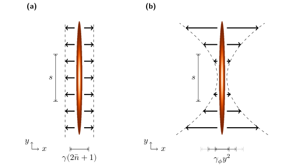
Before considering the combined effects of damping and dephasing however, we remark on the differences between these effects. They are most easily compared if the relevant equations of motion for the Wigner function are expressed in the same coordinate systems. We therefore rewrite the equation for damping (4.2) in polar coordinates, yielding (see also Appendix B)

	$\displaystyle\partial_{t}W(r,\phi,t)=$	$\displaystyle\frac{\gamma}{4}\left(\bar{n}+\frac{1}{2}\right)\underbrace{\left(\partial_{r}^{2}+\frac{1}{r}\partial_{r}+\frac{1}{r^{2}}\partial_{\phi}^{2}\right)}_{\nabla^{2}}W(r,\phi,t)$		(4.49)
		$\displaystyle+\frac{\gamma}{2}r\partial_{r}W(r,\phi,t)+\gamma W(r,\phi,t).$		(4.49)

Dephasing and damping both describe a diffusive processes which can be seen from the presence of second order derivatives on the right hand side. The dephasing equation however contains no derivatives with respect to the radial coordinate $r$ . This means that dephasing, in contrast to damping, only causes a flow of the Wigner density in the angular direction. For this reason, there exist states for which the Wigner function remains negative under any amount of evolution under dephasing.⁸⁸ 8 The number states $|n\rangle$ are a trivial example since they remain constant under dephasing. This is easily concluded either from the operator formalism (see (1.62)) or by substitution of (1.104) into (4.37). No such states exist for damping, since its effect is always decay toward the steady state solution thermal state (see Section 4.1.1).

It is also fruitful to note the difference between the terms causing angular diffusion. Angular diffusion is caused by the differential operator $\partial_{\phi}^{2}$ . In the dephasing equation (4.37) it has the constant coefficient $\gamma_{\phi}/2$ . In the damping equation the $\partial_{\phi}^{2}$ -term has the coefficient $\gamma\left(2\bar{n}+1\right)/8r^{2}$ . As noted in Section 4.2.1, the operator $\partial_{\phi}^{2}$ contains an implicit scaling of $r^{2}$ . This means that the diffusive effect of damping is constant everywhere in phase space (the drift towards the origin is not however). For the same reason, the diffusive effect of dephasing is proportional to $y^{2}$ and therefore vanishes toward the origin. This is illustrated in Figure 4.11. In the context of negativity, this means that negative regions closer to the origin are relatively more vulnerable to damping⁹⁹ 9 This view is consistent with the main result of Section 4.1, where it was shown that an increase in squeezing (which generally moves features of the Wigner function farther from the origin) reduces the adverse effect of damping. whereas negative regions far from the origin are relatively more vulnerable to dephasing.

This complementary character of dephasing and damping is clearly visible when comparing the evolution of the Wigner function. Under damping (Figure 4.4), the diffusive effect appears homogeneous throughout phase space. It appears to be the case that the regions which would have been at the center of negativity for the undamped oscillator maintain their negativity the longest under damping. In contrast, the diffusive effect of dephasing (see Figure 4.9) is clearly stronger further from the origin. The result is that the negative regions become concentrated close to the origin.

This may offer an explanation for why the large squeezing approximation is more effective for damping than dephasing (as observed in Section 4.2.2): The decay of negativity under dephasing happens only through angular diffusion. For positive and negative regions close to the origin to mix thus eliminating the negativity requires diffusion over an angle which is a appreciable fraction of $\pi$ . In the corresponding time, the diffusion farther from the origin, which is described by the same angle, will have caused a significant flow of Wigner density away from the $y$ -axis and toward the $x$ -axis causing a deterioration in the large squeezing approximation from considerations similar to those of Section 3.4.10.

4.3.2 Equation of Motion

We are now ready to construct the general equation of motion for the combined effects of dephasing and damping. The relevant master equation is obtained by including all terms of (1.60) and inserting the Kerr Hamiltonian (3.2) as $\hat{H}$ :

\dot{\hat{\rho}}=-ig\left[\hat{a}^{\dagger}\hat{a}^{\dagger}\hat{a}\hat{a},\hat{\rho}\right]+\gamma\left(\bar{n}+1\right)\mathcal{D}[\hat{a}]\hat{\rho}+\gamma\bar{n}\mathcal{D}[\hat{a}^{\dagger}]\hat{\rho}+\gamma_{\phi}\mathcal{D}[\hat{n}]\hat{\rho}.

(4.50)

We can derive the corresponding equation of motion for the Wigner function simply by combining (4.26) and (4.39) to obtain

\partial_{t}W(x,y,t)=\begin{aligned} &2g\left(x^{2}+y^{2}-1\right)\left(-y\partial_{x}+x\partial_{y}\right)W(x,y,t)\\ &-\frac{g}{8}\left(-y\partial_{x}+x\partial_{y}\right)\left(\partial_{x}^{2}+\partial_{y}^{2}\right)W(x,y,t)\\ &+\frac{\gamma}{4}\left(\bar{n}+\frac{1}{2}\right)\left(\partial_{x}^{2}+\partial_{y}^{2}\right)W(x,y,t)\\ &+\frac{\gamma}{2}\partial_{x}\left(xW(x,y,t)\right)+\frac{\gamma}{2}\partial_{y}\left(yW(x,y,t)\right)\\ &+\frac{\gamma_{\phi}}{2}\left(-y\partial_{x}+x\partial_{y}\right)\left(-y\partial_{x}+x\partial_{y}\right)W(x,y,t).\end{aligned}

(4.51)

The effects of the individual terms have already been described; see the previous section as well as Sections 3.2.3, 4.1 and 4.2.

4.3.3 Rescaled Coordinates and Large Squeezing Approximation

We introduce once again rescaled coordinates $(\tilde{x},\tilde{y})$ as given in (3.56) with corresponding differential operators as given in (3.59). The initial state is now given by (3.57) while (4.51) is transformed to

\partial_{t}\tilde{W}(\tilde{x},\tilde{y},t)=\begin{aligned} &2g\left(-\tilde{x}^{2}\tilde{y}\partial_{\tilde{x}}-s^{4}\tilde{y}^{3}\partial_{\tilde{x}}+\frac{1}{s^{4}}\tilde{x}^{3}\partial_{\tilde{y}}+\tilde{x}\tilde{y}^{2}\partial_{\tilde{y}}\right)\tilde{W}(\tilde{x},\tilde{y},t)\\ &-2g\left(-s^{2}\tilde{y}\partial_{\tilde{x}}+\frac{1}{s^{2}}\tilde{x}\partial_{\tilde{y}}\right)\tilde{W}(\tilde{x},\tilde{y},t)\\ &-\frac{g}{8}\left(-s^{4}\tilde{y}\partial_{\tilde{x}}^{3}+\frac{1}{s^{4}}\tilde{x}\partial_{\tilde{y}}^{3}+\tilde{x}\partial_{\tilde{y}}\partial_{\tilde{x}}^{2}-\tilde{y}\partial_{\tilde{x}}\partial_{\tilde{y}}^{2}\right)\tilde{W}(\tilde{x},\tilde{y},t)\\ &+\frac{\gamma s^{2}}{4}\left(\bar{n}+\frac{1}{2}\right)\partial_{\tilde{x}}^{2}\tilde{W}(\tilde{x},\tilde{y},t)+\frac{\gamma}{4s^{2}}\left(\bar{n}+\frac{1}{2}\right)\partial_{\tilde{y}}^{2}\tilde{W}(\tilde{x},\tilde{y},t)\\ &+\frac{\gamma}{2}\partial_{\tilde{x}}\left(\tilde{x}\tilde{W}(\tilde{x},\tilde{y},t)\right)+\frac{\gamma}{2}\partial_{\tilde{y}}\left(\tilde{y}\tilde{W}(\tilde{x},\tilde{y},t)\right).\\ &+\frac{\gamma_{\phi}}{2}\left(s^{4}\tilde{y}^{2}\partial_{\tilde{x}}^{2}+s^{-4}\tilde{x}^{2}\partial_{\tilde{y}}^{2}-2\tilde{x}\tilde{y}\partial_{\tilde{x}}\partial_{\tilde{y}}-\tilde{x}\partial_{\tilde{x}}-\tilde{y}\partial_{\tilde{y}}\right)\tilde{W}(\tilde{x},\tilde{y},t).\end{aligned}

(4.52)

We extract the most significant terms in the limit of large squeezing:

\partial_{t}\tilde{W}(\tilde{x},\tilde{y},t)=\begin{aligned} &-2gs^{4}\tilde{y}^{3}\partial_{\tilde{x}}\tilde{W}(\tilde{x},\tilde{y},t)+\frac{g}{8}s^{4}\tilde{y}\partial_{\tilde{x}}^{3}\tilde{W}(\tilde{x},\tilde{y},t)\\ &+\frac{\gamma s^{2}}{4}\left(\bar{n}+\frac{1}{2}\right)\partial_{\tilde{x}}^{2}\tilde{W}(\tilde{x},\tilde{y},t)+\frac{\gamma_{\phi}}{2}s^{4}\tilde{y}^{2}\partial_{\tilde{x}}^{2}\tilde{W}(\tilde{x},\tilde{y},t).\end{aligned}

(4.53)

The right hand side above is the sum of the right hand sides of (4.29) and (4.41). This again reduces the problem to a two-dimensional one. Thus define the function $\tilde{u}_{\tilde{y}}(\mu,\tilde{\tau})$ by

\tilde{W}(\tilde{x},\tilde{y},t)=\tilde{u}_{\tilde{y}}(\tilde{x}-2gs^{4}\tilde{y}^{3}t,gs^{4}\tilde{y}t/8).

(4.54)

From (4.53), the equation of motion for $u_{\tilde{y}}(\mu,\tilde{\tau})$ is given by

	$\partial_{\tilde{\tau}}\tilde{u}_{\tilde{y}}(\mu,\tilde{\tau})=\partial_{\mu}^{3}\tilde{u}_{\tilde{y}}(\mu,\tilde{\tau})+\beta_{\tilde{y}}\partial_{\mu}^{2}\tilde{u}_{\tilde{y}}(\mu,\tilde{\tau})$	(4.55a)
with
	$\beta_{\tilde{y}}=\left(\frac{\gamma(2\bar{n}+1)}{gs^{2}\tilde{y}}+\frac{4\gamma_{\phi}\tilde{y}}{g}\right).$	(4.55b)

(4.55) describes a third-order dispersive process with diffusion. The strength of the diffusion varies with $\tilde{y}$ and is described by $\beta_{\tilde{y}}$ . $\beta_{\tilde{y}}$ is a clear expression of the differences between damping and dephasing discussed in Section 4.3.1.¹⁰¹⁰ 10 On the $\tilde{y}$ -axis, the diffusion arising from damping is homogeneous throughout phase space whereas the diffusion from dephasing increases with $|\tilde{y}|^{2}$ . The damping contribution to $\beta_{\tilde{y}}$ in (4.55b) appears to vary in proportion to $\tilde{y}^{-1}$ , however this is because (4.55a) is expressed in terms of the rescaled time $\tilde{\tau}$ which carries an implicit factor of $\tilde{y}$ (see (4.54)). Additionally, increasing squeezing reduces the effects of damping due to the factor of $s^{2}$ in the denominator. This is in contrast to the dephasing term of $\beta_{\tilde{y}}$ which is invariant with respect to the squeezing $s$ .

One may solve for $\tilde{u}_{\tilde{y}}$ using a Fourier series as done previously. The solution for $\tilde{W}(\tilde{x},\tilde{y},t)$ is then obtained from this solution and (4.54) as


	$\displaystyle\tilde{W}(\tilde{x},\tilde{y},t)$	$\displaystyle=\frac{1}{\sqrt{2\pi}}\int_{-\infty}^{\infty}dk\,h_{\tilde{y}}(k)\,e^{i(k\tilde{x}-2kgts^{4}\tilde{y}^{3}-gts^{4}k^{3}\tilde{y}/8)}e^{-\gamma(2\bar{n}+1)s^{2}t/8}e^{-\gamma_{\phi}s^{4}\tilde{y}^{2}t/2}$	(4.56a)
where the Fourier transform of the initial state is given by
	$h_{\tilde{y}}(k)=\frac{1}{\sqrt{2\pi}}\int_{-\infty}^{\infty}d\tilde{x}\,\tilde{W}(\tilde{x},\tilde{y},0)\,e^{-ik\tilde{x}}.$		(4.56b)

This reveals the scaling of diffusion as $\tilde{y}^{2}$ and unit for dephasing and damping respectively.

4.3.4 Maximum Negative Volume and Peak

(a) Maximum negative volume

\max_{t}N_{\mathrm{vol}}

(b) Maximum negative peak

\max_{t}N_{\mathrm{peak}}

Figure 4.13: Maximum negativity contours for combined decoherence. Contours of maximum negative volume

\max_{t}N_{\mathrm{vol}}

and maximum negative peak

\max_{t}N_{\mathrm{peak}}

as a function of decoherence rates. The effective damping rate

\gamma(2\bar{n}+1)s^{2}

was set with

\bar{n}=1000

. Figure 4.12 shows the source of the contour for

r_{0}=1.75

. For low dephasing, the maximum negativity as a function of effective damping rate appear independent of the squeezing

s

. For larger dephasing rates, the negativity increases with

s

. The data is discussed in Section 4.3.4. Thick dotted lines (

r_{0}\to\infty

) show the contours obtained from (4.56). The contour at

10^{-4.5}

is not shown for

r_{0}=1.5

To quantify the interplay between damping and dephasing, we study the maximum negative volume and peak for various values of the parameters $r_{0}$ , $\gamma_{\phi}$ and $\gamma(2\bar{n}+1)$ . Figure 4.12 shows the negativity in the case $r_{0}=1.75$ . The parameters that take values of frequency are normalized to the value of $g$ . It is seen that an increase in either $\gamma_{\phi}/g$ or $\gamma(2\bar{n}+1)/gs^{2}$ always cause a decrease in the maximum negativity irrespective of the value of the other decoherence parameter. We also note that the adverse effects on the maximum negativity combine in a super-linear way and that one can therefore not describe the maximum negative volume as the sum of the two effects, i.e. one cannot define functions $f_{\gamma}$ and $f_{\gamma_{\phi}}$ to make the following an equality:

\max_{t}N_{\mathrm{vol}}\neq f_{\gamma}\left(\gamma(2\bar{n}+1)\right)+f_{\gamma_{\phi}}(\gamma_{\phi}),

(4.57)

as equality in (4.57) would have manifested itself as straight line contours in Figure 4.12. The same conclusion is reached for $\max_{t}N_{\mathrm{peak}}$ .

To investigate the dependence on the squeezing $s$ , we superimpose the contours of the maximum negativity with $r_{0}$ taking the values $1$ , $1.25$ , $1.5$ and $1.75$ (of which Figure 4.12 shows the case $r_{0}=1.75$ ) in Figure 4.13. This indicates the regions where the large squeezing approximation of Section 4.3.3 is valid. We see that the contours assume common values for larger values of $r_{0}$ and effective damping $\gamma(2\bar{n}+1)/gs^{2}$ as expected. We also show the contours obtained from the Fourier transformed solution (4.56) to the equation after the large squeezing approximation. These match well with the contours of $r_{0}=1.75$ suggesting that it may be possible to find an asymptotic behavior for the entire graph given sufficient squeezing.

We also note that the contours appear to diverge as $\gamma_{\phi}/g$ is increased and $\gamma(2\bar{n}+1)/gs^{2}$ decreased. This means that a large squeezing is required for the large squeezing approximation to work with dephasing than with damping. This is a similar observation to that made for the maximum negative volume as a function of $\gamma_{\phi}/g$ in Figure 4.10. Assuming that increased $\gamma_{\phi}/g$ can never lead to an increase in negativity (which has not been proven here, but seems like a reasonable assumption given that dephasing can be described as angular diffusion and commutes with both effects of the unitary term and damping, see Appendix C), the conclusion is that an increase in squeezing can compensate for a small ratio $\gamma(2\bar{n}+1)/g$ when measuring the maximum negativity without any adverse effects even for nonzero $\gamma_{\phi}/g$ .

4.4 Summary of Scalings for the Squeezed Vacuum State

We end the chapter by summarizing the discovered scalings for the evolution of negativity for the squeezed vacuum state $|\xi=r_{0}\rangle$ . These are listed in Table 4.2. In Chapter 3 we considered the unitary dynamics of the Kerr oscillator. For large squeezing only the most significant terms were kept, rendering the approximated equation of motion in a form in which $s$ and the Kerr coefficient $g$ entered only in the combination $gs^{4}$ (displayed in Table 4.2). Since the frequency $gs^{4}$ is now the only parameter, the time $t$ was be rescaled to $gts^{4}$ (also displayed in Table 4.2) such that both the initial state and the equation of motion are free of parameters. In this chapter, the appropriate scaling of time was then established for the cases of isolated damping or dephasing (significant terms in the equation of motion as well as appropriate scalings of time listed in Table 4.2). The respective scaled times were found to describe the decay of negativity as a result of both isolated damping and dephasing. The case of simultaneous Kerr evolution and high temperature damping of effective rate $\gamma(2\bar{n}+1)$ were investigated and the maximum negativity was found to be well described by the ratio of the scaled times $gs^{2}/\gamma(2\bar{n}+1)$ . In case of the dephasing however Kerr oscillator, the scaled time did not by itself account for the relation between maximum negativity, squeezing and dephasing rate.

Effect Scaled time Significant terms Relevant sections and figures Kerr oscillator $tgs^{4}$ $gs^{4}\left(-2\tilde{y}^{3}\partial_{\tilde{x}}+\frac{1}{8}\tilde{y}\partial_{\tilde{x}}^{3}\right)\tilde{W}$ Sections 3.4.3–3.4.11. from (3.72) from (3.60) Figures 3.11 and 3.14. Damping $t\gamma(2\bar{n}+1)s^{2}$ $\frac{1}{8}\gamma s^{2}\left(2\bar{n}+1\right)\partial_{\tilde{x}}^{2}\tilde{W}$ Sections 4.1.2 and 4.1.3. from (4.20) from (4.17) Figures 4.3 and 4.6. Dephasing $t\gamma_{\phi}s^{4}$ $\frac{1}{2}\gamma_{\phi}s^{4}\tilde{y}^{2}\partial_{\tilde{x}}^{2}\tilde{W}$ Sections 4.2.1 and 4.2.2. from (4.43) from (4.40) Figures 4.8 and 4.10.

Table 4.2: Summary of scaling relations for squeezed vacuum. Table summarizing the main results for the short time evolution of the squeezed vacuum state. The unitary Kerr evolution as well as the decoherence effects of damping and dephasing are listed. When plotting the negativity for short times as a function of the scaled time, the graphs exhibit asymptotic behavior as

r_{0}

is increased. We can understand this behavior by rescaling the Wigner function as described in Section 3.4.7 such that the most significant terms in its equation of motion (also tabulated) will appear with the squeezing explicit. The final column references passages of particular relevance from this thesis.

Conclusion

In this thesis, we studied the evolution of a squeezed vacuum state of the Kerr oscillator. We focus specifically on the formation of negativity of the Wigner function. To gain a better understanding of the system, we studied first the unitary dynamics. We explored the analytical operator solution which describes a periodic evolution in the state. Motivated by the damping of current experimental systems, we then studied the evolution of the squeezed vacuum state over short time intervals. Various tools were employed to gain a geometrical understanding of the state evolution for short times. We then used the Fokker-Planck-like equation for the evolution of the Wigner function to develop a solution in the limit of large negativity. This solution was then used to show that the nonlinearity $g$ scales as $ge^{4r_{0}}$ where $r_{0}$ denotes the squeezing parameter. We also considered the open system of a damped and dephasing Kerr oscillator. Using the large-squeezing solution for the unitary case, it was found that the effective ratio between nonlinearity and damping was improved with squeezing by a factor of $e^{2r_{0}}$ . Combining the effects of dephasing and damping, it was shown that the enhancement of the effective ratio between nonlinearity and damping through squeezing does not have an exacerbating effect on the decoherence arising from dephasing. Table 4.2 lists relevant results for scaling.

Several avenues of further exploration have presented themselves during this work. Building directly upon the results here, it appears plausible from Chapter 3 that the results of Chapter 4 can be straightforwardly extended to include squeezed thermal states. On a more technical level, work could be done to quantify the accuracy of the large squeezing approximation for any Gaussian state beyond what has been done here. Of course, the ability to strongly squeeze the vacuum state is essential to the direct applicability of the results presented here and one should thus survey the experimental results for this before proceeding. Optical squeezing of up to $15$ dB has been observed experimentally [65].

It has also been suggested to apply Kerr evolution to a coherent initial state to form negativity in the Wigner function [2]. This is experimentally attractive since coherent states are far easier to prepare experimentally. Since the negativity for the coherent state only forms near the coherent displacement amplitude in phase space however (cf. Figure 3.22), the coherent state may be more vulnerable to the effects of dephasing. This suggests a comparison between the evolution in negativity for coherent and squeezed states. The methods demonstrated for the squeezed state in this thesis may find use in developing a similar understanding for the formation of negativity in the evolution of a coherent state. It may also be possible to show that limited squeezing of a coherent state will amplify the nonlinear effects of the Kerr oscillator.

Experimental measurement of Wigner function negativity requires the development of mechanical state tomography [66]. It may be shown that squeezing a state does not hamper the ability to reconstruct the state Wigner function from measurements of its marginal distributions [67]. As part of this, the quadrature squeezing could also be introduced as simultaneous with the Kerr evolution rather than as a prior step. One could also explore alternate effects such as the use of feedback to enhance the nonlinear effects or stabilize a state with negative Wigner function [42].

In summary, we have shown that one may compensate for a weak nonlinearity through squeezing. This opens the door to witness a negative Wigner function in a macroscopic mechanical system even if nonlinearity is a scarce resource, provided that the ability to squeeze the system state significantly exists. While the work in this thesis has been motivated by nanomechanical systems, most of it is general to any quantum system described by a Kerr oscillator where damping dominates and which allows for quadrature squeezing.

References

[1] E. Wigner “On the Quantum Correction For Thermodynamic Equilibrium” In Physical Review 40.5, 1932, pp. 749–759
[2] Magdalena Stobińska, G.. Milburn and Krzysztof Wódkiewicz “Wigner Function Evolution of Quantum States in the Presence of Self-Kerr Interaction” In Physical Review A 78.1, 2008, pp. 013810 DOI: 10.1103/PhysRevA.78.013810
[3] G.. Milburn and C.. Holmes “Dissipative Quantum and Classical Liouville Mechanics of the Anharmonic Oscillator” In Physical Review Letters 56.21, 1986, pp. 2237–2240 DOI: 10.1103/PhysRevLett.56.2237
[4] Y. Tsaturyan, A. Barg, E.. Polzik and A. Schliesser “Ultracoherent Nanomechanical Resonators via Soft Clamping and Dissipation Dilution” In Nature Nanotechnology 12.8, 2017, pp. 776–783 DOI: 10.1038/nnano.2017.101
[5] Jasper Chan et al. “Laser Cooling of a Nanomechanical Oscillator into Its Quantum Ground State” In Nature 478.7367, 2011, pp. 89–92 DOI: 10.1038/nature10461
[6] E.. Wollman et al. “Quantum Squeezing of Motion in a Mechanical Resonator” In Science 349.6251, 2015, pp. 952–955 DOI: 10.1126/science.aac5138
[7] B. Yurke and D. Stoler “Generating Quantum Mechanical Superpositions of Macroscopically Distinguishable States via Amplitude Dispersion” In Physical Review Letters 57.1, 1986, pp. 13–16
[8] Seth Lloyd and Samuel. Braunstein “Quantum Computation over Continuous Variables” In Physical Review Letters 82.8, 1999, pp. 1784–1787 DOI: 10.1103/PhysRevLett.82.1784
[9] Letizia Catalini “Mechanical Nonlinearities” internal report, 2018
[10] Massimiliano Rossi et al. “Measurement-Based Quantum Control of Mechanical Motion” In Nature 563, 2018, pp. 53–58
[11] Rajan Singh et al. “Giant Tunable Mechanical Nonlinearity in Graphene-Silicon Nitride Hybrid Resonator”, 2019 arXiv:1904.01613
[12] M.. Woolley, G.. Milburn and Carlton. Caves “Nonlinear Quantum Metrology Using Coupled Nanomechanical Resonators” In New Journal of Physics 10.12, 2008, pp. 125018 DOI: 10.1088/1367-2630/10/12/125018
[13] Kurt Jacobs and Andrew. Landahl “Engineering Giant Nonlinearities in Quantum Nanosystems” In Physical Review Letters 103.6, 2009, pp. 067201
[14] Christopher Gerry and Peter Knight “Introductory Quantum Optics” Cambridge University Press, 2004
[15] J.. Sakurai and Jim Napolitano “Modern Quantum Mechanics” Addison-Wesley, 2011
[16] H.. Wiseman and G.. Milburn “Quantum Measurement and Control” Cambridge University Press, 2010
[17] Franz Schwabl “Statistical Mechanics” Springer, 2006
[18] D.. Walls and Gerard. Milburn “Quantum Optics” Springer, 2008
[19] Miguel Orszag “Quantum Optics: Including Noise Reduction, Trapped Ions, Quantum Trajectories, and Decoherence” Springer, 2016
[20] D.. Wilson et al. “Measurement-Based Control of a Mechanical Oscillator at Its Thermal Decoherence Rate” In Nature 524, 2015, pp. 325
[21] K. Hornberger “Introduction to Decoherence Theory” In Entanglement and Decoherence 768 Springer, 2009, pp. 221–276
[22] K.. Cahill and R.. Glauber “Density Operators and Quasiprobability Distributions” In Physical Review 177.5, 1969, pp. 1882–1902
[23] Marlan. Scully and M. Zubairy “Quantum Optics” Cambridge University Press, 1997
[24] Warwick. Bowen and Gerard Milburn “Quantum Optomechanics” CRC Press, 2015
[25] J.. Moyal “Quantum Mechanics as a Statistical Theory” In Mathematical Proceedings of the Cambridge Philosophical Society 45.1, 1949, pp. 99–124
[26] Thomas Curtright, David Fairlie and Cosmas Zachos “A Concise Treatise on Quantum Mechanics in Phase Space” World Scientific, 2014
[27] Alessandro Ferraro, Stefano Olivares and Matteo.. Paris “Gaussian States in Quantum Information” Bibliopolis, 2005
[28] R.. Hudson “When Is the Wigner Quasi-Probability Density Non-Negative?” In Reports on Mathematical Physics 6.2, 1974, pp. 249–252
[29] Anatole Kenfack and Karol Życzkowski “Negativity of the Wigner Function as an Indicator of Non-Classicality” In Journal of Optics B: Quantum and Semiclassical Optics 6.10, 2004, pp. 396–404
[30] Itamar Katz, Ron Lifshitz, Alex Retzker and Raphael Straub “Classical to Quantum Transition of a Driven Nonlinear Nanomechanical Resonator” In New Journal of Physics 10.12, 2008, pp. 125023
[31] J.. Corney and M.. Olsen “Non-Gaussian Pure States and Positive Wigner Functions” In Physical Review A 91.2, 2015, pp. 023824
[32] Salman Habib et al. “Quantum-Classical Transition in Nonlinear Dynamical Systems” In Physical Review Letters 88.4, 2002, pp. 040402
[33] Maxime Oliva and Ole Steuernagel “Quantum Kerr Oscillators’ Evolution in Phase Space: Wigner Current, Symmetries, Shear Suppression, and Special States” In Physical Review A 99.3, 2019, pp. 032104
[34] Heiko Bauke and Noya Itzhak “Visualizing Quantum Mechanics in Phase Space”, 2011 arXiv:1101.2683
[35] Oscar. Friedman and Miles. Blencowe “The Wigner Flow for Open Quantum Systems”, 2017 arXiv:1703.04844
[36] D. Leibfried et al. “Experimental Determination of the Motional Quantum State of a Trapped Atom” In Physical Review Letters 77.21, 1996, pp. 4281–4285
[37] Antoine Royer “Wigner Function as the Expectation Value of a Parity Operator” In Physical Review A 15.2, 1977, pp. 449–450
[38] William. Case “Wigner Functions and Weyl Transforms for Pedestrians” In American Journal of Physics 76.10, 2008, pp. 937–946
[39] George Arfken, Hans Weber and Frank Harris “Mathematical Methods for Physicists” Academic Press, 2012
[40] Cosmas. Zachos, David. Fairlie and Thomas. Curtright “Quantum Mechanics in Phase Space: An Overview with Selected Papers” World Scientific Publishing Company Incorporated, 2005
[41] Ievgen. Arkhipov, Artur Barasiński and Jiří Svozilík “Negativity Volume of the Generalized Wigner Function as an Entanglement Witness for Hybrid Bipartite States” In Scientific Reports 8.1, 2018, pp. 1–11
[42] Martin Koppenhöfer, Christoph Bruder and Niels Lörch “Heralded Dissipative Preparation of Nonclassical States in a Kerr Oscillator”, 2019 arXiv:1906.05126
[43] J.. Johansson, P.. Nation and Franco Nori “QuTiP: An Open-Source Python Framework for the Dynamics of Open Quantum Systems” In Computer Physics Communications 183.8, 2012, pp. 1760–1772
[44] J.. Johansson, P.. Nation and Franco Nori “QuTiP 2: A Python Framework for the Dynamics of Open Quantum Systems” In Computer Physics Communications 184.4, 2013, pp. 1234–1240
[45] Peter. Brown, Alan. Hindmarsh and George. Byrne “ZVODE: Variable-Coefficient Ordinary Differential Equation Solver, C with Fixed-Leading-Coefficient Implementation.” URL: www.netlib.org/ode/zvode.f
[46] M.. Bartlett and J.. Moyal “The exact transition probabilities of quantum-mechanical oscillators calculated by the phase-space method” In Mathematical Proceedings of the Cambridge Philosophical Society 45.4 Cambridge University Press, 1949, pp. 545–553 DOI: 10.1017/S030500410002524X
[47] M.. Levenson, R.. Shelby and S.. Perlmutter “Squeezing of Classical Noise by Nondegenerate Four-Wave Mixing in an Optical Fiber” In Optics Letters 10.10, 1985, pp. 514–516 DOI: 10.1364/OL.10.000514
[48] J.. Home et al. “Normal Modes of Trapped Ions in the Presence of Anharmonic Trap Potentials” In New Journal of Physics 13.7, 2011, pp. 073026
[49] Markus Aspelmeyer, Tobias. Kippenberg and Florian Marquardt “Cavity Optomechanics” In Reviews of Modern Physics 86.4, 2014, pp. 1391–1452
[50] Silvan Schmid, Luis Villanueva and Michael Roukes “Fundamentals of Nanomechanical Resonators” Springer International Publishing, 2016
[51] E. Babourina-Brooks, A. Doherty and G.. Milburn “Quantum Noise in a Nanomechanical Duffing Resonator” In New Journal of Physics 10.10, 2008, pp. 105020
[52] P. Bocchieri and A. Loinger “Quantum Recurrence Theorem” In Physical Review 107.2, 1957, pp. 337–338
[53] Maxime Oliva and Ole Steuernagel “Dynamic Shear Suppression in Quantum Phase Space” In Physical Review Letters 122.2, 2019, pp. 020401
[54] J.. Huber et al. “Detecting Squeezing from the Fluctuation Spectrum of a Driven Nanomechanical Mode”, 2019 arXiv: http://arxiv.org/abs/1903.07601
[55] Alfredo Villanueva “On Linearized Korteweg-de Vries Equations” In Journal of Mathematics Research 4.1, 2012, pp. 2
[56] Peter. Olver and Efstratios Tsatis “Points of Constancy of the Periodic Linearized Korteweg–deVries Equation” In Proceedings of the Royal Society A: Mathematical, Physical and Engineering Sciences 474.2217, 2018, pp. 20180160
[57] Peter. Olver “Introduction to Partial Differential Equations” Springer, 2013
[58] Andrew. White et al. “Kerr Noise Reduction and Squeezing” In Journal of Optics B: Quantum and Semiclassical Optics 2.4, 2000, pp. 553–561
[59] C.. Gardiner “Handbook in Stochastic Processes Methods for Physics, Chemistry and the Natural Sciences” Springer, 1985
[60] Ming Wang and G.. Uhlenbeck “On the Theory of the Brownian Motion II” In Reviews of Modern Physics 17.2-3, 1945, pp. 323–342
[61] H.. Korsch, C. Müller and H. Wiescher “On the Zeros of the Husimi Distribution” In Journal of Physics A: Mathematical and General 30.20, 1997, pp. L677–L684
[62] Ching Lee “Measure of the Nonclassicality of Nonclassical States” In Physical Review A 44.5, 1991, pp. R2775–R2778
[63] Ching Lee “Moments of P Functions and Nonclassical Depths of Quantum States” In Physical Review A 45.9, 1992, pp. 6586–6595
[64] M.. Marchiolli, V.. Bagnato, Y. Guimarães and B. Baseia “Nonclassical Depth of the Phase State” In Physics Letters A 279.5, 2001, pp. 294–304
[65] Henning Vahlbruch, Moritz Mehmet, Karsten Danzmann and Roman Schnabel “Detection of 15 dB Squeezed States of Light and Their Application for the Absolute Calibration of Photoelectric Quantum Efficiency” In Physical Review Letters 117.11, 2016, pp. 110801 DOI: 10.1103/PhysRevLett.117.110801
[66] Michael. Vanner, Igor Pikovski and M.. Kim “Towards Optomechanical Quantum State Reconstruction of Mechanical Motion” In Annalen der Physik 527.1-2, 2015, pp. 15–26 DOI: 10.1002/andp.201400124
[67] Luca Fresta, Johannes Borregaard and Anders. Sørensen “Elementary Test for Nonclassicality Based on Measurements of Position and Momentum” In Physical Review A 92.6, 2015, pp. 062111
[68] Aaron Meurer et al. “SymPy: Symbolic Computing in Python” In PeerJ Computer Science 3, 2017, pp. e103
[69] G.. D’Ariano, M. Fortunato and P. Tombesi “Time Evolution of an Anharmonic Oscillator Interacting with a Squeezed Bath” In Quantum and Semiclassical Optics: Journal of the European Optical Society Part B 7.6, 1995, pp. 933–942 DOI: 10.1088/1355-5111/7/6/002

List of Figures

List of Tables

Appendix A Interaction Picture and Rotating Wave Approximation

Consider the Hamiltonian

\hat{H}=\frac{\hat{p}^{2}}{2m}+\frac{1}{2}m\omega^{2}\hat{q}^{2}+\frac{\beta}{4}\hat{q}^{4}.

(A.1)

This describes the quantum mechanical Duffing oscillator [51] with mass $m$ and base frequency $\omega$ . $\beta$ is the Duffing parameter and has dimensions of mass times the square of ratio of angular frequency to length, i.e.

[\beta]=\frac{(\text{energy})}{(\text{length})^{4}}=(\text{mass})\cdot\frac{(\text{angular frequency})^{2}}{(\text{length})^{2}}.

(A.2)

The Duffing oscillator describes an oscillator where the (angular) frequency is dependent on the displacement. $\sqrt{\beta}$ relates the change in displacement to the corresponding change in (angular) frequency. With the conventions used here, $\beta$ is additionally scaled with the mass of the oscillator.

From (A.1), we may derive Langevin equations for the system operators $\hat{q}$ and $\hat{p}$ to be

\dot{\hat{q}}=\frac{\hat{p}}{m}

(A.3)

and

\dot{\hat{p}}=-m\omega^{2}\hat{q}-m\gamma\dot{\hat{q}}-\beta\hat{q}^{3}.

(A.4)

Equations (A.3) and (A.4), or equivalently

\ddot{\hat{q}}=-\omega^{2}\hat{q}-\gamma\dot{\hat{q}}-\frac{\beta}{m}\hat{q}^{3},

(A.5)

are often used to introduce the dynamics of the Duffing oscillator in place of (A.1).

(A.1) also allows us to write the Hamiltonian as

\hat{H}=\hbar\omega\left(\hat{a}^{\dagger}\hat{a}+\frac{1}{2}\right)+\frac{\hbar^{2}\beta}{16m^{2}\omega^{2}}\left(\hat{a}+\hat{a}^{\dagger}\right)^{4}.

(A.6)

We wish to express $\hat{H}$ in the interaction picture with

\hat{H}_{0}=\hbar\omega_{0}\hat{a}^{\dagger}\hat{a}

(A.7)

as the base Hamiltonian. We can then transition to the interaction picture by simply substituting [15]:

	$\displaystyle\hat{a}$	$\displaystyle\to\hat{a}_{I}=e^{i\hat{H}_{0}t}\hat{a}e^{-i\hat{H}_{0}t}=\hat{a}e^{-i\omega_{0}t}\,,$		(A.8)
	$\displaystyle\hat{a}^{\dagger}$	$\displaystyle\to\hat{a}_{I}^{\dagger}=e^{i\hat{H}_{0}t}\hat{a}^{\dagger}e^{-i\hat{H}_{0}t}=\hat{a}^{\dagger}e^{i\omega_{0}t}\,.$		(A.9)

Substitution yields the interaction Hamiltonian

\displaystyle\hat{H}_{I}

\displaystyle=\begin{aligned} &\frac{3\hbar^{2}\beta}{8m^{2}\omega_{0}^{2}}\left(\hat{a}^{\dagger}\hat{a}^{\dagger}\hat{a}\hat{a}+2\hat{a}^{\dagger}\hat{a}+\frac{1}{2}\right)+\frac{\hbar^{2}\beta}{8m^{2}\omega_{0}^{2}}\left[\left(2\hat{a}^{\dagger}\hat{a}^{3}+3\hat{a}^{2}\right)e^{-2i\omega_{0}t}+\mathrm{h.c.}\right]\\ &+\frac{\hbar^{2}\beta}{16m^{2}\omega_{0}^{2}}\left(\hat{a}^{4}e^{-4i\omega_{0}t}+\mathrm{h.c.}\right)+\hbar(\omega-\omega_{0})\left(\hat{a}^{\dagger}\hat{a}\right).\end{aligned}

(A.10)

”h.c.” is a placeholder for the Hermitian conjugate of the other terms within its innermost containing parentheses. Setting $\omega_{0}=\omega$ , the base oscillator frequency is removed. Under the assumption of a relatively large base oscillator frequency $\omega$ ,

\omega\gg g,

the oscillating terms can be neglected and we are left with¹¹ 1 The coefficient of the term $\hat{a}^{\dagger}\hat{a}$ in (A.11) is arbitrary in the sense that it can be made to have any value by appropriate choice of the interaction picture frequency $\omega_{0}$ in (A.7). Choosing $\omega_{0}$ as the real root of the third degree polynomial $4m^{2}\omega_{0}^{2}(\omega-\omega_{0})+3\hbar^{2}\beta$ would cause the term to vanish. With the assumption (3.4) however, we may consider $\omega_{0}=\omega$ to be a root of the polynomial.

\hat{H}_{\mathrm{RWA}}=\frac{3\hbar^{2}\beta}{8m^{2}\omega^{2}}\left(\hat{a}^{\dagger}\hat{a}^{\dagger}\hat{a}\hat{a}+2\hat{a}^{\dagger}\hat{a}+\frac{1}{2}\right).

(A.11)

This is the rotating wave approximation (hence the change of subscript). To consolidate with the Hamiltonian central to this thesis:

\hat{H}=\hbar g\hat{a}^{\dagger}\hat{a}^{\dagger}\hat{a}\hat{a},

we identify

g=\frac{3\hbar\beta}{8m^{2}\omega^{2}}.

Appendix B Equations of Motion for the Wigner Function

A procedure for deriving equivalent c-number equations from the master equation is described in Section 1.13. We start from the master equation (1.60) and insert a general Hamiltonian containing a simple harmonic oscillator term, a Kerr nonlinearity term and parametric squeezing terms proportional to the respective coefficients $\omega$ , $g$ and $|\eta|$ :

\hat{H}=\hbar\omega\hat{a}^{\dagger}\hat{a}+\hbar g\hat{a}^{\dagger}\hat{a}^{\dagger}\hat{a}\hat{a}+i\hbar\left(\eta^{*}\hat{a}\hat{a}-\eta\hat{a}^{\dagger}\hat{a}^{\dagger}\right).

(B.1)

(B.1) is inserted into the general master equation, (1.60), to arrive at the master equation for the density matrix $\hat{\rho}$ :


$\displaystyle\dot{\hat{\rho}}$	$\displaystyle=-i\omega\left[\hat{a}^{\dagger}\hat{a},\hat{\rho}\right]-ig\left[\hat{a}^{\dagger}\hat{a}^{\dagger}\hat{a}\hat{a},\hat{\rho}\right]+\left[\eta^{*}\hat{a}\hat{a}-\eta\hat{a}^{\dagger}\hat{a}^{\dagger},\hat{\rho}\right]$	(B.2a)
	$\displaystyle\qquad+\gamma(\bar{n}+1)\mathcal{D}\left[\hat{a}\right]\hat{\rho}+\gamma\bar{n}\mathcal{D}\left[\hat{a}^{\dagger}\right]\hat{\rho}+\gamma_{\phi}\mathcal{D}\left[\hat{n}\right]\hat{\rho}.$

Equation (B.2) is the most general master equation we will need to consider in this thesis. Below, corresponding terms in the partial differential equation for the Wigner function are separately derived for each term in (B.2). Symbolic manipulations were performed with the help of the Python library SymPy [68].

The steps to move from the master equation to the corresponding partial differential equation for the Wigner function are described in Section 1.13. The procedure is briefly outlined here as well: First, the time derivative of the symmetrically ordered characteristic function¹¹ 1 The derivations in the following sections take us by the function $\chi(\lambda,\lambda^{*},t)=\left\langle\hat{D}(\lambda)\right\rangle$ . For consistency in expressions where it and expectation values of other operator quantities appear however, we shall keep it expressed simply as the expectation value of $\hat{D}(\lambda)$ . is written $\partial_{t}\chi(\lambda,\lambda^{*},t)=\mathrm{Tr}\left[\dot{\hat{\rho}}\hat{D}(\lambda)\right]$ . Replacing $\dot{\hat{\rho}}$ by its right hand side from (B.2a), one obtains the trace of a sum of several operators. The linearity of the trace can be used to consider the trace of each term separately instead. The argument of the trace in each term consists of the factors $\hat{\rho}$ and $\hat{D}(\lambda)$ with some number of interspersed ladder operators $\hat{a}$ and $\hat{a}^{\dagger}$ . Next, the cyclic property of the trace is employed to in turn apply each ladder operator to $\hat{D}(\lambda)$ from either left or right. The exhaustive list of possibilities is found in (1.97). Neither $\partial_{\lambda}$ , $\partial_{\lambda^{*}}$ , $\lambda$ or $\lambda^{*}$ are operator quantities, so moving them outside the trace allows each term to take the general form $\lambda^{m}\left(\lambda^{*}\right)^{n}\partial_{\lambda}^{p}\partial_{\lambda^{*}}^{q}\left\langle\hat{D}(\lambda)\right\rangle$ . The resulting expression is a partial differential equation in $\lambda$ , $\lambda^{*}$ and $t$ for $\left\langle\hat{D}(\lambda)\right\rangle$ . Finally, for each term in this differential equation, derive the corresponding term in the partial differential equation for the Wigner function by considering the complex Fourier transform from the symmetrically ordered characteristic function to the Wigner function. This correspondence is computed for the general term as given by (1.98).

B.0 Coordinate Systems

Before we catalogue the equations of motion arising from the effects studied in this thesis, we state the identities necessary for conversion from the coordinate $\alpha$ to Cartesian and polar coordinates.

Cartesian coordinates $(x,y)$ were defined by

	$\displaystyle\alpha$	$\displaystyle=x+iy,$
	$\displaystyle\alpha^{*}$	$\displaystyle=x+iy,$		(B.3)

with the inverse relations

	$\displaystyle x$	$\displaystyle=\mathrm{Re}\alpha=\frac{1}{2}(\alpha+\alpha^{*}),$		(1.85a)
	$\displaystyle y$	$\displaystyle=\mathrm{Im}\alpha=\frac{1}{2i}(\alpha-\alpha^{*}).$		(1.85b)

The differential operators $\partial_{\alpha}$ and $\partial_{\alpha^{*}}$ are then


$\displaystyle\partial_{\alpha}$	$\displaystyle=\left(\partial_{\alpha}x\right)\partial_{x}+\left(\partial_{\alpha}y\right)\partial_{y}=\frac{1}{2}\partial_{x}+\frac{1}{2i}\partial_{y},$	(B.4a)
$\displaystyle\partial_{\alpha^{*}}$	$\displaystyle=\left(\partial_{\alpha^{}}x\right)\partial_{x}+\left(\partial_{\alpha^{}}y\right)\partial_{y}=\frac{1}{2}\partial_{x}-\frac{1}{2i}\partial_{y}.$	(B.4b)

Polar coordinates were defined by

	$\displaystyle\alpha$	$\displaystyle=re^{i\phi}$
	$\displaystyle\alpha^{*}$	$\displaystyle=re^{-i\phi}$		(B.5)

with the inverse relations

	$\displaystyle r$	$\displaystyle=\|\alpha\|,$		(B.6)
	$\displaystyle\phi$	$\displaystyle=\arg\alpha.$		(B.7)

The differential operators $\partial_{\alpha}$ and $\partial_{\alpha^{*}}$ are then


$\displaystyle\partial_{\alpha}$	$\displaystyle=\left(\partial_{\alpha}r\right)\partial_{r}+\left(\partial_{\alpha}\phi\right)\partial_{\phi}=\frac{1}{2}e^{-i\phi}\partial_{r}+\frac{1}{2ir}e^{-i\phi}\partial_{\phi},$	(B.8a)
$\displaystyle\partial_{\alpha^{*}}$	$\displaystyle=\left(\partial_{\alpha^{}}r\right)\partial_{r}+\left(\partial_{\alpha^{}}\phi\right)\partial_{\phi}=\frac{1}{2}e^{i\phi}\partial_{r}-\frac{1}{2ir}e^{i\phi}\partial_{\phi}.$	(B.8b)

We also note the following direct relations between the Cartesian and polar coordinates. In particular, the Laplacian $\nabla^{2}$ is used in both Cartesian and polar coordinate systems where appropriate.


$\displaystyle r\partial_{r}$	$\displaystyle=x\partial_{x}+y\partial_{y},$	(B.9a)
$\displaystyle\partial_{\phi}$	$\displaystyle=-y\partial_{x}+x\partial_{y},$	(B.9b)
$\displaystyle\nabla^{2}$	$\displaystyle=\partial_{x}^{2}+\partial_{y}^{2}=\left(\partial_{r}^{2}+r^{-2}\partial_{\phi}^{2}+r^{-1}\partial_{r}\right),$	(B.9c)
$\displaystyle\partial_{\phi}^{2}$	$\displaystyle=y^{2}\partial_{x}^{2}+x^{2}\partial_{y}^{2}-2xy\partial_{x}\partial_{y}-x\partial_{x}-y\partial_{y}.$	(B.9d)

For reference, we also note that the divergence of a vector

\mathbf{v}=v_{x}\hat{\mathbf{x}}+v_{y}\hat{\mathbf{y}}=v_{r}\hat{\mathbf{r}}+v_{\phi}\bm{{\phi}}

(B.10)

is given by

\nabla\cdot\mathbf{v}=\partial_{x}v_{x}+\partial_{y}v_{y}=\frac{1}{r}\partial_{r}\left(rv_{r}\right)+\frac{1}{r}\partial_{\phi}v_{\phi}.

(B.11)

B.1 Harmonic Oscillator

The von Neumann equation for the simple harmonic oscillator takes the form

\dot{\hat{\rho}}=-i\omega\left[\hat{a}^{\dagger}\hat{a},\hat{\rho}\right].

(B.12)

This dynamics of the term are notable for commuting with all other dynamics of (B.2) except for parametric squeezing. Translating each term into an equation for the displacement operator yields the terms


$\displaystyle-i\omega\left\langle\hat{D}(\lambda)\hat{a}^{\dagger}\hat{a}\right\rangle$	$\displaystyle=-i\omega\left(-\frac{\lambda^{}}{2}+\partial_{\lambda}\right)\left(-\frac{\lambda}{2}-\partial_{\lambda^{}}\right)\left\langle\hat{D}(\lambda)\right\rangle,$	(B.13a)
$\displaystyle i\omega\left\langle\hat{a}^{\dagger}\hat{a}\hat{D}(\lambda)\right\rangle$	$\displaystyle=i\omega\left(\frac{\lambda}{2}-\partial_{\lambda^{}}\right)\left(\frac{\lambda^{}}{2}+\partial_{\lambda}\right)\left\langle\hat{D}(\lambda)\right\rangle$	(B.13b)

which add to

\partial_{t}\left\langle\hat{D}(\lambda)\right\rangle=i\omega\left(\lambda\partial_{\lambda}-\lambda^{*}\partial_{\lambda^{*}}\right)\left\langle\hat{D}(\lambda)\right\rangle.

(B.14)

Taking the Fourier transform and applying (1.98), (B.14) is rewritten to the equation for $W(\alpha,\alpha^{*})$ :

\partial_{t}W(\alpha,\alpha)=i\omega\left(\alpha\partial_{\alpha}-\alpha^{*}\partial_{\alpha^{*}}\right)W(\alpha,\alpha^{*}).

(B.15)

In Cartesian coordinates (B.15) takes the form

\partial_{t}W(x,y)=\omega\left(-y\partial_{x}+x\partial_{y}\right)W(x,y).

(B.16)

In polar coordinates (B.15) takes the form

\partial_{t}W(r,\phi)=\omega\partial_{\phi}W(r,\phi).

(B.17)

B.2 Kerr Oscillator

The von Neumann equation for the Kerr oscillator takes the form

\dot{\hat{\rho}}=-ig\left[\hat{a}^{\dagger}\hat{a}^{\dagger}\hat{a}\hat{a},\hat{\rho}\right].

(B.18)

Translating each term into an equation for the displacement operator yields


$\displaystyle\partial_{t}\left\langle\hat{D}(\lambda)\right\rangle$	$\displaystyle=2ig\left(-\lambda\partial_{\lambda^{}}\partial_{\lambda}^{2}+\lambda^{}\partial_{\lambda^{*}}^{2}\partial_{\lambda}\right)\left\langle\hat{D}(\lambda)\right\rangle$	(B.19a)
	$\displaystyle\qquad+2ig\left(-\lambda\partial_{\lambda}+\lambda^{}\partial_{\lambda^{}}\right)\left\langle\hat{D}(\lambda)\right\rangle$	(B.19b)
	$\displaystyle\qquad-\frac{ig}{2}\left(-\lambda^{2}\lambda^{}\partial_{\lambda}+\lambda\left(\lambda^{}\right)^{2}\partial_{\lambda^{*}}\right)\left\langle\hat{D}(\lambda)\right\rangle.$	(B.19c)

Taking the Fourier transform and applying (1.98), (B.19) is rewritten to the equation for $W(\alpha,\alpha^{*})$ :


$\displaystyle\partial_{t}W(\alpha,\alpha^{*})$	$\displaystyle=2ig\left(\alpha^{2}\alpha^{}\partial_{\alpha}-\alpha\left(\alpha^{}\right)^{2}\partial_{\alpha^{}}\right)W(\alpha,\alpha^{})$	(B.20a)
	$\displaystyle\qquad-2ig\left(\alpha\partial_{\alpha}-\alpha^{}\partial_{\alpha^{}}\right)W(\alpha,\alpha^{*})$	(B.20b)
	$\displaystyle\qquad-\frac{ig}{2}\left(\alpha\partial_{\alpha^{}}\partial_{\alpha}^{2}-\alpha^{}\partial_{\alpha}\partial_{\alpha^{}}^{2}\right)W(\alpha,\alpha^{}).$	(B.20c)

In Cartesian coordinates (B.20) takes the form

\displaystyle\partial_{t}W(x,y)

\displaystyle=2g\left(x^{2}+y^{2}-1\right)\left(-y\partial_{x}+x\partial_{y}\right)W(x,y)-\frac{g}{8}\left(-y\partial_{x}+x\partial_{y}\right)\left(\partial_{x}^{2}+\partial_{y}^{2}\right)W(x,y)

(B.21)

In polar coordinates (B.20) takes the form (cf. [2])

\partial_{t}W(r,\phi)=2g(r^{2}-1)\partial_{\phi}W(r,\phi)-\frac{g}{8}\nabla^{2}\partial_{\phi}W(r,\phi).

(B.22)

B.3 Damping

The master equation for a system under the influence of damping only is given by

\dot{\hat{\rho}}=\gamma(\bar{n}+1)\left(\hat{a}\hat{\rho}\hat{a}^{\dagger}-\frac{1}{2}\hat{a}^{\dagger}\hat{a}\hat{\rho}-\frac{1}{2}\hat{\rho}\hat{a}^{\dagger}\hat{a}\right)+\gamma\bar{n}\left(\hat{a}^{\dagger}\rho\hat{a}-\frac{1}{2}\hat{a}\hat{a}^{\dagger}\hat{\rho}-\frac{1}{2}\hat{\rho}\hat{a}\hat{a}^{\dagger}\right).

(B.23)

Translating each term into an equation for the displacement operator yields

\partial_{t}\left\langle\hat{D}(\lambda)\right\rangle=-\gamma\left(\bar{n}+\frac{1}{2}\right)\lambda\lambda^{*}\left\langle\hat{D}(\lambda)\right\rangle-\gamma\lambda\partial_{\lambda}\left\langle\hat{D}(\lambda)\right\rangle-\gamma\lambda^{*}\partial_{\lambda^{*}}\left\langle\hat{D}(\lambda)\right\rangle

(B.24)

Taking the Fourier transform and applying (1.98), (B.24) is rewritten to the equation for $W(\alpha,\alpha^{*})$ (cf. [18]):

\partial_{t}W(\alpha,\alpha^{*},t)=\gamma\left(\bar{n}+\frac{1}{2}\right)\partial_{\alpha}\partial_{\alpha^{*}}W(\alpha,\alpha^{*},t)+\frac{\gamma}{2}\partial_{\alpha}\left(\alpha W(\alpha,\alpha^{*},t)\right)+\frac{\gamma}{2}\partial_{\alpha^{*}}\left(\alpha^{*}W(\alpha,\alpha^{*},t)\right)

(B.25)

In Cartesian coordinates (B.25) takes the form

\partial_{t}W(x,y,t)=\frac{\gamma}{4}\left(\bar{n}+\frac{1}{2}\right)\left(\partial_{x}^{2}+\partial_{y}^{2}\right)W(x,y,t)+\frac{\gamma}{2}\partial_{x}\left(xW(x,y,t)\right)+\frac{\gamma}{2}\partial_{y}\left(yW(x,y,t)\right)

(B.26)

In polar coordinates (B.25) takes the form (cf. [2])

\partial_{t}W(r,\phi,t)=\frac{\gamma}{4}\left(\bar{n}+\frac{1}{2}\right)\underbrace{\left(\partial_{r}^{2}+\frac{1}{r}\partial_{r}+\frac{1}{r^{2}}\partial_{\phi}^{2}\right)}_{\nabla^{2}}W(r,\phi,t)+\frac{\gamma}{2}r\partial_{r}W(r,\phi,t)+\gamma W(r,\phi,t)

(B.27)

B.4 Dephasing

The master equation for a system under the influence of dephasing only is given by

\dot{\hat{\rho}}_{\gamma_{\phi}}=\gamma_{\phi}\left(\hat{n}\hat{\rho}\hat{n}-\frac{1}{2}\hat{n}^{2}\hat{\rho}-\frac{1}{2}\hat{\rho}\hat{n}^{2}\right)

(B.28)

Translating each term into an equation for the displacement operator yields

\partial_{t}\left\langle\hat{D}(\lambda)\right\rangle=-\frac{\gamma_{\phi}}{2}\lambda^{2}\partial_{\lambda}^{2}\left\langle\hat{D}(\lambda)\right\rangle-\frac{\gamma_{\phi}}{2}\left(\lambda^{*}\right)^{2}\partial_{\lambda^{*}}^{2}\left\langle\hat{D}(\lambda)\right\rangle+\gamma_{\phi}\lambda\lambda^{*}\partial_{\lambda}\partial_{\lambda^{*}}\left\langle\hat{D}(\lambda)\right\rangle.

(B.29)

Taking the Fourier transform and applying (1.98), (B.29) is rewritten to the equation for $W(\alpha,\alpha^{*})$ :


$\displaystyle\partial_{t}W(\alpha,\alpha^{*},t)$	$\displaystyle=-\frac{\gamma_{\phi}}{2}\alpha^{2}\partial_{\alpha}^{2}W(\alpha,\alpha^{},t)-\frac{\gamma_{\phi}}{2}\left(\alpha^{}\right)^{2}\partial_{\alpha^{}}^{2}W(\alpha,\alpha^{},t)+\gamma_{\phi}\alpha\alpha^{}\partial_{\alpha}\partial_{\alpha^{}}W(\alpha,\alpha^{*},t)$	(B.30a)
	$\displaystyle\qquad-\frac{\gamma_{\phi}}{2}\alpha^{}\partial_{\alpha^{}}W(\alpha,\alpha^{},t)-\frac{\gamma_{\phi}}{2}\alpha\partial_{\alpha}W(\alpha,\alpha^{},t)$	(B.30b)
	$\displaystyle=-\frac{\gamma_{\phi}}{2}\left(\alpha\partial_{\alpha}-\alpha^{}\partial_{\alpha^{}}\right)^{2}W(\alpha,\alpha^{*},t).$	(B.30c)

In Cartesian coordinates (B.30) takes the form

\partial_{t}W(x,y,t)=\left(-y\partial_{x}+x\partial_{y}\right)^{2}W(x,y,t).

(B.31)

In polar coordinates (B.30) takes the form

\partial_{t}W(r,\phi,t)=\frac{\gamma_{\phi}}{2}\partial_{\phi}^{2}W(r,\phi,t).

(B.32)

B.5 Parametric Squeezing

Parametric squeezing was introduced in Section 1.9 and further treated in Section 1.17. The von Neumann equation takes the form

\dot{\hat{\rho}}_{\eta}=\left[\eta^{*}\hat{a}\hat{a}-\eta\hat{a}^{\dagger}\hat{a}^{\dagger},\hat{\rho}\right].

(B.33)

Translating each term into an equation for the displacement operator yields the terms

\partial_{t}\left\langle\hat{D}(\lambda)\right\rangle=2\left(\eta^{*}\lambda\partial_{\lambda^{*}}+\eta\lambda^{*}\partial_{\lambda}\right)\left\langle\hat{D}(\lambda)\right\rangle.

(B.34)

Taking the Fourier transform and applying (1.98), (B.34) is rewritten to the equation for $W(\alpha,\alpha^{*})$ :

\partial_{t}W(\alpha,\alpha^{*},t)=2\eta^{*}\alpha\partial_{\alpha^{*}}W(\alpha,\alpha^{*},t)+2\eta\alpha^{*}\partial_{\alpha}W(\alpha,\alpha^{*},t).

(B.35)

In Cartesian coordinates (B.35) takes the form

\partial_{t}W(x,y,t)=2\left(x\,\mathrm{Re}\eta+y\,\mathrm{Im}\eta\right)\frac{\partial}{\partial x}W(x,y,t)+2\left(x\,\mathrm{Im}\eta-y\,\mathrm{Re}\eta\right)\frac{\partial}{\partial y}W(x,y,t).

(B.36)

In polar coordinates (B.35) takes the form

\partial_{t}W(r,\phi,t)=2r\mathrm{Re}\left(\eta e^{-2i\phi}\right)\frac{\partial}{\partial r}W\left(r,\phi,t\right)+2\mathrm{Im}\left(\eta e^{-2i\phi}\right)\frac{\partial}{\partial\phi}W\left(r,\phi,t\right).

(B.37)

Appendix C Superoperator Commutation Relations

Consider the master equation (1.60) with $\hat{H}=\hbar g\hat{a}^{\dagger}\hat{a}^{\dagger}\hat{a}\hat{a}$ . It reads

\dot{\hat{\rho}}=\mathcal{L}_{g}\hat{\rho}+\mathcal{L}_{\gamma}\hat{\rho}+\mathcal{L}_{\gamma_{\phi}}\hat{\rho}.

(C.1)

The Kerr oscillator unitary dynamics are described by the superoperator $\mathcal{L}_{g}\hat{\rho}=-ig\left[\hat{a}^{\dagger}\hat{a}^{\dagger}\hat{a}\hat{a},\hat{\rho}\right]$ . Dephasing and damping effects have been summarized as the superoperators $\mathcal{L}_{\gamma_{\phi}}\hat{\rho}=\gamma_{\phi}\mathcal{D}[\hat{n}]\hat{\rho}$ and $\mathcal{L}_{\gamma}\hat{\rho}=\gamma\left(\bar{n}+1\right)\mathcal{D}[\hat{a}]\hat{\rho}+\gamma\bar{n}\mathcal{D}[\hat{a}^{\dagger}]\hat{\rho}$ .

The operators describing unitary evolution and dephasing are both diagonal in the number state basis, from which it follows that they commute:

\mathcal{L}_{g}\mathcal{L}_{\gamma_{\phi}}\hat{\rho}=\mathcal{L}_{\gamma_{\phi}}\mathcal{L}_{g}\hat{\rho}

(C.2)

for any density matrix $\hat{\rho}$ . It may also be shown that damping and dephasing commute:

\mathcal{L}_{\gamma_{\phi}}\mathcal{L}_{\gamma}\hat{\rho}=\mathcal{L}_{\gamma}\mathcal{L}_{\gamma_{\phi}}\hat{\rho}.

(C.3)

$\mathcal{L}_{g}$ and $\mathcal{L}_{\gamma}$ do not commute however, and one has that

\mathcal{L}_{g}\mathcal{L}_{\gamma}\hat{\rho}=\mathcal{L}_{\gamma}\mathcal{L}_{g}\hat{\rho}-2ig\gamma\left(\bar{n}+1\right)\left[\hat{a}^{\dagger}\hat{a},\hat{a}\hat{\rho}\hat{a}^{\dagger}\right]+2ig\gamma\bar{n}\left[\hat{a}^{\dagger}\hat{a},\hat{a}^{\dagger}\hat{\rho}\hat{a}\right].

(C.4)

Damping and dephasing.

Equation (C.3) follows from the fact that the superoperator $\mathcal{D}[\hat{n}]$ commutes with both $\mathcal{D}[\hat{a}]$ and $\mathcal{D}[\hat{a}^{\dagger}]$ . This is shown below by explicitly computation of the commutator expression for both cases. Define for notational convenience

\hat{a}_{-}=\hat{a},\qquad\qquad\hat{a}_{+}=\hat{a}^{\dagger},\qquad\text{and}\qquad\hat{\xi}_{\pm}=\hat{a}_{\mp}\hat{\rho}\hat{a}_{\pm},

(C.5)

noting that $\hat{a}_{\pm}\hat{n}=(\hat{n}\mp 1)\hat{a}_{\pm}$ . The two parts of the relevant superoperator commutator can be written

\mathcal{D}[\hat{n}]\mathcal{D}[\hat{a}_{\mp}]\hat{\rho}=\begin{aligned} &\hat{n}\hat{\xi}_{\pm}\hat{n}-\frac{1}{2}\hat{n}^{2}\hat{\xi}_{\pm}-\frac{1}{2}\hat{\xi}_{\pm}\hat{n}^{2}\\ &-\frac{1}{2}\hat{n}\hat{n}\hat{\rho}\hat{n}+\frac{1}{4}\hat{n}^{3}\hat{\rho}+\frac{1}{4}\hat{n}\hat{\rho}\hat{n}^{2}\\ &-\frac{1}{2}\hat{n}\hat{\rho}\hat{n}\hat{n}+\frac{1}{4}\hat{n}^{2}\hat{\rho}\hat{n}+\frac{1}{4}\hat{\rho}\hat{n}^{3}\end{aligned}

(C.6)

and

	$\displaystyle\mathcal{D}[\hat{a}_{\mp}]\mathcal{D}[\hat{n}]\hat{\rho}$	$\displaystyle=\begin{aligned} &\hat{a}_{\mp}\hat{n}\hat{\rho}\hat{n}\hat{a}_{\pm}-\frac{1}{2}\hat{n}\hat{n}\hat{\rho}\hat{n}-\frac{1}{2}\hat{n}\hat{\rho}\hat{n}\hat{n}\\ &-\frac{1}{2}\hat{a}_{\mp}\hat{n}^{2}\hat{\rho}\hat{a}_{\pm}+\frac{1}{4}\hat{n}\hat{n}^{2}\hat{\rho}+\frac{1}{4}\hat{n}^{2}\hat{\rho}\hat{n}\\ &-\frac{1}{2}\hat{a}_{\mp}\hat{\rho}\hat{n}^{2}\hat{a}_{\pm}+\frac{1}{4}\hat{n}\hat{\rho}\hat{n}^{2}+\frac{1}{4}\hat{\rho}\hat{n}^{2}\hat{n}\end{aligned}$		(C.7a)
		$\displaystyle=\begin{aligned} &\left(\hat{n}\pm 1\right)\hat{\xi}_{\pm}\left(\hat{n}\pm 1\right)-\frac{1}{2}\hat{n}\hat{n}\hat{\rho}\hat{n}-\frac{1}{2}\hat{n}\hat{\rho}\hat{n}\hat{n}\\ &-\frac{1}{2}\left(\hat{n}\pm 1\right)^{2}\hat{\xi}_{\pm}+\frac{1}{4}\hat{n}\hat{n}^{2}\hat{\rho}+\frac{1}{4}\hat{n}^{2}\hat{\rho}\hat{n}\\ &-\frac{1}{2}\hat{\xi}_{\pm}\left(\hat{n}\pm 1\right)^{2}+\frac{1}{4}\hat{n}\hat{\rho}\hat{n}^{2}+\frac{1}{4}\hat{\rho}\hat{n}^{2}\hat{n}.\end{aligned}$		(C.7b)

Subtracting (C.6) and (C.7b), one may neglect all terms in which only operators diagonal in the number state basis, are applied to $\hat{\rho}$ . Hence

	$\displaystyle\mathcal{D}[\hat{a}_{\mp}]\mathcal{D}[\hat{n}]\hat{\rho}-\mathcal{D}[\hat{n}]\mathcal{D}[\hat{a}_{\mp}]\hat{\rho}$	$\displaystyle=\begin{aligned} &\left(\hat{n}\pm 1\right)\hat{\xi}_{\pm}\left(\hat{n}\pm 1\right)-\hat{n}\hat{\xi}_{\pm}\hat{n}\\ &-\frac{1}{2}\left(\hat{n}\pm 1\right)^{2}\hat{\xi}_{\pm}+\frac{1}{2}\hat{n}^{2}\hat{\xi}_{\pm}-\frac{1}{2}\hat{\xi}_{\pm}\left(\hat{n}\pm 1\right)^{2}+\frac{1}{2}\hat{\xi}_{\pm}\hat{n}^{2}\end{aligned}$		(C.8)
		$\displaystyle=\pm\hat{n}\hat{\xi}_{\pm}\pm\hat{\xi}_{\pm}\hat{n}\mp\hat{n}\hat{\xi}_{\pm}\mp\hat{\xi}_{\pm}\hat{n}=0,$		(C.9)

demonstrating (C.3).

Kerr nonlinearity and damping.

The definitions (C.5) are reused here and an extra factor of $\delta$ is inserted into the Hamiltonian, generalizing the derivation to a frame rotating at an arbitrary frequency. The two parts of the relevant superoperator commutator can be written

\left[\hat{n}^{2}-\delta\hat{n},\mathcal{D}[\hat{a}_{\mp}]\hat{\rho}\right]=\begin{aligned} &\left(\hat{n}^{2}-\delta\hat{n}\right)\hat{\xi}_{\pm}-\hat{\xi}_{\pm}\left(\hat{n}^{2}-\delta\hat{n}\right)\\ &-\frac{1}{2}\left(\hat{n}^{2}-\delta\hat{n}\right)\hat{n}\hat{\rho}+\frac{1}{2}\hat{n}\hat{\rho}\left(\hat{n}^{2}-\delta\hat{n}\right)\\ &-\frac{1}{2}\left(\hat{n}^{2}-\delta\hat{n}\right)\hat{\rho}\hat{n}+\frac{1}{2}\hat{\rho}\hat{n}\left(\hat{n}^{2}-\delta\hat{n}\right)\end{aligned}

(C.10)

and

	$\displaystyle\mathcal{D}[\hat{a}_{\mp}]\left(\left[\hat{n}^{2}-\delta\hat{n},\hat{\rho}\right]\right)$	$\displaystyle=\begin{aligned} &\hat{a}_{\mp}\left(\hat{n}^{2}-\delta\hat{n}\right)\hat{\rho}\hat{a}_{\pm}-\frac{1}{2}\hat{n}\left(\hat{n}^{2}-\delta\hat{n}\right)\hat{\rho}-\frac{1}{2}\left(\hat{n}^{2}-\delta\hat{n}\right)\hat{\rho}\hat{n}\\ &-\hat{a}_{\mp}\hat{\rho}\left(\hat{n}^{2}-\delta\hat{n}\right)\hat{a}_{\pm}-\frac{1}{2}\hat{n}\hat{\rho}\left(\hat{n}^{2}-\delta\hat{n}\right)-\frac{1}{2}\hat{\rho}\left(\hat{n}^{2}-\delta\hat{n}\right)\hat{n}\end{aligned}$		(C.11a)
		$\displaystyle=\begin{aligned} &\left(\left(\hat{n}\pm 1\right)^{2}-\delta\left(\hat{n}\pm 1\right)\right)\hat{\xi}_{\pm}-\frac{1}{2}\hat{n}\left(\hat{n}^{2}-\delta\hat{n}\right)\hat{\rho}-\frac{1}{2}\left(\hat{n}^{2}-\delta\hat{n}\right)\hat{\rho}\hat{n}\\ &-\hat{\xi}_{\pm}\left(\left(\hat{n}\pm 1\right)^{2}-\delta\left(\hat{n}\pm 1\right)\right)-\frac{1}{2}\hat{n}\hat{\rho}\left(\hat{n}^{2}-\delta\hat{n}\right)-\frac{1}{2}\hat{\rho}\left(\hat{n}^{2}-\delta\hat{n}\right)\hat{n}\end{aligned}$		(C.11b)

Subtracting (C.10) and (C.11a), one may neglect all terms in which only operators diagonal in the number state basis, are applied to $\hat{\rho}$ . Hence


$\displaystyle\left[\hat{n}^{2}-\delta\hat{n},\mathcal{D}[\hat{a}_{\mp}]\hat{\rho}\right]-\mathcal{D}[\hat{a}_{\mp}]\left(\left[\hat{n}^{2}-\delta\hat{n},\hat{\rho}\right]\right)$	$\displaystyle=\begin{aligned} &\left(\left(\hat{n}\pm 1\right)^{2}-\delta\left(\hat{n}\pm 1\right)-\hat{n}^{2}+\delta\hat{n}\right)\hat{\xi}_{\pm}\\ &-\hat{\xi}_{\pm}\left(\left(\hat{n}\pm 1\right)^{2}-\delta\left(\hat{n}\pm 1\right)-\hat{n}^{2}+\delta\hat{n}\right)\end{aligned}$	(C.12a)
	$\displaystyle=\pm 2\hat{\xi}_{\pm}\hat{n}\mp 2\hat{n}\hat{\xi}_{\pm}.$	(C.12b)

The absence of $\delta$ in (C.12b) shows that $\mathcal{D}[\hat{a}_{\mp}]$ and $\mathcal{C}[\hat{n}]$ (which constitutes the operator part of the right hand side of the von Neumann equation for the simple harmonic oscillator) do commute.

Appendix D Wigner Function for a Displaced Squeezed Thermal State

To demonstrate the various parameters used for the initial state, we compute the Wigner function for the displaced quadrature-squeezed thermal state

\hat{\rho}_{0}=\hat{D}(\alpha_{0})\hat{S}(\xi_{0})\hat{\rho}_{\bar{n}_{0}}\hat{S}^{\dagger}(\xi_{0})\hat{D}^{\dagger}(\alpha_{0}).

(D.1)

The state is parametrized by $\bar{n}_{0}$ , $\xi_{0}$ and $\alpha_{0}$ . The state is obtained as follows: $\bar{n}_{0}$ is a real number describing the mean occupancy of the starting thermal state. This state is then squeezed to a degree given by the complex squeezing parameter $\xi_{0}$ . The resulting squeezed thermal state is then finally displaced as described by the complex displacement parameter $\alpha_{0}$ to obtain $\hat{\rho}_{0}$ . Computational steps to obtain the Wigner function for this state in various coordinate systems are listed below.

D.1 Thermal State Wigner Function

A thermal state for a harmonic oscillator with base frequency $\omega$ is given by [14]

\hat{\rho}=\frac{e^{-\hbar\omega\hat{n}^{2}/k_{B}T}}{\mathrm{Tr}\left[e^{-\hbar\omega\hat{n}^{2}/k_{B}T}\right]}.

(D.2)

Let $\bar{n}_{0}=\left(e^{-\hbar\omega/k_{B}T}-1\right)^{-1}$ denote the expectation value $\mathrm{Tr}[\hat{n}\hat{\rho}]$ (the index is to distinguish it from the temperature of the environment if open systems are considered). This allows one to write the Q-function as [14]

\displaystyle Q_{\hat{\rho}}(\alpha,\alpha^{*})

\displaystyle=\frac{1}{\pi}\langle\alpha|\hat{\rho}|\alpha\rangle=\frac{1}{\pi(\bar{n}_{0}+1)}\exp\left(-\frac{|\alpha|^{2}}{\bar{n}_{0}+1}\right).

(D.3)

The inverse Fourier transform allows one to find the anti-normal ordered characteristic function $\chi_{A}$ [14]:

\chi_{A}(\lambda,\lambda^{*})=\frac{1}{\pi(\bar{n}_{0}+1)}\int d\alpha\,e^{\alpha^{*}\lambda-\alpha\lambda^{*}}\,\exp\left(-\frac{|\alpha|^{2}}{\bar{n}_{0}+1}\right)=\exp\left[-\left(\bar{n}_{0}+1\right)|\lambda|^{2}\right].

(D.4)

Using the disentangling theorem (1.24), the symmetrized characteristic function is expressed from the anti-normal ordered one as

\chi(\lambda,\lambda^{*})=\chi_{A}(\lambda,\lambda^{*})e^{|\lambda|^{2}/2}=\exp\left[-\left(\bar{n}_{0}+\frac{1}{2}\right)|\lambda|^{2}\right].

(D.5)

Finally, $W(\alpha,\alpha^{*})$ is found from $\chi(\lambda,\lambda^{*})$ by means of the Fourier transform, whereby¹¹ 1 Comparing (D.3) and (D.6), it is seen that the parameter $\bar{n}_{0}$ appears in a sum with $1$ in the Q-function whereas it appears in a sum with $\frac{1}{2}$ in the Wigner function. The same relationship is also seen with the parameter $\bar{n}$ in the equations of motion for $W$ (see (B.25–B.27)) and $Q$ (see e.g. [69]). This can also be extended to the P-function where the addend is $0$ in both the thermal state [14] and the equation of motion [18]. This is unsurprising since we expect the parameter in the steady state (which should appear somewhere in the equation of motion) to match the parameter of the thermal state.

W_{\hat{\rho}}(\alpha,\alpha^{*})=\int e^{\alpha\lambda^{*}-\alpha^{*}\lambda}\exp\left[-\left(\bar{n}_{0}+\frac{1}{2}\right)|\lambda|^{2}\right]=\frac{1}{\pi\left(\bar{n}_{0}+\frac{1}{2}\right)}\exp\left(-\frac{|\alpha|^{2}}{\bar{n}_{0}+\frac{1}{2}}\right).

(D.6)

The parameter $\sigma=\sqrt{2\bar{n}_{0}+1}$ , proportional to the standard deviation of the Gaussian, will also sometimes be used instead of $\bar{n}_{0}$ . With $\sigma$ , $W$ takes the form

W_{\hat{\rho}}(\alpha,\alpha^{*})=\frac{2}{\pi\sigma^{2}}\exp\left(-\frac{2|\alpha|^{2}}{\sigma^{2}}\right).

(D.7)

At vanishing temperature, i.e. $\bar{n}_{0}=0$ and $\sigma=1$ , the vacuum state Wigner function, equation (1.77), is recovered.

D.2 Squeezed Thermal State Wigner Function

Recall the squeezing operator

\hat{S}(\xi)=e^{\frac{1}{2}\left(\xi^{*}\hat{a}\hat{a}-\xi\hat{a}^{\dagger}\hat{a}^{\dagger}\right)}.

and its action on $\hat{a}$ and $\hat{a}^{\dagger}$ :

	$\displaystyle\hat{S}^{\dagger}(\xi)\hat{a}\hat{S}(\xi)$	$\displaystyle=\hat{a}\cosh r-\hat{a}^{\dagger}e^{i\theta}\sinh r,$		(1.30a)
	$\displaystyle\hat{S}^{\dagger}(\xi)\hat{a}^{\dagger}\hat{S}(\xi)$	$\displaystyle=\hat{a}^{\dagger}\cosh r-\hat{a}e^{-i\theta}\sinh r.$		(1.30b)

We may use (1.82) to apply $\hat{S}$ to $W_{\hat{\rho}}(\alpha,\alpha^{*})$ to arrive at the Wigner function for the squeezed thermal state $\hat{S}(\xi)\hat{\rho}\hat{S}^{\dagger}(\xi).$ Prior to that though, we expand on the steps of (1.82). We wish to perform an integral substitution to write

W_{\hat{S}(\xi_{0})\hat{\rho}\hat{S}^{\dagger}(\xi_{0})}(\alpha,\alpha^{*})=\int d\lambda\,d\lambda^{*}\,e^{\alpha\lambda^{*}-\alpha^{*}\lambda}\mathrm{Tr}\left[\hat{\rho}e^{\left(\lambda\cosh r_{0}-\lambda^{*}e^{i\theta_{0}}\sinh r_{0}\right)\hat{a}^{\dagger}-\left(\lambda^{*}\cosh r_{0}-\lambda e^{-i\theta_{0}}\sinh r_{0}\right)\hat{a}}\right]

(D.8)

Define the new complex coordinate $\mu$ by

\left(\begin{array}[]{c}\mu\\ \mu^{*}\end{array}\right)=\left(\begin{array}[]{cc}\cosh r&-e^{i\theta}\sinh r\\ -e^{-i\theta}\sinh r&\cosh r\end{array}\right)\left(\begin{array}[]{c}\lambda\\ \lambda^{*}\end{array}\right)

(D.9)

with the inverse transform given by

\left(\begin{array}[]{c}\lambda\\ \lambda^{*}\end{array}\right)=\left(\begin{array}[]{cc}\cosh r&e^{i\theta}\sinh r\\ e^{-i\theta}\sinh r&\cosh r\end{array}\right)\left(\begin{array}[]{c}\mu\\ \mu^{*}\end{array}\right).

(D.10)

$W_{\hat{S}(\xi_{0})\hat{\rho}\hat{S}^{\dagger}(\xi_{0})}(\alpha,\alpha^{*})$ can now be written


$\displaystyle W_{\hat{S}(\xi_{0})\hat{\rho}\hat{S}^{\dagger}(\xi_{0})}(\alpha,\alpha^{*})$	$\displaystyle=\begin{aligned} \int d\mu d\mu^{}\,&\left\|\begin{array}[]{cc}\cosh r&e^{i\theta}\sinh r\\ e^{-i\theta}\sinh r&\cosh r\end{array}\right\|\\ &\cdot e^{\alpha\left(\mu^{}\cosh r+\mu e^{i\theta}\sinh r\right)-\alpha^{}\left(\mu\cosh r-\mu^{}e^{-i\theta}\sinh r\right)}\,\mathrm{Tr}\left[\hat{\rho}e^{\mu\hat{a}^{\dagger}-\mu^{*}\hat{a}}\right]\end{aligned}$	(D.11a)
	$\displaystyle=\int d\mu d\mu^{}\,e^{\left(\alpha\cosh r+\alpha^{}e^{i\theta}\sinh r\right)\mu^{}-\left(\alpha^{}\cosh r+\alpha e^{-i\theta}\sinh r\right)\mu}\,\chi(\mu).$	(D.11b)

Hence, we can write

W_{\hat{S}(\xi)\hat{\rho}\hat{S}^{\dagger}(\xi)}(\alpha,\alpha^{*},t)=W_{\rho}(\alpha\cosh r+\alpha^{*}e^{i\theta}\sinh r,\alpha^{*}\cosh r+\alpha e^{-i\theta}\sinh r)\,.

(D.12)

This is applied to (D.6) to write

W_{\hat{S}(\xi)\hat{\rho}\hat{S}^{\dagger}(\xi)}(\alpha,\alpha^{*})=\frac{1}{\pi\left(\bar{n}_{0}+\frac{1}{2}\right)}\exp\left[-\frac{|\alpha\cosh r_{0}+\alpha^{*}e^{i\theta_{0}}\sinh r_{0}|^{2}}{\bar{n}_{0}+\frac{1}{2}}\right].

(D.13)

D.3 Displaced Squeezed Thermal State Wigner Function

Combining (D.6), (D.12) and (1.80), the Wigner function for the displaced squeezed thermal state $\hat{D}(\alpha_{0})\hat{S}(\xi)\hat{\rho}_{\bar{n}_{0}}\hat{S}^{\dagger}(\xi)\hat{D}^{\dagger}(\alpha_{0})$ may be written

W(\alpha,\alpha^{*})=\frac{1}{\pi\left(\bar{n}_{0}+\frac{1}{2}\right)}\exp\left[-\frac{|\left(\alpha-\alpha_{0}\right)\cosh r_{0}+\left(\alpha-\alpha_{0}\right)^{*}e^{i\theta_{0}}\sinh r_{0}|^{2}}{\bar{n}_{0}+\frac{1}{2}}\right].

(D.14)

The parameter $\bar{n}_{0}$ is the mean occupancy of the thermal state, $\xi=r_{0}e^{i\theta_{0}}$ describes the squeezing and $\alpha_{0}$ describes the displacement. This can be expressed in Cartesian coordinates as

W(x,y)=\frac{1}{\pi\left(\bar{n}_{0}+\frac{1}{2}\right)}\begin{aligned} \exp&\left[-\frac{\left(\left(x-x_{0}\right)e^{r_{0}}\cos\frac{\theta_{0}}{2}+\left(y-y_{0}\right)e^{r_{0}}\sin\frac{\theta_{0}}{2}\right)^{2}}{\bar{n}_{0}+\frac{1}{2}}\right.\\ &\left.\qquad-\frac{\left(\left(x-x_{0}\right)e^{-r_{0}}\sin\frac{\theta_{0}}{2}-\left(y-y_{0}\right)e^{-r_{0}}\cos\frac{\theta_{0}}{2}\right)^{2}}{\bar{n}_{0}+\frac{1}{2}}\right]\end{aligned}

(D.15)

where $x_{0}=\mathrm{Re}\alpha_{0}$ and $y_{0}=\mathrm{Im}\alpha_{0}$ . In polar coordinates it reads

W(r,\phi)=\frac{1}{\pi\left(\bar{n}_{0}+\frac{1}{2}\right)}\exp\left[-\frac{|\left(re^{i\phi}-\alpha_{0}\right)\cosh r_{0}+\left(re^{-i\phi}-\alpha_{0}^{*}\right)e^{i\theta_{0}}\sinh r_{0}|^{2}}{\bar{n}_{0}+\frac{1}{2}}\right].

(D.16)

The state of (D.14), (D.15) and (D.16) includes as special cases a coherent state (where $\alpha_{0}$ is the coherent amplitude with other parameters set to zero), a squeezed vacuum state (with squeezing parameter $\xi=r_{0}e^{i\theta_{0}}$ and other parameters set to zero) and a thermal state (where $\bar{n}_{0}$ is the mean occupancy of the thermal state and the other parameters are set to zero).

Appendix E Effect of Dephasing in the Operator Picture

A simple description of the effect of dephasing is found when unitary system dynamics are diagonal in the number state basis. Consider the dynamics of a system governed by the master equation

\dot{\hat{\rho}}(t)=-\frac{i}{\hbar}[H(\hat{n}),\hat{\rho}(t)]+\gamma_{\phi}\mathcal{D}[\hat{n}]\hat{\rho}(t)

(E.1)

where setting $\hat{H}=H(\hat{n})$ indicates that the Hamiltonian is diagonal in the number state basis:

[H(\hat{n}),\hat{n}]=0.

(E.2)

In particular, (E.2) is obeyed for the Kerr oscillator (see (3.2)). The dephasing has strength $\gamma_{\phi}$ with the Lindblad superoperator given by $\mathcal{D}[\hat{n}]\hat{\rho}=\hat{n}\hat{\rho}\hat{n}^{\dagger}-\tfrac{1}{2}\{\hat{n}^{\dagger}\hat{n},\hat{\rho}\}$ .

Here it is shown that the solution to (E.1) can also be written as

\hat{\rho}(t)=e^{-iH(\hat{n})t/\hbar}\left[\frac{1}{\sqrt{4\pi\gamma_{\phi}t}}\int_{-\infty}^{\infty}d\phi\,e^{-\phi^{2}\big/4\gamma_{\phi}t}e^{i\hat{n}\phi}\hat{\rho}(0)e^{-i\hat{n}\phi}\right]e^{iH(\hat{n})t/\hbar}

(E.3)

or, commuting the exponentials, equivalently

\hat{\rho}(t)=\frac{1}{\sqrt{4\pi\gamma_{\phi}t}}\int_{-\infty}^{\infty}d\phi\,e^{-\phi^{2}\big/4\gamma_{\phi}t}e^{i\hat{n}\phi}\left[e^{-iH(\hat{n})t/\hbar}\hat{\rho}(0)e^{iH(\hat{n})t/\hbar}\right]e^{-i\hat{n}\phi}.

(E.4)

Formally, one may write

e^{(-it/\hbar)[H(\hat{n}),\cdot]}e^{\gamma_{\phi}t\mathcal{D}[\hat{n}]}=e^{(-it/\hbar)[H(\hat{n}),\cdot]+t\gamma_{\phi}\mathcal{D}[\hat{n}]}=e^{\gamma_{\phi}\mathcal{D}[\hat{n}]}e^{(-it/\hbar)[H(\hat{n}),\cdot]}.

(E.5)

The symbolic notation $[H,\cdot]$ denotes the superoperator that applies the commutator with the Hamiltonian to an operator, i.e. $[H(\hat{n}),\cdot]\hat{\rho}=[H(\hat{n}),\hat{\rho}]$ .

Equations (E.3) and (E.4) also suggest a way to compute the effect of dephasing under the condition (E.2): Computing the unitary evolution and the integral over $\phi$ separately. Since the operations commute, the order of these steps is insignificant.

Before we continue to the derivation, let us note that the solution to (E.1) is expressed readily in componentwise form. By computing

\frac{d}{dt}\langle m|\hat{\rho}(t)|n\rangle=-\frac{i}{\hbar}\langle m|[H(\hat{n}),\hat{\rho}(t)]|n\rangle+\langle m|\gamma_{\phi}\mathcal{D}[\hat{n}]\hat{\rho}(t)|n\rangle

(E.6)

one obtains

\frac{d}{dt}\langle m|\hat{\rho}(t)|n\rangle=\left[-i\left(H(m)-H(n)\right)-\frac{\gamma_{\phi}}{2}(m-n)^{2}\right]\langle m|\hat{\rho}(t)|n\rangle

(E.7)

whose solution is simply

\langle m|\hat{\rho}(t)|n\rangle=e^{-i\left(H(m)-H(n)\right)t-\frac{\gamma_{\phi}}{2}(m-n)^{2}t}\langle m|\hat{\rho}(0)|n\rangle.

(E.8)

In the above expressions, $H(m)$ represents the expression for $H(\hat{n})$ where $\hat{n}$ has been substituted with the c-number $\hat{n}$ .

Transforming to the interaction picture.

Since the entire right hand side of (E.1) is diagonal in the number state basis, transforming to the interaction picture leaves the dephasing terms of (E.1) invariant. This allows for a simple description of the effect of dephasing. Following the steps in Section 1.5, transform now to the interaction picture as described by the unitary transformation

\hat{U}_{I}(t)=e^{-iH(\hat{n})t}.

(E.9)

This is equivalent to choosing $\hat{H}_{0}=H(\hat{n})$ and $V=0$ . (E.9) defines interaction picture quantities

\hat{\rho}_{I}(t)=\hat{U}^{\dagger}(t)\hat{\rho}(t)\hat{U}(t)

(E.10)

and

\hat{H}_{I}=\hat{U}^{\dagger}(t)H(\hat{n})\hat{U}(t)=H(\hat{n}).

(E.11)

From (E.9), the equation of motion for $\rho_{I}(t)$ may be derived as

\dot{\hat{\rho}}_{I}(t)=-\frac{i}{\hbar}\left[H(\hat{n}),\hat{\rho}_{I}(t)\right]-\frac{i}{\hbar}\left[\hat{H}_{I},\hat{\rho}_{I}(t)\right]+\gamma_{\phi}\mathcal{D}[\hat{n}]\hat{\rho}_{I}=\gamma_{\phi}\mathcal{D}[\hat{n}]\hat{\rho}_{I}

(E.12)

where it is noted that

\hat{U}^{\dagger}(t)\left(\mathcal{D}[\hat{n}]\hat{\rho}_{I}(t)\right)\hat{U}(t)=\mathcal{D}[\hat{n}]\left(\hat{U}^{\dagger}(t)\hat{\rho}(t)\hat{U}(t)\right),

(E.13)

cf. (1.61).

Expression of problem equivalent to the master equation.

Recall from Section 1.3, the rotation operator

\hat{R}(\phi)=e^{i\hat{n}\phi}\,.

As an ansatz, assume that one may choose some density matrix $\hat{\rho}_{0}$ such that the solution to (E.12), $\hat{\rho}_{I}(t)$ , can be written

\hat{\rho}_{I}(t)=\int_{-\infty}^{\infty}d\phi\,p(\phi;t)\hat{R}(\phi)\hat{\rho}_{0}\hat{R}^{\dagger}(\phi).

(E.14)

It is seen from this that $p(\phi;t)$ should be normalized as if it was a probability density in $\phi$ :¹¹ 1 Note that the integral is over the interval $(-\infty,\infty)$ and not the interval $[0,2\pi)$ . We can not really think of $p(\phi;t)$ as a probability density function of an angle in the normal sense, since the rotation operator wraps around at $2\pi$ : $\hat{R}(\phi+2\pi)=\hat{R}(\phi)$ . Choosing instead the interval $[0,2\pi)$ will impose a periodic boundary condition on (E.19). It can still be solved using a Fourier series, but the concise expression (E.23) is lost.

1=\mathrm{Tr}\left[\hat{\rho}_{I}(t)\right]=\int_{-\infty}^{\infty}d\phi\,p(\phi;t)\,\mathrm{Tr}\left[\hat{R}(\phi)\hat{\rho}_{0}\hat{R}^{\dagger}(\phi)\right]=\int_{-\infty}^{\infty}d\phi\,p(\phi;t).

(E.15)

Here, the cyclic property of the trace has been used, as has the normalization condition $\mathrm{Tr}\hat{\rho}_{0}=1$ . Inserting the ansatz into the right and left hand sides of the master equation (E.12), the resulting expressions should be equal if (E.14) is to be a solution. The left hand side yields


$\displaystyle\dot{\hat{\rho}}_{I}(t)$	$\displaystyle=\frac{d}{dt}\int_{-\infty}^{\infty}d\phi\,p(\phi;t)\hat{R}(\phi)\hat{\rho}_{0}\hat{R}^{\dagger}(\phi)$	(E.16a)
	$\displaystyle=\int_{-\infty}^{\infty}d\phi\,\frac{\partial p(\phi;t)}{\partial t}\hat{R}(\phi)\hat{\rho}_{0}\hat{R}^{\dagger}(\phi)\,,$	(E.16b)

while the right hand side yields


$\displaystyle\mathcal{D}[\hat{n}]\hat{\rho}$	$\displaystyle=\int_{-\infty}^{\infty}d\phi\,p(\phi;t)\left[\hat{n}\hat{R}(\phi)\hat{\rho}_{0}\hat{R}^{\dagger}(\phi)\hat{n}-\tfrac{1}{2}\hat{n}^{2}\hat{R}(\phi)\hat{\rho}_{0}\hat{R}^{\dagger}(\phi)-\tfrac{1}{2}\hat{R}(\phi)\hat{\rho}_{0}\hat{R}^{\dagger}(\phi)\hat{n}^{2}\right]$	(E.17a)
	$\displaystyle=\begin{aligned} \int_{-\infty}^{\infty}d\phi\,p(\phi;t)\bigg[&-i\frac{\partial}{\partial\phi}\hat{R}(\phi)\rho_{0}i\frac{\partial}{\partial\phi}\hat{R}^{\dagger}(\phi)\\ &-(-i)^{2}\frac{1}{2}\frac{\partial^{2}}{\partial\phi^{2}}\hat{R}(\phi)\hat{\rho}_{0}\hat{R}^{\dagger}(\phi)-i^{2}\frac{1}{2}\hat{R}(\phi)\hat{\rho}_{0}\frac{\partial^{2}}{\partial\phi^{2}}\hat{R}^{\dagger}(\phi)\bigg]\end{aligned}$	(E.17b)
	$\displaystyle=\int_{-\infty}^{\infty}d\phi\,p(\phi;t)\frac{\partial^{2}}{\partial\phi^{2}}\left[\hat{R}(\phi)\hat{\rho}_{0}\hat{R}^{\dagger}(\phi)\right]$	(E.17c)
	$\displaystyle=\begin{aligned} &\int_{-\infty}^{\infty}d\phi\,\frac{\partial^{2}p(\phi;t)}{\partial\phi^{2}}\left[\hat{R}(\phi)\hat{\rho}_{0}\hat{R}^{\dagger}(\phi)\right]\\ &+\left(p(\phi;t)\frac{\partial}{\partial\phi}\left[\hat{R}(\phi)\hat{\rho}_{0}\hat{R}^{\dagger}(\phi)\right]-\frac{\partial p(\phi;t)}{\partial\phi}\left[\hat{R}(\phi)\hat{\rho}_{0}\hat{R}^{\dagger}(\phi)\right]\right)\Bigg\|_{\phi=-\infty}^{\infty}\end{aligned}$	(E.17d)
	$\displaystyle=\int_{-\infty}^{\infty}d\phi\,\frac{\partial^{2}p(\phi;t)}{\partial\phi^{2}}\left[\hat{R}(\phi)\hat{\rho}_{0}\hat{R}^{\dagger}(\phi)\right]\,.$	(E.17e)

$p(\phi;t)$ and $\frac{\partial p(\phi;t)}{\partial\phi}$ are both assumed to vanish as $\phi$ tends to $\pm\infty$ , allowing for the removal of the boundary terms in (E.17d). Using (E.16) and (E.17), the dephasing master equation (E.12) requires that

\int_{-\infty}^{\infty}d\phi\,\frac{\partial p(\phi;t)}{\partial t}\left[\hat{R}(\phi)\hat{\rho}_{0}\hat{R}^{\dagger}(\phi)\right]=\gamma_{\phi}\int_{-\infty}^{\infty}d\phi\,\frac{\partial^{2}p(\phi;t)}{\partial\phi^{2}}\left[\hat{R}(\phi)\hat{\rho}_{0}\hat{R}^{\dagger}(\phi)\right]\,.

(E.18)

One way to satisfy (E.18), is to choose $p(\phi;t)$ to be the solution to the partial differential equation

\frac{\partial p(\phi;t)}{\partial t}=\gamma_{\phi}\frac{\partial^{2}p(\phi;t)}{\partial\phi^{2}}.

(E.19)

Such a solution may in turn be used to express a solution to the dephasing master equation. Given initial conditions for the master equation, one needs to first construct corresponding $\hat{\rho}_{0}$ and $p(\phi;0)$ satisfying (E.14) for $t=0$ , then solve (E.19) with this $p(\phi;0)$ as initial condition.

Construction of master equation solution.

Given an initial condition in the interaction picture, $\hat{\rho}_{I}(0)$ , choosing

\hat{\rho}_{0}=\hat{\rho}_{I}(0)

(E.20)

and

p(\phi;0)=\delta(\phi),

(E.21)

it is seen that (E.14) is satisfied. The solution to (E.19) with (E.21) is given by [39]

p(\phi;t)=\frac{1}{\sqrt{4\pi\gamma_{\phi}t}}e^{-\phi^{2}\big/4\gamma_{\phi}t}\,.

(E.22)

Together then, equations (E.14) and (E.22) describe the evolution of an arbitrary density matrix under dephasing:

\hat{\rho}_{I}(t)=\frac{1}{\sqrt{4\pi\gamma_{\phi}t}}\int_{-\infty}^{\infty}d\phi\,e^{-\phi^{2}\big/4\gamma_{\phi}t}e^{i\hat{n}\phi}\hat{\rho}_{I}(0)e^{-i\hat{n}\phi}\,.

(E.23)

Return from the Schrödinger picture.

The interaction picture initial state is trivially obtained as identical to the Schrödinger picture initial state²² 2 This is the case for the choice of interaction picture given by (E.9) and not generally true.

\hat{\rho}_{I}(0)=\hat{U}^{\dagger}(0)\hat{\rho}(0)\hat{U}(0)=\hat{\rho}(0).

(E.24)

The Schrödinger picture density matrix is obtained using the inverse transformation:

\hat{\rho}(t)=\hat{U}(t)\hat{\rho}_{I}(t)\hat{U}^{\dagger}(t).

(E.25)

Combining (E.9), (E.23), (E.24) and (E.25), (E.3) is obtained. Since $\hat{U}(t)$ and $\hat{R}(\phi)$ commute, this result may also be expressed as (E.4).

Note on non-uniqueness.

While (E.3) or (E.4) express a general solution to (E.1), the particular choice of $\hat{\rho}_{0}$ and $p(\phi;t)$ is not unique.

$p(\phi;t)$ can trivially be remapped to $p(\phi+2n;t)$ for integer $n$ without changing (E.14). A simple example which may be described by an infinite number of different choices for $p(\phi;t)$ is provided by the number state $|n\rangle\langle n|$ . Using this as the initial state in (E.1), it is seen to be constant under both the unitary dynamics of $H(\hat{n})$ and dephasing. Equating the trivial constant solution with (E.14) to get

|n\rangle\langle n|=\int_{-\infty}^{\infty}d\phi\,p(\phi;t)|n\rangle\langle n|\,,

(E.26)

it is seen that any $p(\phi;t)$ satisfying the simple normalization condition (E.15) at all times $t$ yields a solution – $p(\phi;t)$ may even be negative for certain arguments $\phi$ .

As an alternate example, consider an arbitrary initial interaction picture state $\hat{\rho}_{I}(0)$ evolved to a time $t_{1}$ . The resulting state is then given by

\hat{\rho}_{I}(t_{1})=\frac{1}{\sqrt{4\pi\gamma_{\phi}t_{1}}}\int_{-\infty}^{\infty}d\phi\,e^{-\phi^{2}\big/4\gamma_{\phi}t_{1}}e^{i\hat{n}\phi}\hat{\rho}_{I}(0)e^{-i\hat{n}\phi}.

(E.27)

For a new time $t_{2}>t_{1}$ , (E.27) is still valid when $t_{1}$ is replaced by $t_{2}$ . However, one may also choose $\hat{\rho}(t_{1})$ as a new initial state and evolve $\hat{\rho}(t_{1})$ to a new time $t_{2}$ with the formula

\hat{\rho}(t_{2})=\frac{1}{\sqrt{4\pi\gamma_{\phi}\left(t_{2}-t_{1}\right)}}\int_{-\infty}^{\infty}d\phi\,e^{-\phi^{2}\big/4\gamma_{\phi}(t_{2}-t_{1})}e^{i\hat{n}\phi}\hat{\rho}_{I}(t_{1})e^{-i\hat{n}\phi}.

(E.28)

Comparing (E.27) and (E.28), the form of the solutions differ in both the initial state ( $\hat{\rho}_{I}(0)$ versus $\hat{\rho}_{I}(t_{1})$ ) and the weight function (without $\phi$ -normalization, $e^{-\phi^{2}\big/4\gamma_{\phi}t_{2}}$ versus $e^{-\phi^{2}\big/4\gamma_{\phi}(t_{2}-t_{1})}$ ). Even so, the resulting density matrix, $\hat{\rho}(t_{2})$ , is the same assuming uniqueness of the solution to the master equation (E.1).

Appendix F Periodic Evolution of Scaled Wigner Function

Appendix G Emperical Scalings for Coherent State Negativity

The following figures show the short time evolution in negativity for a coherent state as discussed in Section 3.6.2. Graphing $\alpha_{0}^{-1/2}N_{\mathrm{vol}}$ as a function of $gt\alpha_{0}^{3/2}$ leaves the graphs overlapping in the region of constant growth in negativity (Figure G.1a). This shows that the slope of $N_{\mathrm{vol}}$ in this region is approximately $\alpha_{0}^{2}$ . For even shorter times, the graphs appear to match when plotting just $N_{\mathrm{vol}}$ as a function of $gt\alpha_{0}^{3/2}$ (Figure G.3b). With respect to $N_{\mathrm{peak}}$ , the graphs appear to match well when graphing $N_{\mathrm{peak}}$ as a function of $gt\alpha_{0}^{3/2}$ for both short and intermediate times (Figures G.2b and G.4b).

(a) Plot of

N_{\mathrm{vol}}/\alpha^{1/2}

as a function of

gt\alpha_{0}^{3/2}

(b) Plot of

N_{\mathrm{vol}}

as a function of

gt\alpha_{0}^{3/2}

Figure G.1: Graphs for the negative volume

N_{\mathrm{vol}}

for the coherent state. The short time evolution of the coherent state is discussed in Section 3.6.2.

(a) Plot of

N_{\mathrm{peak}}/\alpha^{1/2}

as a function of

gt\alpha_{0}^{3/2}

(b) Plot of

N_{\mathrm{peak}}

as a function of

gt\alpha_{0}^{3/2}

Figure G.2: Graphs for the negative peak

N_{\mathrm{peak}}

for the coherent state. The short time evolution of the coherent state is discussed in Section 3.6.2.

(a) Plot of

N_{\mathrm{vol}}

as a function of

gt\alpha_{0}^{3/2}

(b) Plot of

N_{\mathrm{vol}}

as a function of

gt\alpha_{0}^{3/2}

Figure G.3: Graphs for the negative volume

N_{\mathrm{vol}}

for the coherent state. The short time evolution of the coherent state is discussed in Section 3.6.2.

(a) Plot of

N_{\mathrm{peak}}/\alpha^{1/2}

as a function of

gt\alpha_{0}^{3/2}

(b) Plot of

N_{\mathrm{peak}}

as a function of

gt\alpha_{0}^{3/2}

Figure G.4: Graphs for the negative peak

N_{\mathrm{peak}}

for the coherent state. The short time evolution of the coherent state is discussed in Section 3.6.2.


$\displaystyle\|\Psi(\pi/2g)\rangle$	$\displaystyle=\sum_{n}e^{-i(n^{2}-n)\pi/2}c_{n}\|n\rangle$	(3.12a)
	$\displaystyle=e^{-i\hat{n}\pi/2}\sum_{n}e^{-in^{2}\pi/2}c_{n}\|n\rangle.$	(3.12b)


$\displaystyle\|\Psi(\pi/2g)\rangle$	$\displaystyle=e^{-i\hat{n}\pi/2}\sum_{n}\frac{\left(e^{-i\pi/4}+(-1)^{n}e^{i\pi/4}\right)}{\sqrt{2}}c_{n}\|n\rangle$	(3.14a)
	$\displaystyle=\frac{e^{-i\hat{n}\pi/2}}{\sqrt{2}}\left(e^{-i\pi/4}\sum_{n}c_{n}\|n\rangle+e^{i\pi/4}\sum_{n}e^{-in\pi}c_{n}\|n\rangle\right)$	(3.14b)
	$\displaystyle=\frac{1}{\sqrt{2}}\left(e^{-i\pi/4}e^{-i\hat{n}\pi/2}\|\Psi(0)\rangle+e^{i\pi/4}e^{i\hat{n}\pi/2}\|\Psi(0)\rangle\right).$	(3.14c)


$\displaystyle\|\Psi(\pi/4g)\rangle$	$\displaystyle=e^{i\hat{n}\pi/8}\sum_{m}\frac{\left(e^{-i\pi/4}+(-1)^{m}e^{i\pi/4}\right)}{\sqrt{2}}c_{2m}\|2m\rangle$	(3.38a)
	$\displaystyle=\frac{e^{i\hat{n}\pi/8}}{\sqrt{2}}\left(e^{-i\pi/4}\sum_{m}c_{2m}\|2m\rangle+e^{i\pi/4}\sum_{m}e^{-im\pi}c_{2m}\|2m\rangle\right)$	(3.38b)
	$\displaystyle=\frac{1}{\sqrt{2}}\left(e^{-i\pi/4}e^{i\hat{n}\pi/8}\|\Psi(0)\rangle+e^{i\pi/4}e^{-3i\hat{n}\pi/8}\|\Psi(0)\rangle\right).$	(3.38c)