Effects of heterogeneity on cancer: a game theory perspectiveThanks:  Laruelle acknowledges financial support from the Spanish Ministry of Science and Innovation under funding PID2019-106146-I00 and from the Basque Government (Research Group IT1367-19); Rocha acknowledges financial support from the Brazilian Ministry of Science, Technology and Innovations (CNPq funding 307437/2019-1); Inarra acknowledges financial support from the Spanish Ministry of Science and Innovation (project PID2019-107539GB-I00) and from the Basque Government (project IT1367-19).

We consider a tumor formed by a population of $n$ cells. Encounters between cells are bilateral and in each encounter a cell can behave aggressively, like a hawk, or passively, like a dove, in order to acquire a resource $v$. If a cell is aggressive and its opponent is passive, the aggressive cell obtains the resource and the other gets nothing. If both cells are aggressive there is a fight and the winner gets the resource while the loser bears a cost $c>v$. Assuming that they both have the same probability of winning, the expected payoff for each cell is $(v-c)/2$. If both cells are passive, one withdraws and gets nothing while the other takes the resource. Assuming they both have the same probability of withdrawing, the expected payoff for each cell is $v/2$. These contingencies are summarized in the following payoff matrix.

A strategy is given by $\alpha$, the probability of a cell being aggressive on meeting another cell. A cell can choose to play either hawk ($\alpha=1$) or dove ($\alpha=0$) or a mixed strategy ($0<\alpha<1$). The expected payoff of a cell that plays $\alpha$ when its opponent plays $\beta$ is given by $u(\alpha,\beta)$:

Strategy $v/c$ is the only ESS [16] when the population is homogeneous, i.e. composed of a single type of player.

Heterogeneous population. Tumors are usually composed of different types of cells. We consider two levels of ITH: Low and high. In our model a tumor with low ITH is composed of two types of cells: $A$-cells and $B$-cells. A tumor with high ITH is composed of three types of cells: $A$-cells, $B$-cells and $E$-cells.

As shown below, heterogeneity induces a differentiation in terms of payoffs in the ESS. We set the following hierarchy: $A$-cells are the best-off cells, i.e. those with the strictly largest expected payoff. In the 3-type population $E$-cells are the worst-off cells, i.e. those with the strictly smallest expected payoff. The fittest cells are those that determine tumor aggressiveness. Thus, we compare the expected payoff of the best-off $A$-cells in tumors with low and high ITH.

We seek to analyze the effect of ITH on the fitness of tumors. We thus compare cells with identical capacities in terms of both the level of resources to which they are exposed and their energy cost in fighting for those resource. A priori types do not confer any advantage: The same payoff matrix is played in every encounter. Also, as mentioned in the introduction, cells are sensitive to their environment: They recognize the type of their opponent and can adapt their behavior depending on the opponent that they meet. They do not behave according to their own type.

Tumors with low ITH. Consider a heterogeneous tumor formed by $A$-cells and $B$-cells. A 2-type population game is denoted by $\Gamma_{2}(v,c,x_{A})$, as it can be defined by parameters $v$, $c$, and the proportion of $A$-cells, $x_{A}$. Cells cannot adopt a different strategy according to their own type but are able to choose a distinct probability of playing aggressively when facing any type of opponent. Thus, a strategy is a pair ($\alpha_{A},\alpha_{B}$), where $\alpha_{I}$ denotes the probability of behaving aggressively when meeting an $I$-cell ($I=A,B$). In other words, $\alpha_{I}$ indicates the level of aggression received by an $I$-cell. Game $\Gamma_{2}(v,c,x_{A})$ is analyzed in [14]. It is shown that no strategy with $\alpha_{A}=\alpha_{B}$ is evolutionarily stable and in the ESS cells of one type receive less aggression and a larger expected payoff than cells of the other type.

We focus on the ESS where the A-cells have the largest expected payoff. This ESS, which depends on the proportion of $A$-cells, is given by:

where $\bar{x}_{A}=\left(1-\frac{v}{c}\right)\left(1-\frac{1}{n}\right)$.

In the ESS the best-off $A$-cells receive less aggression than $B$-cells ($\alpha_{A}<\alpha_{B}$) do. The level of aggression toward the latter increases when the proportion of $A$-cells increases, until full aggression ($\alpha_{B}=1$) is reached (for $x_{A}>\bar{x}_{A}$). Also, if the proportion of $A$-cells is below a threshold ($x_{A}<\bar{x}_{A}+1/n$), $A$-cells suffer no aggression ($\alpha_{A}=0$) and aggression is concentrated only on $B$-cells. Above that threshold, however, $A$-cells do receive some aggression. Figure 1 plots the level of aggression received in the ESS by $A$-cells ($\alpha_{A}$) and $B$-cells ($\alpha_{B}$) as a function of the proportion of $A$-cells, $x_{A}$. It shows that the aggression toward $A$-cells and $B$-cells increases as $x_{A}$ gets larger.

Since only the expected payoff of the best-off cells is of interest in this context, we focus on the expected payoff in the ESS of the best-off $A$-cells, denoted by $U_{A}^{\ast\ast}(x_{A})$. That is given by:

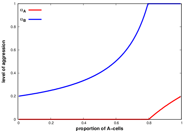If the proportion of $A$-cells is below a threshold ($x_{A}<\bar{x}_{A}$), in the ESS the larger $x_{A}$ is, the larger the expected payoff of the $A$-cells (see SI-Appendix A). Indeed, $A$-cells receive no aggression while $B$-cells receive more aggression as $x_{A}$ increases. In consequence, an $A$-cell more frequently obtains resource $v$, thus increasing its expected payoff. The expected payoff of an $A$-cell peaks when $x_{A}=\bar{x}_{A}$. Thereafter, the expected payoff of an $A$-cell starts decreasing. The explanation is that $A$-cells start fighting among themselves for resource $v$.

Tumors with high ITH. Consider a heterogeneous tumor formed by $A$-cells (in proportion $x_{A}$), $E$-cells (in proportion $x_{E}$) and $B$-cells (in proportion $x_{B}=1-x_{A}-x_{E}$). A 3-type population game is denoted by $\Gamma_{3}(v,c,x_{A},x_{E})$, as it can be defined by parameters $v$, $c$, and the proportions of $A$-cells and $E$-cells.

A strategy is denoted by ($\alpha_{A},\alpha_{B},\alpha_{E}$) where $\alpha_{I}$ is the probability of behaving aggressively when facing an $I$-cell ($I=A,B,E$). If an $I$-cell plays ($\alpha_{A},\alpha_{B},\alpha_{E}$) against an opponent playing ($\beta_{A},\beta_{B},\beta_{E}$) its expected payoff is the sum of the probability of meeting a cell of its own type, i.e., $(nx_{I}-1)/(n-1)$, multiplied by $u(\alpha_{I},\beta_{I})$, and the probability of meeting a cell of each other cell type, i.e., $(nx_{J})/(n-1)$, multiplied by $u(\alpha_{J},\beta_{I})$. Denoting the expected payoff of an $I$-cell by $U_{I}$, the following is obtained:

Observe that whenever cells choose the same strategy, which in equilibrium is always the case, the larger the payoff is the smaller the aggression that a cell type receives is. That is, $U_{I}>U_{J}$ is equivalent to $\alpha_{I}<\alpha_{J}$ (for $I,J\in\{{A,B,E\}}$).

Given that a cell does not know its own type, what can be maximized is the expected payoff of a generic cell, denoted by $U$, given by the sum of the probability of being $I$ multiplied by the expected payoff of an $I$-cell:

To be consistent with the hierarchy of cell types established above, we focus on the ESS where the three different types receive different expected payoffs such that $U_{A}>U_{B}>U_{E}$. The following proposition (See SI-Appendix B) indicates that the ESS depends on the proportions of the $A$-cells and $E$-cells.

Proposition 1: Let $\Gamma_{3}(v,c,x_{A},x_{E})$ be a 3-type population game. Thus, there exists an ESS with $U_{A}>U_{B}>U_{E}$ if and only if $x_{A}<\bar{x}_{A}$ and $x_{E}<\bar{x}_{E}$, where $\bar{x}_{E}=\frac{v}{c}\left(1-\frac{1}{n}\right)$. The ESS is given by:

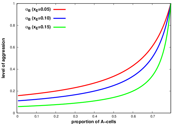
As expected, $A$-cells receive less aggression than $B$-cells, which in turn receive less aggression than $E$-cells ($\alpha_{A}<\alpha_{B}<\alpha_{E}$). The best-off cells do not receive any aggression, $B$-cells receive some aggression and $E$-cells receive full aggression. Figure 2 plots the aggression suffered by $B$-cells in the ESS for different proportions of $A$-cells and $E$-cells, showing that: (i) the larger $x_{A}$, the greater the aggression suffered by $B$-cells; and (ii) the larger $x_{E}$, the lesser the aggression suffered by $B$-cells (see SI-Appendix C).

Since only the expected payoff of the best-off $A$-cells is of interest in this context, we present the expected payoff in the ESS of those cells, denoted by $U_{A}^{\ast\ast\ast}(x_{A},x_{E})$. This is given by:

The larger $x_{A}$ is, the larger the expected payoff of each $A$-cell is (See SI-Appendix D). Indeed, the aggression towards $B$-cells increases while $A$-cells receive no aggression (and $E$-cells receive full aggression). As a result, an $A$-cell obtains resource $v$ more often and its expected payoff therefore increases. By contrast, the larger $x_{E}$ is, the smaller the expected payoff of each $A$-cell is. As $x_{E}$ increases two opposite effects are at play: On the one hand there are more $E$-cells, which receive full aggression, increasing overall aggression levels, which is beneficial for $A$-cells. On the other hand, as $x_{E}$ increases the aggression received by $B$-cells decreases, which reduces overall aggression, which is detrimental for $A$-cells. This negative effect turns out to outweigh the positive effect, so the expected payoff of each $A$-cell decreases with $x_{E}$.

An important point to highlight here is that there is no ESS with $U_{A}>U_{B}>U_{E}$ when the proportion of $A$-cells or $E$-cells exceed thresholds $\bar{x}_{A}$ or $\bar{x}_{E}$. Having $x_{A}>\bar{x}_{A}$ or $x_{E}>\bar{x}_{E}$ does not prevent the existence of ESS. In these cases two cell types receive an identical expected payoff: Either $U_{A}>U_{B}=U_{E}$ or $U_{A}=U_{B}>U_{E}$, thus reproducing a 2-type population game. This can be illustrated for the case $U_{A}>U_{B}=U_{E}$.

Proposition 2: Let $\Gamma_{3}(v,c,x_{A},x_{E})$ be a 3-type population game. There exists an ESS with $U_{A}>U_{B}=U_{E}$ for $x_{A}>\bar{x}_{A}$, given by

In this ESS, the $E$-cells are not distinguished from the $B$-cells ($\alpha_{B}=\alpha_{E}$). The level of aggression received and the expected payoffs are identical to those obtained in the ESS in the 2-type population game.

Comparison of heterogeneous tumors. The main question here concerns the comparison of the expected payoff of the best-off $A$-cells in the 2-type and 3-type population games. Clearly, the comparison is pertinent for equal proportions of $A$-cells in the two tumors under analysis. The following proposition (See SI-Appendix E) indicates when the expected payoff of an $A$-cell in ESS is strictly larger in the 2-type population game than in the 3-type population game.

Proposition 3: Let $y_{A}$ be a proportion of A-cells and let $\Gamma_{2}(v,c,y_{A})$ and $\Gamma_{3}(v,c,y_{A},x_{E})$ with $y_{a}<\bar{x}_{A}$ and $x_{E}<\bar{x}_{E}$. Then $U_{A}^{\ast\ast}(y_{A})>U_{A}^{\ast\ast\ast}(y_{A},x_{E})$.

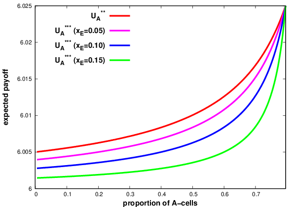
This result is illustrated in Figure 3. Recall that the ESS for $x_{A}<\bar{x}_{A}$ in $\Gamma_{2}(v,c,x_{A})$ is $\left(0,\tfrac{n-1}{n-nx_{A}-1}\tfrac{v}{c}\right)$ while the ESS in $\Gamma_{3}(v,c,x_{A},x_{E})$ is $\left(0,\frac{(n-1)v/c-nx_{E}}{n-nx_{A}-nx_{E}-1},1\right)$. In both games the best-off $A$-cells receive no aggression, while $E$-cells receive full aggression in the 3-type population game. $B$-cells receive some aggression in both games. The aggression received by $B$-cells in the 2-type population game is greater than that which they receive in the 3-type population game. This difference confers an advantage to $A$-cells in the former.

Translation in the oncology context. Proposition 1 indicates that an ESS in a 3-type population game only exists when the proportions of the best-off and worst-off cells do not exceed certain thresholds, $\bar{x}_{A}$ and $\bar{x}_{E}$. Therefore patients with tumors displaying a high ITH and a large proportion of the highest grade cells are not expected to be found. In other words, branching-type tumors should not display predominant proportions of the highest grade cells.

According to Proposition 2, beyond the thresholds for the best-off and worst-off cells, there is no ESS that distinguishes between the three types of cells in the 3-type population games since only two types can be distinguished. This means that once the proportion of the highest grade cells becomes large the ITH decreases. A branching-type tumor may thus become punctuated.

Proposition 3 shows that the best-off cell obtains a larger expected payoff in 2-type population games than in 3-type population games (for equal proportions of $A$-cells). This means that if two tumors with equal proportion of the highest grade are compared the one with the higher ITH should be less aggressive than the one with the lower ITH. In other words, for a given grade a branching-type tumor pursues a less aggressive course than a punctuated-type one.

The pathologists in the study retrospectively analyzed a series of 20 clear cell renal cell carcinomas (CCRCC) from archives of the Department of Anatomic Pathology at Cruces University Hospital (Barakaldo, Spain). Table 1 gives the main data of the series: Basic data on the patient (age and sex), number of regions analyzed, characteristics of the tumors (grade, heterogeneity), follow-up information, and the clinical situation of the patient.

The histological grade of a tumor is one of several measures that define its level of malignancy, i.e. biological aggressiveness. The ways in which pathologists assign a grade to a tumor under the microscope vary widely from one tumor entity to another. In general, the spectrum of grades in a tumor oscillates between grades 1 and 4, where the higher the grade is, the more aggressive the tumor is expected to be. The proportion of the highest nuclear grade detected appears in the table. In our modeling, this corresponds to the proportion of the best-off $A$-cells, $x_{A}$.

ITH measures the cellular variability detected in the tumor, a characteristic which is routinely assessed in modern pathology. Two levels are considered in the table: Low ITH is considered to exist when no more than two different grades are detected and high ITH when three or more different grades are seen.

Of the 12 patients with tumors showing low ITH, seven died of disease, four were alive with disease, and one was alive without the disease at last contact. All patients with tumors showing high ITH were alive without the disease at last contact. Comparative survival rates show that the difference between low and high ITH is statistically significant (log-rank $p<0.001$). Note that the comparison involves tumors with different grades and different proportions. A higher grade and a large proportion of the highest grade are generally associated with a worse clinical evolution of the patient. This may explain the prognoses of patients with grade 4 tumors and high proportions of the most malignant cells, all but two of whom (patients 3 and 19) died of the disease.

To check Proposition 3 we need to compare tumors of identical grades and similar (if not identical) proportions of the highest grade. Five out of the six grade 3 tumors have similar proportions of the highest grade ($x_{A}$ between $5\%$ and $20\%$). It can be observed that the three patients with tumors that show high ITH (patients 15, 17, and 20) are alive without the disease while the two with low ITH tumors are alive with the disease (1, and 16). This finding is consistent with Proposition 3, assuming that $\bar{x}_{A}>20\%$. Note that patient 20, with a highly heterogeneous tumor of proportion $x_{A}=20\%$, is alive without the disease, while patients 1 and 16 with low heterogeneous tumors of proportion $x_{A}=10\%$, are alive with the disease.

According to Proposition 1 patients with tumors displaying a high ITH and a large proportion of the highest grade cells are not expected to be found. We indeed observe that the six tumors with high ITH have small proportions of the highest grade cells ($x_{A}<20\%$).

This paper looks at the hawk-dove game in heterogeneous populations. The main assumption in this context is that cells are programmed to adopt a specific behavior according to the behavior of cells with which they interact. As a result, different cells are treated differently and obtain different fitness levels. The difference in terms of fitness in a cell depends only on the different behaviors adopted by the remaining cells, and not on its own behavior.

The spectrum of cell variability in a tumor is an important characteristic routinely assessed in modern pathology. Our study suggests that this characteristic may be correlated with tumor aggressiveness. Here, mathematical findings are supported by histological and genomic data. For example, a basic histological study of 20 CCRCC exhaustively sampled and followed clinically for at least 5 years confirms that aggressive forms of CCRCC show low levels of ITH. Moreover, a genomic study of a series of 101 CCRCC has shown that tumors with low ITH and a punctuated-type evolutionary pattern pursue an aggressive clinical course, with early and multiple metastases, whereas tumors with high ITH and branching-type evolution show a more attenuated clinical course, with late, solitary metastases [4]. Our study suggests also that branching-type tumors may, under specific conditions, evolve into punctuated-type tumors. This evolution has been detected in several types of malignant tumors [19].

At a practical level, our results support the idea that it is appropriate to preserve high ITH in tumors as a promising therapeutic strategy. Thus, a therapy aimed at tumor containment should be more effective than administrating the conventional maximum tolerable dose because the latter strategy would force tumor cells to develop different clones able to survive as soon as possible [20]. As a result, a resistant-to-therapy neoplasm develops. Even if the tumor presents a high ITH before therapy, recurrence will result in a low ITH neoplasm. The maximum tolerable dose has already been questioned using a game theory approach [12].

The strategy of tumor containment seeks to diversify the energy expenditure of the cell by administrating drugs below the maximum tolerable dose [20]. Tumor cells will thus distribute their energy across different tasks, causing them to lose efficiency in all of them. The total amount of energy in the cell is limited, so all tumor cell functions will necessarily slow down. This will lead to retarded growth in tumors, the persistence of high ITH, and longer survival periods for patients.

In the 2-type population game the expected payoff of $A$-cells at the ESS increases with $x_{A}$ for $x_{A}<\bar{x}_{A}$ and decreases for $x_{A}>\bar{x}_{A}$.

In a 3-type population game strategy $\left(0,\frac{(n-1)v/c-nx_{E}}{n-nx_{A}-nx_{E}-1},1\right)$ is an ESS if $x_{E}<\bar{x}_{E}$ and $x_{A}<\bar{x}_{A}$.

The optimal choice of a cell given that its opponent plays $(\beta_{A},\beta_{B},\beta_{E})$ is to play $\alpha_{I}=1$ whenever $f_{I}(\beta_{A},\beta_{B},\beta_{E})>0$, $\alpha_{I}=0$ whenever $f_{I}(\beta_{A},\beta_{B},\beta_{E})<0$ and $\alpha_{I}\in[0,1]$ whenever $f_{I}(\beta_{A},\beta_{B},\beta_{E})=0$ where $I=A,B,E$. If its opponent plays $\left(0,\beta_{B},1\right)$ the optimal choice of a cell is $\alpha_{A}=0$, $\alpha_{B}=\beta_{B}$ (with $0\leq\alpha_{B}\leq 1$) and $\alpha_{E}=1$ as long as $f_{A}\left(0,\beta_{B},1\right)<0$, $f_{B}\left(0,\beta_{B},1\right)=0$ and $f_{E}\left(0,\beta_{B},1\right)>0$.

Equality $f_{B}\left(0,\beta_{B},1\right)=0$ is satisfied if $\frac{v}{c}\left(1-\frac{1}{n}\right)-(1-x_{A}-x_{E})\beta_{B}-x_{E}+\frac{\beta_{B}}{n}=0$ or equivalently $\frac{v}{c}\left(n-1\right)-(n-nx_{A}-nx_{E})\beta_{B}-nx_{E}+\beta_{B}=0$, leading to $\beta_{B}=\frac{(n-1)v/c-nx_{E}}{n-nx_{A}-nx_{E}-1}$.

Condition $\beta_{B}>0$ gives $(n-1)v/c-nx_{E}$ $>0$ or equivalently $x_{E}<\bar{x}_{E}$ (assuming there is strictly more than one cell of each type, i.e., $nx_{B}=n-nx_{A}-nx_{E}>1$).

Condition $\beta_{B}<1$ gives $(n-1)v/c-nx_{E}<n-nx_{A}-nx_{E}-1$, or $x_{A}<\bar{x}_{A}$. It remains to verify that $f_{A}\left(0,\frac{(n-1)v/c-nx_{E}}{n-nx_{A}-nx_{E}-1},1\right)<0$ and $f_{E}\left(0,\frac{(n-1)v/c-nx_{E}}{n-nx_{A}-nx_{E}-1},1\right)>0$ hold at $\left(0,\frac{(n-1)v/c-nx_{E}}{n-nx_{A}-nx_{E}-1},1\right)$, which with simple algebraic manipulations can be proved that is true.

Second, it remains to verify that strategy $\left(0,\frac{(n-1)v/c-nx_{E}}{n-nx_{A}-nx_{E}-1},1\right)$ which is a best response to $\left(0,\frac{(n-1)v/c-nx_{E}}{n-nx_{A}-nx_{E}-1},1\right)$ cannot be invaded by a mutant strategy.

Let the opponent play $(\gamma_{A},\gamma_{B},\gamma_{E})$, as a best response to $\left(0,\frac{(n-1)v/c-nx_{E}}{n-nx_{A}-nx_{E}-1},1\right)$. We have to check that the expected payoff obtained when playing $\left(0,\frac{(n-1)v/c-nx_{E}}{n-nx_{A}-nx_{E}-1},1\right)$ is larger than when it is playing $(\gamma_{A},\gamma_{B},\gamma_{E})$. As checked above $f_{A}\left(0,\frac{(n-1)v/c-nx_{E}}{n-nx_{A}-nx_{E}-1},1\right)<0$, $f_{B}\left(0,\frac{(n-1)v/c-nx_{E}}{n-nx_{A}-nx_{E}-1},1\right)=0$ and $f_{E}\left(0,\frac{(n-1)v/c-nx_{E}}{n-nx_{A}-nx_{E}-1},1\right)>0$. Thus, we have $\gamma_{A}=0$, $0<\gamma_{B}<1$, and $\gamma_{E}=1$. Then, from (B.1) we write the difference of expected payoffs when playing $\left(0,\frac{(n-1)v/c-nx_{E}}{n-nx_{A}-nx_{E}-1},1\right)$ and $\left(0,\gamma_{B},1\right)$ whenever the opponent plays $\left(0,\gamma_{B},1\right)$:

Thus, the expected payoff is strictly larger playing $\left(0,\frac{(n-1)v/c-nx_{E}}{n-nx_{A}-nx_{E}-1},1\right)$ than $\left(0,\gamma_{B},1\right)$ and strategy $\left(0,\frac{(n-1)v/c-nx_{E}}{n-nx_{A}-nx_{E}-1},1\right)$ is an ESS.  

In a 3-type population game, the aggression suffered by $B$-cells at the ESS increases with the proportion of $A$-cells, $x_{A}$; while it decreases with the proportion of $E$-cells, $x_{E}$.

Therefore, for $x_{A}<\bar{x}_{A}$ and $x_{E}<\bar{x}_{E}$ at the ESS, we have $\frac{\partial\alpha_{B}^{*}}{\partial x_{A}}>0$ and $\frac{\partial\alpha_{B}^{*}}{\partial x_{E}}<0$.  

In the 3-type population game the expected payoff of each $A$-cell at the ESS increases with $x_{A}$ and decreases with $x_{E}$.

Therefore, we have $\frac{\partial}{\partial x_{A}}\left[U_{A}^{\ast\ast\ast}(x_{A},x_{E})\right]>0$ and $\frac{\partial}{\partial x_{E}}\left[U_{A}^{\ast\ast\ast}(x_{A},x_{E})\right]<0$.  

For $x_{A}<\bar{x}_{A}$ and $x_{E}<\bar{x}_{E}$ we have $U_{A}^{**}(x_{A})>U_{A}^{***}(x_{A},x_{E})$.

References

- [1] Dentro, S. C., Leshchiner, I., Haase, K., Tarabichi, M., Wintersinger, J., Deshwar, A. G. et al. (2021) Characterizing genetic intra-tumor heterogeneity across 2,658 human cancer genomes. Cell 184: 2239-2254.
- [2] Tong, M., Deng, Z., Zhang, X. et al. (2018) New insights from the widening homogeneity perspective to target intratumor heterogeneity. Cancer Commun 38, 17.
- [3] Thomas, F., Roche, B., Giraudeau, M., Hamede, R., Ujvari, B. (2020) The interface between ecology, evolution, and cancer: More than ever a relevant research direction for both oncologists and ecologists. Evol Appl 13: 1545-1549.
- [4] Turajlic, S., Xu, H., Litchfield, K. et al. (2018) Deterministic evolutionary trajectories influence primary tumor growth: TRACERx Renal. Cell 173: 595-610.
- [5] Davis, A., Gao, R., Navin, N. (2017) Tumor evolution: Linear, branching, neutral or punctuated? Biochem Biophys Acta 1867: 151-161.
- [6] Axelrod, R., Pienta, K. L. (2018) Cancer as a social dysfunction. Why cancer research needs new thinking. Mol Cancer Res 16: 1346-1347.
- [7] Dingli, D., Chalub, F. A., Santos, F. C., Pacheco, J. (2009) Cancer phenotype as the outcome of an evolutionary game between normal and malignant cells. Br. J. Cancer 101, 1130-1136.
- [8] Archetti M., Pienta K. J. (2019) Cooperation among cancer cells: applying game theory to cancer. Nat Rev Cancer 19: 110-117.
- [9] Wölfl, B., te Rietmole, H., Salvioli, M., Kaznatcheev, A., Thuijsman, F., Brown, J. S., Burgering, B., Stankova, K. (2021) The Contribution of Evolutionary Game Theory to Understanding and Treating Cancer, Dyn Games Appl, doi: 10.1007/s13235-021-00397-w.
- [10] McEvoy J. W. (2009) Evolutionary game theory: lessons and limitations, a cancer perspective. Br J Cancer 101: 2060-2061.
- [11] Errarte P., Larrinaga G., López J. I. (2020) The role of cancer-associated fibroblasts in renal cell carcinoma. An example of tumor modulation through tumor/non-tumor cell interactions. J Adv Res 21: 103-108.
- [12] Archetti M. (2021) Collapse of Intra-Tumor Cooperation Induced by Engineered Defector. Cells Cancer 13, 3674.
- [13] De la Fuente I. M., Cortés J. M., Valero E., Desroches M., Rodrigues S., Malaina I., Martínez L. (2014) On the dynamics of the adenylate energy system: homeorhesis vs homeostasis. PLoS One 9: e108676.
- [14] Inarra, E., Laruelle, A. (2012) Artificial Distinction and Real Discrimination, Journal of Theoretical Biology 305, 110-117.
- [15] Maruyama T., Fujita Y. (2017) Cell competition in mammals. Novel homeostatic machinery for embryonic development and cancer prevention. Curr Opin Cell Biol 48: 106-112.
- [16] Maynard Smith, J. (1982) Evolution and the theory of games, Cambridge University Press; Cambridge, UK.
- [17] Maynard Smith, J., Price, G. R. (1973) The Logic of Animal Conflict, Nature 246, 15-18.
- [18] Maynard Smith, J., Parker, G. A. (1976) The Logic of Asymmetric Contests, Animal Behaviour 24, 159-175.
- [19] Bao Z., Wang Y., Wang Q., Fang S., Shan X., Wang J., Jiang T. (2021) Intratumor heterogeneity, microenvironment, and mechanisms of drug resistance in glioma recurrence and evolution. Front Med. 15: 551-561.
- [20] Gundem, G.; Van Loo, P.; Kremeyer, B.; Alexandrov, L.B.; Tubio, J.M.C.; Papaemmanull, E.; et al. (2015) The evolutionary history of lethal metastatic prostate cancer. Nature 520, 353-357, doi: 10.1038/nature14347.
Supporting Information - Appendix A