跳到论文正文
W Papers独立论文阅读器 arXiv:2202.02184 论文正文 计算阅读时间 · 0%
引用这篇论文根据当前论文元数据生成,正式投稿前建议核对。


License: CC BY 4.0
arXiv:2202.02184v4 [quant-ph] 19 Mar 2023

Singleton Bounds for Entanglement-Assisted
Classical and Quantum Error Correcting CodesA short version of this work has been presented at ISIT 2022 and is included in its proceedings EACQ-Singleton-ISIT.

Manideep Mamindlapally  Email: manideepyx@iitkgp.ac.in Affiliation: IIT Kharagpur, Kharagpur, India - 721302    Andreas Winter  Email: andreas.winter@uab.cat Affiliation: ICREA & Grup d’Informació Quàntica, Departament de Física, Universitat Autònoma de Barcelona, 08193 Bellaterra (BCN), Spain Affiliation: Institute for Advanced Study, Technische Universität München, Lichtenbergstraße 2a, D-85748 Garching, Germany
17 March 2023
Abstract

We show that entirely quantum Shannon theoretic methods, based on von Neumann entropies and their properties, can be used to derive Singleton bounds on the performance of entanglement-assisted hybrid classical-quantum (EACQ) error correcting codes. Concretely, we show that the triple-rate region of qubits, cbits and ebits of possible EACQ codes over arbitrary alphabet sizes is contained in the quantum Shannon theoretic rate region of an associated memoryless erasure channel, which turns out to be a polytope. We show that a large part of this region is attainable by certain EACQ codes, whenever the local alphabet size (i.e. Hilbert space dimension) is large enough, in keeping with known facts about classical and quantum maximum distance separable (MDS) codes: in particular, all of its extreme points and all but one of its extremal lines. The attainability of the remaining one extremal line segment is left as an open question.

I Introduction

Quantum error correcting codes (QECC) are subject to various universal constraints relating block length, alphabet size, minimum distance and code rate, very much like classical error correcting codes. In particular, the classical Singleton bound Singleton has a satisfying quantum version for QECC q-Singleton; q-Singleton-Rains; KlappeneckerSarvepalli:subsystem-Singleton, which has been extended to entanglement-assisted and catalytic QECC (EAQECC and CQECC) ea-q-Singleton; catalytic-q-Singleton. Indeed, since their proposal, EAQECC have enjoyed considerable attention from coding theorists, both in the block coding and the convolutional coding setting Galindo-et-al; LaiBrun:imperfect; Nadkarni; Allahmadi-et-al; Chen:ea; LaiAshikhmin; WildeBrunBabar:EA-turbo. Note that the original EAQECC Singleton bound was found to be erroneous in general Grassl-counterex, which was put right in the recent paper EAQECC-Singleton. Although these bounds all have different forms, they are united in that they express the ability of the code to correct erasure errors. Classically, the Singleton bound is attained for MDS codes, which exist for sufficiently large alphabet size. Similarly, attaining these quantum Singleton bounds defines suitable quantum MDS (QMDS) codes and their entanglement-assisted generalisations.

The present paper grew out of an attempt to understand better the results of EAQECC-Singleton, where the most complete quantum Singleton bound so far was derived for EAQECC, in the form of a two-dimensional convex region in the ebit-qubit plane, into which all possible codes necessarily fall (as a function of block length and minimum distance). Investigating the tightness of the bound exhibited two types of codes attaining the boundary of the allowed region, one a genuinely entanglement-assisted quantum code dubbed EAQ, the other a classical MDS code piggy-backed onto a simple teleportation protocol. This suggested that, to obtain a full understanding of the codes involved, one should extend the investigation to hybrid classical and quantum codes, assisted by entanglement (EACQ codes), which we provide here. As our main result, we prove Singleton bounds for such EACQ codes, in the form of a convex triple-tradeoff region in the ebit-cbit-qubit space (as a function of block length and minimum distance).

Hybrid classical and quantum error correcting codes have been considered in several papers before, mostly without entanglement-assistance GrasslLuZeng:hybrid; NemecKlappi:hybrid; NemecKlappi:hybrid-paper; Cao-et-al:hybrid; NemecKlappi:hybrid-detecting; the EACQ codes as considered by us have been introduced in KremskyHsiehBrun, although we allow additionally catalysis (recycling) of the three basic resources, making our bounds more general. Classical and quantum hybrid error correcting codes have been generalised in beny2007generalization; beny2007PRA; Majidy:hybrid; NemecKlappi:subsystem-hybrid to classical and quantum hybrid subsystem codes in an operator algebraic setting. We stress that our bounds apply to either kind of code. Importantly for our approach, the triple tradeoff between ebits, cbits and qubits has been treated repeatedly in the Shannon-theoretic setting of a given channel (often i.i.d. on the block of nn physical systems) and small errors. A precursor was the breakthrough paper by Devetak and Shor devetak2005capacity, which showed how to analyse the capacity region of joint classical and quantum information transmission over a given noisy channel. For us, the paper by Hsieh and Wilde HsiehWilde is fundamental, which derives a multi-letter capacity formula for the triple tradeoff, of which we take the converse proof and develop it in several directions. We follow essentially the very developed, rigorous exposition of Wilde (wildebeast, Ch. 25).

Results. We give here an overview of our main results, which also serves as a guide to the paper. In Section II we review the definition of EACQ codes and pose the problem of characterising all triples of catalytic rates attainable for given block length and minimum distance, and then discuss preliminaries in Section III. After that:

  • •

    We state Hsieh-Wilde’s converse theorem ((HsiehWilde, Thm. 1)) in Section IV and give a complete proof from first principles, and generalised both to arbitrary (one-shot) channels and the catalytic setting, in the Appendix A, the latter having previously been accomplished in (wildebeast, Ch. 25).

  • •

    We use this general converse to derive the triple-tradeoff rate region for the i.i.d. erasure channel, correcting a gap in HsiehWilde, where the erasure probability δ\delta was assumed to be less than 12\frac{1}{2}, in Section V. (Wilde (wildebeast, Ch. 25.5.3) is much more complete, but proves additivity only for δ≤12\delta\leq\frac{1}{2}.)

  • •

    We then use the general one-shot converse for a channel that randomly erases d−1d-1 of the nn physical systems and with error probability set to 00, to derive the Singleton bound for EACQ codes, subsuming both classical Singleton bounds and all previously known quantum Singleton bounds; the obtained region is the same as for an i.i.d. erasure channel with erasure probability δ=d−1n\delta=\frac{d-1}{n}, in Section VI.

  • •

    We analyse the geometric shape of the EACQ Singleton region, determining its extreme points and extremal lines; we can then show that large parts of the boundary are indeed attained, whenever the alphabet size is large enough, in Section VII. One line segment remains to be shown to be attainable, to prove our entire region to be optimal, which we leave as an open question, and which we discuss among other things in the concluding Section VIII.

II Problem Setting

Following (wildebeast, Ch. 25), we begin by defining the task of hybrid classical and quantum communication via a noisy channel, i.e. a linear completely positive and trace preserving (cptp) map 𝒩:ℒ⁡(A)→ℒ⁡(B){\cal N}\mathrel{\mathop{\mathchar 58\relax}}{\cal L}(A)\rightarrow{\cal L}(B), assisted by entanglement, in the one-shot setting and allowing for a certain (small) decoding error. Here, AA and BB are complex Hilbert spaces associated to the quantum systems of sender and receiver, which for convenience we will throughout assume to be of finite dimension; ℒ⁡(A){\cal L}(A) is the space of all linear operators (matrices) on AA, and likewise for BB.

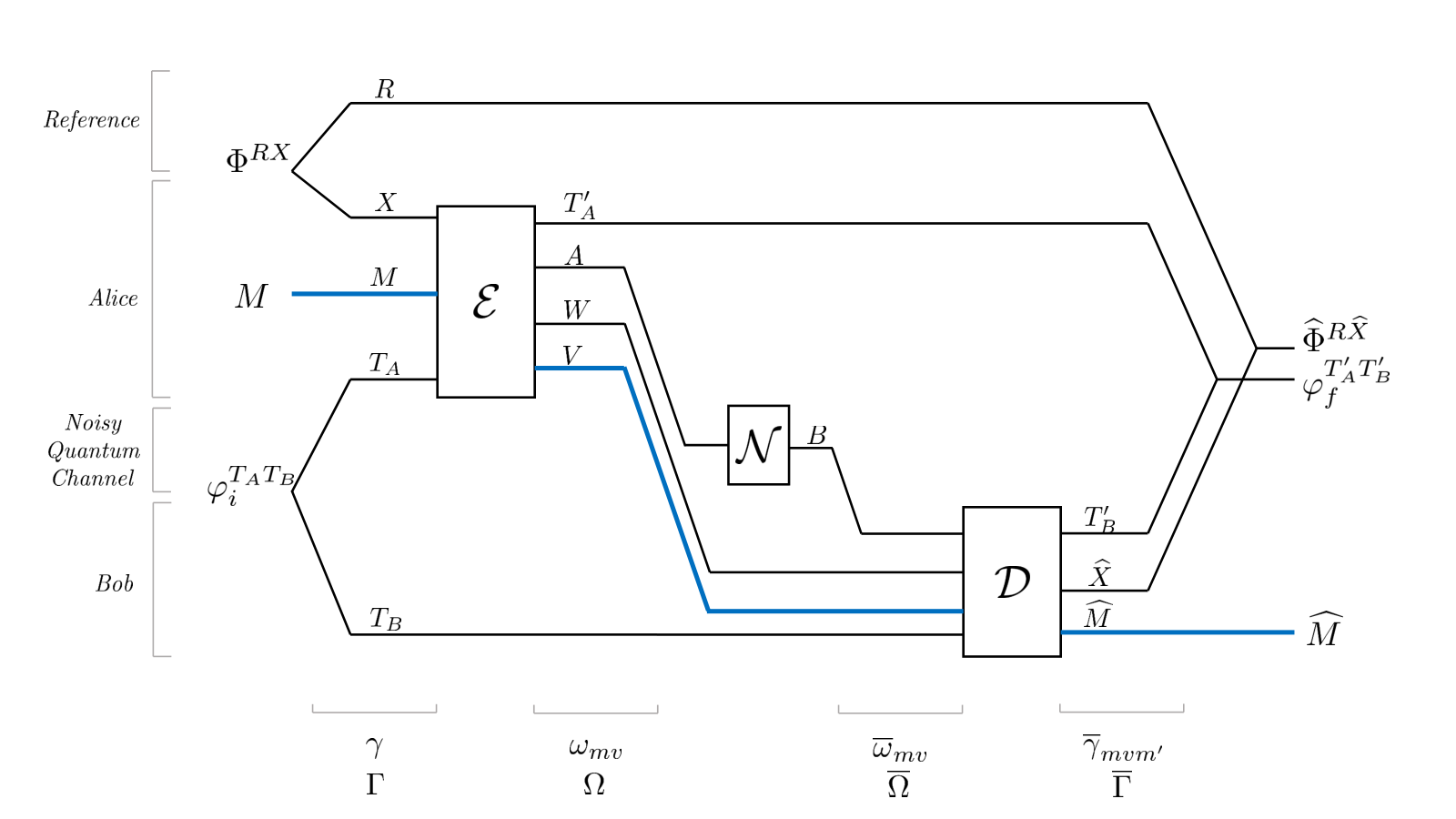
Refer to caption
Figure 1: Communication diagramme of the most general catalytic entanglement-assisted classical and quantum code. We discuss four snapshots of the involved systems at different times, at which we wish to analyse their joint state: at starting time (initial state Γ\Gamma), after the encoding (Ω\Omega), after the action of the noisy channel (Ω¯\overline{\Omega}), and after the decoding (Γ¯\overline{\Gamma}). The starting quantum systems XX and RR constitute Q2Q_{2} qubits each, the message MM has C2C_{2} cbits, and the entangled systems TAT_{A} and TBT_{B} carry an equivalent of E1E_{1} pure entangled ebits. The intermediate system WW carries Q1Q_{1} qubits and VV carries C1C_{1} cbits. The input system AA is passed through a noisy channel 𝒩{\cal N} to produce output system BB. On decoding, the output quantum system X^\hat{X} contains Q2Q_{2} qubits, the output classical message M^\hat{M} has C2C_{2} cbits. Additionally, a system TB′T_{B}^{\prime} is generated that has E2E_{2} ebits of entanglement with Alice’s system TA′T_{A}^{\prime}.

We consider a general entanglement-assisted classical and quantum communication setup as in Fig. 1. We have communicating agents, a sender Alice and a receiver Bob. Apart from the channel 𝒩{\cal N}, they start with (a) a shared entangled quantum state φiTA​TB\varphi_{i}^{T_{A}T_{B}} of E1=S⁡(φiTA)E_{1}=S(\varphi_{i}^{T_{A}}) ebits, (b) a quantum channel capable of transmitting Q1Q_{1} qubits, (c) a classical channel capable of transmitting C1C_{1} cbits. Using encoding and decoding operations, they wish to achieve (a) transfer of Q2Q_{2} qubits of quantum information, (b) transfer of C2C_{2} cbits of classical information, and (c) regeneration of E2=S⁡(φfTA′)E_{2}=S(\varphi_{f}^{T_{A}^{\prime}}) ebits of shared entanglement in the form of a shared state φfTA′​TB′\varphi_{f}^{T_{A}^{\prime}T_{B}^{\prime}}. This results in a net transfer of Q=Q2−Q1Q=Q_{2}-Q_{1} qubits, C=C2−C1C=C_{2}-C_{1} cbits on using up of E=E1−E2E=E_{1}-E_{2} ebits. The entire diagram, defined by the maps 𝒟{\cal D} and ℰ{\cal E} is called an entanglement-assisted classical and quantum error correcting code (EACQ code) of error ϵ\epsilon for the channel 𝒩{\cal N}. We speak simply of an EACQ code if the error is implied to be ϵ=0\epsilon=0. Furthermore, for an nn-partite input system An=A1​…​AnA^{n}=A_{1}\ldots A_{n} composed of AjA_{j} that are all qq-dimensional Hilbert spaces, we say that an EACQ code has minimum distance dd if it has error ϵ=0\epsilon=0 for the following block erasure channel, which uniformly randomly erases d−1d-1 out of nn of the system AiA_{i}:

ℰq,d−1,n(ρ)=1(nd−1)∑J⊂[n],|J|=d−1(TrAJρ)B[n]∖J⊗|⟂⟩⟨⟂|BJ,{\cal E}_{q,d-1,n}(\rho)=\frac{1}{{n\choose d-1}}\sum_{J\subset[n],\atop|J|=d-1}\left(\operatorname{Tr}_{A_{J}}\rho\right)^{B_{[n]\setminus J}}\otimes|\perp\rangle\!\langle\perp|^{B_{J}}, (1)

where Bj=Aj⊕C⁡|⟂⟩B_{j}=A_{j}\oplus{{\mathbb C}}|\perp\rangle and |⟂⟩BJ=⨂j∈J|⟂⟩Bj|\perp\rangle^{B_{J}}=\bigotimes_{j\in J}|\perp\rangle^{B_{j}}. We adopt the taxonomy of KremskyHsiehBrun for an EACQ code of block length nn and minimum distance dd: it is denoted [[n,k:c,d;e]]q[\![n,k\mathrel{\mathop{\mathchar 58\relax}}c,d;e]\!]_{q}, where k=Qlog⁡qk=\frac{Q}{\log q}, c=Clog⁡qc=\frac{C}{\log q} and e=Elog⁡qe=\frac{E}{\log q}.

The objective now is to chararacterise the permissible values of CC, QQ and EE for a given block length nn such that a code with small or vanishing error exists. To formalize this, we analyse the states describing all involved systems at four different times and then define an associated error term. In the beginning, the initial states are prepared:

γR​X​TA​TB\displaystyle\gamma^{RXT_{A}T_{B}} =ΦR​X⊗φiTA​TB,\displaystyle=\Phi^{RX}\otimes\varphi_{i}^{T_{A}T_{B}},
ΓM​R​X​TA​TB\displaystyle\Gamma^{MRXT_{A}T_{B}} =∑m∈ℳ1|ℳ|​|m⟩​⟨m|M⊗γR​X​TA​TB.\displaystyle=\sum_{m\in{\cal M}}\frac{1}{|{\cal M}|}|m\rangle\langle m|^{M}\otimes\gamma^{RXT_{A}T_{B}}. (2)
On encoding using a collection of CPTP maps (ℰv|mX​TA→TA′​A​W)v∈𝒱\left({\cal E}_{v|m}^{XT_{A}\rightarrow T_{A}^{\prime}AW}\right)_{v\in{\cal V}} on classical input m∈ℳm\in{\cal M}, we have:
pV|M​(v|m)\displaystyle p_{V|M}(v|m) =Tr⁡ℰv|mX​TA→TA′​A​W​(γR​X​TA​TB),\displaystyle=\operatorname{Tr}{\cal E}_{v|m}^{XT_{A}\rightarrow T_{A}^{\prime}AW}\left(\gamma^{RXT_{A}T_{B}}\right),
ωm​vR​TA′​A​W​TB\displaystyle\omega_{mv}^{RT_{A}^{\prime}AWT_{B}} =1pV|M​(v|m)​ℰv|mX​TA→TA′​A​W​(γR​X​TA​TB),\displaystyle=\frac{1}{p_{V|M}(v|m)}{\cal E}_{v|m}^{XT_{A}\rightarrow T_{A}^{\prime}AW}\left(\gamma^{RXT_{A}T_{B}}\right),
ΩM​V​R​TA′​A​W​TB\displaystyle\Omega^{MVRT_{A}^{\prime}AWT_{B}} =∑m∈ℳv∈𝒱1|ℳ|​pV|M​(v|m)​|m​v⟩​⟨m​v|M​V⊗ωm​vR​TA′​A​W​TB.\displaystyle=\sum_{\begin{subarray}{c}m\in{\cal M}\\ v\in{\cal V}\end{subarray}}\frac{1}{|{\cal M}|}p_{V|M}(v|m)|mv\rangle\langle mv|^{MV}\otimes\omega_{mv}^{RT_{A}^{\prime}AWT_{B}}. (3)
After the action of the channel:
ω¯m​vR​TA′​B​W​TB\displaystyle\overline{\omega}_{mv}^{RT_{A}^{\prime}BWT_{B}} =𝒩A→B​(ωm​vR​TA′​A​W​TB),\displaystyle={\cal N}^{A\rightarrow B}\left(\omega_{mv}^{RT_{A}^{\prime}AWT_{B}}\right),
Ω¯M​V​R​TA′​B​W​TB\displaystyle\overline{\Omega}^{MVRT_{A}^{\prime}BWT_{B}} =∑m∈ℳv∈𝒱1|ℳ|​pV|M​(v|m)​|m​v⟩​⟨m​v|M​V⊗ω¯m​vR​TA′​B​W​TB.\displaystyle=\sum_{\begin{subarray}{c}m\in{\cal M}\\ v\in{\cal V}\end{subarray}}\frac{1}{|{\cal M}|}p_{V|M}(v|m)|mv\rangle\langle mv|^{MV}\otimes\overline{\omega}_{mv}^{RT_{A}^{\prime}BWT_{B}}. (4)
And finally, after decoding using a collection of CPTP maps (𝒟m′|vB​W​TB→X^​TB′)m′∈ℳ\left({\cal D}_{m^{\prime}|v}^{BWT_{B}\rightarrow\widehat{X}T_{B}^{\prime}}\right)_{m^{\prime}\in{\cal M}} on classical input v∈𝒱v\in{\cal V} to the decoder:
pM^|M​V​(m′|m​v)\displaystyle p_{\widehat{M}|MV}(m^{\prime}|mv) =Tr⁡𝒟m′|vB​W​TB→X^​TB′​(ω¯m​vR​TA′​B​W​TB),\displaystyle=\operatorname{Tr}{\cal D}_{m^{\prime}|v}^{BWT_{B}\rightarrow\widehat{X}T_{B}^{\prime}}\left(\overline{\omega}_{mv}^{RT_{A}^{\prime}BWT_{B}}\right),
γ¯m​v​m′R​X^​TA′​TB′\displaystyle\overline{\gamma}_{mvm^{\prime}}^{R\widehat{X}T_{A}^{\prime}T_{B}^{\prime}} =1pM^|M​V​(m′|m​v)​𝒟m′|vB​W​TB→X^​TB′​(ω¯m​vR​TA′​B​W​TB),\displaystyle=\frac{1}{p_{\widehat{M}|MV}(m^{\prime}|mv)}{\cal D}_{m^{\prime}|v}^{BWT_{B}\rightarrow\widehat{X}T_{B}^{\prime}}\left(\overline{\omega}_{mv}^{RT_{A}^{\prime}BWT_{B}}\right),
Γ¯M​V​M^​R​X^​TA′​TB′\displaystyle\overline{\Gamma}^{MV\widehat{M}R\widehat{X}T_{A}^{\prime}T_{B}^{\prime}} =∑m∈ℳv∈𝒱m′∈ℳ1|ℳ|​pV|M​(v|m)​pM^|M​V​(m′|m​v)​|m​v​m′⟩​⟨m​v​m′|M​V​M^⊗γ¯m​v​m′R​X^​TA′​TB′.\displaystyle=\sum_{\begin{subarray}{c}m\in{\cal M}\\ v\in{\cal V}\\ m^{\prime}\in{\cal M}\end{subarray}}\frac{1}{|{\cal M}|}p_{V|M}(v|m)p_{\widehat{M}|MV}(m^{\prime}|mv)|mvm^{\prime}\rangle\langle mvm^{\prime}|^{MV\widehat{M}}\otimes\overline{\gamma}_{mvm^{\prime}}^{R\widehat{X}T_{A}^{\prime}T_{B}^{\prime}}. (5)

The ideal output state pertaining to the quantum information is the maximally entangled state ΦR​X^=idX→X^⁡(ΦR​X)\Phi^{R\widehat{X}}={\operatorname{id}}^{X\rightarrow\widehat{X}}\left(\Phi^{RX}\right), the ideal final entanglement state is arbitrary, but has to be a pure state φfTA′​TB′\varphi_{f}^{T_{A}^{\prime}T_{B}^{\prime}}, and the ideal state pertaining to the classical information is the perfectly correlated classical state Φ¯M​M^=1|ℳ|​∑m|m⟩​⟨m|M⊗|m⟩​⟨m|M^\overline{\Phi}^{M\widehat{M}}=\frac{1}{|{\cal M}|}\sum_{m}|m\rangle\!\langle m|^{M}\otimes|m\rangle\!\langle m|^{\widehat{M}}. The ideal output is the product state

Γ¯idealM​M^​R​X^​TA′​TB′\displaystyle\overline{\Gamma}_{\text{ideal}}^{M\widehat{M}R\widehat{X}T_{A}^{\prime}T_{B}^{\prime}} =Φ¯M​M^⊗ΦR​X^⊗φfTA′​TB′.\displaystyle=\overline{\Phi}^{M\widehat{M}}\otimes\Phi^{R\widehat{X}}\otimes\varphi_{f}^{T_{A}^{\prime}T_{B}^{\prime}}. (6)

We say that the protocol (the code) has error ϵ\epsilon, if

12​‖Γ¯M​M^​R​X^​TA′​TB′−Γ¯idealM​M^​R​X^​TA′​TB′‖1≤ϵ,\frac{1}{2}\left\|\overline{\Gamma}^{M\widehat{M}R\widehat{X}T_{A}^{\prime}T_{B}^{\prime}}-\overline{\Gamma}_{\text{ideal}}^{M\widehat{M}R\widehat{X}T_{A}^{\prime}T_{B}^{\prime}}\right\|_{1}\leq\epsilon, (7)

where ‖X‖1=Tr⁡|X|=Tr⁡X†​X\|X\|_{1}=\operatorname{Tr}|X|=\operatorname{Tr}\sqrt{X^{\dagger}X} denotes the trace norm (aka Schatten-11-norm). Note that this implies, by the contractivity of the trace norm under partial trace and more generally cptp maps, that

Pr{M≠M^}=12‖Γ¯M​M^−Φ¯M​M^‖1\displaystyle\Pr\left\{M\neq\widehat{M}\right\}=\frac{1}{2}\left\|\overline{\Gamma}^{M\widehat{M}}-\overline{\Phi}^{M\widehat{M}}\right\|_{1} ≤ϵ,\displaystyle\leq\epsilon,
12​‖Γ¯R​X^−ΦR​X^‖1\displaystyle\frac{1}{2}\left\|\overline{\Gamma}^{R\widehat{X}}-\Phi^{R\widehat{X}}\right\|_{1} ≤ϵ,\displaystyle\leq\epsilon,
12​‖Γ¯TA′​TB′−φfTA′​TB′‖1\displaystyle\frac{1}{2}\left\|\overline{\Gamma}^{T_{A}^{\prime}T_{B}^{\prime}}-\varphi_{f}^{T_{A}^{\prime}T_{B}^{\prime}}\right\|_{1} ≤ϵ.\displaystyle\leq\epsilon.

As discussed at the start of this section, the other important parameters of the code are the initial entanglement E1=S⁡(φiTA)E_{1}=S\left(\varphi_{i}^{T_{A}}\right) (where SS denotes the von Neumann entropy), the invested qubit transmission Q1=log⁡|W|Q_{1}=\log|W| (with |W||W| denoting the dimension of the Hilbert space WW, for both see the next section), and the invested cbit transmission C1=log⁡|V|C_{1}=\log|V|; furthermore the final generated entanglement E2=S⁡(φfTA′)E_{2}=S\left(\varphi_{f}^{T_{A}^{\prime}}\right), the effected qubit transmission Q2=log⁡|X|Q_{2}=\log|X|, and the effected cbit transmission C2=log⁡|M|C_{2}=\log|M|. In the sequel we will derive bounds on the net (also called amortized) rates E=E1−E2E=E_{1}-E_{2}, Q=Q2−Q1Q=Q_{2}-Q_{1} and C=C2−C1C=C_{2}-C_{1}. Note the different treatment of the net entanglement rate, in two ways: first, it is defined in terms of entropies rather than a logarithmic dimension, so as not to restrict to maximal entanglement as initial or final state (but if φi\varphi_{i} or φf\varphi_{f} is maximally entangled, then E1=log⁡|TA|E_{1}=\log|T_{A}|, E2=log⁡|TA′|E_{2}=\log|T_{A}^{\prime}|, respectively); secondly, by prior convention in the treatment of the present problem, EE is the net rate of entanglement consumption, whereas CC and QQ are net rates of resource production.

III Preliminaries

Here we collect definitions and facts known from prior work that will be used in the later sections. As we have already done in the previous section introducing our problem setting, quantum systems are denoted by capital letters, which we use also, without danger of confusion, to denote the underlying complex Hilbert space. As a rule, our Hilbert spaces, AA, BB, etc, are finite-dimensional throughout the paper, the dimension of AA, i.e. the cardinality of any basis of AA, being denoted |A||A|. We use the same notation |ℳ||{\cal M}| for the cardinality of a finite set ℳ{\cal M}, justified by the information-theoretic parallelism that while an alphabet of size nn can encode log⁡n\log n classical bits, a Hilbert space of dimension dd can encode log⁡d\log d qubits. The logarithm log\log is by default the binary logarithm, unless explicitly specified.

With that, the von Neumann entropy of a state ρ\rho on a system AA is defined as S​(A)ρ=S⁡(ρ)=−Tr⁡ρ​log⁡ρS(A)_{\rho}=S(\rho)=-\operatorname{Tr}\rho\log\rho, and the conditional entropy of a state ρ\rho on a biparite system A​BAB as S​(A|B)ρ=S​(A​B)ρ−S​(B)ρS(A|B)_{\rho}=S(AB)_{\rho}-S(B)_{\rho}, which also equals the negative coherent information I(A⟩B)ρ:=−S(A|B)ρI(A\rangle B)_{\rho}\mathrel{\mathop{\mathchar 58\relax}}=-S(A|B)_{\rho}. The quantum entropy is subject to a number of fundamental relations, principal among them strong subadditivity I​(A:C|B)ρ=S​(A​B)ρ+S​(B​C)ρ−S​(B)ρ−S​(A​B​C)ρI(A\mathrel{\mathop{\mathchar 58\relax}}C|B)_{\rho}=S(AB)_{\rho}+S(BC)_{\rho}-S(B)_{\rho}-S(ABC)_{\rho} for any tripartite state LiebRuskai:SSA, and the equivalent weak monotonicity property S​(A|B)ρ+S​(A|C)ρ≥0S(A|B)_{\rho}+S(A|C)_{\rho}\geq 0, both for an arbitrary tripartite state ρ\rho on A​B​CABC. Furthermore, the following two uniform continuity bounds.

Lemma 1 (Fannes inequality Fannes; Audenaert; AW:S-continuity)

For any two states ρ\rho and σ\sigma on a system AA with 12​‖ρA−σA‖1≤ϵ≤1\frac{1}{2}\|\rho^{A}-\sigma^{A}\|_{1}\leq\epsilon\leq 1,

|S​(A)ρ−S​(A)σ|≤ϵ​log⁡|A|+H2​(ϵ),\left|S(A)_{\rho}-S(A)_{\sigma}\right|\leq\epsilon\log|A|+H_{2}(\epsilon),

where H2​(ϵ)=−ϵ​log⁡ϵ−(1−ϵ)​log⁡(1−ϵ)H_{2}(\epsilon)=-\epsilon\log\epsilon-(1-\epsilon)\log(1-\epsilon) is the binary entropy. ∎

Lemma 2 (Alicki-Fannes inequality AlickiFannes; AW:S-continuity)

For any two states ρ\rho and σ\sigma on a composite system A​BAB with 12​‖ρA​B−σA​B‖1≤ϵ≤1\frac{1}{2}\|\rho^{AB}-\sigma^{AB}\|_{1}\leq\epsilon\leq 1,

|S(A|B)ρ−S(A|B)σ|=|I(A⟩B)ρ−I(A⟩B)σ|≤2ϵlog|A|+g(ϵ),\left|S(A|B)_{\rho}-S(A|B)_{\sigma}\right|=\left|I(A\rangle B)_{\rho}-I(A\rangle B)_{\sigma}\right|\leq 2\epsilon\log|A|+g(\epsilon),

where g⁡(x)=(1+x)​H2​(x1+x)=(x+1)​log⁡(x+1)−x​log⁡xg(x)=(1+x)H_{2}\left(\frac{x}{1+x}\right)=(x+1)\log(x+1)-x\log x. Note that gg is a monotonically increasing, concave function with g⁡(x)≥H2​(x)g(x)\geq H_{2}(x). ∎

Lemma 3 (Cf. (EAQECC-Singleton, Lemmas  2 and 3))

Consider the (n+1)(n+1)-party system An​Z=A1​A2​…​An​ZA^{n}Z=A_{1}A_{2}\ldots A_{n}Z, and for a subset I⊂[n]I\subset[n] of the ground set denote AI=⨂i∈IAiA_{I}=\bigotimes_{i\in I}A_{i}. Let 1≤μ≤m≤n1\leq\mu\leq m\leq n. Then, with respect to any state ρ\rho on An​ZA^{n}Z,

s¯m:=1m​EI⊂[n],|I|=m​S​(AI)ρ\displaystyle\overline{s}_{m}\mathrel{\mathop{\mathchar 58\relax}}=\frac{1}{m}{{\mathbb E}}_{I\subset[n],\atop|I|=m}S(A_{I})_{\rho} ≤1μ​EJ⊂[n],|J|=μ​S​(AJ)ρ=:s¯μ,\displaystyle\leq\frac{1}{\mu}{{\mathbb E}}_{J\subset[n],\atop|J|=\mu}S(A_{J})_{\rho}=\mathrel{\mathop{\mathchar 58\relax}}\overline{s}_{\mu}, (8)
1m​EI⊂[n],|I|=m​S​(AI|Z)ρ\displaystyle\frac{1}{m}{{\mathbb E}}_{I\subset[n],\atop|I|=m}S(A_{I}|Z)_{\rho} ≤1μ​EJ⊂[n],|J|=μ​S​(AJ|Z)ρ.\displaystyle\leq\frac{1}{\mu}{{\mathbb E}}_{J\subset[n],\atop|J|=\mu}S(A_{J}|Z)_{\rho}. (9)

where the expectation values in both bounds are with respect to uniformly random subsets I,J⊂[n]I,J\subset[n] of the ground set, of cardinality |I|=m|I|=m, |J|=μ|J|=\mu, respectively. ∎

The following Lemma comes from EAQECC-Singleton, but its proof is buried inside the proof of Theorem 6 of that paper, and uses a different notation, so we reproduce it here in full.

Lemma 4 (Cf. (EAQECC-Singleton, Proof of Theorem 6))

Consider an nn-party system AnA^{n} of nn qq-dimensional Hilbert spaces A1​A2​…​AnA_{1}A_{2}\ldots A_{n}. For a subset I⊂[n]I\subset[n] of the ground set denote AI=⨂i∈IAiA_{I}=\bigotimes_{i\in I}A_{i}. Then, with respect to any state ρ\rho on AnA^{n}, and any d>n2+1d>\frac{n}{2}+1,

n​s¯n=S⁡(An)≤E|J|=n−d+1​S​(AJ)+(d−1)​t=(n−d+1)​s¯n−d+1+(d−1)​t,n\overline{s}_{n}=S(A^{n})\leq{{\mathbb E}}_{|J|=n-d+1}S(A_{J})+(d-1)t=(n-d+1)\overline{s}_{n-d+1}+(d-1)t, (10)

where tt is defined by the relation

(n−2​d+2)​t:=(n−d+1)​s¯n−d+1−(d−1)​s¯d−1=E|J|=n−d+1​S​(AJ)−E|I|=d−1​S​(AI).(n-2d+2)t\mathrel{\mathop{\mathchar 58\relax}}=(n-d+1)\overline{s}_{n-d+1}-(d-1)\overline{s}_{d-1}={{\mathbb E}}_{|J|=n-d+1}S(A_{J})-{{\mathbb E}}_{|I|=d-1}S(A_{I}).

It satisfies 0≤t≤s¯d−1≤log⁡q0\leq t\leq\overline{s}_{d-1}\leq\log q.

Proof.

We start with the bounds on tt. To prove its non-negativity, observing n−2​d+2<0n-2d+2<0, we have to show E|J|=n−d+1​S​(AJ)≤E|I|=d−1​S​(AI){{\mathbb E}}_{|J|=n-d+1}S(A_{J})\leq{{\mathbb E}}_{|I|=d-1}S(A_{I}). To this end, consider uniformly random subsets II, JJ and J′J^{\prime} such that |I|=d−1|I|=d-1, |J|=|J′|=n−d+1|J|=|J^{\prime}|=n-d+1, jointly distributed in such a way that I∪.J=[n]I\stackrel{{\scriptstyle.}}{{\cup}}J=[n] and J′⊂IJ^{\prime}\subset I. Let K=:I∖J′K=\mathrel{\mathop{\mathchar 58\relax}}I\setminus J^{\prime} and I′:=K∪JI^{\prime}\mathrel{\mathop{\mathchar 58\relax}}=K\cup J, which allows us to note that KK and I′I^{\prime} are uniformly random subsets such that |K|=2​d−2−n|K|=2d-2-n and |I′|=d−1|I^{\prime}|=d-1. Now,

2​(E|I|=d−1​S​(AI)−E|J|=n−d+1​S​(AJ))=(E|I|=d−1​S​(AI)−E|J′|=n−d+1​S​(AJ′))+(E|I′|=d−1​S​(AI′)−E|J|=n−d+1​S​(AJ))=E⁡(S⁡(AK|AJ′)+S⁡(AK|AJ))≥0,\begin{split}2\left({{\mathbb E}}_{|I|=d-1}S(A_{I})-{{\mathbb E}}_{|J|=n-d+1}S(A_{J})\right)&=\left({{\mathbb E}}_{|I|=d-1}S(A_{I})-{{\mathbb E}}_{|J^{\prime}|=n-d+1}S(A_{J^{\prime}})\right)\\ &\phantom{==}+\left({{\mathbb E}}_{|I^{\prime}|=d-1}S(A_{I^{\prime}})-{{\mathbb E}}_{|J|=n-d+1}S(A_{J})\right)\\ &={{\mathbb E}}\left(S(A_{K}|A_{J^{\prime}})+S(A_{K}|A_{J})\right)\geq 0,\end{split}

where the first line holds because II and I′I^{\prime} have the same distribution, and likewise JJ and J′J^{\prime}; the second line is by definition of the conditional von Neumann entropy; the final inequality follows from strong subadditivity (in the form of weak monotonicity) LiebRuskai:SSA for each term of the expectation.

To prove t≤log⁡qt\leq\log q, we start from Lemma 3, Equation (8), which tells us s¯d−1≤s¯n−d+1\overline{s}_{d-1}\leq\overline{s}_{n-d+1}, or equivalently (n−d+1)​s¯d−1≤(n−d+1)​s¯n−d+1(n-d+1)\overline{s}_{d-1}\leq(n-d+1)\overline{s}_{n-d+1}. Thus, subtracting (d−1)​s¯d−1(d-1)\overline{s}_{d-1} from both sides, by definition of tt we get (n−2​d+2)​s¯d−1≤(n−2​d+2)​t(n-2d+2)\overline{s}_{d-1}\leq(n-2d+2)t, yielding the desired t≤s¯d−1≤log⁡qt\leq\overline{s}_{d-1}\leq\log q.

Finally, we address the inequality (10): consider a fixed J⊂[n]J\subset[n] with |J|=n−d+1|J|=n-d+1, and I:=[n]∖JI\mathrel{\mathop{\mathchar 58\relax}}=[n]\setminus J with |I|=d−1|I|=d-1. With a uniformly random K⊂IK\subset I with |K|=2​d−2−n|K|=2d-2-n, Lemma 3, Equation (9) tells us

S⁡(An)−S⁡(AJ)=S⁡(AI|AJ)≤d−12​d−2−n​E|K|=2​d−2−n​S​(AK|AJ).S(A^{n})-S(A_{J})=S(A_{I}|A_{J})\leq\frac{d-1}{2d-2-n}{{\mathbb E}}_{|K|=2d-2-n}S(A_{K}|A_{J}).

Taking the average over JJ (and hence II) as well, and noting that I′:=K∪JI^{\prime}\mathrel{\mathop{\mathchar 58\relax}}=K\cup J is a uniformly random subset with |I′|=d−1|I^{\prime}|=d-1, we arrive at

S⁡(An)≤E|J|=n−d+1​S​(AJ)+d−12​d−2−n​E|J|=n−d+1|K|=2​d−2−n​S​(AK|AJ)=E|J|=n−d+1​S​(AJ)+d−12​d−2−n​(E|I′|=d−1​S​(AI′)−E|J|=n−d+1​S​(AJ))=(n−d+1)​s¯n−d+1+(d−1)​t,\begin{split}S(A^{n})&\leq{{\mathbb E}}_{|J|=n-d+1}S(A_{J})+\frac{d-1}{2d-2-n}{{\mathbb E}}_{|J|=n-d+1\atop|K|=2d-2-n}S(A_{K}|A_{J})\\ &={{\mathbb E}}_{|J|=n-d+1}S(A_{J})+\frac{d-1}{2d-2-n}\left({{\mathbb E}}_{|I^{\prime}|=d-1}S(A_{I^{\prime}})-{{\mathbb E}}_{|J|=n-d+1}S(A_{J})\right)\\ &=(n-d+1)\overline{s}_{n-d+1}+(d-1)t,\end{split}

the last line by definition. ∎

IV Interlude: information theoretic converse

Here we re-derive the converse part of (HsiehWilde, Thm. 1), for the amortized (net) rates EE, QQ and CC, and using somewhat more standard arguments compared to the proof in the cited paper, as indeed shown in (wildebeast, Ch. 25).

Theorem 5 (Capacity region one-shot converse bound)

For an EACQ error correcting code with error ϵ\epsilon that uses E1E_{1} ebits, Q1Q_{1} qubits, C1C_{1} cbits to generate E2E_{2} ebits and transmits Q2Q_{2} qubits, C2C_{2} cbits over a quantum channel 𝒩{\cal N}, there exists a quantum state

σU​A​B=∑up⁡(u)​|u⟩​⟨u|U⊗𝒩A′→B​(φuA​A′),\sigma^{UAB}=\sum_{u}p(u)|u\rangle\!\langle u|^{U}\otimes{\cal N}^{A^{\prime}\rightarrow B}\left(\varphi_{u}^{AA^{\prime}}\right), (11)

where the p⁡(u)≥0p(u)\geq 0 are probabilities and the φuA​A′\varphi_{u}^{AA^{\prime}} are pure states with |A|=|A′||A|=|A^{\prime}|, such that

C+2​Q\displaystyle C+2Q ≤I​(U​A:B)σ+2​ϵ​(C2+Q2)+g⁡(ϵ),\displaystyle\leq I(UA\mathrel{\mathop{\mathchar 58\relax}}B)_{\sigma}+2\epsilon(C_{2}+Q_{2})+g(\epsilon), (12)
Q−E\displaystyle Q-E ≤I(A⟩BU)σ+2ϵ(Q2+log|TA′|)+g(ϵ),\displaystyle\leq I(A\rangle BU)_{\sigma}+2\epsilon(Q_{2}+\log|T_{A}^{\prime}|)+g(\epsilon), (13)
C+Q−E\displaystyle C+Q-E ≤I(U:B)σ+I(A⟩BU)σ+2ϵ(C2+Q2+log|TA′|)+2g(ϵ),\displaystyle\leq I(U\mathrel{\mathop{\mathchar 58\relax}}B)_{\sigma}+I(A\rangle BU)_{\sigma}+2\epsilon(C_{2}+Q_{2}+\log|T_{A}^{\prime}|)+2g(\epsilon), (14)

holds for the net communication resource productions Q=Q2−Q1Q=Q_{2}-Q_{1} and C=C2−C1C=C_{2}-C_{1}, and net entanglement consumption E=E1−E2E=E_{1}-E_{2}.

The full proof of the theorem is reproduced in Appendix A.

The terms containing the error in Theorem 5, Eqs. (12), (13) and (14), vanish in the limit ϵ→0\epsilon\rightarrow 0, and indeed for ϵ=0\epsilon=0, so we introduce a notation for the information theoretic (weak converse) rate region:

ℛ(1)​(𝒩):={(C,Q,E)∈R3 s.t. ∃σU​A​B as in Equation (11) with C+2Q≤I(UA:B)σ,Q−E≤I(A⟩BU)σ,C+Q−E≤I(U:B)σ+I(A⟩BU)σ}.\begin{split}{\cal R}^{(1)}({\cal N})&\mathrel{\mathop{\mathchar 58\relax}}=\Bigl\{(C,Q,E)\in{{\mathbb R}}^{3}\text{ s.t. }\exists\;\sigma^{UAB}\text{ as in Equation~(\ref{eq:sigma}) with }C+2Q\leq I(UA\mathrel{\mathop{\mathchar 58\relax}}B)_{\sigma},\Bigr.\\ &\phantom{========}\Bigl.Q-E\leq I(A\rangle BU)_{\sigma},\,C+Q-E\leq I(U\mathrel{\mathop{\mathchar 58\relax}}B)_{\sigma}+I(A\rangle BU)_{\sigma}\Bigr\}.\end{split} (15)

Remark  We stress that the region described in Theorem 5 and in Equation (15) is only a converse bound, inasmuch it is not necessarily tight. We call it one-shot, because it does not require any product or other structure of the channel. In fact, Wakakuwa, Nakata and collaborators Wakakuwa-1; Wakakuwa-2; Wakakuwa-3 have derived one-shot achievability and converse bounds using the more familiar smooth min-entropies, which in general have to be considered tighter. We do not use them because of the difficulty of evaluating the min-entropy expressions in general and in particular in the case of erasure channels that is of interest to us here. As a side note, the achievability bounds of Wakakuwa-1; Wakakuwa-2; Wakakuwa-3 always carry positive error terms, due to the random coding technique, which make them unsuitable for the present objective of error correcting codes (i.e. zero error). On the other hand, by Hsieh and Wilde HsiehWilde; wildebeast the regularisation of the region ℛ(1)​(𝒩){\cal R}^{(1)}({\cal N}) is asymptotically achieved for product channels. And, as we shall see below, for certain channels with appropriate structure, such as the block erasure channel, which latter is indeed permutation covariant.

V The triple-tradeoff capacity region for the erasure channel

Now we specialise Theorem 5 to the case of an i.i.d. tensor power of an erasure channel, single-letterising the bound in the process. This example had been discussed in HsiehWilde, but using an ad-hoc argument rather than reduction to the general converse bound. In (wildebeast, Thm. 25.5.3), Wilde does just that, but his technique still only gives the asymptotic capacity region for erasure probability δ≤12\delta\leq\frac{1}{2}. Here we redo the argument, simplifying the previous ones, and extending the result to arbitrary erasure probabilities δ∈[0,1]\delta\in[0,1] by reducing the analysis to block erasure channels whose capacity region we prove in Section VI. To account for the asymptotic behaviour of the information quantities CC, QQ and EE, we introduce associated rates by letting C=n​C~C=n\tilde{C}, Q=n​Q~Q=n\tilde{Q} and E=n​E~E=n\tilde{E}. The main challenge is to get a single-letterised capacity region in terms of C~\tilde{C}, Q~\tilde{Q} and E~\tilde{E}.

Theorem 6 (Capacity region for i.i.d. erasure channel)

For an i.i.d. erasure channel ℰq,δ⊗n{\cal E}_{q,\delta}^{\otimes n} with probability of erasure δ\delta, in the limit of n→∞n\rightarrow\infty and ϵ→0\epsilon\rightarrow 0, the system of converse inequalities from Theorem 5 for an EACQ code of net cbit rate C~\tilde{C}, net qubit rate n​Q~n\tilde{Q} and net ebit rate E~\tilde{E}, respectively, reduces to the region of triples (C~,Q~,E~)(\tilde{C},\tilde{Q},\tilde{E}) such that there exists a t∈[0,log⁡q]t\in[0,\log q] with

C~+2​Q~\displaystyle\tilde{C}+2\tilde{Q} ≤(1−δ)​(log⁡q+t),\displaystyle\leq(1-\delta)(\log q+t), (16)
Q~−E~\displaystyle\tilde{Q}-\tilde{E} ≤(1−2​δ)​t,\displaystyle\leq(1-2\delta)t, (17)
C~+Q~−E~\displaystyle\tilde{C}+\tilde{Q}-\tilde{E} ≤(1−δ)​log⁡q−δ​t.\displaystyle\leq(1-\delta)\log q-\delta t. (18)

Note that this region is also attainable, by the general coding theorem (cf. (wildebeast, Thm. 25.5.3)). We discuss it below in Section VII for the present concrete case, which is much simpler.

Proof.

In the limit n→∞n\rightarrow\infty and ϵ→0\epsilon\rightarrow 0, for the case of a general channel 𝒩{\cal N} we are talking about

(C~,Q~,E~)∈ℛ⁡(𝒩):=⋃n≥11n​ℛ(1)​(𝒩⊗n)¯,(\tilde{C},\tilde{Q},\tilde{E})\in{\cal R}({\cal N})\mathrel{\mathop{\mathchar 58\relax}}=\overline{\bigcup_{n\geq 1}\frac{1}{n}{\cal R}^{(1)}\left({\cal N}^{\otimes n}\right)},

the regularisation of the single-letter region ℛ⁡(𝒩){\cal R}({\cal N}).

We shall first calculate the single-letter region ℛ(1)​(ℰq,δ){\cal R}^{(1)}({\cal E}_{q,\delta}), by simply plugging in ϵ=0\epsilon=0 and the erasure channel ℰq,δ{\cal E}_{q,\delta} into Theorem 5. For this, consider a quantum state

σ0U​A​A′=∑u∈𝒰p⁡(u)​|u⟩​⟨u|U⊗φuA​A′,\sigma_{0}^{UAA^{\prime}}=\sum_{u\in{\cal U}}p(u)|u\rangle\!\langle u|^{U}\otimes\varphi_{u}^{AA^{\prime}}, (19)

which when passed through the erasure channel ℰq,δ{\cal E}_{q,\delta} becomes

σU​A​B\displaystyle\sigma^{UAB} =∑u∈𝒰p(u)|u⟩⟨u|U⊗((1−δ)φuA​B+δφuA⊗|⟂⟩⟨⟂|B)\displaystyle=\sum_{u\in{\cal U}}p(u)|u\rangle\!\langle u|^{U}\otimes\left((1-\delta)\varphi_{u}^{AB}+\delta\varphi_{u}^{A}\otimes|\perp\rangle\!\langle\perp|^{B}\right) (20)
=(1−δ)​σ1U​A​B+δ​σ⟂U​A​B,\displaystyle=(1-\delta)\sigma_{1}^{UAB}+\delta\sigma_{\perp}^{UAB}, (21)

where σ1\sigma_{1} and σ⟂\sigma_{\perp} are defined as

σ1U​A​B\displaystyle\sigma_{1}^{UAB} =idA′→B​(σ0U​A​A′)=∑u∈𝒰p⁡(u)​|u⟩​⟨u|U⊗φuA​B,\displaystyle=\text{id}^{A^{\prime}\to B}(\sigma_{0}^{UAA^{\prime}})=\sum_{u\in{\cal U}}p(u)|u\rangle\!\langle u|^{U}\otimes\varphi_{u}^{AB}, (22)
σ⟂U​A​B\displaystyle\sigma_{\perp}^{UAB} =(∑u∈𝒰p(u)|u⟩⟨u|U⊗φuA)⊗|⟂⟩⟨⟂|B.\displaystyle=\left(\sum_{u\in{\cal U}}p(u)|u\rangle\!\langle u|^{U}\otimes\varphi_{u}^{A}\right)\otimes|\perp\rangle\!\langle\perp|^{B}. (23)

Note that φuA​B\varphi_{u}^{AB} is a pure state for every u∈𝒰u\in{\cal U}, but φuA=TrB⁡φuA​B\varphi_{u}^{A}=\operatorname{Tr}_{B}\varphi_{u}^{AB} may not be. Evaluating the information quantities in Theorem 5 for σU​A​B\sigma^{UAB}, we have

I​(A​U:B)σ\displaystyle I(AU\mathrel{\mathop{\mathchar 58\relax}}B)_{\sigma} =I​(U:B)σ+I​(A:B|U)σ\displaystyle=I(U\mathrel{\mathop{\mathchar 58\relax}}B)_{\sigma}+I(A\mathrel{\mathop{\mathchar 58\relax}}B|U)_{\sigma}
=S​(U)σ−S​(U|B)σ+S​(A|U)s−S​(A|U​B)σ\displaystyle=S(U)_{\sigma}-S(U|B)_{\sigma}+S(A|U)_{s}-S(A|UB)_{\sigma} (24)
=(1−δ)​S​(U)σ1+δ​S​(U)σ⟂+H2​(δ)−(1−δ)​S​(U|B)σ1−δ​S​(U|B)σ⟂−H2​(δ)+(1−δ)​S​(A|U)σ1+δ​S​(A|U)σ⟂+H2​(δ)−(1−δ)​S​(A|U​B)σ1−δ​S​(A|U​B)σ⟂−H2​(δ)\displaystyle\begin{multlined}=(1-\delta)S(U)_{\sigma_{1}}+\delta S(U)_{\sigma_{\perp}}+H_{2}(\delta)\\ -(1-\delta)S(U|B)_{\sigma_{1}}-\delta S(U|B)_{\sigma_{\perp}}-H_{2}(\delta)\\ +(1-\delta)S(A|U)_{\sigma_{1}}+\delta S(A|U)_{\sigma_{\perp}}+H_{2}(\delta)\\ -(1-\delta)S(A|UB)_{\sigma_{1}}-\delta S(A|UB)_{\sigma_{\perp}}-H_{2}(\delta)\end{multlined}
=(1−δ)​I​(U:A′)σ0+(1−δ)​I​(A:A′|U)σ0\displaystyle=(1-\delta)I(U\mathrel{\mathop{\mathchar 58\relax}}A^{\prime})_{\sigma_{0}}+(1-\delta)I(A\mathrel{\mathop{\mathchar 58\relax}}A^{\prime}|U)_{\sigma_{0}} (29)
=(1−δ)​(S​(A′)σ0+S​(A′|U)σ0),\displaystyle=(1-\delta)(S(A^{\prime})_{\sigma_{0}}+S(A^{\prime}|U)_{\sigma_{0}}), (30)
I(A⟩BU)σ\displaystyle I(A\rangle BU)_{\sigma} =S​(B|U)σ−S​(A​B|U)σ\displaystyle=S(B|U)_{\sigma}-S(AB|U)_{\sigma}
=(1−δ)​S​(B|U)σ1+δ​S​(B|U)σ⟂+H2​(δ)−(1−δ)​S​(A​B|U)σ1−δ​S​(A​B|U)σ⟂−H2​(δ)\displaystyle\begin{multlined}=(1-\delta)S(B|U)_{\sigma_{1}}+\delta S(B|U)_{\sigma_{\perp}}+H_{2}(\delta)\\ -(1-\delta)S(AB|U)_{\sigma_{1}}-\delta S(AB|U)_{\sigma_{\perp}}-H_{2}(\delta)\end{multlined}
=(1−δ)​S​(B|U)σ1−δ​S​(A|U)σ⟂−δ​S​(B|U)σ⟂\displaystyle=(1-\delta)S(B|U)_{\sigma_{1}}-\delta S(A|U)_{\sigma_{\perp}}-\delta S(B|U)_{\sigma_{\perp}} (33)
=(1−δ)​S​(A′|U)σ0−δ​S​(A|U)σ0\displaystyle=(1-\delta)S(A^{\prime}|U)_{\sigma_{0}}-\delta S(A|U)_{\sigma_{0}} (34)
=(1−2​δ)​S​(A′|U)σ0,\displaystyle=(1-2\delta)S(A^{\prime}|U)_{\sigma_{0}}, (35)
I(U:B)σ+I(A⟩BU)σ\displaystyle I(U\mathrel{\mathop{\mathchar 58\relax}}B)_{\sigma}+I(A\rangle BU)_{\sigma} =(1−δ)​I​(U:A′)σ0+(1−2​δ)​S​(A′|U)σ0\displaystyle=(1-\delta)I(U\mathrel{\mathop{\mathchar 58\relax}}A^{\prime})_{\sigma_{0}}+(1-2\delta)S(A^{\prime}|U)_{\sigma_{0}}
=(1−δ)​S​(A′)σ0−δ​S​(A′|U)σ0,\displaystyle=(1-\delta)S(A^{\prime})_{\sigma_{0}}-\delta S(A^{\prime}|U)_{\sigma_{0}}, (36)

where H2​(δ)=δ​log⁡δ+(1−δ)​log⁡(1−δ)H_{2}(\delta)=\delta\log\delta+(1-\delta)\log(1-\delta) is the binary entropy function. Equation (24) follows from the definition of quantum mutual information. We get Equation (V) expanding each of the entropy expression in terms of δ\delta by the chain rule. All the H2​(δ)H_{2}(\delta) terms cancel each other. Furthermore, S​(U)σ⟂=S​(U|B)σ⟂S(U)_{\sigma_{\perp}}=S(U|B)_{\sigma_{\perp}}, S​(A|U)σ⟂=S​(A|U​B)σ⟂S(A|U)_{\sigma_{\perp}}=S(A|UB)_{\sigma_{\perp}} because of product states σ⟂U​A​B=σ⟂A​U⊗σ⟂B\sigma_{\perp}^{UAB}=\sigma_{\perp}^{AU}\otimes\sigma_{\perp}^{B}. Applying the definition of mutual information on the remaining terms yields Equation (29) which simplifies to Equation (30). In a similar fashion, Equation (V) comes from expanding the entropy expression in terms of δ\delta. The H2​(δ)H_{2}(\delta) terms cancel out, and S​(A​B|U)σ1=0S(AB|U)_{\sigma_{1}}=0 because φuA​B\varphi_{u}^{AB} is a pure state and S​(B|U)σ⟂=0S(B|U)_{\sigma_{\perp}}=0 because σ⟂U​A​B=σ⟂U​A⊗σ⟂B\sigma_{\perp}^{UAB}=\sigma_{\perp}^{UA}\otimes\sigma_{\perp}^{B}; this yields Equation (33). Because of the identity map from σ0\sigma_{0} to σ1\sigma_{1} and using the fact that σ⟂B=|⟂⟩⟨⟂|\sigma_{\perp}^{B}=|\perp\rangle\!\langle\perp| is a pure state and that σ⟂A​U=σ1A​U\sigma_{\perp}^{AU}=\sigma_{1}^{AU}, we get Equation (34). This further reduced to Equation (35) because of the pure state φuA​A′\varphi_{u}^{AA^{\prime}}. We get Equation (36) by simply expanding the mutual information term. We know that

0≤S​(A′|U)σ0≤S​(A′)σ0≤log⁡q.0\leq S(A^{\prime}|U)_{\sigma_{0}}\leq S(A^{\prime})_{\sigma_{0}}\leq\log q. (37)

By defining t:=S​(A′|U)σ0t\mathrel{\mathop{\mathchar 58\relax}}=S(A^{\prime}|U)_{\sigma_{0}} and combining the Inequalities (30), (35), (36) and (37) we obtain the claimed form for ℛ(1)​(ℰq,δ){\cal R}^{(1)}({\cal E}_{q,\delta}).

It remains to show the additivity of the region when considering tensor powers, i.e. ℛ(1)​(ℰq,δ⊗n)=n​ℛ(1)​(ℰq,δ){\cal R}^{(1)}\left({\cal E}_{q,\delta}^{\otimes n}\right)=n{\cal R}^{(1)}({\cal E}_{q,\delta}). In (wildebeast, Thm. 25.5.3) this is done for δ≤12\delta\leq\frac{1}{2} using a duality approach and exploiting the degradability of the erasure channel in the said regime; for δ>12\delta>\frac{1}{2} the additivity had been an open question. Here, we present a different proof, reducing a code for the i.i.d. erasure channel ℰq,δ⊗n{\cal E}_{q,\delta}^{\otimes n} to one for a suitable block erasure channel as in Section II, and using the converse bounds from Theorem 8 in Section VI below, which works for all δ\delta. For an error weight 0≤w≤n0\leq w\leq n, recall the definition of the block erasure channel ℰq,w,n:An→Bn{\cal E}_{q,w,n}\mathrel{\mathop{\mathchar 58\relax}}A^{n}\rightarrow B^{n},

ℰq,w,n(ρ)=1(nw)∑J⊂[n],|J|=w(TrAJρ)B[n]∖J⊗|⟂⟩⟨⟂|BJ,{\cal E}_{q,w,n}(\rho)=\frac{1}{{n\choose w}}\sum_{J\subset[n],\atop|J|=w}\left(\operatorname{Tr}_{A_{J}}\rho\right)^{B_{[n]\setminus J}}\otimes|\perp\rangle\!\langle\perp|^{B_{J}},

where |⟂⟩BJ=⨂j∈J|⟂⟩Bj|\perp\rangle^{B_{J}}=\bigotimes_{j\in J}|\perp\rangle^{B_{j}}. Then it can be checked immediately that

ℰq,δ⊗n=∑v=0n(nv)​δv​(1−δ)n−v​ℰq,v,n,{\cal E}_{q,\delta}^{\otimes n}=\sum_{v=0}^{n}{n\choose v}\delta^{v}(1-\delta)^{n-v}{\cal E}_{q,v,n},

and furthermore that for every w≤vw\leq v, there exists a cptp map 𝒟v|w:Bn→Bn{\cal D}_{v|w}\mathrel{\mathop{\mathchar 58\relax}}B^{n}\rightarrow B^{n} such that ℰt,v,n=𝒟v|w∘ℰt,w,n{\cal E}_{t,v,n}={\cal D}_{v|w}\circ{\cal E}_{t,w,n}. This map is easily described: it measures which ww of the nn system BnB^{n} are erased, and takes a uniformly random subset of the v−wv-w non-erased systems to erase them as well. Choose a λ<δ\lambda<\delta and let w:=⌊λ​n⌋w\mathrel{\mathop{\mathchar 58\relax}}=\lfloor\lambda n\rfloor, so that by Hoeffding’s bound,

η=∑v=0w−1(nv)​δv​(1−δ)n−v≤e−n​(δ−λ)2.\eta=\sum_{v=0}^{w-1}{n\choose v}\delta^{v}(1-\delta)^{n-v}\leq e^{-n(\delta-\lambda)^{2}}.

Define now the channel (Note the normalization with 1−η1-\eta)

ℰq,δ(n):=11−η∑v=wn(nv)δv(1−δ)n−vℰq,v,n=∑v=wn11−η​(nv)​δv​(1−δ)n−v​𝒟v|w∘ℰq,w,n=:𝒟′∘ℰq,w,n,\begin{split}{\cal E}_{q,\delta}^{(n)}&\mathrel{\mathop{\mathchar 58\relax}}=\frac{1}{1-\eta}\sum_{v=w}^{n}{n\choose v}\delta^{v}(1-\delta)^{n-v}{\cal E}_{q,v,n}\\ &=\sum_{v=w}^{n}\frac{1}{1-\eta}{n\choose v}\delta^{v}(1-\delta)^{n-v}{\cal D}_{v|w}\circ{\cal E}_{q,w,n}\\ &=\mathrel{\mathop{\mathchar 58\relax}}{\cal D}^{\prime}\circ{\cal E}_{q,w,n},\end{split}

which in other words is a degraded version of ℰq,w,n{\cal E}_{q,w,n}; at the same time, by its definition it satisfies 12​‖ℰq,δ(n)−ℰq,δ⊗n‖⋄≤η\frac{1}{2}\|{\cal E}_{q,\delta}^{(n)}-{\cal E}_{q,\delta}^{\otimes n}\|_{\diamond}\leq\eta. Thus, a code for ℰq,δ⊗n{\cal E}_{q,\delta}^{\otimes n} with error ϵ\epsilon is one for ℰq,δ(n){\cal E}_{q,\delta}^{(n)} with error ϵ+η\epsilon+\eta, and by using the post-processing 𝒟′{\cal D}^{\prime} before the decoding, also for ℰq,w,n{\cal E}_{q,w,n} with the same error and the same rates. Thus, the converse Theorem 8 for ℰq,w,n{\cal E}_{q,w,n} applies, keeping in mind its error ϵ+η→0\epsilon+\eta\rightarrow 0 as n→∞n\rightarrow\infty, showing that there exists a t∈[0;log⁡q]t\in[0;\log q] with

C~+2​Q~\displaystyle\tilde{C}+2\tilde{Q} ≤(1−λ)​(log⁡q+t),\displaystyle\leq(1-\lambda)(\log q+t),
Q~−E~\displaystyle\tilde{Q}-\tilde{E} ≤(1−2​λ)​t,\displaystyle\leq(1-2\lambda)t,
C~+Q~−E~\displaystyle\tilde{C}+\tilde{Q}-\tilde{E} ≤(1−λ)​log⁡q−λ​t.\displaystyle\leq(1-\lambda)\log q-\lambda t.

As this is true for all λ<δ\lambda<\delta, the claim follows. ∎

Using Fourier-Motzkin elimination of tt one can rewrite the region of Theorem 6 in terms of linear inequalities for C~\tilde{C}, Q~\tilde{Q} and E~\tilde{E} only, as follows.

Theorem 7 (Capacity region for i.i.d. erasure channel, alternate form)

For an i.i.d. erasure channel ℰq,δ⊗n{\cal E}_{q,\delta}^{\otimes n} with probability of erasure δ\delta, in the limit of n→∞n\rightarrow\infty and ϵ→0\epsilon\rightarrow 0, the converse bounds from Theorem 6 for an EACQ code of net n​C~n\tilde{C} cbits, n​Q~n\tilde{Q} qubits, n​E~n\tilde{E} ebits, respectively, can be expressed as follows. Namely (C~,Q~,E~)∈ℛ⁡(ℰq,δ)=ℛ(1)​(ℰq,δ)(\tilde{C},\tilde{Q},\tilde{E})\in{\cal R}({\cal E}_{q,\delta})={\cal R}^{(1)}({\cal E}_{q,\delta}) if and only if

C~+2​Q~\displaystyle\tilde{C}+2\tilde{Q} ≤2​(1−δ)​log⁡q,\displaystyle\leq 2(1-\delta)\log q, (38)
Q~−E~\displaystyle\tilde{Q}-\tilde{E} ≤max⁡{0,1−2​δ}​log⁡q,\displaystyle\leq\max\{0,1-2\delta\}\log q, (39)
C~+Q~−E~\displaystyle\tilde{C}+\tilde{Q}-\tilde{E} ≤(1−δ)​log⁡q,\displaystyle\leq(1-\delta)\log q, (40)
C~+(1+δ)​Q~−(1−δ)​E~\displaystyle\tilde{C}+(1+\delta)\tilde{Q}-(1-\delta)\tilde{E} ≤(1−δ)​log⁡q,\displaystyle\leq(1-\delta)\log q, (41)
{1−2​δ1−δ​C~+Q~−E~≤(1−2​δ)​log⁡q​ if ​δ≤12,2​δ−11−δ​C~+3​δ−11−δ​Q~−E~≤(2​δ−1)​log⁡q​ if ​δ≥12.\displaystyle\hskip-129.46011pt\begin{cases}\phantom{\frac{3\delta-1}{1-\delta}}\frac{1-2\delta}{1-\delta}\tilde{C}+\tilde{Q}-\tilde{E}&\!\!\!\!\leq(1-2\delta)\log q\ \text{ if }\ \delta\leq\frac{1}{2},\\ \frac{2\delta-1}{1-\delta}\tilde{C}+\frac{3\delta-1}{1-\delta}\tilde{Q}-\tilde{E}&\!\!\!\!\leq(2\delta-1)\log q\ \text{ if }\ \delta\geq\frac{1}{2}.\end{cases} (42)

The proof, which is obtained by Fourier-Motzkin elimination of tt from the bound in Theorem 6, is found in Appendix B.

However, for the subsequent analysis the form of inequalities in Theorem 7 is not particularly useful. Instead, we use Theorem 6 to understand the geometry of the region defined. Namely, for fixed t∈[0;log⁡q]t\in[0;\log q], notice that

𝒮t:={(C~,Q~,E~)∈R3:C~+2​Q~≤(1−δ)​(log⁡q+t),Q~−E~≤(1−2δ)t,C~+Q~−E~≤(1−δ)logq−δt}\begin{split}{\cal S}_{t}\mathrel{\mathop{\mathchar 58\relax}}=\bigl\{(\tilde{C},\tilde{Q},\tilde{E})\in{{\mathbb R}}^{3}\,\mathrel{\mathop{\mathchar 58\relax}}\,&\tilde{C}+2\tilde{Q}\leq(1-\delta)(\log q+t),\bigr.\\ \bigl.&\tilde{Q}-\tilde{E}\leq(1-2\delta)t,\,\tilde{C}+\tilde{Q}-\tilde{E}\leq(1-\delta)\log q-\delta t\bigr\}\end{split}

is a simplicial cone, being defined by three linearly independent inequalities. The region identified in Theorem 6 is simply the union of the 𝒮t{\cal S}_{t}, 0≤t≤log⁡q0\leq t\leq\log q. We can calculate the apex ata_{t} of 𝒮t{\cal S}_{t} by recalling that it is the place where all three inequalities are met with equality, resulting in

at=(C~t,Q~t,E~t)=((1−δ)​(log⁡q−t),(1−δ)​t,δ​t),a_{t}=(\tilde{C}_{t},\tilde{Q}_{t},\tilde{E}_{t})=\bigl((1-\delta)(\log q-t),(1-\delta)t,\delta t\bigr), (43)

and so 𝒮t=at+𝒮′{\cal S}_{t}=a_{t}+{\cal S}^{\prime}, where

𝒮′:={(C~,Q~,E~)∈R3:C~+2Q~≤0,Q~−E~≤0,C~+Q~−E~≤0}{\cal S}^{\prime}\mathrel{\mathop{\mathchar 58\relax}}=\left\{(\tilde{C},\tilde{Q},\tilde{E})\in{{\mathbb R}}^{3}\,\mathrel{\mathop{\mathchar 58\relax}}\,\tilde{C}+2\tilde{Q}\leq 0,\,\tilde{Q}-\tilde{E}\leq 0,\,\tilde{C}+\tilde{Q}-\tilde{E}\leq 0\right\} (44)

is a simplicial cone rooted at the origin, which crucially is independent of tt. As the apexes ata_{t} form a straight line connecting

a0\displaystyle a_{0} =((1−δ)​log⁡q,0,0)​ and\displaystyle=\bigl((1-\delta)\log q,0,0\bigr)\text{ and}
alog⁡q\displaystyle a_{\log q} =(0,(1−δ)​log⁡q,δ​log⁡q),\displaystyle=\bigl(0,(1-\delta)\log q,\delta\log q\bigr),

we conclude that the region identified in Theorem 6 is the union of translates of 𝒮0{\cal S}_{0} along this line, or equivalently, the convex hull of 𝒮0∪𝒮log⁡q{\cal S}_{0}\cup{\cal S}_{\log q}.

To understand it in more detail, let us look at 𝒮′{\cal S}^{\prime}; its apex clearly is the origin, and its extremal rays are determined by saturating with equality any two of the three inequalities. This leads to three infinite half lines,

TP =R≥0​(−2,1,1),\displaystyle={{\mathbb R}}_{\geq 0}(-2,1,1), (45)
RC =R≥0​(0,−1,−1),\displaystyle={{\mathbb R}}_{\geq 0}(0,-1,-1), (46)
DC =R≥0​(2,−1,1).\displaystyle={{\mathbb R}}_{\geq 0}(2,-1,1). (47)

Geometrically, we thus have 𝒮t=at+TP+RC+DC{\cal S}_{t}=a_{t}+\text{TP}+\text{RC}+\text{DC} and the entire rate region is simply [a0;alog⁡q]+TP+RC+DC[a_{0};a_{\log q}]+\text{TP}+\text{RC}+\text{DC}.

VI The triple-tradeoff Singleton bound for EACQ codes

In this section we prove the EACQ Singleton bound, our main contribution in the present paper. We do so by specializing Theorem 5 to the case of a block erasure channel, Equation (1), which on a block AnA^{n} of nn systems AiA_{i}, uniformly randomly erases d−1d-1 out of nn. The main challenge again is to obtain a single letter characterization of the allowable values of CC, QQ and EE. We achieve this by using the permutation symmetry of the channel, entropy inequalities as habitual in quantum Shannon theory, and in particular crucially the Lemmas 3 and 4 introduced in Section III. Recall the definition of the quantum block erasure channel,

ℰq,d−1,n(ρ)=1(nd−1)∑J⊂[n],|J|=d−1(TrAJρ)B[n]∖J⊗|⟂⟩⟨⟂|BJ,{\cal E}_{q,d-1,n}(\rho)=\frac{1}{{n\choose d-1}}\sum_{J\subset[n],\atop|J|=d-1}\left(\operatorname{Tr}_{A_{J}}\rho\right)^{B_{[n]\setminus J}}\otimes|\perp\rangle\!\langle\perp|^{B_{J}},

and that an EACQ code has minimum distance dd if and only if it achieves error 00 in transmission over ℰq,d−1,n{\cal E}_{q,d-1,n}.

Theorem 8 (EACQ Singleton bound, aka capacity region bound for block erasure channel)

For the block erasure channel ℰq,d−1,n{\cal E}_{q,d-1,n} and error ϵ=0\epsilon=0, the system of converse inequalities from Theorem 5 for an EACQ code of net CC cbits, QQ qubits and EE ebits, respectively, reduces to the region of triples (C,Q,E)(C,Q,E) such that there exists a t∈[0,log⁡q]t\in[0,\log q] with

C+2​Q\displaystyle C+2Q ≤(n−d+1)​(log⁡q+t),\displaystyle\leq(n-d+1)(\log q+t), (48)
Q−E\displaystyle Q-E ≤(n−2​d+2)​t,\displaystyle\leq(n-2d+2)t, (49)
C+Q−E\displaystyle C+Q-E ≤(n−d+1)​log⁡q−(d−1)​t.\displaystyle\leq(n-d+1)\log q-(d-1)t. (50)
Proof.

According to Theorem 5, there is a quantum state of the form

σ0U​An​A′n=∑u∈𝒰p⁡(u)​|u⟩​⟨u|U⊗φuAn​A′n,\sigma_{0}^{UA^{n}{A^{\prime}}^{n}}=\sum_{u\in{\cal U}}p(u)|u\rangle\!\langle u|^{U}\otimes\varphi_{u}^{A^{n}{A^{\prime}}^{n}},

which when passed through ℰq,d−1,n{\cal E}_{q,d-1,n} becomes

σU​An​Bn=∑u∈𝒰p⁡(u)​|u⟩​⟨u|U⊗ℰq,d−1,nA′n→Bn​(φuAn​A′n),\sigma^{UA^{n}B^{n}}=\sum_{u\in{\cal U}}p(u)|u\rangle\!\langle u|^{U}\otimes{\cal E}_{q,d-1,n}^{A^{\prime n}\rightarrow B^{n}}(\varphi_{u}^{A^{n}A^{\prime n}}),

and such that

C+2​Q\displaystyle C+2Q ≤I​(An​U:Bn)σ=I​(U:Bn)σ+I​(An:Bn|U)σ,\displaystyle\leq I(A^{n}U\mathrel{\mathop{\mathchar 58\relax}}B^{n})_{\sigma}=I(U\mathrel{\mathop{\mathchar 58\relax}}B^{n})_{\sigma}+I(A^{n}\mathrel{\mathop{\mathchar 58\relax}}B^{n}|U)_{\sigma},
Q−E\displaystyle Q-E ≤I(An⟩BnU)σ,\displaystyle\leq I(A^{n}\rangle B^{n}U)_{\sigma},
C+Q−E\displaystyle C+Q-E ≤I(U:Bn)σ+I(An⟩BnU)σ.\displaystyle\leq I(U\mathrel{\mathop{\mathchar 58\relax}}B^{n})_{\sigma}+I(A^{n}\rangle B^{n}U)_{\sigma}.

To evaluate the information quantities occurring on the r.h.s., we write

σU​An​A′n\displaystyle\sigma^{UA^{n}{A^{\prime}}^{n}} =EJ⊂[n],|J|=d−1​σ​(J)U​An​A′n, where\displaystyle={{\mathbb E}}_{J\subset[n],\atop|J|=d-1}\sigma(J)^{UA^{n}{A^{\prime}}^{n}},\text{ where}
σ​(J)U​An​A′n\displaystyle\sigma(J)^{UA^{n}{A^{\prime}}^{n}} =∑u∈𝒰p(u)|u⟩⟨u|U⊗φuAn​BJc⊗|⟂⟩⟨⟂|BJ.\displaystyle=\sum_{u\in{\cal U}}p(u)|u\rangle\!\langle u|^{U}\otimes\varphi_{u}^{A^{n}B_{J^{c}}}\otimes|\perp\rangle\!\langle\perp|^{B_{J}}.

As the σ​(J)U​An​A′n\sigma(J)^{UA^{n}{A^{\prime}}^{n}} are orthogonal on BnB^{n}, we can expand (implicitly fixing JJ as a uniformly random subset of [n][n] of size d−1d-1):

I​(U:Bn)σ\displaystyle I(U\mathrel{\mathop{\mathchar 58\relax}}B^{n})_{\sigma} =EJ​I​(U:Bn)σ⁡(J), where\displaystyle={{\mathbb E}}_{J}\,I(U\mathrel{\mathop{\mathchar 58\relax}}B^{n})_{\sigma(J)},\text{ where}
I​(U:Bn)σ⁡(J)\displaystyle I(U\mathrel{\mathop{\mathchar 58\relax}}B^{n})_{\sigma(J)} =S⁡(EU​φuAJc′)−EU​S​(φuAJc′);\displaystyle=S\left({{\mathbb E}}_{U}\,\varphi_{u}^{A_{J^{c}}^{\prime}}\right)-{{\mathbb E}}_{U}\,S\left(\varphi_{u}^{A_{J^{c}}^{\prime}}\right);
I​(An:Bn|U)σ\displaystyle I(A^{n}\mathrel{\mathop{\mathchar 58\relax}}B^{n}|U)_{\sigma} =EJ​EU​I​(An:BJc)φu, where\displaystyle={{\mathbb E}}_{J}{{\mathbb E}}_{U}\,I(A^{n}\mathrel{\mathop{\mathchar 58\relax}}B_{J^{c}})_{\varphi_{u}},\text{ where}
I​(An:BJc)φu\displaystyle I(A^{n}\mathrel{\mathop{\mathchar 58\relax}}B_{J^{c}})_{\varphi_{u}} =S⁡(φuAn)+S⁡(φuAJc′)−S⁡(φuAn​AJc′)\displaystyle=S\left(\varphi_{u}^{A^{n}}\right)+S\left(\varphi_{u}^{A_{J^{c}}^{\prime}}\right)-S\left(\varphi_{u}^{A^{n}A_{J^{c}}^{\prime}}\right)
=S⁡(φuA′n)+S⁡(φuAJc′)−S⁡(φuAJ′);\displaystyle=S\left(\varphi_{u}^{{A^{\prime}}^{n}}\right)+S\left(\varphi_{u}^{A_{J^{c}}^{\prime}}\right)-S\left(\varphi_{u}^{A_{J}^{\prime}}\right);
I(An⟩BnU)σ\displaystyle I(A^{n}\rangle B^{n}U)_{\sigma} =EJEUI(An⟩BJc)φu, where\displaystyle={{\mathbb E}}_{J}{{\mathbb E}}_{U}\,I(A^{n}\rangle B_{J^{c}})_{\varphi_{u}},\text{ where}
I(An⟩BJc)φu\displaystyle I(A^{n}\rangle B_{J^{c}})_{\varphi_{u}} =S⁡(φuAJc′)−S⁡(φuAn​AJc′)\displaystyle=S\left(\varphi_{u}^{A_{J^{c}}^{\prime}}\right)-S\left(\varphi_{u}^{A^{n}A_{J^{c}}^{\prime}}\right)
=S⁡(φuAJc′)−S⁡(φuAJ′).\displaystyle=S\left(\varphi_{u}^{A_{J^{c}}^{\prime}}\right)-S\left(\varphi_{u}^{A_{J}^{\prime}}\right).

Define two sets of entropy terms, as a function of σ0U​An​A′n\sigma_{0}^{UA^{n}{A^{\prime}}^{n}}, or rather the ensemble {p⁡(u),φuAn​A′n}\left\{p(u),\varphi_{u}^{A^{n}{A^{\prime}}^{n}}\right\}, for integer 1≤ℓ≤n1\leq\ell\leq n. Consider UU a random variable distributed according to the law p⁡(u)p(u), and let

s^ℓ\displaystyle\widehat{s}_{\ell} :=1ℓEI⊂[n],|I|=ℓS(EUφUAI′)=1ℓ1(nℓ)∑I⊂[n],|I|=ℓS(AI′)σ0,\displaystyle\mathrel{\mathop{\mathchar 58\relax}}=\frac{1}{\ell}{{\mathbb E}}_{I\subset[n],\atop|I|=\ell}S\left({{\mathbb E}}_{U}\,\varphi_{U}^{A_{I}^{\prime}}\right)=\frac{1}{\ell}\frac{1}{{n\choose\ell}}\sum_{I\subset[n],\atop|I|=\ell}S(A_{I}^{\prime})_{\sigma_{0}}, (51)
s¯ℓ\displaystyle\overline{s}_{\ell} :=1ℓEI⊂[n],|I|=ℓEUS(φUAI′)=1ℓ1(nℓ)∑I⊂[n],|I|=ℓS(AI′|U)σ0.\displaystyle\mathrel{\mathop{\mathchar 58\relax}}=\frac{1}{\ell}{{\mathbb E}}_{I\subset[n],\atop|I|=\ell}{{\mathbb E}}_{U}\,S\left(\varphi_{U}^{A_{I}^{\prime}}\right)=\frac{1}{\ell}\frac{1}{{n\choose\ell}}\sum_{I\subset[n],\atop|I|=\ell}S(A_{I}^{\prime}|U)_{\sigma_{0}}. (52)

With these definitions we can plug the expanded information quantities into the above, and get

C+2​Q\displaystyle C+2Q ≤I​(An​U:Bn)σ=(n−d+1)​s^n−d+1+n​s¯n−(d−1)​s¯d−1,\displaystyle\leq I(A^{n}U\mathrel{\mathop{\mathchar 58\relax}}B^{n})_{\sigma}=(n-d+1)\widehat{s}_{n-d+1}+n\overline{s}_{n}-(d-1)\overline{s}_{d-1},
Q−E\displaystyle Q-E ≤I(An⟩BnU)σ=(n−d+1)s¯n−d+1−(d−1)s¯d−1,\displaystyle\leq I(A^{n}\rangle B^{n}U)_{\sigma}=(n-d+1)\overline{s}_{n-d+1}-(d-1)\overline{s}_{d-1},
C+Q−E\displaystyle C+Q-E ≤I(U:Bn)σ+I(An⟩BnU)σ=(n−d+1)s^n−d+1−(d−1)s¯d−1.\displaystyle\leq I(U\mathrel{\mathop{\mathchar 58\relax}}B^{n})_{\sigma}+I(A^{n}\rangle B^{n}U)_{\sigma}=(n-d+1)\widehat{s}_{n-d+1}-(d-1)\overline{s}_{d-1}.

To conclude the proof, we use certain obvious and known relations between the quantities in Eqs. (51) and (52). To start,

∀ℓ0\displaystyle\forall\ell\quad 0 ≤s¯ℓ≤s^ℓ≤log⁡q,\displaystyle\leq\overline{s}_{\ell}\leq\widehat{s}_{\ell}\leq\log q,
∀ℓ≤ms¯m\displaystyle\forall\ell\leq m\quad\overline{s}_{m} ≤s¯ℓ,\displaystyle\leq\overline{s}_{\ell},

the first chain of inequalities by definition of the quantities and concavity of the entropy, the second inequality by Lemma 3 ((EAQECC-Singleton, Lemma 2)).

Now, for d−1≤n2d-1\leq\frac{n}{2}, we have by the above s¯n≤s¯n−d+1≤s¯d−1\overline{s}_{n}\leq\overline{s}_{n-d+1}\leq\overline{s}_{d-1}, and so we get

C+2​Q\displaystyle C+2Q ≤(n−d+1)​log⁡q+(n−d+1)​s¯d−1,\displaystyle\leq(n-d+1)\log q+(n-d+1)\overline{s}_{d-1},
Q−E\displaystyle Q-E ≤(n−2​d+2)​s¯d−1,\displaystyle\leq(n-2d+2)\overline{s}_{d-1},
C+Q−E\displaystyle C+Q-E ≤(n−d+1)​log⁡q−(d−1)​s¯d−1.\displaystyle\leq(n-d+1)\log q-(d-1)\overline{s}_{d-1}.

With t:=s¯d−1∈[0;log⁡q]t\mathrel{\mathop{\mathchar 58\relax}}=\overline{s}_{d-1}\in[0;\log q] we arrive at the form of the region claimed in the theorem.

For d−1>n2d-1>\frac{n}{2}, we have to proceed differently, and define tt by the relation (n−d+1)​s¯n−d+1−(d−1)​s¯d−1=:(n−2​d+2)​t(n-d+1)\overline{s}_{n-d+1}-(d-1)\overline{s}_{d-1}=\mathrel{\mathop{\mathchar 58\relax}}(n-2d+2)t. From Lemma 4, we know 0≤t≤s¯d−1≤log⁡q0\leq t\leq\overline{s}_{d-1}\leq\log q; the same lemma tells us

n​s¯n≤(n−d+1)​s¯n−d+1+(d−1)​t.n\overline{s}_{n}\leq(n-d+1)\overline{s}_{n-d+1}+(d-1)t.

Thus we get

C+2​Q\displaystyle C+2Q ≤(n−d+1)​log⁡q+n​s¯n−(d−1)​s¯d−1\displaystyle\leq(n-d+1)\log q+n\overline{s}_{n}-(d-1)\overline{s}_{d-1}
≤(n−d+1)​log⁡q+(n−d+1)​s¯n−d+1+(d−1)​t−(d−1)​s¯d−1\displaystyle\leq(n-d+1)\log q+(n-d+1)\overline{s}_{n-d+1}+(d-1)t-(d-1)\overline{s}_{d-1}
=(n−d+1)​log⁡q+(n−2​d+2)​t+(d−1)​t\displaystyle=(n-d+1)\log q+(n-2d+2)t+(d-1)t
=(n−d+1)​log⁡q+(n−d+1)​t,\displaystyle=(n-d+1)\log q+(n-d+1)t,
Q−E\displaystyle Q-E ≤(n−2​d+2)​t,\displaystyle\leq(n-2d+2)t,
C+Q−E\displaystyle C+Q-E ≤(n−d+1)​log⁡q−(d−1)​s¯d−1\displaystyle\leq(n-d+1)\log q-(d-1)\overline{s}_{d-1}
≤(n−d+1)​log⁡q−(d−1)​t,\displaystyle\leq(n-d+1)\log q-(d-1)t,

concluding the proof. ∎

VII Attainability of the bounds: constructions

While the Shannon-theoretic bounds from Theorem 6 are met in the i.i.d. limit by the direct coding theorem from HsiehWilde, thus establishing that the region is indeed the capacity region of the erasure channel for any qq and and δ\delta, the analogous statement is far from clear for the zero-error coding problem via ℰq,d−1,n{\cal E}_{q,d-1,n}.

However, from our geometric analysis at the end of Section V we can gain significant insight into this question as we show in Figures 2, 3 and 4 the Singleton bound region and the attainable portions within it.

a0\displaystyle a_{0}alog⁡q\displaystyle a\ _{\log q}C\displaystyle CQ\displaystyle QE\displaystyle EDC  (2,−1,1)\displaystyle(2,-1,1)RC  (0,−1,−1)\displaystyle(0,-1,-1)TP  (−2,1,1)\displaystyle(-2,1,1)DC  (2,−1,1)\displaystyle(2,-1,1)RC  (0,−1,−1)\displaystyle(0,-1,-1)TP  (−2,1,1)\displaystyle(-2,1,1)open
Figure 2: Singleton bound region when d−1n<12\frac{d-1}{n}<\frac{1}{2}. The blue shaded polytope region indicates the Singleton bound region from Theorem 8. The points a0a_{0} and alog⁡qa_{\log q} can be attained using classical MDS codes and EAQMDS codes respectively for large enough qq. Using quantum teleportation (TP), resource conversion (RC) and superdense coding (DC) we can achieve the triangular cones on the boundary of the region. Attainability of the line segment [a0,alog⁡q][a_{0},a_{\log q}] joining the apexes of the cones (in pink) remains an open question for now. Observe that a0+TPa_{0}+\text{TP} does not contribute to the extremal edges of the polytope as it is already contained in the convex hull of the other five rays.

To start with, recall that it has two extreme points, a0=((n−d+1)​log⁡q,0,0)a_{0}=\bigl((n-d+1)\log q,0,0\bigr) and alog⁡q=(0,(n−d+1)​log⁡q,(d−1)​log⁡q)a_{\log q}=\bigl(0,(n-d+1)\log q,(d-1)\log q\bigr), and we do know that for all sufficiently large qq, they are both attained by well-known EACQ codes:

  • •

    In fact, a0a_{0} corresponds to a classical MDS code, its qq-ary symbols encoded into AA in an orthonormal basis; it has Q=E=0Q=E=0 and transmits C=(n−d+1)​log⁡qC=(n-d+1)\log q cbits, the maximum amount of information for a code capable of correcting d−1d-1 erasures. It is well-known that such classical MDS codes exist for all prime powers q≥n−1q\geq n-1 (and for some non-prime-powers, too) MacWilliams-Sloane; Tolhuizen; Ball:MDS-conjecture.

  • •

    On the other hand, alog⁡qa_{\log q} corresponds to a “maximum entanglement EAQECC” as discussed in (EAQECC-Singleton, Sec. V), where it was linked to the entanglement-assisted quantum capacity of the i.i.d. erasure channel (EAQ); it has C=0C=0, transmits Q=(n−d+1)​log⁡qQ=(n-d+1)\log q qubits and and consumes E=(d−1)​log⁡qE=(d-1)\log q ebits. In (EAQECC-Singleton, Sec. V), and references therein, it is discussed that for q≥n+1q\geq n+1 one can always construct EAQECC codes with arbitrary parameters.

C\displaystyle CQ\displaystyle QE\displaystyle Ea0\displaystyle a_{0}alog⁡q\displaystyle a\ _{\log q}DC (2,−1,1)\displaystyle(2,-1,1)TP (−2,1,1)\displaystyle(-2,1,1)DC (2,−1,1)\displaystyle(2,-1,1)RC (0,-1,1)TP (−2,1,1)\displaystyle(-2,1,1)openRC (0,-1,1)
Figure 3: Singleton bound region when d−1n>12\frac{d-1}{n}>\frac{1}{2}. Similar to Figure 2, the convex hull of TP, DC and RC added to the apex points a0a_{0} and alog⁡qa_{\log q} constitute the polytope and can be achieved. The segment [a0,alog⁡q][a_{0},a_{\log q}] (in pink) though is currently not known to be achievable. However, unlike the previous case, it is alog⁡q+RCa_{\log q}+\text{RC} that does not contribute to the extremal edges of the polytope in this case, as it is contained in the convex hull of the other five rays.
C\displaystyle CQ\displaystyle QE\displaystyle Ea0\displaystyle a_{0}alog⁡q\displaystyle a\ _{\log q}openDC (2,−1,1)\displaystyle(2,-1,1)RC (0,-1,1)TP (−2,1,1)\displaystyle(-2,1,1)DC (2,−1,1)\displaystyle(2,-1,1)RC (0,-1,1)TP (−2,1,1)\displaystyle(-2,1,1)
Figure 4: Singleton bound region when d−1n=12\frac{d-1}{n}=\frac{1}{2}. Similar to Figures 2 and 3, the convex hull of TP, DC and RC added to the apex points a0a_{0} and alog⁡qa_{\log q} constitute the polytope and can be achieved. The line segment [a0,alog⁡q][a_{0},a_{\log q}] (in pink) though is currently not known to be achievable. However, unlike the previous two cases, both a0+TPa_{0}+\text{TP} and alog⁡q+RCa_{\log q}+\text{RC} do not contribute to the extremal edges of the polytope in this case, as they are contained in the convex hull of the other four rays.

Next, for any point α∈R3\alpha\in{{\mathbb R}}^{3} realised by a given EACQ code, we can actually attain the whole set α+𝒮′=α+TP+RC+DC\alpha+{\cal S}^{\prime}=\alpha+\text{TP}+\text{RC}+\text{DC} (or at least the points in this set corresponding to log-integer coordinates). Namely, note that the one-shot rate triple (−2,1,1)(-2,1,1) comes from the protocol of quantum teleportation (22 cbits and 11 ebit are consumed to transmit 11 qubit); the triple (0,−1,−1)(0,-1,-1) represents the resource conversion of qubits into ebits at unit rate; finally, the triple (2,−1,1)(2,-1,1) comes from the protocol of dense coding (11 qubit and 11 ebit are consumed to transmit 22 cbits). Thus, by concatenating the given EACQ code with suitable amounts of teleportation, dense coding and resource conversion, we can attain every reasonable rate triple of the form α+x⁡(−2,1,1)+y⁡(0,−1,−1)+z⁡(2,−1,1)\alpha+x(-2,1,1)+y(0,-1,-1)+z(2,-1,1) with x,y,z≥0x,y,z\geq 0 for large enough qq. Depending on whether d−1n\frac{d-1}{n} is greater than or less than 12\frac{1}{2}, we observe that only a particular subset of five from the total six possible combinations of the three protocols TP, RC and RC acting on a0a_{0} and alog⁡qa_{\log q} result in extremal rays of the polytope. When d−1n=12\frac{d-1}{n}=\frac{1}{2}, only four of the six combinations result in extremal rays of the polytope. Note that throughout we needed the alphabet size qq large enough so that we are able to construct EACQ codes attaining a0a_{0} and alog⁡qa_{\log q}.

This means that the attainability of the region from Theorem 8 is reduced to that of the line segment [a0,alog⁡q][a_{0},a_{\log q}]. We have to leave this as an open question, but it is curious that if the line were attained, the realising codes would have to be some kind of interpolation between purely classical MDS codes and fully quantum EAQ codes. As a somewhat separate, but at the same time preparatory question to this, we would like to know what we can deduce about codes attaining the boundary of our region, and in particular necessary conditions for attaining the line segment [a0,alog⁡q][a_{0},a_{\log q}]; cf. EAQECC-Singleton.

Returning to the i.i.d. channel case ℰq,δ⊗n{\cal E}_{q,\delta}^{\otimes n} with asymptotically large block length and asymptotically small error, we note that this is indeed possible. Not only are the points a0a_{0} and alog⁡qa_{\log q} attainable by capacity-achieving classical codes and entanglement-assisted quantum capacity, respectively, and in fact for arbitrary alphabet size qq (not just large enough), the line segment linking these two points is attained by the time sharing principle, where we subdivide the block of nn channel uses into λ​n\lambda n and (1−λ)​n(1-\lambda)n uses on which the MDS and the EAQ code are realised, respectively. This works because in the Shannon-theoretic setting we are happy to make the small error of not correcting non-typical erasure patterns, rather we focus on ∼δ​λ​n\sim\delta\lambda n (∼δ⁡(1−λ)​n\sim\delta(1-\lambda)n) erasures in the first (second) block, respectively. In the coding-theoretic (zero-error) setting we do not have that luxury, and the code needs to prepare for any distribution of δ​n\delta n erasure errors.

VIII Conclusion

We have shown that one can adapt the information theoretic converse proofs of Hsieh and Wilde HsiehWilde and of Wilde wildebeast for the triple-tradeoff region of communication over a general channel to the one-shot setting. Applying the obtained converse bounds to the one-shot zero-error case of a block erasure channel, we have derived the Singleton bounds for EACQ codes. By specialising to the hyperplane C=0C=0, we recover the region found in EAQECC-Singleton, and by specialising further to C=E=0C=E=0, we recover the original quantum Singleton bound for QECC, Q≤max⁡{0,n−2​d+2}Q\leq\max\{0,n-2d+2\}.

In EAQECC-Singleton, the question of attainability of the whole region for sufficiently large alphabet qq had been left open, which boiled down to the line connecting the points EAQ and “MDS” in (EAQECC-Singleton, Fig. 3(c)); EAQ there means the same as here, as the protocol for entanglement-assisted quantum capacity has C=0C=0, but the “MDS” there is really our MDS here concatenated with teleportation. Thus, the question of attainability of the line EAQ-“MDS” in EAQECC-Singleton is lifted to that of the line segment connecting alog⁡qa_{\log q} (EAQ) with a0a_{0} (MDS) in the three-dimensional rate region, which we think might be a much clearer question, as it is about interpolating between an essentially classical code and a fully quantum code.

Acknowledgements.
The authors thank S. Dedalus for ambiguous advice that led to the proof of a curious theorem, which however ultimately we could not include in the present paper. Furthermore, we thank the anonymous referees of the conference version of this work EACQ-Singleton-ISIT of and the present journal version, whose comments helped improve the presentation of the present paper. AW is supported by the European Commission QuantERA grant ExTRaQT (Spanish MICINN project PCI2022-132965), by the Spanish MINECO (project PID2019-107609GB-I00) with the support of FEDER funds, by the Spanish MICINN with funding from European Union NextGenerationEU (PRTR-C17.I1) and the Generalitat de Catalunya, and by the Alexander von Humboldt Foundation, as well as the Institute of Advanced Study of the Technical University Munich.

References

  • [1] Manideep Mamindlapally and Andreas Winter. Singleton Bounds for Entanglement-Assisted Classical and Quantum Error Correcting Codes. In Proceedings of the 2022 IEEE International Symposium on Information Theory (ISIT), Aalto, Finland, 26 June-1 July 2022, pages 97–102, 2022.
  • [2] Richard C. Singleton. Maximum distance qq-nary codes. IEEE Transactions on Information Theory, 10(2):116–118, 1964.
  • [3] Emanuel Knill and Raymond Laflamme. A theory of quantum error-correcting codes. Physical Review A, 55(2):900–911, 1997.
  • [4] Eric M. Rains. Nonbinary Quantum Codes. IEEE Transactions on Information Theory, 45(6):1827–1832, 1999.
  • [5] Andreas Klappenecker and Pradeep K. Sarvepalli. On subsystem codes beating the quantum Hamming or Singleton bound. Proceedings of the Royal Society London A, 463(2087), 2007.
  • [6] Todd A. Brun, Igor Devetak, and Min-Hsiu Hsieh. Correcting quantum errors with entanglement. Science, 314(5798):436–439, 2006.
  • [7] Todd A. Brun, Igor Devetak, and Min-Hsiu Hsieh. Catalytic Quantum Error Correction. IEEE Transactions on Information Theory, 60(6):3073–3089, 2014.
  • [8] Carlos Galindo, Fernando Hernando, Ryutaroh Matsumoto, and Diego Ruano. Entanglement-assisted quantum error-correcting codes over arbitrary finite fields. Quantum Information Processing, 18(4):116, 2019.
  • [9] Ching-Yi Lai and Todd A. Brun. Entanglement-assisted quantum error-correcting codes with imperfect ebits. Physical Review A, 86(3):032319, 2021.
  • [10] Priya J. Nadkarni and Shayan Srinivasa Garani. Non-binary Entanglement-assisted Stabilizer Codes. Quantum Information Processing, 20(8):256, 2021.
  • [11] Adel Allahmadi, A. AlKenani, R. Hijazi, Najat Muthana, F. Özbudak, and Patrick Solé. New constructions of entanglement-assisted quantum codes. Cryptography and Communications, 14:15–37, 2022.
  • [12] Hao Chen. MDS Entanglement-Assisted Quantum Codes of Arbitrary Lengths and Arbitrary Distances. arXiv[quant-ph]:2207.08093, 2022.
  • [13] Ching-Yi Lai and Alexei Ashikhmin. Linear Programming Bounds for Entanglement-Assisted Quantum Error-Correcting Codes by Split Weight Enumerators. IEEE Transactions on Information Theory, 64(1):622–639, 2018.
  • [14] Mark M. Wilde, Min-Hsiu Hsieh, and Zunaira Babar. Entanglement-assisted quantum turbo codes. IEEE Transactions on Information Theory, 60(2):1203–1222, 2014.
  • [15] Markus Grassl. Entanglement-Assisted Quantum Communication Beating the Quantum Singleton Bound. Physical Review A, 103:020601, 2021. (The counterexample had first been reported in a talk of the author at AQIS 2016, Taiwan, and has slowly seeped into the literature since then.).
  • [16] Markus Grassl, Felix Huber, and Andreas Winter. Entropic proofs of singleton bounds for quantum error-correcting codes. IEEE Transactions on Information Theory, 68(6):3942–3950, 2022.
  • [17] Markus Grassl, Sirui Lu, and Bei Zeng. Codes for Simultaneous Transmission of Quantum and Classical Information. In Proceedings of the 2017 International Symposium on Information Theory (ISIT), Aachen, Germany, pages 1718–1722. IEEE, 2017.
  • [18] Andrew Nemec and Andreas Klappenecker. Hybrid Codes. In Proceedings of the 2018 IEEE International Symposium on Information Theory (ISIT), Vail (CO), pages 796–800. IEEE, 2018.
  • [19] Andrew Nemec and Andreas Klappenecker. Infinite Families of Quantum-Classical Hybrid Codes. IEEE Transactions on Information Theory, 67(5):2847–2856, 2021.
  • [20] Ningping Cao, David W. Kribs, Chi-Kwong Li, Mike I. Nelson, Yiu-Tung Poon, and Bei Zeng. Higher rank matricial ranges and hybrid quantum error correction. Linear and Multilinear Algebra, 69(5):827–839, 2021.
  • [21] Andrew Nemec and Andreas Klappenecker. Nonbinary Error-Detecting Hybrid Codes. American Journal of Science & Engineering, 1(2):1–4, 2020. arXiv[quant-ph]:2002.11075.
  • [22] Isaac Kremsky, Min-Hsiu Hsieh, and Todd A. Brun. Classical enhancement of quantum-error-correcting codes. Physical Review A, 78(1):012341, 2008.
  • [23] Cédric Bény, Achim Kempf, and David W Kribs. Generalization of quantum error correction via the heisenberg picture. Physical Review Letters, 98(10):100502, 2007.
  • [24] Cédric Bény, Achim Kempf, and David W Kribs. Quantum error correction of observables. Physical Review A, 76(4):042303, 2007.
  • [25] Shayan Majidy. A unification of the coding theory and OAQEC perspective on hybrid codes. arXiv[quant-ph]:1806.03702, 2018.
  • [26] Andrew Nemec and Andreas Klappenecker. Encoding classical information in gauge subsystems of quantum codes. International Journal of Quantum Information, 20(2):2150041, 2022. arXiv[quant-ph]:2012.05896.
  • [27] Igor Devetak and Peter W Shor. The capacity of a quantum channel for simultaneous transmission of classical and quantum information. Communications in Mathematical Physics, 256(2):287–303, 2005.
  • [28] Min-Hsiu Hsieh and Mark M. Wilde. Entanglement-assisted communication of classical and quantum information. IEEE Transactions on Information Theory, 56(9):4682–4704, 2001.
  • [29] Mark M. Wilde. Quantum Information Theory, 2nd edition. Cambridge University Press, Cambridge, 2020. arXiv[quant-ph]:1106.1445v8.
  • [30] Elliott H. Lieb and Mary Beth Ruskai. Proof of the strong subadditivity of quantum‐mechanical entropy. Journal of Mathematical Physics, 14(12):1938–1941, 1973.
  • [31] Mark Fannes. A continuity property of the entropy density for spin lattice systems. Communications in Mathematical Physics, 31(4):291–294, 1973.
  • [32] Koenraad M. R. Audenaert. A sharp continuity estimate for the von Neumann entropy. Journal of Physics A: Mathematical and Theoretical, 40(28):8127–8136, 2007.
  • [33] Andreas Winter. Tight Uniform Continuity Bounds for Quantum Entropies: Conditional Entropy, Relative Entropy Distance and Energy Constraints. Communications in Mathematical Physics, 347(1):291–313, 2016.
  • [34] Robert Alicki and Mark Fannes. Continuity of quantum conditional information. Journal of Physics A: Mathematical and Theoretical, 37(5):L55–L57, 2004.
  • [35] Eyuri Wakakuwa and Yoshifumi Nakata. Randomized Partial Decoupling Unifies One-Shot Quantum Channel Capacities. arXiv[quant-ph]:2004.12593, 2020.
  • [36] Eyuri Wakakuwa, Yoshifumi Nakata, and Min-Hsiu Hsieh. One-Shot Hybrid State Redistribution. Quantum, 6:724, 2022.
  • [37] Eyuri Wakakuwa, Yoshifumi Nakata, and Hayata Yamasaki. One-shot quantum error correction of classical and quantum information. Physical Review A, 104:012408, 2021.
  • [38] F. Jessie MacWilliams and Neil J. A. Sloane. The Theory of Error-Correcting Codes, volume 16 of Mathematical Library. North Holland Elsevier, 1977.
  • [39] Ludo M. G. M. Tolhuizen. On Maximum Distance Separable codes over alphabets of arbitrary size. In Proceedings of the 1994 IEEE International Symposium on Information Theory (ISIT), Trondheim, Norway, page 431. IEEE, 1994.
  • [40] Simeon Ball. On sets of vectors of a finite vector space in which every subset of basis size is a basis. Journal of the European Mathematical Society, 14(3):733–748, 2012.

Appendix A Proof of Theorem 5

This is essentially the converse proof of Wilde in [29, Ch. 25.4], only that we consider a general (non-i.i.d.) channel and use one-shot rates. To get our error-dependent additive constants, we use Lemmas 1 and 2. For the sake of self-containedness, we reproduce the argument here in full. Crucially, we use information theoretic deductions to express the relation among CC, QQ, EE in terms of the channel output σ\sigma. For that, we identify the channel input (u,φuA​A′)(u,\varphi_{u}^{AA^{\prime}}) as the encoded state (m​v,ωm​vR​TA′​A​W​TB)(mv,\omega_{mv}^{RT_{A}^{\prime}AWT_{B}}) [cf. Equation (3)] of the problem setup. The σU​A​B\sigma^{UAB} obtained on passing φuA​A′\varphi_{u}^{AA^{\prime}} through noisy channel 𝒩\mathcal{N} would correspond to Ω¯M​V​R​TA′​B​W​TB\overline{\Omega}^{MVRT_{A}^{\prime}BWT_{B}} [cf. Equation (4)]. We identify the classical component UU (of φuA​A′\varphi_{u}^{AA^{\prime}}) ≡M​V\equiv MV (of Ω¯M​V​R​TA′​B​W​TB\overline{\Omega}^{MVRT_{A}^{\prime}BWT_{B}}), the uncorrupted quantum component AA ( of φuA​A′\varphi_{u}^{AA^{\prime}}) ≡R​TA′​W​TB\equiv RT_{A}^{\prime}WT_{B} (of Ω¯M​V​R​TA′​B​W​TB\overline{\Omega}^{MVRT_{A}^{\prime}BWT_{B}}) and the corrupted quantum component A′A^{\prime} (of φuA​A′\varphi_{u}^{AA^{\prime}}) ≡A\equiv A (of Ω¯M​V​R​TA′​B​W​TB\overline{\Omega}^{MVRT_{A}^{\prime}BWT_{B}}). We start by examining the information contained in Φ¯\overline{\Phi} and Φ\Phi.

C2+2​Q2\displaystyle C_{2}+2Q_{2} =I​(M:M^)Φ¯+I​(R:X^)Φ\displaystyle\stackrel{{\scriptstyle}}{{=}}I(M\mathrel{\mathop{\mathchar 58\relax}}\widehat{M})_{\overline{\Phi}}+I(R\mathrel{\mathop{\mathchar 58\relax}}\widehat{X})_{\Phi} (53)
=I​(M​R:M^​X^)Γ¯ideal\displaystyle=I(MR\mathrel{\mathop{\mathchar 58\relax}}\widehat{M}\widehat{X})_{\overline{\Gamma}_{\text{ideal}}} (54)
≤I​(M​R:M^​X^)Γ¯+ϵ′\displaystyle\stackrel{{\scriptstyle}}{{\leq}}I(MR\mathrel{\mathop{\mathchar 58\relax}}\widehat{M}\widehat{X})_{\overline{\Gamma}}+\epsilon^{\prime} (55)
≤I​(M​R:B​W​TB​V)Ω¯+ϵ′\displaystyle\stackrel{{\scriptstyle}}{{\leq}}I(MR\mathrel{\mathop{\mathchar 58\relax}}BWT_{B}V)_{\overline{\Omega}}+\epsilon^{\prime} (56)
=I​(M​R:TB)Ω¯+I​(M​R:B​V​W|TB)Ω¯+ϵ′\displaystyle\stackrel{{\scriptstyle}}{{=}}I(MR\mathrel{\mathop{\mathchar 58\relax}}T_{B})_{\overline{\Omega}}+I(MR\mathrel{\mathop{\mathchar 58\relax}}BVW|T_{B})_{\overline{\Omega}}+\epsilon^{\prime} (57)
≤0+I​(M​R​TB:B​W​V)Ω¯+ϵ′\displaystyle\stackrel{{\scriptstyle}}{{\leq}}0+I(MRT_{B}\mathrel{\mathop{\mathchar 58\relax}}BWV)_{\overline{\Omega}}+\epsilon^{\prime} (58)
≤I​(M​R​TA′​TB:B​W​V)Ω¯+ϵ′\displaystyle\stackrel{{\scriptstyle}}{{\leq}}I(MRT_{A}^{\prime}T_{B}\mathrel{\mathop{\mathchar 58\relax}}BWV)_{\overline{\Omega}}+\epsilon^{\prime} (59)
=I​(M​R​TA′​TB:B)Ω¯+I​(M​R​TA′​TB:V|B)Ω¯+I​(M​R​TA′​TB:W|V​B)Ω¯+ϵ′\displaystyle\stackrel{{\scriptstyle}}{{=}}I(MRT_{A}^{\prime}T_{B}\mathrel{\mathop{\mathchar 58\relax}}B)_{\overline{\Omega}}+I(MRT_{A}^{\prime}T_{B}\mathrel{\mathop{\mathchar 58\relax}}V|B)_{\overline{\Omega}}+I(MRT_{A}^{\prime}T_{B}\mathrel{\mathop{\mathchar 58\relax}}W|VB)_{\overline{\Omega}}+\epsilon^{\prime} (60)
≤I​(M​V​R​TA′​TB​W:B)Ω¯+I​(M​R​TA′​TB​B:V)Ω¯+I​(M​R​TA′​TB​B:W|V)Ω¯+ϵ′\displaystyle\stackrel{{\scriptstyle}}{{\leq}}I(MVRT_{A}^{\prime}T_{B}W\mathrel{\mathop{\mathchar 58\relax}}B)_{\overline{\Omega}}+I(MRT_{A}^{\prime}T_{B}B\mathrel{\mathop{\mathchar 58\relax}}V)_{\overline{\Omega}}+I(MRT_{A}^{\prime}T_{B}B\mathrel{\mathop{\mathchar 58\relax}}W|V)_{\overline{\Omega}}+\epsilon^{\prime} (61)
≤I​(U​A:B)σ+S​(V)σ+2​S​(W)σ+ϵ′\displaystyle\stackrel{{\scriptstyle}}{{\leq}}I(UA\mathrel{\mathop{\mathchar 58\relax}}B)_{\sigma}+S(V)_{\sigma}+2S(W)_{\sigma}+\epsilon^{\prime} (62)
=I​(U​A:B)σ+C1+2​Q1+ϵ′.\displaystyle\stackrel{{\scriptstyle}}{{=}}I(UA\mathrel{\mathop{\mathchar 58\relax}}B)_{\sigma}+C_{1}+2Q_{1}+\epsilon^{\prime}. (63)

Here, Equation (53) follows by evaluating quantum mutual information of the perfectly correlated classical state Φ¯M​M^\overline{\Phi}^{M\widehat{M}} and the maximally entangled quantum state ΦR​X^\Phi^{R\widehat{X}}. In Equation (54), we reduce the right hand side using the fact that Γ¯idealM​M^​R​X^\overline{\Gamma}_{\text{ideal}}^{M\widehat{M}R\widehat{X}} from its definition [cf. Equation (6)] is a product state of Φ¯M​M^\overline{\Phi}^{M\widehat{M}} and ΦR​X^\Phi^{R\widehat{X}}. The given error ϵ\epsilon of this EACQ code, from its definition in Equation (7), corresponds to the upper bound on distance between Γ¯M​M^​R​X^\overline{\Gamma}^{M\widehat{M}R\widehat{X}} and Γ¯idealM​M^​R​X^\overline{\Gamma}_{\text{ideal}}^{M\widehat{M}R\widehat{X}}. Invoking Lemma 2, we get Inequality (55) with ϵ′:=2​ϵ​(C2+Q2)+g⁡(ϵ)\epsilon^{\prime}\mathrel{\mathop{\mathchar 58\relax}}=2\epsilon(C_{2}+Q_{2})+g(\epsilon). Inequality (56) follows from quantum data processing. We get Equation (57) using the chain rule for mutual information. In Inequality (58), the first term evaluates to zero due to the independence of the starting states MM, RR and TBT_{B} in the problem setup; the second term is relaxed by adding a non-negative term I​(TB:B​W​V))¯I(T_{B}\mathrel{\mathop{\mathchar 58\relax}}BWV)_{\bar{)}}. Inequality (59) is from quantum data processing. Equation (60) again comes from the chain rule for mutual information. In Inequality (61), we use the quantum data processing inequality in the first term and add non-negative quantities I​(B:V)Ω¯I(B\mathrel{\mathop{\mathchar 58\relax}}V)_{\overline{\Omega}}, I​(B:W|V)Ω¯I(B\mathrel{\mathop{\mathchar 58\relax}}W|V)_{\overline{\Omega}} to the second and third terms. Inequality (62) follows from identifying U≡M​VU\equiv MV, A​ (of σ)≡R​TA′​W​TBA\text{ (of $\sigma$)}\equiv RT_{A}^{\prime}WT_{B}, B​ (of σ)≡BB\text{ (of $\sigma$)}\equiv B and applying information theoretic deductions. We then evaluate the information content of the noiselessly transmitted classical message VV and the quantum message WW.

Next,

Q2+E2\displaystyle Q_{2}+E_{2} =I(R⟩X^)Φ+I(TA′⟩TB′)φ\displaystyle\stackrel{{\scriptstyle}}{{=}}I(R\rangle\widehat{X})_{\Phi}+I(T_{A}^{\prime}\rangle T_{B}^{\prime})_{\varphi} (64)
=I(RTA′⟩X^TB′MM^)Γ¯ideal\displaystyle\stackrel{{\scriptstyle}}{{=}}I(RT_{A}^{\prime}\rangle\widehat{X}T_{B}^{\prime}M\widehat{M})_{\overline{\Gamma}_{\text{ideal}}} (65)
≤I(RTA′⟩X^TB′MM^)Γ¯+ϵ′′\displaystyle\stackrel{{\scriptstyle}}{{\leq}}I(RT_{A}^{\prime}\rangle\widehat{X}T_{B}^{\prime}M\widehat{M})_{\overline{\Gamma}}+\epsilon^{\prime\prime} (66)
≤I(RTA′⟩X^TB′MVM^)Γ¯+ϵ′′\displaystyle\stackrel{{\scriptstyle}}{{\leq}}I(RT_{A}^{\prime}\rangle\widehat{X}T_{B}^{\prime}MV\widehat{M})_{\overline{\Gamma}}+\epsilon^{\prime\prime} (67)
≤I(RTA′⟩BWTBMV)Ω¯+ϵ′′\displaystyle\stackrel{{\scriptstyle}}{{\leq}}I(RT_{A}^{\prime}\rangle BWT_{B}MV)_{\overline{\Omega}}+\epsilon^{\prime\prime} (68)
=I(RTA′WTB⟩BMV)Ω¯+S(WTB|BMV)Ω¯+ϵ′′\displaystyle\stackrel{{\scriptstyle}}{{=}}I(RT_{A}^{\prime}WT_{B}\rangle BMV)_{\overline{\Omega}}+S(WT_{B}|BMV)_{\overline{\Omega}}+\epsilon^{\prime\prime} (69)
=I(RTA′WTB⟩BMV)Ω¯+S(TB|BMV)Ω¯+S(W|TBBMV)Ω¯+ϵ′′\displaystyle\stackrel{{\scriptstyle}}{{=}}I(RT_{A}^{\prime}WT_{B}\rangle BMV)_{\overline{\Omega}}+S(T_{B}|BMV)_{\overline{\Omega}}+S(W|T_{B}BMV)_{\overline{\Omega}}+\epsilon^{\prime\prime} (70)
≤I(RTA′WTB⟩BMV)Ω¯+S(TB)Ω¯+S(W)Ω¯+ϵ′′\displaystyle\stackrel{{\scriptstyle}}{{\leq}}I(RT_{A}^{\prime}WT_{B}\rangle BMV)_{\overline{\Omega}}+S(T_{B})_{\overline{\Omega}}+S(W)_{\overline{\Omega}}+\epsilon^{\prime\prime} (71)
=I(A⟩BU)σ+E1+Q1+ϵ′′.\displaystyle\stackrel{{\scriptstyle}}{{=}}I(A\rangle BU)_{\sigma}+E_{1}+Q_{1}+\epsilon^{\prime\prime}. (72)

In Equation (64), we express the coherent information of the pure states Φ\Phi and φ\varphi. Equality (65) comes from the definition of Γ¯ideal\overline{\Gamma}_{\text{ideal}} [cf. Equation (6)], which is a product of the earlier states. In Inequality (66) we use a similar technique as in the previous reduction. We employ the error ϵ\epsilon of the EACQ code, which is the upper bound of the distance between Γ¯M​M^​R​X^​TA′​TB′\overline{\Gamma}^{M\widehat{M}R\widehat{X}T_{A}^{\prime}T_{B}^{\prime}} and Γ¯idealM​M^​R​X^​TA′​TB′\overline{\Gamma}_{\text{ideal}}^{M\widehat{M}R\widehat{X}T_{A}^{\prime}T_{B}^{\prime}} and then invoke Lemma 2, with ϵ′′:=2​ϵ​(Q2+|TA′|)+g⁡(ϵ)\epsilon^{\prime\prime}\mathrel{\mathop{\mathchar 58\relax}}=2\epsilon(Q_{2}+|T_{A}^{\prime}|)+g(\epsilon). Inequality(67) follows from strong subadditivity. Then we use quantum data processing in Inequality (68) and then expand the resulting terms in Eqs. (69) and (70). We add non-negative terms I​(TB:B​M​V)Ω¯I(T_{B}\mathrel{\mathop{\mathchar 58\relax}}BMV)_{\overline{\Omega}}, I​(W:TB​B​M​V)Ω¯I(W\mathrel{\mathop{\mathchar 58\relax}}T_{B}BMV)_{\overline{\Omega}} in Equation (71). We identify the states of Ω¯\overline{\Omega} as those in σ\sigma, U≡M​VU\equiv MV, A​ (of σ)≡R​TA′​W​TBA\text{ (of $\sigma$)}\equiv RT_{A}^{\prime}WT_{B}, B​ (of σ)≡BB\text{ (of $\sigma$)}\equiv B. In the final step, Equation (72), we substitute the amount of information that is contained in TBT_{B} and WW.

Finally,

C2+Q2+E2\displaystyle C_{2}+Q_{2}+E_{2} =I(M:M^)Γ¯ideal+I(RTA′⟩X^TB′)Γ¯ideal\displaystyle\stackrel{{\scriptstyle}}{{=}}I(M\mathrel{\mathop{\mathchar 58\relax}}\widehat{M})_{\overline{\Gamma}_{\text{ideal}}}+I(RT_{A}^{\prime}\rangle\widehat{X}T_{B}^{\prime})_{\overline{\Gamma}_{\text{ideal}}} (73)
=I(M:X^TB′M^)Γ¯ideal+I(RTA′⟩X^TB′MM^)Γ¯ideal\displaystyle\stackrel{{\scriptstyle}}{{=}}I(M\mathrel{\mathop{\mathchar 58\relax}}\widehat{X}T_{B}^{\prime}\widehat{M})_{\overline{\Gamma}_{\text{ideal}}}+I(RT_{A}^{\prime}\rangle\widehat{X}T_{B}^{\prime}M\widehat{M})_{\overline{\Gamma}_{\text{ideal}}} (74)
≤I(M:X^TB′M^)Γ¯+I(RTA′⟩X^TB′MM^)Γ¯+ϵ′′′\displaystyle\stackrel{{\scriptstyle}}{{\leq}}I(M\mathrel{\mathop{\mathchar 58\relax}}\widehat{X}T_{B}^{\prime}\widehat{M})_{\overline{\Gamma}}+I(RT_{A}^{\prime}\rangle\widehat{X}T_{B}^{\prime}M\widehat{M})_{\overline{\Gamma}}+\epsilon^{\prime\prime\prime} (75)
≤I(MV:X^TB′M^)Γ¯+I(RTA′⟩X^TB′MVM^)Γ¯+ϵ′′′\displaystyle\stackrel{{\scriptstyle}}{{\leq}}I(MV\mathrel{\mathop{\mathchar 58\relax}}\widehat{X}T_{B}^{\prime}\widehat{M})_{\overline{\Gamma}}+I(RT_{A}^{\prime}\rangle\widehat{X}T_{B}^{\prime}MV\widehat{M})_{\overline{\Gamma}}+\epsilon^{\prime\prime\prime} (76)
≤I(MV:BWTBV)Ω¯+I(RTA′⟩BWTBMV)Ω¯+ϵ′′′\displaystyle\stackrel{{\scriptstyle}}{{\leq}}I(MV\mathrel{\mathop{\mathchar 58\relax}}BWT_{B}V)_{\overline{\Omega}}+I(RT_{A}^{\prime}\rangle BWT_{B}MV)_{\overline{\Omega}}+\epsilon^{\prime\prime\prime} (77)
=I​(M​V:B​W​TB)Ω¯+I​(M​V:V|B​W​TB)Ω¯\displaystyle\stackrel{{\scriptstyle}}{{=}}I(MV\mathrel{\mathop{\mathchar 58\relax}}BWT_{B})_{\overline{\Omega}}+I(MV\mathrel{\mathop{\mathchar 58\relax}}V|BWT_{B})_{\overline{\Omega}}
+I(RTA′WTB⟩BMV)Ω¯+S(WTB|BMV)Ω¯+ϵ′′′\displaystyle\quad\quad+I(RT_{A}^{\prime}WT_{B}\rangle BMV)_{\overline{\Omega}}+S(WT_{B}|BMV)_{\overline{\Omega}}+\epsilon^{\prime\prime\prime} (78)
≤I​(M​V:B)Ω¯+I​(M​V:W​TB|B)Ω¯+I​(M​V​B​W​TB:V)Ω¯\displaystyle\stackrel{{\scriptstyle}}{{\leq}}I(MV\mathrel{\mathop{\mathchar 58\relax}}B)_{\overline{\Omega}}+I(MV\mathrel{\mathop{\mathchar 58\relax}}WT_{B}|B)_{\overline{\Omega}}+I(MVBWT_{B}\mathrel{\mathop{\mathchar 58\relax}}V)_{\overline{\Omega}}
+I(RTA′WTB⟩BMV)Ω¯+S(WTB|BMV)Ω¯+ϵ′′′\displaystyle\quad\quad+I(RT_{A}^{\prime}WT_{B}\rangle BMV)_{\overline{\Omega}}+S(WT_{B}|BMV)_{\overline{\Omega}}+\epsilon^{\prime\prime\prime} (79)
=I(MV:B)Ω¯+I(RTA′WTB⟩BMV)Ω¯+S(MV|B)Ω¯+S(WTB|B)Ω¯\displaystyle\stackrel{{\scriptstyle}}{{=}}I(MV\mathrel{\mathop{\mathchar 58\relax}}B)_{\overline{\Omega}}+I(RT_{A}^{\prime}WT_{B}\rangle BMV)_{\overline{\Omega}}+S(MV|B)_{\overline{\Omega}}+S(WT_{B}|B)_{\overline{\Omega}}
−S​(W​TB​M​V|B)Ω¯+C1+S​(W​TB|B​M​V)Ω¯+ϵ′′′\displaystyle\quad\quad-S(WT_{B}MV|B)_{\overline{\Omega}}+C_{1}+S(WT_{B}|BMV)_{\overline{\Omega}}+\epsilon^{\prime\prime\prime} (80)
≤I(MV:B)Ω¯+I(RTA′WTB⟩BMV)Ω¯+S(W)Ω¯+S(TB)Ω¯+C1+ϵ′′′\displaystyle\stackrel{{\scriptstyle}}{{\leq}}I(MV\mathrel{\mathop{\mathchar 58\relax}}B)_{\overline{\Omega}}+I(RT_{A}^{\prime}WT_{B}\rangle BMV)_{\overline{\Omega}}+S(W)_{\overline{\Omega}}+S(T_{B})_{\overline{\Omega}}+C_{1}+\epsilon^{\prime\prime\prime} (81)
=I(U:B)σ+I(A⟩BU)σ+Q1+E1+C1+ϵ′′′.\displaystyle\stackrel{{\scriptstyle}}{{=}}I(U\mathrel{\mathop{\mathchar 58\relax}}B)_{\sigma}+I(A\rangle BU)_{\sigma}+Q_{1}+E_{1}+C_{1}+\epsilon^{\prime\prime\prime}. (82)

Here too, we start by expressing the information content of the messages. Equality (73) follows from the information content of the correlated classical state Φ¯M​M^\overline{\Phi}^{M\widehat{M}} and Equation (65) of the previous reduction. In Equation (74), we expand the terms further since Γ¯ideal\overline{\Gamma}_{\text{ideal}} is a product state. Like previous reductions, we employ Lemma 2 and use the upper bound ϵ\epsilon on the trace distance between Γ¯M​M^​R​X^​TA′​TB′\overline{\Gamma}^{M\widehat{M}R\widehat{X}T_{A}^{\prime}T_{B}^{\prime}} and Γ¯idealM​M^​R​X^​TA′​TB′\overline{\Gamma}_{\text{ideal}}^{M\widehat{M}R\widehat{X}T_{A}^{\prime}T_{B}^{\prime}} to get Inequality (75) with ϵ′′′:=2​ϵ​(C2+Q2+|TA′|)+2​g​(ϵ)\epsilon^{\prime\prime\prime}\mathrel{\mathop{\mathchar 58\relax}}=2\epsilon(C_{2}+Q_{2}+|T_{A}^{\prime}|)+2g(\epsilon). Inequality (76) comes from the data processing inequality of quantum mutual information. Inequality (77) follows from the quantum data processing property. In Equation (78) we expand both the terms using chain rule. Inequality (79) comes from expanding the first term again using information theoretic reductions and adding to the second term a non-negative quantity I​(V:B​W​TB)Ω¯I(V\mathrel{\mathop{\mathchar 58\relax}}BWT_{B})_{\overline{\Omega}}. In the next step, Equation (80), we rearrange the terms, expand the second term, and evaluate an upper bound on the third term I​(M​V​B​W​TB:V)Ω¯≤S​(V)Ω¯≤C1I(MVBWT_{B}\mathrel{\mathop{\mathchar 58\relax}}V)_{\overline{\Omega}}\leq S(V)_{\overline{\Omega}}\leq C_{1}. The third, fifth and seventh terms get cancelled and the fourth term gets relaxed in Inequality (81). Finally, we identify the states of Ω¯\overline{\Omega} as those in σ\sigma, U≡M​VU\equiv MV, A​ (of σ)≡R​TA′​W​TBA\text{ (of $\sigma$)}\equiv RT_{A}^{\prime}WT_{B}, B​ (of σ)≡BB\text{ (of $\sigma$)}\equiv B and evaluate the information quantities of the remaining terms. This completes the proof. ∎

Appendix B Proof of Theorem 7

The proof rests on Fourier-Motzkin elimination of the parameter tt in the set of constraints from Theorem 6. We need to distinguish between the cases δ<12\delta<\frac{1}{2}, δ=12\delta=\frac{1}{2} and δ>12\delta>\frac{1}{2} as these determine the signs of certain coefficients in the inequalities.

We start by using the Inequalities (16) and (18) to get

C~+2​Q~1−δ−log⁡q\displaystyle\frac{\tilde{C}+2\tilde{Q}}{1-\delta}-\log q ≤t,\displaystyle\leq t, (83)
(1−δ)​log⁡qδ−C~+Q~−E~δ\displaystyle\frac{(1-\delta)\log q}{\delta}-\frac{\tilde{C}+\tilde{Q}-\tilde{E}}{\delta} ≥t.\displaystyle\geq t. (84)
From the range of tt we also have
t\displaystyle t ≥0,\displaystyle\geq 0, (85)
t\displaystyle t ≤log⁡q.\displaystyle\leq\log q. (86)

Combining Inequalities (83) and (86), we get (38). Combining (84) and (85) gives (40); and (83) and (84) imply (41). For the remaining inequalities we analyze over two cases when δ<12\delta<\frac{1}{2} or δ≥12\delta\geq\frac{1}{2}. In the first case, Inequality (17) reduces to

Q~−E~1−2​δ\displaystyle\frac{\tilde{Q}-\tilde{E}}{1-2\delta} ≤t.\displaystyle\leq t. (87)

Combining Inequalities (84) and (87) proves the second part of Inequality (39). Combining (86) and (87) proves the first part of Inequality (42). In the case when δ>12\delta>\frac{1}{2}, Inequality (17) reduces to

Q~−E~2​δ−1\displaystyle\frac{\tilde{Q}-\tilde{E}}{2\delta-1} ≥t.\displaystyle\geq t. (88)

Combining Inequalities (83) and (88) proves the first part of Inequality (39). Combining (85) and (88) proves the second part of Inequality (42). For the case when δ=12\delta=\frac{1}{2}, Inequality (17) becomes simply

Q~−E~\displaystyle\tilde{Q}-\tilde{E} ≤0.\displaystyle\leq 0. (89)

This is exactly what both the parts of Inequality (42) and the first part of Inequality (39) reduce to, as well. This proves all the inequalities in Theorem 7. To see why these inequalities fully characterize the capacity region, one can check that all other inequality combinations from (83) to (88) only result in bounds that are implied by those we have included above. We omit this straightforward confirmation. ∎