∎
Scaling Up Multi-domain Semantic Segmentation with Sentence Embeddings
Abstract
The state-of-the-art semantic segmentation methods have achieved impressive performance on predefined close-set individual datasets, but their generalization to zero-shot domains and unseen categories is limited. Labeling a large-scale dataset is challenging and expensive, Training a robust semantic segmentation model on multi-domains has drawn much attention. However, inconsistent taxonomies hinder the naive merging of current publicly available annotations. To address this, we propose a simple solution to scale up the multi-domain semantic segmentation dataset with less human effort. We replace each class label with a sentence embedding, which is a vector-valued embedding of a sentence describing the class. This approach enables the merging of multiple datasets from different domains, each with varying class labels and semantics. We merged publicly available noisy and weak annotations with the most finely annotated data, over 2 million images, which enables training a model that achieves performance equal to that of state-of-the-art supervised methods on benchmark datasets, despite not using any images therefrom. Instead of manually tuning a consistent label space, we utilized a vector-valued embedding of short paragraphs to describe the classes. By fine-tuning the model on standard semantic segmentation datasets, we also achieve a significant improvement over the state-of-the-art supervised segmentation on NYUD-V2 silberman2012indoor and PASCAL-context everingham2015pascal at and mIoU, respectively. Our method can segment unseen labels based on the closeness of language embeddings, showing strong generalization to unseen image domains and labels. Additionally, it enables impressive performance improvements in some adaptation applications, such as depth estimation and instance segmentation.
Keywords:
Multi Domain, Sentence Embedding, Open World, Semantic Segmentation1 Introduction
Semantic segmentation is a fundamental task in computer vision with numerous applications in fields such as autonomous driving, agriculture robotics, and medicine. It serves as a precursor to several downstream applications, including scene understanding and a variety of image and video editing operations. Deep learning methods have achieved remarkable success in this task through supervised training on high-quality datasets with per-pixel labels for a limited set of classes cordts2016cityscapes; lin2014microsoft. However, these methods assume that all classes in testing are present during training, which is often not the case in real-world scenarios. Additionally, these models are constrained to the image domains represented in the training dataset, limiting their ability to generalize to new domains and labels. Although various approaches xian2019semantic; hu2020uncertainty; baek2021exploiting; zhao2017open have been proposed to address the open-set issues, they mainly conduct the experiment on a small dataset, which clearly limits its potential for real-world scenarios.

Training on multiple datasets from diverse domains is a natural approach to enhance a model’s robustness to variations in the statistics of data and improve generalization. However, naively merging datasets can lead to conflicting label taxonomies, as highlighted by Lambert et al.MSeg_2020_CVPR. Lambertet al. proposed a laborious solution to this problem, which involves manually creating a unified label set and re-labeling the merged dataset. This is particularly challenging when datasets have semantic classes that need to be split to achieve consistency. While their approach yields well-trained models that are robust to image-domain changes, it has limitations in open-set scenarios where predefined classes are insufficient for segmentation.
Rather than attempting to manually unify a diverse set of taxonomies, and the corresponding labeled instances, here we propose a method for automatically merging datasets by replacing the labels therein. Specifically, for each category in each dataset, we identify a sentence describing the semantic meaning of the class. These sentences can be manually generated, but in this work are retrieved from Wikipedia. An embedding is then generated from each sentence using a language model. In this work, we use the CLIP radford2021learning language model, but note that no image information is passed to the model, only the label sentences. Using the resulting vector-valued sentence embeddings as labels allows multiple datasets to be merged without manual intervention or inspection. The primary benefit is that it enables training on more data, from a wider variety of domains, than any single dataset can support.
By merging 9 datasets, we gain access to about 2 Million training images, which span multiple domains. These datasets have a variety of annotation styles, however, ranging from per-pixel labels to bounding boxes. To exploit these varying annotations, we propose the heterogeneous losses that enable to leverage the noisy OpenImages OpenImagesSegmentation and weakly annotated Objects365 shao2019objects365. Our method not only significantly improves model performance and generalization ability to various domains, but also offers the advantage that the resulting model is able to generalize to unseen labels. This can be achieved simply by generating a new sentence describing the new class and calculating its vector-valued embedding. Applying this new vector label within the already trained model enables zero-shot segmentation of the corresponding class. Figure 1 shows some zero-shot semantic segmentation examples.
As mentioned, the sentence labels used to merge the datasets are retrieved from Wikipedia. The corresponding increase in the volume of training data available is what drives the improvement in both zero-shot and fully supervised performance to the point where both are significantly beyond the current state-of-the-art methods. Figure 3 shows the benefit of sentence-valued class labels even when the classes themselves do not overlap. The block-diagonal nature of the similarity matrix for sentence label embeddings illustrates the fact that this approach better identifies semantic similarities between classes than using an embedding of a single-word class label. Recent co-current work, Lseg li2022languagedriven, proposes to embed the CLIP radford2021learning model in their system to solve the zero-shot classes segmentation problem. Owing to the robust image feature from CLIP, they can achieve impressive performance on unseen labels. In contrast, we focus on not only the unseen categories segmentation problem but also zero-shot domain generalization. Therefore, we propose to leverage sentence embeddings to solve mix-data taxonomy, which can easily scale up the training data. We train the model on a larger dataset rather than improving the techniques used in Lseg. Our method is able to exploit diverse datasets in training, which generates state-of-the-art zero-shot and fully-supervised performance as a result. The resulting model boosts the performance of related applications such as depth estimation and instance segmentation. Our main contributions are thus as follows.
- •
We propose a method for easily merging multiple datasets together by replacing labels with vector-valued sentence embeddings, and use the method to construct a large semantic segmentation dataset of around 2 million images.
- •
The semantic segmentation model trained on this combined dataset achieves state-of-the-art performance on 4 zero-shot datasets. When applied in a supervised setting (by fine-tuning), we surpass the state-of-the-art methods by over 5% on Pascal Context everingham2015pascal and NYUDv2 silberman2012indoor. Furthermore, our methods show the significant advantage of segmenting unseen labels.
- •
To solve the unbalanced annotations quality of mixed datasets, we propose a heterogeneous loss to accommodate the label noise from OpenImages OpenImagesSegmentation and leverage weakly annotated Objects365 shao2019objects365.
- •
With the created pseudo mask labels from our model, the monocular depth estimation accuracy is improved consistently over 5 zero-shot testing datasets. Furthermore, we can surpass the fully-supervised instance segmentation method with only 25% labeled images on the COCO dataset lin2014microsoft.
2 Related Work
Semantic Segmentation. Semantic segmentation requires per-pixel semantic labeling, and as such represents one of the fundamental problems in computer vision. The first fully convolutional approach proposed was FCN long2015fully, and various schemes have been developed to improve upon it. The constant increase in network capacity has driven ongoing improvements in performance on public semantic segmentation benchmarks, driven by developments such as ResNet and Transformer. Recently, stronger transformer backbones such as Segformer xie2021segformer, Swin liu2021Swin have shown promises for semantic segmentation. Researchers have developed various segmentation models by, e.g., investigating larger receptive fields, and exploiting contextual information.
Zero-shot Semantic Segmentation. The term zero-shot has multiple meanings, including both applying a model to a dataset that it has not been trained on MSeg_2020_CVPRzendel2018wilddash, and using a pre-trained model to identify novel classes xian2019semantichu2020uncertainty. The first category focuses on solving the zero-shot domain transferring problem. Most current semantic segmentation methods cheng2021maskformer; cheng2021mask2former train the model on a specific dataset, thus with limited generalization ability to diverse scenes. To solve this problem, Mseg proposes a unified taxonomy to set up large-scale data for training, while wildash zendel2018wilddash proposes an evaluation benchmark. Furthermore, how to segment the categories that have never been seen during training is a relatively new research topic hu2020uncertainty; baek2021exploiting. Existing zero-shot categories segmentation methods can be categorized into 2 streams, i.e. discriminative methods zhao2017open; hu2020uncertainty; baek2021exploiting and generative methods bucher2019zero; gu2020context; ding2021decoupling. Xian et al. xian2019semantic proposed a discriminative zero-shot semantic segmentation method, which transfers each pixel’s feature to a semantic word embedding space and obtains the class probability via the distance to the fixed semantic word embedding. Similarly, Zhao et al. zhao2017open proposed a discriminative method to solve the zero-shot semantic segmentation problem using a label hierarchy. They thus incorporate hypernym/hyponym relations from WordNet miller1995wordnet to help with zero-shot parsing. Hu et al. hu2020uncertainty argued that the noisy training data from seen classes challenge the zero-shot label transfer. To address this issue, they proposed an approach based on Bayesian uncertainty estimation. Baek et al. baek2021exploiting proposed to align the visual and semantic information through a learned joint embedding space and introduce boundary-aware regression and semantic consistency losses to learn discriminative features. In contrast, the ZS3Net bucher2019zero is a typical generative method. They propose a generative model to generate per-pixel features by word embeddings and train it in a supervised manner. As the text embeddings are designed to describe the objects instead of pixels, ZS3Net’s formulation is not robust. To create diverse and context-aware features from semantic word embeddings, Gu et al. gu2020context proposed a contextual module to capture the pixel-wise contextual information in CaGNet. A variety of zero-shot methods have followed hu2020uncertaintymiller1995wordnetbucher2019zero. Existing methods are primarily either generative or discriminative. In contrast to these pixel-wise zero-shot classification methods, Ding et al. ding2021decoupling proposes decoupling the mask segmentation and multi-class classification problems. They first implement a class-agnostic segmentation and then combine it with CLIP radford2021learning to solve the category classification.
The approach that we propose is applicable to both versions of the zero-shot problem. We demonstrate robust performance in both settings. It is most notable, however, that our method achieves a level of accuracy on each of the major datasets, without training on them, that matches that of the fully-supervised approaches.
Domain-agnostic Dense Prediction. There have been a range of methods that merge segmentation datasets to improve performance and generalization, including Ros et al. ros2016training who combined six driving datasets, and Bevandic et al. bevandic2019simultaneous who aggregated four datasets for joint segmentation and outlier detection on WildDash zendel2018wilddash (a benchmark designed for cross-domain robustness evaluation). As mentioned above, Lambert et al. MSeg_2020_CVPR proposed a method for creating a consistent taxonomy to unite datasets from multiple domains. They achieve strong generalization over multiple zero-shot datasets. Apart from semantic segmentation, the generalization to diverse scenes is also an issue for monocular depth estimation. Recent methods try to solve it by leveraging better learning objectives xian2018monocularchen2016singleyin2020diversedepthmetric3dyin2022towards for mixed datasets training Ranftl2020Wei2021CVPR. They have achieved impressive performance in zero-shot domain transfer settings.
Encoding Labels for Zero-shot Learning.
Many zero-shot methods have generated semantic embeddings for class labels, and multiple methods for mapping between semantic embeddings and visual features have been devised. For example, Bucher et al. bucher2019zero use
Word2Vec mikolov2013distributed to encode the labels, and is the only example that
we are aware of in semantic segmentation.
Recent examples that apply this approach for other purposes include Bujwid et al. bujwid2021large and CLIP radford2021learning. A co-current work LSeg also uses language embeddings to supervise the class labels in semantic segmentation.
3 Proposed Method

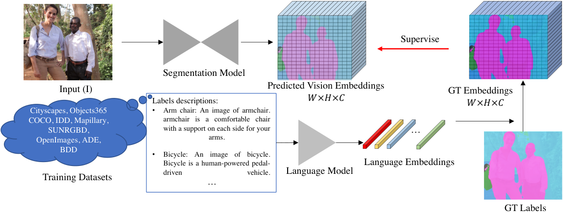
Figure 2 shows the overview of our method. Current semantic segmentation methods feed an RGB image to a neural network and predict per-pixel classes , where is the number of predetermined classes.
Recently, CLIP radford2021learning shows promising robustness by leveraging natural language supervision for image classification on a large-scale dataset. Inspired by this, instead of using one-hot vectors to represent the predefined labels, we employ language models to encode semantic labels into embedding vectors. In our experiments, we use the CLIP-ViT language model to encode all labels. The encoded language embeddings are , where is the embedding dimension. The vision embeddings from the segmentation model are .

Creating Language Embeddings. To train a robust model, we merged datasets together for training, containing labels in total. Lambert et al. MSeg_2020_CVPR manually create a unified label list and encode each label in a one-hot vector. All labels are independent to each other. In contrast, we employ a soft semantic embedding to replace the original labels, which can retain the relations among labels. Such relations are important for segmenting zero-shot labels.
Ideally, the closeness between embeddings is positively correlated to the similarity between different labels. For example, ‘Pedestrian’ should be close to ‘Rider’ but far from ‘Animals’ and other objects. Recently, several zero-shot semantic segmentation and classification methods bucher2019zerobaek2021exploitinghu2020uncertainty explore pre-trained linguistic semantic features using class names (i.e., word2vec). The problem is that words are sensitive to linguistic issues and can give little discriminability of classes. Some names may partially overlap or not well reflect semantic similarity. For example, ‘counter’ can be a counting device or a long flat-topped fitment. By contrast, textual descriptions are rich in context information. We thus collect short descriptions from Wikipedia to represent each label. For example, ‘bus: An image of bus. A bus is a road vehicle designed to carry many passengers.’ Figure 3 visualizes the cosine similarity matrix of embeddings, which are created from words or sentences. The block-diagonal nature demonstrates that our sentences embeddings better represent the semantic similarities. For example, classes in ‘Animals’ are close to each other but far from those in ‘People’.
Heterogeneous Constraints for Mixed Data Training. To obtain a robust segmentation model, we merge 9 datasets for training, including 7 well-annotated datasets, a coarsely-annotated dataset (OpenImages OpenImagesSegmentation), and a weakly annotated dataset (Objects365 shao2019objects365). Owing to the unbalanced quality, we propose to employ heterogeneous losses to train the model. For well annotated datasets, we enforce a pixel-wise loss on all samples. The loss function is as follows.
| (1) | ||||
| (2) | ||||
| (3) | ||||
where is the number of valid pixels, total categories, is the ground-truth labels, and is the learnable temperature. is the created language embeddings of training labels, while is the predicted vision embeddings.

As a coarsely annotated dataset contains many noises, we observe that directly enforcing the above pixel-wise loss leads to worse results. Figure 5 shows some noisy annotations from the OpenImages dataset. To alleviate the effect of such noises, we propose to enforce the loss on some high-confident samples and ignore the noisiest parts. The loss functions are as follows:
| (4) |
| (5) |
where is an adaptive threshold. In our experiments, we rank all samples’ losses of each image and set to the highest 30% loss value. Each image has an adaptive threshold. With the proposed heterogeneous loss for OpenImages, we can obtain much better segments (see Figure 7).
Furthermore, we propose a distillation method to leverage the weakly annotated dataset, Objects365, which only contains bounding boxes for foreground objects. Specially, since the CLIP classification model has obtained robust knowledge of image contents, we distill such knowledge to our segmentation model on box-level annotations.
We crop and resize the bounding box from the image and feed it to the CLIP classification model to obtain the vision embedding for objects, . is the image and is the bounding box. To retrieve the predicted bounding box embedding, we crop the corresponding region from the segmentation embeddings and enforce a convolution and ROI pooling on that . Lastly, we apply the loss to minimize their distance. The pipeline is shown in Figure 4.
| (6) | ||||
| (7) | ||||
where is the number of bounding boxes. The overall loss is as follows:
| (8) |
During inference, we calculate the cosine similarity between predicted vision embeddings and created language embeddings to obtain pixel-wise labels.
4 Experiments
4.1 Datasets and Implementation Details
In our experiments, we merged multiple datasets together for training and tested on 13 zero-shot datasets to evaluate the robustness of our method.
Training Data. We firstly merged 7 high-quality annotated semantic segmentation datasets (HD), including ADE20K zhou2017scene, Mapillary neuhold2017mapillary, COCO Panoptic lin2014microsoft, India Driving Dataset (IDD) varma2019idd, BDD100K (BDD) bdd100k, Cityscapes cordts2016cityscapes, and SUNRGBD song2015sun. Apart from that, we sample some data from the instance segmentation dataset OpenImagesV6 OpenImagesSegmentation (OI) and weakly annotated dataset Objects365 shao2019objects365 (OB) for training. Note that OpenImagesV6 only contains noisy foreground objects masks, while Objects365 provides objects bounding box annotations. These high-quality datasets (HD) have over 200K images. OpenImagesV6 has around 700K images, while Objects365 has over 1M images.
|
| ||||||
|---|---|---|---|---|---|---|---|
| CamVid brostow2008segmentation | Test set | Depth Estimation | |||||
| Pascal VOC everingham2015pascal | Validation set | NYUv2 | Test set | ||||
| Pascal Context mottaghi2014role | Validation set | KITTI | Test set | ||||
| KITTI Geiger2013IJRR | Test set | DIODE diode_dataset | Test set | ||||
| Wilddash1 zendel2018wilddash | Validation set | ScanNet dai2017scannet | Validation set | ||||
| Wilddash2 zendel2018wilddash | Test set | Sintel Butler:ECCV:2012 | Validation set | ||||
| Youtube VIS yang2019video | Sampled data | Instance Segmentation | |||||
| NYUv2 silberman2012indoor | Test set | COCO lin2014microsoft | Validation set | ||||

Testing Data for Semantic Segmentation. To evaluate the robustness and effectiveness of our semantic segmentation method, we test on 8 zero-shot datasets, including CamVid brostow2008segmentation, KITTI, Pascal VOC, Pascal Context, ScanNet dai2017scannet, WildDash1 zendel2018wilddash, WildDash2 zendel2018wilddash, YoutubeVIS yang2019video. Furthermore, we fine-tune our well-trained model on NYUv2 silberman2012indoor and Pascal Context to show our method can provide strong performance.
Testing Data for Downstream Applications. We create pseudo-semantic labels on zero-shot datasets to boost downstream applications, including instance segmentation and monocular depth estimation. We create pseudo instance masks on Objects365 to help instance segmentation on COCO lin2014microsoft. For depth estimation, following LeReS Wei2021CVPR, we create pseudo semantic masks on 9 RGBD datasets, of which 4 datasets are employed for training and others are for zero-shot depth evaluation, including NYUDv2, KITTI, DIODE diode_dataset, ScanNet, and Sintel Butler:ECCV:2012. More details are shown in Table 1.
| Methods | CamVid | KITTI | VOC | Pascal Context | ScanNet | WildDash1 | H-Mean |
|---|---|---|---|---|---|---|---|
| State-of-the-art methods on corresponding benchmarks | |||||||
| Zhu et al. zhu2019improving | 81.7 | - | - | - | - | - | - |
| Chroma UDA erkent2020semantic | - | 60.4 | - | - | - | - | - |
| AutoDeepLab liu2019auto | - | - | 82.0 | - | - | - | - |
| DeepLabV3+ chen2018encoder | - | - | - | 54.5 | - | - | - |
| Valada et al. valada2020self | - | - | - | - | 52.9 | - | - |
| HRNet trained on a single dataset, zero-shot testing | |||||||
| HRNet SunXLW19 (COCO) | 56.6 | 48.2 | 73.7 | 43.1 | 33.9 | 38.9 | 46.0 |
| HRNet (ADE) | 53.5 | 44.3 | 34.6 | 24.0 | 43.8 | 37.0 | 37.1 |
| HRNet (Mappilary) | 82.5 | 68.5 | 22.0 | 13.5 | 2.1 | 55.2 | 9.2 |
| HRNet (IDD) | 70.5 | 50.7 | 14.5 | 6.3 | 1.6 | 40.6 | 6.5 |
| HRNet (BDD) | 71.0 | 55.0 | 13.5 | 6.9 | 1.4 | 52.1 | 6.1 |
| HRNet (Cityscapes) | 65.3 | 58.1 | 12.1 | 6.5 | 1.7 | 30.1 | 6.7 |
| HRNet (SUN) | 0.1 | 0.7 | 10.2 | 4.3 | 42.2 | 1.4 | 0.3 |
| Methods trained on mixed datasets, zero-shot testing | |||||||
| MSeg MSeg_2020_CVPR | 82.4 | 62.4 | 70.8 | 45.2 | 48.4 | 64.2 | 59.6 |
| Ours_HRNet | 83.4 | 66.9 | 74.9 | 48.6 | 52.0 | 64.0 | 62.6 |
| Ours_Segformer | 83.7 | 68.9 | 81.1 | 54.2 | 55.3 | 69.7 | 66.9 |

Evaluation Metrics. We employ the mean intersection over union (mIoU) to evaluate semantic segmentation and AP lin2014microsoft for the instance segmentation. Following Ranftl2020Wei2021CVPR, we take absolute relative error (AbsRel) and percentage of pixels satisfying:
for evaluation. and are ground-truth and predicted depth respectively.
Multi-scale Evaluation for Semantic Segmentation. When evaluating the semantic segmentation performance, we employ multi-scale testing. We resize the testing images into multiple scales to feed into the model, i.e. with scales of 0.5 to 1.75 with 0.25 increments. Then we average the scores as the final prediction.
Implementation Details. We use two network architectures in our experiments, HRNet-W48 SunXLW19 and Segformer xie2021segformer. When training HRNet, we use SGD with momentum and polynomial learning rate decay, starting with a learning rate of 0.01. For the Segformer network, we use AdamW with polynomial learning rate decay and an initial learning rate 0.00006. To train a robust model on multiple datasets, following yin2021virtual, we balance all datasets in a mini-batch to ensure each dataset accounts for an almost equal ratio. During training, images from all datasets are resized such that their shorter edge is resized to 1080. We randomly crop the image by for HRNet and by for Segformer. Other data augmentation methods are also applied, including random flip, color transformations, image blur, and image corruption. In the inference, we resize the image with the short edge to one of three resolutions (4807201080). When comparing with existing methods, multi-scale (ms) or single-scale (ss) testing is employed.
| Methods | COCO | ADE | Mapillary | IDD | BDD | Cityscapes | SUN | H-Mean |
|---|---|---|---|---|---|---|---|---|
| Mseg | 48.6 | 42.8 | 51.9 | 61.8 | 63.5 | 76.3 | 46.1 | 53.9 |
| Ours_HRNet | 53.3 | 48.4 | 55.3 | 65.0 | 69.0 | 79.2 | 50.5 | 58.4 |
| Ours_Segformer | 64.6 | 55.1 | 59.1 | 67.0 | 70.5 | 82.9 | 50.5 | 62.8 |
| mIoU | |
|---|---|
| Mseg MSeg_2020_CVPR | 34.6 |
| Porzi Porzi_2019_CVPR | 37.1 |
| Ours | 37.9 |
4.2 Semantic Segmentation Evaluation
To demonstrate the robustness and effectiveness of our methods, we conduct evaluation on 15 datasets.
| Methods | Arch. | Training Data | CamVid | KITTI | VOC | Pascal Context | ScanNet | Wildash1 |
|---|---|---|---|---|---|---|---|---|
| Ours | HRNet-W48 | HD | 82.8 | 63.8 | 71.6 | 45.8 | 46.3 | 63.4 |
| Ours | HRNet-W48 | HD+OB | 83.4 | 66.0 | 74.6 | 48.3 | 49.8 | 63.4 |
| Ours | HRNet-W48 | HD+OI | 83.4 | 66.9 | 74.9 | 48.6 | 52.0 | 64.0 |
| Ours | Segformer-B5 | HD | 83.6 | 66.5 | 79.9 | 53.0 | 53.0 | 68.2 |
| Ours | Segformer-B5 | HD+OI+OB | 83.7 | 68.9 | 81.1 | 54.2 | 55.3 | 69.7 |
Robustness Evaluation. To show the robustness of our method, we firstly compare with existing state-of-the-art methods on 6 zero-shot datasets (unseen to our method during training). Note that current methods have been trained on testing datasets. Results are shown in Table 2. Our method can achieve state-of-the-art performance on CamViD, ScanNet, and WildDash1. Besides, we list the performance of HRNet SunXLW19 trained on an individual training dataset. We can see that our method, trained on mixed datasets, shows much better robustness than them. Furthermore, Mseg MSeg_2020_CVPR laboriously merged 7 well-annotated datasets and craftily designed a unified taxonomy for labels mapping. It shows strong generalization over these zero-shot testing datasets. By contrast, our methods, using sentences to automatically establish the label’s closeness, achieves much better performance than them over all zero-shot testing data. Furthermore, we show the performance comparison on the validation set of training data in Table 4. Our well-trained model outperforms Mseg over all datasets.
Evaluation on Wilddash2. The Wilddash2 benchmark is intended for testing the robustness of models trained on other datasets, and does not provide a training set of its own. Our method achieves the state-of-the-art performance on it. Results are shown in Table 4.
Effectiveness of Aggregating Noisy and Weak annotations with Heterogeneous Losses. We propose the heterogeneous losses to supervise the merged datasets. When aggregating OpenImages (‘HD+OI’) supervised with our , Table 5 shows the performance can be improved consistently over all zero-shot datasets. Figure 7 qualitatively compares with or without supervision for OpenImages (OI). We collect several web images for evaluation. We can observe that without loss (‘HD () + OI ()’), the predicted segments are much worse. Furthermore, when merging the Objects365 (OB) with the loss , the performance is improved over all zero-shot datasets.
| Method | Lizard | Shark | Frog | Deer | duck | Mean |
|---|---|---|---|---|---|---|
| mIoU (ss) | ||||||
| JoEm baek2021exploiting | 6.3 | 20.3 | 15.9 | 5.1 | 11.5 | 11.8 |
| Mseg MSeg_2020_CVPR | - | - | - | - | - | 17.3 |
| Ours (Word) | 13.1 | 11.2 | 11.1 | 4.2 | 22.8 | 12.5 |
| Ours (Sentence) | 23.6 | 51.6 | 25.8 | 17.8 | 36.1 | 31.0 |
Generalization on Unseen Labels. As we employ language embeddings to represent semantic labels, the visual similarity between labels are established by text expressions. In this experiment, we aim to observe if our resulting model can segment some zero-shot categories. Note that all these testing labels have never existed in our training data. We sampled around images with 5 zero-shot labels from YoutubeVIS Yang2019vis. Under this setting, we mainly compare with Mseg and JoEm baek2021exploiting because Mseg has strong generalization over cross domains and JoEm is the current state-of-the-art zero-shot semantic segmentation methods baek2021exploiting. We use their released weight for testing. JoEm is trained on the Pascal Context to segment 6 unseen classes. In contrast, as these labels are not in Mseg predetermined categories, we can only merge all their predicted animal labels to a single mask and evaluate the merged ’animal’ mask accuracy. We cannot retrieve any category information from its results. By contrast, ideally, our method and JoEm can segment these zero-shot labels, since we can encode descriptions of labels in language embeddings. By comparing the cosine similarity between predicted embeddings and language embeddings, the semantic label can be retrieved. We compare two encoding methods: 1) encoding label words (‘Ours (Word)’) 2) encoding short descriptions (‘Ours (Sentence)’). Results are illustrated in Table 6. Our method is more robust and can achieve better performance than JoEm and Mseg. Furthermore, we can observe that using sentences can achieve much better performance.
Finetuning on Small Datasets. In this experiment, we fine-tune our model on small datasets to show our well-trained weight can boost the performance significantly. We compare our well-trained weights, HRNet-W48 and Segformer-B5, with other weights on NYUv2 silberman2012indoor and Pascal Context mottaghi2014role. We fine-tune the model for 100 epochs on NYU and 50 epochs on Pascal Context. Quantitative comparisons are shown in Table 8. Compared with ImageNet pre-trained weight ‘*(ImageNet)’, our method surpasses them by a large margin, over 5% higher. Similarly, our method is better than Mseg and ADE20K pretrained weight (‘*(Mseg)’, ‘*(ADE20K)’). Compared with state-of-the-art methods, our method can achieve much better performance.
Effectiveness of Distillation. To employ large-scale weakly annotated data (Object365), we propose to use CLIP to distill our model. The experiment results are reported in Tab. 5. ‘HRNet-W48 HD’ is the baseline, which trains the model on large-scale high-quality semantic segmentation data. ‘HRNet-W48 HD+OB’ merge the segmentation data with object detection data (Object365). Although we only roughly distill the knowledge on cropped bounding box regions, the performance can still achieve noticeable improvement. We hypothesize the gains come from the large-scale Object365 data and CLIP’s strong and robust semantic knowledge.
Effectiveness of Merging Training Data with Language Embeddings. How to merge training data labels is important for mixed data training. In this ablation, we compare two different approaches to solve this problem. The baseline method is to naively merge all data labels and employ a cross-entropy loss to supervise the training, see ‘Naive Merge’ in Tab. 7. We can observe that the performance on zero-shot datasets is much worse than that of Mseg, which proposes a unified taxonomy for manually mapping labels. In contrast, we propose to employ sentence embeddings to represent labels. As the sentence embeddings can represent the underlying semantic similarities between classes, which is more applicable to solving label conflicts. Our method can achieve better performance than others.
| VOC | PC | CamVid | WildDash 1 | KITTI | ScanNet | |
|---|---|---|---|---|---|---|
| Naive Merge | 17.8 | 19.4 | 56.3 | 55.9 | 61.6 | 45.6 |
| Human Effort | 70.8 | 45.2 | 82.4 | 64.2 | 62.4 | 48.4 |
| Ours | 74.9 | 48.6 | 83.4 | 64 | 66.9 | 52 |
Comparison with Lseg The co-existing approach, Lseg li2022languagedriven, proposes a solution to perform zero-shot semantic segmentation by incorporating CLIP feature in their pipeline. In contrast, our method employs CLIP to create soft embeddings for sentences, allowing us to address the mixed-data taxonomy and enhance the model’s ability to generalize to zero-shot domains and labels by scaling up the training data. A quantitative comparison is presented in Fig. 8, where the model is evaluated on different label sets with varying levels of granularity. While both methods demonstrate comparable performance on coarse labels, our approach produces superior segmentation results on refined labels.

| NYUDV2 | Pascal Context | ||
|---|---|---|---|
| mIoU (ss) | |||
| MTI-Net vandenhende2020mti | 49.0 | OCR yuan2020object | 59.6 |
| ICM shi2019scene | 50.7 | CAA huang2021channelized | 60.5 |
| ShapeConv cao2021shapeconv | 51.3 | DPT ranftl2021vision | 60.5 |
| HRNet (ImageNet) | 44.5 | HRNet SunXLW19 | 50.3 |
| HRNet (Mseg) | 53.4 | HRNet (Mseg) | 52.6 |
| HRNet (Ours) | 54.1 | HRNet (Ours) | 52.8 |
| Segformer (ImageNet) | 50.0 | Segformer (ImageNet) | 59.4 |
| Segformer (ADE20K) | 59.1 | Segformer (ADE20K) | 60.8 |
| Segformer (Ours) | 60.0 | Segformer (Ours) | 65.0 |
| Method | Backbone | NYU | KITTI | DIODE | ScanNet | Sintel | |||||
|---|---|---|---|---|---|---|---|---|---|---|---|
| AbsRel | AbsRel | AbsRel | AbsRel | AbsRel | |||||||
| OASIS chen2020oasis | ResNet50 | ||||||||||
| MegaDepth li2018megadepth | Hourglass | ||||||||||
| Xian et al. xian2020structure | ResNet50 | ||||||||||
| DiverseDepth yin2020diversedepthyin2021virtual | ResNeXt50 | ||||||||||
| MiDaS Ranftl2020 | ResNeXt101 | ||||||||||
| LeReS Wei2021CVPR | ResNet50 | ||||||||||
| Ours LeReS | ResNet50 | 8.6 | 92.3 | 14.0 | 80.6 | 27.4 | 75.8 | 8.0 | 93.4 | 29.2 | 62.4 |
| Method | Backbone | Schedule | AP (%) | AP50 | AP75 | APS | APM | APL |
| Mask R-CNN he2017mask | R-50-FPN | 37.5 | 59.3 | 40.2 | 21.1 | 39.6 | 48.3 | |
| TensorMask chen2019tensormask | R-50-FPN | 35.4 | 57.2 | 37.3 | 16.3 | 36.8 | 49.3 | |
| BlendMask chen2020blendmask | R-50-FPN | 37.0 | 58.9 | 39.7 | 17.3 | 39.4 | 52.5 | |
| CondInst (10%COCO∗) | R-50-FPN | 21.7 | 35.2 | 22.0 | 8.9 | 22.4 | 31.1 | |
| Ours (CondInst), 10%COCO∗ | R-50-FPN | 33.2 | 52.1 | 35.2 | 15.0 | 36.4 | 48.0 | |
| CondInst (25%COCO∗) | R-50-FPN | 31.4 | 50.6 | 33.1 | 14.5 | 34.2 | 45.9 | |
| Ours (CondInst), 25%COCO∗ | R-50-FPN | 36.4 | 56.9 | 38.6 | 17.7 | 39.4 | 53.0 | |
| CondInst tian2020conditional | R-50-FPN | 35.9 | 57.0 | 38.2 | 19.0 | 40.3 | 48.7 | |
| Ours (CondInst), 50%COCO∗ | R-50-FPN | 38.1 | 59.0 | 40.8 | 18.7 | 41.5 | 55.2 | |
| Ours (CondInst), COCO | R-50-FPN | 39.5 | 60.7 | 42.5 | 19.5 | 42.9 | 57.5 | |
| Mask R-CNN | R-101-FPN | 38.3 | 61.2 | 40.8 | 18.2 | 40.6 | 54.1 | |
| PolarMask xie2020polarmask | R-101-FPN | 32.1 | 53.7 | 33.1 | 14.7 | 33.8 | 45.3 | |
| TensorMask | R-101-FPN | 37.1 | 59.3 | 39.4 | 17.4 | 39.1 | 51.6 | |
| BlendMask | R-101-FPN | 39.6 | 61.6 | 42.6 | 22.4 | 42.2 | 51.4 | |
| SOLOv2 wang2020solov2 | R-101-FPN | 39.7 | 60.7 | 42.9 | 17.3 | 42.9 | 57.4 | |
| CondInst | R-101-FPN | 40.0 | 62.0 | 42.9 | 21.4 | 42.6 | 53.0 | |
| CondInst | R-101-BiFPN | 40.5 | 62.4 | 43.4 | 21.8 | 43.3 | 53.3 | |
| Ours (CondInst) | R-101-BiFPN | 41.4 | 63.0 | 44.7 | 20.0 | 45.5 | 59.5 |
4.3 Boosting Downstream Applications
Boosting Monocular Depth Estimation. We create pseudo semantic labels on multiple zero-shot depth datasets to boost monocular depth estimation. Following LeReS Wei2021CVPR, we train monocular depth estimation model on Taskonomy zamir2018taskonomy, DIML kim2018deep, Holopix hua2020holopix50k, and HRWSI xian2020structure and evaluate it on 5 zero-shot datasets. On these 9 unseen datasets, we create pseudo semantic masks and transfer them to pixel-wise language embeddings, whose dimensions are 512. During training, we employ the ResNet50 backbone. The language embeddings are feed to a convolution to reduce the dimension from to , which is added to the depth prediction network. Then we add the transferred embeddings to the image feature after the first convolution. The framework is shown in Fig. 9. Results are shown in Table 9. Comparing with the baseline method ‘LeReS’, adding our created embeddings can consistently improve the performance over all datasets.
Boosting Instance Segmentation. Instance segmentation is another important fundamental problem. To demonstrate that our method can boost its performance, we create pseudo instance masks on sampled Objects365. The created pseudo labels have 7000K instance masks and 73 categories. We firstly train CondInst tian2020conditional on pseudo labels and then finetune it on COCO lin2014microsoft. Comparisons are illustrated in Table 10. With the ResNet-50 backbone, our method (‘Ours(CondInst), 25%COCO’), using only 25% COCO data, can achieve comparable performance with the baseline method ‘CondInst’, and can surpass other state-of-the-art methods with 50% COCO data. When finetuned on the whole COCO, our method is (‘Ours(CondInst), COCO’) around 4% AP higher than the baseline (‘CondInst’), and is even better than many methods with ResNet-101 backbone. We can observe that the main improvement comes from the medium () and large () objects.
5 Discussion
Limitations. We also observe a few limitations of our method. First, the performance of the model may be limited by the representation of the language model. Zero-shot categories with very similar semantic expressions may be confused. Second, the model may fail to generalize to classes that are too far from the training language space. However, we believe that if merging data with more categories in our method, we can achieve more distinguishable features and alleviate this problem. The improvement of the language model may also benefit the proposed method.
Conclusion. In this work, we have proposed an approach to semantic segmentation that can achieve promising performance over multiple zero-shot cross-domain datasets. By collecting short label descriptions from Wikipedia and encoding them in vector-valued embeddings to replace labels, we can easily merge multiple datasets together to retrieve a strong and robust segmentation model. A heterogeneous loss is proposed to leverage noisy datasets and weakly annotated datasets. Extensive experiments demonstrate that we can achieve better or comparable performance with current state-of-the-art methods on 7 cross-domain datasets. Furthermore, our resulting model demonstrates the ability to segment some zero-shot labels. With our robust and strong model, the downstream applications can also be boosted significantly.
Acknowledgements Part of this work was done when Wei Yin was an intern at Amazon.
References
- (1) N. Silberman, D. Hoiem, P. Kohli, and R. Fergus, “Indoor segmentation and support inference from rgbd images,” in Eur. Conf. Comput. Vis. Springer, 2012, pp. 746–760.
- (2) M. Everingham, S. A. Eslami, L. Van Gool, C. K. Williams, J. Winn, and A. Zisserman, “The pascal visual object classes challenge: A retrospective,” Int. J. Comput. Vis., vol. 111, no. 1, pp. 98–136, 2015.
- (3) M. Cordts, M. Omran, S. Ramos, T. Rehfeld, M. Enzweiler, R. Benenson, U. Franke, S. Roth, and B. Schiele, “The cityscapes dataset for semantic urban scene understanding,” in IEEE Conf. Comput. Vis. Pattern Recog., 2016, pp. 3213–3223.
- (4) T.-Y. Lin, M. Maire, S. Belongie, J. Hays, P. Perona, D. Ramanan, P. Dollár, and C. L. Zitnick, “Microsoft coco: Common objects in context,” in Eur. Conf. Comput. Vis. Springer, 2014, pp. 740–755.
- (5) Y. Xian, S. Choudhury, Y. He, B. Schiele, and Z. Akata, “Semantic projection network for zero-and few-label semantic segmentation,” in IEEE Conf. Comput. Vis. Pattern Recog., 2019, pp. 8256–8265.
- (6) P. Hu, S. Sclaroff, and K. Saenko, “Uncertainty-aware learning for zero-shot semantic segmentation.” Adv. Neural Inform. Process. Syst., vol. 3, p. 5, 2020.
- (7) D. Baek, Y. Oh, and B. Ham, “Exploiting a joint embedding space for generalized zero-shot semantic segmentation,” in Int. Conf. Comput. Vis., 2021, pp. 9536–9545.
- (8) H. Zhao, X. Puig, B. Zhou, S. Fidler, and A. Torralba, “Open vocabulary scene parsing,” in Int. Conf. Comput. Vis., 2017, pp. 2002–2010.
- (9) J. Lambert, Z. Liu, O. Sener, J. Hays, and V. Koltun, “MSeg: A composite dataset for multi-domain semantic segmentation,” in IEEE Conf. Comput. Vis. Pattern Recog., 2020.
- (10) A. Radford, J. W. Kim, C. Hallacy, A. Ramesh, G. Goh, S. Agarwal, G. Sastry, A. Askell, P. Mishkin, J. Clark et al., “Learning transferable visual models from natural language supervision,” arXiv: Comp. Res. Repository, p. 2103.00020, 2021.
- (11) R. Benenson, S. Popov, and V. Ferrari, “Large-scale interactive object segmentation with human annotators,” in IEEE Conf. Comput. Vis. Pattern Recog., 2019.
- (12) S. Shao, Z. Li, T. Zhang, C. Peng, G. Yu, X. Zhang, J. Li, and J. Sun, “Objects365: A large-scale, high-quality dataset for object detection,” in Int. Conf. Comput. Vis., 2019, pp. 8430–8439.
- (13) B. Li, K. Q. Weinberger, S. Belongie, V. Koltun, and R. Ranftl, “Language-driven semantic segmentation,” in Int. Conf. Learn. Represent., 2022.
- (14) J. Long, E. Shelhamer, and T. Darrell, “Fully convolutional networks for semantic segmentation,” in IEEE Conf. Comput. Vis. Pattern Recog., 2015, pp. 3431–3440.
- (15) E. Xie, W. Wang, Z. Yu, A. Anandkumar, J. M. Alvarez, and P. Luo, “SegFormer: Simple and efficient design for semantic segmentation with transformers,” Adv. Neural Inform. Process. Syst., 2021.
- (16) Z. Liu, Y. Lin, Y. Cao, H. Hu, Y. Wei, Z. Zhang, S. Lin, and B. Guo, “Swin transformer: Hierarchical vision transformer using shifted windows,” Int. Conf. Comput. Vis., 2021.
- (17) O. Zendel, K. Honauer, M. Murschitz, D. Steininger, and G. F. Dominguez, “Wilddash-creating hazard-aware benchmarks,” in Eur. Conf. Comput. Vis. Springer, 2018, pp. 402–416.
- (18) B. Cheng, A. G. Schwing, and A. Kirillov, “Per-pixel classification is not all you need for semantic segmentation,” 2021.
- (19) B. Cheng, I. Misra, A. G. Schwing, A. Kirillov, and R. Girdhar, “Masked-attention mask transformer for universal image segmentation,” 2022.
- (20) M. Bucher, T.-H. Vu, M. Cord, and P. Pérez, “Zero-shot semantic segmentation,” Adv. Neural Inform. Process. Syst., vol. 32, pp. 468–479, 2019.
- (21) Z. Gu, S. Zhou, L. Niu, Z. Zhao, and L. Zhang, “Context-aware feature generation for zero-shot semantic segmentation,” in ACM Int. Conf. Multimedia, 2020, pp. 1921–1929.
- (22) J. Ding, N. Xue, G.-S. Xia, and D. Dai, “Decoupling zero-shot semantic segmentation,” 2022.
- (23) G. A. Miller, “Wordnet: a lexical database for english,” Communications of the ACM, vol. 38, no. 11, pp. 39–41, 1995.
- (24) G. Ros, S. Stent, P. F. Alcantarilla, and T. Watanabe, “Training constrained deconvolutional networks for road scene semantic segmentation,” arXiv: Comp. Res. Repository, p. 1604.01545, 2016.
- (25) P. Bevandić, I. Krešo, M. Oršić, and S. Šegvić, “Simultaneous semantic segmentation and outlier detection in presence of domain shift,” in German Conf. Pattern Recogn. Springer, 2019, pp. 33–47.
- (26) K. Xian, C. Shen, Z. Cao, H. Lu, Y. Xiao, R. Li, and Z. Luo, “Monocular relative depth perception with web stereo data supervision,” in IEEE Conf. Comput. Vis. Pattern Recog., 2018, pp. 311–320.
- (27) W. Chen, Z. Fu, D. Yang, and J. Deng, “Single-image depth perception in the wild,” in Adv. Neural Inform. Process. Syst., 2016, pp. 730–738.
- (28) W. Yin, X. Wang, C. Shen, Y. Liu, Z. Tian, S. Xu, C. Sun, and D. Renyin, “Diversedepth: Affine-invariant depth prediction using diverse data,” arXiv: Comp. Res. Repository, p. 2002.00569, 2020.
- (29) W. Yin, C. Zhang, H. Chen, Z. Cai, G. Yu, K. Wang, X. Chen, and C. Shen, “Metric3d: Towards zero-shot metric 3d prediction from a single image,” Int. Conf. Comput. Vis., 2023.
- (30) W. Yin, J. Zhang, O. Wang, S. Niklaus, S. Chen, Y. Liu, and C. Shen, “Towards accurate reconstruction of 3d scene shape from a single monocular image,” IEEE Trans. Pattern Anal. Mach. Intell., 2022.
- (31) R. Ranftl, K. Lasinger, D. Hafner, K. Schindler, and V. Koltun, “Towards robust monocular depth estimation: Mixing datasets for zero-shot cross-dataset transfer,” IEEE Trans. Pattern Anal. Mach. Intell., 2020.
- (32) W. Yin, J. Zhang, O. Wang, S. Niklaus, L. Mai, S. Chen, and C. Shen, “Learning to recover 3d scene shape from a single image,” in IEEE Conf. Comput. Vis. Pattern Recog., 2021.
- (33) T. Mikolov, I. Sutskever, K. Chen, G. S. Corrado, and J. Dean, “Distributed representations of words and phrases and their compositionality,” in Adv. Neural Inform. Process. Syst., 2013, pp. 3111–3119.
- (34) S. Bujwid and J. Sullivan, “Large-scale zero-shot image classification from rich and diverse textual descriptions,” arXiv: Comp. Res. Repository, 2021.
- (35) B. Zhou, H. Zhao, X. Puig, S. Fidler, A. Barriuso, and A. Torralba, “Scene parsing through ade20k dataset,” in IEEE Conf. Comput. Vis. Pattern Recog., 2017.
- (36) G. Neuhold, T. Ollmann, S. Rota Bulo, and P. Kontschieder, “The mapillary vistas dataset for semantic understanding of street scenes,” in Int. Conf. Comput. Vis., 2017, pp. 4990–4999.
- (37) G. Varma, A. Subramanian, A. Namboodiri, M. Chandraker, and C. Jawahar, “Idd: A dataset for exploring problems of autonomous navigation in unconstrained environments,” in IEEE Winter Conf. on Applic. of Comp. Vis. IEEE, 2019, pp. 1743–1751.
- (38) F. Yu, H. Chen, X. Wang, W. Xian, Y. Chen, F. Liu, V. Madhavan, and T. Darrell, “Bdd100k: A diverse driving dataset for heterogeneous multitask learning,” in IEEE Conf. Comput. Vis. Pattern Recog., June 2020.
- (39) S. Song, S. P. Lichtenberg, and J. Xiao, “Sun rgb-d: A rgb-d scene understanding benchmark suite,” in IEEE Conf. Comput. Vis. Pattern Recog., 2015, pp. 567–576.
- (40) G. Brostow, J. Shotton, J. Fauqueur, and R. Cipolla, “Segmentation and recognition using structure from motion point clouds,” in Eur. Conf. Comput. Vis. Springer, 2008, pp. 44–57.
- (41) R. Mottaghi, X. Chen, X. Liu, N.-G. Cho, S.-W. Lee, S. Fidler, R. Urtasun, and A. Yuille, “The role of context for object detection and semantic segmentation in the wild,” in IEEE Conf. Comput. Vis. Pattern Recog., 2014, pp. 891–898.
- (42) A. Geiger, P. Lenz, C. Stiller, and R. Urtasun, “Vision meets robotics: The kitti dataset,” Int. J. of Rob. Research, 2013.
- (43) I. Vasiljevic, N. Kolkin, S. Zhang, R. Luo, H. Wang, F. Z. Dai, A. F. Daniele, M. Mostajabi, S. Basart, M. R. Walter, and G. Shakhnarovich, “DIODE: A Dense Indoor and Outdoor DEpth Dataset,” arXiv: Comp. Res. Repository, vol. 1908.00463, 2019. [Online]. Available: http://arxiv.org/abs/1908.00463
- (44) A. Dai, A. X. Chang, M. Savva, M. Halber, T. Funkhouser, and M. Nießner, “Scannet: Richly-annotated 3d reconstructions of indoor scenes,” in IEEE Conf. Comput. Vis. Pattern Recog., 2017, pp. 5828–5839.
- (45) D. J. Butler, J. Wulff, G. B. Stanley, and M. J. Black, “A naturalistic open source movie for optical flow evaluation,” in Eur. Conf. Comput. Vis., 2012, pp. 611–625.
- (46) L. Yang, Y. Fan, and N. Xu, “Video instance segmentation,” in Int. Conf. Comput. Vis., 2019, pp. 5188–5197.
- (47) Y. Zhu, K. Sapra, F. A. Reda, K. J. Shih, S. Newsam, A. Tao, and B. Catanzaro, “Improving semantic segmentation via video propagation and label relaxation,” in IEEE Conf. Comput. Vis. Pattern Recog., 2019, pp. 8856–8865.
- (48) Ö. Erkent and C. Laugier, “Semantic segmentation with unsupervised domain adaptation under varying weather conditions for autonomous vehicles,” IEEE Robotics and Automation Letters, vol. 5, no. 2, pp. 3580–3587, 2020.
- (49) C. Liu, L.-C. Chen, F. Schroff, H. Adam, W. Hua, A. L. Yuille, and L. Fei-Fei, “Auto-deeplab: Hierarchical neural architecture search for semantic image segmentation,” in IEEE Conf. Comput. Vis. Pattern Recog., 2019, pp. 82–92.
- (50) L.-C. Chen, Y. Zhu, G. Papandreou, F. Schroff, and H. Adam, “Encoder-decoder with atrous separable convolution for semantic image segmentation,” in Eur. Conf. Comput. Vis. Springer, 2018, pp. 801–818.
- (51) A. Valada, R. Mohan, and W. Burgard, “Self-supervised model adaptation for multimodal semantic segmentation,” Int. J. Comput. Vis., vol. 128, no. 5, pp. 1239–1285, 2020.
- (52) K. Sun, B. Xiao, D. Liu, and J. Wang, “Deep high-resolution representation learning for human pose estimation,” in IEEE Conf. Comput. Vis. Pattern Recog., 2019.
- (53) W. Yin, Y. Liu, and C. Shen, “Virtual normal: Enforcing geometric constraints for accurate and robust depth prediction,” IEEE Transactions on Pattern Analysis and Machine Intelligence (TPAMI), 2021.
- (54) L. Porzi, S. Rota Bulò, A. Colovic, and P. Kontschieder, “Seamless scene segmentation,” in IEEE Conf. Comput. Vis. Pattern Recog., June 2019.
- (55) L. Yang, Y. Fan, and N. Xu, “Video instance segmentation,” arXiv: Comp. Res. Repository, vol. 1905.04804, 2019. [Online]. Available: https://arxiv.org/abs/1905.04804
- (56) S. Vandenhende, S. Georgoulis, and L. Van Gool, “Mti-net: Multi-scale task interaction networks for multi-task learning,” in Eur. Conf. Comput. Vis. Springer, 2020, pp. 527–543.
- (57) Y. Yuan, X. Chen, and J. Wang, “Object-contextual representations for semantic segmentation,” in Eur. Conf. Comput. Vis. Springer, 2020, pp. 173–190.
- (58) H. Shi, H. Li, Q. Wu, and Z. Song, “Scene parsing via integrated classification model and variance-based regularization,” in IEEE Conf. Comput. Vis. Pattern Recog., 2019, pp. 5307–5316.
- (59) Y. Huang, W. Jia, X. He, L. Liu, Y. Li, and D. Tao, “Channelized axial attention for semantic segmentation,” arXiv: Comp. Res. Repository, p. 2101.07434, 2021.
- (60) J. Cao, H. Leng, D. Lischinski, D. Cohen-Or, C. Tu, and Y. Li, “Shapeconv: Shape-aware convolutional layer for indoor rgb-d semantic segmentation,” arXiv: Comp. Res. Repository, p. 2108.10528, 2021.
- (61) R. Ranftl, A. Bochkovskiy, and V. Koltun, “Vision transformers for dense prediction,” in Int. Conf. Comput. Vis., 2021, pp. 12 179–12 188.
- (62) W. Chen, S. Qian, D. Fan, N. Kojima, M. Hamilton, and J. Deng, “Oasis: A large-scale dataset for single image 3d in the wild,” in IEEE Conf. Comput. Vis. Pattern Recog., 2020, pp. 679–688.
- (63) Z. Li and N. Snavely, “Megadepth: Learning single-view depth prediction from internet photos,” in IEEE Conf. Comput. Vis. Pattern Recog., 2018, pp. 2041–2050.
- (64) K. Xian, J. Zhang, O. Wang, L. Mai, Z. Lin, and Z. Cao, “Structure-guided ranking loss for single image depth prediction,” in IEEE Conf. Comput. Vis. Pattern Recog., 2020, pp. 611–620.
- (65) K. He, G. Gkioxari, P. Dollár, and R. Girshick, “Mask r-cnn,” in Int. Conf. Comput. Vis., 2017, pp. 2961–2969.
- (66) X. Chen, R. Girshick, K. He, and P. Dollár, “Tensormask: A foundation for dense object segmentation,” in Int. Conf. Comput. Vis., 2019, pp. 2061–2069.
- (67) H. Chen, K. Sun, Z. Tian, C. Shen, Y. Huang, and Y. Yan, “BlendMask: Top-down meets bottom-up for instance segmentation,” in IEEE Conf. Comput. Vis. Pattern Recog., 2020.
- (68) Z. Tian, C. Shen, and H. Chen, “Conditional convolutions for instance segmentation,” in Eur. Conf. Comput. Vis. Springer, 2020.
- (69) E. Xie, P. Sun, X. Song, W. Wang, X. Liu, D. Liang, C. Shen, and P. Luo, “Polarmask: Single shot instance segmentation with polar representation,” in IEEE Conf. Comput. Vis. Pattern Recog., 2020, pp. 12 193–12 202.
- (70) X. Wang, R. Zhang, T. Kong, L. Li, and C. Shen, “SOLOv2: Dynamic and fast instance segmentation,” in Adv. Neural Inform. Process. Syst., 2020.
- (71) A. Zamir, A. Sax, , W. Shen, L. Guibas, J. Malik, and S. Savarese, “Taskonomy: Disentangling task transfer learning,” in IEEE Conf. Comput. Vis. Pattern Recog. IEEE, 2018.
- (72) Y. Kim, H. Jung, D. Min, and K. Sohn, “Deep monocular depth estimation via integration of global and local predictions,” IEEE Trans. Image Process., vol. 27, no. 8, pp. 4131–4144, 2018.
- (73) Y. Hua, P. Kohli, P. Uplavikar, A. Ravi, S. Gunaseelan, J. Orozco, and E. Li, “Holopix50k: A large-scale in-the-wild stereo image dataset,” in IEEE Conf. Comput. Vis. Pattern Recog. Worksh., June 2020.