Population Calibration using Likelihood-Free Bayesian Inference
Abstract
In this paper we develop a likelihood-free approach for population calibration, which involves finding distributions of model parameters when fed through the model produces a set of outputs that matches available population data. Unlike most other approaches to population calibration, our method produces uncertainty quantification on the estimated distribution. Furthermore, the method can be applied to any population calibration problem, regardless of whether the model of interest is deterministic or stochastic, or whether the population data is observed with or without measurement error. We demonstrate the method on several examples, including one with real data. We also discuss the computational limitations of the approach. Immediate applications for the methodology developed here exist in many areas of medical research including cancer, COVID-19, drug development and cardiology.
Keywords: approximate Bayesian computation, Bayesian synthetic likelihood, flow cytometry, heterogeneity, inter-subject variability, population of models
1 Introduction
In this paper we are interested in the problem of determining the distribution of inputs for a black-box function (deterministic or stochastic) that, when passed through this function, produces a distribution of outputs that ‘matches’ some target distribution. The most immediate use-case for this process is in calibrating a mathematical model to data that exhibits heterogeneity, where this heterogeneity is important. For example, it is insufficient to consider only the “mean” individual when analysing the absorption dynamics of a drug treatment (Rieger et al., 2018) or the potential for life-threatening side-effects (Passini et al., 2017). Instead, we wish to learn the spread of hidden model parameters across the whole population, as implied by the associated spread of measurable properties. Performing this calibration in a statistically rigorous way can be critical to learning population parameters that are actually representative of the true dynamics (Lawson et al., 2018).
Biological variability is exhibited at all levels of living organisms and readily captured by data (Britton et al., 2013). This data can be measurements which compare cell variability or differences in disease dynamics across the human population. For example, an individual’s cancer growth and treatment is extremely heterogeneous and this heterogeneity leads to the minimal success of most drugs at clinical trials (Burrell and Swanton, 2014; Fisher et al., 2013). The variability in human disease responses has also been evident in the COVID-19 pandemic, where hospitalised patient biomarkers illustrate the extensive variability in human immune responses to SARS-CoV-2 infection (Mathew et al., 2020; Lucas et al., 2020). With all this available data, it is crucial for a method to be developed that can learn model population parameters capturing the heterogeneity in the data so as to better inform decision making.
A variety of names have been given to this class of problem. Working in signal processing, Baggenstoss, 2017 calls it pdf projection. Practical approaches taken by more application-focused works refer to constructing virtual populations (Rieger et al., 2018; Brown et al., 2015; Fuertinger et al., 2018; Jenner et al., 2021a; Jenner et al., 2021b; Barish et al., 2017) or populations of models (Britton et al., 2013; Passini et al., 2017), owing to the intent to then carry out further computer experiments on those populations. Works in cell biology speak directly of identifying or estimating population heterogeneity (Hasenauer et al., 2011; Lambert et al., 2021). Here, we suggest that the term population calibration is suitable, highlighting that this is a calibration (inverse) problem, but one that respects the variability evident in a population. In Section 2, we formalise the problem of population calibration, and provide a short review of previous methodological approaches.
In general, the population calibration problem is ill-posed; that is, there are potentially an infinite number of input distributions that can match the output distribution, or perhaps none at all in the case of model misspecification. Predominantly, previous approaches to population calibration return only a single distribution, and do not attempt to quantify the uncertainty in their result. We suggest that uncertainty quantification is important in this context, as it can provide insight into the parameters of the model whose distribution is well constrained by the population data. The most related method to ours is Hasenauer et al., 2011, who also produce uncertainty quantification on the estimated input distribution using a similar approach. However, their method is developed for deterministic models with a known noise component.
The main contribution of this paper is to develop a general approach for population calibration (Section 3) that can, in principle, be applied in any context, including deterministic or stochastic models, and with or without extrinsic noise. Further, in the presence of a stochastic model, it need not have a tractable likelihood function. Crucially, our method quantifies the uncertainty in the estimated input distribution due to ill-posedness of the problem, and also a finite sample size of population data. Our approach exploits the framework of likelihood-free inference (Sisson et al., 2018), which was originally designed to perform, or approximate, standard Bayesian inference for a statistical model with an intractable likelihood function. We have previously applied our likelihood-free approach to a specific population calibration problem in flow cytometry (Browning et al., 2021), but here we formalise and generalise the method. By presenting our general framework, we also seek to bring to the attention of statisticians the population calibration problem and its sub-problems, some of which have been considered in the statistical literature but many others not. A further contribution is that we discuss in detail the limitations of the general approach throughout the results and discussion sections. In particular, our quest for uncertainty quantification significantly increases the computational complexity of the problem. We hope that this will inspire the development of new and more computationally efficient methods.
2 Background
The marginal distributions of two correlated random variables and are related by the law of total probability,
| (1) |
where and are their marginal distributions, and is the conditional density of given . In the context of this paper, defines the model with parameter ; for a deterministic function , the conditional density is where is the Dirac delta function, whereas for a stochastic model, is the conditional density of the model output given the parameter. The fundamental population calibration problem is to find , given and .
Equation (1) is the Fredholm equation of the first kind, and where can be evaluated pointwise for a given and , density deconvolution approaches may be used (see Crucinio et al., 2021 and references therein). These approaches are common in image processing (Lu et al., 2010) and have also been used, for example, to “undo” the stochastic delay between disease incidence and the observable event, death (Goldstein et al., 2009). The expectation maximisation approaches often taken here do not naturally address the ill-posedness of the problem, however, requiring convolution with smoothing kernels to avoid concentration of onto spikes (Crucinio et al., 2021).
Methods for population calibration of deterministic models have also proliferated separately, without acknowledgement of the connection to Fredholm equations. Some approaches, particularly in cardiac electrophysiology, simplify the problem by matching to ranges of the population data rather than their distribution (for example Britton et al., 2013; Passini et al., 2017). Brown et al., 2015 infer parameters characterising the response to trauma in a small experimentally-observed population responding, then create a virtual population of 10,000 by sampling uniformly over the resultant parameter ranges.
Efforts to statistically improve population calibration in these applied contexts have included capturing the distributional moments of the data (Tixier et al., 2017) or sampling from the data density then using a post-processing step to account for the missing volume factor that we discuss further below (Lawson et al., 2018). Allen et al., 2016 generate a virtual population using data for cholesterol measurements. Virtual individual parameters are sampled from plausible ranges and then the virtual patient was included in the virtual population with some probability based on the original data distribution.
Hasenauer et al., 2011 take a unique approach and represent the unknown distribution function as a finite mixture of overlapping kernel distributions (i.e., Gaussian), transforming the population calibration problem to an approximate high-dimensional inference problem. The primary advantage of this approach is that the samples from the output distribution can be drawn using importance sampling with the mixture weights. While this approach allows the uncertainty in inferences to be quantified through uncertainty in individual mixture weights, the approach suffers from the requirement to pre-specify the locations and variances of the kernel functions, which may be difficult to do for a moderate to large number of model parameters.
Several approaches have used the idea of entropy maximisation to regularise the population calibration problem’s ill-posedness (Tixier et al., 2017; Dixit et al., 2020). Maximising the entropy of avoids the artificial introduction of information beyond what the data (or prior) provides, and hence avoids the over-concentration of onto individual promising regions where others might also exist.
By observing that equation (1) can be written in reverse, and introducing a prior distribution to make the formulation more general, we have that
For a deterministic model , this then simplifies to
| (2) |
as separately observed by Baggenstoss, 2017 and Lambert et al., 2021. The term is a volume correction term akin to the Jacobian determinants seen for invertible transformations of random variables. This integration over the level sets of inspired the terminology in those works of “uniform manifold sampling”, and “contour Monte Carlo”, respectively. Baggenstoss, 2017 demonstrates that entropy maximisation can be achieved by choice of the prior according to an energy statistic (and notably, that a uniform prior naturally provides maximum entropy solutions for bounded ). Lambert et al., 2021 observe that the volume correction term can be approximated offline by repeatedly sampling from the -marginal of , and estimating the density based on the resultant values using non- or semi-parametric density estimation
So long as this density is sufficiently well-approximated, (2) can then be sampled from using any posterior sampling approach that requires only that the posterior be defined up to a normalisation factor.
Typically, one does not have in closed form, but instead a series of samples from which the density must be estimated. This does also offer a hierarchical formulation, assigning individual parameter values to each observation and then regularising the distribution of values across the population via appropriate choice of hyperprior (for example Alahakoon et al., 2021). This type of approach may regain a traditional likelihood for population calibration, but could drastically increase the dimensionality of the sampling problem for the general population calibration problem. This therefore does not seem to be a scalable approach, at least when the data can be reasonably treated as independently and identically distributed samples from some distribution . Furthermore, most approaches treat the estimated as being known, and hence do not account for the uncertainty due to sample size, which could be considerable if is small.
Several gaps remain in the literature surrounding population calibration. Although regularisation via entropy can help improve the single distribution obtained by these different approaches, almost all return only a single distribution, with no concept of the sensitivity or certainty of this result. This is a significant downside, as uncertainty arises both due to the ill-posedness of the problem and the reliance upon estimation of from a finite amount of data. Furthermore, most of the discussed approaches rely upon the model explicitly defining . In the approach we put forward here, one needs only to be able to sample from , and learns a distribution over distributions, unlocking the full benefits of the Bayesian paradigm for population calibration.
3 Likelihood-Free Bayesian Inference for Population Calibration
Here we describe our general population calibration approach, using the framework of likelihood-free inference. We first provide an overview of likelihood-free inference in the context of a more standard Bayesian calibration problem. We then show how the likelihood-free framework can be leveraged to solve the general population calibration problem, and importantly how it can produce uncertainty quantification on the estimated .
3.1 Likelihood-Free Bayesian Inference
For ease of exposition, we focus here on the popular methods of approximate Bayesian computation (ABC) and Bayesian synthetic likelihood (BSL). We note however that virtually any likelihood-free inference method could be considered for population calibration, and we refer to Sisson et al., 2018 and Cranmer et al., 2019 for a more comprehensive overview of statistical and machine learning approaches, respectively.
The goal of Bayesian inference is to estimate the posterior distribution of model parameters , in light of the prior distribution and the likelihood function for observed data, :
Likelihood-free inference methods have been developed for so-called implicit models, which are generative models that can be simulated but the corresponding likelihood function is computationally intractable and standard Bayesian inference approaches are thus ruled out. ABC proposes to target the following approximate posterior
| (3) |
where is a dataset simulated from the model at . Here, is a function measuring the distance between observed and simulated data, and is a threshold defining what is ‘close enough’, setting the indicator function to one when the simulated and observed data are sufficiently similar and zero otherwise. It is rather common, but not essential, to compute the distance between observed and simulated datasets on the basis of a carefully chosen summary statistic function so that becomes . The primary motivation for summarising the data is to avoid measuring closeness between large datasets, which may be difficult to do efficiently. However, comparing the empirical distribution of observed and simulated datasets can be effective, see Drovandi and Frazier, 2021 for a review of such approaches.
The integral in (3) can be estimated by Monte Carlo integration, drawing independent simulations of from for a given . Thus sampling of can proceed without ever evaluating . There exist a plethora of algorithms for approximate sampling of , with common sampling classes including, but not limited to, rejection (e.g. Beaumont et al., 2002), Markov chain Monte Carlo (MCMC, e.g. Marjoram et al., 2003) and sequential Monte Carlo (SMC, e.g. Sisson et al., 2007) sampling. The accuracy of ABC hinges on the informativeness of the observed data summarisation and the size of the tolerance , noting that further computational burden is often required to improve the approximation with respect to either of these two aspects (i.e. by increasing the dimension of or reducing ).
BSL is an alternative statistical approach for likelihood-free inference. Whereas ABC can be interpreted as using a non-parametric approximation of the summary statistic likelihood (Blum, 2010), BSL uses a parametric approximation. Specifically, Wood, 2010 proposes that
called the synthetic likelihood, where the mean and covariance may depend on the model parameter . Since such relationships are generally unknown, they are estimated empirically using sample moments calculated from the summary statistics of independent simulations of the model with parameter value . Price et al., 2018 examine the synthetic likelihood in the Bayesian framework. The estimated synthetic likelihood is often placed within an MCMC algorithm to sample the approximate posterior.
BSL has the advantage over ABC in terms of the number of tuning parameters; it requires specifying the number of simulated datasets for estimating synthetic likelihood, for which there is guidance in Price et al., 2018. Furthermore, it has been shown empirically (Price et al., 2018) and theoretically (Frazier et al., 2021b) that BSL scales more efficiently than ABC when the dimension of the summary statistic increases, at the expense of the Gaussian assumption. There are several extensions to BSL, such as a semi-parametric approach to relax the Gaussian assumption (An et al., 2020), whitening transformations of the summary statistic to reduce (Priddle et al., 2021) and handling model misspecification (Frazier and Drovandi, 2021). However, for simplicity, we only consider standard BSL in this paper.
3.2 Our Approach
We now provide details on how we can leverage the likelihood-free framework to solve population calibration problems, and simultaneously quantify the uncertainty in the solution. We first assume that the true belongs to a family of parametric distributions , parameterised by . We are interested in inferring , particularly via its posterior distribution in light of the population data and a prior distribution so that we can assess the uncertainty in the estimated . For example, if is the density function of a Gaussian distribution, then consists of a mean vector and covariance matrix, and the choice of prior might be something like a Gaussian-inverse-Wishart distribution. It may seem restrictive to only search within a given family of distributions, but we point out that such a choice also naturally introduces controllable regularisation to address the generally ill-posed nature of the population calibration problem. Posterior predictive checks can always be used to assess if the population data is well recovered, and if it is not, a more expressive family for can be considered. Domain expert knowledge could also be used to inform the choice of family for .
We note that there may be other parameters to estimate that are assumed to not vary between individuals. These may be parameters within the mathematical model (i.e. some components of ) that are assumed fixed for each individual or nuisance parameters such as the standard deviation of observation error. We denote these parameters as .
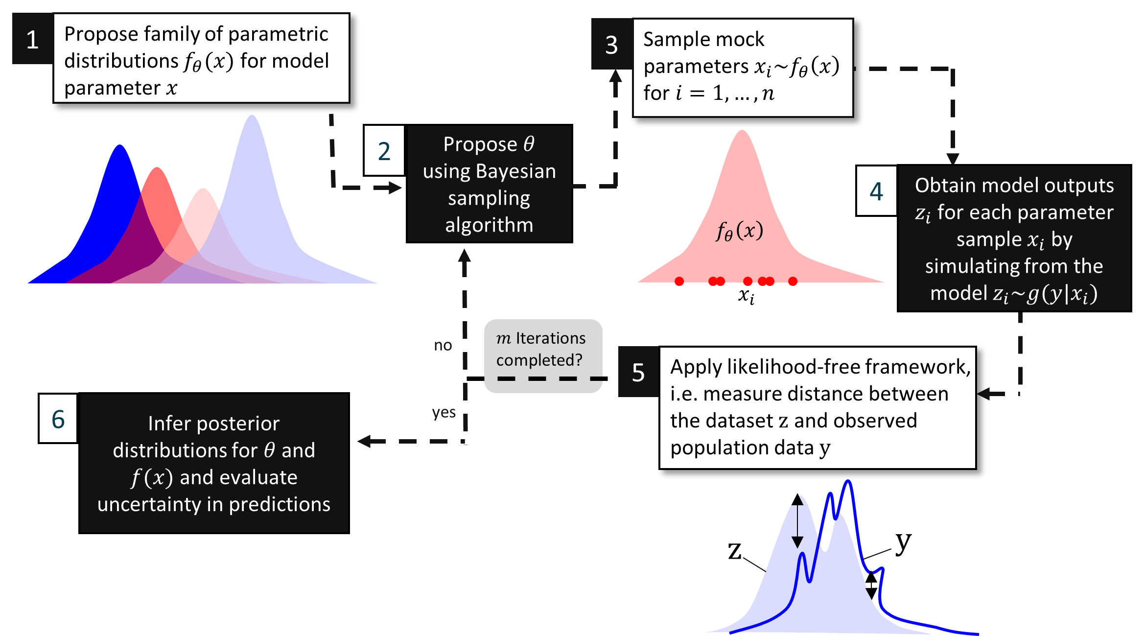
For a given value of proposed in a Bayesian sampling algorithm, we can simulate a mock population dataset by drawing and then simulating from the model, (or in the deterministic case) for such that . Then, all that is required to employ the likelihood-free framework is to devise an appropriate way to measure the distance between the datasets with in a distributional sense. That is to say, observations in each dataset are treated as unpaired and without ordering. For a summary of our approach see Figure 1.
There are several options for the comparison between and . If the population data is low-dimensional, then it would be feasible to construct a distance function for ABC by directly comparing the empirical distributions of and . Some such distances reviewed in Drovandi and Frazier, 2021 include the Wasserstein, Cramer von Mises and energy distances. For higher dimensional population data, it may be more efficient to work with features of the distribution, such as its location, scale and dependence. These summary statistics could be used in ABC, by choosing some appropriate distance function between summaries, or BSL. Regardless of the specific likelihood-free approach adopted, we compare simulated and observed datasets of the same size and we explicitly propagate the uncertainty due to final sample size through the estimation of . There is also flexibility with our approach. If there is no interest in accounting for uncertainty due to sample size it is possible to simulate datasets larger than the observed datasets. Conversely, if model simulation is expensive and the population data is large, then we can simulate less data than what was observed. We now illustrate our approach on a variety of population calibration problems.
4 Examples
Code to produce the results are available at
https://github.com/cdrovandi/Likelihood-Free-Population-Calibration.
4.1 Mixture model
Here we consider the Fredholm integration problem of the first kind from Ma, 2011 (also considered in Crucinio et al., 2021) with the following specifications:
which yields the output distribution
This is a de-noising problem, the goal being to recover the input distribution from the noise-corrupted output. Treating the noise corruption process as the model, however, it can also be interpreted as a population calibration problem for which both and have known, analytical expressions. As we go on to demonstrate, the significant amount of noise in this problem also acts to highlight its ill-posedness, and the importance of uncertainty quantification in this context.
We assume that observations have been drawn from to attempt to infer . As summary statistics we use the score of a two-component mixture of Gaussians, creating a five-dimensional summary statistic. We assume that the parametric form of is correctly specified. That is, it is specified as a two-component Gaussian mixture with to infer, where and are the mean and variance of the th component, and is the mixing weight for the first component. Our approach approximates the posterior of . For priors we use , and . In the prior we also impose the identifiability constraint that . We use iterations of BSL with to sample the approximate posterior of .
The results are shown in Figure 2. Figure 2(a) shows the univariate posterior distributions of with true values included. It is evident that is well-identified, except for where very small values are retained in the posterior. Figure 2(b) shows the posterior predictive distribution (specifically the median and 95% interval) of the estimated . Each prediction of is summarised by a kernel density estimate (KDE), which is also applied to the observed data. The median of the predicted KDEs is similar to the KDE of the observed data11 1 Strictly this point estimate is not a valid density estimate itself. Such a point estimate could be generated from a point estimate of or from finding the closest posterior KDE sample to the median point estimate.. Further, the 95% interval of the predicted KDEs tightly enclose the observed KDE. BSL is thus successful in finding combinations of that parametrically describe populations that exhibit the correct distribution of model output.
Figure 2(c) shows features of the posterior distribution of . A fair amount of uncertainty in is immediately seen, despite the close match to the output data across the posterior (Figure 2(b)). There is therefore a wide range of distributions that all represent populations that could have produced the observed data — the problem is indeed ill-posed. The uncertainty in comes mainly from the uncertainty in , for which very small values are permitted. This occurs because in the observed data, variability from the second mixture component and from the noisy model easily masks the effects of the first component’s small variance. Uncovering these aspects of a population calibration problem is only possible through approaches such as ours, that go beyond returning a single distribution as an answer. Of course, where a single answer is desirable, this is easily achieved once a posterior on distributions has been obtained — here, the median distribution is seen to agree well with the true population distribution. One could also choose the maximum entropy distribution from the posterior, so as to minimise any introduction of artificial knowledge (Tixier et al., 2017; Dixit et al., 2020).
4.2 Deterministic growth factor model
Here we consider population calibration for the deterministic growth factor model considered in Dixit et al., 2020 and Lambert et al., 2021. Consider the following coupled ordinary differential equations:
where and are the amount of ligand-free and ligand-bound receptors on the cell surface, respectively. The ligand is exogenously supplied, and its amount is treated as a fixed quantity, . We denote the model parameter as . Denote as the value of for a given and as found by forwards solution of the differential equation system. We consider a similar set-up to Lambert et al., 2021, fixing and drawing , . Bivariate population data is produced by observing the level of ligand-bound receptors for two different levels of ligand supply, across many different cells exhibiting the specified heterogeneity in parameters and . That is, we make independent draws of where denotes an independent replicate of . As noted in Lambert et al., 2021, the underlying population distribution can be approximated by a bivariate normal distribution with zero correlation.
We assume that samples are available from . We summarise the data with the two univariate sample means and variances, and the covariance between the two components, creating a five-dimensional summary statistic. For simplicity we denote these summaries as . We attempt to infer the underlying distributions of and that when pushed through the deterministic model can recapture the observed population data, or at least its features. We assume that distributions of and are correctly specified as independent Gaussians and we attempt to infer the means and standard deviations, . For the prior we use independent uniform distributions, , , , , which are specifications that are guided by Lambert et al., 2021 . We use 20000 iterations of MCMC BSL to infer the posterior distribution of .
The results are shown in Figure 3. Figure 3(a) shows the estimated univariate posterior distributions of . It can be seen that the components of are well identified, except for , which has a posterior distribution similar to its prior. Figure 3(b) shows, unsurprisingly, that the model is able to capture accurately the observed summary statistics of the population data. Features of the posterior distribution for the distribution of and throughout the population are shown in Figure 3(c). It is evident that the population distribution of is tightly constrained by the summaries of the population data. This is not surprising given the data is highly informative about the distribution’s mean and standard deviation (Figure 3(a)) The posterior median is close to the true distribution and the 95% CI closely envelopes the latter. In contrast, the population distribution of is not well identified from the population data. Even though the mean of is somewhat well identified, there is a great deal of uncertainty in its standard deviation (3(a)). This implies that a wide variety of distributions on can recover the summary statistics of the population data. Such distributions are shown in Figure 3(d).
Now we demonstrate how our method can be practically difficult to work with. Using the same dataset as above, we consider the same problem in Lambert et al., 2021 where the marginal population distribution of all five model parameters is calibrated. For our approach, now consists of 10 hyperparameters, . For the prior we use independent uniform distributions, , , , , , , , , , . If the data are informative enough, we should find that for , the estimated is close to the true parameter value and is estimated to be close to zero.
After several pilot runs to help inform the proposal distribution, we use 50000 iterations of MCMC BSL, producing trace plots as shown in Figure 4(a). It is evident that the MCMC has failed to converge. We find that the posterior distribution of is difficult to explore, with highly complex dependencies between hyperparameters a posteriori (results not shown). Despite this, Figure 4(b) shows that the model is capable of recovering the observed summary statistics of the data, and is very similar to Figure 3(b) for the two parameter problem. Trace plots for these summary statistics are also quite reasonable (results not shown). These results demonstrate that there are a huge variety of populations, differing in the nature of their heterogeneity, that all produce the observed variability in the data for ligand-bound receptor levels. This variety is further evident in Figure 4(c), where 10 randomly generated population distributions of the model parameters sampled from the MCMC chain are shown. The failure to converge truly highlights the hidden difficulty of population calibration problems for even deterministic models, especially when taking a fully Bayesian approach as we have done here. In such cases where the full population posterior is too difficult or expensive to appropriately explore, methods returning a single distribution that has been appropriately regularised do become more appealing. However, the approach of Lambert et al., 2021 to this problem significantly misspecifies the values (and distributions) of several of the model parameters, as compared to the true values used to generate the population data. An advantage of our approach is that it is able to quantify how informative a set of population data is.
4.3 Flow Cytometry
To demonstrate population calibration using real and potentially noisy experimental data, here we consider population variability in the internalisation of material by cells, where data are collected using flow cytometry (Browning et al., 2021). A distinguishing feature of this problem is the quantity of data available: flow cytometry provides single-cell information at rates exceeding several thousand cells per second (O’Neill et al., 2013), so our data comprise samples from several million cells (Browning et al., 2021). In the experiments, cells are incubated with fluorescent-labelled antibody that is internalised by transferrin receptors, the route usually reserved for the uptake of iron. The population calibration problem here is to infer distributional information relating to the variation in internalisation rates and cell size. We previously apply our approach to this population calibration problem in Browning et al., 2021 with code and data available at https://github.com/ap-browning/internalisation. The main focus of that paper is on the new biological insight that can be gained by considering population rather than averaged data. Here we focus mainly on the mathematical and statistical aspects of the problem, and refer to Browning et al., 2021 for more biological detail and motivation.
As the number of receptors and antibody molecules present on each cell is relatively large (), the transient dynamics can be modelled using the system of ODEs
| (4) |
Here, represents the relative number of internalised transferrin-bound receptors; that of antibody-bound receptors on the cell surface; that of antibody-bound receptors inside the cell; [] is the rate at which antibody-bound receptors are internalised; and, [] is the rate at which internalised receptors recycle to the cell surface. As the number of receptors present on each cell remains approximately constant, yet the fluorescent signal increases, we assume that a small proportion of internalised receptor-bound antibody, , disassociates and accumulates in a pool of free, internalised, antibody. All molecule counts are modelled as proportions of the total number of receptors present in each cell, and initially the system is assumed to be in an antibody-free equilibrium (Browning et al., 2021).
Flow cytometry (O’Neill et al., 2013) is used to collect noisy, single-cell, measurements relating to the amount of fluorescent material (i.e., antibody) present in each cell. To obtain information relating to both the total amount of antibody, and amount internalised on each cell, , antibody are labelled with two fluorescent probes, one of which can be selectively switched-off through the introduction of a quencher dye. Flow cytometry measurements typically comprise two sources of error: (1) circuit-derived noise, which can be modelled as Gaussian with variance proportional to the signal (Galbusera et al., 2020); and (2) cellular autofluorescence, or background fluorescence, which we model by constructing an empirical distribution using samples without antibody.
Measurements from each cell are, therefore, modelled by
Here, , where is the quenching efficiency; that is, the probability that the fluorescence of a surface-bound antibody molecule is switched off by the introduction of the quenched dye. is pre-estimated from the data; and are proportionality constants, relating the amount of fluorescent molecules to the magnitude of the flow cytometry signal; ; and, are jointly distributed random variables that represent cellular autofluorescence.
We capture cell-to-cell variability by modelling the number of receptors present in each cell, , the internalisation rate, , and the recycling rate, as jointly distributed random variables where here the subscript refers to the th cell. Without loss of generality, we set (i.e., receptor counts are relative to the population average). We assume that cell properties have a unimodal distribution and assume a parametric form of that allows us to infer the first three moments. The marginals are given by
| (8) | ||||
where and are shifted Gamma variables parameterised in terms of their respective means, standard deviations and skewnesses (negative skewness is allowed). Consistent with existing statistical modelling of flow cytometry data (Furusawa et al., 2005), is assumed to be log-normally distributed. To maintain positivity, we truncate all distributions so that (variables are parameterised in terms of the untruncated distributions). To allow for correlations between cell properties, we model the joint distribution of with a Gaussian copula with covariance matrix
| (9) |
Here, for such that remain positive definite.
Compared to the previous case studies, the internalisation model is heavily parameterised; and . We assume uniform priors (bounds correspond to the axis limits in Figure 5(a)) and infer the posterior distribution of using a hybrid SMC/MCMC ABC approach based on a discrepancy metric that matches a weighted sum of the correlations between measurements and , and the marginal distributions of each using the Anderson-Darling distance
| (10) |
where is the distribution function for the observed data and is the empirical distribution function of synthetically generated observations. For full details, see Browning et al., 2021. While the experimental data comprise cells per time point, quenched or not quenched, we simulate synthetic data sets based on (we treat this as a tuning parameter to balance computational burden and the ABC acceptance rate).
A major difficultly in the application of ABC is determining an appropriate acceptance tolerance. To address this, we first use an adaptive SMC ABC (Vo et al., 2015) algorithm to identify the region of the parameter space with non-negligible posterior density, and establish an achievable acceptance tolerance. We then choose an ABC acceptance tolerance based on the particle with the smallest discrepancy identified with SMC ABC having an acceptance rate of 50%. Next, we sample from the ABC posterior using 4 chains of iterations of MCMC ABC (Marjoram et al., 2003), thinning to every 10,000 samples. Posterior distributions are shown in Figure 5(a) and posterior predictive inputs are shown in Figure 5(b).
Despite the relatively large sample size, many parameters are practically non-identifiable. In particular, results for and indicate that model outputs are relatively insensitive to the shape of the internalisation and recycling rate distributions. However, we are able to identify that regions of the posterior where the internalisation rate is deterministic (i.e., ) have negligible support. Further, estimates for the proportion of receptors that recycle, , and estimates relating to the marginal distribution of (Figure 5(b)) are relatively constrained. Despite the lack of practical identifiability in , in Figure 6 we show that model predictions are relatively tightly constrained by producing posterior predictive distributions of the proportion of material internalised over the course of the experiment, a measurement that cannot be observed experimentally.
5 Discussion
In this paper we have presented a solution to the population calibration problem using likelihood-free inference. The advantages of the approach are that it can be applied, at least in principle, to any population calibration problem, and it produces uncertainty quantification on the estimated distribution of the model parameters. As illustrated in the paper, the main limitation is computational. Firstly, the approach requires a huge number of model solves or simulations. Secondly, the method requires sampling over the space of hyperparameters that may have a much larger dimension than the model parameters.
The most similar approach to ours (Hasenauer et al., 2011) uses in some sense a non-parametric approach where a mixture distribution with a relatively large number of components is used for where the hyperparameters of each component is fixed and only the mixture weights are inferred. This specification has the major advantage that model solves based on parameter values generated from the distribution of each mixture component can be generated and stored prior to running MCMC, and be recycled for different proposed mixture weights during MCMC. Their approach is designed for a deterministic model with known noise distribution, but could be adapted to a more general context. However, as the dimension of increases it is less clear how to set the hyperparameters of each mixture component. There may be other ways to recycle or exploit model solutions/simulations that have been generated offline or throughout the MCMC. For example, a surrogate model (Sacks et al., 1989) could be used to address the large number of forward simulations required by a fully Bayesian approach to population calibration if each is computationally costly. Even for problems too complex for construction of a sufficiently faithful surrogate, evaluations of the surrogate can still be incorporated into a sampling routine to improve proposals, and hence obtain speed-up without incurring any approximation error (Bon et al., 2021).
Another way to speed up the computations would be to replace MCMC with a variational approximation, which have been considered before in the likelihood-free literature (e.g. Tran et al., 2017; Ong et al., 2018). This approach would only provide an approximation to the posterior distribution of the hyperparameters, but still may provide valuable insight into the uncertainty quantification. We leave the exploration of more computationally efficient approaches for future research.
One potential issue that does not appear to have been addressed in the population calibration literature is model misspecification. Model misspecification in the context of population calibration could imply that there is no distribution on model parameters that can reproduce the population data. Fortunately, there has been some research in the likelihood-free literature for more standard Bayesian calibration in the presence of model misspecification, and the consequences that can arise (Frazier et al., 2020b; Frazier et al., 2021a). Frazier and Drovandi, 2021 extend BSL so that it can handle the situation where the model cannot reproduce all the summary statistics of the data, and can identify the offending summaries which can inform further model development. See Frazier et al., 2020a for an analogous approach to ABC. Such methods could be adapted to the population calibration context, but we leave that for further research.
Population calibration problems make up a growing proportion of the biological literature, as the need for mechanistic approaches to accommodate variability becomes better understood (see for example Brown et al., 2015; Fuertinger et al., 2018; Jenner et al., 2021a; Jenner et al., 2021b; Cassidy and Craig, 2019; Barish et al., 2017; Britton et al., 2013). In particular, virtual clinical trials (Alfonso et al., 2020) are becoming a popular way to examine an experimental treatment’s robustness before moving forward to clinical trial (Jenner et al., 2021a; Cassidy and Craig, 2019; Barish et al., 2017). Appropriate statistical treatment of these problems has been demonstrated to produce more predictive virtual populations, and to better distinguish parameter differences underlying separate cohorts in a dataset (Lawson et al., 2018). With the methodology presented here, these benefits now become available for models without an available likelihood, and we also gain a sense for the level of certainty in the population’s predicted variability. Our hope is that these methods be more widely applied to variable population data, such as flow cytometry measurements, genomic data, and survival curves, and also further developed to reduce the computational burden. Correctly capturing and characterising this variability, whether on the cellular level or the human level, is critical for these in silico studies to provide more reliable predictions and insights.
Acknowledgements
CD was supported by the Australian Research Council. ALJ was supported by a Queensland University of Technology Early Career Researcher Scheme. APB was supported by an ARC Centre of Excellence for Mathematical and Statistical Frontiers Research SPRINT scheme and an Australian Mathematical Society Lift-Off Fellowship.
References
- Alahakoon et al., (2021) Alahakoon, P., McCaw, J. M., and Taylor, P. G. (2021). Estimation of the probability of epidemic fade-out from multiple outbreak data. bioRxiv, page 446666.
- Alfonso et al., (2020) Alfonso, S., Jenner, A. L., and Craig, M. (2020). Translational approaches to treating dynamical diseases through in silico clinical trials. Chaos: An Interdisciplinary Journal of Nonlinear Science, 30(12):123128.
- Allen et al., (2016) Allen, R., Rieger, T. R., and Musante, C. J. (2016). Efficient generation and selection of virtual populations in quantitative systems pharmacology models. CPT: Pharmacometrics & Systems Pharmacology, 5(3):140–146.
- An et al., (2020) An, Z., Nott, D. J., and Drovandi, C. (2020). Robust Bayesian synthetic likelihood via a semi-parametric approach. Statistics and Computing, 30:543–557.
- Baggenstoss, (2017) Baggenstoss, P. M. (2017). Uniform manifold sampling (UMS): Sampling the maximum entropy PDF. IEEE Transactions on Signal Processing, 65(9):2455–2470.
- Barish et al., (2017) Barish, S., Ochs, M. F., Sontag, E. D., and Gevertz, J. L. (2017). Evaluating optimal therapy robustness by virtual expansion of a sample population, with a case study in cancer immunotherapy. Proceedings of the National Academy of Sciences, 114(31):E6277–E6286.
- Beaumont et al., (2002) Beaumont, M. A., Zhang, W., and Balding, D. J. (2002). Approximate Bayesian computation in population genetics. Genetics, 162(4):2025–2035.
- Blum, (2010) Blum, M. G. (2010). Approximate Bayesian computation: a nonparametric perspective. Journal of the American Statistical Association, 105(491):1178–1187.
- Bon et al., (2021) Bon, J. J., Lee, A., and Drovandi, C. C. (2021). Accelerating sequential Monte Carlo with surrogate likelihoods. Statistics and Computing, 31:62.
- Britton et al., (2013) Britton, O. J., Bueno-Orovio, A., Van Ammel, K., Lu, H. R., Towart, R., Gallacher, D. J., and Rodriguez, B. (2013). Experimentally calibrated population of models predicts and explains intersubject variability in cardiac cellular electrophysiology. Proceedings of the National Academy of Sciences, 110(23):E2098–E2105.
- Brown et al., (2015) Brown, D., Namas, R. A., Almahmoud, K., Zaaqoq, A., Sarkar, J., Barclay, D. A., Yin, J., Ghuma, A., Abboud, A., Constantine, G., et al. (2015). Trauma in silico: Individual-specific mathematical models and virtual clinical populations. Science Translational Medicine, 7(285):285ra61–285ra61.
- Browning et al., (2021) Browning, A. P., Ansari, N., Drovandi, C., Johnston, A., Simpson, M. J., and Jenner, A. L. (2021). Identifying cell-to-cell variability in internalisation using flow cytometry. bioRxiv.
- Burrell and Swanton, (2014) Burrell, R. A. and Swanton, C. (2014). Tumour heterogeneity and the evolution of polyclonal drug resistance. Molecular Oncology, 8(6):1095–1111.
- Cassidy and Craig, (2019) Cassidy, T. and Craig, M. (2019). Determinants of combination gm-csf immunotherapy and oncolytic virotherapy success identified through in silico treatment personalization. PLoS Computational Biology, 15(11):e1007495.
- Cranmer et al., (2019) Cranmer, K., Brehmer, J., and Louppe, G. (2019). The frontier of simulation-based inference. arXiv preprint arXiv:1911.01429.
- Crucinio et al., (2021) Crucinio, F. R., Doucet, A., and Johansen, A. M. (2021). A particle method for solving Fredholm equations of the first kind. Journal of the American Statistical Association, pages 1–11.
- Dixit et al., (2020) Dixit, P. D., Lyashenko, E., Niepel, M., and Vitkup, D. (2020). Maximum entropy framework for predictive inference of cell population heterogeneity and responses in signaling networks. Cell Systems, 10(2):204–212.
- Drovandi and Frazier, (2021) Drovandi, C. and Frazier, D. T. (2021). A comparison of likelihood-free methods with and without summary statistics. arXiv preprint arXiv:2103.02407.
- Fisher et al., (2013) Fisher, R., Pusztai, L., and Swanton, C. (2013). Cancer heterogeneity: implications for targeted therapeutics. British Journal of Cancer, 108(3):479–485.
- Frazier and Drovandi, (2021) Frazier, D. T. and Drovandi, C. (2021). Robust approximate Bayesian inference with synthetic likelihood. Journal of Computational and Graphical Statistics, pages 1–39.
- (21) Frazier, D. T., Drovandi, C., and Loaiza-Maya, R. (2020a). Robust approximate bayesian computation: An adjustment approach. arXiv preprint arXiv:2008.04099.
- (22) Frazier, D. T., Drovandi, C., and Nott, D. J. (2021a). Synthetic likelihood in misspecified models: Consequences and corrections. arXiv preprint arXiv:2104.03436.
- (23) Frazier, D. T., Nott, D. J., Drovandi, C., and Kohn, R. (2021b). Bayesian inference using synthetic likelihood: asymptotics and adjustments. arXiv preprint arXiv:1902.04827.
- (24) Frazier, D. T., Robert, C. P., and Rousseau, J. (2020b). Model misspecification in approximate Bayesian computation: consequences and diagnostics. Journal of the Royal Statistical Society: Series B (Statistical Methodology), 82(2):421–444.
- Fuertinger et al., (2018) Fuertinger, D. H., Topping, A., Kappel, F., Thijssen, S., and Kotanko, P. (2018). The virtual anemia trial: An assessment of model-based in silico clinical trials of anemia treatment algorithms in patients with hemodialysis. CPT: Pharmacometrics & Systems Pharmacology, 7(4):219–227.
- Furusawa et al., (2005) Furusawa, C., Suzuki, T., Kashiwagi, A., Yomo, T., and Kaneko, K. (2005). Ubiquity of log-normal distributions in intra-cellular reaction dynamics. Biophysics, 1:25–31.
- Galbusera et al., (2020) Galbusera, L., Bellement-Theroue, G., Urchueguia, A., Julou, T., and Nimwegen, E. v. (2020). Using fluorescence flow cytometry data for single-cell gene expression analysis in bacteria. PLOS ONE, 15(10):e0240233.
- Goldstein et al., (2009) Goldstein, E., Dushoff, J., Ma, J., Plotkin, J. B., Earn, D. J. D., and Lipsitch, M. (2009). Reconstructing influenza incidence by deconvolution of daily mortality time series. Proceedings of the National Academy of Sciences, 106(51):21825–21829.
- Hasenauer et al., (2011) Hasenauer, J., Waldherr, S., Doszczak, M., Radde, N., Scheurich, P., and Allgöwer, F. (2011). Identification of models of heterogeneous cell populations from population snapshot data. BMC Bioinformatics, 12(1):1–15.
- (30) Jenner, A. L., Aogo, R. A., Alfonso, S., Crowe, V., Deng, X., Smith, A. P., Morel, P. A., Davis, C. L., Smith, A. M., and Craig, M. (2021a). Covid-19 virtual patient cohort suggests immune mechanisms driving disease outcomes. PLoS Pathogens, 17(7):e1009753.
- (31) Jenner, A. L., Cassidy, T., Belaid, K., Bourgeois-Daigneault, M.-C., and Craig, M. (2021b). In silico trials predict that combination strategies for enhancing vesicular stomatitis oncolytic virus are determined by tumor aggressivity. Journal for Immunotherapy of Cancer, 9(2).
- Lambert et al., (2021) Lambert, B., Gavaghan, D. J., and Tavener, S. J. (2021). A Monte Carlo method to estimate cell population heterogeneity from cell snapshot data. Journal of Theoretical Biology, 511:110541.
- Lawson et al., (2018) Lawson, B. A. J., Drovandi, C. C., Cusimano, N., Burrage, P., Rodriguz, B., and Burrage, K. (2018). Unlocking data sets by calibrating populations of models to data density: A study in atrial electrophysiology. Science Advances, 4(1):1701676.
- Lu et al., (2010) Lu, Y., Shen, L., and Xu, Y. (2010). Integral equation models for image restoration: high accuracy methods and fast algorithms. Inverse Problems, 26:045006.
- Lucas et al., (2020) Lucas, C., Wong, P., Klein, J., Castro, T., Silva, J., Sundaram, M., Ellingson, M., Mao, T., Oh, J., Israelow, B., et al. (2020). Longitudinal immunological analyses reveal inflammatory misfiring in severe covid-19 patients. medRxiv.
- Ma, (2011) Ma, J. (2011). Indirect density estimation using the iterative Bayes algorithm. Computational Statistics & Data Analysis, 55(3):1180–1195.
- Marjoram et al., (2003) Marjoram, P., Molitor, J., Plagnol, V., and Tavare, S. (2003). Markov chain Monte Carlo without likelihoods. Proceedings of the National Academy of Sciences, 100(26):15324–15328.
- Mathew et al., (2020) Mathew, D., Giles, J. R., Baxter, A. E., Oldridge, D. A., Greenplate, A. R., Wu, J. E., Alanio, C., Kuri-Cervantes, L., Pampena, M. B., D’Andrea, K., et al. (2020). Deep immune profiling of covid-19 patients reveals distinct immunotypes with therapeutic implications. Science, 369(6508):eabc8511.
- O’Neill et al., (2013) O’Neill, K., Aghaeepour, N., Špidlen, J., and Brinkman, R. (2013). Flow cytometry bioinformatics. PLOS Computational Biology, 9(12):e1003365.
- Ong et al., (2018) Ong, V. M. H., Nott, D. J., Tran, M.-N., Sisson, S. A., and Drovandi, C. C. (2018). Variational Bayes with synthetic likelihood. Statistics and Computing, 28(4):971–988.
- Passini et al., (2017) Passini, E., Britton, O. J., Lu, H. R., Rohrbacher, J., Hermans, A. N., Gallacher, D. J., Greig, R. J. H., Bueno-Orovio, A., and Rodriguez, B. (2017). Human in silico drug trials demonstrate higher accuracy than animal models in predicting clinical pro-arrhythmic cardiotoxicity. Frontiers in Physiology, 8:668.
- Price et al., (2018) Price, L. F., Drovandi, C. C., Lee, A., and Nott, D. J. (2018). Bayesian synthetic likelihood. Journal of Computational and Graphical Statistics, 27(1):1–11.
- Priddle et al., (2021) Priddle, J. W., Sisson, S. A., Frazier, D. T., and Drovandi, C. (2021). Efficient Bayesian synthetic likelihood with whitening transformations. To appear in Journal of Computational and Graphical Statistics.
- Rieger et al., (2018) Rieger, T. R., Allen, R., Bystricky, L., Chen, Y., Colopy, G. W., Cui, Y., Gonzalez, A., Liu, Y., White, R. D., Everett, R. A., Banks, H. T., and Musante, C. J. (2018). Improving the generation and selection of virtual populations in quantitative systems pharmacology models. Progress in Biophysics & Molecular Biology, 139:15–22.
- Sacks et al., (1989) Sacks, J., Welch, W. J., Mitchell, T. J., and Wynn, H. P. (1989). Design and analysis of computer experiments. Statistical Science, 4:409–423.
- Sisson et al., (2018) Sisson, S. A., Fan, Y., and Beaumont, M. (2018). Handbook of Approximate Bayesian Computation. Chapman and Hall/CRC.
- Sisson et al., (2007) Sisson, S. A., Fan, Y., and Tanaka, M. M. (2007). Sequential Monte Carlo without likelihoods. Proceedings of the National Academy of Sciences, 104(6):1760–1765.
- Tixier et al., (2017) Tixier, E., Lombardi, D., Rodriguez, B., and Gerbeau, J.-F. (2017). Modelling variability in cardiac electrophysiology: a moment-matching approach. Journal of The Royal Society Interface, 14:20170238.
- Tran et al., (2017) Tran, M.-N., Nott, D. J., and Kohn, R. (2017). Variational Bayes with intractable likelihood. Journal of Computational and Graphical Statistics, 26(4):873–882.
- Vo et al., (2015) Vo, B. N., Drovandi, C. C., Pettitt, A. N., and Pettet, G. J. (2015). Melanoma cell colony expansion parameters revealed by approximate Bayesian computation. PLOS Computational Biology, 11(12):e1004635.
- Wood, (2010) Wood, S. N. (2010). Statistical inference for noisy nonlinear ecological dynamic systems. Nature, 466(7310):1102.