Flexible Triggering Kernels for Hawkes Process Modeling
Abstract
Recently proposed encoder-decoder structures for modeling Hawkes processes use transformer-inspired architectures, which encode the history of events via embeddings and self-attention mechanisms. These models deliver better prediction and goodness-of-fit than their RNN-based counterparts. However, they often require high computational and memory complexity requirements and sometimes fail to adequately capture the triggering function of the underlying process. So motivated, we introduce an efficient and general encoding of the historical event sequence by replacing the complex (multilayered) attention structures with triggering kernels of the observed data. Noting the similarity between the triggering kernels of a point process and the attention scores, we use a triggering kernel to replace the weights used to build history representations. Our estimate for the triggering function is equipped with a sigmoid gating mechanism that captures local-in-time triggering effects that are otherwise challenging with standard decaying-over-time kernels. Further, taking both event type representations and temporal embeddings as inputs, the model learns the underlying triggering type-time kernel parameters given pairs of event types. We present experiments on synthetic and real data sets widely used by competing models, while further including a COVID-19 dataset to illustrate a scenario where longitudinal covariates are available. Results show the proposed model outperforms existing approaches while being more efficient in terms of computational complexity and yielding interpretable results via direct application of the newly introduced kernel.
Keywords:
Machine Learning, ICML1 Introduction
Temporal point processes are the preferred choice when modeling asynchronous (irregularly sampled) event sequences (Cox & Isham 1980). Of particular interest is the Hawkes Process (Hawkes 1971), a self-exciting point process that has become popular and is used in numerous applications. In finance, the Hawkes process is used to model market return events, volatility, and market stability (Yang et al. 2018; Lee & Seo 2017; Bacry et al. 2015). In social media, it is employed to analyze malicious activity, and actions of users on social media platforms (Alvari & Shakarian 2019; Rizoiu et al. 2017). More recently, Hawkes processes have become critical in healthcare settings, such as modeling adverse drug reactions, disease progression, and spread of COVID-19 outbreaks (Bao et al. 2017; Chiang et al. 2021; Sun et al. 2021)
Hawkes 1971 first introduced the Hawkes process to model the aftershocks of earthquakes. The self-excitation mechanism allowed for modeling the clustered behavior of aftershock occurrences. Ozaki 1979 further introduced the likelihood function for the conditional intensity for the parametric estimation of the intensity function. Non-parametric approaches based on the expectation-maximization (EM) algorithm have also been proposed to estimate the conditional intensity function (Lewis & Mohler 2011; Chen & Hall 2016). However, these approaches suffer from expensive computational budgets needed to solve additional ordinary differential equation terms or the choice of the kernel functions needed to estimate the intensity function.
More recently, deep learning approaches have been introduced to model the event sequences with recurrent neural networks (RNNs) and attention-based architectures. Du et al. 2016 and Mei & Eisner 2017 model the intensity as a non-linear function of the sequence history by using RNNs to characterize the behavior of past events and feed-forward decoders to model the intensity function. These approaches aim to provide a flexible estimation of the conditional intensity function by avoiding strict assumptions on its functional form. However, the lack of a closed-form solution for the intensity function necessitates computationally expensive approximation techniques such as Monte Carlo to calculate the log-likelihood function values. Shchur et al. 2020 propose to replace the decoder used in the previous models with a log-normal mixture structure. By focusing on the conditional density function for the arrival times, they produce a closed-form solution for the expectation of the process. Their approach circumvents expensive approximations and yields efficient sampling of new sequences at the expense of assuming that all arrival times follow a log-normal distribution. Moreover, these models inherit the issues associated with RNNs, such as vanishing or exploding gradients (Pascanu et al. 2013), or the inability to capture long-term or very short-term dependencies (Zuo et al. 2020).
Attention-based models outperform their RNN counterparts because of their ability to capture dependencies irrespective of context length. Models with architectures similar to the transformer (Vaswani et al. 2017) encode the historical influence of past events with multiple attention layers and multiple attention heads. Zhang et al. 2020, and Zuo et al. 2020 introduced transformer-based approaches for Hawkes process modeling. These models create history embeddings based on a scoring function that compares the similarity of input vectors for each event in representation space. Though these attention-based structures can predict the arrival times relatively well, they suffer from high computational and memory requirements. Their results can be more interpretable compared to RNN-based approaches, but interpretability is limited to the relative contribution of past events. More importantly, these attention-based approaches struggle to infer the underlying intensity distribution of the point processes. The predefined attention score function, e.g., the exponentiated inner product, limits their ability to capture the triggering kernels of the point process. Besides, these models fail to differentiate between triggering kernels for various event type combinations, and do not consider (longitudinal) covariates into their modeling strategy.
Motivated to address the challenges faced by RNN- and attention-based approaches to the modeling of Hawkes processes, we propose a method that replaces the complex attention mechanisms with a more efficient, flexible, and interpretable encoding structure. Specifically, our approach replaces the attention mechanism with the direct estimation of the triggering kernels by taking advantage of the resemblance between the attention scores used to create the history embedding and the triggering function of the Hawkes process itself. The resulting encoder is more efficient than both RNNs and multi-layered attention structures, while being able to learn the triggering kernels of the underlying distribution directly from data. The proposed kernel uniquely combines a sigmoid gate (Steinruecken et al. 2019) with the rational quadratic function enabling the learning of a more general family of triggering kernels, such as local-in-time triggering, as well as the standard decaying-over-time functions. To our knowledge, this is the first approach that experiments with different structures to produce general triggering kernels geared toward point process modeling.
In addition to flexibility, the proposed sigmoid gated Hawkes process (SGHP) model can also learn a different triggering kernel for each pair of event types. Utilizing the event type embeddings previously used by existing attention-based models, we can readily estimate a triggering kernel for each event type combination while preventing the rapid growth of parameters, which typically scales with the square of the number of event types. Estimating kernels for each event type pairing allows one to interpret the effect of observing a given event type conditioned on other event types by examining their intensity function.
In order to showcase the flexibility, efficiency, and interpretability of the proposed model, we present experiments on both artificial and a wide range of real-world data; including comparisons with the state-of-art models. Results indicate that our model outperforms all the baseline models in terms of arrival time prediction and reproducing underlying triggering kernels, while being very competitive for event type prediction. Finally, we present results on a timely COVID-19 dataset of the patients admitted to the emergency department at [Name] Hospital and highlight the interpretability of our model via the learned triggering kernels for several event type pairings.
2 Background
Let be a sequence consisting of observed events (timestamps) from different possible event types. Each sequence can be represented as , where , and and correspond to the type and timestamp of an observed event, respectively. We use the subscript to represent an individual sequence, and and to denote events within a given sequence. Our objective is to model the underlying distribution of the collection of sequences for a given dataset of sequences, as well as predicting the arrival times and event types of future events conditioned on the history of past events.
2.1 Temporal Point Process
Temporal point processes are most often used to model the distribution of event sequences. Specifically, each temporal point process is characterized by its unique conditional intensity function , defined as
| (1) |
where is the history of previous events for , i.e., , is the conditional probability density function for the (next) event at time given the history of the sequence and is the corresponding conditional cumulative distribution function.
2.2 Hawkes Process
The Hawkes process (Hawkes 1971) is a special case of a temporal point process in which the intensity function is defined as follows
| (2) |
where is the exogenous background intensity and is the triggering kernel that allows the intensity function to depend on past events. Note that (2) is fully additive provided that both and are non-negative functions. Moreover, in some practical scenarios, the background intensity is assumed to be constant (Rasmussen & Williams 2005). Similarly, for the multivariate (multi-event) case
| (3) |
where represents the triggering kernel of an event of type on the current event type , and is the background intensity for type .
2.3 History Representations via Self Attention
Models based on self-attention have been proposed to capture the pairwise influence of all previous events in a sequence as a means to create historical representations (Zhang et al. 2020; Zuo et al. 2020). Specifically, the historical summary for event in the sequence is represented as follows
| (4) |
where is the latent vector (embedding) of the -th event in the sequence and is defined below, and is a similarity function usually specified as the exponentiated inner product between two embeddings, i.e.,
| (5) |
Note that other similarity functions are readily available and can be used in practice. However, (5) is still probably the most popular default choice.
2.4 Temporal Encoding
Attention-based models do not intrinsically capture (positional) information about the order of the events in a sequence like, for instance, RNN-based models do through recurrence. Zuo et al. 2020 introduced positional embeddings to account for such information into their encoding architecture. Further, Zhang et al. 2020 modified these embeddings for event sequences by incorporating event timestamps into the positional embeddings.
These modified positional embeddings, also know as temporal embeddings, are represented as for the -th event occurring at time . Assuming a temporal embedding in dimensions, each of its elements, , are defined as follows
| (6) |
where is defined as . Conceptually, represents the angular frequency of the -th dimension and is a scaling parameter that controls the weight of the time-shift and is learned from the data.
2.5 Event Type Embedding
To represent each event type in the sequence, a linear embedding layer is specified as in Zhang et al. 2020 via
| (7) |
where is a -dimensional (dense) vector representing the embedding for event at time , its one-hot encoding, and is the embedding matrix, and is also learned from data. Note that there are only distinct event type embeddings, which (in a slight abuse of notation) are indexed in (7) over time using the subscript .
3 Replacing Attention with a Kernel
Below we describe the proposed sigmoid gated kernel and explain the way in which we use it as a replacement for the attention mechanism in existing architectures (Zuo et al. 2020; Zhang et al. 2020).
3.1 Self Attention via the Triggering Function
We start by noting the similarity between the weights of the previous events for the attention mechanism in (2) obtained via , and the the triggering kernel in (3), for a conventional Hawkes process. Note that the triggering kernel captures the extent of the influence of past events, for , on the (future) event at time . Similarly, captures the influence of a past event on the future event , by proxy, leveraging representations and , for which we have , that encodes both temporal and event type information (Zhang et al. 2020). A significant difference is that in the standard Hawkes process, a triggering kernel is specified for each event-type pairwise combination, whereas in models based on the self-attention mechanism, such information is encapsulated in the event type embedding via (7). Alternatively, we propose to directly learn a flexible triggering kernel combinations for event types while still considering latent representations for the events in the history of events.
We now define the historical representation for the -th event in the sequence as follows
| (8) |
where is a triggering kernel like in the standard Hawkes processes defined in (3), one for each pair of event type combinations, and is the embedding of the -th event obtained as the concatenation of the event type and temporal embeddings, . Note that ) we concatenate the embeddings unlike in Zhang et al. 2020 to decouple the contribution of temporal and event type embeddings; in situations when longitudinal covariates are available, they can be readily incorporated as , where is the representation for the covariates at time (see Experiments for an example and Appendix B for details); and ) in (8) we need not to normalize the weights as in (4) because in (8), is meant to represent the aggregated, historical intensity rather than the average historical embedding.
Though for large values of it may seem inefficient to specify a triggering kernel for each combination, (8) allows for the behavior of each event type combination to be modeled separately over time, unlike implicitly done so in attention-based approaches. Below we will show that kernels for all event type combinations can be obtained efficiently by specifying a flexible kernel whose parameters are set and learned separately for each event type combination.

3.2 Flexible Kernel with Decay and Gating Effects
A natural choice for estimating a triggering function with a decaying effect over time is the squared exponential kernel, i.e., the radial basis function (RBF), which is widely used in machine learning applications such as kernel machines (Hearst et al. 1998) and Gaussian processes (Rasmussen & Williams 2005). Instead, we consider using the rational quadratic (RQ) kernel since it is a mixture of infinitely many squared exponential kernels, thus in principle, a more flexible yet easy to compute generalization of the squared exponential kernel (Rasmussen & Williams 2005). For a one dimensional process (with a single event type), the rational quadratic kernel is defined as follows
| (9) |
where and control the decay behavior, is the scaling parameter, and is a pairwise distance function, e.g., in (8).

The rational quadratic function is suitable to capture monotonically decaying effects, which are fairly standard in Hawkes processes. However, underlying triggering kernels in real-world point processes can be often more complex. As a particular example illustrated in Figure 1, consider a situation where the effect of a past event on the current event () does not decrease as the difference between event times grows but rather exhibits a localized behavior (at ) in which the effect is maximized at certain time difference (larger than zero). Such local effect is not possible to capture with regular decaying functions. To capture these local effects, we multiply the rational quadratic kernel with a sigmoid gate function, thus allowing the resulting kernel to capture both decay and local triggering effects. The proposed triggering kernel is then
| (10) |
where the first term is the rational quadratic kernel defined in (9), the second term is the generalized logistic function (Gupta & Kundu 2010), and . We modify the sigmoid function by adding the parameters and , which denote the location and rate of the change, respectively. As changes, the change-point moves across time, while s controls the spread of the change. Moreover, and still control the decay while is now the scaling parameter of the whole function. Figure 2 illustrates the behavior of (10) for different parameters choices and how the kernel flexibly models different triggering functions.
3.3 Efficient Learning of Event Type Kernel Pairs
Provided the triggering kernel function being able to capture decay and local effects as defined above in (10), we can proceed to generalize it for the multivariate (multi-event) process. Inconveniently, the number of parameters for the triggering kernels scales quadratically with the number of unique event types, , which may render the modeling prohibitive even for moderately large . Specifically kernel parameters scale with , where is the number of free parameters for the triggering kernel, i.e., in the proposed approach according to (10). For efficiency purposes, we estimate these parameters with feed-forward networks whose input are the concatenation of type embeddings as follows
| (11) |
where is the concatenation of embeddings for event types and , and is specified as a collection of individual fully connected networks via
| (12) |
where is a component of and . The mapping in (12) indicates that each parameter in has a corresponding weight vector and bias . As a result, kernel parameters scale linearly with and , i.e., , thus effectively removing their dependency on . Further, the non-negativity of the parameters is ensured by the softplus activation function. Note that one could also specify a single multilayer network for all parameters, however, in practice we found it more computational expensive but without substantial performance benefits.
4 Predicting for Next Event in the Sequence
The proposed model characterizes the underlying distribution of the point process by learning (temporal and event type) embeddings and the triggering kernels during the encoding stage. This allows for added flexibility in the decoder architecture. Specifically, by directly emphasizing on the prediction of next event (arrival) times and types during the decoding stage, we can encourage the predictive ability of the model. Further, we introduce stochasticity into the decoder to increase the variation (uncertainty) in the predictions and thus being able to approximate the predictive conditional distribution function for the arrival times.
4.1 Arrival Time Prediction
Given the historical embeddings for each time step, we can focus on predicting the next arrival time at each step. A straightforward way of obtaining arrival time predictions is to use a neural network whose input is the historical representation. We define such a feed-forward neural network as follows
| (13) |
Where is the encoded history vector defined in (8), and are the weight and bias of the feed-forward network, respectively. Note that stands for the arrival time prediction corresponding to event , and that we use the information (history representation) we have up to event to predict the arrival time for the next time step . The softplus activation is added to the output layer to ensure the arrival time predictions stay non-negative.
Adding Stochasticity to Predictions
As previously leveraged for generative models with adversarial learning (Goodfellow et al. 2014) (Mirza & Osindero 2014), we introduce stochasticity into our arrival time prediction by sampling noise vectors from an easy to sample distribution and adding them to the history representations. Specifically, the stochastic layer samples noise vectors of size from a uniform distribution. Each noise vector is passed through a linear layer before being added to , i.e.,
| (14) |
where is a sample from a uniform distribution, and and are specified accordingly to (13). The collection of samples can be thought as implicitly sampled from the desired predicted conditional distribution, i.e., .
Since the loss function (defined below) takes the predictions from all of these samples and updates the parameters of the model based on all of them, we are in principle able to approximate the conditional distribution of the arrival times. In practice, if distributional predictions are not a priority, we can simply summarize the -sample empirical distributions with sample characteristics such as mean, median or standard deviation. In the experiments, we use the sample mean as our final prediction for the arrival times.
4.2 Event Type Prediction
For multivariate event sequences, predicting the next event type is as important as predicting the arrival times. Unlike the models that use conditional intensity values of each event type, we can specify another feed-forward network that uses the history vectors as input to predict the event types directly. The event prediction is probabilistically defined as follows
| (15) |
where and are the weights and the bias of the feed-forward network, is the historical representation of event defined in (8), and , i.e., the output of the softmax function produces event type probabilities that can be converted into predicted event types for time .
4.3 Loss Function
We estimate the underlying distribution of the point process by learning the embeddings and triggering kernels, and use the next arrival times and event type as the target for the objective function. In addition to emphasize predictive ability, this allows us to avoid the integral approximations traditionally used in intensity-based decoders. (Zhang et al. 2020; Zuo et al. 2020; Shchur et al. 2020).
Since the decoders in (14) and (15) predict both the arrival times and event types, we ought to specify two different loss functions to train the model. Specifically, we use the loss for the arrival times and the cross-entropy loss for the event types. The complete loss is defined for the prediction of the next event at each observed timestamp as
where is a sample summary from (14), is the -th element of from (15) and is the ground truth indicator of whether time is of event type . Moreover, indicates that the loss is for a single sequence (preventing notation overload), and represents the set of all the parameters needed to be learned for the model. Precisely, the parameters of ) the triggering kernel parameter estimator in (11); ) the arrival time and event time predictors in (14) and (15), respectively; ) the scaling parameters of the temporal embeddings in (6); and ) the event type embeddings in (7). Finally, for the minimization problem we use the ADAM (Kingma & Ba 2015), provided it has proven to be computational efficient while requiring little parameter tuning compared to alternative algorithms.
5 Experiments
We present results on various synthetic and real-world datasets to compare the proposed sigmoid gated Hawkes process (SGHP) model against state-of-the-art Hawkes process models. Source code in Pytorch is available at https://github.com/yamacisik/gated_kernel_tpp.
5.1 Baseline Models
We consider two attention-based Hawkes process models (Zhang et al. 2020; Zuo et al. 2020) and an RNN-based log-normal mixture decoder model (Shchur et al. 2020). Further, we introduce a fourth baseline, namely, an attention-based log-normal mixture model, by replacing the RNN encoder in the original log-normal model with an attention encoder. We briefly describe the baseline models below.
Self Attentive Hawkes Process (SAHP): An attention-based model that uses multiple layers of multi-headed attention to model the intensity function based on historical embeddings. Zhang et al. 2020 introduced time-shifted positional embeddings to inject information on event time differences in addition to event temporal position. They learn the intensity function of the event sequence via maximum likelihood while using Monte Carlo sampling to approximate the cumulative intensity function.
Transformer Hawkes Process (THP): The model by Zuo et al. 2020 is a variant of an attention-based approach similar to SAHP. In addition to model the log-likelihood of the intensity function, they incorporate event time and type prediction losses for the training of their model. Like the SAHP model, the intensity function is a non-linear transformation of the base intensity with additive decay, thus the triggering kernels are not directly modeled.
Log-Normal Mixture Model (LMM): The log-normal mixture model (Shchur et al. 2020) is an intensity-free approach that models the conditional probability distribution of arrival time with a log-normal mixture model. The model uses an RNN to encode the history representations and the log-likelihood of the conditional event probabilities as their loss function, thus avoiding Monte Carlo sampling. However, to obtain the intensity function, they still need to approximate the integral of the cumulative distribution function.
LMM with Attention (LMMA): We replace the RNN decoding of the log-normal mixture model with an attention mechanism proposed in the SAHP model. This simple extension of LMM is introduced here to understand the performance of attention models with an intensity-free formulation. This is conceptually similar to our approach in that we summarize histories leveraging ideas from attention, but unlike other attention models, arrival event times and event types are predicted without the need to directly estimate the cumulative intensity function.
5.2 Datasets
We use a synthetic dataset sampled from a 2D Hawkes process and three real-word datasets previously used by the baseline models. Further, we consider a COVID-19 inpatient dataset collected at our Institution. Table 7 in the Appendix presents summary statistics for these datasets. With the exception of the COVID-19 dataset, all real-world datasets are publicly available (https://drive.google.com/drive/folders/1OB1Mcns6qvnkZ48MCnZbtvB9Rp5Dtfp6).
2D Hawkes (HP): We use the same 2D Hawkes dataset used by in the SAHP (Zhang et al. 2020). For reproducibility, we resampled the dataset from the tick library with a fixed random seed. Appendix A provides details on the triggering kernels and the baseline intensities used for the synthetic dataset.
Stackoverflow (SOF): The data set consists of users of the famous question-and-answer website Stack Overflow. Users get medals based on their questions or answers, e.g., good question, good answer, etc. Each user is modeled as a sequence with event types representing medals obtained over time.
Mimic-II (MMC): This electronic healthcare records dataset tracks the journey of patients through their hospital intensive care unit (ICU) stay over a period of seven years. Each patient sequence consists of timestamps and diagnoses for each visit.
Retweets (RT): The dataset tracks re-tweets made on particular tweets on the social media website Twitter. Every time a tweet is re-tweeted, the popularity of the re-tweeter and the timestamp of the retweet are recorded. There are three different re-tweeter categories based on their number of followers. Due to the wide range of the inter-arrival times, arrival time results are made relative by scaling over the maximum inter-arrival time.
COVID-19 Emergency Department (COVID): This dataset tracks the journey of COVID-19 patients admitted for patient care at [Name] Hospital Emergency Department (ED) between January of 2020 and December of 2021. We consider five different event types, namely, admission to ED for patient care, admission to ICU, admission to a step-down unit, discharge, and death. Further, the dataset also includes vitals measured between events. Specifically, five vitals: pulse oximetry (SpO2), mean arterial pressure (MAP), blood pressure (BP), temperature, and respiratory rate (RR).
6 Results
6.1 Capturing Triggering Kernels
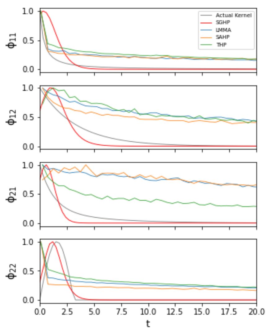
We present the estimated kernels for all the models against the ground-truth triggering functions for the synthetic data and compare the goodness-of-fit to the underlying distribution. Since our approach learns the parameters for each triggering kernel, we can plot the estimation directly as a function of time. For the attention-based models, we use the attention scores for each time difference observed in the data as proxy. We further split these scores across event type pairings. Moreover, to reduce the fluctuations in the attention-based scores, we pass them through a moving average filter where we take mean scores over a small time window (). Figure 3 shows the estimates for all models. As expected, the proposed gated kernel (SGHP) is the best match for all of the underlying triggering kernel pairings. Importantly, unlike the other models, it can accommodate to different event type pairings and capture both decaying and local effects.
| Dataset | LMM | LMMA | THP | SAHP | SGHP |
|---|---|---|---|---|---|
| HP | 2.25 | 2.23 | 2.42 | 2.29 | 2.11 |
| MMC | 0.88 | 0.80 | 0.859 | 0.821 | 0.79 |
| SOF | 1.46 | 1.49 | 1.66 | 1.55 | 1.30 |
| RT | 0.61 | 0.64 | 0.18 | 0.12 | 0.08 |
| COVID | 341.5 | 356.1 | 374.1 | 383.2 | 332.2 |
6.2 Sequence Prediction
Predicting the next event arrival time is a key objective when modeling event sequences. To capture the ability all models have to learn from the sequential event information, we report the event type and event time prediction results for the last observed event in each sequence. Specifically, we report (micro) F1 scores for event types, except for the COVID data for which a high class imbalance is observed, i.e., mortality. Instead, results for mortality prediction are provided below using average precision score as performance metric. For event arrival times, we report the mean squared error (RMSE). Tables 1 and 2 show RMSE and F1 scores, respectively, for the last event predictions in the test sets of all datasets and models being evaluated. In terms of RMSE, the proposed SGHP consistently outperforms the other approaches, while in terms of event type prediction, SGHP outperforms the others on the HP and RT datasets and delivers competitive results on MMC and SOF. Interestingly the best performing event type prediction model in MMC is LMMA, which is also introduced in this paper.
| Dataset | LMM | LMMA | THP | SAHP | SGHP |
|---|---|---|---|---|---|
| HP | 0.573 | 0.550 | 0.575 | 0.585 | 0.610 |
| MMC | 0.892 | 0.900 | 0.877 | 0.646 | 0.810 |
| SOF | 0.384 | 0.375 | 0.411 | 0.242 | 0.389 |
| RT | 0.544 | 0.528 | 0.539 | 0.531 | 0.605 |
6.3 Mortality Predictions for Covid-19 Patients
Complementing the real-world datasets in Table 2, we also seek to test the proposed model in a more realistic healthcare setting. Specifically, we compare models in terms of their ability to predict patient mortality. We treat the mortality prediction as a binary problem, e.g., death vs. survival. Since there is a significant class imbalance, we report the average precision score (APS) as opposed to F1 or area under the receiving operating characteristic (see Appendix for these). Moreover, we incorporate patient vitals as longitudinal covariates as a means to showcase that the model can readily process covariate information. Existing approaches do not consider covariates, but we have incorporated them as embeddings as described in Appendix B for fair comparison. Table 3 shows mortality prediction results on both variations of the COVID data (with and without vitals).Without covariates, SGHP delivers average performance while it outperforms the other approaches when longitudinal covariates (vitals) are included.
| Dataset | LMM | LMMA | THP | SAHP | SGHP |
|---|---|---|---|---|---|
| COVID | 0.18 | 0.16 | 0.07 | 0.004 | 0.12 |
| COVID+v | 0.12 | 0.21 | 0.1 | 0.005 | 0.22 |
6.4 Model Complexity
RNN-based and attention-based encoders tend to suffer from high complexity and memory requirements due to the large number of parameters that need to be estimated. Table 4 reports the total number of estimated parameters (in thousands) for each model across all the data sets. Note that all datasets use the same model architectures. We see that our model often requires a significantly smaller number of parameters for all prediction tasks, while delivering comparable or superior performance on both arrival times and event type prediction.
| Dataset | LMM | LMMA | THP | SAHP | SGHP |
|---|---|---|---|---|---|
| HP | 17.2 | 17.2 | 25.3 | 4.1 | 2.7 |
| MMC | 17.8 | 19.6 | 189 | 6.5 | 4.2 |
| SOF | 15.7 | 17.8 | 1595 | 4.8 | 3.7 |
| RT | 14.8 | 17.2 | 41.7 | 4.2 | 2.4 |
| COVID | 14.9 | 17.3 | 23.7 | 4.2 | 3.8 |
| Average | 16.9 | 17.8 | 417.8 | 4.8 | 3.1 |
6.5 Kernels Interpretation for COVID Data
Our model learns a triggering kernel for each event type pairing. This allows one to interpret the results in terms of intensity functions. Specifically, we report the likelihood of being admitted to ICU and mortality after observing that a patient is admitted to the ED, ICU, or a step-down unit. Figure 4 shows the learned triggering kernels for some of these possible transitions. As expected, the likelihood of mortality is by far sharper for patients already admitted to the ICU, relative to patients in ED beds or step-down units. Moreover, the likelihood of being admitted to the ICU is much higher for patients originating from a step-down unit.


7 Conclusion
We introduced a flexible, efficient, and interpretable approach for modeling Hawkes processes with an encoder-decoder structure. Our approach replaced the complex and more difficult to interpret attention mechanism with directly learning the underlying triggering kernels of the point processes. The proposed encoder uniquely combines a regular decaying kernel with a sigmoid gate, thus allowing it to capture a wide range of triggering functions otherwise not possible with other attention-based approaches. We further generalized our method for the multivariate Hawkes process and incorporated longitudinal covariates into the temporal process characterization. Finally, the experiments demonstrated that the proposed approach is superior to state-of-art methods in terms of predictive and computational performance, interpretation of the kernels learned from data.
References
- Alvari & Shakarian (2019) Alvari, H. and Shakarian, P. Hawkes process for understanding the influence of pathogenic social media accounts. In International Conference on Data Intelligence and Security, 2019.
- Bacry et al. (2015) Bacry, E., Mastromatteo, I., and Muzy, J.-F. Hawkes processes in finance. Market Microstructure and Liquidity, 2015.
- Bao et al. (2017) Bao, Y., Kuang, Z., Peissig, P., Page, D., and Willett, R. Hawkes process modeling of adverse drug reactions with longitudinal observational data. In Machine Learning for Healthcare Conference, 2017.
- Chen & Hall (2016) Chen, F. and Hall, P. Nonparametric estimation for self-exciting point processes—a parsimonious approach. Journal of Computational and Graphical Statistics, 2016.
- Chiang et al. (2021) Chiang, W.-H., Liu, X., and Mohler, G. Hawkes process modeling of covid-19 with mobility leading indicators and spatial covariates. International Journal of Forecasting, 2021.
- Cox & Isham (1980) Cox, D. and Isham, V. Point Processes. Chapman & Hall/CRC Monographs on Statistics & Applied Probability. Taylor & Francis, 1980.
- Du et al. (2016) Du, N., Dai, H., Trivedi, R., Upadhyay, U., Gomez-Rodriguez, M., and Song, L. Recurrent marked temporal point processes: Embedding event history to vector. In International Conference on Knowledge Discovery and Data Mining, 2016.
- Goodfellow et al. (2014) Goodfellow, I., Pouget-Abadie, J., Mirza, M., Xu, B., Warde-Farley, D., Ozair, S., Courville, A., and Bengio, Y. Generative adversarial nets. In Ghahramani, Z., Welling, M., Cortes, C., Lawrence, N., and Weinberger, K. Q. (eds.), Advances in Neural Information Processing Systems, 2014.
- Gupta & Kundu (2010) Gupta, R. D. and Kundu, D. Generalized logistic distributions. Journal of Applied Statistical Science, 2010.
- Hawkes (1971) Hawkes, A. G. Spectra of some self-exciting and mutually exciting. Biometrika, 1971.
- Hearst et al. (1998) Hearst, M., Dumais, S., Osuna, E., Platt, J., and Scholkopf, B. Support vector machines. IEEE Intelligent Systems and their Applications, 1998.
- Kingma & Ba (2015) Kingma, D. P. and Ba, J. Adam: A method for stochastic optimization. In International Conference on Learning Representations, 2015.
- Lee & Seo (2017) Lee, K. and Seo, B. K. Marked hawkes process modeling of price dynamics and volatility estimation. Journal of Empirical Finance, 2017.
- Lewis & Mohler (2011) Lewis, E. and Mohler, G. A nonparametric em algorithm for multiscale hawkes processes. Journal of Nonparametric Statistics, 2011.
- Mei & Eisner (2017) Mei, H. and Eisner, J. M. The neural hawkes process: A neurally self-modulating multivariate point process. In Advances in Neural Information Processing Systems, 2017.
- Mirza & Osindero (2014) Mirza, M. and Osindero, S. Conditional generative adversarial nets. CoRR, 2014.
- Ozaki (1979) Ozaki, T. Maximum likelihood estimation of hawkes’ self-exciting point processes. Annals of the Institute of Statistical Mathematics, 1979.
- Pascanu et al. (2013) Pascanu, R., Mikolov, T., and Bengio, Y. On the difficulty of training recurrent neural networks. In International Conference on Machine Learning, 2013.
- Rasmussen & Williams (2005) Rasmussen, C. E. and Williams, C. K. I. Gaussian Processes for Machine Learning (Adaptive Computation and Machine Learning). The MIT Press, 2005.
- Rizoiu et al. (2017) Rizoiu, M.-A., Lee, Y., Mishra, S., and Xie, L. A tutorial on hawkes processes for events in social media. arXiv preprint arXiv:1708.06401, 2017.
- Shchur et al. (2020) Shchur, O., Biloš, M., and Günnemann, S. Intensity-free learning of temporal point processes. In International Conference on Learning Representations, 2020.
- Steinruecken et al. (2019) Steinruecken, C., Smith, E., Janz, D., Lloyd, J., and Ghahramani, Z. The Automatic Statistician. 2019.
- Sun et al. (2021) Sun, Z., Sun, Z., Dong, W., Shi, J., and Huang, Z. Towards predictive analysis on disease progression: A variational hawkes process model. IEEE Journal of Biomedical and Health Informatics, 2021.
- Vaswani et al. (2017) Vaswani, A., Shazeer, N., Parmar, N., Uszkoreit, J., Jones, L., Gomez, A. N., Kaiser, Ł., and Polosukhin, I. Attention is all you need. In Advances in Neural Information Processing Systems, 2017.
- Yang et al. (2018) Yang, S. Y., Liu, A., Chen, J., and Hawkes, A. Applications of a multivariate hawkes process to joint modeling of sentiment and market return events. Quantitative Finance, 2018.
- Zhang et al. (2020) Zhang, Q., Lipani, A., Kirnap, O., and Yilmaz, E. Self-attentive Hawkes process. In International Conference on Machine Learning, 2020.
- Zuo et al. (2020) Zuo, S., Jiang, H., Li, Z., Zhao, T., and Zha, H. Transformer Hawkes process. In International Conference on Machine Learning, 2020.
Appendix A Synthetic Data Set
Below we provide the formulation for each triggering function in the synthetic dataset. The baseline intensities are and . There are three regular decaying kernels and a sinusoidal kernel with a local effect. Figure 5 illustrates each triggering kernel.
| (16) |

Appendix B Incorporating Longitudinal Covariates
We generalize the input vector to include the addition of longitudinal covariates. In order to inject the information from the covariates, we create a linear transformation that outputs a covariate embedding of dimensionality ; consistent with the dimension of the temporal and event type embeddings. We modify the concatenated embedding vector as follows
| (17) |
where follows from
| (18) |
Where is the vector of covariates for and event at time , and are weights and the bias of the linear layer, respectively. This structure can be generalized to all encoder based models, and is used for the COVID-19 prediction results with patient vitals.
Appendix C Additional Results
Tables 5 and 6 present additional results for event type and mortality predictions on the COVID-19 dataset, namely area under the receiving operating characteristic (AUROC) and F1 scores, respectively. In addition Figure 6 shows the ROC and Precision-Recall Curves for the same task.
| Dataset | LMM | LMMA | THP | SAHP | SGHP |
|---|---|---|---|---|---|
| COVID | 0.752 | 0.801 | 0.450 | 0.448 | 0.800 |
| COVID+v | 0.790 | 0.880 | 0.745 | 0.482 | 0.840 |
| Dataset | LMM | LMMA | THP | SAHP | SGHP |
|---|---|---|---|---|---|
| COVID | 0.901 | 0.888 | 0.932 | 0.762 | 0.888 |
| COVID+v | 0.886 | 0.901 | 0.921 | 0.793 | 0.893 |

Appendix D Dataset Statistics
Table 7 presents additional information on the data sets, such as the number of unique events, mean sequence lengths, the total number of sequences, and covariates.
| Dataset | Number o Types | Mean Seq. Length | Number of Sequences | Number of Covariates |
|---|---|---|---|---|
| HP | 2 | 150 | 4000 | - |
| MMC | 75 | 4 | 650 | - |
| SOF | 22 | 250 | 6633 | - |
| RT | 3 | 109 | 24000 | - |
| COVID | 5 | 4 | 4112 | - |
| COVID+v | 5 | 4 | 4112 | 5 |