Maximal quantum chaos of the critical Fermi surface
Abstract
We investigate the many-body quantum chaos of non-Fermi liquid states with Fermi surfaces in two spatial dimensions by computing their out-of-time-order correlation functions. Using a recently proposed large theory for the critical Fermi surface, and the ladder identity of Gu and Kitaev, we show that the chaos Lyapunov exponent takes the maximal value of , where is the absolute temperature. We also examine a phenomenological model in which the chaos exponent becomes smaller than the maximal value precisely when quasiparticles are restored.
The study of relaxational and thermalization phenomena in quantum many body systems has long relied on the quasiparticle decomposition of many body states, and the collisions of quasiparticles described by the Boltzmann equation and its generalizations. However, this powerful method is not reliable when we address similar phenomena in non-Fermi liquids without any quasiparticle excitations. General arguments have been presented that such dissipative phenomena cannot occur at a rate which is parametrically larger than as the absolute temperature (so such a rate cannot vanish as , with an exponent ), and systems without quasiparticles have a rate of order Hartnoll and Mackenzie 2021; Chowdhury et al. 2021; Sachdev 1999; Bruin et al. 2013; Zaanen 2004; Grissonnanche et al. 2021.
New insights into such issues have emerged from recent advances in the study of many-body quantum chaos and out-of-time-order correlators (OTOCs), for which the bounds on dissipative rates can be made precise. Inspired by holographic connections to the quantum dynamics of black holes, Maldacena, Shenker and Stanford Maldacena et al. 2016 established that the Lyapunov rate, , characterizing the temporal growth of the OTOC must be smaller than . We can expect that any system which is close to this bound as cannot have a quasiparticle description, and this conclusion is supported by computations on the Sachdev-Ye-Kitaev (SYK) model Maldacena and Stanford 2016; Kitaev and Suh 2018. Although difficult to measure in experiments, OTOCs have therefore emerged as an alternative to the Boltzmann equation, and are a valuable diagnostic of the physics of non-quasiparticle systems.
In this paper, we address the OTOC of a class of non-Fermi liquids most relevant to correlated electron systems Lee 2018. We consider a Fermi surface coupled to a U(1) gauge field in two spatial dimensions, but our theory applies also to Fermi surfaces to
coupled to other critical bosons, as are realized near symmetry-breaking quantum phase transitions in metals with a zero momentum order parameter. The OTOC of such a system was addressed in previous work Patel and Sachdev 2017 in an uncontrolled analysis: it was found that as with the constant . The present paper will present new results on this model which build on two recent developments:
(i) Gu and Kitaev (GK) Gu and Kitaev 2019 have shed new light on the structure of OTOCs in spatially extended systems. They established a ladder identity which shows that there is an additional contribution to the OTOC that arises from a pole at imaginary momentum, in the complex momentum plane. Provided the chaos butterfly velocity, , is large enough, the pole contribution dominates at large spatial distances, and the resulting growth of the OTOC with time has exponent exactly equal to .
(ii) A systematic approach to the study of the two-dimensional non-Fermi liquid state has been proposed Esterlis et al. 2021; Aldape et al. 2020. This approach obtains the non-Fermi liquid as the large saddle-point of a path integral over bilocal Green’s functions and self energies. The new idea here is to study an ensemble of theories with different random couplings (but without spatial randomness), under the hypothesis that all of them flow to the same universal fixed point theory at low energies. Such a large saddle-point is ideally suited to develop a systematic computation of the OTOC, along the lines of computations on the SYK model.
In our large analysis of the two-dimensional non-Fermi liquid, we find that the butterfly velocity does indeed satisfy the needed inequality of GK. This leads to our main result: that the Lyapunov rate of this systems equals the maximal value of .
The model. Our results are obtained within the ‘patch’ theory of the non-Fermi liquid Lee 2009; Metlitski and Sachdev 2010, which describes the low energy properties of the Fermi surface without quasiparticles. Each point on the Fermi surface is characterized by a Fermi velocity , and Fermi surface curvature . We introduce fermion fields () defined in patches near antipodal points, using the co-ordinate system shown in Fig. 1.
The dispersion of the fermions in this co-ordinate system is , and we will henceforth use length scales in which and . These fermions are coupled to a boson (), which is the transverse component of the gauge field, or a symmetry breaking order parameter. The universal properties of the critical Fermi surface in this patch theory are then described by the 2+1 dimensional Lagrangian density
| (1) |
Here the sign for the nematic order parameter, for the gauge field; the sign of will not be important for any results here. The large limit Esterlis et al. 2021 is taken at fixed , and for an ensemble of theories with spatially uniform (but flavor random) Yukawa couplings which have zero mean and root mean square value (). The scaling limit of the boson () and fermion () Green’s functions can be computed exactly in the large limit (, where is an imaginary Matsubara frequency)
| (2) | |||||
where the analytically continued harmonic number function of order 1/3, and and are coupling dependent constants:
| (3) |
We have also introduced a finite but small mass in the boson Green’s function as an infrared regulator, and . We will eventually take the limit, and obtain a finite answer for the OTOC. To solve for the OTOC we use retarded and Wightman Green’s functions, the forms of which we discuss in the Supplementary Information.
The OTOC. We will be interested in the OTOC contianed within the squared anticommutator of fermionic operators
| (4) | |||||
Note that we have dropped the index on the fermions, and all fermion operators in (4) belong to the same patch. The function in (4) contains the out-of-time-ordered correlator (up to insertions of ), which in turn describes chaos in the system and has the exponential behavior , where is the Lyapunov exponent. We are especially interested in the spatial structure of (4) in the long time limit at large .

After Fourier transforming the spatial arguments to momentum space, and considering 4 distinct times for the fermion operators (see Fig. 2), Kitaev and Suh Kitaev and Suh 2018 argued that the early time OTOC could be written using a single mode ansatz involving the ‘scramblon’
| (5) |
Here the ’s are vertex functions which only modify the overall magnitude of the OTOC. It was later shown by GK that is the important inverse propagator of the scramblon which leads to the exponential growth of chaos at rate . As we review in the Supplementary Information, , has the important factor
| (6) |
which vanishes at the maximal chaos value . The resulting pole in (5) will ultimately be responsible for the maximal chaos in the non-Fermi liquid.
Now we can transform back to position space and obtain
| (7) |
where and
| (8) |
In the previous work Patel and Sachdev 2017, the chaos exponent was identified with . GK performed a careful evaluation of the integral in (8) in one spatial dimension, and gave conditions under which it was dominated by the saddle point () or the pole (). Both the saddle point and the pole appear for purely imaginary values of momenta, with . When , GK showed that the pole dominates, leading to a region of spacetime in which maximal chaos occurs. Conversely, when , the saddle point dominates, and there is no maximal chaos.
At first sight, it is not clear whether this one-dimensional analysis can be extended to the anisotropic 2+1 dimensional non-Fermi liquid theory in (1). However, the theory in (1) has a ‘sliding symmetry’ Metlitski and Sachdev 2010, which implies that is a function only of . This reduces the momentum integral in (8) to effectively a one-dimensional integral, and we can replace by and directly apply the results of GK.

The Lyapunov exponent. The remaining missing ingredient in determining whether the saddle point or the pole dominates for the critical Fermi surface is a knowledge of for imaginary . For this we need to solve the Bethe-Salpeter equation for the squared anticommutator in Fig. 3, with an imaginary external momentum. This leads to the following eigenvalue equation, extending the previously obtained equation Patel and Sachdev 2017 to an imaginary external momentum
| (9) |
Here, we are considering only the contributions of fermion propagators from a single patch on the Fermi surface 11 1 For the single patch theory, the values of are given by and .: in the Supplementary Information, we show that the full equation that considers couplings between antipodal patches does not yield different results. Furthermore, we note that the factors of on the RHS of (9) cancel with those in the definition of in the limit, up to a rescaling of . Therefore, considering will not affect any of our conclusions, and we will henceforth consider for simplicity.
Maximal chaos. Upon solving the eigenvalue equation (9) we obtain the Lyapunov exponent as a function of the external imaginary momentum. From the numerical curve that is presented in Fig. 4, the value of the pole and the saddle point can be obtained. The pole contribution easily follows from the equation whereas for the saddle point, one needs to consider an additional condition since the saddle point equation does not define the value of . This condition follows from the fact that the ansatz (7) is valid only in the regime where initial correlations and non-linear effects can be ignored, which is when . Therefore, the function can be estimated as . This gives the following condition on the saddle point value . Combining this equation with the saddle point equation, we can easily find the momentum form .
As shown in Fig. 4, the momentum at which the pole appears is significantly smaller than the saddle point value . Specifically, we find and , which confirms the dominance of the pole contribution according to GK. The chaos wavefront therefore travels with a butterfly velocity set by the pole contribution.
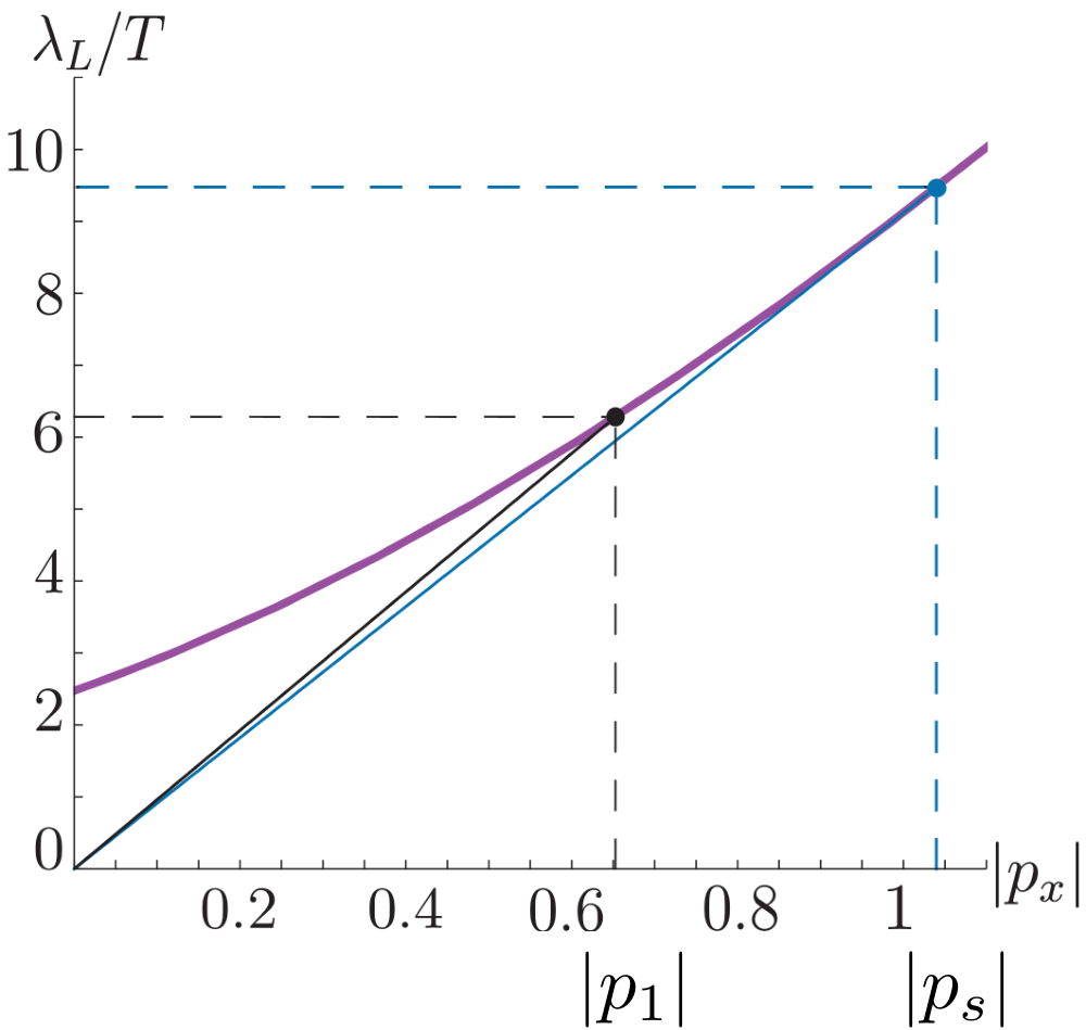
We note that does not depend upon the coupling , as can be removed by rescaling the external momentum . With no other dimensionful parameters in (9), this also implies that is proportional to temperature.
Phenomenological models. We extend our analysis to a general case of dynamic critical exponent , in which quasiparticle excitations are still absent, and compute the Lyapunov exponents. For those theories, the boson Green’s function has the form Esterlis et al. 2021
and the fermion self energy scales as ( for the original theory discussed earlier). Since , quasiparticle excitations are not well defined in terms of the fermion spectral function.
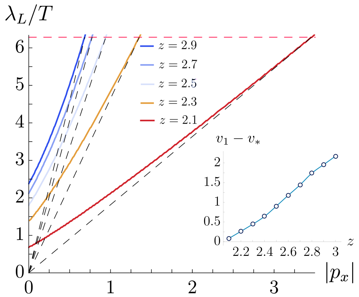
The form of the eigenvalue equation for the OTOC changes slightly, and is discussed in the Supplementary Information. As we show in the Fig. 5, for each of these theories the butterfly velocity is also given by , and the Lyapunov exponent is maximal. To show this, we first solve the eigenvalue equations up to the pole momentum . We then compare the instantaneous slope at , which we call , and the velocity . For each plot we obtain . Since each of the curves in Fig. 5 is a positive, monotonically increasing, and convex function, this implies that , and the pole contribution therefore dominates with maximal chaos just like in the case.
We can further find the behavior of the exponent in the case when , in which quasiparticles are present. In this regime, , and therefore the quasiparticle peak in the fermion spectral function is well defined. Similar to the discussion above, we can compute the Lyapunov exponent as a function of external momentum on imaginary axis and explicitly find and . For a particular case of 22 2 The numerical values of and are provided for chosen parameters , , , and . See Supplementary Information for more details., we find that the saddle point dominates as , which is smaller than . The resulting butterfly velocity in this case is , where is the Fermi velocity. This result is expected from a general point of view: for a free fermion theory the exponent is a simply linear function of the external momentum leading to the saddle point contribution at . We therefore expect that for any theory with quasiparticles, the pole contribution is negligible compared to a saddle point contribution, and the maximal chaos is therefore no longer present.
Discussion. It is quite remarkable that the generic low energy theory of Fermi surfaces without quasiparticles in dimensions display maximal chaos in the large limit. Other spatially extended quantum many body models connected to the SYK model (e.g. Gu et al. 2017; Kim et al. 2021), and certain conformal field theories Turiaci and Verlinde 2016; Haehl and Rozali 2018; Haehl et al. 2019, have been shown to display maximal chaos, but none of them have spatially dependent Green’s functions and live in more than one space dimension. Besides displaying maximal chaos in dimensions without exhibiting local criticality, it is also remarkable that the critical Fermi surface does so without the presence of conformal symmetry, which also sets it apart from the previously mentioned examples that have conformal symmetry.
We believe that the maximal chaos of the Fermi surface is linked to the local nature of the singular self energy of the fermion at large i.e. the self energy is frequency dependent, but independent of momentum, a feature the Fermi surface theory shares with the SYK model (along with the local frequency-only dependence of the fermion pairing vertex Esterlis et al. 2021). There are small contributions to the fermion anomalous dimension at 3-loop order Metlitski and Sachdev 2010, which are expected to make the self energy non-local, and it remains to be seen if such effects could reduce the maximal Lyapunov exponent. However, since is at large (Fig. 4), we expect that the small corrections to this quantity will not immediately be able to change its sign and thus reduce the maximal Lyapunov exponent.
We also examined a phenomenological model of a critical Fermi surface with dynamic critical exponent ; quasiparticles re-emerge in such a model for . We found that the maximal chaos was retained for precisely the regime where quasiparticles are absent, , although the size of the spactime region for which it occurs shrinks to zero as (Fig. 6). It is also remarkable that the acceleration of chaos to the maximal rate by the butterfly effect is tied to the destruction of quasiparticles in this model. When quasiparticles are present, we found that the saddle-point contribution dominated with , which is parametrically smaller than the maximal rate (Supplementary Information).
Acknolwedgements. We thank Haoyu Guo and Yingfei Gu for valuable discussions. M.T. and S.S. were supported by the National Science Foundation under Grant No. DMR-2002850. A.A.P. was supported by the Miller Institute for Basic Research in Science. This work was also supported by the Simons Collaboration on Ultra-Quantum Matter, which is a grant from the Simons Foundation (651440, S.S.).
References
- Hartnoll and Mackenzie (2021) S. A. Hartnoll and A. P. Mackenzie, Planckian Dissipation in Metals, (2021), arXiv:2107.07802 [cond-mat.str-el] .
- Chowdhury et al. (2021) D. Chowdhury, A. Georges, O. Parcollet, and S. Sachdev, Sachdev-Ye-Kitaev Models and Beyond: A Window into Non-Fermi Liquids, (2021), arXiv:2109.05037 [cond-mat.str-el] .
- Sachdev (1999) S. Sachdev, Quantum Phase Transitions (Cambridge University Press, Cambridge, UK, 1999).
- Bruin et al. (2013) J. A. N. Bruin, H. Sakai, R. S. Perry, and A. P. Mackenzie, Similarity of Scattering Rates in Metals Showing -Linear Resistivity, Science 339, 804 (2013).
- Zaanen (2004) J. Zaanen, Why the temperature is high, Nature 430, 512 (2004).
- Grissonnanche et al. (2021) G. Grissonnanche, Y. Fang, A. Legros, S. Verret, F. Laliberté, C. Collignon, J. Zhou, D. Graf, P. A. Goddard, L. Taillefer, and B. J. Ramshaw, Linear-in temperature resistivity from an isotropic Planckian scattering rate, Nature 595, 667 (2021), arXiv:2011.13054 [cond-mat.str-el] .
- Maldacena et al. (2016) J. Maldacena, S. H. Shenker, and D. Stanford, A bound on chaos, JHEP 08, 106, arXiv:1503.01409 [hep-th] .
- Maldacena and Stanford (2016) J. Maldacena and D. Stanford, Remarks on the Sachdev-Ye-Kitaev model, Phys. Rev. D 94, 106002 (2016).
- Kitaev and Suh (2018) A. Kitaev and S. J. Suh, The soft mode in the Sachdev-Ye-Kitaev model and its gravity dual, JHEP 05, 183, arXiv:1711.08467 [hep-th] .
- Lee (2018) S.-S. Lee, Recent Developments in Non-Fermi Liquid Theory, Annual Review of Condensed Matter Physics 9, 227 (2018), arXiv:1703.08172 [cond-mat.str-el] .
- Patel and Sachdev (2017) A. A. Patel and S. Sachdev, Quantum chaos on a critical Fermi surface, Proc. Nat. Acad. Sci. 114, 1844 (2017), arXiv:1611.00003 [cond-mat.str-el] .
- Gu and Kitaev (2019) Y. Gu and A. Kitaev, On the relation between the magnitude and exponent of OTOCs, JHEP 02, 075, arXiv:1812.00120 [hep-th] .
- Esterlis et al. (2021) I. Esterlis, H. Guo, A. A. Patel, and S. Sachdev, Large theory of critical Fermi surfaces, Phys. Rev. B 103, 235129 (2021), arXiv:2103.08615 [cond-mat.str-el] .
- Aldape et al. (2020) E. E. Aldape, T. Cookmeyer, A. A. Patel, and E. Altman, Solvable theory of a strange metal at the breakdown of a heavy Fermi liquid, (2020), arXiv:2012.00763 [cond-mat.str-el] .
- Lee (2009) S.-S. Lee, Low energy effective theory of Fermi surface coupled with U(1) gauge field in 2+1 dimensions, Phys. Rev. B 80, 165102 (2009), arXiv:0905.4532 [cond-mat.str-el] .
- Metlitski and Sachdev (2010) M. A. Metlitski and S. Sachdev, Quantum phase transitions of metals in two spatial dimensions. I. Ising-nematic order, Phys. Rev. B 82, 075127 (2010), arXiv:1001.1153 [cond-mat.str-el] .
- (17) For the single patch theory, the values of are given by and .
- (18) The numerical values of and are provided for chosen parameters , , , and . See Supplementary Information for more details.
- Gu et al. (2017) Y. Gu, X.-L. Qi, and D. Stanford, Local criticality, diffusion and chaos in generalized sachdev-ye-kitaev models, Journal of High Energy Physics 2017, 125 (2017).
- Kim et al. (2021) J. Kim, E. Altman, and X. Cao, Dirac fast scramblers, Phys. Rev. B 103, L081113 (2021).
- Turiaci and Verlinde (2016) G. J. Turiaci and H. Verlinde, On CFT and quantum chaos, Journal of High Energy Physics 2016, 1 (2016).
- Haehl and Rozali (2018) F. M. Haehl and M. Rozali, Effective field theory for chaotic CFTs, Journal of High Energy Physics 2018, 1 (2018).
- Haehl et al. (2019) F. M. Haehl, W. Reeves, and M. Rozali, Reparametrization modes, shadow operators, and quantum chaos in higher-dimensional CFTs, Journal of High Energy Physics 2019, 1 (2019).
See pages 1 of supplementalSee pages 2 of supplementalSee pages 3 of supplementalSee pages 4 of supplementalSee pages 5 of supplementalSee pages 6 of supplementalSee pages 7 of supplementalSee pages 8 of supplementalSee pages 9 of supplemental