Retinal Vessel Segmentation with Pixel-wise Adaptive Filters
Abstract
††footnotetext: ∗ Equal contribution. † Corresponding author: zhyuey@ustc.edu.cnAccurate retinal vessel segmentation is challenging because of the complex texture of retinal vessels and low imaging contrast. Previous methods generally refine segmentation results by cascading multiple deep networks, which are time-consuming and inefficient. In this paper, we propose two novel methods to address these challenges. First, we devise a light-weight module, named multi-scale residual similarity gathering (MRSG), to generate pixel-wise adaptive filters (PA-Filters). Different from cascading multiple deep networks, only one PA-Filter layer can improve the segmentation results. Second, we introduce a response cue erasing (RCE) strategy to enhance the segmentation accuracy. Experimental results on the DRIVE, CHASE_DB1, and STARE datasets demonstrate that our proposed method outperforms state-of-the-art methods while maintaining a compact structure. Code is available at https://github.com/Limingxing00/Retinal-Vessel-Segmentation-ISBI2022.
Index Terms:
Image segmentation, Retinal vessel, Siamese network, Segmentation refinement2 Institute of Artificial Intelligence, Hefei Comprehensive National Science Center
1 Introduction
Semantic segmentation is a fundamental task of biomedical image analysis, which can assist doctors in diagnosis and help biologists analyze cell morphology. In recent years, convolutional neural networks (CNNs) have shown remarkable effect on biomedical image segmentation. Among them, U-Net [1] is the most widely used semantic segmentation network, which consists of an encoder to extract image features and a decoder to reconstruct the segmentation result. U-Net++ [2] redesigns skip connections in the decoder, which improves the feature fusion and representation.
For the retinal vessel segmentation, previous methods can be roughly divided into three categories. The first category designs the topology-aware loss function to help the network recognize the critical structures [3, 4]. The second category utilizes multiple deep networks as the refinement module to refine the segmentation results [5, 6, 7]. The third category enhances the capacity of the single network to obtain richer and more complex feature maps, such as those using the attention mechanism [8, 9]. The method proposed in this paper belongs to the second category. Although the second category has satisfactory results, the deep networks are time-consuming and inefficient.
To this end, we propose a method to utilize only one layer of pixel-wise adaptive filters (PA-Filters) to refine the segmentation results instead of using deep networks. In order to learn PA-Filters, we propose a light-weight module, named multi-scale residual similarity gathering (MRSG). For each position on the initial segmentation map, MRSG generates a unique PA-Filter. Namely, unlike the traditional convolutional layer, the designed PA-Filters do not share weights to capture the texture of local regions better. Meanwhile, we propose a response cue erasing (RCE) strategy for further boosting the segmentation accuracy, which is implemented by an auxiliary branch. The RCE is responsible for erasing the corresponding position of the most confident pixels on the input image, depending on the output of the main branch. We design a regularization loss to control the consistency of the dual branches, which makes the network more robust. Experiments on three representative retinal vessel segmentation datasets (i.e. DRIVE, CHASE_DB1 and STARE) validate that our efficient network achieves state-of-the-art performance.
2 Method
2.1 Overview
As shown in Figure 1, in the training stage, there are two branches in the network, the main branch and the auxiliary branch. The two branches are weight-sharing. The only difference is the input images of the auxiliary branch is processed via the RCE strategy. Take the main branch as an example, the input image, , passes through a U-Net backbone to obtain a coarse segmentation map (). Then MRSG extracts the coarse segmentation map and input image to generate PA-Filters of size , where is a hyper-parameter. Next, PA-Filters are applied to the corresponding local regions on the coarse segmentation map to obtain the final segmentation map . During the testing stage, we only infer the main branch.

2.2 U-Net Backbone
We adopt U-Net as the backbone network . Given and , we can obtain the coarse segmentation map (). denotes the RCE operation. The formulation of can be written as
| (1) |
where denotes parameters of U-Net. Here we set the channel number of the coarse segmentation map to 1 instead of one-hot encoding which is convenient for the following process.

2.3 Multi-scale Residual Similarity Gathering
Inspired by prior works [10, 11], we adopt the similarity volume for gathering the context information depending on the neighbour pixels. As shown in Figure 2, for , we calculate the similarity value by element multiplication between every pixel and its neighbouring of pixels by the formula as follow:
| (2) |
where denotes the coordinate of the region. Thus, for every pixel, we can obtain a local representation. Then we concatenate the local representation along the channel dimension to obtain the similarity volume . Furthermore, inspired by ACNet [12] which indicates the skeletons are more important than the corners in a normal kernel, we find the closer pixels around the center pixel is more vital. Therefore, we propose a multi-scale residual scheme which adds the residual information for to obtain the final similarity volume . We make use of the similarity volume with a smaller for the residual information and introduce a bottleneck-style operation (a convolutional layer, a BatchNorm layer and a ReLU layer) to sum up different volumes. Based on the residual summation between similarity volumes, can be constructed from in a multi-scale procedure. We show the whole procedure and take as example in Equation 3:
| (3) | ||||
After obtaining , we reshape into PA-Filters of size . Then PA-Filters are applied to the corresponding local regions on the coarse segmentation map to obtain the final segmentation map .
2.4 Response Cue Erasing
To further exploit the potential of the network, we add an auxiliary branch and apply an RCE strategy for the input image of the auxiliary branch. As shown in Figure 1, we adopt the RCE to generate erased regions and adopt the regularization loss to control the consistency of the dual branches. The RCE has two steps. First, select the spatial position set , , corresponding to the highest confidence pixels of the coarse segmentation map , where both the foreground and background are considered. Second, erase the spatial position set of the input image. Different from random erasing which cannot capture the structures, the RCE generates structure-dependent mask on the input image.
2.5 The Overall Loss Function
We choose the dice loss [13] which measures the difference between the label and the main branch output as the segmentation loss . Besides, we propose the regularization loss for the dual branches, which can constrain the consistency of the two outputs. The overall loss is computed as
3 Experiments and Analysis
3.1 Datasets
We evaluate the proposed method on three popular retinal vessel segmentation datasets, DRIVE, CHASE_DB1 and STARE. Specifically, DRIVE [14] consists of 40 retinal images of size from a diabetic retinopathy screening program. Following the official partition, the training set has 20 images and the test set has the other 20 images. CHASE_DB1 [15] contains 28 retinal images of size . STARE [16] contains 20 retinal images of size . We follow the setting of the method in [6], which divides the first 20/16 images as the training set, and the last 8/4 images as the test set for these two datasets respectively.
3.2 Implementation Details
In the experiments, we utilize Pytorch (version 1.1) to implement the proposed method. An NVIDIA GTX 1080Ti is used for training and testing. During the training stage, we only use the flipping data augmentation. We minimize our loss using Adam, whose learning rate is 0.005 and fixed on the all datasets. We adopt the unified patch training strategy and set the patch size as 0.3 times the input image size. Thus the sampled patch sizes for the DRIVE, CHASE_DB1 and STARE datasets are , and respectively. We set batchsize 4 and maximum iteration 6000 on the three datasets. To balance the performance and computational burden, we choose for the PA-Filters in our experiments. We choose the suitable hyper-parameters and according to different datasets.
3.3 Quantitative and Qualitative Evaluation.

| Method | Param.(MB) | DRIVE | CHASE_DB1 | STARE | ||||||
|---|---|---|---|---|---|---|---|---|---|---|
| F1 | AUC | ACC | F1 | AUC | ACC | F1 | AUC | ACC | ||
| MS-NFN [5] | - | - | 98.07 | 95.67 | - | 98.25 | 96.37 | - | - | - |
| U-Net++ [2] | 9.162 | 81.92 | 98.12 | 96.88 | 81.34 | 98.35 | 97.62 | 78.59 | 97.63 | 97.57 |
| AG-Net [8] | 9.330 | 80.79 | 98.40 | 96.87 | 81.54 | 98.72 | 97.64 | 80.28 | 98.00 | 97.54 |
| HR-Net [17] | 3.883 | 82.50 | 98.20 | 96.93 | 81.22 | 98.30 | 97.63 | 79.30 | 96.92 | 97.52 |
| CTF-Net [18] | - | 82.41 | 97.88 | 95.67 | - | - | - | - | - | - |
| UCU-Net [19] | - | - | 97.24 | 95.40 | - | 97.63 | 96.01 | - | - | - |
| IterNet [6] | 8.251 | 82.50 | 98.04 | 96.89 | 81.21 | 98.15 | 97.46 | 81.33 | 96.89 | 97.82 |
| SCS-Net [20] | 3.700 | - | 98.37 | 96.97 | - | 98.67 | 97.44 | - | 98.77 | 97.36 |
| Ours | 2.013 | 82.61 | 98.43 | 96.99 | 81.67 | 98.35 | 97.61 | 81.70 | 98.43 | 97.88 |
We take F1-score (F1), area under curve (AUC), accuracy (ACC) as the metrics, which are evaluated by the open source [8]. Table 1 summarizes the parameter (Param.) and metrics of each state-of-the-art (SOTA) method on the DRIVE, CHASE_DB1 and STARE datasets. We can observe the proposed method has the best F1-score, surpassing other SOTA methods on all three datasets. Although AG-Net has the best AUC on the CHASE_DB1 dataset, the parameter of the proposed method is smaller than AG-Net, which shows the compactness of the proposed method. We also show the segmentation results on three datasets in Figure 3. Compared with other SOTA methods, our segmentation results have more detailed textures and complete structures.

3.4 Ablation Study
To verify the contribution of each component in the proposed method, we conduct the ablation study. As shown in Table 2, we evaluate the effectiveness of the PA-Filters and the RCE strategy. When we choose PA-Filters of size , the parameter of the network only increases by 0.012 MB, but F1-score increases by 3.1%. For the PA-Filters, we evaluate the impact of different kernel sizes without the RCE strategy. As shown in Table 3, a larger D achieves better performance at the cost of the requirement of larger GPU memory. Although has better performance, it exceeds the memory with the fixed setting (Section 3.2) on CHASE_DB1. For the sake of uniformity, our experiments are based on .
| PA-Filters | RCE | Param.(MB) | F1 | AUC | ACC | Time(ms) |
|---|---|---|---|---|---|---|
| 2.001 | 78.60 | 96.83 | 97.50 | 5.1 | ||
| 2.001 | 79.46 | 97.31 | 97.67 | 5.1 | ||
| 2.013 | 81.13 | 97.81 | 97.76 | 9.7 | ||
| 2.013 | 81.70 | 98.43 | 97.88 | 9.7 | ||
| Kernel Size (D) | w/o PA-Filters | 3 | 5 | 7 | 9 |
|---|---|---|---|---|---|
| Param. | 2.001 | 2.011 | 2.013 | 2.024 | 2.060 |
| Memory (GB) | 1.48 | 3.08 | 5.48 | 7.80 | 9.28 |
| F1-score | 78.60 | 80.96 | 81.13 | 81.78 | 81.95 |
| AUC | 96.83 | 97.47 | 97.81 | 97.79 | 97.73 |
3.5 Interpretability of the Proposed Method
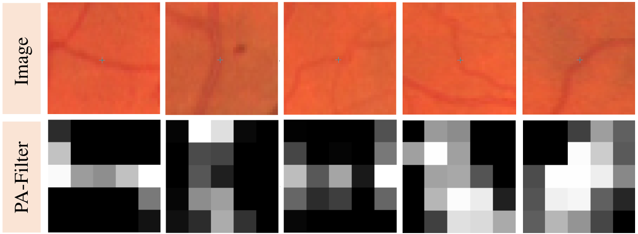
In the training stage, we have no supervision for the generation of the PA-Filters. As shown in Figure 4, PA-Filters learned at the central pixel implicitly reconstruct the texture of the retinal vessels instead of the local segmentation results. Taking the local patch of the first column of Figure 4 as an example, the PA-Filter learned from the center point is similar to the stripe. Note that the center point is on the border of retinal vessels. The learned PA-Filters implicitly learn the textures, which makes the coarse segmentation map pay attention to the vessel boundary. Therefore, as shown in Figure 5, the PA-Filter can refine the coarse segmentation results using only one layer.
4 Conclusion
In this paper, we propose PA-Filters and RCE strategy for retinal vessel segmentation. Specifically, we firstly utilize a U-Net backbone to obtain a coarse segmentation map, based on which the PA-Filters are generated. We devise an MRSG module to generate the PA-Filters for refinement. Moreover, an RCE strategy is proposed to further improve the performance. Experimental results on three representative retinal vessel datasets (DRIVE, CHASE_DB1 and STARE) demonstrate the superiority of the proposed method.
5 COMPLIANCE WITH ETHICAL STANDARDS
Ethical approval was not required as confirmed by the license attached with the open access data.
6 Acknowledgment
This work was supported in part by Anhui Provincial Natural Science Foundation Grant No. 1908085QF256 and University Synergy Innovation Program of Anhui Province No. GXXT-2019-025.
References
- [1] Olaf Ronneberger, Philipp Fischer, and Thomas Brox, “U-net: Convolutional networks for biomedical image segmentation,” in MICCAI, 2015.
- [2] Zongwei Zhou, Md Mahfuzur Rahman Siddiquee, Nima Tajbakhsh, and Jianming Liang, “Unet++: Redesigning skip connections to exploit multiscale features in image segmentation,” IEEE Transactions on Medical Imaging, vol. 39, no. 6, pp. 1856–1867, 2019.
- [3] Xiaoling Hu, Fuxin Li, Dimitris Samaras, and Chao Chen, “Topology-preserving deep image segmentation,” in NeurIPS, 2019.
- [4] Yuan Lan, Yang Xiang, and Luchan Zhang, “An elastic interaction-based loss function for medical image segmentation,” in MICCAI, 2020.
- [5] Yicheng Wu, Yong Xia, Yang Song, Yanning Zhang, and Weidong Cai, “Multiscale network followed network model for retinal vessel segmentation,” in MICCAI, 2018.
- [6] Liangzhi Li, Manisha Verma, Yuta Nakashima, Hajime Nagahara, and Ryo Kawasaki, “Iternet: Retinal image segmentation utilizing structural redundancy in vessel networks,” in WACV, 2020.
- [7] Mingxing Li, Yueyi Zhang, Zhiwei Xiong, and Dong Liu, “Cascaded attention guided network for retinal vessel segmentation,” in International Workshop on Ophthalmic Medical Image Analysis, 2020.
- [8] Shihao Zhang, Huazhu Fu, Yuguang Yan, Yubing Zhang, Qingyao Wu, Ming Yang, Mingkui Tan, and Yanwu Xu, “Attention guided network for retinal image segmentation,” in MICCAI, 2019.
- [9] Changlu Guo, Márton Szemenyei, Yugen Yi, Wenle Wang, Buer Chen, and Changqi Fan, “Sa-unet: Spatial attention u-net for retinal vessel segmentation,” arXiv preprint arXiv:2004.03696, 2020.
- [10] Deqing Sun, Xiaodong Yang, Ming-Yu Liu, and Jan Kautz, “Pwc-net: Cnns for optical flow using pyramid, warping, and cost volume,” in CVPR, 2018.
- [11] Tak-Wai Hui, Xiaoou Tang, and Chen Change Loy, “Liteflownet: A lightweight convolutional neural network for optical flow estimation,” in CVPR, 2018.
- [12] Xiaohan Ding, Yuchen Guo, Guiguang Ding, and Jungong Han, “Acnet: Strengthening the kernel skeletons for powerful cnn via asymmetric convolution blocks,” in ICCV, 2019.
- [13] Fausto Milletari, Nassir Navab, and Seyed-Ahmad Ahmadi, “V-net: Fully convolutional neural networks for volumetric medical image segmentation,” in 3DV, 2016.
- [14] Joes Staal, Michael D Abràmoff, Meindert Niemeijer, Max A Viergever, and Bram Van Ginneken, “Ridge-based vessel segmentation in color images of the retina,” IEEE Transactions on Medical Imaging, vol. 23, no. 4, pp. 501–509, 2004.
- [15] Christopher G Owen, Alicja R Rudnicka, Robert Mullen, Sarah A Barman, Dorothy Monekosso, Peter H Whincup, Jeffrey Ng, and Carl Paterson, “Measuring retinal vessel tortuosity in 10-year-old children: validation of the computer-assisted image analysis of the retina (caiar) program,” Investigative ophthalmology & visual science, vol. 50, no. 5, pp. 2004–2010, 2009.
- [16] AD Hoover, Valentina Kouznetsova, and Michael Goldbaum, “Locating blood vessels in retinal images by piecewise threshold probing of a matched filter response,” IEEE Transactions on Medical Imaging, vol. 19, no. 3, pp. 203–210, 2000.
- [17] Jingdong Wang, Ke Sun, Tianheng Cheng, Borui Jiang, Chaorui Deng, Yang Zhao, Dong Liu, Yadong Mu, Mingkui Tan, Xinggang Wang, et al., “Deep high-resolution representation learning for visual recognition,” IEEE Transactions on Pattern Analysis and Machine Intelligence, 2020.
- [18] Kun Wang, Xiaohong Zhang, Sheng Huang, Qiuli Wang, and Feiyu Chen, “Ctf-net: Retinal vessel segmentation via deep coarse-to-fine supervision network,” in ISBI, 2020.
- [19] Suraj Mishra, Danny Z Chen, and X Sharon Hu, “A data-aware deep supervised method for retinal vessel segmentation,” in ISBI, 2020.
- [20] Huisi Wu, Wei Wang, Jiafu Zhong, Baiying Lei, Zhenkun Wen, and Jing Qin, “Scs-net: A scale and context sensitive network for retinal vessel segmentation,” Medical Image Analysis, vol. 70, pp. 102025, 2021.