Deep inelastic collision of two-dimensional anisotropic dipolar condensate solitonsJournal: Commun. Nonlinear Sci. Numer. Simul.
Abstract
The possibility of generating stable anisotropic solitons in dipolar Bose-Einstein condensates (BECs) leads to a different scenario not possible in a nondipolar BEC with contact interaction. We study the statics and dynamics of anisotropic bright solitons in quasi-two-dimensional BECs consisting of polarized dipolar atoms. We study the collision dynamics of two such solitons at different velocities for different angles between the polarization and collision directions. The collision is found to be quasi elastic at large velocities. At small velocities the collision is inelastic leading to the formation of a coalesced soliton in an excited scissors mode, monopole mode or quadrupole mode. Also, at small velocities, after collision, a large change of direction of motion of the solitons is possible. The investigation is performed through a numerical solution of the underlying mean-field Gross-Pitaevskii equation.
1 Introduction
A bright soliton [1] is a self-bound localized object, that maintains its shape, while moving at a constant velocity in one-dimension (1D), due to a cancellation of dispersive effects and nonlinear attraction. The solitons can be both classical and quantum mechanical in nature. Quasi-one-dimensional (quasi-1D) solitons and soliton trains were created in a laboratory by considering strong traps in two transverse directions and studied experimentally in nondipolar quantum Bose-Einstein condensate (BEC) of 7Li [2] and 85Rb atoms [3] following a theoretical suggestion [4] in addition to 1D solitons in classical systems like water waves and nonlinear optics [1]. The quasi-1D geometry is created in a BEC by subjecting it to strong transverse traps along and directions and allowing the soliton to move freely along the direction. The BEC solitons constitute a fascinating consequence of a balance between the quantum-mechanical nonlinear attraction and the quantum-mechanical dispersive pressure thus resulting in self-confined wave-packets. The study of quasi-1D BEC solitons continues to be a very active field of research to date [5]. However, the nondipolar BEC solitons are fundamentally unstable in two [6] and three [1, 7] dimensions leading either to collapse or dispersion [8].
After the experimental observation of BECs of polarized 52Cr [9], 164Dy [10], and 168Er [11] atoms with large magnetic dipole moment, there has been a rapid growth of interest in dipolar BECs [12], which differ significantly from their non-dipolar counterparts due to the anisotropic long-range character of the dipole-dipole interaction. Polar molecules with large electric dipole moment were also considered for BEC experiments [13]. In addition to the usual quasi-1D nondipolar and dipolar BEC solitons, one can also have quasi-two-dimensional (quasi-2D) isotropic [14] as well as anisotropic [15] solitons in dipolar BECs polarized along the direction. A quasi-2D setting can be obtained in a laboratory by considering a strong trap in one direction. For a quasi-2D isotropic soliton the strong trap is in the polarization direction and for a quasi-2D anisotropic soliton the strong trap is in a direction perpendicular to the polarization direction. Moreover, solitons in a dipolar BEC remain stable when the transverse harmonic trap is replaced by a periodic optical-lattice trap in the quasi-2D [16] configuration. Both ground and exited states of quasi-2D solitons are found to be stable in polarized dipolar BECs under proper values of nonlinear dipolar and contact atomic interactions. More specifically, these quasi-2D dipolar solitons could be stable for a large repulsive nonlinear strength of contact repulsion with an even larger nonlinear strength of dipolar interaction [14, 15, 17], e.g., for a large atomic scattering length and for , where is a dipolar length, viz. Eq. (3), to measure the strength of dipolar interaction. Nevertheless, in general, an excited state can also be unstable. A large value of corresponding to a large short-range repulsion inhibits collapse to a great extent, whereas a large leads to a large long-range attraction to bind the soliton. Although, the dipolar interaction is repulsive in the direction perpendicular to polarization , a harmonic trap in the perpendicular direction suffices to form a quasi-2D robust anisotropic dipolar soliton free to move in the plane [15]. In spite of being one of the major novel features of the nonlinear physics of dipolar BEC, these quasi-2D solitons have not yet been observed in experiments, although quasi-2D Townes solitons [6] in a BEC were observed in two recent experiments [18]. In a different setting in nonlinear optics, however, a stable quasi-2D spatial soliton has been observed in liquid carbon disulfide [19].
Because of these interesting possibilities in dipolar BEC, we study here some novel features of the dynamics of anisotropic quasi-2D solitons [15] in a polarized dipolar BEC. Specifically, we investigate the collision dynamics of two robust quasi-2D dipolar solitons in the plane by varying the initial relative velocity and initial angle of impact using a mean-field Gross-Pitaevskii (GP) equation. In particular, we use two quasi-2D solitons with different angles between the collision directions of the two solitons in order to study a remarkable novel nonlinear feature of dipolar dynamics. At large velocities the dynamics is quasi-elastic for both head-on collision and collision with a non-zero impact parameter and the solitons pass through each other and move in straight line without significant deformation in shape. As the velocity is reduced the collision becomes inelastic and the emerging solitons become deformed. With further reduction in velocity the two solitons form a coalesced soliton in an excited state which eventually breaks up into few pieces that come out in directions independent of the initial directions of motion before collision. At very small initial velocities, the solitons come close to each other and form a coalesced single soliton and never separate. These latter inelastic processes through the formation of a coalesced soliton at small velocities will be called deep inelastic collision. These coalesced solitons are excited states of solitons where the initial kinetic energy is partially transformed into the internal excitation energy of the final soliton. In deep inelastic collision, after formation, the coalesced soliton often executes internal oscillations. The simplest mode of oscillation is monopole or breathing mode (radially symmetric contraction and expansion maintaining the shape.) The next excitation modes are dipole mode (contraction and expansion along one direction with change of shape) and quadrupole mode (simultaneous contraction and expansion along two directions with change of shape.) We find different types of excitation of the coalesced soliton. Specifically, we find a signature of scissors-mode and monopole mode oscillations [20] and dipole and quadrupole excitations in the coalesced soliton. Similar studies of collision of two quasi-1D dipolar solitons have identified the formation of a breathing mode [21]. The free angular oscillation of a BEC around an axis is called a scissors-mode oscillation. The scissors-mode oscillation in a BEC was detected [20] in the oscillation of a 87Rb BEC excited by a sudden rotation of the anisotropic trapping potential. In a nondipolar BEC, scissors-mode oscillation was initiated by external rotation [20]; here scissors-mode oscillation is initiated by inelastic collision between two dipolar solitons, while a part of the initial kinetic energy is transformed into angular oscillation energy. In case of scissors-mode oscillation the oscillation eventually die out and the solitons form a fused soliton in an excited state (soliton fusion). Also, at small initial velocities, a special coupling with internal soliton modes can appears and, interestingly enough, the direction of propagation of the solitons may change after collision. In numerical simulation we find a change of direction of propagation after collision. Many of the issues found in the numerical simulation of collision of two quasi-2D anisotropic dipolar solitons, including quasi-elastic reflection at large velocities and capture at small velocities, are encountered in other settings including collision between kink and antikink traveling waves of the equations of non-integrable field theories [22]. Formation of coalesced soliton molecules has also been studied experimentally in nonlinear fiber optics [23].
In Sec. 2.1 we describe the three-dimensional (3D) mean-field GP equation for a dipolar BEC. A reduced quasi-2D GP equation, which we employ for the present study of quasi-2D dipolar solitons, is given in Sec. 2.2. In Sec. 3 we describe the numerical results for a stationary quasi-2D soliton. Those for the dynamics of collision between two quasi-2D solitons at different velocities and for different angles of impact are presented in Sec. 4. Specifically, in Sec. 4.1 we consider quasi-elastic head-on collision at large velocities. In Sec. 4.2 quasi-elastic collision with a non-zero impact parameter is considered. In Sec. 4.3 results for deep inelastic collision at small velocities are presented; in Sec. 9 we consider a scissors-mode oscillation, in Sec. 4.3.2 an unexpected change in the direction of the emerging solitons, and finally in Sec.4.3.3 a quadrupole excitation of the coalesced soliton are considered. Finally, in Sec. 5 we provide a summary of our findings and conclusions.
2 Mean-field model for anisotropic dipolar BEC soliton
2.1 3D Gross-Pitaevskii equation
We consider a BEC of polarized dipolar atoms of mass each, interacting via the following atomic dipolar and contact interactions [12, 24]
| (1) |
where is the atomic scattering length, is the permanent magnetic dipole moment, is the permeability of vacuum, is the vector joining two dipoles placed at () and and is the angle made by with the polarization direction. At sufficiently low temperatures a dipolar BEC is described by the following nonlocal 3D GP equation [12, 24]
| (2) |
where is the external trap, the wave function is subject to normalization and .
In this study of quasi-2D solitons we consider a harmonic trap along the transverse direction, where is the trap frequency. To compare the dipolar and contact interactions, the strengths of the dipolar interaction is expressed in terms of the dipolar length
| (3) |
The dimensionless ratio characterizes the strength of dipole-dipole interaction compared to that of the short-range interaction .
2.2 Quasi-2D Reduction
In the presence of a harmonic potential along the -direction, it is natural to assume that the dynamics of the BEC in the direction is confined in the ground state of the harmonic potential and we have the following ansatz of the wave function
| (5) |
where , and is the asymmetric effective 2D wave function. To derive the effective 2D equation for the anisotropic quasi-2D dipolar BEC, we use ansatz (5) in Eq. (4), multiply it by the ground-state wave function and integrate over to get [15, 24, 25]:
| (6) |
The dipolar integral is calculated in momentum space by the following convolution rule [26]
| (7) |
where , the Fourier transformation of the 2D density [15, 27]
| (8) |
and
| (9) | |||||
where and is the complementary error function.
In two dimensions, in free space, a stable nondipolar BEC soliton cannot be formed due to a collapse instability [6]. For small values of nonlinear attraction such an object will escape to infinity and for large values of nonlinear attraction it will collapse. However, a weakly attractive BEC in a quasi-2D trap, below the Townes limit [6] of collapse, can be bound as the escape to infinity will not materialize due to the trap. It has been demonstrated [15] that, for moderate values of the scattering length and of the strength of dipolar interaction, the quasi-2D dipolar equation (6) without any external trap permits the formation of a spatially anisotropic soliton which can freely move in the plane. This soliton is supported only by a trap in the direction. Equation (6) is independent of the variable as the dependence on has been integrated out. Such a soliton will be extended in the plane and is, in general, called a quasi-2D soliton. Nevertheless, such a soliton collapses for large values of the strength of dipolar interaction (strong attraction for ) and escapes to infinity for large values of scattering length (strong repulsion for ), as we will see in the following. In this paper, the scattering length (and also ) is positive. A dipolar quasi-2D soliton with an appropriate value of can be prepared in a laboratory by manipulating the value of the scattering length by the Feshbach resonance technique [28]. The use of the quasi-2D GP equation (6) will facilitate the study of the formation of a strongly dipolar soliton and the collision dynamics of two such solitons. The quasi-2D dipolar soliton can be studied by a numerical solution of the full 3D GP equation (4). However, it is computationally more economic to solve the quasi-2D equation (6).
3 Result: Stationary soliton
We solve the full 3D GP equation (4) as well as the quasi-2D GP equation (6) numerically by the Crank-Nicolson discretization algorithm employing the split-time-step propagation method [29]. The dipolar interaction is treated by a convolution to the Fourier momentum space [26] using the available C and FORTRAN programs [24]. The stationary bound solitons were obtained by imaginary-time propagation whereas the real-time propagation was applied to study the dynamics of collision between two quasi-2D solitons. Nevertheless, the imaginary-time method has its limitations. This method may fail when the solution is unstable and the convergence is slow when the solution is close to unstable. There are the fixed-point schemes, like the variants of Newton-Raphson methods, and improved imaginary-time methods appropriate in these cases. Also, there are variants to imaginary-time methods, that are significantly better than the simple imaginary time methods [30]. These may not be of concern in the present study, as the solitons we will study are stable ground states and the dynamics of collision, often leading to unstable states, is studied by the real-time method.
In this paper we will present the results in dimensionless units and take the time scale to be 1 ms corresponding to the harmonic trap frequency Hz. The dimensionless results can be converted to actual physical results using the time scale (= 1 ms) and length scale . The values of the length scale , for this fixed time scale, are different for the commonly used dipolar atoms in BEC experiments, as the masses are different; for the dipolar atoms 52Cr, 164Dy, and 168Er the actual values of the length scale are m, 0.622 m, and 0.615 m, respectively. Hence the present dimensionless results can be transformed into actual physical units using these time and length scales for the common dipolar atoms used in BEC experiments.
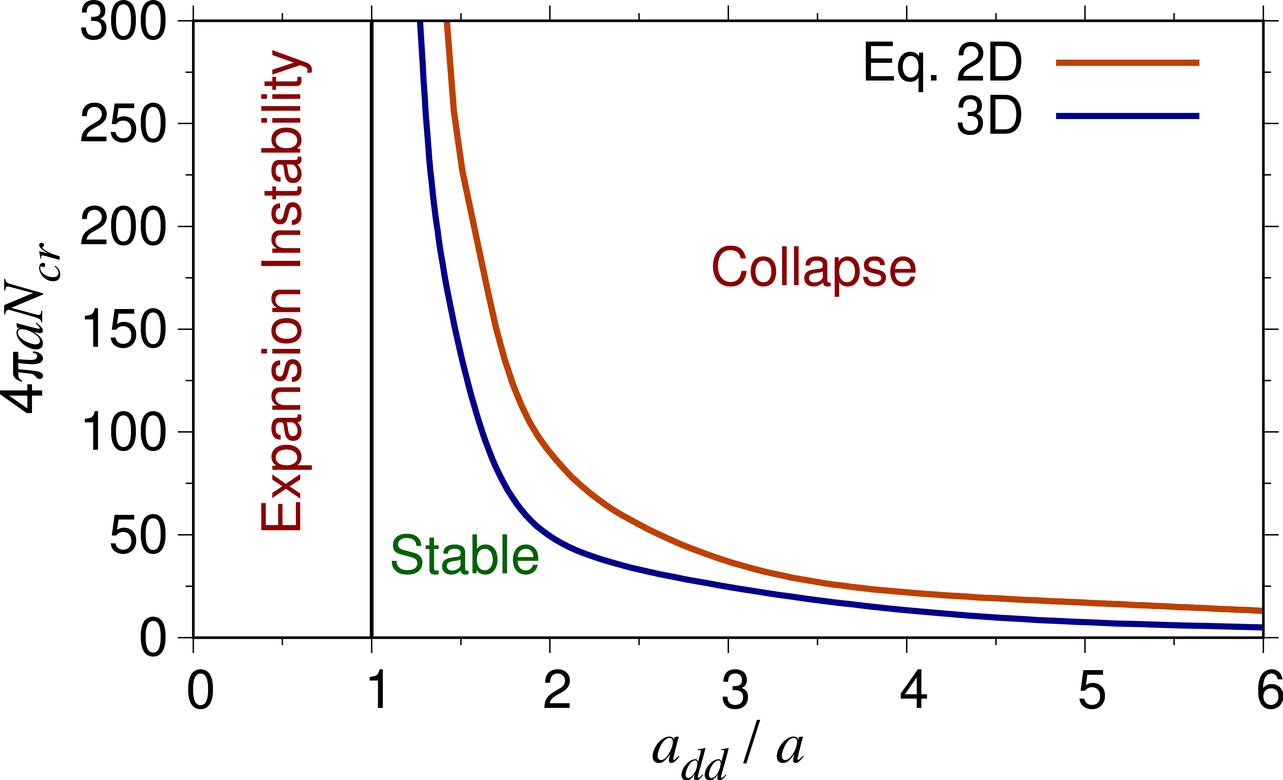
As it is commonly known, a BEC with dipolar interaction always becomes unstable and collapses when the number of particles is sufficiently large and greater than a critical number (), independent of the trapping geometry [31]. This is also true for the quasi-2D soliton described by Eq. (4) in 3D and Eq. (6) in 2D. A stability plot for the quasi-2D dipolar soliton is illustrated in Fig. 1 from numerical solutions of the 3D equation (4) and the quasi-2D equation (6) by imaginary-time propagation. The two results are in agreement with each other, specially for larger values of , where the soliton acquires a quasi-2D shape and validates the use of the quasi-2D equation (6). The stability phase diagram in Fig. 1 is consistent with previous results obtained by Santos et al. [17]. In the stable region, a balance between repulsive and attractive interactions allows the formation of stable solitons. However, in the expansion region, attractive dipolar interaction is not enough to compensate for the atomic contact repulsion; consequently, the soliton cannot be bound and will escape to infinity. In the collapse region the dipolar attraction is much larger than the contact repulsion and the soliton collapses.


In Fig. 2 we illustrate the shape of a stable anisotropic dipolar quasi-2D soliton showing the 3D contour plot of density obtained from a numerical solution of the 3D GP equation (4) by imaginary time propagation [29] for and . Because of the harmonic trap in the direction, the quasi-2D soliton is extended in the plane with a small width in the direction. The actual values of the ratio for the commonly used dipolar atoms is smaller than 3.35. For example, for 164Dy, [32], , for 168Er , , [33], for 52Cr [12] [34] [35], where is the Bohr radius. A smaller value of , and consequently, a larger , gives a quasi-2D shape of the soliton with small spatial extension along the perpendicular direction. In a laboratory a smaller value of can be achieved by the Feshbach resonance technique [28]. Such a modification of the atomic scattering length by a Feshbach resonance was necessary in all BEC experiments on solitons [2, 3, 5].
For an anisotropic quasi-2D soliton confined in the plane, it is appropriate to compare the reduced densities along and directions obtained from the 3D equation (4) and the quasi-2D equation (6) by integrating the respective densities over the orthogonal coordinates. The reduced densities are calculated from the 2D densities as
| (10) |
and from the 3D densities as
| (11) |
In Fig. 3 we compare these axial densities of the quasi-2D soliton of Fig. 2 obtained from the 3D and 2D equations. Based on the densities displayed in Fig. 3 and the stability plots of Fig. 1, we find that the 2D reduction Eq. (6) provides a faithful account of the actual state of affairs, when compared to the full 3D Eq. (4).
4 Result: Collision Dynamics
Starting with the initial anisotropic soliton wave function obtained by imaginary-time propagation we can obtain subsequent dynamics generated by real-time propagation of Eq. (6). The GP equation is Galilean invariant, hence a moving soliton, necessary for studying the collision dynamics, can be generated in a routine fashion in numerical simulation. A moving soliton traveling with a velocity can be trivially obtained in real-time simulation using a converged stationary solution of imaginary-time propagation multiplied by the phase factor as the initial function, provided an infinitely small space and time steps are used in numerical simulation.

Two such solitons, prepared by imaginary-time propagation, are placed in different spatial orientation at positions and time in the plane modifying the initial angle () between the collision direction and the axis of polarization . The respective imaginary-time wave functions are then multiplied by appropriate phase factors and then used as the initial states of real-time propagation so as to simulate the collision dynamics of two solitons at colliding frontally at the center with velocity .
A generic initial configuration of frontal collision of two dipolar solitons moving towards each other with velocity of components and is shown through contour density plots in Fig. 4. Three different initial configurations of the two colliding solitons for and are shown in Fig. 4 (a)-(c) through a contour plot of the respective densities. Of these, the orientation is interesting as strictly along this direction the interaction between two dimensionless point dipoles is zero [12]. The effective interaction between two solitons is the folding integral over the interatomic interactions between the atoms in the two solitons. Consequently, in the asymptotic region for angle °, when the two solitons are well separated, the effective dipolar interaction will be small, as the interatomic interactions around this angle will be small. For angle , the effective dipolar interaction between the two solitons will be repulsive as two point dipoles placed in side-by-side position repel [12]. For angle 90°, the effective dipolar interaction is attractive as two dipoles placed in head-to-tail position attract each other. Hence these three angles correspond to distinct dipolar asymptotic interactions between the solitons. For all these angles the isotropic nondipolar contact interaction in the asymptotic configuration is zero. In this way we study, in real-time simulation, the collision of two identical in-phase solitons placed as in Fig. 4. In quasi-elastic collision the emerging solitons are also in phase. We can use the variation in the initial conditions by varying the parameters and to explore the general dynamics involved in the collision process between two anisotropic dipolar quasi-2D solitons.

The complex dynamic processes involved in the collision between two anisotropic solitons in a dipolar BEC, which depend on the angle , is controlled by the velocity vector or by its two components and . The similar collision dynamics between two isotropic nondipolar collision is controlled only by the magnitude of the velocity vector and not by the components and , being independent of the colliding angle . To identify the domains of elastic and inelastic collisions, it is convenient to define the relative variation of soliton velocity vector and study its variation in the collision process for different angles . In Fig. 5 we elaborate a contour plot of the variation of the soliton velocity for collision of two identical solitons with and each as a function of the initial velocities and and of different angles . The angle in this plot is inherent in the sizes of and . For example, in this plot corresponds to and to °. Obviously, denotes fully inelastic collision with a total loss of the kinetic energy to inelastic excitation and denotes elastic collision with the conservation of kinetic energy. As expected, during soliton-soliton collision processes, the total energy of the system is conserved [36]. For large velocities in the region (E) of Fig. 5 the collision may be considered as quasi elastic and (black color in colorbar). However, for small velocities near the origin with (pink color in colorbar), the collision becomes inelastic. These different possibilities of inelastic excitation are further displayed in details in the inset of Fig. 5 for small .

Although at large velocities the collision between two solitons is quasi elastic with the conservation of total kinetic energy, as the velocity of the colliding solitons is reduced, the collision between two solitons gradually becomes inelastic with a deformation in the shape of two emerging solitons. In some of these inelastic collision processes at very small velocities we found evidence of coupling with special internal soliton modes, which will be called a deep inelastic process, such as scissors mode, quadrupole mode and even an interesting effect which produces an unexpected change in the direction of propagation of the emerging solitons. With a reduction in velocity, the incoming solitons may form a coalesced soliton in an excited state, which may break up into more than two pieces. In this region we identified an excitation to a dipole or quadrupole mode, viz. region (G) in Fig. 5. For even smaller velocities the excited coalesced soliton does not have enough energy to break up into multiple pieces, but eventually decays into two solitons that move apart in opposite directions distinct from the direction of motion of the incident soliton, viz. black line in the inset of Fig. 5. For sufficiently small velocities, the coalesced soliton does not have enough energy to break up and remain in an excited oscillating state, often undergoing oscillation in scissors mode or in monopolar breathing mode, viz. region (F) in Fig. 5. For the demarcation between regions (F) and (G), we performed simulation for collision for ten different angles between and 90°.
4.1 Head-on quasi-elastic collision
Only the collision between two integrable 1D solitons is truly elastic. However, for sufficiently large initial velocities, the collision between two quasi-2D dipolar solitons is found to be quasi-elastic with no visible change in shape and also in velocity after the collision, preserving the kinetic energy. In this case, the relative distance between the two centers of mass increases with time after the collision. We consider the head-on collision between two solitons, initially placed at at an angular orientation and attributed a velocity of so as to collide frontally. In Fig. 6) we illustrate the quasi-elastic nature of this collision using the contour plot of 2D density , through snapshots of density at different times before (, 26), during ( 50) and after ( 90, and 115) collision. The quasi-elastic nature of collision becomes more explicit from a plot of the reduced density during collision. The reduced densities , viz. Eq. (10), of the colliding solitons at different times before (, 34), during () and after (, 128) collision are displayed in Fig. 7. We find in Fig. 7 that the reduced densities at time and , before and after collision, respectively, are practically the same. The quasi-symmetric profile of during collision demonstrates that the solitons come out practically unchanged after collision and the quasi-elastic nature of collision is confirmed from a comparison of densities at and in Fig. 7. A video clip of the collision dynamics of Fig. 6 is prepared and contained in supplementary file head-on-quasi-elastic-collision.mp4 and also the video available at https://youtu.be/BnZLlVsIGe0 .

4.2 Quasi-elastic collision with an impact parameter
We also studied quasi-elastic collision with a non-zero impact parameter and moving along the direction. For this we considered two solitons placed at and at and attributed the velocity along the direction with °so as to collide at with an impact parameter of 10. In this case the soliton continues to move along the direction after collision without any deformation in shape or notable change of velocity or direction of motion along direction. Such a collision could introduce a rotation in the solitons after collision or a change in the direction of motion. No such rotation is found in this case or change in the direction of motion, viz. Fig. 8. We performed numerical simulation for different values of the impact parameter but the outcome remains unchanged. A video clip of the collision dynamics of Fig. 8 is contained in supplementary file quasi-elastic-with-impact-parameter10.mp4 and also video available at https://www.youtube.com/watch?v=5AKpui0tlYY .
4.3 Deep inelastic collision
As the velocity is reduced the collision becomes inelastic and the emerging solitons after collision are deformed in shape but maintain the initial directions of motion. Upon further reduction in velocity, the two colliding solitons form a coalesced soliton in a highly excited state performing oscillation, which eventually breaks up, often into more than two pieces. In this case the coalesced soliton does not “remember" the incident directions of motion and the emerging solitons come out in directions independent of the initial directions. The collision in this case (with velocities corresponding to the inset of Fig. 5) will be called deep inelastic collision. In the following we consider three distinct phenomena encountered in deep inelastic collision. The process of deep inelastic collision is quite similar to compound nuclear reaction [37]. In compound nuclear reaction, two low-energy colliding nuclei form a compound nucleus in an excited state, which do not remember the details of the incident nuclei and eventually breaks up into different pieces which come out in directions independent of those of the directions of motion of the incident nuclei.
4.3.1 Scissors-mode oscillation and soliton fusion


We next study the formation of a coalesced soliton executing scissors-mode oscillation, viz. region (F) in Fig. 5, in deep inelastic collision of two anisotropic quasi-2D dipolar solitons, each with and , placed at , with an initial angle between the collision direction and the axis of polarization and with an initial velocity of at . In this angular orientation the dipolar interaction between two point dipoles is zero and that between the two solitons is supposed to be small when separated by a distance large compared to their size. We plot in Fig. 9 the contour density at different times before (a) , during (b) , and after (c) , (d) , (e) , (f) , (g) , (h) , (i) and (j) 2640 collision. The formation of the coalesced soliton is complete in plot (c) at time . The initial orientation of the prolate solitons in (a) is along the axis. The slowly colliding solitons merge into a single coalesced soliton in (c), whose orientation is different from the original (vertical) one. We find in (b), (c) and subsequent plots two small separated pieces resembling the density of an angular momentum state usually called a dipole excitation, which eventually subsides.
In the deep inelastic collision of two anisotropic quasi-2D dipolar solitons we find the signature of scissors-mode oscillation. The orientation of the prolate soliton after formation in Fig. 9 also performs a few angular scissors-mode oscillations, and eventually forms a fused soliton, which relaxes along the polarization axis in (j) due to the dipolar interaction. During this process the kinetic energy of oscillation is changed to internal excitation energy of the fused soliton. We illustrate this scissors mode in the dynamic collision using the Figs. 9 (c)-(i) to show the oscillation of density cloud around the axis, and after some time, Fig. 9 (j), the system is fully oriented along the direction of polarization. In plots (c) to (e) the soliton turns to right, and then turns to left in plots (e) to (g), then to right in plots (g) to (i) and then to left to relax along the polarization direction in plot (j).

As a coalesced soliton aligns itself eventually along the polarization direction because of dipolar interaction, it is not possible to have the final coalesced soliton aligned in a direction different from the axis. After formation, the coalesced soliton shrinks in size and its central density attains a maximum and the soliton continues a monopole breathing oscillation (radial contraction and expansion) for a long time. To demonstrate this oscillation explicitly, we plot in Fig. 10 the maximum value of density after collision versus time. We have continued the plot in Fig. 10 for times well beyond that shown in Fig. 9. The maximum value of density is small in the beginning and attains a maximum value during collision between time and , i.e., after the formation of the coalesced soliton. Then for the maximum density keeps on oscillating as the coalesced soliton executes a breathing oscillation during a very long period of time with a period of approximately 1000 time units and with a decaying amplitude. The continued oscillation of density demonstrates the robustness of this new coalesced state for large time. A video clip of the fusion dynamics of Figs. 9 and 10, to show the breathing-mode and scissors-mode oscillations, is also prepared and contained in supplementary file scissors-mode.mp4 and also available at https://youtu.be/LB8b8JKOmKA .
4.3.2 Change in direction of propagation

Interestingly, some of the deep inelastic collision processes show an unexpected change in the direction of propagation for both solitons after the collision: viz. the full black line in the inset of Fig.5. This is a classic example of deep inelastic collision, where the final emerging solitons come out in directions completely independent of the directions of the incoming solitons. We illustrate in Fig. 11, a collision process for two anisotropic quasi-2D solitons initially placed at , with initial velocity of about and an initial angle of between the collision direction and the axis at . The contour of density at different times before (1-3), during (4 and 5) and after (6-9) collision in Fig. 11 is showing that the direction of propagation suddenly changes. This happens due to the formation of a coalesced soliton in an highly excited state. Due to an excessive energy, this soliton eventually decays into two solitons which move apart in opposite directions, distinct from the incident direction. The arrows in Fig. 11 represent the direction of propagation for both solitons before and after collision showing a drastic change in the propagation direction of the solitons. After the collision, the angle between the collision direction and the axis of polarization changes to the final value from the initial value before collision. A video clip of the inelastic collision process of Fig. 11 is available in supplementary file change-direction-propagation.mp4 and also available at https://youtu.be/IIH1y7zrfpk .

4.3.3 Excitation to a quadrupole mode
We show in Fig. 12 the evidence of coupling to a quadrupole mode, through a plot of the contour of density of two anisotropic solitons with each in a collision with initial velocity and for different times before (a) , during (b) and after (c) , (d) and (e) collision. This velocity corresponds to region (G) of Fig. 5. Independently of the value of , the solitons form a highly excited coalesced soliton after collision, which eventually decays into four pieces. The formation of the coalesced soliton is complete in (c). In plots (b) and (c) the density distribution is similar to dipole excitation, then it enters a configuration in (d) resembling a quadrupole excitation, then expands further in (e) maintaining the quadrupole shape. It continues this expansion and breaks up into four pieces, which move apart and never come back due to an excess of energy of the coalesced soliton. This process is found in all initial angles for . A video clip of this deep inelastic dynamics of Fig. 12 is contained in supplementary file quadrupole-mode.mp4 and also available at https://youtu.be/EoaWDzmU-qE .
5 Summary
To summarize, using a numerical solution of the mean-field 3D and quasi-2D GP equations, we studied the formation of anisotropic quasi-2D dipolar BEC solitons [15], mobile in the plane, polarized along the axial direction and harmonically trapped along the transverse direction. In this paper we considered frontal collision as well as collision with a non-zero impact parameter between two anisotropic dipolar soliton at different velocities and for different angles between the direction of motion and the polarization direction. At large velocities of collision, the collision is found to be quasi elastic with no visible deformation of soliton profiles after collision. As the velocity is reduced, the collision becomes inelastic with deformation of soliton profiles after collision and the deformation increases at slower velocities. For even slower velocities the solitons form an unstable coalesced soliton in a highly excited state which decays eventually into more than two pieces. In this region we identified a quadrupole excitation of the coalesced soliton and a subsequent decay to four solitons. For further reduction of velocity, the coalesced soliton decays into two solitons moving away in direction different from the incident direction. At sufficiently small velocities the fused coalesced soliton does not have sufficient energy for break up and performs oscillation in complex modes (soliton fusion); the signature of scissors mode (angular oscillation) and breathing mode (radial expansion and contraction) are found in numerical simulation. The result of collision for frontal collision and collision with a non-zero impact parameter are quite similar for both quasi-elastic, viz. Sec. 4.2, and inelastic collision (not reported here). It has been demonstrated numerically that these robust anisotropic quasi-2D dipolar solitons can be created in a laboratory from trapped dipolar BECs by suitably changing the trap frequency and the scattering length thus making the collision of such solitons possible in a laboratory [38].
Credit author statement
Both authors were responsible for Conceptualization, Methodology, and Software. L. E. Young-S. was responsible for Formal Analysis, Investigation, Data Curation and Writing - Original Draft. S. K. Adhikari was responsible for Writing - Review and Editing and Supervision.
Acknowledgments
We thank Prof. L. Santos for his kind interest in this study and many valuable suggestions. S.K.A. acknowledges support by the CNPq (Brazil) grant 301324/2019-0, and by the ICTP-SAIFR-FAPESP (Brazil) grant 2016/01343-7.
References
- [1] Y. S. Kivshar, B. A. Malomed, Rev. Mod. Phys. 61 (1989) 763; F. K. Abdullaev, A. Gammal, A. M. Kamchatnov, L. Tomio, Int. J. Mod. Phys. B 19 (2005) 3415.
- [2] K. E. Strecker, G. B. Partridge, A. G. Truscott, R. G. Hulet, Nature 417 (2002) 150; L. Khaykovich, F. Schreck, G. Ferrari, T. Bourdel, J. Cubizolles, L. D. Carr, Y. Castin, C. Salomon, Science 256 (2002) 1290.
- [3] S. L. Cornish, S. T. Thompson, C. E. Wieman, Phys. Rev. Lett. 96 (2006) 170401.
- [4] V. M Pérez-García, H. Michinel, H. Herrero, Phys. Rev. A 57 (1998) 3837.
- [5] D. Luo, Y. Jin, J. H. V. Nguyen, B. A Malomed, O. V. Marchukov, V. A Yurovsky, V. Dunjko, M. Olshanii, R. G. Hulet, Phys. Rev. Lett. 125 (2020) 183902; O. V. Marchukov, B. A. Malomed, V. A. Yurovsky, M. Olshanii, V. Dunjko, R. G. Hulet, Phys. Rev. A 99 (2019) 063623; V. A Yurovsky, B. A. Malomed, R. G. Hulet, M. Olshanii, Phys. Rev. Lett. 119 (2017) 220401; J. H. V. Nguyen, D. Luo, R. G. Hulet, Science 356 (2017) 422.
- [6] R. Y. Chiao, E. Garmire, C. H. Townes, Phys. Rev. Lett. 13, 479 (1964).
- [7] S. K. Adhikari, Phys. Rev. A 69, 063613 (2004).
- [8] E. A. Donley, N. R. Claussen, S. L. Cornish, J. L. Roberts, E. A. Cornell, C. E. Wieman, Nature 412, 295 (2001).
- [9] T. Lahaye, T. Koch, B. Fröhlich, M. Fattori, J. Metz, A. Griesmaier, S. Giovanazzi, T. Pfau, Nature 448 (2007) 672; A. Griesmaier, J. Stuhler, T. Koch, M. Fattori, T. Pfau, S. Giovanazzi, Phys. Rev. Lett. 97 (2006) 250402.
- [10] M. Lu, N. Q. Burdick, S. H. Youn, B. L. Lev, Phys. Rev. Lett. 107 (2011) 190401.
- [11] K. Aikawa, A. Frisch, M. Mark, S. Baier, A. Rietzler, R. Grimm, F. Ferlaino, Phys. Rev. Lett. 108 (2012) 210401.
- [12] T Lahaye, C Menotti, L Santos, M Lewenstein, T Pfau, Rep. Prog. Phys. 72 (2009) 126401.
- [13] J. Deiglmayr, A. Grochola, M. Repp, K. Mörtlbauer, C. Glück, J. Lange, O. Dulieu, R. Wester, M. Weidemüller, Phys. Rev. Lett. 101 (2008) 133004; M. H. G. de Miranda, A. Chotia, B. Neyenhuis, D. Wang, G. Quéméner, S. Ospelkaus, J. L. Bohn, J. Ye, D. S. Jin, Nature Phys. 7 (2011) 502.
- [14] P. Pedri, L. Santos, Phys. Rev. Lett. 95 (2005) 200404.
- [15] I. Tikhonenkov, B. A. Malomed, A. Vardi, Phys. Rev. Lett. 100 (2008) 090406.
- [16] S. K. Adhikari, P. Muruganandam, J. Phys. B. 45 (2012) 045301.
- [17] R. Nath, P. Pedri, L. Santos, Phys. Rev. Lett. 102 (2009) 050401.
- [18] C.-A. Chen and C.-L. Hung, Phys. Rev. Lett. 125 (2020) 250401; B. Bakkali-Hassani, C. Maury, Y.-Q. Zou, É. Le Cerf, R. Saint-Jalm, P. C. M. Castilho, S. Nascimbene, J. Dalibard, J. Beugnon, arXiv:2103.01605.
- [19] E. L. Falcão-Filho, C. B. de Araújo, G. Boudebs, H. Leblond, V. Skarka, Phys. Rev. Lett. 110 (2013) 013901.
- [20] O.M. Maragò, S.A. Hopkins, J. Arlt, E. Hodby, G. Hechenblaikner, C.J. Foot, Phys. Rev. Lett. 84 (2000) 2056.
- [21] P. Gao, X. Li, Z.-Y. Yang, W.-L. Yang, S. Yi, J. Phys. B 54 (2021) 135301.
- [22] R. H. Goodman, R. Haberman, SIAM J. Appl. Dyn. Syst 4 (2005) 1195.
- [23] M. Stratmann, T. Pagel, F. Mitschke, Phys. Rev. Lett. 95 (2005) 143902.
- [24] R. Kishor Kumar, Luis E. Young-S., D. Vudragović, A. Balaž, P. Muruganandam, S. K. Adhikari, Comput. Phys. Commun. 195 (2015) 117.
- [25] L Salasnich, A Parola, L Reatto, Phys. Rev. A 65 (2002) 043614.
- [26] K. Góral, L. Santos, Phys. Rev. A 66 (2002) 023613.
- [27] C. Ticknor, R. M. Wilson, J. L. Bohn, Phys. Rev. Lett. 106 (2011) 065301.
- [28] S. Inouye, M. R. Andrews, J. Stenger, H.-J. Miesner, D. M. Stamper-Kurn, W. Ketterle, Nature 392 (1998) 151.
- [29] P. Muruganandam, S. K. Adhikari, Comput. Phys. Commun. 180 (2009) 1888;
- [30] J. Yang and T. I. Lakoba, “Accelerated Imaginary-time Evolution Methods for the Computation of Solitary Waves”, Stud. Appl. Math. 120, 265 (2008).
- [31] T. Koch, T. Lahaye, J. Metz, B. Fröhlich, A. Griesmaier, T. Pfau, Nature Phys. 4 (2008) 218.
- [32] Y. Tang, A. Sykes, N. Q. Burdick, J. L. Bohn, B. L. Lev, Phys. Rev. A 92 (2015) 022703.
- [33] K. Aikawa, A. Frisch, M. Mark, S. Baier, R. Grimm, F. Ferlaino, Phys. Rev. Lett. 112 (2003) 010404; PhD thesis of Baier Simon, submitted to the Faculty of Mathematics, Computer Science, and Physics of the University of Innsbruck, available at http://www.erbium.at/FF/wp-content/uploads/2018/10/Dissertation_Simon_Baier.pdf
- [34] P. O. Schmidt, S. Hensler, J. Werner, A. Griesmaier, A. Görlitz, T. Pfau, A. Simoni, Phys. Rev. Lett. 91 (2003) 193201.
- [35] A. Griesmaier, J. Stuhler, T. Koch, M. Fattori, T. Pfau, S. Giovanazzi. Phys. Rev. Lett. 97 (2006) 250402; G. Herink, F. Kurtz, B. Jalali, D. R. Solli, C. Ropers, Science 356 (2017) 50.
- [36] R. Nath, P. Pedri, L. Santos, Phys. Rev. A 76 (2007) 013606.
- [37] P. Fröbrich, R. Lipperheide, Theory of Nuclear Reactions, 1st Eds., Clarendon Press, Oxford (1996).
- [38] P. Köberle, D. Zajec, G. Wunner, B. A. Malomed, Phys. Rev. A 85 (2012) 023630.