Scattering in terms of Bohmian conditional wave functions for scenarios with non-commuting energy and momentum operators

The full quantum Hamiltonian $\hat{H}=\hat{H}_{e}+\hat{H}_{\gamma}+\hat{H}_{I}$ that describes light-matter interaction is given by the sum of the electron Hamiltonian $\hat{H}_{e}$, the electromagnetic field Hamiltonian $\hat{H}_{\gamma}$, and the electron-photon interaction Hamiltonian $\hat{H}_{I}$. In particular, for a single electron in a semiconductor, the position representation for $\hat{H}_{e}$ (assuming a 1D system for the electron with degree of freedom $x$) is given by

$$H_{e}=-\frac{\hbar^{2}}{2m^{*}}\frac{\partial^{2}}{\partial x^{2}}+V(x),$$

(8)

where $V(x)$ includes both internal and external electrostatic potential. See the blue electron wave packet and the scalar potential $V(x)$ for a double barrier region of length $2L_{x}$ in the horizontal $x$-axis of Fig. 1(a).

We consider that the electromagnetic field is described by a single mode with angular frequency $\omega$ inside a closed cavity of length $2L_{M}$. See the cyan mirrors in the horizontal $x$-axis of Fig. 1(a) and (b). The typical description of the electric field will be $E(x,t)\propto q\;cos(kx-\omega t)$ with the wave vector $k=2\pi/\lambda$ related to the angular frequency as $c=\omega/k$ with $c$ the speed of light. The variable $q$ represents the instantaneous amplitude of the electromagnetic field along the polarization vector. Under the assumption $L_{M}\gg L_{x}$ meaning that the wave-length for the electromagnetic wave ($\approx 500$ nm) is much larger than the active region ($\approx 20$ nm), we can neglect the spatial dependence $x$ of the electromagnetic field. Then, the Hamiltonian of the electromagnetic field in second quantization can be written as $\hat{H}_{\gamma}=\hbar\omega\left(1/2+\hat{a}^{\dagger}\hat{a}\right)$. The relationship between the now quantized amplitude of the electric field $q$ and the creation $\hat{a}^{\dagger}$ and annihilation operators $\hat{a}$ is given by

$$\hat{a}=\sqrt{\frac{\omega}{2\hbar}}\left(q+\frac{\hbar}{\omega}\frac{\partial}{\partial q}\right)\;\;\;\;,\;\;\;\hat{a}^{\dagger}=\sqrt{\frac{\omega}{2\hbar}}\left(q-\frac{\hbar}{\omega}\frac{\partial}{\partial q}\right).$$

(9)

Then, the q-representation of $\hat{H}_{\gamma}$ is

$\displaystyle H_{\gamma}=-\frac{\hbar^{2}}{2}\frac{\partial^{2}}{\partial q^{2}}+\frac{\omega^{2}}{2}q^{2},$

(10)

where the electromagnetic vacuum state with zero photons $|0\rangle$ solution of $\hat{H}_{\gamma}$ corresponds to the ground state of a harmonic oscillator $\psi_{0}(q)=\langle q|0\rangle$, while the state solution of $\hat{H}_{\gamma}$ with one photon corresponds to the first excited state of an harmonic oscillator $\psi_{1}(q)=\langle q|\hat{a}^{\dagger}|0\rangle$.

The interaction Hamiltonian in the dipole approximation can be written as $\hat{H}_{I}=-e\hat{x}\hat{E}$, where $e$ is the (unsigned) electron charge and the electrical field operator is given by $\hat{E}=\epsilon\left(\hat{a}+\hat{a}^{\dagger}\right)$, with $\epsilon$ the strength of the electric field, or explicitly as

$\displaystyle H_{I}=\alpha^{\prime}xq$

(11)

where $\alpha^{\prime}$, which depends on $\epsilon$ and other parameters of the cavity, controls the strength of the light-matter interaction. Finally, the wave function $\Psi(x,q,t)$ that describes the quantum nature of electrons and the electromagnetic field simultaneously in the $q$-representation is solution of the following two-dimensional Schrödinger equation,

	$\displaystyle i\hbar\frac{\partial\Psi(x,q,t)}{\partial t}=$	$\displaystyle-$	$\displaystyle\frac{\hbar^{2}}{2m}\frac{\partial^{2}\Psi(x,q,t)}{\partial x^{2}}+V(x)\Psi(x,q,t)$		(12)
		$\displaystyle-$	$\displaystyle\frac{\hbar^{2}}{2}\frac{\partial^{2}\Psi(x,q,t)}{\partial q^{2}}+\frac{\omega^{2}}{2}q^{2}\Psi(x,q,t)$
		$\displaystyle+$	$\displaystyle\alpha^{\prime}xq\Psi(x,q,t).$

To simplify our discussion of emission and absorption of a photon by an electron, let us assume that only the zero photon state, $\psi_{0}(q)=\langle q|0\rangle=\langle q|\psi_{0}\rangle$, and the one photon state, $\psi_{1}(q)=\langle q|\hat{a}^{\dagger}|0\rangle=\langle q|\psi_{1}\rangle$, are relevant in our active region. Notice that we are discussing the interaction of a single electron with a single photon. Then, we can rewrite the wave function $\Psi(x,q,t)$ solution of (12) as

$\displaystyle\Psi(x,q,t)=\psi_{A}(x,t)\psi_{0}(q)+\psi_{B}(x,t)\psi_{1}(q),$

(13)

with

	$\displaystyle\psi_{A}(x,t)=\int\;\psi_{0}^{*}(q)\Psi(x,q,t)dq$		(14)
	$\displaystyle\psi_{B}(x,t)=\int\;\psi_{1}^{*}(q)\Psi(x,q,t)dq.$		(15)

The equation of motion of $\psi_{A}(x,t)$ and $\psi_{B}(x,t)$ can be obtained by introducing the definition (13) into (12) and using the orthogonality of $\psi_{0}(q)$ and $\psi_{1}(q)$ as follows

	$\displaystyle i\hbar\frac{\partial\psi_{A}(x,t)}{\partial t}=$	$\displaystyle-$	$\displaystyle\frac{\hbar^{2}}{2m}\frac{\partial^{2}\psi_{A}(x,t)}{\partial x^{2}}$		(16)
		$\displaystyle+$	$\displaystyle\left(V(x)+\frac{1}{2}\hbar\omega\right)\psi_{A}(x,t)$
		$\displaystyle+$	$\displaystyle\alpha x\psi_{B}(x,t),$
	$\displaystyle i\hbar\frac{\partial\psi_{B}(x,t)}{\partial t}=$	$\displaystyle-$	$\displaystyle\frac{\hbar^{2}}{2m}\frac{\partial^{2}\psi_{B}(x,t)}{\partial x^{2}}$		(18)
		$\displaystyle+$	$\displaystyle\left(V(x)+\frac{3}{2}\hbar\omega\right)\psi_{B}(x,t)$
		$\displaystyle+$	$\displaystyle\alpha x\psi_{A}(x,t),$

where we have defined $\alpha=\alpha^{\prime}\int\psi_{0}(q)q\psi_{1}(q)dq$ and we have used $\int\psi_{0}(q)q\psi_{0}(q)\;dq=\int\psi_{1}(q)q\psi_{1}(q)\;dq=0$.

We simulate now an initial electron impinging on a double barrier with a potential energy $V(x)$ as shown in Fig. 2 (a). It corresponds to the conduction band of a typical resonant tunnelling diode (RTD) with a 10 nm-well width, barrier thickness of 2 nm, and barrier height of 0.5 eV. In Fig. 2 (b), the transmission coefficient of the double barrier is plotted showing two resonant energies inside the well at $E_{1}=0.058$ eV and $E_{2}=0.23$ eV. The positive energies correspond to energy eigenstates impinging from the left and negative energies from the right.

At the initial time, we assume that there are no photons inside the active region. In other words, the (vacuum) electromagnetic field is given by an amplitude $q$ with probability $|\psi_{0}(q)|^{2}$. Thus, we define $\psi_{A}(x,0)$ as a Gaussian wave packet outside of the barrier region with a central energy equal to the second resonant level of the double barrier $E_{2}$ and a spatial dispersion of $30$ nm, as seen in the blue wave packet in the $x$-axis of Fig. 1(a), and $\psi_{B}(x,0)=0$. Thus, the initial electron-photon wave function in expression (13) is given only by $\Psi(x,q,t)=\psi_{A}(x,t)\psi_{0}(q)$. When solving (16) and (18), together, with $\alpha=2.5\cdot 10^{7}eV/m$ and $\omega=(E_{2}-E_{1})/\hbar$ we obtain that $\psi_{B}(x,t)\neq 0$ so that the global wave function in (13) becomes $\Psi(x,q,t)=\psi_{A}(x,t)\psi_{0}(q)+\psi_{B}(x,t)\psi_{1}(q)$. This process of spontaneous emission cannot be understood without the quantization of the electromagnetic field done in (12).

Next, to compute how much probability inside the well can be assigned to $\psi_{A}(x,t)$ and $\psi_{B}(x,t)$, at each resonant level, we define

	$\displaystyle P_{A,1}(t)=\frac{1}{N}\int_{0}^{\frac{E_{1}+E_{2}}{2}}|c_{A}(E,t)|^{2}dE,$		(19)
	$\displaystyle P_{A,2}(t)=\frac{1}{N}\int_{\frac{E_{1}+E_{2}}{2}}^{\infty}|c_{A}(E,t)|^{2}dE,$

with

$$c(E,t)=\int_{-L_{x}}^{L_{x}}\psi(x,t)\phi_{E}^{*}(x)dx,$$

(20)

The subindex $A$ in $c(E,t)$ and $\psi(x,t)$ is assumed in (20). We omit it to use later, in the numerical results, the same expression for a general BCWF. The functions $\phi_{E}(x)$ are the energy eigenstates of the electron Hamiltonian $H_{e}$ in (8). Notice that we are only interested in the probability inside the barrier region with limits given by $x=\pm L_{x}$. Identical definitions can be provided for $P_{B,1}(t)$ and $P_{B,2}(t)$ with the normalization constant $N$ ensuring that $P_{A,1}(t)+P_{A,2}(t)+P_{B,1}(t)+P_{B,2}(t)=1$.

In Fig. 3 we plot $P_{A,1}(t)$, $P_{A,2}(t)$, $P_{B,1}(t)$ and $P_{B,2}(t)$, show the typical Rabi oscillation. The initial value $P_{A,2}(0)\equiv 1$ in Fig. 3 indicates an electron injected with a central energy equal to the second eigenvalue of the well without photons. The vertical dashed lines in Fig 3 indicates two times where the system passes from one electron in the first level and one photon $P_{A,2}\approx 0$ and $P_{B,1}\approx 1$ (blue dashed line), to one electron in the second level and zero photons $P_{A,2}\approx 1$ and $P_{B,1}\approx 0$ (red dashed line).

From the whole wave function $\Psi(x,q,t)=\psi_{A}(x,t)\psi_{0}(q)+\psi_{B}(x,t)\psi_{1}(q)$ we can compute the probability presence in the $x$-space as:

$$P_{e}(x,t)=\int dq\Psi(x,q,t)=|\psi_{A}(x,t)|^{2}+|\psi_{B}(x,t)|^{2}$$

(21)

In Fig. 4(a) we have represented the evolution of $P_{e}(x,t)$ computed from (21) as a function of time together with some selected trajectories $X^{j}[t]$. Such trajectories $X^{j}[t]$ are computed from the guiding total wave function $\Psi(x,q,t)=\psi_{A}(x,t)\psi_{0}(q)+\psi_{B}(x,t)\psi_{1}(q)$ together with the trajectories $Q^{j}[t]$ belonging to the electromagnetic degree of freedom $q$ following the velocities defined in (1) for the same simulation presented before. The evolution shows qualitatively the alternate transition from the first to the second eigenstate of the quantum well. The Bohmian trajectories follow this evolution, since they alternatively move from the side to the center of the quantum well. This evolution suggests a type of Rabi oscillations where the electron emits a photon into a single-mode electromagnetic cavity and then reabsorbs it. The evolution of $P_{e}(x,t)$ inside the well shows qualitatively the alternate transition from one maximum (first eigenstate) to two maxima (second eigenstate). The Bohmian trajectories show a velocity close to zero when each eigenstate is well-defined, and a large velocity during the transitions between the two eigenstates. All this dynamical information is in agreement with the physics of the Rabi oscillations depicted in Fig. 2 where the electron emits a photon into a single-mode electromagnetic cavity and then reabsorbs it. As a technical detail, we mention that as expected Bohmian trajectories do not cross in the $x-q$ space (not plotted), but they cross in the subspace $x$ of Fig. 4(a). In addition, one can expect some chaotic behavior in 2D systems [39, 40] that is not present in the 1D system that is shown in the Fig. 4(a).

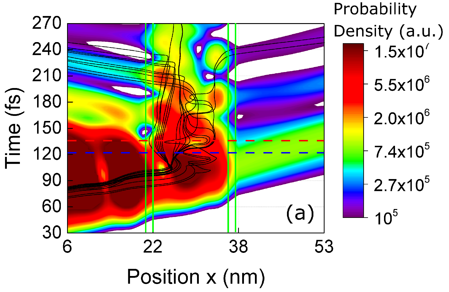
In Fig. 4(b) we plot the probability of the energy states $|c(E,t)|^{2}$ given by Eq. (20) at the two times indicated by horizontal read and blue dashed lines in Fig. 4(a) that corresponds to the vertical dashed lines in Fig 3. The BCWF in Eq. (20) has been defined as $\psi(x,t)=\Psi(x,Q^{j}[t],t)=\psi_{A}(x,t)\psi_{0}(Q^{j}[t])+\psi_{B}(x,t)\psi_{1}(Q^{j}[t])$ for a selected trajectory $Q^{j}[t]$ of the $j$-experiment. Notice that such definition of the BCWF corresponds in this case to $\psi(x,t)\approx\psi_{B}(x,t)$ for the blue wave packet, while the red wave packet corresponds to $\psi(x,t)\approx\psi_{A}(x,t)$, because of the values of $P_{A,2}$ and $P_{B,1}$ when Fig. 4(b) is estimated.

As expected, the fact that the conservation of the total energy has to be satisfied from (12) has important consequences on the type of electron-photon interaction allowed. We now repeat the simulation when the electron (with no photon) is injected with a central energy corresponding to the first resonant level. No electron transition (or spontaneous emission) takes place, giving $\psi_{B}(x,t)\approx 0$ because the initial energy $E_{1}+\hbar\omega/2$ cannot be converted into a much higher final energy $E_{2}+3\hbar\omega/2$. The result is shown in Fig. 5.

We now repeat the same simulation done in Fig 3, where the initial electron had mean energy equal to the second eigenvalue of the well, $E_{2}$, but considering a new photon energy $\hbar\omega=0.26$ eV much larger than $E_{2}-E_{1}=0.172$ eV. In this case no light-matter interaction takes place since it would imply a violation of the conservation of whole energy. The initial energy $E_{2}+\hbar\omega/2$ do not coincide with a possible final energy $E_{1}+3\hbar\omega/2$. This simulation is shown in Fig. 6.

In the previous subsection we discussed the interaction of a single electron with a single photon in a closed system. Here, we discuss how such interaction can be generalized to include the possibility to detect a photon at a position $y$, far from the active region.

The proper simulation of such scenario as a closed system is far from the scope of the present paper. Apart from considering the detector outside of the active region as a new electron with degree of freedom $y$, the transition of the electromagnetic energy from the active region to the environment will require an electromagnetic field with an arbitrary shape different from the one considered in the previous section. A Fourier transform of such arbitrary electromagnetic field will imply dealing with several components $E(x,t)\propto q\;cos(kx-\omega t)$ at different frequencies. In any case, without an explicit solution of such problem, only from the conservation of energy, we can anticipate what will be the expected behavior of the whole system.

The process of spontaneous emission of a photon inside the active region, and its posterior detection far from the active region, can be anticipated as:

• •

  At the initial time, $t=0$, we consider an electron in the active region, with degree of freedom $x$ with a central energy $E_{2}$, linked to zero photons wave function $\psi_{0}(q)$, plus another electron far from the active region, with degree of freedom $y$ and energy $E_{ext}$, linked to zero photons $\psi_{0}(q)$. At this initial time, thus, the total energy involved in such scenario is $E_{2}+\hbar\omega/2$, in the active region, plus the energy $E_{ext}+\hbar\omega/2$ outside.

• •

  At the intermediate time, we consider that a spontaneous emission of a photon happens inside the active region. As seen in Fig. 3, such internal process ensure energy conservation. So that the new photon inside the active region implies a change of energy there, $E_{2}+\hbar\omega/2\to E_{1}+3\hbar\omega/2$, while the energy outside of the active region remains the same as before, $E_{ext}+\hbar\omega/2$. The total energy is the same as the initial one.

• •

  At the final time $t$, we detect a photon at the position $y$ far from the active region. Thus, the electron at $y$ is now linked to one photon wave function $\psi_{1}(q)$ which implies an increment of the energy of $\hbar\omega$ far from the active region, $E_{ext}+\hbar\omega/2\to E_{ext}+3\hbar\omega/2$. The conservation of the total energy implies that the same amount of energy is eliminated in the active region when the photon is leaving it, $E_{1}+3\hbar\omega/2\to E_{1}+\hbar\omega/2$. The electron in the active region will have a new energy $E_{1}$ linked to the zero photons wave function $\psi_{0}(q)$. As we have seen in Fig. 5, under such new energy conditions in the active region, such electron will not be able any more to generate spontaneous emission inside the RTD. Thus, the Rabi oscillations seen in Fig. 3 for a closed system, will not be present when we assume that the photon is leaving the cavity.

In summary, using the BCWF to focus only on the description of the electron inside the active region as a single-particle pure state $\psi(x,t)$, we conclude that the spontaneous emission in the active region can be modeled by an initial BCWF $\psi(x,0)$ with central energy $E_{2}$ that changes to a final BCWF $\psi(x,t)$ with energy $E_{1}$. Such process will be allowed as far as the photon energy coincides with $E_{2}-E_{1}$. Identically, absorption in the active region can be modeled by an initial BCWF $\psi(x,0)$ with central energy $E_{1}$ that changes to a final BCWF $\psi(x,t)$ with energy $E_{2}$ with the photon energy given by $E_{2}-E_{1}$. The conservation of energy enables the photon absorption to be accompanied by a subsequent process of spontaneous emission, that returns the photon energy to the environment outside of the active region.

We consider an electron defined by a single-particle BCWF that at time $t_{s}$ undergoes a scattering event. We define $t_{s}^{-}=t_{s}-\Delta t_{s}$ as the time just before and $t_{s}^{+}=t_{s}+\Delta t_{s}$ as the time just after the scattering event. For simplicity, we consider $\Delta t_{s}\to 0$, but we have seen in Sec. 3 that such transition between initial and final BCWF takes a finite time because, from a conceptual point of view, it has to guarantee the continuity of the BCWF in space and time. The initial and final BCWFs are $\psi(x,t_{s}^{-})$ and $\psi(x,t_{s}^{+})$, which satisfy $\langle E(t_{s}^{+})\rangle=\langle E(t_{s}^{-})\rangle+E_{\gamma}$, with $E_{\gamma}$ the energy of a photon. Within the energy representation, the wave packet can be decomposed into a superposition of Hamiltonian eigenstates $\phi_{E}(x)$ of the electron $\hat{H}_{e}$ in (8) as

$$\psi(x,t_{s^{-}})=\int dE\;a(E,t_{s}^{-})\;\phi_{E}(x),$$

(23)

with $a(E,t)=\int dx\;\psi(x,t)\;\phi_{E}^{*}(x)$. The central energy $\langle E(t_{s}^{-})\rangle$ is

$$\langle E(t_{s}^{-})\rangle=\int dE\;E\;|a(E,t_{s}^{-})|^{2},$$

(24)

which can be increased to get the new central energy at $t_{s}^{+}$ as

	$\displaystyle\langle E(t_{s}^{+})\rangle$	$\displaystyle=$	$\displaystyle\langle E(t_{s}^{-})\rangle+E_{\gamma}$		(25)
		$\displaystyle=$	$\displaystyle\int dE\;(E+E_{\gamma})\;|a(E,t_{s}^{-})|^{2}$
		$\displaystyle=$	$\displaystyle\int dE^{\prime}\;E^{\prime}\;|a({E^{\prime}-E_{\gamma}},t_{s}^{-})|^{2}$
		$\displaystyle=$	$\displaystyle\int dE^{\prime}\;E^{\prime}\;|a^{\prime}(E^{\prime},t_{s}^{+})|^{2},$

where we have defined $a^{\prime}(E,t_{s}^{+})=a(E-E_{\gamma},t_{s}^{-})$. Thus, the new wavepacket after the collision is

	$\displaystyle\psi(x,t_{s^{+}})$	$\displaystyle=$	$\displaystyle\int dE\;a^{\prime}(E,t_{s}^{+})\;\phi_{E}(x)$		(26)
		$\displaystyle=$	$\displaystyle\int dE\;a(E^{\prime}-E_{\gamma},t_{s}^{-})\;\phi_{E}(x).$

This transition corresponds to absorption of energy by the electron. Emission can be identically modeled by using $\langle E(t_{s}^{+})\rangle=\langle E(t_{s}^{-})\rangle-E_{\gamma}$. If required, the technical discontinuity between $\psi(x,t_{s^{-}})$ and $\psi(x,t_{s^{+}})$ can be solved by just assuming that the change of energy is produced in a finite time interval $\Delta t_{s}=N_{t_{s}}\Delta t$, with $\Delta t$ the time step of the simulation. Then, at each time step of the simulation, the change in the wave packet central energy is $E_{\gamma}/N_{t_{s}}$. A continuous change of both energy and wave packet will be obtained as far as $\Delta t\to 0$.

This continuous evolution of the BCWF can be represented as a Schrödinger-like equation as explained in [31]. In any case, the shape of the Hamiltonian of this new Schrödinger equation describing the collision is subjected to the post-selection of the state.

In Ref. [34] we explain how a change of momentum $p_{\gamma}$ in a wave packet in free space can be performed with a unitary Schrödinger equation. That algorithm can be understood as a pre- and a post-selection of the initial BCWF, $\psi(x,t_{s}^{-})$, and of the final BCWF, $\psi(x,t_{s}^{+})$, respectively. At time $t_{s}^{-}$, the BCWF can be written as a superposition of momentum eigenstates $\phi_{p}(x)$ (which are a basis of the electron in the x space) as

$$\psi(x,t_{s^{-}})=\int dp\;b(p,t_{s^{-}})\;\phi_{p}(x),$$

(27)

with $b(p,t_{s^{-}})=\int dx\psi(x,t_{s^{-}})\;\phi_{p}^{*}(x)$. The central momentum $\langle p(t_{s}^{-})\rangle$ is

$$\langle p(t_{s}^{-})\rangle=\int dp\;p\;|b(p,t_{s^{-}})|^{2},$$

(28)

which can be increased to get the new central momentum $\langle p(t_{s}^{+})\rangle=\langle p(t_{s}^{-})\rangle+p_{\gamma}$ at $t_{s}^{+}$ as

	$\displaystyle\langle p(t_{s}^{+})\rangle$	$\displaystyle=$	$\displaystyle\langle p(t_{s}^{-})\rangle+p_{\gamma}$		(29)
		$\displaystyle=$	$\displaystyle\int dp\;(p+p_{\gamma})\;|b(p,t_{s^{-}})|^{2}$
		$\displaystyle=$	$\displaystyle\int dp^{\prime}\;p^{\prime}\;|b({p^{\prime}-p_{\gamma}},t_{s^{-}})|^{2}$
		$\displaystyle=$	$\displaystyle\int dp^{\prime}\;p^{\prime}\;|b(p^{\prime},t_{s^{+}})|^{2},$

where we have defined $b(p,t_{s^{+}})=b(p-p_{\gamma},t_{s^{-}})$. In this particular scenario, we know the explicit shape of the momentum eigenstates, $\phi_{p}(x)=1/\sqrt{2\pi}\exp(ipx/\hbar)$, so that

	$\displaystyle\psi(x,t_{s}^{+})$	$\displaystyle=$	$\displaystyle\int dp\;b(p,t_{s^{+}})\;\phi_{p}(x)$		(30)
		$\displaystyle=$	$\displaystyle\int dp\;b(p-p_{\gamma},t_{s^{-}})\;\phi_{p}(x)$
		$\displaystyle=$	$\displaystyle\int dp\int dx^{\prime}\psi(x,t_{s^{-}})\;\phi_{p-p_{\gamma}}^{*}(x^{\prime})\phi_{p}(x)$
		$\displaystyle=$	$\displaystyle\int dp\int dx\;\psi(x,t_{s^{-}})\;\frac{1}{2\pi}e^{ip(x^{\prime}-x)/\hbar}e^{ip_{\gamma}x^{\prime}/\hbar}$
		$\displaystyle=$	$\displaystyle e^{ip_{\gamma}x/\hbar}\psi(x,t_{s^{-}}).$

With the condition $\psi(x,t_{s}^{+})=e^{ip_{\gamma}x/\hbar}\psi(x,t_{s^{-}})$, it can be easily demonstrated which one is the unitary equation satisfied by the BCWF. If we define $\psi^{\prime}(x,t)$ as the wave function solution of the following Schrödinger equation, $i\hbar\frac{\partial\psi^{\prime}(x,t)}{\partial t}=\frac{1}{2m^{*}}\left(-i\hbar\frac{\partial}{\partial_{x}}\right)^{2}\psi^{\prime}(x,t)+V(x)\psi^{\prime}(x,t)$, with initial condition at $t=t_{s}$ given by $\psi^{\prime}(x,t_{s})=\psi(x,t_{s}^{+})$, then, the solution $\psi^{\prime}(x,t)$ for $t>t_{s}$ is identical to the following Schrödinger equation, $i\hbar\frac{\partial\psi(x,t)}{\partial t}=\frac{1}{2m^{*}}\left(-i\hbar\frac{\partial}{\partial_{x}}+p_{\gamma}\right)^{2}\psi(x,t)+V(x)\psi(x,t)$, for the original $\psi(x,t)$ and with its original initial condition for $t>t_{s}$. Finally, a single equation for $\psi(x,t)$ valid for all times is just

	$\displaystyle i\hbar\frac{\partial\psi(x,t)}{\partial t}$	$\displaystyle=$	$\displaystyle\frac{1}{2m^{*}}\left(-i\hbar\frac{\partial}{\partial_{x}}+p_{\gamma}\Theta_{t_{s}}\right)^{2}\psi(x,t)$		(31)
		$\displaystyle+$	$\displaystyle V(x)\psi(x,t),$

where $\Theta_{t_{s}}$ is a Heaviside function equal to $1$ for $t>t_{s}$ and zero otherwise. Thus, a description of the evolution of the wave function $\psi(x,t)$ during the collision process can be done from a unitary Schrödringer equation, where the momentum operator $-i\hbar\frac{\partial}{\partial_{x}}$ is changed for the new momentum operator $-i\hbar\frac{\partial}{\partial_{x}}+p_{\gamma}\Theta_{t_{s}}$, as indicated in [34]. Notice that the probability presence of the scattered wave packet satisfies $|\psi(x,t_{s^{+}})|^{2}=|\psi(x,t_{s^{-}})|^{2}$ because only a global phase $e^{ip_{\gamma}x/\hbar}$ is added.

References

- [1] Breuer, H. P.; Petruccione, F. Theory of Open Quantum Systems, Oxford University Press, Oxford, 2002; pp. 5-23.
- [2] Klimeck, G. Single and multiband modeling of quantum electron transport through layered semiconductor devices. Journal of Applied Physics 1997, 81, 7845.
- [3] Klimeck, G.; Ahmed, S.S.; Bae, H.; Kharche, N.; Clark, S.; Haley, B.; Lee, S.; Naumov, M.; Ryu, H.; Saied, F.; Prada, M.; Korkusinski, M.; Boykin, T.B. Atomistic Simulation of Realistically Sized Nanodevices Using NEMO 3-D Part I: Models and Benchmarks. IEEE Trans. on El. Dev., 2007, 54, 9, 2079-2089.
- [4] Schmidt, A.; Cheng, B.; daLuz, M. Green function approach for general quantum graphs. J. of Phys. A 2003, 36, 42.
- [5] Rossi, F. The Density-Matrix Approach Theory of Semiconductor Quantum Devices. NanoScience and Technology Springer, Berlin, Heidelberg, 2010, pp. 89-130.
- [6] Iotti, C.; Ciancio, E.; Rossi, F. Quantum transport theory for semiconductor nanostructures: A density-matrix formulation. Phys. Rev. B 2005, 72, 125347.
- [7] Wigner, E.P. On the quantum correction for thermodynamic equilibrium. Phys. Rev. 1932, 40, 5, 749–759.
- [8] Frensley, W.; Wigner-Function Model of Resonant-Tunneling Semiconductor Device. Phys. Rev. B, 1987, 36, 3, 1570–1580.
- [9] Weinbub, J.; Ferry, D. K. Recent advances in Wigner function approaches. Appl. Phys. Rev., 2018, 5, 041104.
- [10] Querlioz, D.; Huu-Nha Nguyen; Saint-Martin, J. ; Bournel, A.; Galdin-Retailleau, S.; Dollfus, P. Wigner-Boltzmann Monte Carlo approach to nanodevice simulation: from quantum to semiclassical transport. Journ. of Comp. El., 2009, 8, 324–335.
- [11] Nedjalkov, M.; Querlioz, D.; Dollfus, P.; Kosina, H.; Wigner Function Approach. Nano-Electronic Devices, Springer, 2011, pp. 289–358.
- [12] Fan, Z.; Garcia, J.; Cummings, A.; Barrios-Vargas, J.; Panhans, M.; Harju, A.; Ortmann, F.; Roche, S. Linear scaling quantum transport methodologies. Physics Reports 2020, available online.
- [13] Vyas, P.; Van de Put, M.; Fischetti, M. Master-Equation Study of Quantum Transport in Realistic Semiconductor Devices Including Electron-Phonon and Surface-Roughness Scattering. Phys. Rev. Applied 2020, 13, 014067.
- [14] Fischetti, M. Theory of electron transport in small semiconductor devices using the Pauli master equation, J. of Appl. Phys. 1998, 83, 270.
- [15] Kramer, T.; Kreisbeck, C.; Krueckl, V. Wave packet approach to transport in mesoscopic systems, Physica Scripta 2010, 82, (3), 038101.
- [16] Bracher, C.; Delos, J.; Kanellopoulos, V.; Kleber, M.; Kramer, T. The photoelectric effect in external fields. Phys. Lett. A 2005, 347, 1-3, 62-66.
- [17] Bohm, D. A Suggested Interpretation of the Quantum Theory in Terms of ”Hidden” Variables. Phys. Rev. 1952, 85, 166.
- [18]
Bohmian Interacting Transport in non-equiLibrium eLEctronic Structures (BITLLES).
Simulator available online: http://europe.uab.es/bitlles. - [19] Vacchini, B.; Smirne, A.; Laine, E.; Piilo, J.; Breuer, H. Markovianity and non-Markovianity in quantum and classical systems, New J. of Phys. 2011, 13, 093004.
- [20] Lindblad, G. On the generators of quantum dynamical semigroups. Commun. Math. Phys. 1976, 48, 119-130.
- [21] Ferialdi, L. Exact Closed Master Equation for Gaussian Non-Markovian Dynamics. Phys. Rev. Lett. 2016, 116, 120402.
- [22] Vega, I.; Alonso, D. Dynamics of non-Markovian open quantum systems. Rev. Mod. Phys. 2017, 89, 015001.
- [23] Ghirardi, G.C.; Rimini, A.; Webber, T. Unified dynamics for microscopic and macroscopic systems. Phys. Rev. D 1986, 34, 470.
- [24] Bassi, A.; Lochan, K.; Satin, S.; Singh, T.P.; Ulbricht, H. Models of wave-function collapse, underlying theories, and experimental tests. Rev. Mod. Phys. 2013, 85, 471.
- [25] Strunz, W.T.; Diósi, L.; Gisin, N. Open System Dynamics with Non-Markovian Quantum Trajectories. Phys. Rev. Lett. 1999, 82, 1801.
- [26] Strunz, W.T. The Brownian motion stochastic Schrödinger equation, Chem. Phys. 2001, 268, 237.
- [27] Ferialdi, L.; Bassi, A. Exact Solution for a Non-Markovian Dissipative Quantum Dynamics, Phys. Rev Lett. 2012, 108, 170404.
- [28] Gambetta, J.; Wiseman, H.M. Non-Markovian stochastic Schrödinger equations: Generalization to real-valued noise using quantum-measurement theory. Phys. Rev. A 2002, 66 012108.
- [29] Gambetta, J.; Wiseman, H.M. The interpretation of non-Markovian stochastic Schrödinger equations as a hidden-variable theory. Phys. Rev. A 2003, 68 062104.
- [30] Diósi, L.; Ferialdi, L. General Non-Markovian Structure of Gaussian Master and Stochastic Schrödinger Equations. Phys. Rev. Lett. 2014, 113 200403.
- [31] Oriols, X. Quantum-Trajectory Approach to Time-Dependent Transport in Mesoscopic Systems with Electron-Electron Interactions. Phys. Rev. Lett. 2007, 98, 6, 066803.
- [32] Dürr, D.; Teufel, S. Bohmian Mechanics: The Physics and Mathematics of Quantum Theory Springer, Berlin, 2009.
- [33] Oriols, X.; Mompart, J. Applied Bohmian Mechanics: From Nanoscale Systems to Cosmology, 2nd ed., Jenny Stanford Publishing: Singapore, 2019.
- [34] Colomés, E.; Zhan, Z.; Marian, D.; Oriols, X. Quantum dissipation with conditional wave functions: Application to the realistic simulation of nanoscale electron devices. Phys. Rev. B 2017, 96, 7, 075135.
- [35] Albareda, G.; López, H.; Cartoixà, X.; Suñé, J.; Oriols, X. Time-dependent boundary conditions with lead-sample Coulomb correlations: Application to classical and quantum nanoscale electron device simulators. Phys. Rev. B 2010, 82 085301.
- [36] Marian, D.; Colomés, E.; Oriols, X. Quantum noise from a Bohmian perspective: fundamental understanding and practical computation in electron devices. J. Phys. Condens. Matter 2015, 27 245302.
- [37] Albareda, G.; Traversa, F. L.; Benali, A.; Oriols, X. Computation Of Quantum Electrical Currents Throught The Ramo–Shockley–Pellegrini Theorem With Trajectories Fluctuation and Noise Letters, 2012, 11, 03, 1242008,
- [38] Jacoboni, C.; Reggiani, L. The Monte Carlo method for the solution of charge transport in semiconductors with applications to covalent materials. Rev. Mod. Phys. 1983, 55 645.
- [39] Tzemos, A. C.; Contopoulos, G.; Efthymiopoulos, C. Bohmian trajectories in an entangled two-qubit system. Phys. Scr. 2019, 94 105218.
- [40] Tzemos, A. C.; Contopoulos, G. Chaos and ergodicity in an entangled two-qubit Bohmian system. Phys. Scr. 2020, 99, 6, 065225.