On the Number of Graphs with a Given Histogram
Abstract
Let be a large (simple, unlabeled) dense graph on vertices. Suppose that we only know, or can estimate, the empirical distribution of the number of subgraphs that each vertex in participates in, for some fixed small graph . How many other graphs would look essentially the same to us, i.e., would have a similar local structure? In this paper, we derive upper and lower bounds on the number of graphs whose empirical distribution lies close (in the Kolmogorov-Smirnov distance) to that of . Our bounds are given as solutions to a maximum entropy problem on random graphs of a fixed size that does not depend on , under global density constraints. The bounds are asymptotically close, with a gap that vanishes with at a rate that depends on the concentration function of the distribution at the center of the Kolmogorov-Smirnov ball.
1 Introduction
Let be a simple unlabeled dense graph on vertices. Suppose that we cannot access the entire graph, which could be very large, but we are nevertheless interested in gaining some information about its local structure. To that end, we could for instance randomly query a small number of vertices, and probe their local neighborhoods. For example, if we record the degrees of these random vertices, we can obtain a coarse estimate of the degree distribution of the graph, which we can think of as a histogram of the true underlying (empirical) degree distribution. Similarly, we can obtain a histogram of the distribution of the number of triangles a vertex participates in. Or more generally, fixing any rooted graph on vertices, we can obtain a histogram of the -degree distribution of , i.e., of the number of times a vertex in appears as the root of a subgraph . We will refer to this as an -histogram of . Given such an -histogram, how much is revealed about the graph itself? More concretely, we are interested in characterizing the number of graphs whose -histogram is similar to that of .
Contribution and techniques. In this paper, we formalize the above question in a more abstract manner, by defining a histogram as a ball in the Kolmogorov-Smirnov (KS) metric around some smooth reference distribution. We then characterize the number of graphs whose true -degree distribution lies inside the ball, in terms of a solution to a constrained maximum entropy problem over fixed-dimension random graphs. Our approach is based on the following ideas. First, we show that the local structure conditions can be essentially replaced by global ones with only a small penalty; loosely speaking, we show that the set of graphs with -degree distribution inside a KS-ball roughly correspond to a set of graphs satisfying certain global density constraints w.r.t. graphs derived from , where by density we mean the relative occurrence of each inside . This reduction to vector of densities is obtained by counting arguments combined with an anti-concentration inequality.
Given this reduction, it is enough to characterize the number of graphs with (roughly) a given density vector. To that end, and in a way somewhat reminiscent of the method-of-types [1], we define something we call a Szemerédi type of a graph. A Szemerédi type is essentially a random graph over vertices with edges drawn independently with probabilities , together with some accuracy parameter . Loosely speaking, a graph on vertices is said to have this Szemerédi type, if we can partition (most of) its vertex set into equi-sized parts, such that the edges between parts and appear to have been drawn independently at random with probability , as long as we do not look too closely (determined by ). In general, a graph can have no Szemerédi type, or can have multiple Szemerédi types. The celebrated Szemerédi regularity lemma [2] implies that for large enough, every graph has at least one Szemerédi type, and hence one can roughly think of large enough graphs as being “pseudorandom” with a small number of parameters. We use this fact in order to convert our vector of densities problem into an optimization problem over (fixed dimension) Szemerédi types, and show that its solution is essentially given by the Szemerédi type with maximum entropy satisfying the corresponding expected density constraints. The gap between our upper and lower bounds depends on the number of density constraints we take, and vanishes at a rate that depends on the concentration function of the distribution at the center of our KS-ball.
Motivation. Graphs are widely used to describe relations between different elements in a system, with notable examples including computer networks, social media, molecular structures and biological systems. Moreover, often these large networks have a typical underlying structure, such as edge-degree distribution (as observed e.g., for the Internet [3]) or triangle-degree distribution (e.g., the edge-triangle configuration model [4, 5]), and more generally, -degree distribution [6, 7, 8]. While our work addresses a fundamental combinatorial question regarding the number of graphs with a certain distribution of local properties, it is primarily motivated by the need to provide a combinatorial framework for information theoretical problems over large graphs, in the spirit of the well-known typicality [9] and method-of-types [1] used for sequences.
In the method-of-types, the basic idea is to characterize a finite sequence by the empirical distribution of its symbols, referred to as the type of the sequence, and then quantify the number of sequences with the same type, which turns out to be exponential in the entropy of the type. This very simple idea goes a very long way in information theory both in data compression and communication, see [1]. In our setting, the simple sequence type is replaced by a graph -histogram (that can be computed using one of the various existing subgraph listing or subgraph local counting algorithms, e.g., [10, 11, 12, 13, 14, 15, 16]), or more generally and loosely speaking, by a Szemerédi type. In a way analogous to the classical result for sequences, the entropy of the Szemerédi type will yield the correct exponential behavior of the number of graphs that share the underlying histogram(s), with the small but important distinction that we allow a small deviation (in the KS metric). Hence our result in this sense is more reminiscent of sequence typicality [9] (we later discuss why exact counting is nontrivial in the graph setup, in contrast to the sequence setup). Just as in the sequence case, this immediately leads to a lossless compression result, describing the minimal number of bits required in order to represent a graph with a given histogram so that it can be exactly reconstructed. Furthermore, again as in the sequence case, this type of fundamental characterization can be leveraged to address more difficult information-theoretic questions.
One such interesting example is structure-preserving lossy compression of graphs. It has been long observed [17] that the global properties of a graph, e.g., edge probability and subgraph counts, are not enough in order to describe realistic networks. Local properties, such as the clustering coefficient and the small world property are required [17, 18]. These properties measure the dependence between the edge probability of two vertices and their joint neighborhood. For example, large clustering coefficient suggests that if two vertices have many joint neighbors, they are likely to have an edge between them. Therefore, preserving the local neighborhood of each vertex in the compression process can be desirable. If one uses a global distortion measure, as, say, the Hamming distance, then even a very small overall distortion (i.e., edges removed or added) can concentrate on a small subset of vertices or even erase a specific neighborhood entirely. This can be prevented by using a measure that controls the local distortion. In this type of a setting, we are given a large graph, and would like to represent it using the minimal number of bits, while preserving some local structure up to some prescribed distortion, for each and every vertex (e.g., the set of actual triangles in which each vertex participates in the original graph and its reconstruction, should have say a overlap). This type of problem was previously considered in [19] for the edge case, by using known results on edge-degree counts [20, 21], see Section 2 for further details. In order to generalize this method for measures that control the -degree distortion for general , results on the number of graphs with (approximately) the same histogram, which we give here, appear to be required.
Organization. Section 2 reviews relevant previous results and related work. Section 3 includes some necessary preliminaries and definitions. In Section 4 we formally present the graph histogram characterization problem and state our main results. In Section 5 we introduce the Szemerédi types, which play a central role in our proofs. Then, in Section 6 we prove our main result in two steps: First, in Subsection 6.1, we reduce the histogram characterization problem to a vector subgraph densities problem via anticoncentration arguments. Then, in Subsection 6.2, we resolve the densities problem via Szemerédi types and the regularity lemma, thereby yielding our main result. In Section 7, we slightly digress to examine the subgraph densities problem in the special case of a scalar density; unlike the general vector setting, this case admits a simple finite expression. Finally, in Section 8, we conclude by discussing some gaps as well as possible extensions of our work. Additional background and some technical proofs are relegated to the Appendix.
2 Related work
The case of edge-degree distributions, where is a single edge on vertices, was solved by Barvinok [20, 21], who used a generating functions approach to show that the number of graphs with a given degree distribution is obtained as a solution to an -parameter maximum entropy problem. Compared to our approach, his result is stronger as it yields the number of graphs (up to sub-exponential terms) that have the exact given edge-degree distribution, rather than close in the KS metric, albeit his solution involves dimensional optimization rather than dimensional in our case (but this can of course be fixed). Recently, the authors gave a simpler information-theoretic proof for Barvinok’s result by leveraging degree-distribution invariant operations [22]. Later in [23, 19], these results were used to derive bounds on the rate distortion function for universal lossy compression of directed random graphs, under distortion measure that limits the number of edges one vertex can lose or gain in the compression process. The degree sequence of graphs was also studied in [24], were it was shown that sequences of graphs with a given degree sequence converge to a unique, identifiable limiting object. We elaborate on this limiting object, called a graphon, in Subsection 2.1.
The general case of -degree distributions or -histograms has not been addressed before, and it appears that both the approaches used by Barvinok and the authors are not easy to extend. The difficulty of going beyond the edge case is underscored by the feasibility problem, i.e., checking whether the set of graphs with a given -degree distribution is nonempty. The feasibility problem is resolved by the Gale-Ryser Theorem [25, 26] in the edge case, but is not well understood for general . This is also another reason to work with -histograms rather than exact -degree distributions.
The problem of characterizing the number of graphs with an approximately given scalar graph parameter (as defined later), in the limit of , was addressed by Chatterjee and Varadhan [27] using an object called a graphon[28], that can be loosely thought of as a compact limit of Szemerédi types for . They derived a large deviation result that yields upper and lower bounds on the exponent of the size; in particular relevance to our setting, they showed that their bounds coincide when the graph parameter is a scalar subgraph density, yielding a size exponent given by the maximum entropy graphon satisfying the single density constraint. In [29], these results were used to approximate the normalizing constant of exponential random graph models with subgraph counts as their sufficient statistics. In [30], Lubetzky and Zhao studied related problems via the regularity lemma lens, and in particular gave a more general sufficient condition on the scalar parameter for the bounds to coincide. These works however do not readily generalize to the vector densities case, as outlined in the next subsection (which can be skipped without affecting the rest of the paper).
2.1 Graphons and the Chatterjee-Varadhan (CV) Large Deviation Bounds
In a sequence of papers (see [28] and references therein), Lovaśz et al. developed a beautiful theory of graph limits, and introduced the notion of graphons. A graphon is a measurable function that satisfies . The space of graphons (up to measure preserving bijections) can be endowed with a metric called the cut metric (see Appendix A.1). Any graph on vertices can be represented as a “checkerboard” graphon , where
| (1) |
A graph parameter is a (scalar or vector) function that can be extended to a continuous (w.r.t to the cut metric) function over graphons, such that . Graphons become useful in the context of graphs due to the following property: Let be a sequence of simple graphs over vertices, and let denote the relative occurrence of in (a formal definition of will later appear). Then, if for any fixed the sequence converges as , the sequence converges to a graphon , in the sense that converges to in the cut metric.
Chatterjee and Varadhan used Lovász’s graphon framework to derive a large deviation result [27, Theorem 2.3] that gives bounds on the number of graphs whose parameter lies inside a given set, in the limit of large . Their bounds (stated explicitly in Appendix A.1) are given as a maximum entropy problem over a set of graphons that satisfy the associated constraints on their corresponding graph parameter. The lower bound corresponds to the maximum over the set of graphons whose parameter value lies within an open set, and the upper bound correspond to the maximum over the set of graphons whose parameter value lies within the closure of that set. Formal definitions and the explicit bounds can be found in Appendix A.1.
The aforesaid CV large deviation result is quite general and can be applied to various graph parameters, scalar or vector, as also remarked by the authors in [27]. However, it is important to note that the resulting bounds are not generally tight; namely, the upper and lower CV bounds coincide in some cases but not in others. Specifically, the CV bounds are not tight in the case where the maximum entropy solution is not continuous w.r.t the parameter level. If an infinitesimally small change in the value of the parameter that defines the feasible set of graphons can cause a large change in the corresponding maximum entropy, a jump discontinuity will occur at the boundary of (some) closed set that defines the CV upper bound, thus strictly separating it from the CV lower bound. An explicit (toy) example of a scalar graph parameter for which the bounds are not tight can be found in Appendix A.1. In the special case where the parameter is the -density of the graph, , the bounds are indeed tight and thus yielding (asymptotically) the exact exponential count of the number of graphs with -density inside a given interval.
The above tightness issue has been addressed in [30], in the scalar parameter case. A graph parameter is called nice when all its local extrema are also global ones. The authors in [30] showed that the CV bounds (applied e.g. to an open interval and its closure) are tight for all (scalar) nice graph parameters. Specifically, define the rate function as the solution to a maximum entropy problem
| (2) |
where
| (3) |
and is the binary entropy function. Then being nice implies that the rate function is continuous in , which is a necessary and sufficient condition for the bounds to be tight. The -density of the graph was shown to be nice in [30], and in fact the continuity of in this case has already been implicitly used by Chatterjee and Vardahn in the proof of [27, Theorem 4.1].
To the best of our knowledge, there has been no prior work giving conditions for the tightness of the CV bounds in the case that is a vector parameter. The difficulty in this case is to generalize the notion of maxima and minima to vectors in a way that yields a property equivalent to niceness in the scalar case. Part of our contribution here is to suggest a generalization of niceness in multiple dimensions; we do so by defining local and global boundary points (formally introduced in Subsection 6.2) and requiring that every local boundary point is also a global one. However, this property is difficult to generally establish, as discussed also in Subsection 6.2. We circumvent this issue by defining a local measure of niceness, the effective radius, in a finite setup, which will imply that there are no boundary points in a specific neighborhood (in the Szemerédi types space).
In fact, it should be further stressed that niceness of the parameter (in both the scalar and vector cases) is not sufficient in our setup, since we are interested in a finite characterization. The CV bounds work on asymptotical objects (graphons), and do not immediately yield finite bounds. In order to obtain such bounds, one needs to use the Szemerédi regularity lemma, and then a suitable counting lemma. The resulting bounds are then given as maximum entropy problems over sets of Szemerédi types. Then, loosely speaking, in order for the bounds to be tight we need the maximum entropy Szemerédi type of the lower and upper bounds not to be too far apart. This requires, in addition to continuity of the maximum entropy solution with respect to the parameter level, also some quantitative result bounding the gradient of the mapping , as further elaborated in Subsection 6.2.
We remark that as observed in [31], the CV large deviation bounds coincide for any graph parameter (scalar or vector) in the case where one is only interested in the asymptotic size exponent for an exact level of the graph parameter. This asymptotic exponent was studied in [31] for the edge-triangle case, and later generalized in [32] to a vector of -star densities. While this type of analysis is insightful and interesting, it should be noted that the resulting asymptotic size exponents have no operational meaning due to order of limits (first in , and then in the ball size around the parameter level). For instance, it could be that there exist no graphs (for any ) at certain parameter value (e.g., irrational density) but the asymptotic size exponent is still nontrivial. To obtain operational results, the graph parameter must therefore satisfy the above mentioned continuity properties. Furthermore, these properties need to hold in a stronger sense in order to obtain a finite characterization, which is necessary for example in applications such as lossy and lossless compression of graphs discussed in Section 1, and is the approach we take here.
3 Preliminaries and Notation
The Kolmogorov-Smirnov (KS) distance between two probability distributions and over , is the distance between c.d.f.s, i.e.,
| (4) |
The concentration function of returns the maximal probability that gives to any interval of a given size, i.e.,
| (5) |
We use boldface letters to indicate vectors and write for to mean an entry–wise inequality. In this work, all graphs are simple, undirected, and unlabeled, unless otherwise noted. For a graph we denote by the set of all vertices in . We write for two vertices to mean that there is an edge between and in . The collection of all graphs on vertices is denoted by . For a random graph the notation means that has independent edges and the edge exists with probability . If is a matrix then we denote by the element in the th row and th column. In all the following we use the natural base for the log function.
4 Problem Setting and Main Result
Let be a graph on vertices. Let be a graph on vertices, where one of the vertices is designated as the root vertex. We say that a vertex of has -degree , if appears as the root vertex in exactly copies of in . Loosely speaking, a copy is any appearance of inside , counted once. Precisely, a copy is an element in the quotient set , where is the set of all injections such that in implies in , and is an equivalence relation on where are equivalent if for some from the automorphism group of .
Define the -degree distribution of the graph to be the empirical distribution of the vertices -degrees, i.e.,
| (6) |
Furthermore, define normalized -degree distribution , obtained from by normalizing the latter to have support in . Namely, letting denote the -degree of a vertex in the complete graph on vertices (which is the maximal possible), then with implies . For example, if is a clique of size we have .
For any distribution with support in , we define the -histogram as the set of all graphs on vertices, whose normalized -degree distribution is -close to in KS distance, i.e.,
| (7) |
From here on, we suppress and write to denote . In what follows, we will be interested in characterizing the -histogram size. Specifically, we will show that the logarithm of the -histogram size is approximately equal to the entropy of a random graph with independent edges on vertices, where the maximization is subject to suitable subgraph density constraints.
To that end, define the -density of a graph to be
| (8) |
where is the number of copies of in the complete graph on vertices. The -density of a random graph can be defined similarly, to be (roughly) the expected fraction of appearances of in ; the exact expression for the mean density, which is a polynomial in , is discussed later in Section 5. Given an indexed family of small graphs we write to denote the corresponding vector of -densities. Let , and define
| (9) |
where . Namely, is the maximal possible (per-edge) entropy of a random graph on vertices, with -densities that are -close to .
Our main result shows that for a specific choice of , and , the function gives upper and lower bounds on the -histogram size. To state our result, we need a few more definitions. First, let be a graph on vertices obtained by taking disjoint copies of , and merging their root vertices into a single joint root vertex. Now, fixing some and the graph , let
| (10) |
Furthermore, set some reference distribution and let , and have entries
| (11) |
where
| (12) |
and is the size of the automorphism group of . The limit (12) exists since and are polynomials of the same degree in . We later show that approximates the -density of with error. We will also show that the -distance between two distributions can be bounded in terms of the closeness of their first moments (and therefore in terms of , ), thus translating the -degree distribution constraint to global density constraints.
We are now ready to state our main result. For better readability, we omit some technical details at this point, and provide them later in Subsection 6.2 (see Theorem 2).
Theorem 1.
Let be a distribution on that is absolutely continuous w.r.t. the Lebesgue measure, with a density bounded away from zero and infinity. Then, under some regularity conditions, for and any sufficiently large ,
where and , and means up to some vanishing (with ) error terms.
5 Szemerédi Types
We begin by defining two important entities: a -uniform partition of a graph and a Szemerédi type of a graph. We will later use these notions in Subsection 6.2 when we solve the maximum entropy problem with density constrains. Let be a graph and be a pair of disjoint subsets. The density of the pair is the fraction where is the number of edges with one endpoint in and second in and denote the cardinalities of and , respectively. The pair is called -uniform if for every , , , , it holds that . A partition is called -uniform if
- 1.
.
- 2.
.
- 3.
all but of the pairs are -uniform.
A Szemerédi type is a triplet , where , , and is a symmetric matrix with entries in . We say that a graph has Szemerédi type if there exists some -uniform partition of and for . From hereon we denote . We will loosely refer to the matrix as a -Szemerédi type, or simply a Szemerédi type, when are clear from context. The Szemerédi type class is defined as the collection of all graphs on vertices for which is a -Szemerédi type. We will sometimes write when are clear from context.
Note that a graph can have multiple -Szemerédi types, or none at all. The following well-known lemma shows that when is sufficiently large, at least one such type exists.
Lemma 1 (Szemerédi regularity lemma [2]).
For any , there exist positive integers , and , , such that every graph with at least vertices has at least one -Szemerédi type.
We remark that the in the above lemma is usually very large. It is easily lower bounded by , but is in fact much larger; the best known upper bound is a tower of exponentials of height proportional to [2], and this cannot be significantly improved [33]. However, the important point is that is a function of only, and does not depend on .
A Szemerédi partition is essentially a coarse partition of the vertex set that “looks random”. A Szemerédi type therefore naturally corresponds to a random graph over vertices, and we can think of as essentially being the probability of seeing a copy of when looking at uniformly random vertices of the random graph . More accurately, let be uniformly distributed over , and be a graph with vertex set , where in if and only if and in . Then, we define
| (13) |
Note that the above extends the deterministic subgraph density (8), with the small (but significant) distinction of allowing multiple drawings of the same vertex. The exact expression of is a polynomial of degree at most . In the simple case that is clique it is given by
| (14) |
To generalize the above to non-cliques, we need some adjustments. Now, vertices in that are not connected with an edge between them can be chosen in the same set . Hence, the mean -type depends on all the different possible proper vertex colorings of . A proper vertex coloring of a graph is a labeling of the graph’s vertices with colors such that no two vertices sharing the same edge have the same color. We define by the set of all proper coloring of . Then, denotes the number of different colors in the coloring , and we have that , where is the chromatic number of . The occurrence vector of a coloring , is a vector of length whose th entry records the number of vertices that has the th color in the coloring. We call two coloring different if their corresponding occurrence vectors are not equal in some coordinate. Define the mean -density of a -Szemerédi type to be
where is the size of the automorphism group of . In the above, the outer sum is over all the possible sizes , of coloring of , and the inner sum runs over all the proper coloring with size .
In Lemma 6, we will show that all graphs have -density that is approximately equal to , and moreover, have bounded deviation from this average quantity.
6 Proof of Main Result
Let be a family of graphs. Let . Then, the -densities set , is the set of all graphs on vertices whose -densities vector is -close to , i.e.,
| (15) |
Recall the specific definition of the family in (10), induced by a single graph . The first step in proving our main result is showing that for defined in (11), there exist a choice of and , such that . This will be done in Subsection 6.1. Then, in Subsection 6.2 we give sufficient conditions on under which the size of the set is (asymptotically) equal to the maximum entropy solution given in (9).
6.1 Reduction to Vector of Densities
We now show that the -histogram problem can be reduced to a densities-type enumeration problem. This result is embodied in Lemmas 4 and 5. To that end, we need two supporting lemmas. The first lemma shows that the -densities can be approximated from the -degree distribution .
Lemma 2.
Let be a graph with -degree distribution and -densities vector . Let be computed from as in (11). Then,
| (16) |
Proof.
We prove for . The proof for is the same except for the normalization constants. First, we show that one can approximate using
| (17) |
where is the (un-normalized) -degree r.v. Then, we show that . A bad copy of is any graph that consist of copies of that share one root vertex, and has at least one more vertex that is common between the different copies. Hence . Let denote the number of bad copies of in . Then
| (18) |
Next, note that since any such bad copy in involves choosing at most vertices out of and accounting for their different permutations, we get that . Then, since (see for example [34]) we get
Recall that
| (19) |
where are the Stirling numbers of the first kind whose absolute value is monotonically decreasing in , and . Hence
| (20) | ||||
| (21) | ||||
| (22) | ||||
| (23) |
Next, we show that if two distributions are close in KS distance, then their corresponding moment vectors are also close in the distance, and vice versa.
Lemma 3.
Let and be two distributions over , and set , . If , then for every
| (24) |
Conversely, if for any , then
| (25) |
where , is the concentration function of , and a parameter that can be optimized.
Proof.
Let and be the c.d.fs that correspond to the distributions and , respectively. Note that
where we used integration by parts. Similarly,
then
Conversely, suppose the th moments are -close, for any . Let and be the characteristic functions of and , respectively. From Fainleib’s generalization of Esseen’s inequality [35, 36] we get that for any ,
| (26) |
Now, we can express the characteristic functions using a Taylor expansion, since all moments are in :
| (27) |
Then we can write
| (28) | ||||
| (29) | ||||
| (30) | ||||
| (31) | ||||
| (32) |
In (29) we used for any since have support in ; we used Fubini’s Theorem to switch the order of integration and summation in (30) since the infinite sum is absolutely convergent; inequality (31) follows from the assumption on moment differences; and in (32) we used , together with . Plugging this in (26), the proof is concluded. ∎
Remark 1.
Lemma 3 relates closeness in lower moments to closeness in KS distance. We note that similar results have been recently established for the -Wasserstein distance [37] induced by the Euclidean metric on . The -Wasserstein distance is of particular relevance to our setting, since it can be written as
| (33) |
for any two probability distributions and supported in . Namely, is the average absolute distance between the c.d.fs., compared to which is the maximal absolute distance. Here, we chose to work with the KS distance since it has a clear operational meaning, bounding the deviation in the number of vertices with an -degree in any given interval, whereas working with the 1-Wasserstein distance would correspond to a weaker notion of (roughly) an average deviation over intervals. If one is nevertheless interested in working with the 1-Wasserstein distance, then [37] gives the following elegant bound for and :
| (34) |
The lower bound (stemming from the Kantorovich-Rubinstein duality) holds for any integer , and the upper bound is with . Using this relation we can approximate the -Wasserstein ball around the reference distribution by two -densities sets similar to these of Lemmas 4 and 5, following the same proof techniques. Note that it follows from (33) that for measures over the unit interval
| (35) |
hence our upper bound (25) yields a bound on the 1-Wasserstein distance. Conversely, however, an upper bound on the 1-Wasserstein distance cannot in general yield an upper bound on the KS distance, in particular when one of the distributions is discrete as is the case in our setting. Hence, the bound (34) from [37] cannot be used in our setting. This issue also manifests itself in the fact that our bound depends on and , whereas (34) does not.
Lemma 4.
Proof.
Lemma 5.
6.2 Densities Set Size
From Lemmas 4 and 5 we conclude that , namely, that the -histogram is sandwiched between two densities sets with the same center vector and different radii. It is left to relate the size of the densities sets to the maximum entropy problem (9). We will do this for a general family of graphs (not necessarily our family ). Before we proceed, recall that Chatterjee and Varadhan [27] completely characterized the exponential growth of typical set in the case of a single density () in the limit of , as a solution to a maximum entropy problem over graphons. Furthermore, Lubetzky and Zhao [30] related the existence of this tight asymptotic characterization to the fact that a single density is a “nice graph paramater”, which means that it is continuous in the cut metric with all local exterma being global extrema. Now, for , this niceness property can be generalized by defining a local boundary point of the mapping as a point in the Szemerédi domain for which there exists a small enough such that there is no for which the image of the ball in the parameter domain contains a ball of radius around . Loosely speaking, local boundary point means that there is some direction that cannot be traversed in the parameter space, by small changes in the -space. A global boundary point is then defined as a point in the Szemerédi domain such that for any there is no for which the image of the ball in the parameter domain contains a ball of radius around . This, loosely speaking, means that there is a direction that cannot be traversed at all, namely, it is really a boundary point of the image of the -space in the parameter space. Niceness therefore guarantees that for any two parameter vectors, if the straight line connecting them crosses no global boundary in the parameter domain, there exists a path in the graphon space (which in our finite setting is the Szemerédi type space) that maps to that straight line. However, this property is not sufficient to facilitate a finite characterization; to that latter end, the magnitude of the gradient along this line cannot be too small, a property that will be captured here in our definition of the effective radius , which in turn must not be too large. Indeed, for a single density, it is possible to show that vanishes as independently of the partition size , hence we obtain an arbitrarily good accuracy in Theorem 2. This will be done in Section 7.
From hereon we define
| (49) |
Let be the Jacobian matrix of the function , which maps random graphs on vertices to their vector of densities w.r.t. the family , as a function of . Note that since are polynomials in , always exist and is a matrix. Let
| (50) |
be the smallest singular value of inside an -ball of radius around , where we set for all that lie outside this ball. We then define the effective radius of to be the smallest radius for which
| (51) |
We set if no such radius exists. Loosely speaking, is an upper bound on the deviation in the -domain that guarantees a deviation in the densities domain. Note that our definition of implicitly requires that for any densities vector in the neighborhood of there is some close to that corresponds to the desired densities vector, thus implying the ”local niceness” we mentioned in Subsection 2.1.
Theorem 2.
Fix and for . Let
| (52) | ||||
| (53) |
be any maximizer, where the maximization is over all -Szemerédi types. The size of the typical set satisfies
| (54) |
Before we prove Theorem 2, we establish an important property of densities sets, which is that all the graphs in the same Szemerédi class have approximately the same subgraph densities, which is equal to the mean densities . Moreover, the deviation from this mean densities is bounded. This property is summarized in the following lemma whose proof follows standard counting arguments, see e.g. [38, 39, 40].
Lemma 6.
(counting lemma) Let be a graph on vertices, and be a -Szemerédi type for . Then for any graph
| (55) |
Proof.
See Appendix A.4. ∎
We are now ready to prove Theorem 2. We use the following approach to evaluate the size of the -typical set : first, we define a new set, , which is the union of all the Szemerédi type classes for which , . Note that by Lemma 6, is guaranteed to contain all Szemerédi type classes that have an intersection with , though it may include classes that have no intersection as well. Hence, contains . In Lemma 9, we bound the size of by the size of the largest Szemerédi type class in , times a polynomial factor of the number of types, which in turn yields an upper bound on the size of . We then proceed to prove that the size of is also lower bounded by the size of up to a polynomial factor, by showing that there exists a Szemerédi type class contained in , whose size deviates from the maximal one in by a term inversely proportional to .
Before we prove our main theorem, we need to characterize the number of different Szemerédi types, and the size of a Szemerédi type class. For brevity, we implicitly assume that the subset in the partition is empty. This has a negligible effect on our results and can be easily accounted for.
Lemma 7.
The number of nonempty -Szemerédi type classes is upper bounded by .
Proof.
The alphabet size of a -Szemerédi type matrix that corresponds to a nonempty class is . ∎
Lemma 8.
The size of any nonempty Szemerédi type class satisfies
Proof.
See Appendix A.5. ∎
Lemma 9.
Let be a family of graphs, and . Define the set
with . Then
where
| (57) |
Proof.
From Lemma 8 and the fact that we have
Also, from the union bound we get
which concludes the proof. ∎
Next, in Lemma 11, we bound the size of the typical set using the size of the set . To that end, we first show in Lemma 10 that small perturbations in result in bounded change to the Szemerédi type class size .
Lemma 10 (continuity).
Let be two -Szemerédi types with nonempty Szemerédi type classes . Then,
| (58) |
Proof.
Denote , , and assume without loss of generality , and . We will justify these assumptions in the end. First let us show that for any ,
| (59) |
We treat three cases. First, assume , then we have
| (60) | ||||
| (61) |
where (60) stems from the concavity of and using the derivative of , and (61) is due to and the non-negativity of the binary entropy. Next, let , then we have
| (62) | ||||
| (63) | ||||
| (64) |
where in (62) we again used concavity of and the derivative of , in (63) we used the relation for and in (64) we used the fact that for we get . Finally, when ,
Therefore, we get in the general case that
This result holds also when since in this case we can always take and get the same entropy but a smaller . Next, let us choose , then the above becomes
| (65) | ||||
| (66) | ||||
| (67) | ||||
| (68) |
and (58) then follows directly by plugging in the result of Lemma 8. ∎
Lemma 11.
Proof.
Recall that for any we have . From Lemma 6 we have that for any it holds that . Then, using the triangle inequality we get that all the Szemerédi classes that contain some graph must have . Hence, and .
Since is the type with the largest type-class , we have . For any (nonempty) -Szemerédi type class we have , and hence
| (70) |
Therefore, it is enough to show that there exists some nonempty -Szemerédi type class with to conclude our proof.
Clearly, if we are done. Else, let , i.e., the unit vector in the densities domain that points in the direction of . Note that for any we have , and a sufficient condition for to be fully contained in is . Then, from the triangle inequality we get that any with will ensure that . From (51) we get that there is a trajectory of length at most in the -domain that starts at and ends at some with , and whose image in the densities domain is the straight line between and . Hence . Here, we assume that corresponds to a nonempty class . In the case it is not, that is, the entries of are not an integer multiple of the resolution , we will need to quantize it to its nearest nonempty type. This is always possible since is -Lipschitz, hence for a large enough one can quantize per entry as and still have . Then, from Lemma 10 we get
| (71) |
and along with we are done. ∎
7 The scalar -density problem revisited
The accuracy of the estimated size of the densities set in Theorem 2 is given as a function of , which may yield a tight estimate for some and not for others. However, in the special case , that is, when the density-typical set is defined by a single subgraph density, an explicit expression for the accuracy can be derived, yielding a tight result for any , as we show below in Theorem 3. Moreover, this case also vividly demonstrates the additional conditions needed in order to derive a finite- result, conditions which are not needed in the asymptotic case [27]. Specifically, as shown in the proof of Theorem 3, it is not enough that the parameter (in this case, the -density) is nice; an additional bound on the size of its gradient is required. We establish such a bound in Lemma 12, where we show that the smallest deviation in the -domain that guarantees a deviation in the density domain, is bounded by a quantity proportional to . We then use this result to get an (asymptotically) tight bound on the size of the density-typical set in Theorem 3.
Lemma 12.
Let be a graph on vertices and be an -Szemerédi type with , then for any there exist a -Szemerédi type with and .
Proof.
To prove this we use a technique similar to the proof of [27, Proposition 4.2]. For simplicity we prove this lemma for cliques. The adjustment for general graphs is trivial since we consider non-induced graphs. Assume without loss of generality that , and let for some to be chosen later in the proof. Then for any let of indices we have
Therefore
and for we get
Since is continuous in all we get by the intermediate value theorem that there exist some for which . Finally, note that
which concludes the proof. ∎
Theorem 3.
Fix and . Let
| (72) | ||||
| (73) |
be any maximizer, where the maximization is over all -Szemerédi types. The size of the typical set satisfies
| (74) |
with
Proof.
First, assume . It is enough to show that when the result in Lemma 11 can be improved to
| (75) |
where is as in (9). Then the rest of the proof follows easily using the same technique as in Theorem 2. To that end, assume without loss of generality that . We need to show that there exists a type with to ensure that . From Lemma 12 we get that there exist such with , which concludes the proof for the case . The adjustment for the case can be easily done by noting that from the monotonicity of in all it follows that for any , the maximum entropy Szemerédi type (72) must hold that , hence the constant in the theorem will be given by . ∎
8 Summary and Discussion
In this paper we considered the problem of counting the number of graphs on vertices that share approximately the same -degree distribution. Except for the special case when is a single edge, this problem had not been addressed before, and generalizing the methods used in the edge case appears to be nontrivial, partly due to the feasibility problem. Here, to circumvent the feasibility problem, we defined a histogram as a KS-ball around a smooth reference distribution, and then characterize the number of graphs whose -degree distribution lies inside this ball, in terms of a solution to a constrained maximum entropy problem over fixed-dimension random graphs with global structure constraints. Our approach was based on reducing the problem to the study of multiple global density types, and then estimating the size of such types using the regularity lemma and anti-concentration inequalities.
The main gap in the current work is deriving explicit continuity conditions for the maximum entropy solution (52) in Theorem 2, when . To that end, one approach is bounding the smallest singular value of the Jacobian of the mapping away from zero. However, this cannot be done for all the feasible points. For example, whenever for all , and some , has at least one zero singular value. Hence, it seems that a more complex argument is needed in order to establish the desired continuity.
Other interesting aspects for further study may include improving the exponential bound (25) to yield tighter upper and lower bounds in Theorem 1, and extending the framework to handle induced subgraphs. The fact that we count non-induced subgraphs plays a central role in both steps of our solution. When replacing the -degree distribution constraint with global density constraint in Subsection 6.1, we use the fact that the subgraphs we count are non-induced in order to establish the equivalence between the moments of the -degree distribution and the global densities of the graph. Then, when characterizing the size of the density typical set in Subsection 6.2, we assume that the (expected) global subgraph densities of the Szemerédi type are monotonically increasing in the edge densities . This assumption is no longer true when dealing with induced subgraphs.
9 Acknowledgements
We are indebted to Wojciech Samotij for useful discussions and many ideas that were elemental in writing this paper. We thank the Associate Editor for his dedicated effort in handling our paper, and the reviewers for making many helpful and constructive comments that improved our presentation. In particular, we are grateful to one of the reviewers for introducing us to [37].
Appendix A Appendix
A.1 The CV Bounds
We provide a brief formal presentation of the main large deviation result by Chatterjee and Vardhan in [27], and then give a toy example showing that these bounds are not necessarily tight. Let be the space of all graphons, i.e., of all measurable functions from into that satisfy for all , . Two elements are said to be equivalent if there exist a measure preserving bijection such that . The quotient space induced by this equivalence relation is denoted by . The cut distance between two elements is given by
| (76) |
The cut metric is then defined for two graphon in as
| (77) |
It was shown in [28] that is compact with respect to the cut metric.
A graph of vertices has a natural representation in the graphon space, given by (1). The -density of a graph as given in (8) also has a natural extension to graphons, given by
| (78) |
where indicates that there is an edge between the vertices and in . If is a sequence of simple graphs whose number of nodes tends to infinity, and is the corresponding -density of , and the sequence , , converges for any , then there exists a graphon , such that
| (79) |
Denote by the probability induced on the space by the Erdős-Rényi random graph through the map (the original result in [27] is stated for a general Erdős-Rényi random graph , . We bring the special case here since this is the useful setting for the purpose of our counting problem).
Theorem 4 (Theorem 2.3 in [27]).
For any closed set
| (80) |
and for any open set ,
| (81) |
The above can be used to bound the number of graphs whose -density lies within some interval by setting to be the open set and as its closure . Then by noting that is uniform over all graphons that correspond to some graph on vertices and zero over all others, the desired result is obtained. A similar result can be derived for any graph parameter. The tightness of the bounds then depends, as explained in Subsection 2.1, on the continuity of the rate function in (2) with respect to .
To show that the bounds may not coincide in some cases, consider the following simple example; let denote the edge density of , that is, in the case that is a single edge. We define the parameter to be the function in Figure 1, applied to , i.e., . Since is continuous with respect to the cut metric, and is a continuous mapping of , then is also continuous with respect to the cut metric and hence a valid graph parameter.
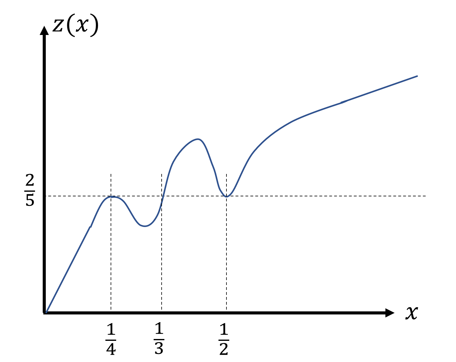
Next, let us apply the bounds in Theorem 4 to an open set and its closure, and see that they do not coincide (in some cases). Consider the sets and . Then we get that the upper bound (80) is equal to , since contains the constant graphon , , which is the global maximum entropy graphon. However, the lower bound (81) must be strictly smaller than , since contains only graphons with . An example with a countable number of jump discontinuities can be constructed in a similar way.
A.2 Proof of Szemerédi’s Regularity Lemma
We prove Szemerédi’s regularity lemma, to make the paper more self-contained for readers less familiar with it. We prove a slightly weaker version of Lemma 1, where the size of the sets in the partition are not necessarily equal sized. Also, we only show that for any , for each graph there exist some such that it has an partition, rather that there is a single that fits all graphs (for large enough). We chose to prove this version, which is based on the one available on Wikipedia, since its proof is short and intuitive; the proof of the full version appearing in Lemma 1 can be found in [2]. The course of the proof will be as follows: for a given graph we first start with some arbitrary partition of size . Then, if this partition is not -uniform we perform a refinement step where each set is partitioned to at most parts. We repeat this step while the partition is not -uniform. We will show that as long as the partition is not -uniform, the refinement step increases the ”energy” of the partition (to be defined later). Since this energy property is bounded from above, this process is finite and bound to produce some -uniform partition.
To that end we need the following lemmas that will show the energy cannot decrease upon refinement, and most increase if the partition to be refined is not -uniform. Let be some graph on vertices and let . Define
For partitions of and of define
Then, for a partition of we define the energy of the partition as
Note that for any since by definition. First we show that the energy is non increasing upon refinement.
Lemma 13.
Let and be some partitions of and respectively, then
| (82) |
Proof.
Let of and , and let us choose a vertex from and a vertex from uniformly at random. Let and be the subsets that and belongs to in the partitions and , respectively, and define the random variable . Then
| (83) |
and
| (84) |
By convexity we have which yields the desired result. ∎
Next, we show that if a pair of sets is not -uniform, there exist a refinement for the pair that will boost its energy.
Lemma 14.
If the pair of sets is not -uniform as witnessed by and , then
| (85) |
Proof.
Define as in the previous lemma. Then
| (86) |
Note that with probability , hence
| (87) |
which concludes the proof. ∎
Lemma 15.
If a partition of is not -uniform, then there exists a refinement of in which every set is partitioned into at most parts and
| (88) |
Proof.
For any such that is not -uniform, find the subsets and that witness the irregularity. Let be the refinement of by all the subsets , . Then, in this partition each set is partitioned into at most parts. Denote by the partitioning of in , then,
Since is a refinement of we get that
| (99) |
where (A.2) is due to Lemma 13, (A.2) is due to Lemma 14, and (99) is since is not -uniform. ∎
Proof of Szemerédi regularity lemma.
We start with a trivial partition () and while the partition is not -uniform we apply Lemma 15. At each step the energy of the partition increases by at least , but , hence we bound to stop, i.e., get an -uniform partition, after at most steps. ∎
A.3 Proof of Fainleib’s inequality
We now bring a sketch of the proof of Fainleib’s inequality (26). The full version including the exact value of the constants can be found in [35].
Proof.
The concept of the proof is to show that there exist a low pass filter such that for any cumulative distribution function it hold that , for some constant . Therefor for any and any two c.d.fs and the expression where the latter is a function that depend on the concentration of . Let be a filter such that for some constants the following properties hold:
- 1.
, for all ;
- 2.
;
- 3.
;
- 4.
, the Fourier transform of is
- •
band limited, , for all ,
- •
bounded, ,
- •
symmetric in absolute value .
- •
Then, since is a c.d.f, i.e. monotonically increasing function, and by letting , we get that indeed
| (100) |
where we used property 3. Then we can write
| (101) | ||||
| (102) | ||||
| (103) | ||||
| (104) |
where in 102 and 104 we used property 2 and in 103 we used property 1. Then, we have
| (105) | ||||
| (106) | ||||
| (107) | ||||
| (108) |
It can be easily shown that there exist a constant such that (full derivation in [35]). Then
| (109) | ||||
| (110) |
When and corresponds to some continuous pdfs and respectively, then the characteristics functions and are their Fourier transforms and we obtain
| (111) | ||||
| (112) |
where in (112) we used the triangle inequality and property 4. When and does not corresponds to continuous pdfs the same result can be obtained using Levy’s inversion, full derivation available at [35]. It is left then to deal with the term . Let , then
| (113) | ||||
| (114) |
Then by combining all three terms together and switching wings we get the desired results. In [35] it is shown that the filter
| (115) |
hold all the required properties. For the exact constants the reader is referred to the full proof there. ∎
A.4 Proof of the Counting Lemma
Proof of Lemma 6.
Here we prove the lemma for the case where is a clique. The proof can be easily amended to account for general graphs. In the following, an irregular pair is a pair of subsets in the -uniform partition that is not an -uniform pair. Also, we denote . Let be a graph that corresponds to an -uniform partition . The reduced graph is obtained from by removing the following edges (recall that ):
- 1.
All edges with at least one end in . There are at most of those.
- 2.
All edges inside the sets . There are at most of those.
- 3.
All edges between irregular pairs . There are at most of those.
- 4.
All edges that belong to -uniform pairs with density . There are at most of those.
Let us upper bound the number of copies of that was removed in the reduction process. There are several cases of such copies:
- 1.
Copies with at least one vertex in . There are at most of those.
- 2.
Copies with at least two vertices in the same set. There are at most of those.
- 3.
Copies with each vertex in a different set but with (at least one) irregular couple. There are at most of those.
- 4.
Copies with each vertex in a different set but with (at least one) less-than- couple. There are at most of those.
Therefore, we have .
Next, note that is a -partite graph on the sets where all the pairs , , in the partition are -uniform with densities
Let us lower bound the number of copies of in . We say that a vertex is typical with respect to , , if it is connected to at least vertices in . If is not typical with respect to then it is atypical with respect to . Note that for any -uniform pair , there are at most vertices in that are atypical with respect to (if there were more, they would form a subset , with size and , in contradiction to being an -uniform pair). Hence, given a specific -let of distinct sets , we have that there are at least vertices in that are typical with respect to all , . Let us look at a specific such vertex . Denote the span of in by , and note that , , and that for any such that we get . Next, note that there are at least vertices in that are typical with respect to all , , thus connected to at least vertices in each , . Let us choose one such vertex, , and repeat the process again. After repeating the process times, we have a subset of vertices {, that are all connected to each other and to the same , vertices in , . We denote these subsets as . Since we get that
hence the pair (,) has at least
| (116) | ||||
| (117) |
edges between them, each edge completes one copy of (with the vertices ). But, there were options to choose the vertices , , and options to choose . Hence, if we let , and denote by the number of copies of over the -let in , we get
| (118) | ||||
| (119) | ||||
| (120) | ||||
| (121) |
where (121) can be derived using the relations , and , . Then,
| (122) | ||||
| (123) |
with . Next note that since we have
| (124) |
and also
| (125) |
where in the last transition we used the fact the , the taylor series of and the relation . Then we get
| (126) |
Note that since is different from only if or if is irregular pair, which only occurs at of the elements in the sum, we get that
Hence, after considering the copies that was lost in the reduction process, we get
| (127) | ||||
| (128) |
where (128) is true for any . The upper bound is derived in a similar way. ∎
A.5 Proof of Lemma 8
To prove this this lemma we first need the following: we say that a bipartite graph if -uniform if are an -uniform pair. In all the following .
Lemma 16.
All bipartite graph with edges over , except for a fraction of at most , are -uniform.
Proof.
Let and be a random bipartite graph with , that is obtained by drawing edges between and independently. Let be the event that is not -uniform, i.e., the event where there exist two subsets , such that , and (denote this event by ) or (denote this event by ). Then, using Hoeffding’s inequality and the union bound
| (129) | ||||
| (130) | ||||
| (131) | ||||
| (132) |
where in (131) we maximized the term using the choice , , and the exponent using the choice . Denote by the set of all bipartite graphs with exactly edges and by the set of all such graphs that are not -uniform. Recall that the distribution is uniform over all the graphs in and that [9]. Then
| (133) | ||||
| (134) | ||||
| (135) |
∎
Proof of Lemma 8.
There are three degrees of freedom in constructing a graph in :
- 1.
Choosing all the edges between -uniform pairs: without the -uniformity constraint, this is equivalent to simply choosing the edges between and , which has options[9]. Using the above claim we can deduce that the -uniformity constraint does not change this number significantly, and we get .
- 2.
Choosing the edges inside the sets: there are at most options.
- 3.
Choosing the edges between irregular pairs: there are at most such pairs, hence options.
Hence we get
| (136) | ||||
| (137) |
∎
References
- [1] I. Csiszár and J. Körner, Information theory: coding theorems for discrete memoryless systems. Orlando, FL, USA: Academic Press, Inc., 1982.
- [2] E. Szemeredi, “Regular partitions of graphs.,” Tech. Rep. STAN-CS-75-489, Stanford, CA, USA, 1975.
- [3] M. Faloutsos, P. Faloutsos, and C. Faloutsos, “On power-law relationships of the internet topology,” ACM SIGCOMM computer communication review, vol. 29, no. 4, pp. 251–262, 1999.
- [4] M. E. Newman, “Random graphs with clustering,” Physical review letters, vol. 103, no. 5, p. 058701, 2009.
- [5] J. C. Miller, “Percolation and epidemics in random clustered networks,” Physical Review E, vol. 80, no. 2, p. 020901, 2009.
- [6] B. Karrer and M. E. Newman, “Random graphs containing arbitrary distributions of subgraphs,” Physical Review E, vol. 82, no. 6, p. 066118, 2010.
- [7] M. Ritchie, L. Berthouze, T. House, and I. Z. Kiss, “Higher-order structure and epidemic dynamics in clustered networks,” Journal of Theoretical Biology, vol. 348, pp. 21–32, 2014.
- [8] M. Ritchie, L. Berthouze, and I. Z. Kiss, “Generation and analysis of networks with a prescribed degree sequence and subgraph family: higher-order structure matters,” Journal of complex networks, vol. 5, no. 1, pp. 1–31, 2017.
- [9] T. M. Cover, Elements of information theory. John Wiley & Sons, 1999.
- [10] T. Schank and D. Wagner, “Finding, counting and listing all triangles in large graphs, an experimental study,” in Experimental and Efficient Algorithms: 4th International Workshop, WEA 2005, Santorini Island, Greece, May 10-13, 2005. Proceedings 4, pp. 606–609, Springer, 2005.
- [11] T. Kloks, D. Kratsch, and H. Müller, “Finding and counting small induced subgraphs efficiently,” Information Processing Letters, vol. 74, no. 3-4, pp. 115–121, 2000.
- [12] S. Chu and J. Cheng, “Triangle listing in massive networks and its applications,” in Proceedings of the 17th ACM SIGKDD international conference on Knowledge discovery and data mining, pp. 672–680, 2011.
- [13] N. Chiba and T. Nishizeki, “Arboricity and subgraph listing algorithms,” SIAM Journal on computing, vol. 14, no. 1, pp. 210–223, 1985.
- [14] L. Becchetti, P. Boldi, C. Castillo, and A. Gionis, “Efficient semi-streaming algorithms for local triangle counting in massive graphs,” in Proceedings of the 14th ACM SIGKDD international conference on Knowledge discovery and data mining, pp. 16–24, 2008.
- [15] L. Becchetti, P. Boldi, C. Castillo, and A. Gionis, “Efficient algorithms for large-scale local triangle counting,” ACM Transactions on Knowledge Discovery from Data (TKDD), vol. 4, no. 3, pp. 1–28, 2010.
- [16] S. Suri and S. Vassilvitskii, “Counting triangles and the curse of the last reducer,” in Proceedings of the 20th international conference on World wide web, pp. 607–614, 2011.
- [17] D. J. Watts and S. H. Strogatz, “Collective dynamics of ‘small-world’networks,” nature, vol. 393, no. 6684, pp. 440–442, 1998.
- [18] R. Albert and A.-L. Barabási, “Statistical mechanics of complex networks,” Reviews of modern physics, vol. 74, no. 1, p. 47, 2002.
- [19] R. Bustin and O. Shayevitz, “On lossy compression of directed graphs,” IEEE Transactions on Information Theory, 2021.
- [20] A. Barvinok, “On the number of matrices and a random matrix with prescribed row and column sums and 0-1 entries,” Advances in Mathematics, vol. 224, pp. 316–339, May 2010.
- [21] A. Barvinok, “Matrices with prescribed row and column sums,” Linear Algebra and its Applications, vol. 436, no. 4, pp. 820–844, 2012.
- [22] S. S. Ioushua and O. Shayevitz, “Counting graphs with a given degree sequence: An information-theoretic perspective,” in 2019 IEEE International Symposium on Information Theory (ISIT), pp. 1492–1496, IEEE, 2019.
- [23] R. Bustin and O. Shayevitz, “On lossy compression of binary matrices,” in Information Theory (ISIT), 2017 IEEE International Symposium on, pp. 1573–1577, IEEE, 2017.
- [24] S. Chatterjee, P. Diaconis, and A. Sly, “Random graphs with a given degree sequence,” The Annals of Applied Probability, vol. 21, no. 4, pp. 1400–1435, 2011.
- [25] H. J. Ryser, “Combinatorial properties of matrices of zeros and ones,” Canad. J. Math, vol. 9, pp. 371–377, 1957.
- [26] D. Gale, “A theorem on flows in networks,” Pacific J. Math, vol. 7, no. 2, pp. 1073–1082, 1957.
- [27] S. Chatterjee and S. S. Varadhan, “The large deviation principle for the Erdős-Rényi random graph,” European Journal of Combinatorics, vol. 32, no. 7, pp. 1000–1017, 2011.
- [28] L. Lovász, Large networks and graph limits, vol. 60. American Mathematical Soc., 2012.
- [29] S. Chatterjee and P. Diaconis, “Estimating and understanding exponential random graph models,” The Annals of Statistics, vol. 41, no. 5, pp. 2428–2461, 2013.
- [30] E. Lubetzky and Y. Zhao, “On replica symmetry of large deviations in random graphs,” Random Structures & Algorithms, vol. 47, no. 1, pp. 109–146, 2015.
- [31] C. Radin and L. Sadun, “Phase transitions in a complex network,” Journal of Physics A: Mathematical and Theoretical, vol. 46, no. 30, p. 305002, 2013.
- [32] R. Kenyon, C. Radin, K. Ren, and L. Sadun, “Multipodal structure and phase transitions in large constrained graphs,” Journal of Statistical Physics, vol. 168, no. 2, pp. 233–258, 2017.
- [33] W. T. Gowers, “Lower bounds of tower type for Szemerédi’s uniformity lemma,” Geometric & Functional Analysis GAFA, vol. 7, no. 2, pp. 322–337, 1997.
- [34] N. Pippenger and M. C. Golumbic, “The inducibility of graphs,” Journal of Combinatorial Theory, Series B, vol. 19, no. 3, pp. 189–203, 1975.
- [35] A. Fainleib, “A generalization of esseen’s inequality and its application in probabilistic number theory,” Izvestiya Rossiiskoi Akademii Nauk. Seriya Matematicheskaya, vol. 32, no. 4, pp. 859–879, 1968.
- [36] C.-G. Esseen, “Fourier analysis of distribution functions. a mathematical study of the laplace-gaussian law,” Acta mathematica, vol. 77, no. 1, pp. 1–125, 1945.
- [37] P. Rigollet and J. Weed, “Uncoupled isotonic regression via minimum wasserstein deconvolution,” Information and Inference: A Journal of the IMA, vol. 8, no. 4, pp. 691–717, 2019.
- [38] R. A. Duke, H. Lefmann, and V. e. c. Rödl, “A fast approximation algorithm for computing the frequencies of subgraphs in a given graph,” SIAM Journal on Computing, vol. 24, no. 3, pp. 598–620, 1995.
- [39] V. Rödl, B. Nagle, J. Skokan, M. Schacht, and Y. Kohayakawa, “The hypergraph regularity method and its applications,” Proceedings of the National Academy of Sciences, vol. 102, no. 23, pp. 8109–8113, 2005.
- [40] V. Rödl and M. Schacht, “Regularity lemmas for graphs,” in Fete of combinatorics and computer science, pp. 287–325, Springer, 2010.