New monotonicity formulas for the curve shortening flow in $\mathbb{R}^{3}$

Hayk Mikayelyan Address: Mathematical Sciences
The University of Nottingham Ningbo China
Taikang Dong Lu Nr. 199, Ningbo 315100
PR China Email address: Hayk.Mikayelyan@nottingham.edu.cn

Date: August 11, 2026

Abstract.

We apply the stabilization technique, developed by T. Zelenyak in 1960s for parabolic equations, on curve shortening flow in $\mathbb{R}^{3}$ , and derive several new monotonicity formulas. All of them share one main feature: the dependence of the “energy” term on the angle between the position vector and the plane orthogonal to the tangent vector. The first formula deals with the projection of the curve on the unit sphere, and computes the derivative of its length. The second formula is the generalization of the classical formula of G. Huisken, while the third one is the generalization of the monotonicity formula with logarithmic terms previously derived by the author for plane curves, [15].

AMS MSC2020: 53E10; 35K40; 35K93

Keywords: curve shortening flow, monotonicity formula

1. Introduction

The curve shortening problem is one of the most beautiful and classical problems in geometric PDEs. It models a curve moving by its curvature vector, and questions like singularity formation, long time asymptotics of rescaled solutions, existence of ancient solutions, etc., have been in the focus of research in past decades. We give a short introduction of the problem in Section 1.1, and would like to refer the reader to the following book and lecture notes [7, 12], as well as some important results [1, 3, 2, 4, 5, 6, 8, 9, 10, 11, 13, 14], for a comprehensive introduction to the topic.

In this article we develop ideas from [15], where a new monotonicity formula has been derived for the curve shortening flow in the plane, to obtain several monotonicity formulas in $\mathbb{R}^{3}$ . The idea is based on techniques from the article by T. Zelenyak [17], where general monotonicity formulas for parabolic problems on an interval have been derived. This allows to compute the time derivative of certain “energies” depending on the angle between the position vector and the plane orthogonal to the tangent vector. In $\mathbb{R}^{2}$ the angle between the position vector and the normal vector has been considered mainly in the context of the support functions of convex curves (see [10], [7]). To the best knowledge of the author, however, monotonicity formulas involving the support functions have not been considered.

Our first monotonicity formula, see Section 2, deals with the projection of the curve on the unit sphere, and computes the derivative of its length. Since this quantity is constant for plane, star-shaped curves (see Corollary 1 on page 1), the right hand side of our formula measures how much a curve in $\mathbb{R}^{3}$ deviates from being plane and “star-shaped”.

Huisken’s monotonicity formula (see [13]) plays a crucial role in the theory of flows driven by the mean curvature, in particular the curve shortening flow (see the equation (9) on page 9). The second formula we derive is the generalization of this classical formula, which is not covered by the larger class of monotonicity formulas introduced in [14], Corollary 4.2.

Our third formula is the generalization of the monotonicity formula with logarithmic terms, previously derived by the author for the star-shaped plane curves, see [15].

The results we present provide more involved tools for the analysis of the stability of the curves, and we believe that the method introduced can be applied for other geometric co-dimension two problems in $\mathbb{R}^{3}$ .

1.1. Problem setting

We consider a closed curve in $\mathbb{R}^{3}$ moving by its curvature

\partial_{t}\gamma=\kappa\nu,

where $\gamma:(0,T)\times S^{1}\to\mathbb{R}^{3}$ is the curve parametrization,

(1)

\kappa=\frac{|\gamma^{\prime\prime}\times\gamma^{\prime}|}{|\gamma^{\prime}|^{3}}

is the curvature and

\nu=\frac{\gamma^{\prime}\times(\gamma^{\prime\prime}\times\gamma^{\prime})}{|\gamma^{\prime}||\gamma^{\prime\prime}\times\gamma^{\prime}|}

is the normal vector. Here ^′ means the derivative in $x\in S^{1}$ variable.

Assume the first singularity appears at point $0$ after finite time $T$ . We rescale the parametrization in the following way

\tau=-\log(T-t),\,\,\,\,\,\,\,\tilde{\gamma}(\tau,x)=(T-t)^{-\frac{1}{2}}\gamma(t,x)

and arrive at

(2)

\partial_{\tau}\tilde{\gamma}=\frac{1}{2}{\tilde{\gamma}}+\frac{{\tilde{\gamma}}^{\prime}\times({\tilde{\gamma}}^{\prime\prime}\times{\tilde{\gamma}}^{\prime})}{|{\tilde{\gamma}}^{\prime}|^{4}},

which is going to be the main equation we consider in this article.

Throughout the paper

\psi=\arcsin\frac{\langle{\tilde{\gamma}},{\tilde{\gamma}}^{\prime}\rangle}{|{\tilde{\gamma}}||{\tilde{\gamma}}^{\prime}|}\in[-\tfrac{\pi}{2},\tfrac{\pi}{2}]

will denote the angle between the position vector ${\tilde{\gamma}}$ and the plane orthogonal to the tangent vector ${\tilde{\gamma}}^{\prime}$ , with a sign coming from the sign of $\langle{\tilde{\gamma}},{\tilde{\gamma}}^{\prime}\rangle$ .

The paper is organized as follows: in Section 2 the main results are introduced, in Section 3 the stabilization technique is presented, and in Section 4 this technique is illustrated on the classical formula of G. Huisken. In Section 5 some “heavy” computations of the so-called remainder terms are conducted, and in Section 6 the proofs of the results are derived from these computations.

Acknowledgments. The author would like to express his gratitude and appreciation to Sigurd Angenent and Gerhard Huisken for valuable feedback.

2. Main results

Let us consider the length of the projection of the curve on the unit sphere given by

\int_{S^{1}}\frac{|{\tilde{\gamma}}^{\prime}|}{|{\tilde{\gamma}}|}\cos\psi dx.

The next theorem establishes a monotonicity relation for this length.

Theorem 1.

Let ${\tilde{\gamma}}$ be the rescaled curve shortening flow in (2). Then

(3)

\frac{d}{d\tau}\int_{S^{1}}\frac{|{\tilde{\gamma}}^{\prime}|}{|{\tilde{\gamma}}|}\cos\psi dx=-\int_{S^{1}}\frac{|{\tilde{\gamma}}^{\prime}|}{|{\tilde{\gamma}}|^{3}\cos^{3}\psi}\kappa^{2}\big|\textup{Proj}_{\nu\times{\tilde{\gamma}}^{\prime}}{\tilde{\gamma}}\big|^{2}dx-2\sum_{\psi(x)=\pm\frac{\pi}{2}}\frac{\kappa(x)}{|\tilde{\gamma}(x)|},

where the second sum is taken over the points where $\psi=\pm\frac{\pi}{2}$ (or ${\tilde{\gamma}}\parallel{\tilde{\gamma}}^{\prime}$ ).
Further, let $a\in C([0,\infty))$ be an arbitrary continuous function on $[0,\infty)$ . Then

(4)

\int_{S^{1}}a(|{\tilde{\gamma}}|)|{\tilde{\gamma}}^{\prime}|\sin\psi dx=0.

Corollary 1.

In the case of the plane curves the monotonicity formula (3) is trivial for the curves satisfying the condition

\psi=\arcsin\frac{\langle{\tilde{\gamma}},{\tilde{\gamma}}^{\prime}\rangle}{|{\tilde{\gamma}}||{\tilde{\gamma}}^{\prime}|}\not=\pm\frac{\pi}{2},

and

\int_{S^{1}}\frac{|{\tilde{\gamma}}^{\prime}|}{|{\tilde{\gamma}}|}\cos\psi dx\equiv 2\pi m,

where $m$ is the winding number. For general plane curves we have

(5)

\frac{d}{d\tau}\int_{S^{1}}\frac{|{\tilde{\gamma}}^{\prime}|}{|{\tilde{\gamma}}|}\cos\psi dx=-2\sum_{\psi(x)=\pm\frac{\pi}{2}}\frac{\kappa(x)}{|\tilde{\gamma}(x)|},

where the curvature $\kappa$ is defined in $\mathbb{R}^{3}$ by (1), thus is non-negative.

Remark 1.

If we let the function $a(r)$ in (4) converge to the Dirac function in $r_{0}$ , we will obtain the simple fact that a closed curve, which intersects the sphere of radius $r_{0}$ in non-tangential fashion, exits the sphere and enters it in the same number of points.

Our second result is the generalization of the classical monotonicity formula of G. Huisken.

Theorem 2.

Let ${\tilde{\gamma}}$ be the rescaled curve shortening flow in (2), $\lambda>0$ , and let

(6)

\psi=\arcsin\frac{\langle{\tilde{\gamma}},{\tilde{\gamma}}^{\prime}\rangle}{|{\tilde{\gamma}}||{\tilde{\gamma}}^{\prime}|}.

Then

(7)

\frac{d}{d\tau}\int_{S^{1}}F_{\lambda}({\tilde{\gamma}},{\tilde{\gamma}}^{\prime})dx=-\int_{S^{1}}\left|\kappa+\frac{1}{2}\langle{\tilde{\gamma}},\nu\rangle\right|^{2}\rho_{\lambda}({\tilde{\gamma}},{\tilde{\gamma}}^{\prime})dx\\ -\int_{S^{1}}\left(\frac{1}{4}+(\lambda-1)\frac{\kappa^{2}}{|{\tilde{\gamma}}|^{2}\cos^{2}\psi}\right)|\textup{Proj}_{\nu\times{\tilde{\gamma}}^{\prime}}{\tilde{\gamma}}|^{2}\rho_{\lambda}({\tilde{\gamma}},{\tilde{\gamma}}^{\prime})dx,

where

F_{\lambda}(\xi,\eta)=a_{\lambda}(|\xi|)|\eta|f_{\lambda}(\psi),\,\,\,\rho_{\lambda}(\xi,\eta)=a_{\lambda}(|\xi|)|\eta|g_{\lambda}(\psi),

a_{\lambda}(r)=e^{-\frac{r^{2}}{4\lambda}}r^{\frac{1-\lambda}{\lambda}},\,\,\,g_{\lambda}(\psi)=\left(\tfrac{1}{\cos\psi}\right)^{\frac{\lambda-1}{\lambda}}

and

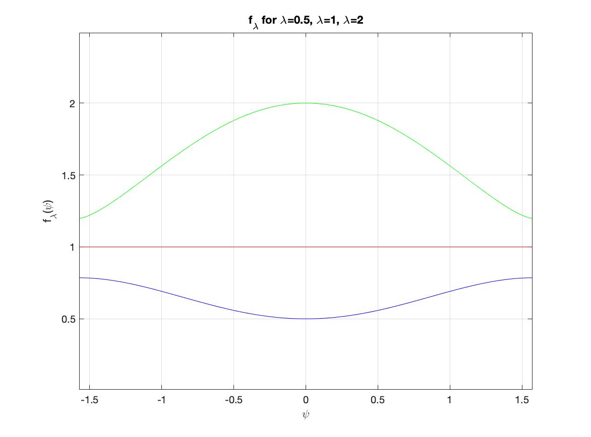
(8)

f_{\lambda}(\psi)=\sin\psi\int_{0}^{\psi}(\cos t)^{\frac{1}{\lambda}}dt+\lambda(\cos\psi)^{1+\frac{1}{\lambda}}.

The graphs of the functions $f_{\lambda}(\psi)$ for several values of $\lambda$ are displayed in Figure 1. Observe that $f_{\lambda}(0)=\lambda$ .

Refer to caption — Figure 1. Functions $f_{\lambda}$ for $\lambda=0.5,\,\,\,1,\text{ and }\,2.$

Remark 2.

For $\lambda=1$ the equation (7) turns into the monotonicity formula of G. Huisken [13] (more details in Section 4)

(9)

\frac{d}{d\tau}\int_{S^{1}}|{\tilde{\gamma}}^{\prime}|e^{-\frac{|{\tilde{\gamma}}|^{2}}{4}}dx=-\int_{S^{1}}\left(\frac{1}{4}|\textup{Proj}_{\nu\times{\tilde{\gamma}}^{\prime}}{\tilde{\gamma}}|^{2}+\left|\kappa+\frac{1}{2}\langle{\tilde{\gamma}},\nu\rangle\right|^{2}\right)|{\tilde{\gamma}}^{\prime}|e^{-\frac{|{\tilde{\gamma}}|^{2}}{4}}dx.

In [15], [16] the version of the following formula has been derived for plane curves, which in $\mathbb{R}^{2}$ happens to be a monotonicity formula. Here we generalize it in $\mathbb{R}^{3}$ .

Theorem 3.

Let ${\tilde{\gamma}}$ be the rescaled curve shortening flow in (2), and let

(10)

\psi=\arcsin\frac{\langle{\tilde{\gamma}},{\tilde{\gamma}}^{\prime}\rangle}{|{\tilde{\gamma}}||{\tilde{\gamma}}^{\prime}|}\not=\pm\frac{\pi}{2}.

Then

(11)

\frac{d}{d\tau}\int_{S^{1}}F({\tilde{\gamma}},{\tilde{\gamma}}^{\prime})dx=-\int_{S^{1}}\left|\kappa+\frac{1}{2}\langle{\tilde{\gamma}},\nu\rangle\right|^{2}\rho({\tilde{\gamma}},{\tilde{\gamma}}^{\prime})dx\\ -\int_{S^{1}}\left[\frac{1}{4}-\Big(1+|{\tilde{\gamma}}|b(|{\tilde{\gamma}}|)-\log\cos\psi\Big)\frac{\kappa^{2}}{|{\tilde{\gamma}}|^{2}\cos^{2}\psi}\right]\big|\textup{Proj}_{\nu\times{\tilde{\gamma}}^{\prime}}{\tilde{\gamma}}\big|^{2}\rho({\tilde{\gamma}},{\tilde{\gamma}}^{\prime})dx,

where

F(\xi,\eta)=\frac{|\eta|}{|\xi|}\Big(h(\psi)-|\xi|b(|\xi|)\cos\psi\Big),\,\,\,\rho(\xi,\eta)=\frac{|\eta|}{|\xi|}\frac{1}{\cos\psi},

h(\psi)=\psi\sin\psi+\cos\psi\log\cos\psi

and

b(r)=\frac{r}{4}-\frac{\log r}{r}-\frac{1-\log 2}{2r}.

The graphs of the functions $f(\psi)$ and $rb(r)$ are displayed in Figure 2.

Remark 3.

Observe that both $h(\psi)$ and $rb(r)$ (see Figure 2) are non-negative convex functions, and achieve their minimum value zero at $\psi=0$ and $r=\sqrt{2}$ respectively, which correspond to the plane circle of radius $\sqrt{2}$ , i.e., the stable stationary plane solution of (2).

Moreover, for the plane circle of radius $\sqrt{2}$ in the second term of (11) not only $\big|\textup{Proj}_{\nu\times{\tilde{\gamma}}^{\prime}}{\tilde{\gamma}}\big|$ vanishes, but also the expression

\left[\frac{1}{4}-\Big(1+|{\tilde{\gamma}}|b(|{\tilde{\gamma}}|)-\log\cos\psi\Big)\frac{\kappa^{2}}{|{\tilde{\gamma}}|^{2}\cos^{2}\psi}\right]

does.

The method of the proof in [15] is interesting because it allows one to derive the monotonicity formula “from nowhere” in $\mathbb{R}^{2}$ . The same approach would fail in $\mathbb{R}^{3}$ , but one can generalize some computations from [15] to $\mathbb{R}^{3}$ for a special class of functions, and obtain new monotonicity formulas. This is what we do in the next two sections.

3. The stabilization technique

For the system (2) we look for functions $F(\xi,\eta)$ and $\rho(\xi,\eta)$ , $\xi,\eta\in\mathbb{R}^{3}$ , to make the following monotonicity relation possible

(12)

\frac{d}{d\tau}\int_{S^{1}}F(v_{1},v_{2},v_{3},v_{1}^{\prime},v_{2}^{\prime},v_{3}^{\prime})dx=-\int_{S^{1}}|\partial_{\tau}\gamma|^{2}\rho(v_{1},v_{2},v_{3},v_{1}^{\prime},v_{2}^{\prime},v_{3}^{\prime})dx+\mathfrak{D}(\tau),

where $\tilde{\gamma}(\tau,x)=\left(\begin{array}[]{cc}v_{1}(\tau,x)\\ v_{2}(\tau,x)\\ v_{3}(\tau,x)\end{array}\right)$ and $\mathfrak{D}$ has a geometric meaning.

Differentiatng the left hand side of (12) and integrating by parts we obtain under the integral

(13)		$\displaystyle\partial_{\tau}v_{1}\left[\frac{\partial F}{\partial\xi_{1}}-\frac{\partial^{2}F}{\partial\xi_{1}\partial\eta_{1}}v_{1}^{\prime}-\frac{\partial^{2}F}{\partial\xi_{2}\partial\eta_{1}}v_{2}^{\prime}-\frac{\partial^{2}F}{\partial\xi_{3}\partial\eta_{1}}v_{3}^{\prime}{\color[rgb]{0,0,1}-\frac{\partial^{2}F}{\partial\eta_{1}^{2}}v_{1}^{\prime\prime}-\frac{\partial^{2}F}{\partial\eta_{1}\partial\eta_{2}}v_{2}^{\prime\prime}-\frac{\partial^{2}F}{\partial\eta_{1}\partial\eta_{3}}v_{3}^{\prime\prime}}\right]\,\,\,$
	$\displaystyle+\partial_{\tau}v_{2}\left[\frac{\partial F}{\partial\xi_{2}}-\frac{\partial^{2}F}{\partial\xi_{1}\partial\eta_{2}}v_{1}^{\prime}-\frac{\partial^{2}F}{\partial\xi_{2}\partial\eta_{2}}v_{2}^{\prime}-\frac{\partial^{2}F}{\partial\xi_{3}\partial\eta_{2}}v_{3}^{\prime}{\color[rgb]{0,0,1}-\frac{\partial^{2}F}{\partial\eta_{1}\partial\eta_{2}}v_{1}^{\prime\prime}-\frac{\partial^{2}F}{\partial\eta_{2}^{2}}v_{2}^{\prime\prime}-\frac{\partial^{2}F}{\partial\eta_{2}\partial\eta_{3}}v_{3}^{\prime\prime}}\right]\,\,\,$
	$\displaystyle+\partial_{\tau}v_{3}\left[\frac{\partial F}{\partial\xi_{3}}-\frac{\partial^{2}F}{\partial\xi_{1}\partial\eta_{3}}v_{1}^{\prime}-\frac{\partial^{2}F}{\partial\xi_{2}\partial\eta_{3}}v_{2}^{\prime}-\frac{\partial^{2}F}{\partial\xi_{3}\partial\eta_{3}}v_{3}^{\prime}{\color[rgb]{0,0,1}-\frac{\partial^{2}F}{\partial\eta_{1}\partial\eta_{3}}v_{1}^{\prime\prime}-\frac{\partial^{2}F}{\partial\eta_{2}\partial\eta_{3}}v_{2}^{\prime\prime}-\frac{\partial^{2}F}{\partial\eta_{3}^{2}}v_{3}^{\prime\prime}}\right].$

In the first entry of the right hand side of (12) using (2) we obtain under the integral

	$\displaystyle\|\partial_{\tau}{\tilde{\gamma}}\|^{2}=\left(\begin{array}[]{cc}\partial_{\tau}v_{1}\\ \partial_{\tau}v_{2}\\ \partial_{\tau}v_{3}\end{array}\right)\left(\frac{1}{2}{\tilde{\gamma}}+\frac{{\tilde{\gamma}}^{\prime}\times({\tilde{\gamma}}^{\prime\prime}\times{\tilde{\gamma}}^{\prime})}{\|{\tilde{\gamma}}^{\prime}\|^{4}}\right)=$
	$\displaystyle\frac{1}{2}\left(\begin{array}[]{cc}\partial_{\tau}v_{1}\\ \partial_{\tau}v_{2}\\ \partial_{\tau}v_{3}\end{array}\right)\cdot{\tilde{\gamma}}+{\color[rgb]{0,0,1}\left(\begin{array}[]{cc}\partial_{\tau}v_{1}\\ \partial_{\tau}v_{2}\\ \partial_{\tau}v_{3}\end{array}\right)\cdot\frac{{\tilde{\gamma}}^{\prime}\times({\tilde{\gamma}}^{\prime\prime}\times{\tilde{\gamma}}^{\prime})}{\|{\tilde{\gamma}}^{\prime}\|^{4}}}.$

Observe that

\frac{{\tilde{\gamma}}^{\prime}\times({\tilde{\gamma}}^{\prime\prime}\times{\tilde{\gamma}}^{\prime})}{|{\tilde{\gamma}}^{\prime}|^{4}}=\frac{1}{|{\tilde{\gamma}}^{\prime}|^{4}}\left(\begin{array}[]{cc}({v^{\prime}}_{2}^{2}+{v^{\prime}}_{3}^{2})v_{1}^{\prime\prime}-v_{1}^{\prime}v_{2}^{\prime}v_{2}^{\prime\prime}-v_{1}^{\prime}v_{3}^{\prime}v_{3}^{\prime\prime}\\ -v_{1}^{\prime}v_{2}^{\prime}v_{1}^{\prime\prime}+({v^{\prime}}_{3}^{2}+{v^{\prime}}_{1}^{2})v_{2}^{\prime\prime}-v_{2}^{\prime}v_{3}^{\prime}v_{3}^{\prime\prime}\\ -v_{1}^{\prime}v_{3}^{\prime}v_{1}^{\prime\prime}-v_{2}^{\prime}v_{3}^{\prime}v_{2}^{\prime\prime}+({v^{\prime}}_{1}^{2}+{v^{\prime}}_{2}^{2})v_{3}^{\prime\prime}\end{array}\right)

and

D^{2}|\eta|=|\eta|^{-3}\left(\begin{array}[]{ccc}(\eta_{2}^{2}+\eta_{3}^{2})&-\eta_{1}\eta_{2}&-\eta_{1}\eta_{3}\\ -\eta_{1}\eta_{2}&(\eta_{1}^{2}+\eta_{3}^{2})&-\eta_{2}\eta_{3}\\ -\eta_{1}\eta_{3}&-\eta_{2}\eta_{3}&(\eta_{1}^{2}+\eta_{2}^{2})\end{array}\right)=|\eta|^{-3}\left(|\eta|^{2}I-(\eta_{i}\eta_{j})_{i,j}\right).

To analyse the terms containing second order derivatives in equations (13) and (3) we will study the action of the matrices

(23)

D^{2}_{\eta}F(\xi,\eta)\,\,\,\text{ and }\,\,\,\rho(\xi,\eta)|\eta|^{-1}D^{2}|\eta|

on the vector ${\tilde{\gamma}}^{\prime\prime}$ . In the case of Huisken’s monotonicity formula the function $F$ depends only on $|\xi|$ , $|\eta|$ and two matrices coincide (see Section 4). In the case of the new monotonicity formulas their difference will have rank one and in Section 5.1 we will show this.

Let us now take

\mathfrak{D}(\tau)=\int_{S^{1}}\mathfrak{D}_{1}+\mathfrak{D}_{2}dx,

where $\mathfrak{D}(\tau)$ is defined by (12), and in $\mathfrak{D}_{2}$ we collect the terms containing ${\tilde{\gamma}}^{\prime\prime}$

(24)

\mathfrak{D}_{2}=\partial_{\tau}{\tilde{\gamma}}\Big[\rho(\xi,\eta)|\eta|^{-1}D^{2}|\eta|-D^{2}_{\eta}F(\xi,\eta)\Big]{\tilde{\gamma}}^{\prime\prime},

and in $\mathfrak{D}_{1}$ the remaining terms

(25)		$\displaystyle\mathfrak{D}_{1}=\partial_{\tau}v_{1}\left[\frac{\partial F}{\partial\xi_{1}}-\frac{\partial^{2}F}{\partial\xi_{1}\partial\eta_{1}}v_{1}^{\prime}-\frac{\partial^{2}F}{\partial\xi_{2}\partial\eta_{1}}v_{2}^{\prime}-\frac{\partial^{2}F}{\partial\xi_{3}\partial\eta_{1}}v_{3}^{\prime}\right]$
	$\displaystyle+\partial_{\tau}v_{2}\left[\frac{\partial F}{\partial\xi_{2}}-\frac{\partial^{2}F}{\partial\xi_{1}\partial\eta_{2}}v_{1}^{\prime}-\frac{\partial^{2}F}{\partial\xi_{2}\partial\eta_{2}}v_{2}^{\prime}-\frac{\partial^{2}F}{\partial\xi_{3}\partial\eta_{2}}v_{3}^{\prime}\right]$
	$\displaystyle+\partial_{\tau}v_{3}\left[\frac{\partial F}{\partial\xi_{3}}-\frac{\partial^{2}F}{\partial\xi_{1}\partial\eta_{3}}v_{1}^{\prime}-\frac{\partial^{2}F}{\partial\xi_{2}\partial\eta_{3}}v_{2}^{\prime}-\frac{\partial^{2}F}{\partial\xi_{3}\partial\eta_{3}}v_{3}^{\prime}\right]$
	$\displaystyle+\rho(\xi,\eta)\left(\begin{array}[]{cc}\partial_{\tau}v_{1}\\ \partial_{\tau}v_{2}\\ \partial_{\tau}v_{3}\end{array}\right)\cdot\frac{1}{2}{\tilde{\gamma}}.$

In Section 5 we will compute $\mathfrak{D}_{1}$ and $\mathfrak{D}_{2}$ for a special class of functions $F$ and $\rho$ and will then derive several new monotonicity formulas in Section 6.

4. Huisken’s monotonicity formula

As an intermediate step let us verify Huisken’s monotonicity formula in our setting. If we take

F(\xi,\eta)=\rho(\xi,\eta)=|\eta|e^{-\frac{|\xi|^{2}}{4}}

then the matrices in (23) will coincide, implying that $\mathfrak{D}_{2}\equiv 0$ .

Further observe that

\displaystyle\left(\begin{array}[]{cc}\frac{\partial F}{\partial\xi_{1}}-\frac{\partial^{2}F}{\partial\xi_{1}\partial\eta_{1}}\eta_{1}-\frac{\partial^{2}F}{\partial\xi_{2}\partial\eta_{1}}\eta_{2}-\frac{\partial^{2}F}{\partial\xi_{3}\partial\eta_{1}}\eta_{3}\\ \frac{\partial F}{\partial\xi_{2}}-\frac{\partial^{2}F}{\partial\xi_{1}\partial\eta_{2}}\eta_{1}-\frac{\partial^{2}F}{\partial\xi_{2}\partial\eta_{2}}\eta_{2}-\frac{\partial^{2}F}{\partial\xi_{3}\partial\eta_{2}}\eta_{3}\\ \frac{\partial F}{\partial\xi_{3}}-\frac{\partial^{2}F}{\partial\xi_{1}\partial\eta_{3}}\eta_{1}-\frac{\partial^{2}F}{\partial\xi_{2}\partial\eta_{3}}\eta_{2}-\frac{\partial^{2}F}{\partial\xi_{3}\partial\eta_{3}}\eta_{3}\end{array}\right)=-\frac{1}{2}|\eta|e^{-\frac{|\xi|^{2}}{4}}\left[\xi-\frac{\langle\xi,\eta\rangle}{|\eta|^{2}}\eta\right],

and thus

	$\displaystyle\mathfrak{D}_{1}=\left(\begin{array}[]{cc}\partial_{\tau}v_{1}\\ \partial_{\tau}v_{2}\\ \partial_{\tau}v_{3}\end{array}\right)\left[\left(\begin{array}[]{cc}\frac{\partial F}{\partial\xi_{1}}-\frac{\partial^{2}F}{\partial\xi_{1}\partial\eta_{1}}\eta_{1}-\frac{\partial^{2}F}{\partial\xi_{2}\partial\eta_{1}}\eta_{2}-\frac{\partial^{2}F}{\partial\xi_{3}\partial\eta_{1}}\eta_{3}\\ \frac{\partial F}{\partial\xi_{2}}-\frac{\partial^{2}F}{\partial\xi_{1}\partial\eta_{2}}\eta_{1}-\frac{\partial^{2}F}{\partial\xi_{2}\partial\eta_{2}}\eta_{2}-\frac{\partial^{2}F}{\partial\xi_{3}\partial\eta_{2}}\eta_{3}\\ \frac{\partial F}{\partial\xi_{3}}-\frac{\partial^{2}F}{\partial\xi_{1}\partial\eta_{3}}\eta_{1}-\frac{\partial^{2}F}{\partial\xi_{2}\partial\eta_{3}}\eta_{2}-\frac{\partial^{2}F}{\partial\xi_{3}\partial\eta_{3}}\eta_{3}\end{array}\right)+\frac{1}{2}\rho(\xi,\eta)\xi\right]$
	$\displaystyle=\rho(\xi,\eta)\left(\frac{1}{2}\xi+\kappa\nu\right)\frac{\langle\xi,\eta\rangle}{2\|\eta\|^{2}}\eta=\frac{\langle\xi,\eta\rangle^{2}}{4\|\eta\|^{2}}\rho(\xi,\eta)=\frac{1}{4}\big\|\textup{Proj}_{\eta}\xi\big\|^{2}\rho(\xi,\eta).$

We have obtained

(38)

\frac{d}{d\tau}\int_{S^{1}}F(v_{1},v_{2},v_{3},v_{1}^{\prime},v_{2}^{\prime},v_{3}^{\prime})dx=-\int_{S^{1}}\left(|\partial_{\tau}{\tilde{\gamma}}|^{2}-\frac{1}{4}\big|\textup{Proj}_{\eta}{\tilde{\gamma}}\big|^{2}\right)\rho(v_{1},v_{2},v_{3},v_{1}^{\prime},v_{2}^{\prime},v_{3}^{\prime})dx.

On the other hand

(39)

\left|\frac{1}{2}\xi+\kappa\nu\right|^{2}-\frac{1}{4}\big|\textup{Proj}_{\eta}\xi\big|^{2}=\\ \frac{1}{4}\left(\big|\textup{Proj}_{\nu}\xi\big|^{2}+\big|\textup{Proj}_{\eta}\xi\big|^{2}+\big|\textup{Proj}_{\nu\times\eta}\xi\big|^{2}\right)+\kappa\langle\xi,\nu\rangle+\kappa^{2}-\frac{1}{4}\big|\textup{Proj}_{\eta}\xi\big|^{2}=\\ \frac{1}{4}\big|\textup{Proj}_{\nu\times\eta}\xi\big|^{2}+\left|\kappa+\frac{1}{2}\langle\xi,\nu\rangle\right|^{2},

implying Huisken’s monotonicity formula (9) for the rescaled curve shortening flow in $\mathbb{R}^{3}$ .

Remark 4.

It has been shown in [15] that using the stabilization technique one can not only verify but actually also re-discover Huisken’s monotonicity formula in $\mathbb{R}^{2}$ .

5. Computations of $\mathfrak{D}$ for a special class of functions $F$ and $\rho$

In the case of the Huisken’s formula functions $F$ and $\rho$ depend only on absolute values of $\xi$ and $\eta$ . Generalizing the approach developed in [15] for plane curves we are looking for formulas, which depend on the angle between $\xi$ and $\eta$ .

Taking into account the matrices (23) we look for the functions $F$ and $\rho$ of the particular form

F(\xi,\eta)=a(|\xi|)|\eta|f(\psi)

and

\rho(\xi,\eta)=a(|\xi|)|\eta|g(\psi),

with

\psi=\arcsin\frac{\langle\xi,\eta\rangle}{|\xi||\eta|}

being the angle between the position vector $\xi=\tilde{\gamma}$ and the plane orthogonal to the tangent $\eta=\tilde{\gamma}^{\prime}$ . The functions $f(\psi)$ , $g(\psi)$ and $a(r)$ will be specified in the upcoming sections.

5.1. Computing $\mathfrak{D}_{2}$

Lemma 1.

f^{\prime\prime}+f=g

then

D^{2}_{\eta}F\,\eta=\rho|\eta|^{-1}D^{2}_{\eta}|\eta|\,\eta=\textbf{0},

(D^{2}_{\eta}F-\rho|\eta|^{-1}D^{2}_{\eta}|\eta|)\,\xi=\textbf{0},

and

(D^{2}_{\eta}F-\rho|\eta|^{-1}D^{2}_{\eta}|\eta|)(\xi\times\eta)=a(|\xi|)\frac{m(\psi)-g(\psi)}{|\eta|}(\xi\times\eta),

where

m(\psi)=f(\psi)-f^{\prime}(\psi)\tan\psi.

Proof.

Let us take

A(\xi,\eta)=|\xi|^{2}|\eta|^{2}-\langle\xi,\eta\rangle^{2}=|\xi|^{2}|\eta|^{2}\cos^{2}\psi,

then

D_{\xi}A=2|\eta|^{2}\xi-2\langle\xi,\eta\rangle\eta,\text{ and }D_{\eta}A=2|\xi|^{2}\eta-2\langle\xi,\eta\rangle\xi,

\langle\eta,D_{\xi}A\rangle=\langle\xi,D_{\eta}A\rangle=0,\text{ and }\langle\xi,D_{\xi}A\rangle=\langle\eta,D_{\eta}A\rangle=2A.

Observe that

\partial_{\eta_{i}}\psi=\frac{|\eta|^{2}\xi_{i}-\langle\xi,\eta\rangle\eta_{i}}{|\eta|^{2}A^{\frac{1}{2}}},\,\,\,\partial_{\xi_{i}}\psi=\frac{|\xi|^{2}\eta_{i}-\langle\xi,\eta\rangle\xi_{i}}{|\xi|^{2}A^{\frac{1}{2}}}.

(40)

\partial^{2}_{\eta_{i}\eta_{j}}\psi=\frac{(2\xi_{i}\eta_{j}-\langle\xi,\eta\rangle\delta_{ij}-\xi_{j}\eta_{i})|\eta|^{2}A^{\frac{1}{2}}}{|\eta|^{4}A}\\ -\frac{(|\eta|^{2}\xi_{i}-\langle\xi,\eta\rangle\eta_{i})(2\eta_{j}A^{\frac{1}{2}}+|\eta|^{2}A^{-\frac{1}{2}}(|\xi|^{2}\eta_{j}-\langle\xi,\eta\rangle\xi_{j}))}{|\eta|^{4}A}\\ =|\eta|^{-4}A^{-1}\Big[-|\eta|^{2}A^{\frac{1}{2}}\langle\xi,\eta\rangle\delta_{ij}+\frac{|\eta|^{4}\langle\xi,\eta\rangle}{A^{\frac{1}{2}}}\xi_{i}\xi_{j}\\ -(\xi_{i}\eta_{j}+\xi_{j}\eta_{i})\frac{|\xi|^{2}|\eta|^{4}}{A^{\frac{1}{2}}}+\frac{2A+|\xi|^{2}|\eta|^{2}}{A^{\frac{1}{2}}}\langle\xi,\eta\rangle\eta_{i}\eta_{j}\Big].

Further

\partial_{\eta_{i}}\left(|\eta|f(\psi)\right)=\partial_{\eta_{i}}|\eta|f(\psi)+|\eta|f^{\prime}(\psi)\partial_{\eta_{i}}\psi

and

(41)

\partial^{2}_{\eta_{i}\eta_{j}}\left(|\eta|f(\psi)\right)=f(\psi)\partial^{2}_{\eta_{i}\eta_{j}}|\eta|\\ +f^{\prime}(\psi)\Big[\partial_{\eta_{j}}|\eta|\partial_{\eta_{i}}\psi+\partial_{\eta_{i}}|\eta|\partial_{\eta_{j}}\psi+|\eta|\partial^{2}_{\eta_{i}\eta_{j}}\psi\Big]\\ +f^{\prime\prime}(\psi)|\eta|\partial_{\eta_{i}}\psi\partial_{\eta_{j}}\psi=

(42)

f(\psi)\partial^{2}_{\eta_{i}\eta_{j}}|\eta|\\ +f^{\prime}(\psi)\Big[-\frac{\langle\xi,\eta\rangle}{|\eta|A^{\frac{1}{2}}}\delta_{ij}+|\eta|\frac{\langle\xi,\eta\rangle}{A^{\frac{3}{2}}}\xi_{i}\xi_{j}-\frac{\langle\xi,\eta\rangle^{2}}{|\eta|A^{\frac{3}{2}}}(\xi_{i}\eta_{j}+\xi_{j}\eta_{i})+\frac{|\xi|^{2}}{|\eta|}\frac{\langle\xi,\eta\rangle}{A^{\frac{3}{2}}}\eta_{i}\eta_{j}\Big]\\ +f^{\prime\prime}(\psi)|\eta|\frac{|\eta|^{4}\xi_{i}\xi_{j}-|\eta|^{2}\langle\xi,\eta\rangle(\xi_{i}\eta_{j}+\xi_{j}\eta_{i})+\langle\xi,\eta\rangle^{2}\eta_{i}\eta_{j}}{|\eta|^{4}A}.

Thus for $\eta$

(43)

D^{2}_{\eta}\left(|\eta|f(\psi)\right)\,\eta=f(\psi)D^{2}_{\eta}|\eta|\,\eta\\ +f^{\prime}(\psi)\Big[-\frac{\langle\xi,\eta\rangle}{|\eta|A^{\frac{1}{2}}}\eta+|\eta|\frac{\langle\xi,\eta\rangle^{2}}{A^{\frac{3}{2}}}\xi-\frac{\langle\xi,\eta\rangle^{2}}{|\eta|A^{\frac{3}{2}}}(|\eta|^{2}\xi+\langle\xi,\eta\rangle\eta)+\frac{|\xi|^{2}}{|\eta|}\frac{\langle\xi,\eta\rangle}{A^{\frac{3}{2}}}|\eta|^{2}\eta\Big]\\ +f^{\prime\prime}(\psi)|\eta|\frac{|\eta|^{4}\langle\xi,\eta\rangle\xi-|\eta|^{2}\langle\xi,\eta\rangle(|\eta|^{2}\xi+\langle\xi,\eta\rangle\eta)+\langle\xi,\eta\rangle^{2}|\eta|^{2}\eta}{|\eta|^{4}A}=\textbf{0}+\textbf{0}+\textbf{0}

since

D^{2}|\eta|\,\eta=|\eta|^{-3}\left(\begin{array}[]{ccc}(\eta_{2}^{2}+\eta_{3}^{2})&-\eta_{1}\eta_{2}&-\eta_{1}\eta_{3}\\ -\eta_{1}\eta_{2}&(\eta_{1}^{2}+\eta_{3}^{2})&-\eta_{2}\eta_{3}\\ -\eta_{1}\eta_{3}&-\eta_{2}\eta_{3}&(\eta_{1}^{2}+\eta_{2}^{2})\end{array}\right)\eta=\textbf{0}.

On the other hand for $\xi$

(44)

D^{2}_{\eta}\left(|\eta|f(\psi)\right)\,\xi=f(\psi)D^{2}_{\eta}|\eta|\,\xi\\ +f^{\prime}(\psi)\Big[-\frac{\langle\xi,\eta\rangle}{|\eta|A^{\frac{1}{2}}}\xi+|\eta||\xi|^{2}\frac{\langle\xi,\eta\rangle}{A^{\frac{3}{2}}}\xi-\frac{\langle\xi,\eta\rangle^{2}}{|\eta|A^{\frac{3}{2}}}(\langle\xi,\eta\rangle\xi+|\xi|^{2}\eta)+\frac{|\xi|^{2}}{|\eta|}\frac{\langle\xi,\eta\rangle^{2}}{A^{\frac{3}{2}}}\eta\Big]\\ +f^{\prime\prime}(\psi)|\eta|\frac{|\eta|^{4}|\xi|^{2}\xi-|\eta|^{2}\langle\xi,\eta\rangle(\langle\xi,\eta\rangle\xi+|\xi|^{2}\eta)+\langle\xi,\eta\rangle^{3}\eta}{|\eta|^{4}A}=

(45)

f(\psi)\frac{1}{|\eta|}\left(\xi-\frac{\langle\xi,\eta\rangle}{|\eta|^{2}}\eta\right)+\textbf{0}+f^{\prime\prime}(\psi)\frac{1}{|\eta|}\left(\xi-\frac{\langle\xi,\eta\rangle}{|\eta|^{2}}\eta\right)=\\ \frac{1}{|\eta|}(f(\psi)+f^{\prime\prime}(\psi))\left(\xi-\frac{\langle\xi,\eta\rangle}{|\eta|^{2}}\eta\right)=|\eta|^{-1}g(\psi)\left(\xi-\frac{\langle\xi,\eta\rangle}{|\eta|^{2}}\eta\right),

while

(46)

D^{2}|\eta|\,\xi=|\eta|^{-3}\left(\begin{array}[]{ccc}(\eta_{2}^{2}+\eta_{3}^{2})&-\eta_{1}\eta_{2}&-\eta_{1}\eta_{3}\\ -\eta_{1}\eta_{2}&(\eta_{1}^{2}+\eta_{3}^{2})&-\eta_{2}\eta_{3}\\ -\eta_{1}\eta_{3}&-\eta_{2}\eta_{3}&(\eta_{1}^{2}+\eta_{2}^{2})\end{array}\right)\xi=\\ \frac{1}{|\eta|^{3}}\left[|\eta|^{2}I-\big(\eta_{i}\eta_{j}\big)_{i,j}\right]\xi=\frac{1}{|\eta|}\left(\xi-\frac{\langle\xi,\eta\rangle}{|\eta|^{2}}\eta\right).

Now let us consider the vector $\xi\times\eta$ . First observe that

D^{2}|\eta|\,(\xi\times\eta)=|\eta|^{-1}(\xi\times\eta).

Then

(47)

D^{2}_{\eta}\left(|\eta|f(\psi)\right)\,(\xi\times\eta)=\left(f(\psi)\frac{1}{|\eta|}-f^{\prime}(\psi)\frac{\langle\xi,\eta\rangle}{|\eta|A^{\frac{1}{2}}}\right)(\xi\times\eta)=\\ \frac{1}{|\eta|}\left(f(\psi)-\tan\psi f^{\prime}(\psi)\right)(\xi\times\eta)=\frac{m(\psi)}{|\eta|}(\xi\times\eta)

and

(D^{2}_{\eta}F-\rho|\eta|^{-1}D^{2}_{\eta}|\eta|)(\xi\times\eta)=a(|\xi|)|\eta|^{-1}\left(m(\psi)-g(\psi)\right)(\xi\times\eta).

∎

Lemma 1 shows that the matrices in (23) do not coincide but it allows one to compute the following difference with $\mu=(v_{1}^{\prime\prime},v_{2}^{\prime\prime},v_{3}^{\prime\prime})^{T}$ :

\left(D^{2}_{\eta}F(\xi,\eta)-\rho(\xi,\eta)|\eta|^{-1}D^{2}|\eta|\right)\mu=\\ \frac{a(|\xi|)}{|\eta|}\left(m(\psi)-g(\psi)\right)\textup{Proj}_{\xi\times\eta}\mu.

Substituting

(48)

\left(\begin{array}[]{cc}\partial_{\tau}v_{1}\\ \partial_{\tau}v_{2}\\ \partial_{\tau}v_{3}\end{array}\right)=\frac{1}{2}{\tilde{\gamma}}+\frac{{\tilde{\gamma}}^{\prime}\times({\tilde{\gamma}}^{\prime\prime}\times{\tilde{\gamma}}^{\prime})}{|{\tilde{\gamma}}^{\prime}|^{4}}=\frac{1}{2}\xi+\frac{\eta\times(\mu\times\eta)}{|\eta|^{4}},

we arrive at

(49)

\partial_{\tau}{\tilde{\gamma}}\left(D^{2}_{\eta}F(\xi,\eta)-\rho(\xi,\eta)|\eta|^{-1}D^{2}|\eta|\right){\tilde{\gamma}}^{\prime\prime}=\\ \frac{a(|\xi|)}{|\eta|}\left(m(\psi)-g(\psi)\right)\left(\frac{1}{2}\xi+\frac{\eta\times(\mu\times\eta)}{|\eta|^{4}}\right)\cdot\textup{Proj}_{\xi\times\eta}\mu.

Observe that

\eta\times(\mu\times\eta)=|\eta|^{2}\mu-\langle\mu,\eta\rangle\eta,

and thus

(50)

\left(\frac{1}{2}\xi+\frac{\eta\times(\mu\times\eta)}{|\eta|^{4}}\right)\cdot\textup{Proj}_{\xi\times\eta}\mu=|\eta|^{-2}\mu\cdot\frac{(\xi\times\eta)\mu}{|(\xi\times\eta)|^{2}}(\xi\times\eta)=\\ \frac{\text{Vol}(\xi,\eta,\mu)^{2}}{|\xi|^{2}|\eta|^{4}\cos^{2}\psi}=\frac{(\xi\cdot(\eta\times\mu))^{2}}{|\xi|^{2}|\eta|^{4}\cos^{2}\psi}=\frac{\kappa^{2}|\eta|^{2}}{|\xi|^{2}\cos^{2}\psi}\left|\textup{Proj}_{\eta\times\nu}\xi\right|^{2},

where $\text{Vol}(\xi,\eta,\mu)=|(\xi\times\eta)\cdot\mu|=|\xi\cdot(\eta\times\mu)|$ is the volume of the parallelepiped formed by vectors $\xi,\eta,\mu$ , and $\kappa=\frac{|\eta\times\mu|}{|\eta|^{3}}$ is the curvature. In the last equality we have used that

\textup{Proj}_{\eta\times\mu}\xi=\textup{Proj}_{\eta\times\nu}\xi.

We have proven the following lemma.

Lemma 2.

Let $\mathfrak{D}_{2}$ be the expression defined in (24), and $f$ , $g$ and $m$ be as in Lemma 1. Then

(51)

\mathfrak{D}_{2}=\partial_{\tau}{\tilde{\gamma}}\left(\rho(\xi,\eta)|\eta|^{-1}D^{2}|\eta|-D^{2}_{\eta}F(\xi,\eta)\right){\tilde{\gamma}}^{\prime\prime}=\\ -a(|{\tilde{\gamma}}|)|{\tilde{\gamma}}^{\prime}|\left(m(\psi)-g(\psi)\right)\frac{\kappa^{2}}{|{\tilde{\gamma}}|^{2}\cos^{2}\psi}\left|\textup{Proj}_{{\tilde{\gamma}}^{\prime}\times\nu}{\tilde{\gamma}}\right|^{2}.

5.2. Computing $\mathfrak{D}_{1}$

Now let us try to compute the difference of the terms which do not contain the second derivatives of ${\tilde{\gamma}}$ :

	$\displaystyle\mathfrak{D}_{1}=\frac{\rho(\xi,\eta)}{2}\left(\begin{array}[]{cc}\partial_{\tau}v_{1}\\ \partial_{\tau}v_{2}\\ \partial_{\tau}v_{3}\end{array}\right)\cdot{\tilde{\gamma}}\,\,\,$
	$\displaystyle+\partial_{\tau}v_{1}\left[\frac{\partial F}{\partial\xi_{1}}-\frac{\partial^{2}F}{\partial\xi_{1}\partial\eta_{1}}v_{1}^{\prime}-\frac{\partial^{2}F}{\partial\xi_{2}\partial\eta_{1}}v_{2}^{\prime}-\frac{\partial^{2}F}{\partial\xi_{3}\partial\eta_{1}}v_{3}^{\prime}\right]\,\,\,$
	$\displaystyle+\partial_{\tau}v_{2}\left[\frac{\partial F}{\partial\xi_{2}}-\frac{\partial^{2}F}{\partial\xi_{1}\partial\eta_{2}}v_{1}^{\prime}-\frac{\partial^{2}F}{\partial\xi_{2}\partial\eta_{2}}v_{2}^{\prime}-\frac{\partial^{2}F}{\partial\xi_{3}\partial\eta_{2}}v_{3}^{\prime}\right]\,\,\,$
	$\displaystyle+\partial_{\tau}v_{3}\left[\frac{\partial F}{\partial\xi_{3}}-\frac{\partial^{2}F}{\partial\xi_{1}\partial\eta_{3}}v_{1}^{\prime}-\frac{\partial^{2}F}{\partial\xi_{2}\partial\eta_{3}}v_{2}^{\prime}-\frac{\partial^{2}F}{\partial\xi_{3}\partial\eta_{3}}v_{3}^{\prime}\right].$

Let us compute

\partial_{\xi_{i}}F-\eta D_{\xi}\left(\frac{\partial F}{\partial\eta_{i}}\right)=\frac{\partial F}{\partial\xi_{i}}-\frac{\partial^{2}F}{\partial\xi_{1}\partial\eta_{i}}\eta_{1}-\frac{\partial^{2}F}{\partial\xi_{2}\partial\eta_{i}}\eta_{2}-\frac{\partial^{2}F}{\partial\xi_{3}\partial\eta_{i}}\eta_{3}

for

F(\xi,\eta)=a(|\xi|)|\eta|f(\psi).

Substituting

\partial_{\xi_{i}}\psi=\frac{1}{\cos\psi}\frac{\eta_{i}}{|\xi||\eta|}-\tan\psi\frac{\xi_{i}}{|\xi|^{2}}\text{ and }\partial_{\eta_{i}}\psi=\frac{1}{\cos\psi}\frac{\xi_{i}}{|\xi||\eta|}-\tan\psi\frac{\eta_{i}}{|\eta|^{2}},

we obtain

(52)

\frac{\partial F}{\partial\xi_{i}}=\frac{|\eta|}{|\xi|}a^{\prime}(|\xi|)f(\psi)\xi_{i}+|\eta|a(|\xi|)f(\psi)\partial_{\xi_{i}}\psi=\\ \frac{|\eta|}{|\xi|}\left(a^{\prime}(|\xi|)f(\psi)-\frac{a(|\xi|)}{|\xi|}f^{\prime}(\psi)\tan\psi\right)\xi_{i}+\frac{a(|\xi|)}{|\xi|}\frac{f^{\prime}(\psi)}{\cos\psi}\eta_{i},

and

(53)

\frac{\partial^{2}F}{\partial\xi_{i}\partial\eta_{j}}=\frac{1}{|\xi||\eta|}\left(a^{\prime}(|\xi|)f(\psi)-\frac{a(|\xi|)}{|\xi|}f^{\prime}(\psi)\tan\psi\right)\xi_{i}\eta_{j}\\ +\frac{|\eta|}{|\xi|}\left(a^{\prime}(|\xi|)f^{\prime}(\psi)-\frac{a(|\xi|)}{|\xi|}(f^{\prime}(\psi)\tan\psi)^{\prime}\right)\xi_{i}\partial_{\eta_{j}}\psi\\ +\frac{a(|\xi|)}{|\xi|}\frac{f^{\prime}(\psi)}{\cos\psi}\delta_{ij}+\frac{a(|\xi|)}{|\xi|}\left(\frac{f^{\prime}(\psi)}{\cos\psi}\right)^{\prime}\eta_{i}\partial_{\eta_{j}}\psi,

and

(54)

\eta D_{\xi}\left(\frac{\partial F}{\partial\eta_{j}}\right)=\frac{1}{|\xi||\eta|}\left(a^{\prime}(|\xi|)f(\psi)-\frac{a(|\xi|)}{|\xi|}f^{\prime}(\psi)\tan\psi\right)\langle\xi,\eta\rangle\eta_{j}\\ +\frac{|\eta|}{|\xi|}\left(a^{\prime}(|\xi|)f^{\prime}(\psi)-\frac{a(|\xi|)}{|\xi|}(f^{\prime}(\psi)\tan\psi)^{\prime}\right)\langle\xi,\eta\rangle\partial_{\eta_{j}}\psi\\ +\frac{a(|\xi|)}{|\xi|}\frac{f^{\prime}(\psi)}{\cos\psi}\eta_{j}+\frac{a(|\xi|)}{|\xi|}\left(\frac{f^{\prime}(\psi)}{\cos\psi}\right)^{\prime}|\eta|^{2}\partial_{\eta_{j}}\psi=\\ \left(a^{\prime}(|\xi|)f(\psi)\sin\psi-\frac{a(|\xi|)}{|\xi|}f^{\prime}(\psi)\tan\psi\sin\psi+\frac{a(|\xi|)}{|\xi|}\frac{f^{\prime}(\psi)}{\cos\psi}\right)\eta_{j}\\ +|\eta|^{2}\left(a^{\prime}(|\xi|)f^{\prime}(\psi)\sin\psi-\frac{a(|\xi|)}{|\xi|}(f^{\prime}(\psi)\tan\psi)^{\prime}\sin\psi+\frac{a(|\xi|)}{|\xi|}\left(\frac{f^{\prime}(\psi)}{\cos\psi}\right)^{\prime}\right)\partial_{\eta_{j}}\psi.

Further

(55)

\partial_{\xi_{i}}F-\eta D_{\xi}\left(\frac{\partial F}{\partial\eta_{i}}\right)=\\ \frac{|\eta|}{|\xi|}\left(a^{\prime}(|\xi|)f(\psi)-\frac{a(|\xi|)}{|\xi|}f^{\prime}(\psi)\tan\psi\right)\xi_{i}+\frac{a(|\xi|)}{|\xi|}\frac{f^{\prime}(\psi)}{\cos\psi}\eta_{i}\\ -\left(a^{\prime}(|\xi|)f(\psi)\sin\psi-\frac{a(|\xi|)}{|\xi|}f^{\prime}(\psi)\tan\psi\sin\psi+\frac{a(|\xi|)}{|\xi|}\frac{f^{\prime}(\psi)}{\cos\psi}\right)\eta_{j}\\ -|\eta|^{2}\left(a^{\prime}(|\xi|)f^{\prime}(\psi)\sin\psi-\frac{a(|\xi|)}{|\xi|}(f^{\prime}(\psi)\tan\psi)^{\prime}\sin\psi+\frac{a(|\xi|)}{|\xi|}\left(\frac{f^{\prime}(\psi)}{\cos\psi}\right)^{\prime}\right)\partial_{\eta_{j}}\psi=

(56)

=\frac{|\eta|}{|\xi|}\Bigg(a^{\prime}(|\xi|)f(\psi)-\frac{a(|\xi|)}{|\xi|}f^{\prime}(\psi)\tan\psi-a^{\prime}(|\xi|)f^{\prime}(\psi)\tan\psi\\ +\frac{a(|\xi|)}{|\xi|}(f^{\prime}(\psi)\tan\psi)^{\prime}\tan\psi-\frac{a(|\xi|)}{|\xi|}\frac{1}{\cos\psi}\left(\frac{f^{\prime}(\psi)}{\cos\psi}\right)^{\prime}\Bigg)\xi_{i}\\ -\Bigg(a^{\prime}(|\xi|)f(\psi)\sin\psi-\frac{a(|\xi|)}{|\xi|}f^{\prime}(\psi)\tan\psi\sin\psi+\frac{a(|\xi|)}{|\xi|}\frac{f^{\prime}(\psi)}{\cos\psi}-\frac{a(|\xi|)}{|\xi|}\frac{f^{\prime}(\psi)}{\cos\psi}\\ -\tan\psi\left[a^{\prime}(|\xi|)f^{\prime}(\psi)\sin\psi-\frac{a(|\xi|)}{|\xi|}(f^{\prime}(\psi)\tan\psi)^{\prime}\sin\psi+\frac{a(|\xi|)}{|\xi|}\left(\frac{f^{\prime}(\psi)}{\cos\psi}\right)^{\prime}\right]\Bigg)\eta_{i},

and observing that

\left(\frac{f^{\prime}(\psi)}{\cos\psi}\right)^{\prime}-(f^{\prime}(\psi)\tan\psi)^{\prime}\sin\psi=f^{\prime\prime}(\psi)\cos\psi,

we arrive at

(57)

\partial_{\xi_{i}}F-\eta D_{\xi}\left(\frac{\partial F}{\partial\eta_{i}}\right)=\\ \left[a^{\prime}(|\xi|)f(\psi)-\left(a^{\prime}(|\xi|)+\frac{a(|\xi|)}{|\xi|}\right)\tan\psi f^{\prime}(\psi)-\frac{a(|\xi|)}{|\xi|}f^{\prime\prime}(\psi)\right]\left(\frac{|\eta|}{|\xi|}\xi_{i}-\sin\psi\eta_{i}\right)=\\ \left[\left(a^{\prime}(|\xi|)+\frac{a(|\xi|)}{|\xi|}\right)(f(\psi)-\tan\psi f^{\prime}(\psi))-\frac{a(|\xi|)}{|\xi|}g(\psi)\right]\left(\frac{|\eta|}{|\xi|}\xi_{i}-\sin\psi\eta_{i}\right)=\\ \left[\left(a^{\prime}(|\xi|)+\frac{a(|\xi|)}{|\xi|}\right)m(\psi)-\frac{a(|\xi|)}{|\xi|}g(\psi)\right]\left(\frac{|\eta|}{|\xi|}\xi_{i}-\sin\psi\eta_{i}\right)=\\ a(|\xi|)|\eta|\left[\frac{1}{|\xi|}\left(\frac{a^{\prime}(|\xi|)}{a(\xi)}+\frac{1}{|\xi|}\right)m(\psi)-\frac{1}{|\xi|^{2}}g(\psi)\right]\left(\xi_{i}-\frac{|\xi|}{|\eta|}\sin\psi\eta_{i}\right).

We have proven the following lemma.

Lemma 3.

Let $\mathfrak{D}_{1}$ be the expression defined in (25), and $f$ , $g$ and $m$ be as in Lemma 1. Then

(58)

\mathfrak{D}_{1}=a(|\xi|)|\eta|\left[\frac{1}{|\xi|}\left(\frac{a^{\prime}(|\xi|)}{a(|\xi|)}+\frac{1}{|\xi|}\right)m(\psi)+\left(\frac{1}{2}-\frac{1}{|\xi|^{2}}\right)g(\psi)\right]\xi\cdot\partial_{\tau}{\tilde{\gamma}}\\ -a(|\xi|)|\xi|\left[\frac{1}{|\xi|}\left(\frac{a^{\prime}(|\xi|)}{a(|\xi|)}+\frac{1}{|\xi|}\right)m(\psi)-\frac{1}{|\xi|^{2}}g(\psi)\right]\sin\psi\,\eta\cdot\partial_{\tau}{\tilde{\gamma}},

where $\xi=\tilde{\gamma}$ and $\eta=\tilde{\gamma}^{\prime}$ .

6. New monotonicity formulas

6.1. Proof of the Theorem 1

Proof.

Let us first observe that (4) follows from (58) and (51) with $f(\psi)=\sin\psi$ resulting

\frac{d}{d\tau}\int_{S^{1}}a(|{\tilde{\gamma}}|)|{\tilde{\gamma}}^{\prime}|\sin\psi dx=0

implies that the integral in (4) must be a constant. This constant is zero because of the known results about convergence to Abresch-Langer curves or a Grim Reaper and their symmetry.

But the equation (4) is rather simple (almost trivial) and can be proven directly. Observe that the expression

\int_{x_{1}}^{x_{2}}|{\tilde{\gamma}}^{\prime}|\sin\psi dx

measures the change of the distance of the point ${\tilde{\gamma}}(\tau,x)$ from the origin, as the parameter $x$ varies from $x_{1}$ to $x_{2}$ . This makes the proof trivial for an arbitrary closed curve ${\tilde{\gamma}}$ and a step-function $a(r)$ . The proof follows now by approximation.

The proof of (3) satisfying the condition (10) follows from (58) and (51) with

f(\psi)=\cos\psi,\,\,\,a(r)=r^{-1}.

For the simplicity let us first consider the case of the plane curves and prove the equation (5) from the Corollary 1.

Since the formula (3) in $\mathbb{R}^{3}$ is correct with respect to any reference point we will write it for the plane curve with respect to the point $(0,0,\epsilon)$ and pass to limit $\epsilon\searrow 0+$ (see Figure 3). Obviously the condition (10) is satisfied if we take $(0,0,\epsilon)$ as the reference point. We have

(59)

\frac{d}{d\tau}\int_{S^{1}}\frac{|{\tilde{\gamma}}_{\epsilon}^{\prime}|}{|{\tilde{\gamma}}_{\epsilon}|}\cos\psi dx=\int_{S^{1}}\frac{|{\tilde{\gamma}}_{\epsilon}^{\prime}|}{|{\tilde{\gamma}}_{\epsilon}|^{3}\cos^{3}\psi}\kappa^{2}|\textup{Proj}_{\nu\times{\tilde{\gamma}}_{\epsilon}^{\prime}}{\tilde{\gamma}}_{\epsilon}|^{2}dx=\\ \int_{\cos\psi<\delta}\frac{|{\tilde{\gamma}}_{\epsilon}^{\prime}|}{|{\tilde{\gamma}}_{\epsilon}|^{3}\cos^{3}\psi}\kappa^{2}|\textup{Proj}_{\nu\times{\tilde{\gamma}}_{\epsilon}^{\prime}}{\tilde{\gamma}}_{\epsilon}|^{2}dx+\int_{\cos\psi\geq\delta}\frac{|{\tilde{\gamma}}_{\epsilon}^{\prime}|}{|{\tilde{\gamma}}_{\epsilon}|^{3}\cos^{3}\psi}\kappa^{2}|\textup{Proj}_{\nu\times{\tilde{\gamma}}_{\epsilon}^{\prime}}{\tilde{\gamma}}_{\epsilon}|^{2}dx\\ =I_{1}+I_{2}.

First let us observe that for arbitrary fixed $\delta>0$

|I_{2}|\leq\delta^{-3}\int_{S_{1}}\frac{\kappa^{2}}{|{\tilde{\gamma}}_{\epsilon}|}\left|\textup{Proj}_{\nu\times{\tilde{\gamma}}_{\epsilon}^{\prime}}\frac{{\tilde{\gamma}}_{\epsilon}}{|{\tilde{\gamma}}_{\epsilon}|}\right|^{2}|{\tilde{\gamma}}_{\epsilon}^{\prime}|dx\to 0.

Let us now choose $\delta>0$ small enough, such that

\{x\in S_{1}\,|\,\cos\psi<\delta\}=\cup_{j\in J}(x_{j}-\omega_{j},x_{j}+\omega_{j}),

where $\cos\psi(x_{j})=0$ and the intervals $(x_{j}-\omega_{j},x_{j}+\omega_{j})$ are disjoint. Let us pick one of these intervals, which we without loss of generality assume to be $(-\omega,\omega)$ . We will compute the limit $\epsilon\to 0$ of the following integral

(60)

\int_{-\omega}^{\omega}\frac{|{\tilde{\gamma}}_{\epsilon}^{\prime}|}{|{\tilde{\gamma}}_{\epsilon}|^{3}\cos^{3}\psi}\kappa^{2}|\textup{Proj}_{\nu\times{\tilde{\gamma}}_{\epsilon}^{\prime}}{\tilde{\gamma}}_{\epsilon}|^{2}dx=\\ \int_{-\omega}^{\omega}\frac{|{\tilde{\gamma}}^{\prime}_{\epsilon}|^{4}}{(|{\tilde{\gamma}}_{\epsilon}|^{2}|{\tilde{\gamma}}^{\prime}_{\epsilon}|^{2}-\langle{\tilde{\gamma}}_{\epsilon},{\tilde{\gamma}}^{\prime}_{\epsilon}\rangle^{2})^{\frac{3}{2}}}\left(\frac{|{\tilde{\gamma}}^{\prime}_{\epsilon}\times{\tilde{\gamma}}^{\prime\prime}_{\epsilon}|}{|{\tilde{\gamma}}^{\prime}_{\epsilon}|^{3}}\right)^{2}|\textup{Proj}_{\nu\times{\tilde{\gamma}}_{\epsilon}^{\prime}}{\tilde{\gamma}}_{\epsilon}|^{2}dx=\\ \int_{-\omega}^{\omega}\frac{1}{(|{\tilde{\gamma}}_{\epsilon}|^{2}|{\tilde{\gamma}}^{\prime}_{\epsilon}|^{2}-\langle{\tilde{\gamma}}_{\epsilon},{\tilde{\gamma}}^{\prime}_{\epsilon}\rangle^{2})^{\frac{3}{2}}}\frac{|{\tilde{\gamma}}^{\prime}_{\epsilon}\times{\tilde{\gamma}}^{\prime\prime}_{\epsilon}|^{2}}{|{\tilde{\gamma}}^{\prime}_{\epsilon}|^{2}}|\textup{Proj}_{\nu\times{\tilde{\gamma}}_{\epsilon}^{\prime}}{\tilde{\gamma}}_{\epsilon}|^{2}dx.

In order to compute this limit we approximate the curve (after rotation) in the interval $x\in(-\omega,\omega)$ by the parabola

(61)

{\tilde{\gamma}}_{\epsilon}(x)=\big(|{\tilde{\gamma}}(0)|+x,\tfrac{1}{2}\kappa(0)x^{2},-\epsilon\big)+(0,O(x^{3}),0),

with

{\tilde{\gamma}}^{\prime}_{\epsilon}(x)=(1,\kappa(0)x,0)+(0,O(x^{2}),0)\,\,\,\text{ and }\,\,\,\,{\tilde{\gamma}}^{\prime\prime}_{\epsilon}(x)=(0,\kappa(0),0)+(0,O(x),0),

and arrive at

(62)

\int_{-\omega}^{\omega}\frac{1}{(|{\tilde{\gamma}}_{\epsilon}|^{2}|{\tilde{\gamma}}^{\prime}_{\epsilon}|^{2}-\langle{\tilde{\gamma}}_{\epsilon},{\tilde{\gamma}}^{\prime}_{\epsilon}\rangle^{2})^{\frac{3}{2}}}\frac{|{\tilde{\gamma}}^{\prime}_{\epsilon}\times{\tilde{\gamma}}^{\prime\prime}_{\epsilon}|^{2}}{|{\tilde{\gamma}}^{\prime}_{\epsilon}|^{2}}|\textup{Proj}_{\nu\times{\tilde{\gamma}}_{\epsilon}^{\prime}}{\tilde{\gamma}}_{\epsilon}|^{2}dx\approx\\ \int_{-\omega}^{\omega}\frac{1}{(\epsilon^{2}(1+\kappa^{2}x^{2})+\kappa^{2}x^{2}(\frac{x}{2}+|{\tilde{\gamma}}|)^{2})^{\frac{3}{2}}}\frac{\kappa^{2}}{(1+\kappa^{2}x^{2})}\epsilon^{2}dx=\\ \frac{\kappa}{|{\tilde{\gamma}}|}\int_{-\omega}^{\omega}\frac{1}{\left((1+\kappa^{2}x^{2})+\frac{\kappa^{2}|{\tilde{\gamma}}|^{2}x^{2}}{\epsilon^{2}}(\frac{x}{2|{\tilde{\gamma}}|}+1)^{2}\right)^{\frac{3}{2}}}\frac{1}{(1+\kappa^{2}x^{2})}d\underbrace{\frac{\kappa|{\tilde{\gamma}}|x}{\epsilon}}_{=\sigma}=\\ \frac{\kappa}{|{\tilde{\gamma}}|}\int_{-\tfrac{\kappa|{\tilde{\gamma}}|\omega}{\epsilon}}^{\tfrac{\kappa|{\tilde{\gamma}}|\omega}{\epsilon}}\frac{1}{(1+\frac{\epsilon^{2}\sigma^{2}}{|{\tilde{\gamma}}|^{2}})\left((1+\frac{\epsilon^{2}\sigma^{2}}{|{\tilde{\gamma}}|^{2}})+\sigma^{2}(\frac{\epsilon\sigma}{2|{\tilde{\gamma}}|^{2}\kappa}+1)^{2}\right)^{\frac{3}{2}}}d\sigma\to_{\epsilon\to 0}\\ \frac{\kappa}{|{\tilde{\gamma}}|}\int_{-\infty}^{\infty}\frac{1}{(1+\sigma^{2})^{\frac{3}{2}}}d\sigma=2\frac{\kappa}{|{\tilde{\gamma}}|},

where starting line two we write $\kappa$ for $\kappa(0)$ and $|{\tilde{\gamma}}|$ for $|{\tilde{\gamma}}(0)|$ , as well as use

\int_{-\infty}^{\infty}\frac{1}{(1+\sigma^{2})^{\frac{3}{2}}}d\sigma=\int_{-\infty}^{\infty}\frac{1}{(\cosh t)^{2}}dt=2.

What remains to observe is that replacing the curve by the parabola in the second line of (62) was justified:

(63)

\bigg|\int_{-\omega}^{\omega}\frac{1}{(|{\tilde{\gamma}}_{\epsilon}|^{2}|{\tilde{\gamma}}^{\prime}_{\epsilon}|^{2}-\langle{\tilde{\gamma}}_{\epsilon},{\tilde{\gamma}}^{\prime}_{\epsilon}\rangle^{2})^{\frac{3}{2}}}\frac{|{\tilde{\gamma}}^{\prime}_{\epsilon}\times{\tilde{\gamma}}^{\prime\prime}_{\epsilon}|^{2}}{|{\tilde{\gamma}}^{\prime}_{\epsilon}|^{2}}|\textup{Proj}_{\nu\times{\tilde{\gamma}}_{\epsilon}^{\prime}}{\tilde{\gamma}}_{\epsilon}|^{2}dx-\\ \int_{-\omega}^{\omega}\frac{1}{(\epsilon^{2}(1+\kappa^{2}x^{2})+\kappa^{2}x^{2}(\frac{x}{2}+|{\tilde{\gamma}}|)^{2})^{\frac{3}{2}}}\frac{\kappa^{2}}{(1+\kappa^{2}x^{2})}\epsilon^{2}dx\bigg|=\\ \bigg|\int_{-\omega}^{\omega}\frac{1}{(\epsilon^{2}(1+\kappa^{2}x^{2})+\kappa^{2}x^{2}(\frac{x}{2}+|{\tilde{\gamma}}|)^{2}+O(x^{3}))^{\frac{3}{2}}}\frac{(\kappa+O(x))^{2}}{(1+\kappa^{2}x^{2}+O(x^{3}))}\epsilon^{2}dx-\\ \int_{-\omega}^{\omega}\frac{1}{(\epsilon^{2}(1+\kappa^{2}x^{2})+\kappa^{2}x^{2}(\frac{x}{2}+|{\tilde{\gamma}}|)^{2})^{\frac{3}{2}}}\frac{\kappa^{2}}{(1+\kappa^{2}x^{2})}\epsilon^{2}dx\bigg|=\\ \bigg|\int_{-\omega}^{\omega}\frac{1}{(\epsilon^{2}(1+\kappa^{2}x^{2})+\kappa^{2}x^{2}(\frac{x}{2}+|{\tilde{\gamma}}|)^{2})^{\frac{3}{2}}}\frac{O(x)}{(1+\kappa^{2}x^{2})}\epsilon^{2}dx\bigg|\leq\\ M\epsilon\int_{-\infty}^{\infty}\frac{|\sigma|}{(1+\sigma^{2})^{\frac{3}{2}}}d\sigma\to_{\epsilon\to 0}0,

where the last inequality follows from the computations in (62), with $M$ being a large enough constant depending on $\tilde{\gamma}$ .

The proof the equation (3) in $\mathbb{R}^{3}$ follows by the same argument. One needs only to observe that if we replace the parabola (61) by the non-plane curve

{\tilde{\gamma}}_{\epsilon}(x)=\big(|{\tilde{\gamma}}(0)|+x,\tfrac{1}{2}\kappa(0)x^{2},-\epsilon\big)+(0,O(x^{3}),O(x^{3})),

then in the computations (63) instead of $|\textup{Proj}_{\nu\times{\tilde{\gamma}}_{\epsilon}^{\prime}}{\tilde{\gamma}}_{\epsilon}|^{2}=\epsilon^{2}$ we will have

|\textup{Proj}_{\nu\times{\tilde{\gamma}}_{\epsilon}^{\prime}}{\tilde{\gamma}}_{\epsilon}|^{2}=\epsilon^{2}(1+O(x))^{2},

which would not change the vanishing limit. ∎

6.2. Proof of the Theorem 2

Proof.

We will not only verify the statement of the theorem, but rather present how the formula (7) is being derived.

The second term in (58) is a “good” one since

\eta\cdot\partial_{\tau}{\tilde{\gamma}}=\eta\cdot\left(\frac{1}{2}\xi+\kappa\nu\right)=\frac{1}{2}\langle\xi,\eta\rangle=\frac{1}{2}|\xi||\eta|\sin\psi.

Our strategy now is to make the first term in (58) to vanish, which is only possible if

m(\psi)=\lambda g(\psi).

Ideally we would be happy to have $\lambda=1$ , which would make $\mathfrak{D}_{2}=0$ , but as we will see, this will lead to $f(\psi)=g(\psi)=\text{const}$ and $a(r)=e^{-\frac{r^{2}}{4}}$ , i.e., Huisken’s formula. Indeed, we have

(64)

f+f^{\prime\prime}=g

and we want in addition

(65)

m(\psi)=f(\psi)-f^{\prime}(\psi)\tan\psi=\lambda g(\psi).

Differentiating the latter equation and using $f^{\prime\prime}=g-f$ we obtain

f^{\prime}(\psi)-f^{\prime}(\psi)\frac{1}{\cos^{2}\psi}-f^{\prime\prime}(\psi)\tan\psi=\\ -f^{\prime}(\psi)\tan^{2}\psi+f(\psi)\tan\psi-g(\psi)\tan\psi=\lambda g^{\prime}(\psi).

Substituting $m(\psi)=f(\psi)-f^{\prime}(\psi)\tan\psi=\lambda g(\psi)$ we arrive at

(\lambda-1)g(\psi)\tan\psi=\lambda g^{\prime}(\psi).

Solving

\frac{g^{\prime}(\psi)}{g(\psi)}=\frac{\lambda-1}{\lambda}\tan\psi

we obtain

g(\psi)=\left(\frac{1}{\cos\psi}\right)^{\frac{\lambda-1}{\lambda}}.

This is of course only a necessary condition, and we need to find an appropriate $f_{\lambda}$ , satisfying (64) and (65). The general solution to (64) is

(66)

\int_{0}^{\psi}g_{\lambda}(t)\sin(\psi-t)dt+c_{1}\cos\psi+c_{2}\sin\psi.

Computing

(67)

\int_{0}^{\psi}g_{\lambda}(t)\sin(\psi-t)dt=\\ \sin\psi\int_{0}^{\psi}(\cos t)^{\frac{1}{\lambda}}dt+\cos\psi(\lambda(\cos\psi)^{\frac{1}{\lambda}}-\lambda)=\\ \sin\psi\int_{0}^{\psi}(\cos t)^{\frac{1}{\lambda}}dt+\lambda(\cos\psi)^{1+\frac{1}{\lambda}}-\lambda\cos\psi,

hence we chose for $f_{\lambda}$ in (66) $c_{2}=0$ and $c_{1}=\lambda$ , which leads to (65).

To make the first term in (58) vanish we now solve the equation for $a(r)$

\lambda\left(\frac{a^{\prime}(r)}{a(r)}+\frac{1}{r}\right)+\frac{r}{2}-\frac{1}{r}=0,

and obtain

a(r)=e^{-\frac{r^{2}}{4\lambda}}r^{\frac{1-\lambda}{\lambda}}.

As a result using (2) we obtain

(68)

\mathfrak{D}_{1}=\frac{1}{2}a(|\xi|)|\xi|g(\psi)\sin\psi\,\eta\cdot\partial_{\tau}{\tilde{\gamma}}=\frac{1}{4}a(|\xi|)|\xi|^{2}|\eta|g(\psi)\sin^{2}\psi=\frac{1}{4}\rho(\xi,\eta)\left|\textup{Proj}_{\eta}\xi\right|^{2},

and

(69)

\mathfrak{D}_{2}=-a(|\xi|)(\lambda-1)g(\psi)\frac{|\eta|\kappa^{2}}{|\xi|^{2}\cos^{2}\psi}\left|\textup{Proj}_{\eta\times\nu}\xi\right|^{2}=\\ -(\lambda-1)\rho(\xi,\eta)\frac{\kappa^{2}}{|\xi|^{2}\cos^{2}\psi}\left|\textup{Proj}_{\eta\times\nu}\xi\right|^{2}.

Due to (39) we have

(70)

\frac{d}{d\tau}\int_{S^{1}}F_{\lambda}({\tilde{\gamma}},{\tilde{\gamma}}^{\prime})dx=\\ -\int_{S^{1}}\left(\frac{1}{4}|\textup{Proj}_{\nu\times{\tilde{\gamma}}^{\prime}}{\tilde{\gamma}}|^{2}+\left|\kappa+\frac{1}{2}\langle{\tilde{\gamma}},\nu\rangle\right|^{2}\right)\rho_{\lambda}({\tilde{\gamma}},{\tilde{\gamma}}^{\prime})dx\\ -(\lambda-1)\int_{S^{1}}|\textup{Proj}_{\nu\times{\tilde{\gamma}}^{\prime}}{\tilde{\gamma}}|^{2}\frac{\kappa^{2}}{|{\tilde{\gamma}}|^{2}\cos^{2}\psi}\rho_{\lambda}({\tilde{\gamma}},{\tilde{\gamma}}^{\prime})dx=\\ -\int_{S^{1}}\left|\kappa+\frac{1}{2}\langle{\tilde{\gamma}},\nu\rangle\right|^{2}\rho_{\lambda}({\tilde{\gamma}},{\tilde{\gamma}}^{\prime})dx\\ -\int_{S^{1}}\left(\frac{1}{4}+(\lambda-1)\frac{\kappa^{2}}{|{\tilde{\gamma}}|^{2}\cos^{2}\psi}\right)|\textup{Proj}_{\nu\times{\tilde{\gamma}}^{\prime}}{\tilde{\gamma}}|^{2}\rho_{\lambda}({\tilde{\gamma}},{\tilde{\gamma}}^{\prime})dx.

∎

6.3. Proof of the Theorem 3

Proof.

Similarly to the previous proof we need to compute (58) and (51) for the particular choice of the function $F$ . To simplify the computations let us write

F(\xi,\eta)=a_{1}(|\xi|)|\eta|f_{1}(\psi)-a_{2}(|\xi|)|\eta|f_{2}(\psi),

where

a_{1}(r)=r^{-1}\,,\,\,\,f_{1}(\psi)=h(\psi)\,,\,\,\,a_{2}(r)=b(r)\,,\,\,\,f_{2}(\psi)=\cos\psi.

By design

h^{\prime\prime}(\psi)+h(\psi)=\frac{1}{\cos\psi}

and thus

m_{1}(\psi)=\frac{\log\cos\psi}{\cos\psi}\,,\,\,\,g_{1}(\psi)=m_{2}(\psi)=\frac{1}{\cos\psi}\,,\,\,\,g_{2}(\psi)=0.

Moreover, since

\frac{a_{1}^{\prime}(r)}{a_{1}(r)}+\frac{1}{r}=0,

and

a_{2}^{\prime}(r)+\frac{1}{r}a_{2}(r)=\frac{1}{2}-\frac{1}{r^{2}},

we can easily substitute functions above into (58) and compute $\mathfrak{D}_{1}$ with $\xi=\tilde{\gamma}$ and $\eta={\tilde{\gamma}}^{\prime}$ :

(71)

\mathfrak{D}_{1}=\frac{|\eta|}{|\xi|}\left(\frac{1}{2}-\frac{1}{|\xi|^{2}}\right)\frac{1}{\cos\psi}\xi\cdot\partial_{\tau}{\tilde{\gamma}}+\frac{1}{|\xi|^{2}}\frac{1}{\cos\psi}\sin\psi\,\eta\cdot\partial_{\tau}{\tilde{\gamma}}\\ -\frac{|\eta|}{|\xi|}\left(\frac{1}{2}-\frac{1}{|\xi|^{2}}\right)\frac{1}{\cos\psi}\xi\cdot\partial_{\tau}{\tilde{\gamma}}+\left(\frac{1}{2}-\frac{1}{|\xi|^{2}}\right)\frac{1}{\cos\psi}\sin\psi\,\eta\cdot\partial_{\tau}{\tilde{\gamma}}\\ =\frac{1}{2}\frac{1}{\cos\psi}\sin\psi\,\eta\cdot\partial_{\tau}{\tilde{\gamma}}=\frac{1}{4}\frac{|\eta|}{|\xi|}\frac{1}{\cos\psi}\left|\textup{Proj}_{\eta}\xi\right|^{2},

where in the last step we use (2), like in (68). Similarly, following (51) we obtain

(72)

\mathfrak{D}_{2}=\\ -\Big[a_{1}(|{\tilde{\gamma}}|)\left(m_{1}(\psi)-g_{1}(\psi)\right)-a_{2}(|{\tilde{\gamma}}|)\left(m_{2}(\psi)-g_{2}(\psi)\right)\Big]\frac{|{\tilde{\gamma}}^{\prime}|\kappa^{2}}{|{\tilde{\gamma}}|^{2}\cos^{2}\psi}\left|\textup{Proj}_{{\tilde{\gamma}}^{\prime}\times\nu}{\tilde{\gamma}}\right|^{2}\\ =\Big(1+|\xi|b(|\xi|)-\log\cos\psi\Big)\frac{|{\tilde{\gamma}}^{\prime}|\kappa^{2}}{|{\tilde{\gamma}}|^{3}\cos^{3}\psi}\left|\textup{Proj}_{{\tilde{\gamma}}^{\prime}\times\nu}{\tilde{\gamma}}\right|^{2}.

This together with (39) completes the proof. ∎

Declarations. The author has no conflicts of interest to declare that are relevant to the content of this article. There are no data associated with this research.

References

[1] U. Abresch and J. Langer, The normalized curve shortening flow and homothetic solutions, J. Differential Geom. 23 (1986), no. 2, 175-196.
[2] S. Altschuler, Singularities of the curve shrinking flow for space curves, J. Differential Geom. 34 (1991), no. 2, 491-514.
[3] D. Altschuler, S. Altschuler, S. Angenent and L.-F. Wu, The zoo of solitons for curve shortening in $\mathbb{R}^{n}$ , Nonlinearity, Vol. 26 (2013), Nr. 5, 1189.
[4] S. Angenent, On the Formation of Singularities in the Curve Shortening Flow, J. Differential Geom. 33 (1991), no. 3, 601-633.
[5] S. Angenent and J.J. Velázquez, Asymptotic shape of cusp singularities in curve shortening, Duke Math. J. 77(1), (1995), 71-110.
[6] P. Daskalopoulos, R. Hamilton and N. Sesum, The heat equation shrinking convex plane curves, J. Differential Geom. 84 (2010), no. 3, 455–464.
[7] K.-S. Chou and Z.-P. Zhu, The Curve Shortening Problem, Chapman and Hall/CRC, New York (2001).
[8] K. Ecker, A local monotonicity formula for mean curvature flow, Ann. Math. (2) 154, No. 2, (2001), 503-525.
[9] M. Gage, Curve shortening makes convex curves circular, Invent. Math. 76 (1984), no. 2, 357–364.
[10] M. Gage and R. Hamilton, The heat equation shrinking convex plane curves, J. Differential Geom. 23 (1986), no. 1, 69–96.
[11] M. Grayson, The heat equation shrinks embedded plane curves to round points, J. Differential Geom. 26 (1987), no. 2, 285–314.
[12] R. Haslhofer, Lectures on Curve Shortening Flow, Lecture Notes, University of Toronto (2016).
[13] G. Huisken, Asymptotic behavior for singularities of the mean curvature flow, J. Differential Geom. 31 (1991), no. 2, 285–299.
[14] G. Huisken, Local and global behavior of hypersurfaces moving by mean curvature, Proceedings of Symposia in Pure Mathematics, Vol. 54 (1993), Part1, 175-191.
[15] H. Mikayelyan, Stabilization technique applied to curve shortening flow in the plane, Zap. Nauchn. Sem. St.-Peterburg. Otdel. Mat. Inst. Steklov. (POMI) vol. 444 (2016), 89-97
[16] H. Mikayelyan, Corrigendum: Stabilization technique applied to curve shortening flow in the plane, arXiv:1412.1925
[17] T. I. Zelenjak, Stabilization of solutions of boundary value problems for a second-order parabolic equation with one space variable, Differencialnye Uravnenija, 4, 34–45, 1968.

New monotonicity formulas for the curve shortening flow in ℝ3\mathbb{R}^{3}

Abstract.

1. Introduction

1.1. Problem setting

2. Main results

Theorem 1.

Corollary 1.

Remark 1.

Theorem 2.

Remark 2.

Theorem 3.

Remark 3.

3. The stabilization technique

4. Huisken’s monotonicity formula

Remark 4.

5. Computations of 𝔇\mathfrak{D} for a special class of functions FF and ρ\rho

5.1. Computing 𝔇2\mathfrak{D}_{2}

Lemma 1.

Proof.

Lemma 2.

5.2. Computing 𝔇1\mathfrak{D}_{1}

Lemma 3.

6. New monotonicity formulas

6.1. Proof of the Theorem 1

Proof.

6.2. Proof of the Theorem 2

Proof.

6.3. Proof of the Theorem 3

Proof.

References

New monotonicity formulas for the curve shortening flow in $\mathbb{R}^{3}$

5. Computations of $\mathfrak{D}$ for a special class of functions $F$ and $\rho$

5.1. Computing $\mathfrak{D}_{2}$

5.2. Computing $\mathfrak{D}_{1}$