Exploring Transformer Backbones for
Heterogeneous Treatment Effect Estimation
Abstract
Previous works on Treatment Effect Estimation (TEE) are not in widespread use because they are predominantly theoretical, where strong parametric assumptions are made but untractable for practical application. Recent work uses multilayer perceptron (MLP) for modeling casual relationships, however, MLPs lag far behind recent advances in ML methodology, which limits their applicability and generalizability. To extend beyond the single domain formulation and towards more realistic learning scenarios, we explore model design spaces beyond MLPs, i.e., transformer backbones, which provide flexibility where attention layers govern interactions among treatments and covariates to exploit structural similarities of potential outcomes for confounding control. Through careful model design, Transformers as Treatment Effect Estimators (TransTEE) is proposed. We show empirically that TransTEE can: (1) serve as a general purpose treatment effect estimator that significantly outperforms competitive baselines in a variety of challenging TEE problems (e.g., discrete, continuous, structured, or dosage-associated treatments) and is applicable to both when covariates are tabular and when they consist of structural data (e.g., texts, graphs); (2) yield multiple advantages: compatibility with propensity score modeling, parameter efficiency, robustness to continuous treatment value distribution shifts, explainable in covariate adjustment, and real-world utility in auditing pre-trained language models. 11 1 Code repository: https://github.com/hlzhang109/TransTEE
1 Introduction
One of the fundamental tasks in causal inference is to estimate treatment effects given covariates, treatments and outcomes. Treatment effect estimation is a central problem of interest in clinical healthcare and social science [32], as well as econometrics [72]. Under certain conditions [52], the task can be framed as a particular type of missing data problem, whose structure is fundamentally different in key ways from supervised learning and entails a more complex set of covariate and treatment representation choices.
Previous works in statistics leverage parametric models [32, 68, 43, 22] to estimate heterogeneous treatment effects. To improve their utility, feed-forward neural networks have been adapted to model causal relationships and estimate treatment effects [76, 9, 58, 47, 15], in part due to their flexibility in modeling nonlinear functions [31] and high-dimensional input [36]. Among them, the specialized NN’s architecture plays a key role in learning representations for counterfactual inference [3, 15] such that treatment variables and covariates are well distinguished [60].
Despite these encouraging results, several key challenges make it difficult to adopt these methods as standard tools for treatment effect estimation. Most current works based on subnetworks do not sufficiently exploit the structural similarities of potential outcomes for heterogeneous TEE22 2 For example, is often of a much simpler form to estimate than either or , due to inherent similarities between and . and accounting for them needs complicated regularizations, reparametrization or multi-task architectures that are problem-specific [15]. Moreover, they heavily rely on their treatment-specific designs and cannot be easily extended beyond the narrow context in which they are originally. For example, they have poor practicality and generalizability when high-dimensional structural data (e.g., texts and graphs) are given as input [39]. Besides, those MLP-based models currently lag far behind recent advances in machine learning methodology, which are prone to issues of scale, expressivity and flexibility. Specifically, those side limitations include parameter inefficiency (Table 1), and brittleness under different scenarios, such as when treatments shift slightly from the training distribution. The above limitations clearly show a pressing need for an effective and practical framework to estimate treatment effects.

In this work, we explore recent advanced models in the deep learning community to enhance model design for TEE tasks. Specifically, the core idea of our approach consists of three parts: as an S-learner, TransTEE embeds all treatments and covariates, which avoids multi-task architecture and shows improved flexibility and robustness to continuous treatment value distribution shifts; attention mechanisms are used for modeling treatment interaction and treatment-covariate interaction. In this way, TransTEE enables adaptive covariate selection [17, 65] to infer causal effects. For example, one can observe in Figure 1 that both pre-treatment covariates and confounders are appropriately adjusted with higher weights, which recovers the “disjunctive cause criterion” [17] that accounts for those two kinds of covariates and is helpful for ensuring the plausibility of the conditional ignorability assumption when complete knowledge of a causal graph is not available. This recipe also gives improved versatility when working with heterogeneous treatments types (Figure 2).
Our first contribution shows that transformer backbones, equipped with proper design choices, can be effective and versatile treatment effect estimators under the Rubin-Neyman potential outcomes framework. TransTEE is empirically verified to be (i) a flexible framework applicable for a wide range of TEE settings; (ii) compatible and effective with propensity score modeling; (iii) parameter-efficient; (iv) explainable in covariate adjustment; (v) robust under continuous treatment shifts; (vi) useful for debugging pre-trained language models (LMs) to promote favorable social outcomes.
Moreover, comprehensive experiments on six benchmarks with four types of treatments are conducted to verify the effectiveness of TransTEE in estimating treatment effects. We show that TransTEE produces covariate adjustment interpretation and significant performance gains given discrete, continuous or structured treatments on popular benchmarks including IHDP, News, TCGA. We introduce a new surrogate modeling task to expand the scope of TEE beyond semi-synthetic evaluation and show that TransTEE is effective in real-world applications such as auditing fair predictions of LMs.
2 Related Work
Neural Treatment Effect Estimation. There are many recent works on adapting neural networks to learn counterfactual representations for treatment effect estimation [36, 60, 44, 76, 9, 58, 47, 15]. To mitigate the imbalance of covariate representations across treatment groups, various approaches are proposed including optimizing distributional divergence (e.g. IPM including MMD, Wasserstein distance), entropy balancing [77] (converges to JSD between groups), counterfactual variance [79]. However, their domain-specific designs make them limited to different treatments as shown in Table 1: methods like VCNet [47] use a hand-crafted way to map a real-value treatment to an -dimension vector with a constant mapping function, which is hard to converge under shifts of treatments (Table 6 in Appendix); models like TARNet [60] need an accurate estimation of the value interval of treatments. Moreover, previous estimators embed covariates to only one representation space by fully connected layers, tending to lose their connection and interactions [60, 37]. And it is non-trivial to adapt to the wider settings given existing ad hoc designs on network architectures. For example, the case with treatments and associated dosage requires branches for methods like DRNet [58], which put a rigid requirement on the extrapolation capacity and infeasible given observational data.
Transformers and Attention Mechanisms Transformers [66] have demonstrated exemplary performance on a broad range of language tasks and their variants have been successfully adapted to representation learning over images [19], programming languages [11], and graphs [75] partly due to their flexibility and expressiveness. Their wide utility has motivated a line of work for general-purpose neural architectures [35, 34] that can be trained to perform tasks in various modalities such as images, point clouds, audios and videos. But causal inference is fundamentally different from the above models’ focus, i.e. supervised learning. And one of our goals is to explore the generalizability of attention-based models for TEE across domains with high-dimensional inputs, an important desideratum in causal representation learning [57]. There are recent attempts to use attention mechanisms for TEE Tasks [27, 74]. CETransformer [27] embeds covariates for different treatments as a T-learner. But it only trivially learns covariate embeddings without representing treatments. In contrast, TransTEE is an S-learner, which is more suited to account for causal heterogeneity [43, 15, 14]. ANU [74] uses attention mechanisms to map the original covariate space into a latent space with a single model. We detail the difference in Appendix A.
3 Problem Statement and Assumptions
Treatment Effect Estimation. We consider a setting in which we are given observed samples , each containing pre-treatment covariates . The treatment variable in this work has various support, e.g., for binary treatment settings, for continuous treatment settings, and graphs/words for structured treatment settings. For each sample, the potential outcome (-model) or is the response of the -th sample to a treatment , where in some cases each treatment will be associated with a dosage . The propensity score (-model) is the conditional probability of treatment assignment given the observed covariates . The above two models can be parameterized as and , respectively. The task is to estimate the Average Dose Response Function (ADRF): [62], which includes special cases in discrete treatment scenarios that can also be estimated as the average treatment effect (ATE): and its individual version ITE.
What makes the above problem more challenging than supervised learning is that we never see the missing counterfactuals and ground truth causal effects in observational data. Therefore, we first introduce the required fundamentally important assumptions that give the strongly ignorable condition such that statistical estimands can be interpreted causally.
Assumption 3.1.
(Ignorability/Unconfoundedness) implies no hidden confounders such that . In the binary treatment case, .
Assumption 3.2.
(Positivity/Overlap) The treatment assignment is non-deterministic such that, i.e.
Assumption 3.1 ensures the causal effect is identifiable, implying that treatment is assigned independent of the potential outcome and randomly for every subject regardless of its covariates, which allows estimating ADRF using [54]. A naive estimator of is the sample average . Assumption 3.2 states that there is a chance of seeing units in every treated group.
4 TransTEE: Transformers as Treatment Effect Estimators
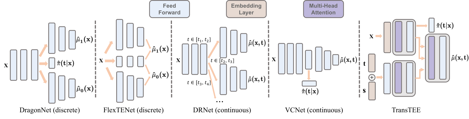
The systematic similarity of potential outcomes of different treatment groups is important for TEE [15]. Note that x is often high-dimensional while is not, which means naively feeding to MLPs is not favorable since the impacts of treatment tend to be lost. As a result, various architectures and regularizations have been proposed to enforce structural similarity and differences among treatment groups. However, they are limited to specific use cases, as shown in Section 2 and Figure 2. To remedy it, we use three simple yet effective design choices based on attention mechanisms. The resulting scalable framework TransTEE can tackle the problems of most existing treatment effect estimators (e.g., multiple/continuous/structured treatments, treatments interaction, and treatments with dosage) without ad-hoc architectural designs, e.g., multiple branches.
Preliminary. The main module in TransTEE is the attention layer [66]: given -dimensional query, key, and value matrices , attention mechanism computes the outputs as . In practice, multi-head attention is preferable to jointly attend to the information from different representation subspaces.
where and are learnable matrices.
4.1 Covariate and Treatment Embedding Layers
Treatment Embedding Layer. As illustrated in Figure 2 and Table. 1, as treatments are often of much lower dimension compared to covariates, to avoid missing the impacts of treatments, previous works (e.g., DragonNet [61], FlexTENet [15], DRNet [58]) assign covariates from different treatment groups to different branches, which is highly parameter inefficient. Besides, We analyze in Proposition 12 (Appendix D) that, for continuous treatments/dosages, the performance is affected by both number of branches and the value interval of treatment. However, almost all previous works on continuous treatment/dosage assume the treatment or dosage is in a fixed value interval e.g., and Figure 3 shows that prevalent works fail when tested under shifts of treatments. These two observations motivate us to use two learnable linear layers to project scalar treatments and dosages to -dimension vectors separately: , where . exists just when each treatment has a dosage parameter, otherwise, only treatment embedding is needed. When multiple () treatments act simultaneously, the projected matrix will be and when facing structural treatments (languages, graphs), the treatment embedding will be projected by language models and graph neural networks respectively. By using the treatment embeddings, TransTEE is shown to be (i) robust under treatment shifts, and (ii) parameter-efficient.
Covariates Embedding Layer. Different from previous works that embed all covariates by one fully connected layer, where the differences between covariates tend to be lost, it is difficult to study the function of an individual covariate in a sample. TransTEE learns different embeddings for each covariate, namely , and , where is the number of covariate. Covariates embedding enables us to study the effect of individual covariate on the outcome.
4.2 Covariate and Treatment Self-Attention
For covariates, prevalent methods represent covariates as a whole feature using MLPs, where pair-wise covariate interactions are lost when adjusting covariates. Therefore, we cannot study the effect of each covariate on the estimated result. In contrast, TransTEE processes each covariate embedding independently and model their interactions by self-attention layers. Namely,
where is the output of layer and BN is the BatchNorm layer. Simultaneously, the treatments and dosages embeddings are concatenated and projected to the latent dimension by a linear layer, which generates a new embedding . Then self-attention is applied
The self-attention layer for treatments enables treatment interactions, an important desideratum for S- and T-learners. Namely, TransTEE can model the scenario where multiple treatments are applied and attain strong practical utility, e.g., multiple prescriptions in healthcare or different financial measures in economics. This is an effective remedy for existing methods which are limited to settings where various treatments are not used simultaneously.
4.3 Treatment-Covariate Cross-Attention
One of the fundamental challenges of causal meta-learners is to model treatment-covariate interactions. TransTEE realizes this by a cross-attention module, treating as query and as key and value
where is the output of the last cross-attention layer and . The above interactions are particularly important for adjusting proper covariate or confounder sets for estimating treatment effects [65], which empirically yields suitable covariate adjustment principles (the Disjunctive Cause Criteria) [17, 65] about pre-treatment covariates and confounders as intuitively illustrated in Figure 1 and corroborated in our experiments.
Denote and the training objective is the mean square error (MSE) of the outcome regression:
| (1) |
Remark. We include an illustration of TransTEE by a concrete example in Appendix B. Note that, although the embedding technique and attention mechanisms are commonly used in Computer Vision, Neural Language Processing communities, it is not well understood how to guide the design of these modules for causal inference and why these techniques benefit TEE tasks are underexplored. In this work, through the flexible use of embedding and attention mechanisms, we design a strong TEE architecture, we further use conceptual analysis and empirical results to show the benefit brought by the used design choices. Besides, when combined with the strong modeling capacity of Transformers, TransTEE can be extended to high-dimensional data flexibly and effectively on structured data. The generalizability of the TransTEE also allows new applications like auditing language models beyond semi-synthetic settings as shown in the next section.
5 Experimental Results
We elaborate on basic experimental settings, results, analysis, and empirical studies in this section. See Appendix E for full details of all experimental settings and detailed definitions of metrics. See Appendix F for many more results and remarks.
| Methods | Vanilla (Binary) | Vanilla () | Extrapolation () | Vanilla () | Extrapolation () |
| TARNet | 0.3670 0.61112 | 2.0152 1.07449 | 12.967 1.78108 | 5.6752 0.53161 | 31.523 1.5013 |
| DRNet | 0.3543 0.60622 | 2.1549 1.04483 | 11.071 0.99384 | 3.2779 0.42797 | 31.524 1.50264 |
| FlexTENet | 0.2700 0.10000 | —— | —— | —— | —— |
| VCNet | 0.2098 0.18236 | 0.7800 0.61483 | nan | nan | nan |
| TransTEE | 0.0983 0.15384 | 0.1151 0.10289 | 0.2745 0.14976 | 0.1621 0.14443 | 0.2066 0.23258 |
| TransTEE+MLE | 0.1721 ± 0.40061 | 0.0877 0.03352 | 0.2685 0.17552 | 0.2079 0.17637 | 0.1476 0.07123 |
| TransTEE+TR | 0.1913 0.29953 | 0.0781 0.03243 | 0.2393 0.08154 | 0.1143 0.03224 | 0.0947 0.0824 |
| TransTEE+PTR | 0.2193 0.34667 | 0.0762 0.07915 | 0.2352 0.17095 | 0.1363 0.08036 | 0.1363 0.08035 |
5.1 Experimental Settings
Datasets. Since the true counterfactual outcome (or ADRF) are rarely available for real-world data, we use synthetic or semi-synthetic data for empirical evaluation. for continuous treatments, we use one synthetic dataset and two semi-synthetic datasets: the IHDP and News datasets. For treatment with continuous dosages, we obtain covariates from a real dataset TCGA [10] and generate treatments, where each treatment is accompanied by a dosage. The resulting dataset is named TCGA (D). Following [39], datasets with structured treatments include Small-World (SW), which contains uniformly sampled covariates and randomly generated Watts–Strogatz small-world graphs [71] as treatments, and TCGA (S), which uses gene expression of cancer patients [10] for covariates and molecules from the QM9 dataset [50] as treatments. For the study on language models, we use the Enriched Equity Evaluation Corpus (EEEC) [21].
Baselines. Baselines for continuous and binary treatments include TARnet [60], Dragonnet [61], DRNet [58], FlexTENet [15], and VCNet [47]. SCIGAN [9] is chosen as the baseline for continuous dosages. Besides, we revise DRNet [58], TARNet [60], and VCNet [47] to DRNet (D), TARNet (D), VCNet (D), respectively, which allow multiple treatments and dosages. Specifically, DRNet (D) has main flows, each corresponding to a treatment and is divided into branches for continuous dosage. Baselines for structured treatments include Zero [39], GNN [39], GraphITE [28], and SIN [39]. To compare the performance of different frameworks fairly, all of the models regress on the outcome with empirical samples without any regularization. For MLE training of the propensity score model, the objective is the negative log-likelihood: .
Evaluation Metric. For continuous and binary treatments, we use the average mean squared error on the test set. For structured treatments, following [39], we rank all treatments by their propensity in a descending order. Top treatments are selected and the treatment effect of each treatment pair is evaluated by unweighted/weighted expected Precision in Estimation of Heterogeneous Effect (PEHE) [39], where the WPEHE@K accounts for the fact that treatment pairs that are less likely to have higher estimation errors should be given less importance. For multiple treatments and dosages, AMSE is calculated over all dosage and treatment pairs, resulting in AMSED.
5.2 Case Study and Numerical Results
Case study on treatment distribution shifts We start by conducting a case study on treatment distribution shifts (Figure 3), and exploring an extrapolation setting in which the treatment may subsequently be administered at values never seen before during training. Surprisingly, we find that while standard results rely on constraining the values of treatments [47] and dosages [58] to a specific range, our methods perform surprisingly well when extrapolating beyond these ranges as assessed on several benchmarks. In comparison, other methods appear to be comparatively brittle in these same settings. See Appendix D for a detailed discussion.
Case study of propensity modeling. TransTEE is conceptually simple and effective. However, when the sample size is small, it becomes important to account for selection bias [3]. However, most existing regularizations can only be used when treatments are discrete [8, 40, 20]. Thus we propose two regularization variants for continuous treatment/dosages, which are termed Treatment Regularization (TR, ) and its probabilistic version Probabilistic Treatment Regularization (PTR, ) respectively. The overall model is trained in a adversarial pattern, namely . Specifically, a propensity score model parameterized by an MLP is learned by minimizing , and then the outcome estimators are trained by . To overcome selection biases, bilevel optimization enforces effective treatment effect estimation while modeling the discriminative propensity features to partial out parts of covariates that cause the treatment but not the outcome and dispose of nuisance variations of covariates [39]. Such a recipe can account for selection bias where and leave spurious correlations out, which can also be more robust under model misspecification especially in the settings that require extrapolation on treatment (see Table 2 and Appendix C for concrete formalisms and discussions.).
As in Table 2, Appendix Table 5 and Table 12, with the addition of adversarial training as well as TR and PTR, TransTEE’s estimation error with continuous treatments can be further reduced. Overall, TR is better in the continuous case with smaller treatment distribution shifts, while PTR is preferable when shifts are greater. Both TR and PTR cannot achieve performance gains in discrete cases. The superiority of TR and PTR in combination with TransTEE over comprehensive existing works, especially in semi-synthetic benchmarks like IHDP that may systematically favor some types of algorithms over others [13], also calls for more understanding of NNs’ inductive biases in treatment effect estimation problems of interest. Furthermore, the visualization of covariate selection in TR and PTR (Figure 4 , Table 4 and Appendix F) supports the idea that modeling the propensity score effectively promotes covariate adjustment and partials out the effects of the covariates on the treatment features. We also compare the training dynamic of different regularizations in Appendix F, where TR and PTR are further shown to be able to improve the convergence of TransTEE.
Continuous treatments. To evaluate the efficiency with which TransTEE estimates the average dose-response curve (ADRF), we compare it to other recent NN-based methods (Tables 2). By comparing the results in each column, we observe performance boosts for TransTEE. Further, TransTEE attains a much smaller error than baselines in cases where the treatment interval is not restricted to (e.g., ) and when the training and test treatment intervals are different (extrapolation). Interestingly, even vanilla TransTEE produces competitive performance compared to that of trained additionally using MLE, demonstrating the ability of TransTEE to effectively model treatments and covariates. The estimated ADRF curves on the IHDP and News datasets are shown in Figure 11 and Figure 13 in Appendix. TARNet and DRNet produce discontinuous ADRF estimators and VCNet only performs well when . However, TransTEE attains lower estimation error and preserves the continuity of ADRF on different treatment intervals.
| Correlation/Representation Based Baselines | Treatment Effect Estimators | |||||||
| TC | ATEGT | TReATE | CONEXP | INLP | TarNet | DRNet | VCNet | TransTEE |
| Gender | 0.086 | 0.125 | 0.02 | 0.313 | 0.0067 | 0.0088 | 0.0085 | 0.013 |
| [CI] | [0.082,0.09] | [0.110,0.14] | [0.0,0.05] | [0.304,0.321] | [0.0049, 0.0076] | [0.0084,0.009] | [0.0036, 0.0111] | [0.008, 0.0168] |
| Race | 0.014 | 0.046 | 0.08 | 0.591 | 0.005 | 0.006 | 0.003 | 0.0174 |
| [CI] | [0.012,0.016] | [0.038,0.054] | [0.02,0.014] | [0.578,0.605] | [0.0021, 0.0069] | [0.0047, 0.0081] | [0.0025, 0.0037] | [0.0113, 0.0238] |
Continuous dosage. In Table 5, we compare TransTEE against baselines on the TCGA (D) dataset with default treatment selection bias and dosage selection bias . As the number of treatments increases, TransTEE and its variants (with regularization term) consistently outperform the baselines by a large margin on both training and test data. TransTEE’s effectiveness is also shown in Appendix Figure 8, where the estimated ADRF curve of each treatment considering continuous dosages is plotted. Compared to baselines, TransTEE attains better results over all treatments. Stronger selection bias in the observed data makes estimation more difficult because it becomes less likely to see certain treatments or particular covariates. Taking into account different dosages and treatment selection biases, Appendix Figure 7 shows that as biases increase, TransTEE consistently performs the best.
Structured treatments. We compared the performance of TransTEE to baselines on the training and test set of both SW and TCGA datasets with varying degrees of treatment selection bias. The numerical results are shown in Appendix Table 13. The performance gain between GNN and Zero indicates that taking into account graph information significantly improves estimation. The results suggest that, overall, the performance of TransTEE is the best due to the strong modeling ability and advanced model structure to process high-dimensional treatments. SIN is the best model among these baselines. However, when the bias is equal to , SIN fails to achieve estimation results better than the Zero baseline. To evaluate the robustness of each model to varying levels of selection bias, performance curve with for the SW dataset and for the TCGA dataset are shown in Figure 14 and Figure 15 in Appendix. Considering both metrics, TransTEE outperforms baselines by a large margin across the entire range of evaluated treatment selection biases.
5.3 Analysis
Analysis of covariate adjustment of cross-attention module. TransTEE embeds each covariate independently and then model the interaction of treatments and covariates for prediction by cross-attention. The resulting interpretability of the covariate adjustment process using attention weights is one clear advantage over existing work. Thus we visualize the covariate selection results (cross-attention weights) in Figure 4. As elaborated in Appendix E.3, the IHDP dataset has covariates, which is divided into groups: , , and . influences both and , influences only , and influences only . Covariates in are named noisy covariates since they have no correlation with the treatment. Their causal relationships are illustrated in Figure 5. Interestingly, confounders are assigned higher weights while noisy covariates (those influence the outcome but are irrelevant to the treatment) lower , which matches the principles in [65] and corroborate the ability of TransTEE to estimate treatment effects in complex datasets by properly controlling pretreatment variables and confounders. Furthermore, Figure 4 shows that TransTEE consistently outperforms baselines across different numbers of noisy covariates.
| TransTEE | 0.27 | 0.37 | 0.36 |
| +TR | 0.59 | 0.20 | 0.21 |
| +PTR | 0.32 | 0.33 | 0.35 |
We further conduct 10 repetitions for TransTEE and its TR and PTR counterparts as reported in Table 4 (Appendix Figure 10 visualizes their cross-attention weights). Denote as the summation of weights assigned to respectively. We can see that, incorporated with both TR and PTR regularization, TransTEE assigns more weights to confounding covariates () and fewer weights on noisy covariates, which further verifies the compatibility of TransTEE with propensity score modeling since both TR and PTR improve confounding control. Moreover, TR is better than PTR since it also reduces by a larger margin. This observation gives a suggestion that we should systematically investigate TR and PTR in addition to comparing their numerical performance, especially in settings where the assumption of unconfoundedness is violated [18] and controlling instrumental variables will incur biases in TEE.
Amount of model parameters comparison. The experiment is to corroborate the conceptual comparison in Table 1. We find that the proposed TransTEE has consistently fewer parameters than baselines on all the settings as shown in Figure 4. Besides, increasing the number of treatments allows a more accurate approximation for continuous treatments/dosages, most of these baselines need to increase branches, which incurs manual efforts and parameter redundancy. However, TransTEE is much more efficient.
5.4 Empirical Study on Pre-trained Language Models
To evaluate the real-world utility of TransTEE, in this subsection, we demonstrate an initial attempt for auditing and debugging large pre-trained language models, an important use case in NLP that is beyond semi-synthetic settings and under-explored in the causal inference literature. Specifically, we use TransTEE to estimate the treatment effects for detecting the effects of domain-specific factors of variation (such as the change of subject’s attributes in a sentence) on the predictions of pre-trained language models. We experiment with BERT [42] (e.g., racial and gender-related nouns) over natural language on the (real) EEEC dataset. We use both the correlation/representation-based baselines introduced in [21] and implement treatment effect estimators (e.g., TARnet, DRNet, VCNet, and the proposed TransTEE).
Interestingly, results in Table 3 show that TransTEE effectively estimates the treatment effects of domain-specific variation perturbations even without substantive downstream fine-tuning on specialized datasets. TransTEE outperforms baselines adapted from MLP. Moreover, we showcase the top-k samples with the maximal/minimal ITE and analysis in Appendix F.3. The results show that TransTEE has the potential to serve as surrogate estimators for practical use cases in predicting model predictions [51]. For example, those identified samples can provide actionable insights, such as functions as contrast sets for analyzing and understanding LMs [26, 2] and TransTEE can estimate ATE to enforce invariant or fairness constraints for LMs [67] in a lightweight and efficient manner, which we leave for future work.
6 Concluding Remarks
In this work, we show attention mechanisms can be effective and versatile design choices for TEE tasks. Extensive experiments well verify the effectiveness and utility of the proposed TransTEE, which also imply that more challenging and unified evaluation alternatives of TEE are needed. Moreover, we hope that our findings can lay the groundwork for future work in developing advanced machine learning techniques like pre-training in large-scale observational data in estimating treatment effects, where TransTEE can serve as an effective backbone. Similar to almost all causal inference methods on observational data, one potential limitation of TransTEE is the reliance on the ignorability assumption. Therefore, an important future direction is extending TransTEE to settings with more complex causal graphs and generate identifiable causal functionals that are tractable for optimization [38] supported by identification theory. Since adjusting covariates without accounting for the causal graph might yield inaccurate or biased estimates of the causal effect [49], how to integrate TransTEE with domain knowledge [32] for alleviating its potential negative societal impacts in consequential decision making will also be important.
Acknowledgements
We thank Edward H. Kennedy and Hongyi Wang for helpful discussions and feedback.
References
- [1] Alberto Abadie and Guido W Imbens. Matching on the estimated propensity score. Econometrica, 2016.
- [2] Eldar David Abraham, Karel D’Oosterlinck, Amir Feder, Yair Ori Gat, Atticus Geiger, Christopher Potts, Roi Reichart, and Zhengxuan Wu. Cebab: Estimating the causal effects of real-world concepts on nlp model behavior. arXiv preprint arXiv:2205.14140, 2022.
- [3] Ahmed Alaa and Mihaela Schaar. Limits of estimating heterogeneous treatment effects: Guidelines for practical algorithm design. In ICML, 2018.
- [4] Ahmed M Alaa and Mihaela van der Schaar. Bayesian inference of individualized treatment effects using multi-task gaussian processes. In NeurIPS, 2017.
- [5] Ahmed M Alaa, Michael Weisz, and Mihaela Van Der Schaar. Deep counterfactual networks with propensity-dropout. arXiv, 2017.
- [6] Peter C Austin. An introduction to propensity score methods for reducing the effects of confounding in observational studies. Multivariate behavioral research, 2011.
- [7] Shai Ben-David, John Blitzer, Koby Crammer, Alex Kulesza, Fernando Pereira, and Jennifer Wortman Vaughan. A theory of learning from different domains. Machine learning, 2010.
- [8] Ioana Bica, Ahmed M Alaa, James Jordon, and Mihaela van der Schaar. Estimating counterfactual treatment outcomes over time through adversarially balanced representations. arXiv, 2020.
- [9] Ioana Bica, James Jordon, and Mihaela van der Schaar. Estimating the effects of continuous-valued interventions using generative adversarial networks. 2020.
- [10] Kyle Chang, Chad J Creighton, Caleb Davis, Lawrence Donehower, Jennifer Drummond, David Wheeler, Adrian Ally, Miruna Balasundaram, Inanc Birol, Yaron SN Butterfield, et al. The cancer genome atlas pan-cancer analysis project. Nat Genet, 2013.
- [11] Mark Chen, Jerry Tworek, Heewoo Jun, Qiming Yuan, Henrique Ponde de Oliveira Pinto, Jared Kaplan, Harri Edwards, Yuri Burda, Nicholas Joseph, Greg Brockman, et al. Evaluating large language models trained on code. arXiv, 2021.
- [12] Jonathan Crabbé, Alicia Curth, Ioana Bica, and Mihaela van der Schaar. Benchmarking heterogeneous treatment effect models through the lens of interpretability. arXiv preprint arXiv:2206.08363, 2022.
- [13] Alicia Curth, David Svensson, Jim Weatherall, and Mihaela van der Schaar. Really doing great at estimating CATE? a critical look at ML benchmarking practices in treatment effect estimation. In NeurIPS, 2021.
- [14] Alicia Curth and Mihaela van der Schaar. Nonparametric estimation of heterogeneous treatment effects: From theory to learning algorithms. In AISTATS, 2021.
- [15] Alicia Curth and Mihaela van der Schaar. On inductive biases for heterogeneous treatment effect estimation. In NeurIPS, 2021.
- [16] Ralph B D’Agostino. Propensity score methods for bias reduction in the comparison of a treatment to a non-randomized control group. Statistics in medicine, 1998.
- [17] Xavier De Luna, Ingeborg Waernbaum, and Thomas S Richardson. Covariate selection for the nonparametric estimation of an average treatment effect. Biometrika, 2011.
- [18] Peng Ding, TJ VanderWeele, and James M Robins. Instrumental variables as bias amplifiers with general outcome and confounding. Biometrika, 2017.
- [19] Alexey Dosovitskiy, Lucas Beyer, Alexander Kolesnikov, Dirk Weissenborn, Xiaohua Zhai, Thomas Unterthiner, Mostafa Dehghani, Matthias Minderer, Georg Heigold, Sylvain Gelly, et al. An image is worth 16x16 words: Transformers for image recognition at scale. 2021.
- [20] Xin Du, Lei Sun, Wouter Duivesteijn, Alexander Nikolaev, and Mykola Pechenizkiy. Adversarial balancing-based representation learning for causal effect inference with observational data. DMKD, 2021.
- [21] Amir Feder, Nadav Oved, Uri Shalit, and Roi Reichart. Causalm: Causal model explanation through counterfactual language models. Computational Linguistics, 2021.
- [22] Dylan J Foster and Vasilis Syrgkanis. Orthogonal statistical learning. arXiv preprint arXiv:1901.09036, 2019.
- [23] Constantine E Frangakis and Donald B Rubin. Principal stratification in causal inference. Biometrics, 2002.
- [24] Michele Jonsson Funk, Daniel Westreich, Chris Wiesen, Til Stürmer, M Alan Brookhart, and Marie Davidian. Doubly robust estimation of causal effects. American journal of epidemiology, 2011.
- [25] Yaroslav Ganin, Evgeniya Ustinova, Hana Ajakan, Pascal Germain, Hugo Larochelle, François Laviolette, Mario Marchand, and Victor Lempitsky. Domain-adversarial training of neural networks. JMLR, 2016.
- [26] Matt Gardner, Yoav Artzi, Victoria Basmov, Jonathan Berant, Ben Bogin, Sihao Chen, Pradeep Dasigi, Dheeru Dua, Yanai Elazar, Ananth Gottumukkala, et al. Evaluating models’ local decision boundaries via contrast sets. In EMNLP Findings, 2020.
- [27] Zhenyu Guo, Shuai Zheng, Zhizhe Liu, Kun Yan, and Zhenfeng Zhu. Cetransformer: Casual effect estimation via transformer based representation learning. In PRCV, 2021.
- [28] Shonosuke Harada and Hisashi Kashima. Graphite: Estimating individual effects of graph-structured treatments. In CIKM, 2021.
- [29] Jennifer L Hill. Bayesian nonparametric modeling for causal inference. Journal of Computational and Graphical Statistics, 2011.
- [30] Keisuke Hirano, Guido W Imbens, and Geert Ridder. Efficient estimation of average treatment effects using the estimated propensity score. Econometrica, 2003.
- [31] Kurt Hornik, Maxwell Stinchcombe, and Halbert White. Multilayer feedforward networks are universal approximators. Neural networks, 1989.
- [32] Guido W Imbens and Donald B Rubin. Causal inference in statistics, social, and biomedical sciences. Cambridge University Press, 2015.
- [33] Alon Jacovi and Yoav Goldberg. Towards faithfully interpretable nlp systems: How should we define and evaluate faithfulness? arXiv preprint arXiv:2004.03685, 2020.
- [34] Andrew Jaegle, Sebastian Borgeaud, Jean-Baptiste Alayrac, Carl Doersch, Catalin Ionescu, David Ding, Skanda Koppula, Daniel Zoran, Andrew Brock, Evan Shelhamer, Olivier J Henaff, Matthew Botvinick, Andrew Zisserman, Oriol Vinyals, and Joao Carreira. Perceiver IO: A general architecture for structured inputs & outputs. In ICLR, 2022.
- [35] Andrew Jaegle, Felix Gimeno, Andy Brock, Oriol Vinyals, Andrew Zisserman, and Joao Carreira. Perceiver: General perception with iterative attention. In ICML, 2021.
- [36] Fredrik Johansson, Uri Shalit, and David Sontag. Learning representations for counterfactual inference. In ICML, 2016.
- [37] Fredrik D Johansson, Uri Shalit, Nathan Kallus, and David Sontag. Generalization bounds and representation learning for estimation of potential outcomes and causal effects. arXiv, 2020.
- [38] Yonghan Jung, Jin Tian, and Elias Bareinboim. Learning causal effects via weighted empirical risk minimization. 2020.
- [39] Jean Kaddour, Yuchen Zhu, Qi Liu, Matt J Kusner, and Ricardo Silva. Causal effect inference for structured treatments. 2021.
- [40] Nathan Kallus. Deepmatch: Balancing deep covariate representations for causal inference using adversarial training. In ICML, 2020.
- [41] Joseph DY Kang and Joseph L Schafer. Demystifying double robustness: A comparison of alternative strategies for estimating a population mean from incomplete data. Statistical science, 2007.
- [42] Jacob Devlin Ming-Wei Chang Kenton and Lee Kristina Toutanova. Bert: Pre-training of deep bidirectional transformers for language understanding. In NAACL-HLT, 2019.
- [43] Sören R Künzel, Jasjeet S Sekhon, Peter J Bickel, and Bin Yu. Metalearners for estimating heterogeneous treatment effects using machine learning. PNAS, 2019.
- [44] Christos Louizos, Uri Shalit, Joris M Mooij, David Sontag, Richard S Zemel, and Max Welling. Causal effect inference with deep latent-variable models. In NeurIPS, 2017.
- [45] Shakir Mohamed and Balaji Lakshminarayanan. Learning in implicit generative models. arXiv, 2016.
- [46] David Newman. Bag of words data set. UCI Machine Learning Respository, 2008.
- [47] Lizhen Nie, Mao Ye, Qiang Liu, and Dan Nicolae. Vcnet and functional targeted regularization for learning causal effects of continuous treatments. 2021.
- [48] Sonali Parbhoo, Stefan Bauer, and Patrick Schwab. Ncore: Neural counterfactual representation learning for combinations of treatments. arXiv, 2021.
- [49] Judea Pearl. Causality. 2009.
- [50] Raghunathan Ramakrishnan, Pavlo O Dral, Matthias Rupp, and O Anatole Von Lilienfeld. Quantum chemistry structures and properties of 134 kilo molecules. Scientific data, 2014.
- [51] Marco Tulio Ribeiro, Sameer Singh, and Carlos Guestrin. " why should i trust you?" explaining the predictions of any classifier. In KDD, 2016.
- [52] Paul R Rosenbaum and Donald B Rubin. The central role of the propensity score in observational studies for causal effects. Biometrika, 1983.
- [53] Paul R Rosenbaum and Donald B Rubin. Reducing bias in observational studies using subclassification on the propensity score. JASA, 1984.
- [54] Donald B Rubin. Bayesian inference for causal effects: The role of randomization. The Annals of statistics, 1978.
- [55] Donald B Rubin. The design versus the analysis of observational studies for causal effects: parallels with the design of randomized trials. Statistics in medicine, 2007.
- [56] Donald B Rubin and Neal Thomas. Matching using estimated propensity scores: relating theory to practice. Biometrics, 1996.
- [57] Bernhard Schölkopf, Francesco Locatello, Stefan Bauer, Nan Rosemary Ke, Nal Kalchbrenner, Anirudh Goyal, and Yoshua Bengio. Toward causal representation learning. Proceedings of the IEEE, 2021.
- [58] Patrick Schwab, Lorenz Linhardt, Stefan Bauer, Joachim M Buhmann, and Walter Karlen. Learning counterfactual representations for estimating individual dose-response curves. In AAAI, 2020.
- [59] Patrick Schwab, Lorenz Linhardt, and Walter Karlen. Perfect match: A simple method for learning representations for counterfactual inference with neural networks. arXiv, 2018.
- [60] Uri Shalit, Fredrik D Johansson, and David Sontag. Estimating individual treatment effect: generalization bounds and algorithms. In ICML, 2017.
- [61] Claudia Shi, David Blei, and Victor Veitch. Adapting neural networks for the estimation of treatment effects. 2019.
- [62] Brian K Shoichet. Interpreting steep dose-response curves in early inhibitor discovery. Journal of medicinal chemistry, 2006.
- [63] Rahul Singh, Maneesh Sahani, and Arthur Gretton. Kernel instrumental variable regression. 2019.
- [64] Mark J Van Der Laan and Daniel Rubin. Targeted maximum likelihood learning. The international journal of biostatistics, 2006.
- [65] Tyler J VanderWeele. Principles of confounder selection. European journal of epidemiology, 2019.
- [66] Ashish Vaswani, Noam Shazeer, Niki Parmar, Jakob Uszkoreit, Llion Jones, Aidan N Gomez, Łukasz Kaiser, and Illia Polosukhin. Attention is all you need. In NeurIPS, 2017.
- [67] Victor Veitch, Alexander D’Amour, Steve Yadlowsky, and Jacob Eisenstein. Counterfactual invariance to spurious correlations in text classification. 2021.
- [68] Stefan Wager and Susan Athey. Estimation and inference of heterogeneous treatment effects using random forests. Journal of the American Statistical Association, 113(523):1228–1242, 2018.
- [69] Hao Wang, Hao He, and Dina Katabi. Continuously indexed domain adaptation. In ICML, 2020.
- [70] Haohan Wang, Zeyi Huang, Hanlin Zhang, Yong Jae Lee, and Eric Xing. Toward learning human-aligned cross-domain robust models by countering misaligned features. 2022.
- [71] Duncan J Watts and Steven H Strogatz. Collective dynamics of ‘small-world’networks. nature, 1998.
- [72] Jeffrey M Wooldridge. Introductory econometrics: A modern approach. Cengage learning, 2015.
- [73] Yifan Wu, Ezra Winston, Divyansh Kaushik, and Zachary Lipton. Domain adaptation with asymmetrically-relaxed distribution alignment. In ICML, 2019.
- [74] Guoqiang Xu, Cunxiang Yin, Yuchen Zhang, Yuncong Li, Yancheng He, Jing Cai, and Zhongyu Wei. Learning discriminative representation base on attention for uplift. In Pacific-Asia Conference on Knowledge Discovery and Data Mining, pages 200–211. Springer, 2022.
- [75] Chengxuan Ying, Tianle Cai, Shengjie Luo, Shuxin Zheng, Guolin Ke, Di He, Yanming Shen, and Tie-Yan Liu. Do transformers really perform bad for graph representation? 2021.
- [76] Jinsung Yoon, James Jordon, and Mihaela Van Der Schaar. Ganite: Estimation of individualized treatment effects using generative adversarial nets. In ICLR, 2018.
- [77] Shuxi Zeng, Serge Assaad, Chenyang Tao, Shounak Datta, Lawrence Carin, and Fan Li. Double robust representation learning for counterfactual prediction, 2020.
- [78] Hanlin Zhang, Yi-Fan Zhang, Weiyang Liu, Adrian Weller, Bernhard Schölkopf, and Eric P Xing. Towards principled disentanglement for domain generalization. CVPR, 2022.
- [79] Yao Zhang, Alexis Bellot, and Mihaela Schaar. Learning overlapping representations for the estimation of individualized treatment effects. In AISTATS, 2020.
- [80] Han Zhao, Shanghang Zhang, Guanhang Wu, José MF Moura, Joao P Costeira, and Geoffrey J Gordon. Adversarial multiple source domain adaptation. 2018.
Appendix
Table of Contents
Appendix A Extended Related Work
Propensity Score. Most related works fundamentally rely on strongly ignorable conditions. Still even under ignorability, treatments may be selectively assigned according to propensities that depend on the covariates. To overcome the impact of such confounding, many statistical methods [6] like covariate adjustment [6], matching [56, 1], stratification [23], reweighting [30], g-computation [32], have been proposed. More recent approaches include propensity dropout [5], and multi-task Gaussian process [4]. Explicitly modeling the propensity score, which reflects the underlying policy for assigning treatments to subjects, has also shown to be effective in reasoning about the unobserved counterfactual outcomes and accounting for confounding. Based upon it, double robust estimators and targeted regularization are proposed to guarantee the consistency of estimated treatment effects under misspecification of either the outcome or propensity score model [41, 24]. There are also works using adversarial training for balanced representations [8, 40, 20]. However, most traditional approaches are restricted to binary treatments and the capacity of NNs for such problems has not been fully leveraged.
Domain Adaptation There are some close connections between causal inference and domain adaptation, in particular, out-of-distribution robustness. Intuitively, traditional domain adversarial training learns representations that are indistinguishable from the domain classifier by minimizing the worst-domain empirical error [25, 80, 70, 78]. The algorithmic insights can be handily translated to the TEE domain [60, 37, 21]. Here we also have the desideratum that covariate representations should be balanced such that the selection bias is minimized and the effect is maximally determined by the treatment. Algorithmically, when the treatment is continuous, we connect our method to continuously indexed domain adaptation [69]. Our formulation and algorithm also serve to build connections to a diverse set of statistical thinking on causal inference and domain adaptation, of which much can be gained by mutual exchange of ideas [37]. Explicitly modeling the propensity score also seeks to connect causal inference with transfer learning to inspire domain adaptation methodology and holds the potential to handle a wider range of problems like hidden stratification in domain generalization, which we leave for future work.
Comparision between TransTEE and ANU [74]. (i) The model structure is different. ANU performs cross-attention between , and , and no self-attention is applied. However, TransTEE performs self-attention on respectively and then cross-attention is performed between . When facing high-dimensional data, such as texts, images, and graphs, without multiple self-attention layers on separately, the representations will be weak. That is why in machine translation, object detection, and segmentation tasks, the representations of images/texts will be firstly processed by multiple self-attention layers and then perform cross-attention with queries. We will verify this point in the following experiments. (ii) ANU cannot be applied to multi-treatment settings, which have been extensively studied recently [39, 9, 48]. The comparison experiments are in Section F.1.
Appendix B An Illustrative Example

To better understand the workflow with the above designs, we present a simple illustration here. Consider a use case in medicine effect estimation, where x contains patient information, e.g., Age, Sex, Blood Pressure (BP), and Previous infection condition (Prev) with a corresponding causal graph (Figure 1). medicines (treatments) are applied simultaneously and each medicine has a corresponding dosage. As shown in Figure 6, each covariate, treatment, and dosage will first be embedded to -dimension representation by a specific learnable embedding layer. Each treatment embedding will be concatenated with its dosage embedding and the concatenated feature will be projected by a linear layer to produce dimensional vectors. Self-attention modules optimizes these embeddings by aggregating contextual information. Specifically, attribute Prev is more related to age than sex, hence the attention weight of Prev feature to age feature is larger and the update of Prev feature will be more dependent on the age feature. Similarly, the interaction of multi-medicines is also attained by the self-attention module. The last Cross-attention module enables treatment-covariate interactions, which is shown in Figure 2 that, each medicine will assign a higher weight to relevant covariates especially confounders (BP) than irrelevant ones. Finally, we pool the resulting embedding and use one linear layer to predict the outcome.
Appendix C Details and Discussions about Propensity Score Modelling
We first discuss the fundamental differences and common goals between our algorithm and traditional ones: as a general approach to causal inference, TransTEE can be directly harnessed with traditional methods that estimate propensity scores by including hand-crafted features of covariates [32] to reduce biases through covariate adjustment [6], matching [56, 1], stratification [23], reweighting [30], g-computation [32], sub-classification [53], covariate adjustment [6], targeted regularization [64] or conditional density estimation [47] that create quasi-randomized experiments [16]. It is because the general framework provides an advantage to using an off-the-shelf propensity score regularizer for balancing covariate representations. Similar to the goal of traditional methods like inverse probability weighting and propensity score matching [6], which seeks to weigh a single observation to mimic the randomization effects with respect to the covariate from different treatment groups of interest.
Unlike previous works that use hand-crafted features or directly model the conditional density via maximum likelihood training, which is prone to high variance when handling high-dimensional, structured treatments [63] and can be problematic when we want to estimate a plausible propensity score from the generative model [45] (see the degraded performance of MLE in Table 2), TransTEE learns a propensity score network via minimax bilevel optimization. The motivations for adversarial training between and are three-fold: (i) it enforces the independence between treatment and covariate representations as shown in Proposition C, which serves as algorithmic randomization in place of costly randomized controlled trials [55] for overcoming selection bias [16, 32]; (ii) it explicitly models the propensity to refine treatment representations and promote covariate adjustment [39]; and (iii) taking an adversarial domain adaptation perspective, the methodology is effective for learning invariant representations and also regularizes to be invariant to nuisance factors and may perform better empirically on some classes of distribution shifts [25, 60, 80, 37, 69].
Based on the above discussion, when treatments are discrete, one might consider directly applying heuristic methods such as adversarial domain adaptation (see [25, 80] for algorithmic development guidelines). We note the heuristic nature of domain-adversarial methods (see [73] for clear failure cases) and a debunking of the common claim that [7] guarantees the robustness of such methods. Here, we focus on continuous TEE, a more general and challenging scenario, where we want to estimate ADRF, and propose two variants of as an adversary for the outcome regression objective in Eq. 1 accordingly. The process is shown in Eq. 2 below:
| (2) |
We refer to the above minimax game for algorithmic randomization in place of costly randomized controlled trials. Such algorithmic randomization based on neural representations using propensity score creates subgroups of different treated units as if they had been randomly assigned to different treatments such that conditional independence is enforced across strata and continuation, which approximates a random block experiment to the observed covariates [32].
Below, we introduce two variants of :
Treatment Regularization (TR) is a standard MSE over the treatment space given the predicted treatment and the ground truth
| (3) |
TR is explicitly matching the mean of the propensity score to that of the treatment. In an ideal case, should be uniformly distributed given different x. However, the above treatment regularization procedure only provides matching for the mean of the propensity score, which can be prone to bad equilibriums and treatment misalignment [69]. Thus, we introduce the distribution of and model the uncertainty rather than predicting a scalar :
Probabilistic Treatment Regularization (PTR) is a probabilistic version of TR that models the mean (with a slight abuse of notation) and the variance of the estimated treatment
| (4) |
The PTR matches the whole distribution, i.e. both the mean and variance, of the propensity score to that of the treatment, which can be preferable in certain cases.
| Methods | #Treatment=1 | #Treatment=2 | #Treatment=3 | |||
| In-Sample | Out-Sample | In-Sample | Out-Sample | In-Sample | Out-Sample | |
| SCIGAN | 5.6966 ± 0.0000 | 5.6546 ± 0.0000 | 2.0924 ± 0.0000 | 2.3067 ± 0.0000 | 4.3183 ± 0.0000 | 4.6231 ± 0.0000 |
| TarNet(D) | 0.7888 ± 0.0609 | 0.7908 ± 0.0606 | 1.4207 ± 0.0784 | 1.4206 ± 0.0777 | 3.1982 ± 0.5847 | 3.1920 ± 0.5746 |
| DRNet(D) | 0.8034 ± 0.0469 | 0.8052 ± 0.0466 | 1.3739 ± 0.0858 | 1.3738 ± 0.0853 | 2.8632 ± 0.4227 | 2.8558 ± 0.4143 |
| VCNET(D) | 0.1566 ± 0.0303 | 0.1579 ± 0.0301 | 0.2919 ± 0.0743 | 0.2918 ± 0.0737 | 0.6459 ± 0.1387 | 0.6493 ± 0.1397 |
| TransTEE | 0.0573 ± 0.0361 | 0.0585 ± 0.0358 | 0.0550 ± 0.0137 | 0.0556 ± 0.0129 | 0.2803 ± 0.0658 | 0.2768 ± 0.0639 |
| TransTEE + TR | 0.0495 ± 0.0176 | 0.0509 ± 0.0180 | 0.0663 ± 0.0268 | 0.0671 ± 0.0268 | 0.2618 ± 0.0737 | 0.2577 ± 0.0726 |
| TransTEE + PTR | 0.0343 ± 0.0096 | 0.0355 ± 0.0094 | 0.0679 ± 0.0252 | 0.0686 ± 0.0252 | 0.2645 ± 0.0702 | 0.2597 ± 0.0675 |
Equilibrium of the Minimax Game. We analyze that TR and PTR can align the first and second moment of continuous treatments at equilibrium respectively, and thus promote the independence between treatment and covariate x. To be clear, we denote and , which decompose the predictions into featurizers and predictors . For example, and can be the linear embedding layer and attention modules in our implementation. The propensity is computed on , an intermediate feature representation of x. Similarly, is computed from and . For the ease of our analysis below, we assume the predictors are fixed.
(The optimum of propensity score model) In the equilibrium of the game, assuming the outcome prediction model is fixed, then the optimum of TR is achieved when via matching the mean of propensity score and the marginal distribution and the optimum discriminator of PTR is achieved via matching both the mean and variance such that .
Proof.
The proof concerns the analysis of the equilibrium of the Minimax Game. It is a special case of [69] when there are only two players, i.e. and . We represent treatments explicitly and interpret the connections with combating selection biases. Given the fixed outcome regression model , the optimal propensity score model is
| (5) | ||||
The inner minimum is achieved at given the following quadratic form:
| (6) | ||||
We assume the above optimum condition of the propensity score model always holds with respect to the outcome regression model during training, then the minimax game in Eq. 2 can be converted to maximize the inner loop:
| (7) | ||||
Next we show the difference between Eq. 7 and the variance of the treatment :
| (8) | ||||
where the last inequality is determined by Jensen’s inequality and the convexity of . The optimum is achieved when is constant w.r.t and so .
The proof process for PTR is similar but includes the derivation of variance matching.
| (9) |
where and denote and respectively for brevity. The first term can be reduced to a constant given the definition of variance:
| (10) | ||||
The second term can be upper bounded by using Jensen’s inequality:
| (11) | ||||
Appendix D Analysis of the Failure Cases over Treatment Distribution Shifts
As shown in Figure 3 (a,c), with the shifts of the treatment interval, the estimation performance of DRNet and TARNet decline significantly. VCNet achieves estimation error when partly because its hand-craft projection matrix can only process values near . Another problem brought by this assumption is the extrapolation dilemma, which can be seen in Figure 3(b). When training on , these discrete approximation methods cannot transfer to new distribution . These unseen treatments are rounded down to the nearest neighbors in and be seemed the same as . We conduct ablation about the treatment embedding as in Table 6 in Appendix. Such a simple fix (VCNet+Embeddings) removes the demand on a fixed interval constraint to treatments and attains superior performance on both interpolation and extrapolation settings. The result clearly shows the pitfalls of hand-crafted feature mapping for TEE. We highlight that it is neglected by most existing works [58, 47, 61, 27]. Extrapolation is still a challenging open problem. We can see that no existing work does well when training and test treatment intervals have big gaps. However, the empirical evidence validates the improved effectiveness of TransTEE that uses learnable embeddings to map continuous treatments to hidden representations.
Below we show the assumption that the value of treatments or dosages are in a fixed interval is sub-optimal and thus these methods get poor extrapolation results. For simplicity, we only consider a data sample that has only one continuous treatment and the result is similar for continuous dosage. {prop} Given a data sample , where . Assume is a L-Lipschitz function over , namely . Partitioning uniformly into sub-interval, and then get . Previous studies most rounding down a treatment to its nearest value in (either or ) and use branches to approximate the entire continuum . The approximation error can be bounded by
| (12) | ||||
The bound is affected by both the number of branches and treatment interval . However, as far as we know, most previous works ignore the impacts of the treatment interval and adopt a simple but much stronger assumption that treatments are all in the interval [47] or a fixed interval [58]. These observations well manifest the motivation of our general framework for TEE without the need for treatment-specific architectural designs.
| Methods | Vanilla | Vanilla () | Extrapolation () | Extrapolation () |
| TARNet [60] | 0.045 0.0009 | 0.3864 0.04335 | 0.0984 0.02315 | 0.3647 0.03626 |
| DRNet [58] | 0.042 0.0009 | 0.3871 0.03851 | 0.0885 0.00094 | 0.3647 0.03625 |
| VCNet[47] | 0.018 0.0010 | nan | 0.0669 0.05227 | nan |
| VCNet+Embeddings | 0.013 0.00465 | 0.0167 0.01150 | 0.0118 0.00482 | 0.0178 0.00887 |
Appendix E Additional Experimental Setups
All the assets (i.e., datasets and the codes for baselines) we use include a MIT license containing a copyright notice and this permission notice shall be included in all copies or substantial portions of the software. We conduct all the experiments on a machine with i7-8700K CPU, 32G RAM, and four Nvidia GeForce RTX2080Ti (10GB) GPU cards.
E.1 Detail Evaluation Metrics.
| (13) |
| (14) | ||||
| (15) |
E.2 Network Structure and Parameter Setting
Table. 7 and Table. 8 show the detail of TransTEE architecture and hyper-parameters. For all the synthetic and semi-synthetic datasets, we tune parameters based on 20 additional runs. In each run, we simulate data, randomly split it into training and testing, and use AMSE on testing data for evaluation. For fair comparisons, in all experiments, the model size of TransTEE is less than or similar to the baselines.
| Module | Covariates | Treatment |
| Embedding Layer | ||
| Output Size | Emb | |
| Self-Attention | ||
| Output Size | ||
| Cross-Attention | ||
| Output Size | ||
| Projection Layer | ||
| Output Size | ||
| Dataset | Bsz | # Emb | # Layers | # Heads | Lr | Lr. S |
| Simu | 500 | 10 | 1 | 2 | 0.01 | Cos |
| IHDP | 128 | 10 | 1 | 2 | 0.0005 | Cos |
| News | 256 | 10 | 1 | 2 | 0.01 | Cos |
| SW | 500 | 16 | 1 | 2 | 0.01 | None |
| TCGA | 1000 | 48 | 3 | 4 | 0.01 | None |
E.3 Simulation details.
Synthetic Dataset [47]. The synthetic dataset contains 500 training points and 200 testing points. Data is generated as follows: , where is the -th dimension of , and
where .
for treatment in , we revised it to ,
IHDP [29] is a semi-synthetic dataset containing 25 covariates, 747 observations and binary treatments. For treatments in , we follow VCNet [47] and generate treatments and responses by:
where , is the index set of continuous features, , and . Here ,. To allow comparison on various treatment intervals , treatments and responses are generated by:
where the orange part is the only different compared to the generalization of vanilla IHDP dataset (). Note that only impacts outcome that serves to be noisy covariates; contains pre-treatment covariates that only impact treatments, which also serve to be instrumental variables. This allows us to observe the improvement using TransTEE when noisy covariates exist. Following [29] covariates are standardized with mean and standard deviation .
News. The News dataset consists of 3000 randomly sampled news items from the NY Times corpus [46] and was originally introduced as a benchmark in the binary treatment setting. We generate the treatment and outcome in a similar way as [47] but with a dynamic range or treatment intervals . We first generate and then set . Given , we generate from .And we generate the outcome by
TCGA (D) [9] We obtain covariates from a real dataset The Cancer Genomic Atlas (TCGA) and consider treatments, where each treatment is accompanied by one dosage and a set of parameters, . For each run, we randomly sample a vector, and then set where is Euclidean norm. The shape of the response curve for each treatment, is given in Table 9. We add noise to the outcomes. Interventions are assigned by sampling a dosage, , for each treatment from a beta distribution, . controls the dosage selection bias ( gives the uniform distribution). , where is the optimal dosage33 3 For symmetry, if , we sample from Beta where is set as though . for treatment . We then assign a treatment according to where increasing increases selection bias, and leads to random assignments. The factual intervention is given by . Unless otherwise specified, we set and .
| Treatment | Dose-Response | Optimal dosage |
| 1 | ||
| 2 | ||
| 3 |
For structural treatments, we first define the Baseline effect [9]. For each run of the experiment, we randomly sample a vector , and set , where is the Euclidean norm. The baseline effect is defined as
Small-World [39]. -dimensional multivariate covariates are uniformly sampled according to . There are units in the in-sample dataset and in the out-sample one. Graph interventions For each graph intervention, a number of nodes between and are uniformly sampled, the number of neighbors for each node is between and , and the probability of rewiring each edge is between and . Watts–Strogatz small-world graphs are repeatedly generated until a connected one is get. Each vertex has one feature, i.e. its degree of centrality. A graph’s node connectivity is denoted as and its average shortest path length as . Similar for the baseline effect, two randomly sampled vectors are generated. Then, given an assigned graph treatment and a covariate vector , the outcome is generated by
TCGA (S) [39] We use gene expression measurements of cancer patients for covariates. The in-sample and datasets consist of units and the out-sample one of units, respectively. Each unit is a covariate vector and these units are split randomly into in- and out-sample datasets in each run randomly. For each covariate vector , its -dimensional PCA components is computed. Graph interventions We randomly sample molecules from the Quantum Machine 9 (QM9) dataset [50] (with k molecules in total) in each run. We create a relational graph, where each node corresponds to an atom and consists of atom features. We label each edge corresponding to the chemical bond types, e.g., single, double, triple, and aromatic bonds. We collect molecule properties in a vector , which is denoted as the assigned molecule treatment. Finally, we generate outcomes by
Enriched Equity Evaluation Corpus (EEEC) [21] consists of English sentences and the label of each sentence is the mood state it conveys. The task is also known as Profile of Mood States (POMS). Each sentence in the dataset is created using one of templates, with placeholders for a person’s name and the emotion, e.g., “Person made me feel emotional state word.”. A list of common names that are tagged as male or female, and as African-American or European will be used to fill the placeholder (Person). One of four possible mood states: Anger, Sadness, Fear and Joy is used to fill the emotion placeholder. Hence, EEEC has two kinds of counterfactual examples, which are Gender and Race. For the Gender case, it changes the name and the Gender pronouns in the example and switches them, such that for the original example: "It was totally unexpected, but Roger made me feel pessimistic." it will have the counterfactual example:“It was totally unexpected, but Amanda made me feel pessimistic.” For the Race concept, it creates counterfactuals such that for the original example “Josh made me feel uneasiness for the first time ever in my life.”, the counterfactual example is: “Darnell made me feel uneasiness for the first time ever in my life.”. For each counterfactual example, the person’s name is taken at random from the pre-existing list corresponding to its type.
Appendix F Additional Experimental Results
F.1 Comparision between TransTEE and ANU [74]
We implement ANU and evaluate it in the same settings and show that is inferior compared to the proposed TransTEE as follows. Specifically, we compare the attentive neural uplift model (ANU) [74] with ours in the following two settings. (1) IHDP dataset in Table 10 in the main manuscript. We adjust the layers of ANU such that the total parameters of ANU and TransTEE are similar. The result is shown in the following table. With the usage of treatment embeddings, ANU is shown to be more robust than VCNet and DRNet when a treatment shift occurs. However, in both the binary treatment setting and continuous treatment settings, TransTEE performs better than ANU.
| Methods | Vanilla (Binary) | Vanilla (h = 1) | Extrapolation (h = 2) |
| DRNet | 0.3543 ± 0.6062 | 2.1549 ± 1.04483 | 11.071 ± 0.9938 |
| VCNet | 0.2098 ± 0.18236 | 0.7800 ± 0.6148 | NAN |
| ANU [74] | 0.1482 ± 0.17362 | 0.2147± 0.32451 | 0.4244 ± 0.19832 |
| TransTEE | 0.0983 ± 0.15384 | 0.1151 ± 0.1028 | 0.2745 ± 0.1497 |
(2) We further evaluate the real-world utility of ANU [74] and the experimental setting is detailed in Section 5.4 in the main paper. Covariates here are long sentences. Thanks to the use of self-attention modules, TransTEE can achieve better estimation results compared to baselines (Table 11). For AHU, no self-attention layer is applied, and the final estimation is inaccurate, which verifies the superiority of the proposed framework.
| Correlation/Representation Based Baselines | Treatment Effect Estimators | ||||||||
| TC | ATEGT | TReATE | CONEXP | INLP | CausalBERT | TarNet | DRNet | ANU | TransTEE |
| Gender | 0.086 | 0.125 | 0.02 | 0.313 | 0.179 | 0.0067 | 0.0088 | 0.184 | 0.013 |
| Race | 0.014 | 0.046 | 0.08 | 0.591 | 0.213 | 0.005 | 0.006 | 0.093 | 0.0174 |
F.2 Additional Numerical Results and Ablation Studies
| Methods | Vanilla | Vanilla () | Extrapolation () | Extrapolation () |
| TARNet | 0.082 0.019 | 0.956 0.041 | 0.716 0.038 | 0.847 0.053 |
| DRNet | 0.083 0.032 | 0.956 0.041 | 0.703 0.038 | 0.834 0.053 |
| VCNet | 0.013 0.005 | nan | nan | nan |
| TransTEE | 0.010 0.004 | 0.017 0.008 | 0.024 0.017 | 0.029 0.019 |
| TransTEE+TR | 0.011 0.003 | 0.016 0.008 | 0.019 0.008 | 0.028 0.002 |
| TransTEE+PTR | 0.011 0.004 | 0.014 0.007 | 0.022 0.008 | 0.029 0.016 |
Choice of the balancing weight for treatment regularization. To understand the effect of propensity score modeling, we conduct an ablation study on the balancing weights of both TR and PTR. Figure 9 presents the results of the experiments on the IHDP dataset. The main observation is that both TR and PTR with a proper regularization strength consistently improve estimation compared to TransTEE without regularization. The best performers are achieved when is for both two methods, which shows that the best balancing parameter ( in our experiments.) for these two regularization terms should be searched carefully. Besides, training both the treatment predictor and the feature encoder simultaneously in a zero-sum game is difficult and sometimes unstable (shown in Figure 9 right)
Robustness to noisy covariates. We manipulate to generate datasets with different noisy covariates, e.g., when the number of covariates that only influence the outcome is , , and , when the number of covariates that influence the outcome is , , and . Figure Figure 4 shows that, as the number of covariates that only influence the outcome increases, both TARNet and DRNet become better estimators, however, VCNet performs worse and even inferior to TARNet and DRNet when the number is large than . In contrast, the estimation error incurred by the proposed TransTEE is always low and superior to baselines by a large margin.
Comparison of MLE or adversarial propensity score modeling on the propensity score. Seeing results in Table 2, additionally combine TransTEE with maximum likelihood training of does provide some performance gains. However, an adversarially trained -model can be significantly better, especially for extrapolation settings. The results well manifest the effectiveness of TR and PTR in reducing selection bias and improving estimation performance. In fact, approaches like TMLE are not robust if the initial estimator is poor [61].
Training dynamics comparison of different regularization terms. Here we compare four regularization terms, which are TransTEE with no regularization, TransTEE+TR, TransTEE+PTR, and TransTEE+MTL. TransTEE+MTL is a simple Multi-Task Learning strategy, which uses during training without an adversarial game. As shown in Figure 12, without adversarial training, TransTEE+MTL quickly attains low treatment estimation error but further oscillates and converge with a high error, and both the outcome regression error and MSE in the test set remain high. In contrast, TR and PTR make TransTEE converge faster and attain lower test MSE. Overall, PTR consistently works the best and its low treatment regression error shows that estimates an accurate propensity score.
F.3 Showcase of sentences and counterfactual counterparts with the maximal/minimal ATEs.
Table 14 showcases the top- samples with the maximal/ minimal ATEs. Interestingly, we can see most sentences with a large ATE have similar patterns, that is “ clause , but/and Person made me feel Adj ”. Besides, most sentences with a large ATE have a small length, which is words on average. By contrast, sentences with small ATEs follow other patterns and are longer, which is on average. Consider the effect of Race, Table 15 showcases the top- samples. Similarly, there are also some dominant patterns that have pretty high or low ATEs and the average length of sentences with high ATEs is smaller than sentences with low ATEs (). Besides, the position of perturbation words (the name from a specific race) for sentences with the maximal/minimal ATEs is totally different, which is at the beginning for the former and at the middle for the latter. Namely, TransTEE helps us mitigate spurious correlations that exist in model prediction, e.g., length of sentences, the position of perturbation words, certain sentence patterns and is useful in mitigating undesirable bias ingrained in the data. Besides, a well-optimized TransTEE is able to estimate the effect of every sentence and is of great benefit for model interpretation and analysis especially under high inference latency.
| Method | SW | TCGA (Bias=0.1) | TCGA (Bias=0.3) | TCGA (Bias=0.5) | ||||
| In-sample | Out-sample | In-sample | Out-sample | In-sample | Out-sample | In-sample | Out-sample | |
| WPEHE@2 | ||||||||
| Zero | 41.72 ± 0.00 | 49.69 ± 0.00 | 13.93 ± 0.00 | 13.13 ± 0.00 | 13.93 ± 0.00 | 13.13 ± 0.00 | 13.93 ± 0.00 | 13.61 ± 0.00 |
| GNN | 17.38 ± 0.01 | 24.53 ± 0.01 | 10.90 ± 7.71 | 10.91 ± 7.71 | 13.58 ± 0.18 | 13.22 ± 0.18 | 12.86 ± 0.38 | 14.62 ± 0.91 |
| GraphITE | 17.37 ± 0.01 | 24.56 ± 0.02 | 15.04 ± 0.20 | 14.96 ± 0.30 | 13.49 ± 0.23 | 13.70 ± 0.52 | 12.41 ± 0.02 | 14.38 ± 0.30 |
| SIN | 15.79 ± 1.72 | 28.78 ± 4.54 | 46.47 ± 2.19 | 54.41 ± 7.81 | 7.93 ± 0.79 | 11.04 ± 1.52 | 10.31 ± 0.93 | 14.09 ± 2.14 |
| TransTEE | 14.74 ± 0.09 | 21.78 ± 1.07 | 9.07 ± 2.15 | 9.33 ± 2.13 | 7.54 ± 3.60 | 8.37 ± 3.64 | 9.52 ± 3.59 | 10.10 ± 3.79 |
| WPEHE@3 | ||||||||
| Zero | 40.75 ± 0.00 | 43.76 ± 0.00 | 13.93 ± 0.00 | 13.61 ± 0.00 | 13.93 ± 0.00 | 13.61 ± 0.00 | 13.61 ± 0.00 | 14.14 ± 0.00 |
| GNN | 18.26 ± 0.00 | 20.91 ± 0.01 | 10.75 ± 7.60 | 10.91 ± 7.72 | 13.63 ± 0.18 | 13.58 ± 0.19 | 12.92 ± 0.33 | 15.29 ± 1.04 |
| GraphITE | 18.27 ± 0.01 | 20.95 ± 0.02 | 14.88 ± 0.19 | 15.12 ± 0.29 | 13.49 ± 0.22 | 14.19 ± 0.43 | 12.56 ± 0.01 | 15.18 ± 0.31 |
| SIN | 18.15 ± 1.97 | 23.62 ± 3.93 | 45.29 ± 2.33 | 53.72 ± 8.09 | 7.94 ± 0.75 | 11.53 ± 1.59 | 10.89 ± 1.07 | 14.27 ± 1.92 |
| TransTEE | 15.30 ± 1.12 | 18.73 ± 2.09 | 9.07 ± 2.02 | 9.58 ± 2.04 | 7.58 ± 3.62 | 8.65 ± 3.75 | 9.64 ± 3.56 | 10.59 ± 3.88 |
| WPEHE@4 | ||||||||
| Zero | 45.74 ± 0.00 | 44.95 ± 0.00 | 14.14 ± 0.00 | 13.75 ± 0.00 | 14.14 ± 0.00 | 13.75 ± 0.00 | 13.75 ± 0.00 | 14.31 ± 0.00 |
| GNN | 22.09 ± 0.01 | 23.01 ± 0.01 | 10.87 ± 7.69 | 10.88 ± 7.69 | 13.87 ± 0.18 | 13.71 ± 0.19 | 13.13 ± 0.34 | 15.47 ± 1.05 |
| GraphITE | 22.12 ± 0.00 | 23.03 ± 0.02 | 15.05 ± 0.18 | 15.14 ± 0.28 | 13.64 ± 0.20 | 14.30 ± 0.35 | 12.77 ± 0.02 | 15.38 ± 0.30 |
| SIN | 22.14 ± 2.30 | 23.70 ± 3.67 | 44.72 ± 2.35 | 53.12 ± 8.09 | 7.99 ± 0.73 | 11.66 ± 1.59 | 11.38 ± 1.04 | 14.37 ± 1.83 |
| TransTEE | 18.99 ± 0.83 | 19.65 ± 1.97 | 9.09 ± 1.97 | 9.66 ± 2.01 | 7.67 ± 3.70 | 8.71 ± 3.78 | 9.78 ± 3.63 | 10.74 ± 3.91 |
| WPEHE@5 | ||||||||
| Zero | 49.19 ± 0.00 | 45.96 ± 0.00 | 14.31 ± 0.00 | 13.95 ± 0.00 | 14.31 ± 0.00 | 13.95 ± 0.00 | 13.95 ± 0.00 | 14.47 ± 0.00 |
| GNN | 24.18 ± 0.01 | 24.20 ± 0.01 | 10.99 ± 7.77 | 10.97 ± 7.76 | 13.98 ± 0.17 | 13.92 ± 0.18 | 13.31 ± 0.37 | 15.67 ± 1.05 |
| GraphITE | 24.22 ± 0.01 | 24.22 ± 0.03 | 15.24 ± 0.19 | 15.29 ± 0.28 | 13.68 ± 0.17 | 14.37 ± 0.37 | 12.95 ± 0.03 | 15.59 ± 0.30 |
| SIN | 25.48 ± 3.02 | 25.44 ± 3.50 | 44.55 ± 2.35 | 52.78 ± 8.04 | 8.10 ± 0.75 | 11.76 ± 1.59 | 11.75 ± 1.22 | 14.59 ± 1.84 |
| TransTEE | 20.16 ± 0.42 | 21.08 ± 1.78 | 9.17 ± 1.96 | 9.72 ± 2.00 | 7.76 ± 3.75 | 8.80 ± 3.82 | 9.91 ± 3.66 | 10.89 ± 3.94 |
| WPEHE@6 | ||||||||
| Zero | 49.95 ± 0.00 | 50.10 ± 0.00 | 14.47 ± 0.00 | 14.04 ± 0.00 | 14.47 ± 0.00 | 14.04 ± 0.00 | 14.04 ± 0.00 | 14.53 ± 0.00 |
| GNN | 25.13 ± 0.00 | 26.93 ± 0.01 | 11.11 ± 7.86 | 11.02 ± 7.79 | 14.07 ± 0.22 | 14.11 ± 0.18 | 13.45 ± 0.38 | 15.76 ± 1.04 |
| GraphITE | 25.17 ± 0.02 | 26.94 ± 0.02 | 15.40 ± 0.19 | 15.37 ± 0.28 | 13.74 ± 0.12 | 14.58 ± 0.38 | 13.09 ± 0.04 | 15.68 ± 0.29 |
| SIN | 27.07 ± 2.98 | 28.11 ± 3.51 | 44.48 ± 2.35 | 52.54 ± 7.99 | 8.22 ± 0.75 | 11.82 ± 1.58 | 11.97 ± 1.19 | 14.74 ± 1.86 |
| TransTEE | 21.32 ± 0.79 | 22.99 ± 1.43 | 9.23 ± 1.95 | 9.77 ± 1.99 | 7.80 ± 3.83 | 8.84 ± 3.89 | 10.01 ± 3.70 | 10.96 ± 3.95 |
| WPEHE@7 | ||||||||
| Zero | 55.40 ± 0.00 | 58.42 ± 0.00 | 14.53 ± 0.00 | 14.09 ± 0.00 | 14.53 ± 0.00 | 14.09 ± 0.00 | 14.53 ± 0.00 | 14.09 ± 0.00 |
| GNN | 29.30 ± 0.03 | 32.15 ± 0.03 | 11.16 ± 7.89 | 11.06 ± 7.82 | 14.12 ± 0.21 | 14.14 ± 0.18 | 13.51 ± 0.38 | 15.81 ± 1.03 |
| GraphITE | 29.34 ± 0.01 | 32.16 ± 0.01 | 15.47 ± 0.19 | 15.42 ± 0.28 | 13.97 ± 0.08 | 14.69 ± 0.40 | 13.16 ± 0.04 | 15.74 ± 0.29 |
| SIN | 31.07 ± 3.07 | 34.17 ± 3.41 | 44.45 ± 2.37 | 52.40 ± 7.98 | 8.28 ± 0.74 | 11.85 ± 1.58 | 12.11 ± 1.18 | 14.83 ± 1.87 |
| TransTEE | 24.71 ± 0.41 | 25.84 ± 0.73 | 9.27 ± 1.94 | 9.81 ± 1.99 | 7.82 ± 3.84 | 8.89 ± 3.89 | 10.06 ± 3.71 | 11.01 ± 3.95 |
| WPEHE@8 | ||||||||
| Zero | 57.99 ± 0.00 | 66.78 ± 0.00 | 14.61 ± 0.00 | 14.14 ± 0.00 | 14.60 ± 0.00 | 14.12 ± 0.00 | 14.61 ± 0.00 | 14.14 ± 0.00 |
| GNN | 31.41 ± 0.03 | 37.57 ± 0.05 | 11.22 ± 7.93 | 11.09 ± 7.85 | 14.19 ± 0.25 | 14.20 ± 0.18 | 13.58 ± 0.38 | 15.87 ± 1.02 |
| GraphITE | 31.45 ± 0.01 | 37.58 ± 0.00 | 15.55 ± 0.19 | 15.47 ± 0.28 | 14.30 ± 0.04 | 14.85 ± 0.43 | 13.23 ± 0.04 | 15.78 ± 0.28 |
| SIN | 33.58 ± 3.37 | 40.83 ± 3.64 | 44.48 ± 2.38 | 52.34 ± 7.97 | 8.33 ± 0.74 | 11.87 ± 1.57 | 12.22 ± 1.17 | 14.91 ± 1.89 |
| TransTEE | 26.48 ± 0.27 | 32.40 ± 0.85 | 9.31 ± 1.94 | 9.85 ± 1.99 | 7.88 ± 3.84 | 8.90 ± 3.90 | 10.10 ± 3.72 | 11.04 ± 3.96 |
| WPEHE@9 | ||||||||
| Zero | 62.52 ± 0.00 | 64.61 ± 0.00 | 14.66 ± 0.00 | 14.20 ± 0.00 | 14.61 ± 0.00 | 14.14 ± 0.00 | 14.66 ± 0.00 | 14.20 ± 0.00 |
| GNN | 34.13 ± 0.04 | 36.48 ± 0.04 | 11.26 ± 7.96 | 11.13 ± 7.87 | 14.21 ± 0.24 | 14.22 ± 0.17 | 13.63 ± 0.38 | 15.92 ± 1.01 |
| GraphITE | 34.17 ± 0.02 | 36.49 ± 0.01 | 15.60 ± 0.19 | 15.53 ± 0.28 | 14.35 ± 0.04 | 14.90 ± 0.43 | 13.28 ± 0.04 | 15.83 ± 0.28 |
| SIN | 36.79 ± 3.35 | 40.99 ± 5.14 | 44.47 ± 2.39 | 52.31 ± 7.97 | 8.36 ± 0.74 | 11.90 ± 1.57 | 12.40 ± 1.23 | 15.08 ± 1.80 |
| TransTEE | 28.84 ± 0.23 | 31.40 ± 0.71 | 9.34 ± 1.94 | 9.88 ± 2.00 | 7.90 ± 3.85 | 8.94 ± 3.91 | 10.14 ± 3.73 | 11.08 ± 3.97 |
| WPEHE@10 | ||||||||
| Zero | 62.65 ± 0.00 | 65.59 ± 0.00 | 14.69 ± 0.00 | 14.23 ± 0.00 | 14.69 ± 0.00 | 14.23 ± 0.00 | 14.69 ± 0.00 | 14.23 ± 0.00 |
| GNN | 34.26 ± 0.04 | 37.65 ± 0.04 | 11.28 ± 7.98 | 11.16 ± 7.89 | 14.29 ± 0.22 | 14.32 ± 0.18 | 13.66 ± 0.38 | 15.96 ± 1.01 |
| GraphITE | 34.30 ± 0.02 | 37.66 ± 0.00 | 15.64 ± 0.19 | 15.56 ± 0.28 | 14.38 ± 0.04 | 14.93 ± 0.43 | 13.31 ± 0.04 | 15.87 ± 0.27 |
| SIN | 37.08 ± 3.35 | 41.79 ± 5.21 | 44.49 ± 2.40 | 52.28 ± 7.96 | 8.39 ± 0.74 | 11.92 ± 1.58 | 12.49 ± 1.22 | 15.13 ± 1.81 |
| TransTEE | 28.89 ± 0.19 | 32.25 ± 0.69 | 9.36 ± 1.93 | 9.90 ± 2.00 | 7.94 ± 3.87 | 8.95 ± 3.92 | 10.16 ± 3.74 | 11.10 ± 3.98 |
| Sentences with The Maximal ATEs | |||
| Index | Sentence | ATE | |
| 1 | It was totally unexpected, but Roger made me feel pessimistic. | 0.6393 | |
| 2 | We went to the restaurant, and Alphonse made me feel frustration. | 0.578 | |
| 3 | It was totally unexpected, but Amanda made me feel pessimistic. | 0.5109 | |
| 4 | We went to the university, and my husband made me feel angst. | 0.4538 | |
| 5 | It is far from over, but so far i made Jasmine feel frustration. | 0.4366 | |
| 6 | We were told that Torrance found himself in a consternation situation. | 0.4203 | |
| 7 | We went to the university, and my son made me feel revulsion. | 0.399 | |
| 8 | To our amazement, the conversation with my aunt was dejected. | 0.3952 | |
| 9 | To our amazement, the conversation with my aunt was dejected. | 0.3952 | |
| Factual | 10 | We went to the supermarket, and Roger made me feel uneasiness. | 0.3752 |
| 1 | It was totally unexpected, but Amanda made me feel pessimistic. | 0.6393 | |
| 2 | We went to the school, and Latisha made me feel frustration. | 0.578 | |
| 3 | It was totally unexpected, but Roger made me feel pessimistic. | 0.5109 | |
| 4 | We went to the market, and my daughter made me feel angst. | 0.4538 | |
| 5 | It is far from over, but so far i made Jamel feel frustration. | 0.4366 | |
| 6 | We were told that Tia found herself in a consternation situation. | 0.4203 | |
| 7 | We went to the hairdresser, and my sister made me feel revulsion. | 0.399 | |
| 8 | To our amazement, the conversation with my uncle was dejected. | 0.3952 | |
| 9 | To our amazement, the conversation with my uncle was dejected. | 0.3952 | |
| Counterfactual | 10 | We went to the university, and Amanda made me feel uneasiness. | 0.3752 |
| Sentences with The Minimal ATEs | |||
| Index | Sentence | ATE | |
| 1 | To our amazement, the conversation with Jack was irritating, no added information is given in this part. | 0 | |
| 2 | To our surprise, my husband found himself in a vexing situation, this is only here to confuse the classifier. | 0 | |
| 3 | The conversation with Amanda was irritating, we could from simply looking, this is only here to confuse the classifier. | 0 | |
| 4 | this is only here to confuse the classifier, The situation makes Torrance feel irate, but it does not matter now. | 0 | |
| 5 | this is random noise, I made Alphonse feel irate, time and time again. | 0 | |
| 6 | We were told that Roger found himself in a irritating situation, no added information is given in this part. | 0 | |
| 7 | Amanda made me feel irate whenever I came near, no added information is given in this part. | 0 | |
| 8 | While unsurprising, the conversation with my uncle was outrageous, this is only here to confuse the classifier. | 0 | |
| 9 | It is a mystery to me, but it seems i made Darnell feel irate. | 0 | |
| Factual | 10 | The conversation with Melanie was irritating, you could feel it in the air, no added information is given in this part. | 0 |
| 1 | To our amazement, the conversation with Kristin was irritating, no added information is given in this part. | 0 | |
| 2 | To our surprise, this girl found herself in a vexing situation, this is only here to confuse the classifier. | 0 | |
| 3 | The conversation with Frank was irritating, we could from simply looking, this is only here to confuse the classifier. | 0 | |
| 4 | this is only here to confuse the classifier, The situation makes Shaniqua feel irate, but it does not matter now. | 0 | |
| 5 | this is random noise, I made Nichelle feel irate, time and time again. | 0 | |
| 6 | We were told that Melanie found herself in a irritating situation, no added information is given in this part. | 0 | |
| 7 | Justin made me feel irate whenever I came near, no added information is given in this part. | 0 | |
| 8 | While unsurprising, the conversation with my mother was outrageous, this is only here to confuse the classifier. | 0 | |
| 9 | It is a mystery to me, but it seems i made Lakisha feel irate. | 0 | |
| Counterfactual | 10 | The conversation with Ryan was irritating, you could feel it in the air, no added information is given in this part. | 0 |
| Sentences with The Maximal ATEs | |||
| Index | Sentence | ATE | |
| 1 | sometimes noise helps, not here, The conversation with Shereen was cry, we could from simply looking. | 0.9976 | |
| 2 | Darnell made me feel uneasiness for the first time ever in my life. | 0.6853 | |
| 3 | Alonzo feels pity as he paces along to the shop. | 0.6563 | |
| 4 | Adam feels despair as he paces along to the school. | 0.6066 | |
| 5 | Ebony made me feel unease for the first time ever in my life. | 0.592 | |
| 6 | Nancy made me feel dismay for the first time ever in my life. | 0.548 | |
| 7 | Lamar made me feel revulsion for the first time ever in my life. | 0.5074 | |
| 8 | Alonzo made me feel revulsion for the first time ever in my life. | 0.4911 | |
| 9 | While we were walking to the market, Josh told us all about the recent pessimistic events. | 0.4886 | |
| Factual | 10 | Alonzo made me feel unease for the first time ever in my life. | 0.4877 |
| 1 | sometimes noise helps, not here, The conversation with Katie was cry, we could from simply looking. | 0.9976 | |
| 2 | Josh made me feel uneasiness for the first time ever in my life. | 0.6853 | |
| 3 | Josh feels pity as he paces along to the shop. | 0.6563 | |
| 4 | Terrence feels despair as he paces along to the hairdresser. | 0.6066 | |
| 5 | Ellen made me feel unease for the first time ever in my life. | 0.592 | |
| 6 | Latisha made me feel dismay for the first time ever in my life. | 0.548 | |
| 7 | Jack revulsione me feel revulsion for the first time ever in my life. | 0.5074 | |
| 8 | Frank made me feel revulsion for the first time ever in my life. | 0.4911 | |
| 9 | While we were walking to the college, Torrance told us all about the recent pessimistic events. | 0.4886 | |
| Counterfactual | 10 | Roger made me feel unease for the first time ever in my life. | 0.4877 |
| Sentences with The Minimal ATEs | |||
| Index | Sentence | ATE | |
| 1 | We went to the bookstore, and Alonzo made me feel fearful, really, there is no information here. | 0 | |
| 2 | nothing here is relevant, I made Jack feel angry, time and time again. | 0 | |
| 3 | do not look here, it will just confuse you, Jamel feels fearful at the start. | 0 | |
| 4 | We went to the bookstore, and Justin made me feel irritated. | 0 | |
| 5 | As he approaches the restaurant, Justin feels irritated. | 0 | |
| 6 | Now that it is all over, Andrew feels irritated. | 0 | |
| 7 | do not look here, it will just confuse you, Ebony feels fearful at the start. | 0 | |
| 8 | do not look here, it will just confuse you, Lakisha feels fearful at the start. | 0 | |
| 9 | There is still a long way to go, but the situation makes Lakisha feel irritated, this is only here to confuse the classifier. | 0 | |
| Factual | 10 | I have no idea how or why, but i made Alan feel irritated. | 0 |
| 1 | We went to the market, and Roger made me feel fearful, really, there is no information here. | 0 | |
| 2 | nothing here is relevant, I made Jamel feel angry, time and time again. | 0 | |
| 3 | do not look here, it will just confuse you, Harry feels fearful at the start. | 0 | |
| 4 | We went to the church, and Lamar made me feel irritated. | 0 | |
| 5 | As he approaches the shop, Malik feels irritated. | 0 | |
| 6 | Now that it is all over, Torrance feels irritated. | 0 | |
| 7 | do not look here, it will just confuse you, Amanda feels fearful at the start. | 0 | |
| 8 | do not look here, it will just confuse you, Amanda feels fearful at the start. | 0 | |
| 9 | There is still a long way to go, but the situation makes Katie feel irritated, this is only here to confuse the classifier. | 0 | |
| Counterfactual | 10 | I have no idea how or why, but i made Darnell feel irritated. | 0 |
Appendix G Remarks on Interpretability
It is fundamentally hard to evaluate the interpretability even for supervised learners, as the evaluation crucially depends on specific models, tasks, and input spaces [33]. TransTEE provides an initial step to promote causal inference model interpretability. We can see from the experimental results in fig. 4(a), 4(b), and fig. 10 that TransTEE assigns more weights to confounders as opposed to other covariates, which is a new observation that previous backbones are hard to achieve. We see that explaining causal inference models in this way - using the feature importance scores for each covariate can be used for benchmarking treatment effect estimators [12].