Global Optimization Networks
Abstract
We consider the problem of estimating a good maximizer of a black-box function given noisy examples. To solve such problems, we propose to fit a new type of function which we call a global optimization network (GON), defined as any composition of an invertible function and a unimodal function, whose unique global maximizer can be inferred in time. In this paper, we show how to construct invertible and unimodal functions by using linear inequality constraints on lattice models. We also extend to conditional GONs that find a global maximizer conditioned on specified inputs of other dimensions. Experiments show the GON maximizers are statistically significantly better predictions than those produced by convex fits, GPR, or DNNs, and are more reasonable predictions for real-world problems.
1 Introduction
We consider the problem of predicting a maximizer for an unknown function , given only a fixed set of noisy input-output training pairs for , and , where is zero-mean noise. The predicted maximizer will be judged by how close its predicted output is to the true global maximum where .
A few example applications of this global optimization problem are predicting how many books to print of a new book run to maximize first year profit, predicting the optimal college for a particular student to maximize their happiness ten years later, predicting the optimal dosage of the medicine levothyroxine for an individual to minimize deviation from target TSH levels, and in general, predicting the optimal design specs a business should target when developing a new product to maximize sales.
We leave as future work extending the proposed methodology to the standard global optimization algorithm setting where one is allowed to make a series of guesses (Horst & Pardalos 1995), that is, where one selects an and is able to acquire the additional training label , for . Here, we make only one guess .
We take a machine-learning approach: we fit a function with parameters to the training samples, and then take the maximizer of the fitted as . A key question is which function class to use for . A suitable should have the right amount of model expressibility, and ideally it will be easy to find its maximizer. Box & Wilson 1951 proposed fitting a quadratic function as a surrogate function whose maximizer could then be easily found, but for many real-world applications a quadratic function will be too inflexible. At the other extreme, one can fit an arbitrarily flexible function like a DNN (Gorissen et al. 2010), but that may overfit, producing a noisy estimate of the maximizer. In addition, it may be prohibitively expensive to find the predicted maximizer of a fitted flexible model like a DNN for even a small number of features .
We propose a new function class which we call a global optimization network (GON) that generalizes unimodal functions (for intuition, see the 1D example in Fig. 1). GONs aree more flexible than prior restricted surrogate functions, but have a well-defined global maximizer that can be found surprisingly efficiently in time for inputs. We also extend GONs to the conditional setting where some of the inputs are fixed, and define conditional global optimization networks (CGONs) that infer the conditional maximizer .
GONs can be built using various choices of functions for each layer. Specifically, we focus on showing how to construct GONs using constrained deep lattice networks (DLNs) You et al. 2017. A key benefit of a DLN GON is that its -dimensional global maximizer can be found in time, and they can be trained efficiently by constrained empirical risk minimization with linear inequality constraints.
2 Related Work
GONs lie at the intersection of two classic strategies: (i) fitting models to noisy data to predict a maximizer of an unknown function, and (ii) defining a function class by its shape constraints. We survey those two strategies in the Appendix, and detail the closest related work next.
2.1 Closest Related Work on Function Fitting
Amos et al. 2017 proposed fitting a convex deep neural network as a surrogate functions to predict a global minimizer , which they constructed as a multi-layer ReLU net with the necessary monotonicity shape constraints to produce an overall convex function; this is called ICNN and sometimes FICNN. However, we found that convex functions were often too inflexible for this task, see Fig. 1 for a 1D example.
Amos et al. 2017 also proposed partial-input convex neural network (PICNN) for the conditional global optimization problem . Because both FICNN and PICNN is convex in , the fits can be minimized numerically to find and . However, ReLU-activated ICNNs are neither smooth nor strongly convex, which reduces the convergence rate in finding the minimizer.
2.2 Closest Related Work in Shape Constraints
We will define GONs by using the shape constraint unimodality: a function is unimodal if it has a maximizer and is non-increasing along any ray that starts at that maximizer (see the GON in Fig. 1 for an example unimodal function). A few papers have studied learning 1D unimodal functions Stout 2008; Köllmann et al. 2014; Gunn & Dunson 2005; Chatterjee & Lafferty 2019. This paper goes beyond those prior work both in fitting 1D unimodal functions without prior knowledge of the maximizer using constrained empirical risk minimization, and in the ability to fit multi-D unimodal functions with a known maximizer.
Recently, Gupta et al. 2020 did show how to construct and fit a subclass of multi-d unimodal functions by applying linear inequality constraints on the parameters of a lattice model. However, their unimodality constraints were overly restrictive in that they were separable by dimension, and hence were sufficient but not necessary for multi-d unimodality. We will give a new set of linear inequality constraints that we are both necessary and sufficient for a lattice function to be unimodal. This paper also differs from Gupta et al. 2020 in that we use unimodality to create surrogate functions for global optimization.
3 Global Optimization Networks
We propose a new multi-layer function class that we call global optimization networks (GONs) defined as a unimodal function composed with an invertible function, and a conditional variant CGONs.
 |
 |
 |
 |
| Best GON | Best DNN | Best FICNN | Best GPR |
3.1 Definition of Global Optimization Networks
We define a GON to be any multi-layer function that can be expressed as , where is any invertible function whose image is a convex subset of that contains , and is any unimodal function such that it is non-increasing along any ray that starts at . Fig. 2 shows a 1D example of a and , with the resulting GON shown at the far-left of Fig. 1. The role of the is to stretch, rotate, and shift where the outputs of land in ’s domain so that the GON maximizer satisfies , which the unimodal function then maps to the GON maximum.

Because is the maximizer of , we have the GON maximizer , where is invertible because it is a bijection. The maximizer will be efficient to find if is efficient to invert at . Further, suppose for some bijective and bijective with . The GON maximizer , thus only must be computationally easy to invert, and can be quite flexible to increase the expressiveness of .
3.2 Relation of GONs to Other Function Classes
We show how GONs are related to other function classes. All proofs for this paper are in the Appendix. First, note that a unimodal function with an arbitrary maximizer is a special case of a GON:
[] Prop. 1: Let be a unimodal function with global maximizer . Then can be expressed as a GON.
We note concave/convex functions are a special case of unimodal functions (and thus GONs generalize ICNNs Amos et al. 2017):
[] Prop. 2: Let be a concave function with global maximizer . Then is unimodal with maximizer .
Surprisingly, continuous 1D GONs are always unimodal:
[] Prop. 3: Let be a 1D unimodal function with maximizer at . Let be continuous, bijective, and have in its image. Then is unimodal.
3.3 Conditional Global Optimizaton Networks
Consider the conditional global optimization problem: for (Amos et al. 2017). For example, conditioned on what percentage of a job is manual labor , predict the number of weekly work hours that will maximize long-term output (Pencavel 2015).
We extend the GON definition to a conditional global optimization network (CGON). Let and be as defined above, be an -dimensional feature vector of conditional inputs, and be any learnable function. We define a CGON to be any function that can be written as:
| (1) |
Since the maximizer of is fixed at , and , it is easy to show the CGON maximizer is at . Note is unrestricted, so the CGON can have arbitrary dependence on the conditional input , for example can be a DNN. Table 1 summarizes the requirements for GON and CGON.
4 Constructing GONs and CGONs
Next, we describe how to build GONs by using piecewise linear functions (PLFs) and their multi-d cousins, lattice functions. The benefits of using these function classes are their: (i) flexibility: they are respectively universal approximators of continuous bounded 1D and multi-D functions over convex domains; (ii) efficiency: we show they enable finding the maximizers of GONs and CGONs in time; and (iii) trainability: we show they can be trained using constrained empirical risk minimization with linear equality constraints.
| GON | CGON | |
| Formulation | ||
| Maximizer | ||
| Req. on | bijective, easy to invert | bijective, easy to invert |
| Req. on | bijective, | bijective, |
| Req. on | unimodal, | unimodal, |
| Req. on | - | any function |
4.1 Constructing 1D GONs with PLFs
We first show how to construct efficient two-layer GONs using piecewise-linear functions (PLFs) for both the invertible and unimodal , as in Fig. 2. Recall that a PLF can be defined by a set of key-value pairs, and then is evaluated at any point by linearly interpolating the values of the surrounding two keypoints. Let be defined by the key-value pairs for . Then
| (2) |
In our experiments, we fix the keys of to be the two endpoints of the feasible input domain plus the quantiles of the inputs in the train data, and only train the PLF values .
Recall that a 1D continuous invertible function defined on a closed interval must be strictly monotonic. One can make a PLF monotonically increasing(decreasing) by constraining its values to be increasing(decreasing) (as done in isotonic regression Barlow et al. 1972). In addition, we constrain the outputs of to lie within the input domain of the second-layer function , which we set to be as explained below. Thus the parameters of the PLF are constrained to satisfy:
| (3) |
To construct a unimodal PLF with maximizer at , use an odd number of keypoints uniformly spaced in . Hence, . is a hyperparameter, where a larger value of increases the number of parameters of and hence the flexibility of . Since must be odd, this makes 0 the middle keypoint of . We then constrain the PLF to be increasing up to 0, and decreasing after 0. That is, a PLF with keypoints satisfies the unimodality constraints if their values satisfies the following linear inequality constraints:
| (4) |
Note that the domain of is bounded by its first and last keypoints, i.e., , which is why in (3) we constrained the outputs of to land there.
All continuous 1D functions defined on a closed interval can be approximated arbitrarily well by a PLF. It follows that can be approximated arbitrarily well by a constructed with PLFs as well. Thus, this construction can approximate arbitrarily well all continuous 1D GON functions defined on closed intervals.
Given this PLF construction, to find the maximizer of , we only need to invert at 0. Since is a monotonically increasing PLF, inverting it is efficient and requires a constant number of operations: first find ’s smallest keypoint that satisfies , and then invert the linear segment between this keypoint and the keypoint to the left of it to get . Note that such a must exist since we assume that 0 is in the image of .
4.2 Multi-D GONs Using Lattice Layers
Our multi-D GON construction is a generalization of our 1D construction. For , we simply use monotonic PLFs, one for each input, which is.a common first layer for deep lattice networks (Gupta et al. 2016; Canini et al. 2016; You et al. 2017), and constrain their output ranges to the domain of using linear inequality constraints like (3). One can increase the GON’s flexibility by setting to be cascades of no-bias hyperbolic-tangent-activated dense layers, or other invertible models (Behrmann et al. 2019), but our experiments simply use PLFs for .
For , we use a -dimensional lattice function Garcia & Gupta 2009, and we propose new linear inequality constraints for a lattice that are both sufficient and necessary to ensure the lattice is unimodal.
4.3 Lattice Function Review
Lattice functions are just multi-D look-up tables that are interpolated to form piecewise multilinear polynomial functions; see Gupta et al. 2016 for more details. Let be hyperparameter vector where is the number of keypoints (and hence flexibility) of the lattice function over its th input. The lattice is defined by the set of regularly-spaced keys or vertices,
and corresponding values, , where the keys are pre-determined and fixed, and the values are trained. The domain of the lattice function is the “interior” of given by
| (5) |
To evaluate the lattice function , we find the set of vertices surrounding given by and linearly interpolate their parameters using standard multilinear interpolation, i.e.,
| (6) |
where is the linear interpolation weight on vertex given by
| (7) |
and is the standard indicator function.
4.4 Unimodal Lattice Functions
To make a unimodal lattice, we set each to be an odd number, and fix the center of the lattice’s domain at . Then, we show one needs the following necessary and sufficient constraints on the lattice parameters for unimodality:
[] Lemma 1: Let be the function of a -dimensional lattice of size . For , denote by the one-hot vector with iff , and for , denote by the set . Let . Every restriction of to a function with inputs obtained by fixing the last inputs to constants is unimodal with respect to the maximizer iff for every , such that for all , it holds that
| (8) |
4.5 Finding The Maximizer
Recall that the maximizer of is at by construction, so the maximizer of is . Because in our proposed lattice GON construction is PLFs, the th component of the maximizer is found by simply inverting the th PLF of , which takes time overall.
4.6 GONs Generalize Unimodality
Unlike 1D GONs, multi-D GONS generalize unimodal functions:
[] Prop. 4: Multi-dimensional GONs generalize unimodal functions.
4.7 Higher-D GONs with Ensemble of Lattices
A single unimodal lattice must be defined on a regular grid of at least three keypoints over each feature, thus it needs at least parameters. For better scaling in , we use an ensemble of lattices (Canini et al. 2016) for .
Let be 1D monotonic PLFs, with , for some uniform lattice side size . We define the ensemble GON as
| (9) |
where each for with , is a random projection given by , and each is a unimodal lattice as described above that acts on a (randomly selected) subset of entries of . The and are hyperparameters; larger and increases the flexibility of the model. The and are learned ensemble parameters.
Prop. 5 shows that the ensemble function in (9) is still unimodal with maximizer , and thus one can again find its maximizer by simplying invert the first layer PLFs: .
[] Prop. 5: Let be an interval containing . For an integer denote by the Cartesian product . Fix an integer , let , be unimodal functions with maximizer and let be projections given by . Finally, let , be the ensemble function given by . Then is unimodal with maximizer .
4.8 CGON Maximizer
Similarly, using the above constructions for the CGON layers with PLFs for , the CGON global maximizer can also be computed in time unless the evaluation of requires more than .
4.9 Training PLF and Lattice GONs
Given a standard loss and a training set for , collect the parameters of both and into a parameter vector , collect all the linear inequality constraints to enforce the monotonicity of and the unimodality of into one matrix inequality , then train by solving:
| (10) |
Note that in (10) only forces any monotonic functions in to be non-decreasing, so to force to be increasing for invertibility, if there are any flat segments in any , we simply treat the rightmost key’s parameter to be larger.
To solve (10), we extended the TensorFlow Lattice library Milani Fard 2020, which already provides PLF layers, lattice layers, and monotonicity constraints, to also support our new joint unimodality constraints, which are now in the open-sourced TensorFlow Lattice library. As recommended in Milani Fard 2020, we fixed the keypoints of at initialization based on the endpoints and quantiles of the input data, did not train the keypoints of , and we project onto the linear inequality constraints in (10) after each batch using 10 steps of Dykstra’s projection algorithm Boyle & Dykstra 1986.
5 Experiments
We compare GONs to DNN’s, the convex neural networks (Amos et al. 2017), and GPR at predicting the maximizer (or minimizer) given the same set of noisy training samples and only one guess. We start with three real-data problems to build intuition. Then we provide statistically significant comparisons for the problem of selecting the best hyperparameters for five image datasets, and simulations. Table 2 summarizes the experiments.
| Experiment | # of Features | # Training Samples | # Test Candidates for |
|---|---|---|---|
| Monarch | 1 | 373 | 2 to 28 |
| Puzzle | 2 | 36 | 27 |
| Wine | 61 | 84,642 | 24,185 |
| Hyperparameters | 7 | 25 | Infinite11 1 Theoretically finite, but practically infinite |
| Griewank | 4–16 | 100–10,000 | Infinite |
| Rosenbrock | 4–16 | 100–10,000 | Infinite |
5.1 Experimental Details
For each experiment and for each method, we train a set of models with different hyperparameter choices, select the best model according to a validation or cross-validation metric (metric described below), then use the global maximizer of a model trained on the selected hyperparameters as the method’s predicted maximizer.
In practice, given a model , one would predict the maximizer over the entire input domain: . This is exactly what we do for our two simulations. However, for our real-data experiments we cannot judge arbitrary predictions, because we do not have the true label for every . Instead, for the real-data experiments, we limit the prediction to the inputs seen in the test set: , where is the test set inputs for which we have labels.
For all experiments, we score each prediction of the maximizer by the true label for .
GPR was trained with sklearn’s GPR function. All other models were trained in TensorFlow with Keras layers, and used ADAM Kingma & Ba 2015 with a default learning rate of and a batch size of for , for the larger wine experiment in Sec 5.4, and otherwise. FICNN and PICNN used the formulations in (2) and (3) respectively, from Amos et al. 2017. For a CGON with -dimensional conditional inputs, we use , where and denote the -th entry of and . For simplicity we use , i.e., the identity function. Hyperparameter choices are detailed in the Appendix. For training, labels were scaled to lie in to make it easier to specify hyperparameter options. All TensorFlow models were trained to minimize MSE loss. Code for all experiments will be made publicly available.
5.2 Predict the Longest-Reigning Monarch
Predict the rank of the monarch in a royal dynasty that is likely to rule the longest, trained the rank-order of each monarch in a dynasty , and its label of how many years the th monarch reigned. Fig. 1 shows the different validated functions given 373 such training samples from 30 dynasties. The 1d GON model is unimodal, with its peak at the 6th monarch. The DNN model is less smooth with more peaks and valleys, but agrees with the GON model that the global maxima should be at the 6th monarch. The convex neural network (FICNN) is over-regularized for this problem, and predicts the first monarch will rule the longest. The GPR model predicts the 7th monarch will rule the longest. See the Appendix for more details and results.
5.3 Predict the Best Selling Jigsaw Puzzle
We partnered with a jigsaw puzzle company to predict what kind of jigsaw puzzle will sell best. This data has been made publicly available at www.kaggle.com/senzhaogoogle/puzzlesales. Each puzzle is characterized by features: the number of pieces in the puzzle in the range , and the century of the artwork rounded to the nearest century from 1500 to 2000. The non-IID train/validation/test sets had puzzles that were new in 2017/2018/2019, each puzzle’s label was that year’s holiday sales.
We optimized over 8 different hyperparameter choices for each model type (see the Appendix for details), scoring candiate model by the actual sales of the validation-set puzzle it predicted would sell best. Similarly, the test metric was the actual sales of the test puzzle predicted to have the best sales by the optimized trained model.
Figure 3 shows the winning models. Table 3 shows the GON predicted best seller from the test set did have the highest actual sales, and that if one did not restrict the DNN or FICNN to the test set, they predict sales would be maximized by a puzzle with 0 pieces.
 |
| Train | Test | Global Arg Max | |
|---|---|---|---|
| RMSE | Sales | ||
| DNN | 78.2 | 173 | 0 pieces, year 2000 |
| FICNN | 78.8 | 173 | 0 pieces, year 2000 |
| GPR | 87.3 | 2 | 146 pieces, year 2000 |
| GON | 77.4 | 182 | 230 pieces, year 2000 |
5.4 Predict the Highest-Rated Wine
Using Kaggle data from Wine Enthusiast Magazine22 2 www.kaggle.com/dbahri/wine-ratings, we predict which wine will have the highest quality rating in [80, 100]. We take as given the wine’s real-valued price in dollars, 21 Boolean features denoting the country of origin, and 39 Boolean features describing the wine by Wine Enthusiast Magazine for a total of features. There are 84,642 train samples, 12,092 validation samples, and 24,185 test samples, all IID. We omit results for GPR for this problem because we could not train GPR in sklearn using our machines with 128GB of memory. We validated each model over 15 hyperparameter choices (details in Appendix); the validation score was the actual quality of the model’s highest quality prediction over the validation set.
Table 4 reports the validated models and their predicted best wines. Consistent across hyperparameter choices, the DNNs and FICNNs relied heavily on the price feature, and the best DNN wrongly predicted that the most expensive test wine would be the highest-quality.
We also compared the ability of CGON, PICNN, and DNN models to predict the highest-quality wine conditioned on six different price points. We used the same hyperparameters for these models as for the unconditioned experiments. The CGON won or tied 5 of the 6 experiments, and never made an egregious prediction (see Appendix for more).
| Model | Train | Test | Predicted |
|---|---|---|---|
| RMSE | Pts | Best Test Wine | |
| DNN | 2.54 | 88 | $3300, acid, juicy, |
| tannin, France | |||
| FICNN | 2.20 | 94 | $1100, complex, earth, |
| lees, tight, Austria | |||
| GON | 2.28 | 97 | $375, acid, bright, |
| complex, elegant, | |||
| refined, structure, | |||
| tannin, Italy |
| Method | CIFAR-10 | CIFAR-100 | Fashion MNIST | MNIST | SVHN |
|---|---|---|---|---|---|
| GON | 70.9% 0.4% | 37.0% 0.4% | 91.1% 0.1% | 98.9% 0.1% | 87.8% 0.3% |
| FICNN | 67.7% 1.6% | 34.5% 1.6% | 91.0% 0.1% | 99.0% 0.1% | 88.3% 0.4% |
| DNN | 67.8% 1.0% | 33.6% 1.2% | 90.7% 0.2% | 99.0% 0.1% | 86.1% 3.1% |
| GPR | 66.0% 3.5% | 34.9% 0.9% | 90.7% 0.2% | 98.9% 0.1% | 85.6% 1.8% |
| CGON | 69.7% 0.5% | 35.5% 0.6% | 91.3% 0.1% | 98.9% 0.1% | 87.8% 0.3% |
| PICNN | 65.5% 3.5% | 32.4% 1.0% | 91.1% 0.1% | 99.0% 0.1% | 87.3% 2.8% |
| DNN | 67.5% 1.1% | 32.5% 1.7% | 90.9% 0.2% | 98.9% 0.1% | 87.2% 1.4% |
| GPR | 68.1% 2.1% | 34.7% 0.8% | 91.1% 0.1% | 98.9% 0.1% | 87.0% 1.9% |
5.5 Hyperparameter Optimization For Image Classifiers
The next experiment predicts the best hyperparameters for image classifiers. We ran experiments on five benchmark datasets: CIFAR-10/100 Krizhevsky 2009, Fashion MNIST Xiao et al. 2017, MNIST LeCun et al. 2010 and cropped SVHN Netzer et al. 2011 datasets with their default train/test splits, and use 10% of the train set as validation. We use ReLU-activated image classifiers: , where filters/units , kernel/pool size and training epochs are treated as hyperparameters.
To train the optimizers, we randomly sample sets of hyperparameters , then train image classifiers on each set of hyperparameters, and use their validation errors as the train labels to fit the response surfaces over the dimensional feature space of hyperparameter choices. For the conditional models, we conditioned on training epochs.
For GON and CGON, we found the global maximizer of the response surface over the hyperparameter space by inverting the PLFs. For FICNN and PICNN, we used ADAM to find their global maximizers, taking advantage of the fact that their response surfaces are concave, similar to the original work of Zico et al. Amos et al. 2017. For DNN and GPR, we first randomly generated a candidate set of 100,000 hyperparameter-sets from the -dim domain, and set , and use that predicted best hyperparameters to re-train the image classifier and report the test error rates. For each of the 5 image classification problems, we ran the entire experiment 50 times, each with a different random draw of the random hyperparameters set used to train the response surface. See the Appendix for details.
Table 5 shows that GON and CGON are statistically significantly the best or tied for the best for all 5 image datasets.
5.6 Simulations on Benchmark Functions
We ran extensive simulations with two popular benchmark functions: the banana-shaped Rosenbrock and pocked-convex Griewank functions Horst & Pardalos 1995. Table 6 shows the results for increasing , and train noise (see Appendix for full experimental details and results). GON was statistically significantly the best predictor of the global minimizer for all the simulation set-ups for both Rosenbrock (6) and Griewank (Appendix). CGON was also consistently best for Rosenbrock (Appendix). For Griewank, CGON was the best or tied for the best in 6 slices, and PICNN, DNN and GPR were the best or tied for the best in 0, 5 and 3 slices, respectively (Appendix).
6 Conclusions
We defined GONs by the shape constraints they must obey: invertible layers and unimodal layers. We showed provide better or comparable accuracy as DNNs, convex functions, and GPR for predicting a maximizer. We focused on using PLF and lattice layers because they are arbitrarily flexible models and amenable to shape constraints, but other invertible layers could be used (e.g. Behrmann et al. 2019), or other unimodal (or even convex) layers. Computationally, we found the time to fit a GON was similar to ICNNs and DNNs using Tensorflow for the same number of parameters, but a DLN GON maximizer can be found exactly in time.
| GON | FICNN | DNN | GPR | |
| 213 24 | 833 92 | 2259 151 | 2310 186 | |
| 492 37 | 2370 188 | 5019 209 | 4791 241 | |
| 734 47 | 3575 278 | 7407 220 | 7022 257 | |
| 1004 21 | 5750 128 | 9466 91 | 9133 107 | |
| GON | FICNN | DNN | GPR | |
| 419 13 | 1273 52 | 5183 116 | 3830 117 | |
| 557 16 | 2805 97 | 6216 113 | 5737 95 | |
| 797 22 | 4382 118 | 7075 105 | 6445 77 | |
| 999 26 | 6383 139 | 7651 105 | 6478 70 | |
| GON | FICNN | DNN | GPR | |
| 473 9 | 2983 78 | 6462 83 | 5820 90 | |
| 897 19 | 4281 104 | 6237 87 | 5923 97 | |
| 463 13 | 2133 71 | 5414 97 | 5700 103 |
References
- Amos et al. (2017) Amos, B., Xu, L., and Kolter, J. Z. Input convex neural networks. In ICML, pp. 146–155, 2017.
- Archer & Wang (1993) Archer, N. P. and Wang, S. Application of the back propagation neural network algorithm with monotonicity constraints for two-group classification problems. Decision Sciences, 24(1):60–75, 1993.
- Barlow et al. (1972) Barlow, R. E., Bartholomew, D. J., and Bremner, J. M. Statistical inference under order restrictions; the theory and application of isotonic regression. Wiley, 1972.
- Behrmann et al. (2019) Behrmann, J., Grathwohl, W., Chen, R. T. Q., Duvenaud, D., and Jacobsen, J.-H. Invertible residual networks. In Proceedings of the 36th International Conference on Machine Learning, pp. 573–582, 2019.
- Bonakdarpour et al. (2018) Bonakdarpour, M., Chatterjee, S., Barber, R. F., and Lafferty, J. Prediction rule reshaping. 2018.
- Box & Wilson (1951) Box, G. E. P. and Wilson, K. B. On the experimental attainment of optimum conditions. Journal of the Royal Statistical Society: Series B, 13:1–45, 1951.
- Boyle & Dykstra (1986) Boyle, J. P. and Dykstra, R. L. A method for finding projections onto the intersection of convex sets in Hilbert spaces. In Advances in Order Restricted Statistical Inference, pp. 28–47. 1986.
- Canini et al. (2016) Canini, K., Cotter, A., Gupta, M., Milani Fard, M., and Pfeifer, J. Fast and flexible monotonic functions with ensembles of lattices. In Advances in Neural Information Processing Systems 29, pp. 2919–2927. 2016.
- Cannon (2018) Cannon, A. J. Non-crossing nonlinear regression quantiles. Stochastic Environmental Research and Risk Assessment, 32:3207–3225, 2018.
- Chatterjee & Lafferty (2019) Chatterjee, S. and Lafferty, J. Adaptive risk bounds in unimodal regression. Bernoulli, 2019.
- Chen & Samworth (2016) Chen, Y. and Samworth, R. J. Generalized additive and index models with shape constraints. Journal Royal Statistical Society B, 2016.
- Chen et al. (2019) Chen, Y., Shi, Y., and Zhang, B. Optimal control via neural networks: A convex approach. In International Conference on Learning Representations, 2019.
- Chen et al. (2020) Chen, Y., Shi, Y., and Zhang, B. Data-driven optimal voltage regulation using input convex neural networks. Electric Power Systems Research, 189, 2020.
- Chetverikov et al. (2018) Chetverikov, D., Santos, A., and Shaikh, A. The econometrics of shape restrictions. Annual Review of Economics, 10:31–63, 2018.
- Cotter et al. (2019) Cotter, A., Gupta, M., Jiang, H., Louidor, E., Muller, J., Narayan, T., Wang, S., and Zhu, T. Shape constraints for set functions. In Proceedings of the 36th International Conference on Machine Learning, pp. 1388–1396, 2019.
- Daniels & Velikova (2010) Daniels, H. and Velikova, M. Monotone and partially monotone neural networks. IEEE Transactions on Neural Networks, 21(6):906–917, 2010.
- Dugas et al. (2009) Dugas, C., Bengio, Y., Bélisle, F., Nadeau, C., and Garcia, R. Incorporating functional knowledge in neural networks. Journal of Machine Learning Research, 10(42):1239–1262, 2009.
- Duindam (2015) Duindam, J. Dynasties. Medieval Worlds, 2:59–78, 2015.
- Feldman et al. (2014) Feldman, S., Gupta, M. R., and Frigyik, B. A. Revisiting Stein’s paradox: Multi-task averaging. Journal of Machine Learning Research, 15(106), 2014.
- Garcia & Gupta (2009) Garcia, E. and Gupta, M. Lattice regression. In Advances in Neural Information Processing Systems 22, pp. 594–602. 2009.
- Garcia et al. (2012) Garcia, E., Arora, R., and Gupta, M. R. Optimized regression for efficient function evaluation. IEEE Transactions on Image Processing, 21(9):4128–4140, 2012.
- Gasthaus et al. (2019) Gasthaus, J., Benidis, K., Wang, Y., Rangapuram, S. S., Salinas, D., Flunkert, V., and Januschowski, T. Probabilistic forecasting with spline quantile function RNNs. In AIStats, volume 89, pp. 1901–1910, 2019.
- Gorissen et al. (2010) Gorissen, D., Couckuyt, I., Demeester, P., Dhaene, T., and Crombecq, K. A surrogate modeling and adaptive sampling toolbox for computer based design. Journal of Machine Learning Research, 11(68):2051–2055, 2010.
- Groeneboom & Jongbloed (2014) Groeneboom, P. and Jongbloed, G. Nonparametric estimation under shape constraints. Cambridge University Press, 2014.
- Gunn & Dunson (2005) Gunn, L. H. and Dunson, D. B. A transformation approach for incorporating monotone or unimodal constraints. Biostatistics, 6(3):434–449, 2005.
- Gupta et al. (2016) Gupta, M., Cotter, A., Pfeifer, J., Voevodski, K., Canini, K., Mangylov, A., Moczydlowski, W., and van Esbroeck, A. Monotonic calibrated interpolated look-up tables. Journal of Machine Learning Research, 17(109):1–47, 2016.
- Gupta et al. (2018) Gupta, M., Bahri, D., Cotter, A., and Canini, K. Diminishing returns shape constraints for interpretability and regularization. In Advances in Neural Information Processing Systems 31, pp. 6834–6844. 2018.
- Gupta et al. (2020) Gupta, M. R., Louidor, E., Mangylov, O., Morioka, N., Narayan, T., and Zhao, S. Multidimensional shape constraints. In Proceedings of the 37th International Conference on Machine Learning, 2020.
- Horst & Pardalos (1995) Horst, R. and Pardalos, P. M. Handbook of Global Optimization. Springer, 1995.
- Howard & Jebara (2008) Howard, A. and Jebara, T. Learning monotonic transformations for classification. In Advances in Neural Information Processing Systems 20, pp. 681–688. 2008.
- Jones (2001) Jones, D. R. A taxonomy of global optimization methods based on response surfaces. Journal of Global Optimization, 21:345–383, 2001.
- Kennedy & Eberhart (1995) Kennedy, J. and Eberhart, R. Particle swarm optimization. In Proceedings of IEEE International Conference on Neural Networks, pp. 1942–1948, 1995.
- Kim et al. (2004) Kim, J., Lee, J., Vandenberghe, L., and Yang, C.-K. K. Techniques for improving the accuracy of geometric-programming based analog circuit design optimization. In IEEE/ACM International Conference on Computer Aided Design, pp. 863–870, 2004.
- Kingma & Ba (2015) Kingma, D. P. and Ba, J. Adam: A method for stochastic optimization. In International Conference on Learning Representations, 2015.
- Köllmann et al. (2014) Köllmann, C., Bornkamp, B., and Ickstadt, K. Unimodal regression using Bernstein–Schoenberg splines and penalties. Biometrics, 70(4):783–793, 2014.
- Krizhevsky (2009) Krizhevsky, A. Learning multiple layers of features from tiny images. Technical report, 2009.
- LeCun et al. (2010) LeCun, Y., Cortes, C., and Burges, C. MNIST handwritten digit database. ATT Labs [Online]. Available: http://yann.lecun.com/exdb/mnist, 2, 2010.
- Magnani & Boyd (2009) Magnani, A. and Boyd, S. P. Convex piecewise-linear fitting. Optimization and Engineering, 10(1):1–17, 2009.
- Milani Fard (2020) Milani Fard, M. TensorFlow Lattice: Flexible, Controlled, and Interpretable ML, 2020.
- Minin et al. (2010) Minin, A., Velikova, M., Lang, B., and Daniels, H. Comparison of universal approximators incorporating partial monotonicity by structure. Neural Networks, 23(4):471–475, 2010.
- Netzer et al. (2011) Netzer, Y., Wang, T., Coates, A., Bissacco, A., Wu, B., and Ng, A. Y. Reading digits in natural images with unsupervised feature learning. 2011.
- Nocedal & Wright (2006) Nocedal, J. and Wright, S. J. Numerical Optimization. Springer, 2006.
- Pei & Hu (2018) Pei, S. and Hu, Q. Partially monotonic decision trees. Information Sciences, 424:104–117, 2018.
- Pencavel (2015) Pencavel, J. The productivity of work hours. The Economic Journal, 125:2052–2076, 2015.
- Pinker (2011) Pinker, S. The Better Angels Of Our Nature: Why Violence Has Declined. Viking Penguin, 2011.
- Pya & Wood (2015) Pya, N. and Wood, S. N. Shape constrained additive models. Statistics and Computing, 2015.
- Qian et al. (2015) Qian, Y., Xu, H., Liang, J., Liu, B., and Wang, J. Fusing monotonic decision trees. IEEE Transactions on Knowledge and Data Engineering, 27(10):2717–2728, 2015.
- Qu & Hu (2011) Qu, Y.-J. and Hu, B.-G. Generalized constraint neural network regression model subject to linear priors. IEEE Transactions on Neural Networks, 22(11):2447–2459, 2011.
- Rasmussen & Williams (2006) Rasmussen, C. E. and Williams, C. K. I. Gaussian Processes for Machine Learning. MIT Press, 2006.
- Shi & Eberhart (1998) Shi, Y. and Eberhart, R. A modified particle swarm optimizer. In Proceedings of IEEE International Conference on Evolutionary Computation, pp. 69–73, 1998.
- Sill (1998) Sill, J. Monotonic networks. In Advances in Neural Information Processing Systems 10, pp. 661–667. 1998.
- Stout (2008) Stout, Q. F. Unimodal regression via prefix isotonic regression. Computational Statistics and Data Analysis, 53:289–297, 2008.
- Wang & Gupta (2020) Wang, S. and Gupta, M. R. Deontological ethics by monotonicity shape constraints. In AIStats, 2020.
- Wehenkel & Louppe (2019) Wehenkel, A. and Louppe, G. Unconstrained monotonic neural networks. Advances in Neural Information Processing Systems, 2019.
- Xiao et al. (2017) Xiao, H., Rasul, K., and Vollgraf, R. Fashion-MNIST: a novel image dataset for benchmarking machine learning algorithms. CoRR, abs/1708.07747, 2017.
- You et al. (2017) You, S., Ding, D., Canini, K., Pfeifer, J., and Gupta, M. Deep lattice networks and partial monotonic functions. In Advances in Neural Information Processing Systems 30, pp. 2981–2989. 2017.
- Zhang & Zhang (1999) Zhang, H. and Zhang, Z. Feedforward networks with monotone constraints. In International Joint Conference on Neural Networks, volume 3, pp. 1820–1823, 1999.
- Zhu et al. (2017) Zhu, H., Tsanga, E. C. C., Wang, X.-Z., and Ashfaq, R. A. R. Monotonic classification extreme learning machine. Neurocomputing, 225:205–213, 2017.
Appendix A Broader Related Work
In the next two subsections, we review the broader set of related work for GONs: strategies in fitting functions for optimization, and shape constraints.
A.1 Related Work in Fitting Functions for Optimization
The idea of fitting a function and then predicting the maximizer to be the maximizer of the fitted-function (see Fig. 1) dates back to at least Box and Wilson’s 1951 paper Box & Wilson 1951, which considered fitting interpolating high-order polynomials through all the data (but in practice restricted their experiments to linear and quadratic functions). Such fits are often called response surfaces or surrogates. This strategy is also used as an intermediary step for convex optimization in trust region methods that fit a quadratic function locally to a neighborhood, and then expand or contract the region over which the quadratic is fitted Nocedal & Wright 2006. They also considered two issues we do not address in this paper. First, they considered the selection of training examples that would lead to good estimates, e.g., by properly covering the input space, whereas in this paper we take the training examples as given. Second, they noted that one might need to fit a series of such surrogate functions over different subregions of the input space, and we leave this question of specifying a good multi-pass global optimization algorithm open for future work.
Amos et al. 2017 proposed fitting flexible convex (or concave) functions to all the training data. They constructed convex functions through a multi-layer ReLU-activated machine-learned model with the appropriate monotonicity shape constraints to get the convexity. They proposed a fully-input convex neural network (referred to as FICNN or just ICNN) for solving the global optimization problem , and a partial-input convex neural network (PICNN) for the conditional global optimization problem . Because their machine-learned functions and are convex in , they can be minimized numerically to find and . Others have found this strategy useful (Chen et al. 2019; Chen et al. 2020). However, note that ReLU-activated ICNNs are neither smooth nor strongly convex, which reduces the convergence rate in finding the minimizer of an ICNN.
For non-convex problems, Jones 2001 contended that fitting quadratics is “unreliable” because “the surface may not sufficiently capture the shape of the function.” Arbitrary machine-learning models have been used as surrogate models Gorissen et al. 2010. However, for those methods, we cannot use gradient-based methodologies to find their maximizers, and hence the second stage of finding the global optimizer of such models becomes computationally restrictive in high-dimensions. In addition, using an arbitrary surrogate misses the chance to semantically regularize the fitted function to have a shape with a unique global optimum.
A different flexible fitting strategy is kriging, also called Gaussian process regression (GPR) Rasmussen & Williams 2006. GPR interpolates the training set Jones 2001. Computing GPR has complexity for training examples, and finding its optimizer is problematic as the number of inputs increases Jones 2001; Rasmussen & Williams 2006.
Compared to the prior work, the proposed GON functions are more flexible than concave functions, but do have a unique global maximizer. Further, the global maximizer of GONs can be specified analytically and found in time, without the need for gradient-based algorithms. Further, unlike methods which use arbitrarily flexible fits like DNNs, the proposed GONs use a semantically meaningful regularization strategy, which produces more interpretable and often more accurate results, as shown in Sec. 5.
A.2 Related Work in Shape Constraints
Shape constraints define function classes by specifying their model shape properties Groeneboom & Jongbloed 2014; Chetverikov et al. 2018. Fig. 4 shows some 1D examples.
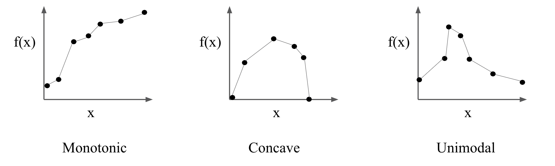
The most common and popular shape constraint is monotonicity. For a 1D function with , a function is monotonically increasing if is non-decreasing as increases, or monotonically decreasing if the opposite. Here we use the shorthand monotonic for either direction. For differentiable functions, a function is monotonic if the first derivative is non-negative everywhere. An example of a simple 1D monotonic function class is the set of linear functions with positive slopes.
A popular flexible 1D function class for satisfying shape constraints is piecewise linear functions (PLF) Barlow et al. 1972; Howard & Jebara 2008; Groeneboom & Jongbloed 2014; Garcia et al. 2012; Gupta et al. 2016, as shown in Figure 4.
Monotonicity constraints can also be applied to multi-dimensional functions with , where the usual definition is that is increasing in the th feature, , if is non-decreasing as increases, with all other features held fixed. A function can be monotonic with respect to a subset of its features. Flexible multi-dimensional monotonic functions have been created by constraining neural networks, (Archer & Wang 1993; Sill 1998; Zhang & Zhang 1999; Daniels & Velikova 2010; Minin et al. 2010; Qu & Hu 2011; Zhu et al. 2017; Cannon 2018; Wehenkel & Louppe 2019, e.g.,), support vector machines Howard & Jebara 2008, decision trees (Qian et al. 2015; Pei & Hu 2018, e.g.,), and lattices (Gupta et al. 2016; Canini et al. 2016; You et al. 2017, e.g.,), or by post-processing (Chernozhukov:2010; Bonakdarpour et al. 2018, e.g.,).
Other shape constraints that have been used for machine-learning include diminishing returns Pya & Wood 2015; Chen & Samworth 2016; Gupta et al. 2018, complementary inputs Gupta et al. 2020, and dominance between inputs Gupta et al. 2020.

Another overly-restrictive special case of unimodality is jointly concave functions. These have been produced by summing jointly concave basis functions Kim et al. 2004; Magnani & Boyd 2009, or by DNN’s with ReLU activations that are constrained to be jointly convex over a subset of features Dugas et al. 2009; Amos et al. 2017. We show experimentally that concave functions are generally too restrictive for finding and understanding global maximizers.
Shape constraints are often applied to lattice functions, as we do in this paper. Lattices are linearly-interpolated multidimensional look-up tables Garcia et al. 2012: in one-dimension a lattice is just a piecewise linear function with regular knots. Lattices are arbitrarily flexible, just add more knots (parameters). Because the lattice is parameterized by a regular grid of function values, many shape constraints turn into sparse linear inequality constraints, making training them easy Gupta:2016; Gupta et al. 2018; Gupta et al. 2020. Higher-dimensional lattice functions are achieved through ensembles Canini et al. 2016 and multi-layer models You et al. 2017; Cotter et al. 2019. In the next section, we will show how to construct efficient GONs using multi-layer lattice models with the appropriate shape constraints. Tensorflow Lattice provides an open source library for lattice functions Milani Fard 2020, we provide extensions to the Tensorflow Lattice library for GONs.
Appendix B Block Diagrams for Ensemble GON and CGON Models
Fig. 6 gives a block diagram for a DLN GON using an ensemble of lattices as a layer (for more on lattice ensembles see Canini et al. 2016, and for more on ensembles of lattices as a layer in a multi-layer model see You et al. 2017.
Fig. 7 gives a block diagram for a DLN CGON.
Appendix C Puzzles Experiment More Details
To further build intuition, in Figure 8 we show the trained functions with the most flexible hyperparameter choices we validated over. The most flexible GON model used keypoints for the PLF for each of the two inputs for , and then a lattice for . It has a steep peak at 213 pieces and year 2000. The most flexible DNN, with 4 layers and 8 hidden nodes, is a reasonable model with a peak at 353 pieces and art from year 2000. The GPR model with overfit good sales data for one of the largest puzzles. The most flexible ICNN model, with 4 layers and 8 hidden nodes, still advises the company to make puzzles with zero pieces.
 |
Appendix D Proofs
Below are the proofs for all of the results in the paper. See Fig. 9 for a Venn diagram summarizing Propositions 1,2,3 and 4.

D.1 Unimodal Functions Are GONs
See 3.2
Proof.
All unimodal functions are GONs. This is because for any unimodal function with maximizer , we can reparametrize it as for some that is unimodal with . This can then be written where is invertible, thus forming a GON. ∎
D.2 Concave Functions Are Unimodal
See 3.2
Proof.
Let , , be a ray in originating at . To prove concave is unimodal, we need to show that is decreasing. Let be two points on the ray with . Then it’s easily verified that . Now by the concavity of , we have
where the last inequality follows since is the maximum of . ∎
D.3 One-Dimensional GONs With Monotonic Are Unimodal
We show that for one-dimensional GONs because a continuous one-to-one function defined on a convex set must be monotonic, the GON is unimodal.
See 3.2
Proof.
Let be the pre-image of under . Consider any such that . Note that to be bijective, a continous one-dimensional with a convex domain must be either monotonically increasing or monotonically decreasing: otherwise, one can find 3 points for which either or and by the mean value theorem it follows that any point in between and will have at least 2 distinct pre-images, contradicting being one-to-one. Without loss of generality, assume is monotonically increasing. Then we have . Since is unimodal w.r.t its input , we have . Therefore is increasing for . An analogous argument shows that is decreasing for . Thus is unimodal with respect to . ∎
D.4 Proof for Linear Inequality Constraints To Make A Lattice Function Unimodal
Some visual intution for this lemma is given in Figure 5.
Throughout this section we use the following notation. For a function we denote its partial derivative with respect to the th input variable by . If is univariate we denote its derivative by . For we use to denote the set and for , and , we denote by the th entry of . Finally, we denote by the one-hot vector where iff .
Consider a lattice with dimension , size vector , and parameters . For , we define the cell of to be the set of its neighboring grid vertices given by . Then the lattice function is given by
| (11) |
where is the linear interpolation weight on vertex given by:
| (12) |
and is the standard indicator function. See Gupta et al. 2016 for more details.
To prove Lemma 1, we’ll need the following supporting lemma (Lemma 2), which gives a formula for the partial derivative of a lattice function.
Lemma 2: Let be a lattice function with dimension , size vector and parameters . Then for all , and with (i.e. does not lie on the boundary of two adjacent lattice cells in the th direction)
where is , if , or , otherwise, and .
Proof.
Let satisfy the requirements of the lemma. By (11), . Denoting by , for and , we get
where we used the fact that for , . Partitioning the set of size into the pairs , we may regroup the summands to obtain
| (13) |
Now, observe that . Thus, for with , it holds that
| (14) |
Substituting (D.4) into (13), we get
∎
We are now ready to prove Lemma 1.
See 4.4
Proof.
Every restriction obtained from by fixing the last features to constants is unimodal w.r.t if and only if every such restriction is decreasing along rays originating in . The latter statement can be equivalently restated as: for each , the function , given by , with , is decreasing. Since each such is continuous and piecewise-differentiable with finitely many pieces, the last condition is equivalent to requiring that for all where the derivative is defined. Observe that it’s sufficient to require that for all , , when it’s defined, since . Therefore, statement 1 of the lemma holds if and only if
| (15) |
By the chain rule, and hence using Lemma we have
where to get the last equality we added to and subtracted from each summand the quantity .
Next, for a fixed , partitioning the set of size into the pairs , we regroup the terms in the summation and get
| (16) | ||||
| (17) |
Now, using (12) and defining for and , we have for each , with
where to get the last equality, observe that for , the th entry of and is the same. Noting that and that , we get
| (18) |
Hence is a multi-linear interpolation of the values on . Thus requiring that it would be nonpositive for all is equivalent to requiring that
It’s easy to verify that these are precisely the inequalities in Statement 2. ∎
D.5 Unimodal Lattice Not Sufficient For a GON To Be Unimodal
See 4.6
Proof.
Our proof is by counterexample. Let be the function of the 2D lattice with size and vertex values: . It’s easy to verify that equation (8) of Lemma 1 holds for s=2. Thus satisfies the unimodality shape constraint with maximizer . Now, let and be the PLFs given by:
and
Let . Then it can be easily verified that the global maximizer of is at and it is unique. Thus for to satisfy the unimodal shape constraint, it must do so with maximizer . However is not decreasing along the ray , since and .
See Figure 10 for the illustration of the and functions.
 |
∎
D.6 Ensemble of Unimodal Functions is Unimodal
See 4.7
Proof.
Let , be a ray in originating in for some . We need to show that is decreasing for . Since , is a ray in in direction originating in , it follows by the unimodality of each that is decreasing for . The result now follows from the fact that a conical sum of decreasing functions is decreasing. ∎
Appendix E Details for Monarchs’ Reigns Experiments
We provide more details on the data and experimental results.
E.1 Data Details for Monarchs’ Reigns Experiments
The data can be downloaded at www.kaggle.com/senzhaogoogle/kingsreign.
All fifty dynasties were sampled from across the globe and from ancient to modern times. The original Monarchs’ Reigns dataset Feldman et al. 2014 (also known as Kings’ Reigns, but some of the monarchs were queens or had other titles) consists of 30 royal dynasties, for example the 36 monarchs of the Ottoman Empire from 1299-1922, the 15 monarchs of the Kings of Larsa from 1961 BC to 1674 BC, and the 4 monarchs of the Zulu Dynasty of 1816-1879. We added a test set of 20 additional royal dynasties using the same methodology used for the original dataset based on conversations with the original dataset creator Kyle Stewart (based on conversations about methodology). Example test set dynasties are the 5 monarchs of the 18th century Hotak dynasty in Afghanistan, and the 27 monarch Joseon dynasty of Korea that ended in 1910. All information came from Wikipedia. We will provide a Kaggle notebook for the complete train and test datasets.
The train and test datasets have the following known sampling biases:
- •
Dynasties for which there were more complete and well-organized records on Wikipedia were more likely to be sampled. This likely caused under-sampling of pre-Columbian American dynasties, for example.
- •
An effort was made to sample geographically diverse dynasties, which may have caused under-sampling of some regions and over-sampling of other regions with regards to population.
- •
An effort was made to sample dynasties across time, which may have caused under-sampling of some timeframes and over-sampling of others with regards to population.
- •
Current dynasties where the last monarch is still reigning were not sampled.
We note that our use of this data simplifies a number of potentially important factors about the stability of dynasties. For example, in monogamous cultures, it was more difficult to ensure a direct heir than in polygamous cultures Duindam 2015. A second issue is simply the definition of dynastic boundaries: what counts as a new dynasty, and has that criteria been sufficiently uniformly applied to the diverse dynasties in this dataset? A third issue is we treated the dynasties as though they were samples drawn IID from the same distribution, but the general reduction in violence over documented history Pinker 2011 might imply a shifting distribution towards more stable dynasties, given that many change-overs were due to violence.
E.2 Experimental Details for Monarchs’ Reigns
The train set had dynasties, and the test set had dynasties. For each method, we cross-validated over 18 choices of hyperparameters by leave-one-out cross-validation: we left out one-dynasty at a time and trained a model with each choice of hyperparameters on the other 29 dynasties. For each trained model and left-out dynasty, the predicted maximizer was computed as: , and we scored by the actual number of years reigned by that monarch in the left-out dynasty. Averaging those scores over the 30 rounds of one-dynasty-left-out formed the overall validation score for that hyperparameter choice. Tables in the Appendix list the 18 hyperparameter choices and corresponding validation scores for each method.
The test metric is the same as the cross-validation metric: for each trained model and each test dynasty, the predicted maximizer was computed as: , and we scored by the actual number of years reigned by that monarch in that test dynasty. Averaging those scores over the 20 test dynasties formed the overall test score for that method.
Table 7 shows that the GON model achieved the best test score, followed by the GPR. Note that while both DNN and GON predict a 6th monarch will rule longest, their test scores differ because they made different predictions for the maximizer for test dynasties that have fewer than 6 monarchs, as can be seen in Figure 1.
| Model | Train Set: | Test Set: Mean Actual | Global |
|---|---|---|---|
| Root MSE | Reign of Model’s Arg Max’s | Arg Max | |
| DNN | 14.67 | 15.05 | 6th monarch |
| FICNN | 14.89 | 14.75 | 1st monarch |
| GPR | 15.54 | 16.40 | 7th monarch |
| GON | 14.80 | 16.95 | 6th monarch |
E.3 Cross-Validation Scores For Different Hyperparameters
The complete cross-validation scores are shown for all the tried hyperparameters in Tables 8, 9 and 10.
| Model | Number Keypoints in | Number Keypoints in | Validation Score |
| GON | 3 | 2 | 21.23 |
| GON | 3 | 3 | 20.97 |
| GON | 3 | 5 | 25.30 |
| GON | 3 | 7 | 25.26 |
| GON | 3 | 9 | 26.00 |
| GON | 3 | 11 | 23.8 |
| GON | 5 | 2 | 22.97 |
| GON | 5 | 3 | 18.33 |
| GON | 5 | 5 | 25.27 |
| GON | 5 | 7 | 20.06 |
| GON | 5 | 9 | 22.80 |
| GON | 5 | 11 | 20.93 |
| GON | 7 | 2 | 22.47 |
| GON | 7 | 3 | 22.46 |
| GON | 7 | 5 | 18.33 |
| GON | 7 | 7 | 18.50 |
| GON | 7 | 9 | 20.77 |
| GON | 7 | 11 | 18.73 |
| GON | 9 | 2 | 22.46 |
| GON | 9 | 3 | 18.30 |
| GON | 9 | 5 | 19.73 |
| GON | 9 | 7 | 19.20 |
| GON | 9 | 9 | 21.13 |
| GON | 9 | 11 | 22.10 |
| Model | Number Layers | Number Hidden Nodes | Validation Score |
| FICNN | 3 | 2 | 22.47 |
| FICNN | 3 | 4 | 22.47 |
| FICNN | 3 | 8 | 22.20 |
| FICNN | 3 | 16 | 22.00 |
| FICNN | 3 | 32 | 21.20 |
| FICNN | 3 | 64 | 20.70 |
| FICNN | 4 | 2 | 22.93 |
| FICNN | 4 | 4 | 23.17 |
| FICNN | 4 | 8 | 21.83 |
| FICNN | 4 | 16 | 21.63 |
| FICNN | 4 | 32 | 21.20 |
| FICNN | 4 | 64 | 20.50 |
| FICNN | 5 | 2 | 20.36 |
| FICNN | 5 | 4 | 22.30 |
| FICNN | 5 | 8 | 20.70 |
| FICNN | 5 | 16 | 20.96 |
| FICNN | 5 | 32 | 19.40 |
| FICNN | 5 | 64 | 20.70 |
| FICNN | 6 | 2 | 22.06 |
| FICNN | 6 | 4 | 20.77 |
| FICNN | 6 | 8 | 21.83 |
| FICNN | 6 | 16 | 19.73 |
| FICNN | 6 | 32 | 21.50 |
| FICNN | 6 | 64 | 19.73 |
| Model | Number Layers | Number Hidden Nodes | Validation Score |
| DNN | 3 | 2 | 21.87 |
| DNN | 3 | 4 | 18.03 |
| DNN | 3 | 8 | 17.53 |
| DNN | 3 | 16 | 19.73 |
| DNN | 3 | 32 | 21.26 |
| DNN | 3 | 64 | 22.4 |
| DNN | 4 | 2 | 19.97 |
| DNN | 4 | 4 | 20.26 |
| DNN | 4 | 8 | 20.43 |
| DNN | 4 | 16 | 19.4 |
| DNN | 4 | 32 | 20.4 |
| DNN | 4 | 64 | 21.20 |
| DNN | 5 | 2 | 22.46 |
| DNN | 5 | 4 | 18.76 |
| DNN | 5 | 8 | 22.16 |
| DNN | 5 | 16 | 21.03 |
| DNN | 5 | 32 | 22.47 |
| DNN | 5 | 64 | 24.13 |
| DNN | 6 | 2 | 22.46 |
| DNN | 6 | 4 | 19.76 |
| DNN | 6 | 8 | 21.80 |
| DNN | 6 | 16 | 24.13 |
| DNN | 6 | 32 | 24.70 |
| DNN | 6 | 64 | 24.20 |
| Model | Validation Score | |
|---|---|---|
| GPR | 18.97 | |
| GPR | 17.83 | |
| GPR | 17.46 | |
| GPR | 16.83 | |
| GPR | 18.13 | |
| GPR | 20.7 | |
| GPR | 21.43 | |
| GPR | 21.6 | |
| GPR | 14.93 | |
| GPR | 18.97 | |
| GPR | 21.7 | |
| GPR | 22.47 | |
| GPR | 22.47 | |
| GPR | 22.47 | |
| GPR | 23.27 | |
| GPR | 19.63 | |
| GPR | 19.70 | |
| GPR | 19.70 | |
| GPR | 19.70 | |
| GPR | 19.70 | |
| GPR | 19.70 | |
| GPR | 19.70 | |
| GPR | 19.70 | |
| GPR | 19.70 |
Appendix F Details for Puzzles Experiments
The hyperparameter choices were designed to give a range of flexibility. For the FICNN and DNN models, choices were either or layers ( layers being the default in Amos et al. 2017), and either hidden nodes. The GPR hyperparameter was the sklearn standard covariance matrix additive smoothing parameter , ranging from to 10 in steps of 10. All GON models used a unimodal lattice layer for , and varied the number of keypoints in ’s PLFs from to . Because the first and last PLF keypoint are fixed to map to the lattice layer’s input domain, the case is equivalent to not having a first layer. Any ties were decided in favor of the hyperparameters corresponding to a more-regularized model.
Table 12 and 13 reports actual sales of the highest-predicted validation and test puzzles. The GON was most accurate in predicting the best-selling test puzzle, followed by the DNN and GON. The GPR model chose a test puzzle that was actually a terrible seller.
Our test metric was limited to the test set of puzzles for which there was 2019 sales numbers. In practice though, the business would like to use such a model for guidance as to which new puzzles they should create. For such use, we should ask if the global maximizer is reasonable. As seen in Figure 3, the FICNN and DNN models extrapolated poorly from a popular small puzzle in the train set, leading those models to predict that the global optimizer would be a jigsaw puzzle with zero pieces, which is not reasonable guidance. We questioned whether this was simply bad luck in selecting the hyperparameters, but in fact, 5 of the 8 FICNN models trained predicted the argmax at 0 pieces (see Table 12 in the Appendix). The DNN also only gave reasonable answers for the global maximizer for 3 of its 8 hyperparameter choices.
The five most-flexible GON models consistently predicted a global optimizer would be a puzzle with 190-230 pieces and artwork from around the year 2000. Partners at Artifact said that based on their ten years of sales experience, such puzzles do tend to sell best.
We also note the GON models also generally predicted the best year for art was 2000, which is at the edge of the input domain, which confirms the proposed unimodal shape constraints do not block fitting models with their maximizer on the edge of the input domain.
| Model | Actual Sales of | Actual Sales of | Global Arg Max |
| Highest-Scored | Highest-Scored | ||
| Validation Puzzle | Test Puzzle | ||
| DNN 3 layers, 2 hid. | flat model | – | – |
| DNN 3 layers, 4 hid. | 21 | 30 | 1200 pieces, year 2000 |
| DNN 3 layers, 6 hid. | 74 | 182 | 192 pieces, year 2000 |
| DNN 3 layers, 8 hid. | 88 | 173 | 0 pieces, year 2000 |
| DNN 4 layers, 2 hid. | flat model | – | – |
| DNN 4 layers, 4 hid. | 0 | 7 | 0 pieces, year 1500 |
| DNN 4 layers, 6 hid. | 10 | 30 | 192 pieces, year 2000 |
| DNN 4 layers, 8 hid. | 16 | 164 | 353 pieces, year 2000 |
| FICNN 3 layers, 2 hid. | 43 | 173 | 0 pieces, year 2000 |
| FICNN 3 layers, 4 hid. | 88 | 173 | 0 pieces, year 2000 |
| FICNN 3 layers, 6 hid. | 88 | 173 | 0 pieces, year 2000 |
| FICNN 3 layers, 8 hid. | 74 | 182 | 192 pieces, year 2000 |
| FICNN 4 layers, 2 hid. | 88 | 173 | 0 pieces, year 2000 |
| FICNN 4 layers, 4 hid. | 74 | 13 | 0 pieces, year 2000 |
| FICNN 4 layers, 6 hid. | 74 | 182 | 0 pieces, year 2000 |
| FICNN 4 layers, 8 hid. | 88 | 173 | 0 pieces, year 2000 |
| Model | Actual Sales of | Actual Sales of | Global Arg Max |
|---|---|---|---|
| Highest-Scored | Highest-Scored | ||
| Validation Puzzle | Test Puzzle | ||
| GPR | 21 | 3 | 168 pieces, year 1500 |
| GPR | 21 | 182 | 242 pieces, year 2000 |
| GPR | 74 | 182 | 242 pieces, year 2000 |
| GPR | 74 | 182 | 242 pieces, year 2000 |
| GPR | 88 | 173 | 68 pieces, year 2000 |
| GPR | 43 | 173 | 68 pieces, year 2000 |
| GPR | 43 | 173 | 68 pieces, year 2000 |
| GPR | 88 | 2 | 146 pieces, year 2000 |
| GON 2kp | 43 | 1 | 600 pieces, year 1700 |
| GON 3kp | 31 | 21 | 502 pieces, year 1400 |
| GON 4kp | 76 | 182 | 230 pieces, year 2000 |
| GON 5kp | 74 | 182 | 190 pieces, year 2000 |
| GON 6kp | 13 | 182 | 212 pieces, year 2000 |
| GON 7kp | 74 | 182 | 191 pieces, year 2000 |
| GON 8kp | 74 | 182 | 194 pieces, year 2000 |
| GON 9kp | 74 | 182 | 213 pieces, year 2000 |
Appendix G Details for Wine Experiments
Figure 11 shows the results for the experiments conditioned on price.
 |
| Model | Val | Train | Test | Test Maximizer |
|---|---|---|---|---|
| Score | MSE | Score | ||
| DNN: 2 layers, 2 nodes | 97 | 2.54 | 88 | $3300, acid, juicy, tannin, France |
| DNN: 2 layers, 4 nodes | 97 | 2.53 | 88 | $3300, acid, juicy, tannin, France |
| DNN: 2 layers, 8 nodes | 97 | 2.54 | 88 | $3300, acid, juicy, tannin, France |
| DNN: 2 layers, 16 nodes | 97 | 2.47 | 88 | $3300, acid, juicy, tannin, France |
| DNN: 2 layers, 32 nodes | 97 | 2.30 | 88 | $3300, acid, juicy, tannin, France |
| DNN: 2 layers, 64 nodes | 92 | 2.24 | 94 | $1100, complex, earth, lees, tight, Austria |
| DNN: 3 layers, 2 nodes | 97 | 2.55 | 88 | $3300, acid, juicy, tannin, France |
| DNN: 3 layers, 4 nodes | 97 | 2.55 | 88 | $3300, acid, juicy, tannin, France |
| DNN: 3 layers, 8 nodes | 97 | 2.55 | 88 | $3300, acid, juicy, tannin, France |
| DNN: 3 layers, 16 nodes | 97 | 2.27 | 88 | $3300, acid, juicy, tannin, France |
| DNN: 3 layers, 32 nodes | 97 | 2.23 | 88 | $3300, acid, juicy, tannin, France |
| DNN: 3 layers, 64 nodes | 97 | 2.24 | 88 | $3300, acid, juicy, tannin, France |
| DNN: 4 layers, 2 nodes | 97 | 2.54 | 88 | $3300, acid, juicy, tannin, France |
| DNN: 4 layers, 4 nodes | 97 | 2.53 | 88 | $3300, acid, juicy, tannin, France |
| DNN: 4 layers, 8 nodes | 97 | 2.27 | 88 | $3300, acid, juicy, tannin, France |
| DNN: 4 layers, 16 nodes | 97 | 2.23 | 88 | $3300, acid, juicy, tannin, France |
| DNN: 4 layers, 32 nodes | 97 | 2.23 | 88 | $3300, acid, juicy, tannin, France |
| DNN: 4 layers, 64 nodes | 97 | 2.17 | 88 | $3300, acid, juicy, tannin, France |
| Model | Val | Train | Test | Test Maximizer |
|---|---|---|---|---|
| Score | MSE | Score | ||
| FICNN: 2 layers, 2 nodes | 97 | 2.52 | 88 | $3300, acid, juicy, tannin, France |
| FICNN: 2 layers, 4 nodes | 97 | 2.29 | 88 | $3300, acid, juicy, tannin, France |
| FICNN: 2 layers, 8 nodes | 91 | 2.33 | 95 | $412, jam, opulent, France |
| FICNN: 2 layers, 16 nodes | 92 | 2.27 | 100 | $848, acid, hint of, opulent, toast, France |
| FICNN: 2 layers, 32 nodes | 98 | 2.20 | 94 | $1100, complex, earth, lees, tight, Austria |
| FICNN: 2 layers, 64 nodes | 96 | 2.19 | 94 | $1100, complex, earth, lees, tight, Austria |
| FICNN: 3 layers, 2 nodes | 97 | 2.53 | 88 | $3300, acid, juicy, tannin, France |
| FICNN: 3 layers, 4 nodes | 96 | 2.30 | 94 | $1100, complex, earth, lees, tight, Austria |
| FICNN: 3 layers, 8 nodes | 96 | 2.25 | 94 | $1100, complex, earth, lees, tight, Austria |
| FICNN: 3 layers, 16 nodes | 96 | 2.23 | 94 | $1100, complex, earth, lees, tight, Austria |
| FICNN: 3 layers, 32 nodes | 91 | 2.24 | 96 | $351 oak, tannin, tight, toast, Spain |
| FICNN: 3 layers, 64 nodes | 92 | 2.30 | 94 | $1100, complex, earth, lees, tight, Austria |
| FICNN: 4 layers, 2 nodes | 97 | 2.40 | 94 | $1100, complex, earth, lees, tight, Austria |
| FICNN: 4 layers, 4 nodes | 97 | 2.24 | 94 | $900, elegant, Italy |
| FICNN: 4 layers, 8 nodes | 97 | 2.26 | 85 | $320, acid, crisp, Romania |
| FICNN: 4 layers, 16 nodes | 97 | 2.28 | 88 | $3300, acid, juicy, tannin, France |
| FICNN: 4 layers, 32 nodes | 97 | 2.47 | 88 | $3300, acid, juicy, tannin, France |
| FICNN: 4 layers, 64 nodes | 97 | 2.47 | 88 | $3300, acid, juicy, tannin, France |
| Model | Val | Train | Test | Test Maximizer |
|---|---|---|---|---|
| Score | MSE | Score | ||
| GON 100 2D lattices, 5kp | 92 | 2.31 | 95 | $100 acid, cassis, complex, refined |
| structure, tannin, velvet, US | ||||
| GON 100 2D lattices, 9kp | 93 | 2.29 | 97 | $375, acid, bright, complex, elegant, |
| refined, structure, tannin, Italy | ||||
| GON 100 2D lattices, 13kp | 93 | 2.31 | 97 | $375, acid, bright, complex, elegant |
| refined, structure, tannin, Italy | ||||
| GON 200 2D lattices, 5kp | 97 | 2.30 | 97 | $165 acid, cassis, complex, mineral |
| oak, refined, structure, tannin, US | ||||
| GON 200 2D lattices, 9kp | 98 | 2.28 | 97 | $375, acid, bright, complex, elegant |
| refined, structure, tannin, Italy | ||||
| GON 200 2D lattices, 13kp | 98 | 2.26 | 97 | $375, acid, bright, complex, elegant |
| refined, structure, tannin, Italy | ||||
| GON 400 2D lattices, 5kp | 96 | 2.32 | 95 | $100, acid, cassis, complex |
| refined, structure, tannin, velvet, US | ||||
| GON 400 2D lattices, 9kp | 97 | 2.27 | 97 | $375, acid, bright, complex, elegant |
| refined, structure, tannin, Italy | ||||
| GON 400 2D lattices, 13kp | 97 | 2.25 | 94 | $1100, complex, earth, lees |
| tight, Austria | ||||
| GON 800 2D lattices, 5kp | 97 | 2.28 | 97 | $375, acid, bright, complex, elegant |
| refined, structure, tannin, Italy | ||||
| GON 800 2D lattices, 9kp | 98 | 2.26 | 94 | $1100, complex, earth, lees |
| tight, Austria | ||||
| GON 800 2D lattices, 13kp | 93 | 2.24 | 97 | $375, acid, bright, complex, elegant |
| refined, structure, tannin, Italy | ||||
| GON 1600 2D lattices, 5kp | 97 | 2.26 | 96 | $180 butter, complex, lees, |
| mineral US | ||||
| GON 1600 2D lattices, 9kp | 97 | 2.37 | 94 | $1100, complex, earth, lees |
| tight, Austria | ||||
| GON 1600 2D lattices, 13kp | 94 | 2.22 | 96 | $450, cream, dense, mineral |
| tight, France |
Appendix H Details for Hyperparameter Optimization for Image Classifiers
As mentioned in the main paper, image classifers shown in the main paper are trained for epochs. We use ADAM with the default learning rate of 0.001 with a batch size of 128 to train the classifiers.
For GON and CGON, we use an ensemble of unimodal lattices. All methods are trained for 250 epochs.
Hyperparameters for the optimizers are validated based on 5-fold MSE, which are summarized in Table 17 below.
| Global Optimization | Conditional Global Optimization | |||||||
|---|---|---|---|---|---|---|---|---|
| Rosenbrock | GON | FICNN | DNN | GPR | CGON | PICNN | DNN | GPR |
| PLF kps per input | 5 | - | - | - | 5 | - | - | - |
| Lattice kps per input | 3 | - | - | - | 3 | - | - | - |
| Inputs each lattice fuses | 2 | - | - | - | 2 | - | - | - |
| Num hidden layers | - | 1 | 1 | - | - | 1 | 1 | - |
| Num hidden nodes | - | 256 | 32 | - | - | 32 | 32 | - |
| in GPR | - | - | - | 0.01 | - | - | - | 0.01 |
Appendix I Details for Simulations with Standard Global Optimization Functions
We ran simulations on two standard benchmark functions, the banana-shaped Rosenbrock function, and the pocked-convex Griewank function, to compare GON against FICNN, DNN, GPR and sample best. For conditional global optimization problems, we compared CGON against PICNN, DNN and GPR.
The multi-dimensional Rosenbrock function has the formula:
| (19) |
The multi-dimensional Griewank function has the formula:
| (20) |
See Figure 12 for a visulization of 2-dimensional Rosenbrock and Griewank functions. For both functions, the true global minimizer is at .
| Rosenbrock | Griewank |
For each function, we randomly generated 50 training sets for each of 60 different experimental set-ups: inputs training examples noise levels where the training label is for . For the conditional global optimization problem, we aim to find , where is the first inputs and is the last inputs. Once FICNN/PICNN fit their convex/conditionally-convex functions, their minimizers are found using ADAM with learning rate .001 and 10k steps with projections onto the input domain . Details on hyperparameter validation for all methods are in the Appendix.
We found the global maximizer of each response surface as in experiment in Section 5.5. That is, for GON and CGON, we found the global maximizer of the response surface by inverting the PLFs. For FICNN and PICNN, we used ADAM to find their global maximizers. For DNN and GPR, we first generated a finite random set of 100,000 inputs across the domain of and set .
Table 18 shows that GON is consistently the best method for all twelve different simulation set-ups. CGON is also consistently best for Rosenbrock. For the globally convex Griewank, CGON is the best or tied for the best in 6 slices, whereas PICNN, DNN and GPR are the best or tied for the best in 0, 5 and 3 slices, respectively. GON and CGON performed especially well in the more challenging cases of large and high noise and few training samples .
Note that the performance of sample best deteriorates with more training samples, as there is more risk it will overfit a particularly noisy training sample. In fact, in general the performance of the different response surface methods did not necessarily get better with more training samples , which we suspect is due to the fact that as increases, there is a greater chance of more very noisy samples that confuses the response surface placement of its maximizer.
| Global Optimization | Conditional Global Optimization | ||||||||
| Rosenbrock | GON | FICNN | DNN | GPR | Sample Best | CGON | PICNN | DNN | GPR |
| 213 24 | 833 92 | 2259 151 | 2310 186 | 3271 156 | 903 68 | 1473 132 | 1769 136 | 1558 157 | |
| 492 37 | 2370 188 | 5019 209 | 4791 241 | 5463 237 | 1340 76 | 5799 283 | 4334 201 | 3822 226 | |
| 734 47 | 3575 278 | 7407 220 | 7022 257 | 7559 273 | 1762 86 | 10650 401 | 6475 213 | 5430 256 | |
| 1004 21 | 5750 128 | 9466 91 | 9133 107 | 9571 113 | 2164 36 | 15682 177 | 8085 82 | 7855 91 | |
| 282 8 | 818 34 | 4064 110 | 6582 201 | 1576 59 | 943 22 | 5478 178 | 3269 102 | 5054 165 | |
| 419 13 | 1273 52 | 5183 116 | 3830 117 | 6102 97 | 1093 23 | 6825 193 | 4260 101 | 3763 126 | |
| 557 16 | 2805 97 | 6216 113 | 5737 95 | 7685 102 | 1500 32 | 8622 205 | 5405 104 | 3772 96 | |
| 797 22 | 4382 118 | 7075 105 | 6445 77 | 8385 108 | 1986 40 | 10151 217 | 6184 98 | 5143 76 | |
| 999 26 | 6383 139 | 7651 105 | 6478 70 | 8583 109 | 2188 44 | 10929 217 | 6710 91 | 5599 65 | |
| 473 9 | 2983 78 | 6462 83 | 5820 90 | 5042 80 | 1583 30 | 11407 173 | 5736 74 | 5077 80 | |
| 897 19 | 4281 104 | 6237 87 | 5923 97 | 6481 93 | 1665 29 | 8451 152 | 5196 77 | 4777 87 | |
| 463 13 | 2133 71 | 5414 97 | 5700 103 | 7875 101 | 1379 25 | 5345 133 | 4564 91 | 4145 95 | |
| Griewank | GON | FICNN | DNN | GPR | Sample Best | CGON | PICNN | DNN | GPR |
| 0.45 0.007 | 0.49 0.009 | 0.82 0.012 | 0.71 0.014 | 1.12 0.015 | 0.81 0.007 | 0.79 0.010 | 0.79 0.012 | 0.70 0.013 | |
| 0.51 0.006 | 0.83 0.006 | 0.91 0.007 | 0.99 0.007 | 1.03 0.008 | 0.93 0.004 | 0.96 0.004 | 0.91 0.006 | 0.94 0.008 | |
| 0.59 0.005 | 0.90 0.004 | 0.97 0.004 | 1.02 0.002 | 1.04 0.004 | 0.97 0.003 | 1.00 0.002 | 0.96 0.004 | 1.01 0.003 | |
| 0.64 0.005 | 0.94 0.003 | 1.00 0.002 | 1.01 0.002 | 1.02 0.003 | 0.97 0.002 | 1.01 0.001 | 0.99 0.003 | 1.01 0.002 | |
| 0.53 0.006 | 0.65 0.008 | 0.73 0.010 | 0.74 0.012 | 0.68 0.012 | 0.87 0.005 | 0.86 0.008 | 0.72 0.010 | 0.76 0.011 | |
| 0.52 0.006 | 0.71 0.008 | 0.86 0.009 | 0.80 0.011 | 1.07 0.006 | 0.91 0.005 | 0.91 0.007 | 0.86 0.008 | 0.78 0.010 | |
| 0.52 0.006 | 0.79 0.008 | 0.95 0.007 | 0.95 0.009 | 1.13 0.007 | 0.93 0.005 | 0.95 0.006 | 0.93 0.007 | 0.92 0.009 | |
| 0.58 0.008 | 0.86 0.008 | 1.03 0.005 | 1.06 0.006 | 1.17 0.008 | 0.94 0.005 | 0.98 0.006 | 1.00 0.006 | 1.03 0.007 | |
| 0.60 0.008 | 0.93 0.007 | 1.05 0.005 | 1.10 0.006 | 1.19 0.008 | 0.95 0.006 | 1.00 0.005 | 1.05 0.006 | 1.09 0.006 | |
| 0.59 0.006 | 0.91 0.006 | 0.99 0.004 | 1.00 0.005 | 0.98 0.006 | 0.95 0.005 | 0.98 0.004 | 0.98 0.004 | 0.99 0.005 | |
| 0.52 0.005 | 0.79 0.007 | 0.98 0.005 | 0.94 0.008 | 1.04 0.008 | 0.91 0.004 | 0.97 0.005 | 0.97 0.006 | 0.92 0.007 | |
| 0.53 0.004 | 0.66 0.006 | 0.81 0.008 | 0.85 0.010 | 1.13 0.008 | 0.90 0.004 | 0.87 0.006 | 0.79 0.008 | 0.84 0.009 | |
The multi-dimensional Rosenbrock function has formula:
| (21) |
The multi-dimensional Griewank function has formula:
| (22) |
For both functions, the true global minimizer is at .
For both GON and CGON, we first use D PLFs with keypoints to calibrate the D inputs for optimization. The unimodal function consists of an enesemble of unimodal lattices, each fuses 3 inputs with keypoints. For CGON, we let be , where and denote the -th entry of and .
For FICNN and PICNN, we use the formulations in (2) (Figure 1) and (3) (Figure 2), respectively, in Amos, et al. Amos et al. 2017. All the hidden layers are constructed to have the same hidden dimensions, whenever possible. For DNN, we use fully connected hidden layers with a constant number of hidden nodes across layers. The number of hidden layers and the number of hidden nodes are treated as hyperparameters.
For GPR, we use RBF kernel with , which is the default in the sklearn package. The White Kernel is treated as a hyperparameter.
For each of the Rosenbrock and Griewank functions, we used grid search to choose hyperparameters for each method that minimize the average over the runs for each function ( repetitions with random seeds), where denotes the ground truth function. After choosing hyperparameters, we reran the simulation with 50 repetitions, and report the average-50 result in Table 5.6. The hyperprameters of each method are summarized in Table 19.
| Global Optimization | Conditional Global Optimization | |||||||
|---|---|---|---|---|---|---|---|---|
| Rosenbrock | GON | FICNN | DNN | GPR | CGON | PICNN | DNN | GPR |
| PLF kps per input | 10 | - | - | - | 10 | - | - | - |
| Lattice kps per input | 3 | - | - | - | 3 | - | - | - |
| Num hidden layers | - | 2 | 2 | - | - | 2 | 2 | - |
| Num hidden nodes | - | 16 | 32 | - | - | 16 | 16 | - |
| in GPR | - | - | - | 1.0 | - | - | - | 1.0 |
| Griewank | GON | FICNN | DNN | GPR | CGON | PICNN | DNN | GPR |
| PLF kps per input | 10 | - | - | - | 10 | - | - | - |
| Lattice kps per input | 3 | - | - | - | 3 | - | - | - |
| Num hidden layers | - | 4 | 2 | - | - | 2 | 2 | - |
| Num hidden nodes | - | 32 | 16 | - | - | 16 | 16 | - |
| in GPR | - | - | - | 1.0 | - | - | - | 1.0 |
Appendix J Open Questions
We defined GONs (and CGONs) by the shape constraints they must obey: a composition of invertible layers and unimodal layers. We showed how to construct such models using the piece-wise linear functions and lattice layers of DLNs, which are arbitrarily flexible models that are particularly amenable to shape constraints (Gupta et al. 2020; Cotter et al. 2019), but other functions could be used for the invertible layers Behrmann et al. 2019, and one could use convex networks for the needed unimodal layers (at the cost of some flexibility) (Amos et al. 2017).
Another open question is the choice of loss function when training GONs or other flexible response surfaces. In our experiments, all models were fit using standard mean-squared error. Since the goal of fitting the GON is to predict the maximizer only, it seems intuitive that one should worry more about fitting the examples closer to the (unknown) maximizer. We experimented with loss functions that up-weighted training examples with bigger label values, but, perhaps due to the flexibility of the GONs, did not find they helped much, and eschewed their extra complexity and hyperparameters.
We focused here on the setting where one makes only one prediction. However GONs could also be used as a response surface function within a global optimization algorithm that is able to make a series of guesses. In such a context it might make sense to evolve the neighborhood fit by the GON, or fit many GONs in parallel to different evolving neighborhoods for a multi-agent search like particle-swarm optimization Kennedy & Eberhart 1995; Shi & Eberhart 1998.
Lastly, this work is part of a recent wave of research into shape constraints showing that shape constraints can provide sensible regularization while not hurting useful expressability of AI models (e.g. Pya & Wood 2015; Chen & Samworth 2016; Gupta et al. 2016; Cannon 2018; Chetverikov et al. 2018; Cotter et al. 2019; Wehenkel & Louppe 2019; Gasthaus et al. 2019; Wang & Gupta 2020). We hope this work will inspire other useful shape constraint regularization strategies for AI.