Tracing stars in Milky Way satellites with A-SLOTHTracing stars in Milky Way satellites with A-SLOTH–D

a-sloth uses dark matter halo merger trees drawn from the lx14 run of the Caterpillar project (Griffen et al. 2016), which is a dark-matter-only cosmological simulation suite focusing on the assembly of MW-sized haloes and their satellite galaxies. The dark matter particles in the lx14 run have masses of $\sim 3\times 10^{4}{M}_{\odot}$ and the gravitational softening length is $76h^{-1}$pc. It is based on the Planck Collaboration et al. 2014 cosmological parameters in a 100 $h^{-1}$Mpc box. MW-like systems are selected at $z=0$ if the main haloes fulfill the following criteria:

1. 1.

   Virial mass in range $0.7\times 10^{12}{M}_{\odot}$ $\leq M_{\rm vir,peak}\leq 3\times 10^{12}{M}_{\odot}$.

2. 2.

   There is no halo with $M_{\rm vir,peak}\geq 7\times 10^{13}{M}_{\odot}$ within 7 Mpc.

3. 3.

   There are no other haloes with $M_{\rm vir,peak}\geq 0.5\times M_{\rm main}$ within 2.8 Mpc of the main halo.

Dark matter haloes are identified with rockstar (Behroozi et al. 2013) and $M_{\rm vir,peak}$ is the maximum virial mass along the main branch a halo ever attains up to the current redshift, that is computed with the evolution of the virial relation from Bryan & Norman 1998. We adopt their notation here. Griffen et al. 2016 extracted the full merger history of these MW-like systems, including dark matter and spatial information of the haloes and global time-steps between the snapshots, $\Delta t_{z}$, which is $\approx 5$Myr down to $z=6$ and $\approx 50$Myr at $z=6-0$. We have verified in an earlier study that the mass resolution of these merger trees is sufficient to model Pop III star formation at high redshift and using higher resolution merger trees yields converged results (see Appendix A of Magg et al. 2018). In this work, we select 30 merger trees from their sample. a-sloth walks through these merger trees and determines the baryonic contents of each halo in the merger tree based on the implemented physics. We describe the physical processes in the following sections.

We follow the same metal-free (Pop III) star formation (SF) model as in our previous works (Magg et al. 2018; Tarumi et al. 2020). We briefly summarize the model here. Pop III stars are assumed to form when H₂ can cool primordial gas efficiently, which means that a halo needs to exceed a critical mass, $M_{\rm crit}$. In a-sloth, Pop III stars form instantly in a single star burst in a mini-halo (haloes below the atomic cooling threshold ($T_{\rm vir}=10000\,\mathrm{K}$) as soon as its virial mass exceeds $M_{\rm crit}$. By default, we follow the prescriptions given in Schauer et al. 2021 and Hummel et al. 2012 to determine $M_{\rm crit}$. Schauer et al. 2021 showed that the critical mass is dependent on the LW background and the large-scale streaming velocity of the baryons relative to the dark matter:

Here, $M_{\rm crit,S21}$ is the critical mass in units of solar masses, $J_{21}$ is the strength of LW background in units of $10^{-21}\>{\rm erg\,s^{-1}\,cm^{-2}\,Hz^{-1}\,sr^{-1}}$, $v_{\rm BC}$ is the large-scale streaming velocity of the baryons relative to the dark matter in units of $\sigma_{\rm rms}$, and $\sigma_{\rm rms}$ is the root-mean-squared value of the streaming velocity. We denote this default model hereafter as S21. We do not self-consistently follow the build-up of the LW background, because the effective volume of our MW-like merger trees is too small to obtain a cosmologically representative estimate of the LW background. Instead, we adopt the simple redshift-dependent fitting formula,

which is based on the work in Greif & Bromm 2006. We take $v_{\rm BC}=0.8\sigma_{\rm rms}$ as the fiducial baryonic streaming velocity, since this is the most likely value to be present at a randomly selected point in the Universe (Schauer et al. 2021). The impact of varying our treatment of both of these effects is explored in Section 4.2.

In addition, we assume that gas can cool down efficiently and form stars in haloes that have virial temperatures above the atomic cooling limit ($T_{\rm vir}\geq 10^{4}{\rm K}$) when there is no strong ionizing radiation field (Visbal et al. 2017). Therefore, we consider haloes that have virial masses larger than $M_{\rm crit,10^{4}{\rm K}}$ can form Pop III stars, where $M_{\rm crit,10^{4}{\rm K}}$ is computed by

The final critical mass is then determined by $M_{\rm crit,fin}={\rm MIN}(M_{\rm crit,S21},M_{\rm crit,10^{4}{\rm K}})$.

Cold gas is converted to Pop III stars in haloes with $M_{\rm halo}\geq M_{\rm crit}$ at a fixed efficiency $\eta_{\rm III}$, defined such that $M_{{\rm*,III}}=\eta_{\rm III}\Omega_{\rm b}M_{\rm halo}/\Omega_{\rm m}$, where $M_{\rm halo}$ is the current virial mass of the halo, $\Omega_{\rm b}$ is the baryon density parameter today, and $\Omega_{\rm m}$ is the matter density parameter today. We adopt $\Omega_{\rm b}=0.0486$ and $\Omega_{\rm m}=0.3089$ (Planck Collaboration et al. 2016). We follow the Pop III model in Tarumi et al. 2020 and sample stars stochastically from an IMF with a slope of $dN/d(\rm{log}M)\propto M^{0.5}$ in the mass range of $2<M_{\rm*}<180{M}_{\odot}$. Further SF is halted when the total mass of newly-formed Pop III reaches $M_{\rm{*,III}}$.

We calculate the stellar lifetimes of Pop III stars by interpolating between values assembled from several previous studies: Marigo et al. 2001 for stars in the mass range 0.7-100${M}_{\odot}$; Schaerer 2002 for stars in the mass range 5-500${M}_{\odot}$ (and note that we consider their models without mass loss); and Ekström et al. 2008 for stars in the mass range 9-200${M}_{\odot}$. If the stellar lifetime of a star is provided by multiple works, we use the mean value. Pop III stars die as core-collapse supernovae (CCSNe) in the range of 10-40${M}_{\odot}$ and as pair-instability supernovae (PISNe) in the range of 140-260${M}_{\odot}$ (Heger & Woosley 2002; Heger & Woosley 2010). Following Tarumi et al. 2020, we further assume that $30\%$ ($f_{\rm faint}=0.3$) of the Pop III CCSNe explode as faint supernovae. We use the tabulated metal yields provided in Kobayashi et al. 2011 and Nomoto et al. 2013 for PISNe and normal CCSNe, and the yields in Ishigaki et al. 2014; Ishigaki et al. 2018 for faint CCSNe. We assume that a fraction $f_{\rm fallback}=0.2$ (Ritter et al. 2015) of the metals remains in the mini-halo after the supernovae have exploded, with the remaining fraction $(1-f_{\rm fallback})$ gaining enough energy from the SNe to escape from the gravitational well of the mini-halo. Tarumi et al. 2020 calibrated the Pop III SF efficiency ($\eta_{\rm III}$), $f_{\rm faint}$ and $f_{\rm fallback}$ to reproduce the observed MW metallicity distribution function (MDF). The main focus of this work is on the stellar masses of the dwarf galaxies and our model does not heavily depend on metallicity. Therefore, we adopt the same values of $\eta_{\rm III}$, $f_{\rm faint}$ and $f_{\rm fallback}$ as in Tarumi et al. 2020 without investigating the effects of these parameters in detail.

Following the initial Pop III star burst, we assume that any future star formation in the same halo will be in the form of metal-enriched stars. However, stellar feedback will have heated the gas in the mini-halo and ejected a fraction of it. Therefore, further SF is suppressed until the gas re-accumulates and cools down. We denote this time between the Pop III star burst and the onset of further star formation as $t_{\rm rec}$, known as the recovery time, which was calibrated by Tarumi et al. 2020.

In our model, we do not distinguish between metal-rich (Population I) and metal-poor (Population II) stars and classify all metal-enriched stars as Population II (Pop II) stars. We implement an improved Pop II SF model, which is based on the models in Magg et al. 2018 and Tarumi et al. 2020. The explanations of important variables in the Pop II SF model are listed in Table 1. We assume that the baryons initially associated with a given dark matter halo are located either in cold gas ($M_{\rm cold}$), in hot gas ($M_{\rm hot}$), in a Pop II stellar component ($M_{\rm*,II}$), or have been lost from the halo in an outflow ($M_{\rm out}$). The initial baryonic mass of a halo with virial mass $M_{\rm vir,peak}$ is assumed to be $(\Omega_{\rm b}/\Omega_{\rm m})M_{\rm vir,peak}$. Therefore, by construction

is always maintained in the model. Note that in our model, hot gas is any gas that is not cold, i.e. it corresponds to the sum of the warm and hot phases of the ISM in the usual three-phase description (Cowie et al. 1981; Klessen & Glover 2016). We do not account for Pop III stars in the mass budget because the small value we adopt for $\eta_{\rm III}$ means that they never represent more than a small fraction of they baryonic mass in any halo. Additionally, they occupy a negligible fraction of the stellar mass at $z=0$ and the Pop III stars that remain on the main sequence after $t_{\rm rec}$ are too low mass to contribute significantly to the stellar feedback.

Unlike Pop III SF, we assume that Pop II stars can form in multiple epochs, and so we further divide the global time-steps ($\Delta t_{z}$) from the merger tree into smaller ones. In other words, we have subcycles in our Pop II SF model. The subcycle time-step is denoted as $\delta t_{i}$, and we describe how we determine it in our simulation at the end of this section. A halo is labeled to trigger Pop II SF if the time since it experienced Pop III SF equals or exceeds $t_{\rm rec}$ or if it is externally enriched by supernovae from nearby haloes. Prior to the subcycling of Pop II SF, we initialize the halo by inheriting the baryonic contents from all of its progenitors, which gives us $M^{0}_{\rm cold}$, $M^{0}_{\rm hot}$, $M^{0}_{\rm*,II}$, and $M^{0}_{\rm out}$. Then, in time-step $i$ of the subcycle, the baryonic quantities are updated with the following equations:

We start from $i=0$ and make sure the last time-step in the subcycle always ends exactly at the next global time-step of the merger trees.

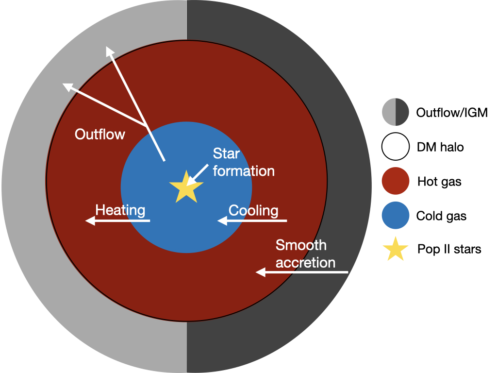
There are several physical processes that enter the above equations. We show the connections between these processes and the baryonic contents in our Pop II SF model in Figure 1:

1. 1.

   Cooling of hot gas

   We assume that hot gas cools on a timescale equal to the dynamical time of the stellar disk, $t_{\rm dyn}$. Therefore, during the subcycle time-step $\delta t_{i}$, a mass of gas $M^{i}_{\rm hot}\delta t_{i}/{t_{\rm dyn}}$ is transferred from the hot gas reservoir to the cold gas reservoir. We assume that cold gas and stars reside in a central region of the halo with a radius of $R_{s}$, where $R_{\mathrm{s}}=R_{\mathrm{vir}}/c_{\mathrm{dm}}$ and $c_{\mathrm{dm}}$ is the halo’s concentration. We follow the fitting functions of $c_{\mathrm{dm}}$ in Correa et al. 2015, which are also provided here in Appendix B.2. The dynamical time scale of the central region of the halo is computed with $t_{\mathrm{dyn}}=R_{\mathrm{s}}/v_{\mathrm{dyn}}$ and that the velocity is computed with $v_{\mathrm{dyn}}=\sqrt{G(M_{*}+M_{\mathrm{cold}})/R_{\mathrm{s}}}$.
   

2. 2.

   Heating of cold gas and gas removal by photoionization

   We consider the effects of photoionization feedback from massive stars, $\delta M^{i}_{\rm heat}$. In haloes below the atomic cooling limit ($T_{\rm vir}=10000$K), $\delta M^{i}_{\rm heat}$ is added directly to the outflow, whereas in haloes above the atomic cooling limit, an amount of gas with a mass of $\delta M^{i}_{\rm heat}$ is removed from the cold gas reservoir and added to the hot gas reservoir. The derivation of $\delta M^{i}_{\rm heat}$ is given in Section 2.4.
   

3. 3.

   Accretion of hot gas

   We assume that hot gas is continuously accreted from the intergalactic medium. In time-step $i$, an amount of hot gas

   		$\displaystyle\delta M^{i}_{{\rm acc,hot}}=$		(6)
   		$\displaystyle\left(\frac{\Omega_{\rm b}}{\Omega_{\rm m}}M_{\rm vir,peak}-M^{0}_{\rm cold}-M^{0}_{\rm hot}-M^{0}_{\rm*,II}-M^{0}_{\rm out}\right)\frac{\delta t_{i}}{\Delta t_{z}},$

   is added to the hot gas reservoir.
   

4. 4.

   Ejection of hot and cold gas

   We account for the loss of both hot and cold gas from the halo due to the effects of stellar feedback, as described in Section 2.4.
   

5. 5.

   Pop II star formation

   We assume that Pop II stars form with an IMF given by Kroupa 2001 in the mass range $0.01-100{M}_{\odot}$. We sample this IMF using $4095+1$ logarithmically-spaced bins ($n_{\rm bins,II}=4096$). Stars with masses $\leq 0.81{M}_{\odot}$ have stellar lifetimes larger than the age of Universe (Marigo et al. 2001) and they do not contribute significantly to stellar feedback. Therefore, we use only a single mass bin to represent long-lived stars and adopt a finer mass resolution for $M_{\rm star}>0.81$ ${M}_{\odot}$.

   To estimate how much cold gas is converted into stars during a subcycle time-step, we first calculate

   $$M^{i}_{\rm*II,est}=\eta_{\rm II}M^{i}_{\rm cold}\frac{\delta t_{i}}{t^{i}_{\rm cold,ff}},$$

   (7)

   where $\eta_{\rm II}$ is the Pop II SF efficiency, $t^{i}_{\rm cold,ff}=(G\rho^{i}_{\rm cold})^{-1/2}$ is the free-fall time of the cold gas, $\rho^{i}_{\rm cold}=M^{i}_{\rm cold}/V_{\rm cold}$ is the mean cold gas density of the halo, $M^{i}_{\rm cold}$ and $V_{\rm cold}$ are the cold gas mass and volume that cold gas occupies, respectively. We assume that the cold gas and stars occupy only the innermost 5% (in radius) of the halo, which is fixed during the subcycle, and so

   $$V_{\rm cold}=\frac{4\pi}{3}(0.05\,R_{\rm vir})^{3}.$$

   Next, we compute the number of stars in each IMF mass bin $j$ if they follow exactly the Kroupa IMF, $n_{j,\rm avg}$, which can be computed from $M^{i}_{\rm*II,est}$ by

   $$n_{j,\rm avg}=\frac{C_{\rm II}m_{j,\rm star}^{\alpha_{\rm II}}}{\Sigma^{N_{\rm bin}}_{j=1}C_{\rm II}m_{j,\rm{star}}^{\alpha_{\rm II}+1}}M^{i}_{\rm*II,est},$$

   (8)

   where $m_{j,\rm{star}}$ is the stellar mass of one star in IMF bin $j$, $\alpha_{\rm II}$ is the slope and $C_{\rm II}$ is the coefficient: $C_{\rm II}=1$ and $\alpha_{\rm II}=0.7$ in the mass range $0.08{M}_{\odot}<m_{j,\rm{star}}$, $\alpha_{\rm II}=-0.3$ and $C_{\rm II}=0.08$ in the mass range $0.08{M}_{\odot}\leq m_{j,\rm{star}}<0.5{M}_{\odot}$, and $\alpha_{\rm II}=-1.3$ and $C_{\rm II}=0.04$ in the mass range $0.5{M}_{\odot}\leq m_{j,\rm{star}}$ (Kroupa 2001).

   We calculate the averaged mass of stars with masses $<0.81{M}_{\odot}$ which leads to $m_{1,\rm{star}}=0.174{M}_{\odot}$ and $n_{1,\rm avg}=2.454M^{i}_{\rm*II,est}/{M}_{\odot}$. We then compute

   $$n_{j,\rm avg}=\frac{0.573(m_{j,\rm star})^{-1.3}}{\Sigma^{4096}_{j=2}(m_{j,\rm{star}})^{-0.3}}M^{i}_{\rm*II,est}$$

   (9)

   for stars with masses $\geq 0.81{M}_{\odot}$.

   Finally, if $n_{j,\rm avg}\leq 10$, we randomly generate a number, $n_{j,\rm poi}$ of stars via Poisson sampling. Poisson sampling has the advantage that with a constant SF rate, we can still form the correct number of stars over a time-period even if the time-steps are so small that far less than one star forms per sub-time-step (Sormani et al. 2017). We deactivate the Poisson sampling if $n_{j,\rm avg}>10$ and use $n_{j,\rm avg}$ directly because Poisson sampling is computationally expensive and the difference between $n_{j,\rm avg}$ and $n_{j,\rm poi}$ when $n_{j,\rm avg}>10$ is small. The total mass of newly formed Pop II stars in each step $i$ is then $\delta M^{i}_{\rm*,II}=\Sigma m_{j,\rm star}n_{j}$, where $n_{j}$ is the number of stars in bin $j$. Throughout the simulation, we track massive stars ($>8{M}_{\odot}$) individually because their stellar feedback is important to subsequent SF. We adopt $\eta_{\rm II}=2$ as our fiducial value and explain the calibration in Section 3.

Finally, we adopt adaptive time-steps in the subcycles, which means that $\delta t_{i}$ varies. The adaptive time-step guarantees that all physical processes are accurately resolved when the relative change in any component of the baryonic mass budget is fast, and that we save computational time where the relative change is slow. We calculate three additional timescales:

Using these, we set the subcycle time-step following:

The number of subcycle time-steps ($N_{\mathrm{sub}}$) is then determined by the above mentioned physical processes. We make sure that $\Sigma^{N_{\mathrm{sub}}}_{i=1}\delta t_{i}=\Delta t_{z}$ in the code. If the computed $\delta t_{\mathrm{final}}$ leads to $\Sigma^{N_{\mathrm{sub}}}_{i=1}\delta t_{i}>\Delta t_{z}$, we then force $\delta t_{\mathrm{final}}=\Delta t_{z}-\Sigma^{N_{\mathrm{sub}}-1}_{i=1}\delta t_{i}$. Our use of adaptive time-steps for the subcycles guarantees that mechanical and radiative feedback are sufficiently resolved in time, but significantly reduces the computational cost compared to what would be required using a small fixed time-step.

During their stellar lifetime, massive stars ($>8{M}_{\odot}$) emit copious amount of ionizing photons. Furthermore, stars with masses in the range $10-40{M}_{\odot}$ die as CCSNe (Heger & Woosley 2002; Heger & Woosley 2010). Each CCSN produces an amount of energy $E_{\rm SN}=10^{51}$ erg and the energy is injected into the interstellar medium (ISM). Here we describe how the photons emitted by massive stars and the energy from SNe affect the ISM in our model.

1. 1.

   Photoheating

   The ionizing photons heat up the dense cold gas surrounding the star forming region. For stars with different masses, we calculate a time-averaged mass conversion rate, $\langle{\dot{M}_{\rm heat}}\rangle$, over their lifetimes. We first calculate the instantaneous mass conversion rate by

   	$\displaystyle\dot{M}_{\rm heat}$	$\displaystyle=10^{-25}m_{\rm H}n^{\rm den}_{\rm cold}R_{\rm D}^{2}c_{\rm s}$		(12)
   		$\displaystyle\left[1+\frac{7}{4}\frac{c_{\rm s}(t-t_{\rm D})}{R_{\rm D}}\right]^{-1/7}~[{M}_{\odot}{\rm yr}^{-1}],$

   where $m_{\rm H}=1.66\times 10^{-24}$ g is the mass of a hydrogen atom, $n^{\rm den}_{\rm cold}=10^{3}$ cm^-3 is the number density, $c_{\rm s,ion}=11.4\left({\rm T}_{\rm ion}/{10^{4}}\right)^{1/2}\times 10^{5}$ cm/s is the sound speed, and ${\rm T}_{\rm ion}=10^{4}$K is the temperature of the ionized gas. We denote the distance between the ionizing front and the star, and the time it takes when the I-front reaches D-type expansion, as $R_{\rm D}$ and $t_{\rm D}$, respectively. The full derivation of Eq. 12 is in Appendix B.1.

   We note that $R_{\rm D}^{2}$, $t_{\rm D}$ and therefore $\dot{M}_{\rm heat}$ show a non-linear behavior with the ionizing photon emission rate. Stars that form in a cluster are less efficient at heating their ambient medium than isolated stars. Since there is no spatial information inside the halo available from the Caterpillar trees, we assume that 90% of the massive stars form in the very central region of the halo that can be considered as one big star cluster. We add the ionizing photons from these 90% of massive stars and calculate one $\dot{M}_{\rm heat,cl}$. For the rest of massive stars (10%), we assume that they form in isolation and calculate a $\dot{M}_{\rm heat,iso}$ for each of them. In time-step $i$, we sum up the contributions from all of the massive stars to calculate the mass that is converted from cold phase to hot phase,

   $$\delta M_{\rm heat,i}=\left(\dot{M}_{\rm heat,cl}+\Sigma^{N_{\mathrm{iso}}}_{j=1}\langle\dot{M}^{j}_{\rm heat,iso}\rangle\right)\delta t_{i}.$$

   (13)

   We examine two extreme cases: 1) all massive stars form in isolation and 2) all massive stars reside in one big star cluster and show the results in Appendix C.

   In mini-haloes with $T_{\rm vir}<10000$ K, the mass heated by ionization is added directly to the outflow. To determine $T_{\rm vir}$, we use the expression

   $$T_{\rm vir}=\frac{GM_{\rm vir,peak}m_{\rm H}}{R_{\rm vir}k_{\rm B}},$$

   (14)

   $G=6.67\times 10^{-8}\,{\rm cm^{3}\,g^{-1}\,s^{-2}}$ is the gravitational constant, $M_{\rm vir,peak}$ is the largest virial mass that the halo ever attains up to the current redshift, and $k_{\rm B}=1.38\times 10^{-16}\,{\rm cm^{2}\,g\,s^{-2}\,K^{-1}}$ is the Boltzmann constant. The reasoning behind this approximation is that these haloes are not massive enough to gravitationally bind ionized gas, as the escape velocity from these haloes is smaller than the speed of sound in the ionized gas. Sufficiently strong ionizing radiation has been shown to cause efficient outflows in such haloes, quickly removing most of the gas from them (Whalen et al. 2008; Chiaki et al. 2018; Schauer et al. 2017). Visbal et al. 2017 demonstrated that haloes above the atomic cooling limit can bind ionized gas and collapse under their own gravity.

2. 2.

   Supernovae

   Since we do not have spatial information on the gas inside a halo, we assume that a fraction of the gas absorbs the supernovae energy and is then unbound from the halo, i.e., gas is preferentially lost entirely rather than recycled via a galactic fountain. We compare the total supernovae energy deposited in the gas during time-step $i$ with the gravitational binding energy of gas in order to determine how much gas is ejected during the time-step, i.e., $\delta M^{i}_{\rm out,cold}$ and $\delta M^{i}_{\rm out,hot}$. The binding energy of hot gas, ${\rm E}^{i}_{\rm bind,hot}$, is a function of the dark matter mass, disk mass (i.e., cold gas mass plus stellar mass) and hot gas itself. It can be described by the following analytic equation,

   		$\displaystyle\rm{\displaystyle E}^{i}_{\rm bind,hot}=\frac{3{\rm G}M_{\rm vir,peak}M^{i}_{\rm hot}}{R_{\rm vir}\left[\frac{-R_{\rm vir}}{R_{\rm s}+R_{\rm vir}}+{\rm ln}\frac{R_{\rm s}+R_{\rm vir}}{R_{\rm s}}\right]}\times$		(15)
   		$\displaystyle\left[-\frac{1}{4}+\frac{1}{2}\left(1-\frac{R_{\rm s}^{2}}{R_{\rm vir}^{2}}\right){\rm ln}\frac{R_{\rm s}+R_{\rm vir}}{R_{\rm s}}+\frac{1}{2}\frac{R_{\rm s}}{R_{\rm vir}}\right]$
   		$\displaystyle+\left(\frac{3R_{\rm s}}{2R_{\rm vir}}-\frac{13R_{\rm s}^{3}}{30R_{\rm vir}^{3}}\right)\frac{{\rm G}M^{i}_{\rm disk}M^{i}_{\rm hot}}{R_{\rm s}}+\frac{3}{5}\frac{{\rm G}(M^{i}_{\rm hot})^{2}}{R_{\rm vir}},$

   where $M_{\rm vir,peak}$ is the virial halo mass a halo ever attains up to the current redshift, $R_{\rm s}$ is the scale radius of the dark matter halo, which we assume to follow an NFW profile (Navarro et al. 1996), $R_{\rm vir}$ is the virial radius of the halo and $M^{i}_{\rm disk}$ is the mass of the disk. Similarly, the binding energy of cold gas can be described by

   		$\displaystyle\rm{\displaystyle E}^{i}_{\rm bind,cold}=\frac{3{\rm G}M_{\rm vir,peak}M^{i}_{\rm cold}}{4R_{\rm s}\left[\frac{-R_{\rm vir}}{R_{\rm s}+R_{\rm vir}}+{\rm ln}\frac{R_{\rm s}+R_{\rm vir}}{R_{\rm s}}\right]}$		(16)
   		$\displaystyle+\frac{6{\rm G}M^{\rm i}_{\rm cold}M_{\rm*}}{5R_{\rm s}}+\frac{{\rm G}M^{\rm i}_{\rm hot}M^{\rm i}_{\rm cold}}{R_{\rm vir}}\left(\frac{3}{2}-\frac{3R_{\rm s}^{2}}{10R_{\rm vir}^{2}}\right)$
   		$\displaystyle+\frac{3{\rm G}(M^{\rm i}_{\rm cold})^{2}}{5R_{\rm s}}.$

   Complete derivations of the binding energies are presented in Appendix B.3.

   We adopt an outflow efficiency with a functional form of

   $$\gamma_{\rm out}=\left(\frac{M_{\rm vir,peak}}{M_{\rm norm}}\right)^{\alpha_{\rm out}},$$

   (17)

   where $M_{\rm norm}$ is the normalization mass. Both $M_{\rm norm}$ and $\alpha_{\rm out}$ are free parameters in our model. We adopt fiducial values of $M_{\rm norm}=10^{10.5}{M}_{\odot}$ and $\alpha_{\rm out}=0.72$ and explain their calibration in Section 3. Supernovae are assumed to explode in warm, low density regions created by prior photoionization. Therefore, we first calculate how much hot gas will be removed,

   $$\delta M^{i}_{\rm out,hot}={\rm min}\left(\frac{E^{i}_{\rm SNe}/\gamma_{\rm out}}{E^{i}_{\rm bind,hot}}M^{i}_{\rm hot},M^{i}_{\rm hot}\right),$$

   (18)

   where $E^{i}_{\rm SNe}$ is the sum of supernovae energies that occur in this time-step. If $E^{i}_{\rm SNe}/\gamma_{\rm out}>E^{i}_{\rm bind,hot}$, we then calculate a "leftover" supernovae energy $E^{i}_{\rm SNe,left}/\gamma_{\rm out}=E^{i}_{\rm SNe}/\gamma_{\rm out}-E^{i}_{\rm bind,hot}$. We only consider the ejection of cold gas if $E^{i}_{\rm SNe,left}>0$ and obtain

   $$\delta M^{i}_{\rm out,cold}={\rm min}\left(\frac{E^{i}_{\rm SNe,left}/\gamma_{\rm out}}{E^{i}_{\rm bind,cold}}M^{i}_{\rm cold},M^{i}_{\rm cold}\right).$$

   (19)

Reionization feedback and external enrichment are modelled according to the description in Magg et al. 2018. Each star-forming halo has an ionized bubble around it. These bubbles are launched at the virial radius and change their sizes based on the ionizing photon budget, i.e., they expand if the halo emits more ionizing photons and shrink if there are more recombination events than ionizing photons emitted. The volume $V$ of the ionized region is therefore updated from a time-step $i$ to the next time-step $i+1$ as

where $\dot{N}_{\mathrm{ion}}$ is the emission rate of ionizing photons, $n$ is the mean IGM nucleon number density, $C=3$ is the clumping factor of the IGM (Robertson et al. 2013) and $\alpha_{\mathrm{B}}=2.6\times 10^{-13}\,\mathrm{cm}^{3}\,\mathrm{s}^{-1}$ is the case B recombination rate coefficient of hydrogen at $10^{4}$ K (Draine 2011). When haloes merge the volumes of the ionized bubbles are added up, as the sum conserves the number of ionizations.

Furthermore, each halo has a metal-enriched region around it. The expansion of the metal-enriched shell is modelled by a momentum driven snowplough, where the momentum is calculated based on the assumption that all ejected material has a constant velocity of $v_{\mathrm{out}}=110\,{\rm km}\,{\rm s}^{-1}$ and slows down by sweeping up the intergalactic medium. This assumption leads to an expansion velocity of

where $\rho_{b}$ is the mean IGM mass density and $R_{\mathrm{enr}}$ is the radius of the currently enriched region around the halo. Derivations and more details of the implementation of both of the methods can be found in Magg et al. 2018.

1. 1.

   MW properties at $z=0$

   We calibrate our model to the observed MW properties at $z=0$, which are its stellar mass $M_{\rm*}$ (stars that survive until $z=0$) and cold gas mass $M_{\rm cold}$.
   

2. 2.

   Cumulative stellar mass function (SMF) of the satellites

   The SMHM relation connects the host halo and the galaxy, but it does not provide direct information on how many satellites there are in the MW system. Therefore, we compare the cumulative stellar mass function obtained from a-sloth simulated satellites with the one from observed MW satellites (McConnachie 2012; Muñoz et al. 2018). To quantify the difference, we perform a two-sample Kolmogorov-Smirnov (K-S) test (Kolmogorov 1933; Smirnov 1939; Massey 1951) on our cumulative stellar mass function and the observed one. We retrieve the KS statistic from the two-sample K-S test, which represents the maximal distance between the two stellar mass functions and is normalized to have a value between 0 and 1. The smaller the KS statistic, the more-alike the two distributions are. Additionally, we retrieve a p-value from the same two-sample K-S test, which tells us whether we can reject the hypothesis that the two distributions are the same. The higher the p-value, the less certain we are to reject the hypothesis.
   

3. 3.

   Stellar mass-to-halo mass relation

   We compare the SMHM relation produced by a-sloth with the one derived by Garrison-Kimmel et al. 2014 (hereafter GK14), who used the abundance matching (AM) to derive their SMHM relation. The underlying assumption of the AM technique is that the number of galaxies with stellar masses above a certain mass is the same as the number of haloes with virial masses above a certain mass (Kravtsov et al. 2004; Tasitsiomi et al. 2004; Vale & Ostriker 2004; Conroy et al. 2006; Conroy & Wechsler 2009; Guo et al. 2010; Behroozi et al. 2010). To quantify the difference between our SMHM relation and the one in GK14, we apply a mean-squared-error analysis. Due to observational completeness, the SMHM relation in GK14 is robust in the range $M_{\rm*}=10^{5}-10^{8}{M}_{\odot}$. For a-sloth simulated galaxies with stellar masses in this range, we calculate their expected stellar mass if they follow the SMHM relation in GK14, AM($M_{\rm vir,peak}$). The mean-squared-error $\chi^{2}$ is then

   $$\chi^{2}=\frac{1}{N_{\rm gal}}\sum^{N_{\rm gal}}_{i=1}\left(M_{*,i}-\rm{AM}(M_{\rm{vir,i}})\right)^{2},$$

   (22)

   where

   		$\displaystyle{\rm\displaystyle log_{10}}(\rm{AM}(M_{\rm*}))=(\rm{log_{10}}(5.457\times 10^{10}~M_{\rm*})+$		(23)
   		$\displaystyle f_{\rm bwc}(\rm{log_{10}}(M_{\rm*}/3.266\times 10^{11}~M_{\rm*}))-f_{\rm bwc}(0)),$

   and $M_{\rm{vir,i}}$ and $M_{*,i}$ are given in solar masses. The fitting function $f_{\rm bwc}$ is given in Behroozi et al. 2013 that

   	$\displaystyle f_{\rm{bwc}}(x)=$	$\displaystyle-\rm{log}_{10}(10^{\alpha x}+1)+$		(24)
   		$\displaystyle 3.508(\rm{log}_{10}(1+\rm{exp}(x)))^{0.316/(1+\rm{exp}(10^{-x}))}.$

   We adopt $\alpha=1.92$ following GK14. We further compare the SMHM relation produced by a-sloth with the one in Nadler et al. 2020 (hereafter N20), which was inferred from the fit of satellite population discovered by the Dark Energy Survey (DES) and the Panoramic Survey Telescope and Rapid Response System Pan-STARRS1 (PS1).

Here we explore how a-sloth produced observables depend on the free parameters of our Pop II SF model. These observables are the MW properties (Figure 2), the SMHM relation, halo occupation fraction (fraction of haloes at given $M_{\rm vir,peak}$ that hosts a galaxy at $z=0$), and cumulative SMF of the satellites at $z=0$ (Figure 3). The quantification of differences in the observables are shown in Figure 4.

1. 1.

   Pop II star formation efficiency

   We explore Pop II SF efficiency $\eta_{\rm II}$ with 5 discrete values: [0.1, 0.5, 2.0, 5.0, 10.0]). In Figure 2, we observe that the MW stellar mass is similar among the five simulations. On the other hand, the MW cold gas mass has a clear dependence on $\eta_{\rm II}$, where the highest $\eta_{\rm II}$ gives the lowest MW cold gas mass. In Figure 3, we observe that the SMHM relations with different $\eta_{\rm II}$ are all consistent with the one in GK14 and the one in N20 above the observational completeness. Below the observational completeness, haloes with similar $M_{\rm vir,peak}$ host smaller galaxies at $z=0$ if we adopt lower $\eta_{\rm II}$. Similarly, the difference in the cumulative SMF at $z=0$ among the five simulations only appears below the observational completeness, where the lowest $\eta_{\rm II}$ gives the fewest satellites. In Figure 4, we observe that $\eta_{\rm II}$ has a relative small influence on the p-value and $\chi^{2}$. This indicates that the SF in satellites is mostly feedback regulated, because they have a shallow potential. The satellites grow slower than the MW throughout the merger histories, therefore, they are less resistant to the stellar feedback. On the other hand, the MW has a much deeper potential and is more capable of retaining gas.
   

2. 2.

   Outflow efficiency

   As described in Section 2.4, the amount of gas removed by SNe is determined by comparing the binding energy of gas and the energy of SNe. We introduce $\gamma_{\rm out}=(M_{\rm vir,peak}/M_{\rm norm})^{\alpha_{\rm out}}$ such that given the same amount of SN energy, a-sloth removes relatively more gas in smaller haloes than in the bigger ones. Here we examine the importance of the normalization mass $M_{\rm norm}$ and the exponent $\alpha_{\rm out}$.

   We study 5 different values of $M_{\rm norm}$ spaced regularly in log-space between $10^{9.5}{M}_{\odot}$ and $10^{11.5}{M}_{\odot}$. In contrary to $\eta_{\rm II}$, we observe that changing $M_{\rm norm}$ leads to a change in the slope of the SMHM above the observational completeness. The slope steepens when $M_{\rm norm}$ decreases, but the stellar mass in the plateau is similar among the five simulations. We also find that adopting $M_{\rm norm}=10^{9.5}{M}_{\odot}$ produces the most luminous satellite while adopting $M_{\rm norm}=10^{11.5}{M}_{\odot}$ produces the least. There is a monotonic decrease in $\overline{M_{\rm*}}$ and $\overline{M_{\rm cold}}$ as $M_{\rm norm}$ increases. This is expected because higher $M_{\rm norm}$ gives lower outflow efficiency at fixed $M_{\rm vir,peak}$ and $\alpha_{\rm out}$, which means that the halo is less resistant to the SNe. For the exponent $\alpha_{\rm out}$, we study 5 different values distributed regularly in linear space between 0.40 and 1.04. We find that $\alpha_{\rm out}$ has an impact on the overall slope of the SMHM relation and lower $\alpha_{\rm out}$ gives a flatter SMHM relation. When $\alpha_{\rm out}>0$, the gas is more resistant to the SNe in haloes more massive than $M_{\rm norm}$. Thus, we observe a monotonous increase in $\overline{M_{\rm*}}$ and $\overline{M_{\rm cold}}$ as $\alpha_{\rm out}$ increases.

   The slope of the SMHM relation above the observational completeness is mainly influenced by $\alpha_{\rm out}$ and $M_{\rm norm}$ plays the role of the anchor point. On the other hand, the stellar mass in the SMHM plateau is mainly influenced by the Pop II star formation efficiency $\eta_{\rm II}$. This leads to flattening of the SMHM relation occurring at different $M_{\rm vir,peak}$.

Based on Figures 2-4, we find that the following combination of parameters gives the best overall results: $\eta_{\rm II}=2.$, $\alpha_{\rm out}=0.72$, and $M_{\rm norm}=10^{10.5}{M}_{\odot}$. The fiducial values of our Pop II SF model are listed in Table 2.

Here we discuss how different Pop II initial mass functions (IMFs) change our main results. To simplify the problem, we only change the slope of the Pop II IMF $\alpha_{\rm II}$ in the mass range $M_{\rm star}\geq 0.5{M}_{\odot}$. Other than the fiducial value from the Kroupa IMF, $dN/d{\rm log}M\propto M^{-1.3}$, we examine two different slopes, which are $dN/d{\rm log}M\propto M^{-0.3}$ and $dN/d{\rm log}M\propto M^{-2.3}$, corresponding to a more top-heavy and bottom-heavy IMF, respectively. The resulting changes in the cumulative SMF, halo occupation fraction , and SMHM relation are shown in Figure 6. Green, orange, and blue represent $\alpha_{\rm II}=-0.3$, $-1.3$ and $-2.3$, respectively.

We find that flattening the Pop II IMF at $M_{\rm star}\geq 0.5{M}_{\odot}$ leads to lower stellar mass at $z=0$ in all haloes. The cumulative SMF is therefore below the observed one at all $M_{\rm*}$. In contrary, steepening the Pop II IMF at $M_{\rm star}\geq 0.5{M}_{\odot}$ makes the flattening of the cumulative SMF occur at higher $M_{\rm*}$, compared to the fiducial model, and the SMF is entirely above the observed one. We find a universal turning point at $M_{\rm vir,peak}\approx 10^{9}{M}_{\odot}$ and that flattening the Pop II IMF at $M_{\rm star}\geq 0.5{M}_{\odot}$ leads to a flatter SMHM relation at $M_{\rm vir,peak}<10^{9}{M}_{\odot}$, but does not change the slope of SMHM relation at $M_{\rm vir,peak}\geq 10^{9}{M}_{\odot}$ significantly.

Changing the Pop II IMF at the high mass end is equivalent to changing the fraction of massive stars at a fixed total stellar mass. Smaller haloes ($M_{\rm vir,peak}<10^{9}{M}_{\odot}$) are less resistant to the stellar feedback, therefore, not only the slope of the SMHM depends more heavily on the slope of the Pop II IMF, but also the overall distribution of stellar masses of these haloes at $z=0$ depends on the slope of the Pop II IMF, leading to different cumulative SMFs. The influence of different Pop II IMFs on the halo occupation fraction is negligible.

Since we only vary the slope of the Pop II IMF in these simulations, there is the possibility that we can tune the free parameters in our model to find another “good” model, which produces consistent results with the observation. However, it is not the main focus of this work to study how different Pop II IMFs influence the results. We therefore leave this exploration for future studies.

As described in Section 2.2, the strength of the LW background ($J_{21}$) and baryonic streaming velocities ($v_{\rm BC}$, in units of root-mean-squared value $\sigma_{\rm rms}$) affect the critical mass $M_{\rm crit}$ of a halo. Here we compare different $M_{\rm crit}$ models with the fiducial one and examine the influence of $v_{\rm BC}$.

1. 1.

   S21

   This is our fiducial model where we follow Eqs. 9 and 10 in Schauer et al. 2021 (see Section 2.2 for details). The critical mass of a halo is

   $${\rm log_{10}}M_{\rm crit}=6.0174\,(1.0+0.166\sqrt{J_{21}})+0.4159\frac{v_{\rm BC}}{\sigma_{\rm rms}},$$

   (27)

   where $J_{21}$ depends on redshift via $J_{21}=10^{2-z/5}$. We note that we adopt constant $v_{\rm BC}$ throughout the simulation.

2. 2.

   OHS

   In our previous work, we compute $M_{\rm crit}$ by considering prescriptions in O’Shea & Norman 2008, Hummel et al. 2012, and Stacy et al. 2011. Thus, we denote this model as OHS. First, we follow O’Shea & Norman 2008 and assume that $M_{\rm crit}$ depends only on $J_{21}$. We denote this critical mass as $M_{\rm crit,O}$ that

   $$M_{\rm crit,O}=4\left(1.25\times 10^{5}+8.7\times 10^{5}\left(4\pi J_{21}\right)^{0.47}\right).$$

   (28)

   Second, we follow Hummel et al. 2012 and assume that when a halo reaches the critical virial temperature, $T_{\rm crit}=2200$ K, the gas reaches high density and collapses to form Pop III stars. We denote this critical mass as $M_{\rm crit,H}$ and compute its value

   $$M_{\rm crit,H}=10^{6}\left(\frac{T_{\rm crit}}{1000{\rm K}}\right)^{1.5}\left(\frac{1+z}{10}\right)^{-1.5}.$$

   (29)

   Finally, we follow Stacy et al. 2011 and assume that the gas in a halo collapses and starts to form stars when the virial mass of the halo reaches a critical value. We denote this mass as $M_{\rm crit,S}$ and

   $$M_{\rm crit,S}=\frac{\pi v_{\rm eff}^{3}}{6G^{3/2}\rho^{1/2}},$$

   (30)

   where $v_{\rm eff}=\sqrt{v_{\rm BC}(z)^{2}+c_{\rm s}^{2}}$ is the effective velocity of the gas, the redshift-dependent streaming velocity is given by

   $$v_{\rm BC}(z)=v_{\rm BC}\times\frac{6\times 10^{5}}{201}\times(1+z),$$

   (31)

   where $v_{\rm BC}$ is the input streaming velocity at $z=0$, $c_{\rm s}=\sqrt{k_{\rm B}T/\mu m_{\rm H}}$ is the sound speed, $\rho$ is the mean dark matter density of the halo and $T=0.017(1+z)^{2}$K is the gas temperature (Schneider 2015). In model OHS, the final critical mass is determined by taking the maximum of $M_{\rm crit,O}$, $M_{\rm crit,H}$, and $M_{\rm crit,S}$ that

   $$M_{\rm crit}={\rm MAX}(M_{\rm crit,O},M_{\rm crit,H},M_{\rm crit,S}).$$

   (32)

3. 3.

   F13

   The last $M_{\rm crit}$ model we consider is based on the prescription in Fialkov et al. 2013. In this model F13, the virial mass of a halo needs to exceed $M_{\rm crit}$ such that the gas cools down efficiently and starts to form stars. This critical mass is computed by

   $$M_{\rm crit}=M_{0}(1+6.96(4\pi J_{21})^{0.47}),$$

   (33)

   where $J_{21}$ depends on redshift via $J_{21}=10^{2-z/5}$, and $M_{0}$ is the critical mass when there is no LW background.

   In Fialkov et al. 2012, they assumed that a halo starts to form Pop III stars if its circular velocity exceeds the threshold,

   $$v_{\rm cool}(z)=\sqrt{(3.714)^{2}+(4.015v_{\rm BC}(z))^{2}},$$

   (34)

   where the streaming velocity is dependent on redshift $v_{\rm BC}(z)=0.0298(1+z)v_{\rm BC}$ and $v_{\rm BC}$ is the initial streaming velocity. We take

   $$M_{0}=\left(\frac{v_{\rm cool}(z)}{146.6\rm{km/s}}\right)^{3}\times\Omega_{\rm m,0}^{-0.5}\times(1+z)^{-1.5}\times 10^{12}{\rm h^{-1}},$$

   (35)

   where $\Omega_{\rm m,0}=0.3086$ is the matter density at $z=0$. The full derivation of $M_{0}$ is in Appendix D.

Finally, as described in Section 2.2, we take the minimum of $M_{\rm crit},i$ and $M_{\rm crit,10^{4}{\rm K}}$ to be the final critical mass $M_{\rm crit,fin}$ in model $i$. In total we have 3 different $M_{\rm crit}$ approaches: S21, OHS, and F13. We compare the results between them while varying the initial value of streaming velocity, $v_{\rm BC}=[0,0.8,2,3]\sigma_{\rm rms}$. Other parameters are fixed at the fiducial values ($\eta_{\rm II}=2,\alpha_{\rm out}=0.72,M_{\rm norm}=10^{10.5}{M}_{\odot}$). Kulkarni et al. 2021 also propose a new fitting formula for the critical mass. Due to the recency of their results, we were not able to include their proposed critical mass in our comparison.

We perform the same analysis as in Section 3. Despite the difference in the $M_{\rm crit}$ models, the influence of LW background and streaming velocity is negligible on the mean MW stellar mass as well as the satellite-based $\chi^{2}$ and p-values. This indicates that we cannot tell the three $M_{\rm crit}$ models apart with the observables used in Section 3. We show the cumulative SMF, halo occupation fraction, and SMHM reltaion in Figure 7. The largest impact of LW background and streaming velocity is on smaller haloes, which is shown by the cumulative SMF and the halo occupation fraction. Model OHS produces a factor of few more ultra-faint dwarf galaxies than the other two models, regardless of the value of $v_{\rm BC}$. In model S21 we find that the number of ultra-faint dwarf galaxies $N_{\rm UFD}$ decreases as $v_{\rm BC}$ increases but saturates at $v_{\rm BC}=2\sigma_{\rm rms}$. There is a similar dependence of $N_{\rm UFD}$ on $v_{\rm BC}$ in model F13 and it produces the fewest ultra-faint dwarf galaxies among the four models when $v_{\rm BC}=0$. In Figure 8, we show $M_{\rm crit}$ v.s. $z$ for different $M_{\rm crit}$ models with different values of $v_{\rm BC}$. In our fiducial model ($v_{\rm BC}=0.8\sigma_{\rm rms}$, F13 gives the highest $M_{\rm crit}$ at $z=10-15$, followed S21, and finally OHS. This is consistent with the difference we find in $N_{\rm UFD}$. The fraction of haloes hosting a galaxy decreases slower as $M_{\rm vir,peak}$ decreases in model OHS, whereas in models S21 and F13, this fractions experiences a plummet at $M_{\rm vir,peak}\approx 10^{8}{M}_{\odot}$.

The right column of Figure 3 shows our prediction that the SMHM does not continue as a single power-law to low masses, but instead reaches a plateau of roughly constant stellar mass. In a-sloth, this plateau is primarily due to a minimum mass scale imposed by supernova feedback: low-mass haloes able to self-quench once they form a certain amount of stars. Figure 9 shows this in detail: we run simulations with different Pop II star formation efficiencies using only 1 Caterpillar tree. We compute the stellar mass form before SNe occur in each global time-step ($\Delta t_{z}$) $M_{*,{\rm pre~SNe}}$ and the cumulative survival stellar mass $M_{*}(>z)$ for all haloes at various redshifts. At given survival stellar mass, we plot the mean $M_{*,{\rm pre~SNe}}$ with $1\,\sigma$ among the haloes. We observe that with higher Pop II star formation efficiency, haloes are able to form more stars before SNe occur, which is expected. Once massive stars start to die as SNe, $M_{*,{\rm pre~SNe}}$ quickly drops. Thus, if star formation is more efficient, more stars will form before SN feedback halts star formation. We emphasize that this plateau is not set by reionization in a-sloth. In this way, it may support the supernova quenching scenario proposed by earlier theoretical studies and cosmological simulations that the external ionizing background is not the dominant source to halt star formation in mini-haloes (Ricotti & Gnedin 2005; Salvadori & Ferrara 2009; Bland-Hawthorn et al. 2015; Jeon et al. 2015; Jeon et al. 2017). Recent observational studies also stress the importance of SN feedback based on the star formation histories of dwarf galaxies (Monelli et al. 2010a; Monelli et al. 2010b; Hidalgo et al. 2011; Hidalgo et al. 2013; Gallart et al. 2021).

A similar flattening in the SMHM relation has been observed in several previous studies, but primarily driven by reionization. Sawala et al. 2015 found such a flattening of the SMHM relation in hydrodynamic simulations, though at much higher stellar masses (${\approx}10^{5}{M}_{\odot}$). In their simulations, this effect was primarily driven by a low occupation fraction of galaxies in haloes, due to strong global reionization at $z=11$, as well as tidal stripping. This motivated Dooley et al. 2017 and Jethwa et al. 2018 to consider a “bent” SMHM relation, which is not required to explain the MW satellite luminosity function but may alleviate tensions with the SMHM relation around the LMC (also see Manwadkar & Kravtsov 2021). A similar plateau is also seen at lower stellar masses (${\approx}10^{3}{M}_{\odot}$) by Wheeler et al. 2015; Wheeler et al. 2019, though they emphasize this plateau could be due to resolution effects as the galaxies are composed of ${\approx}10-100$ star particles only. More recently, Applebaum et al. 2021 found such a flattening as well, but also occurring at the ${\approx}10$ star particle threshold. Other analytic models have also seen a low-mass plateau in the SMHM relation, e.g. Kravtsov & Manwadkar 2021 predict a break in the SMHM relation due to reionization and scatter in halo mass growth histories. These previous results predict similar breaks in the SMHM as a-sloth, but for a fundamentally different reason: reionization instead of supernova feedback. Note that a-sloth does include local reionization through small-scale inhomogeneities, but not yet large-scale instantaneous reionization quenching at a parameterized redshift like most of these previous models.

The presence of a stellar mass plateau has several important implications. First, we predict that the luminosity function of UFDs should experience a sharp upturn at $\approx 10^{4}{M}_{\odot}$. Dooley et al. 2017 showed that such an upturn would match the luminosity function of LMC satellites, and indeed our predicted SMHM relation matches their required SMHM relation quite closely. Second, this has implications for the minimum known dark matter halo mass. If abundance matching holds, then the lowest stellar mass UFDs should reside in the lowest mass dark matter haloes, which puts constraints on the nature of dark matter (Jethwa et al. 2018; Nadler et al. 2021; Kim & Peter 2021, e.g.,). Such constraints often assume a single power-law can describe the SMHM relation at the low mass regime, but this would not be sufficient to describe the SMHM relation we predict here with a-sloth. By introducing a break in the SMHM relation, it changes the constraints obtained on dark matter properties. Finally, we note that a-sloth does not predict a very large scatter around the low-mass end of the SMHM relation, as suggested by several previous works (Garrison-Kimmel et al. 2017; Munshi et al. 2021, e.g.,). This scatter is mainly due to star formation in some haloes being suppressed by reionization. When such large scatter is introduced, it actually steepens the intrinsic SMHM, opposite to our prediction of a minimum stellar mass scale from SN feedback.

Previous studies that did not take the large-scale streaming into account (Dijkstra et al. 2004; Susa et al. 2014; Visbal et al. 2014; Hirano et al. 2015; Skinner & Wise 2020) found that the critical mass of haloes to form stars at high redshift are typically in the range of $10^{5}-10^{6}{M}_{\odot}$. In addition, Park et al. 2021 suggested haloes that do not form stars until $\sim 10^{7}{M}_{\odot}$ when the LW radiation field is strong enough. Studies that include large-scale streaming generally find suppression of star formation in haloes, but the minimum mass of haloes to host stars is still uncertain. Greif et al. 2011 found the mass of star forming mini-haloes increased from $[2-3]\times 10^{5}{M}_{\odot}$ to $~\sim 10^{6}{M}_{\odot}$. Tseliakhovich et al. 2011 showed that the average mass of gas-rich haloes increased from $2\times 10^{4}{M}_{\odot}$ to $2\times 10^{5}{M}_{\odot}$ and the suppression of star formation by a factor of 1.4. Naoz et al. 2013 concluded that the mass of haloes that are able to retain enough gas (baryonic fraction $\sim 0.1$) increased from $\sim 10^{5}{M}_{\odot}$ to $\sim 10^{6}{M}_{\odot}$. Hirano et al. 2017 simulated supermassive black hole formation at high redshift and found that the virial mass of star forming haloes increased by 2 orders of magnitude at $z>30$ in their most extreme case. More recently, Schauer et al. 2019 argued that with $v_{\mathrm{BC}}=3\,\sigma_{\mathrm{rms}}$, star formation can be fully suppressed for haloes below the atomic cooling limit. Kulkarni et al. 2021 analyse a large sample of halos from hydrodynamical simulations and find that the LW background and baryonic streaming can change the critical halos mass for Pop III star formation by over one order of magnitude at any given redshift. These studies show the importance of the relative large-scale streaming between baryon and dark matter on the star-formation process in the early Universe. There is no fully conclusive evidence on the most likely environment that MW resides in. However, we note that regions with streaming velocities of $v_{\mathrm{BC}}=0.8\,\sigma$ are most likely (Schauer et al. 2021), and so we adopt this in our fiducial model.

References

- Agarwal et al. (2012) Agarwal B., Khochfar S., Johnson J. L., Neistein E., Dalla Vecchia C., Livio M., 2012, MNRAS, 425, 2854
- Ahn et al. (2009) Ahn K., Shapiro P. R., Iliev I. T., Mellema G., Pen U.-L., 2009, ApJ, 695, 1430
- Applebaum et al. (2021) Applebaum E., Brooks A. M., Christensen C. R., Munshi F., Quinn T. R., Shen S., Tremmel M., 2021, ApJ, 906, 96
- Behroozi et al. (2010) Behroozi P. S., Conroy C., Wechsler R. H., 2010, ApJ, 717, 379
- Behroozi et al. (2013) Behroozi P. S., Wechsler R. H., Conroy C., 2013, ApJ, 770, 57
- Bland-Hawthorn et al. (2015) Bland-Hawthorn J., Sutherland R., Webster D., 2015, ApJ, 807, 154
- Bryan & Norman (1998) Bryan G. L., Norman M. L., 1998, ApJ, 495, 80
- Chiaki et al. (2018) Chiaki G., Susa H., Hirano S., 2018, MNRAS, 475, 4378
- Chon et al. (2016) Chon S., Hirano S., Hosokawa T., Yoshida N., 2016, The Astrophysical Journal, 832, 134
- Conroy & Wechsler (2009) Conroy C., Wechsler R. H., 2009, ApJ, 696, 620
- Conroy et al. (2006) Conroy C., Wechsler R. H., Kravtsov A. V., 2006, ApJ, 647, 201
- Correa et al. (2015) Correa C. A., Wyithe J. S. B., Schaye J., Duffy A. R., 2015, MNRAS, 452, 1217
- Cowie et al. (1981) Cowie L. L., McKee C. F., Ostriker J. P., 1981, ApJ, 247, 908
- Dijkstra et al. (2004) Dijkstra M., Haiman Z., Rees M. J., Weinberg D. H., 2004, ApJ, 601, 666
- Dooley et al. (2017) Dooley G. A., Peter A. H. G., Carlin J. L., Frebel A., Bechtol K., Willman B., 2017, MNRAS, 472, 1060
- Draine (2011) Draine B. T., 2011, Physics of the interstellar and intergalactic medium. Princeton Univ. Press
- Drlica-Wagner et al. (2015) Drlica-Wagner A., et al., 2015, ApJ, 813, 109
- Drlica-Wagner et al. (2020) Drlica-Wagner A., et al., 2020, ApJ, 893, 47
- Ekström et al. (2008) Ekström S., Meynet G., Chiappini C., Hirschi R., Maeder A., 2008, A&A, 489, 685
- Engler et al. (2021) Engler C., et al., 2021, arXiv e-prints, p. arXiv:2101.12215
- Ferrière (2001) Ferrière K. M., 2001, Reviews of Modern Physics, 73, 1031
- Fialkov et al. (2012) Fialkov A., Barkana R., Tseliakhovich D., Hirata C. M., 2012, MNRAS, 424, 1335
- Fialkov et al. (2013) Fialkov A., Barkana R., Visbal E., Tseliakhovich D., Hirata C. M., 2013, MNRAS, 432, 2909
- Font et al. (2020) Font A. S., et al., 2020, MNRAS, 498, 1765
- Font et al. (2021) Font A. S., McCarthy I. G., Belokurov V., 2021, MNRAS, 505, 783
- Gallart et al. (2021) Gallart C., et al., 2021, ApJ, 909, 192
- Garrison-Kimmel et al. (2014) Garrison-Kimmel S., Boylan-Kolchin M., Bullock J. S., Lee K., 2014, MNRAS, 438, 2578
- Garrison-Kimmel et al. (2017) Garrison-Kimmel S., Bullock J. S., Boylan-Kolchin M., Bardwell E., 2017, MNRAS, 464, 3108
- Greif & Bromm (2006) Greif T. H., Bromm V., 2006, MNRAS, 373, 128
- Greif et al. (2011) Greif T. H., White S. D. M., Klessen R. S., Springel V., 2011, ApJ, 736, 147
- Griffen et al. (2016) Griffen B. F., Ji A. P., Dooley G. A., Gómez F. A., Vogelsberger M., O’Shea B. W., Frebel A., 2016, ApJ, 818, 10
- Guo et al. (2010) Guo Q., White S., Li C., Boylan-Kolchin M., 2010, MNRAS, 404, 1111
- Hartwig et al. (2015) Hartwig T., Bromm V., Klessen R. S., Glover S. C. O., 2015, MNRAS, 447, 3892
- Hartwig et al. (2018) Hartwig T., et al., 2018, MNRAS, 478, 1795
- Hartwig et al. (2019) Hartwig T., Ishigaki M. N., Klessen R. S., Yoshida N., 2019, MNRAS, 482, 1204
- Heger & Woosley (2002) Heger A., Woosley S. E., 2002, ApJ, 567, 532
- Heger & Woosley (2010) Heger A., Woosley S. E., 2010, ApJ, 724, 341
- Hidalgo et al. (2011) Hidalgo S. L., et al., 2011, ApJ, 730, 14
- Hidalgo et al. (2013) Hidalgo S. L., et al., 2013, ApJ, 778, 103
- Hirano et al. (2015) Hirano S., Hosokawa T., Yoshida N., Omukai K., Yorke H. W., 2015, MNRAS, 448, 568
- Hirano et al. (2017) Hirano S., Hosokawa T., Yoshida N., Kuiper R., 2017, Science, 357, 1375
- Hopkins et al. (2014) Hopkins P. F., Kereš D., Oñorbe J., Faucher-Giguère C.-A., Quataert E., Murray N., Bullock J. S., 2014, MNRAS, 445, 581
- Hummel et al. (2012) Hummel J. A., Pawlik A. H., Milosavljević M., Bromm V., 2012, ApJ, 755, 72
- Ishigaki et al. (2014) Ishigaki M. N., Tominaga N., Kobayashi C., Nomoto K., 2014, ApJ, 792, L32
- Ishigaki et al. (2018) Ishigaki M. N., Tominaga N., Kobayashi C., Nomoto K., 2018, ApJ, 857, 46
- Jeon et al. (2015) Jeon M., Bromm V., Pawlik A. H., Milosavljević M., 2015, MNRAS, 452, 1152
- Jeon et al. (2017) Jeon M., Besla G., Bromm V., 2017, ApJ, 848, 85
- Jethwa et al. (2018) Jethwa P., Erkal D., Belokurov V., 2018, MNRAS, 473, 2060
- Johnson et al. (2013) Johnson J. L., Dalla Vecchia C., Khochfar S., 2013, MNRAS, 428, 1857
- Kauffmann et al. (1993) Kauffmann G., White S. D. M., Guiderdoni B., 1993, MNRAS, 264, 201
- Kim & Peter (2021) Kim S. Y., Peter A. H. G., 2021, arXiv e-prints, p. arXiv:2106.09050
- Klessen & Glover (2016) Klessen R. S., Glover S. C. O., 2016, Saas-Fee Advanced Course, 43, 85
- Klypin et al. (1999) Klypin A., Gottlöber S., Kravtsov A. V., Khokhlov A. M., 1999, ApJ, 516, 530
- Kobayashi et al. (2011) Kobayashi C., Tominaga N., Nomoto K., 2011, ApJ, 730, L14
- Kolmogorov (1933) Kolmogorov A. N., 1933, Giornale dell’Istituto Italiano degli Attuari, 4, 83
- Koposov et al. (2015) Koposov S. E., Belokurov V., Torrealba G., Evans N. W., 2015, ApJ, 805, 130
- Kravtsov & Manwadkar (2021) Kravtsov A., Manwadkar V., 2021, arXiv e-prints, p. arXiv:2106.09724
- Kravtsov et al. (2004) Kravtsov A. V., Berlind A. A., Wechsler R. H., Klypin A. A., Gottlöber S., Allgood B., Primack J. R., 2004, ApJ, 609, 35
- Kroupa (2001) Kroupa P., 2001, MNRAS, 322, 231
- Kulkarni et al. (2021) Kulkarni M., Visbal E., Bryan G. L., 2021, ApJ, 917, 40
- Lacey & Cole (1993) Lacey C., Cole S., 1993, MNRAS, 262, 627
- Li et al. (2011) Li W., Chornock R., Leaman J., Filippenko A. V., Poznanski D., Wang X., Ganeshalingam M., Mannucci F., 2011, MNRAS, 412, 1473
- Libeskind et al. (2020) Libeskind N. I., et al., 2020, MNRAS, 498, 2968
- Magg et al. (2018) Magg M., Hartwig T., Agarwal B., Frebel A., Glover S. C. O., Griffen B. F., Klessen R. S., 2018, MNRAS, 473, 5308
- Manwadkar & Kravtsov (2021) Manwadkar V., Kravtsov A., 2021, arXiv e-prints, p. arXiv:2112.04511
- Marigo et al. (2001) Marigo P., Girardi L., Chiosi C., Wood P. R., 2001, A&A, 371, 152
- Massey (1951) Massey Frank J. J., 1951, Journal of the American Statistical Association, 46, 68
- McConnachie (2012) McConnachie A. W., 2012, AJ, 144, 4
- McMillan (2017) McMillan P. J., 2017, MNRAS, 465, 76
- Monelli et al. (2010a) Monelli M., et al., 2010a, ApJ, 720, 1225
- Monelli et al. (2010b) Monelli M., et al., 2010b, ApJ, 722, 1864
- Moore et al. (1999) Moore B., Ghigna S., Governato F., Lake G., Quinn T., Stadel J., Tozzi P., 1999, ApJ, 524, L19
- Muñoz et al. (2018) Muñoz R. R., Côté P., Santana F. A., Geha M., Simon J. D., Oyarzún G. A., Stetson P. B., Djorgovski S. G., 2018, ApJ, 860, 66
- Munshi et al. (2021) Munshi F., Brooks A. M., Applebaum E., Christensen C. R., Quinn T., Sligh S., 2021, ApJ, 923, 35
- Nadler et al. (2020) Nadler E. O., et al., 2020, ApJ, 893, 48
- Nadler et al. (2021) Nadler E. O., Banerjee A., Adhikari S., Mao Y.-Y., Wechsler R. H., 2021, ApJ, 920, L11
- Naoz et al. (2013) Naoz S., Yoshida N., Gnedin N. Y., 2013, ApJ, 763, 27
- Navarro et al. (1996) Navarro J. F., Frenk C. S., White S. D. M., 1996, ApJ, 462, 563
- Nomoto et al. (2013) Nomoto K., Kobayashi C., Tominaga N., 2013, ARA&A, 51, 457
- O’Shea & Norman (2008) O’Shea B. W., Norman M. L., 2008, ApJ, 673, 14
- Park et al. (2021) Park J., Ricotti M., Sugimura K., 2021, MNRAS, 508, 6176
- Planck Collaboration et al. (2014) Planck Collaboration et al., 2014, A&A, 571, A16
- Planck Collaboration et al. (2016) Planck Collaboration et al., 2016, A&A, 594, A13
- Posti & Helmi (2019) Posti L., Helmi A., 2019, A&A, 621, A56
- Press & Schechter (1974) Press W. H., Schechter P., 1974, ApJ, 187, 425
- Ricotti & Gnedin (2005) Ricotti M., Gnedin N. Y., 2005, ApJ, 629, 259
- Ritter et al. (2015) Ritter J. S., Sluder A., Safranek-Shrader C., Milosavljević M., Bromm V., 2015, MNRAS, 451, 1190
- Robertson et al. (2013) Robertson B. E., et al., 2013, ApJ, 768, 71
- Rossi et al. (2021) Rossi M., Salvadori S., Skúladóttir Á., 2021, MNRAS, 503, 6026
- Rozwadowska et al. (2021) Rozwadowska K., Vissani F., Cappellaro E., 2021, New Astron., 83, 101498
- Ruiter et al. (2009) Ruiter A. J., Belczynski K., Fryer C., 2009, ApJ, 699, 2026
- Salucci (2019) Salucci P., 2019, A&ARv, 27, 2
- Salvadori & Ferrara (2009) Salvadori S., Ferrara A., 2009, MNRAS, 395, L6
- Salvadori et al. (2015) Salvadori S., Skúladóttir Á., Tolstoy E., 2015, MNRAS, 454, 1320
- Sawala et al. (2015) Sawala T., et al., 2015, MNRAS, 448, 2941
- Schaerer (2002) Schaerer D., 2002, A&A, 382, 28
- Schauer et al. (2017) Schauer A. T. P., et al., 2017, MNRAS, 467, 2288
- Schauer et al. (2019) Schauer A. T. P., Glover S. C. O., Klessen R. S., Ceverino D., 2019, MNRAS, 484, 3510
- Schauer et al. (2021) Schauer A. T. P., Glover S. C. O., Klessen R. S., Clark P., 2021, MNRAS, 507, 1775
- Schneider (2015) Schneider P., 2015, Extragalactic Astronomy and Cosmology: An Introduction. Springer-Verlag Berlin Heidelberg, doi:10.1007/978-3-642-54083-7
- Shankar et al. (2006) Shankar F., Lapi A., Salucci P., De Zotti G., Danese L., 2006, ApJ, 643, 14
- Skinner & Wise (2020) Skinner D., Wise J. H., 2020, MNRAS, 492, 4386
- Smirnov (1939) Smirnov N. V., 1939, Bull. Math. Univ. Moscou, 2, 3
- Sormani et al. (2017) Sormani M. C., Treß R. G., Klessen R. S., Glover S. C. O., 2017, MNRAS, 466, 407
- Spitzer (1978) Spitzer L., 1978, Physical processes in the interstellar medium. New York Wiley-Interscience, doi:10.1002/9783527617722
- Stacy et al. (2011) Stacy A., Bromm V., Loeb A., 2011, ApJ, 730, L1
- Susa et al. (2014) Susa H., Hasegawa K., Tominaga N., 2014, ApJ, 792, 32
- Tarumi et al. (2020) Tarumi Y., Hartwig T., Magg M., 2020, ApJ, 897, 58
- Tasitsiomi et al. (2004) Tasitsiomi A., Kravtsov A. V., Wechsler R. H., Primack J. R., 2004, ApJ, 614, 533
- Torrealba et al. (2016) Torrealba G., Koposov S. E., Belokurov V., Irwin M., 2016, MNRAS, 459, 2370
- Torrealba et al. (2018) Torrealba G., et al., 2018, MNRAS, 475, 5085
- Tseliakhovich et al. (2011) Tseliakhovich D., Barkana R., Hirata C. M., 2011, MNRAS, 418, 906
- Vale & Ostriker (2004) Vale A., Ostriker J. P., 2004, MNRAS, 353, 189
- Visbal et al. (2014) Visbal E., Haiman Z., Terrazas B., Bryan G. L., Barkana R., 2014, MNRAS, 445, 107
- Visbal et al. (2017) Visbal E., Bryan G. L., Haiman Z., 2017, MNRAS, 469, 1456
- Visbal et al. (2018) Visbal E., Haiman Z., Bryan G. L., 2018, MNRAS, 475, 5246
- Visbal et al. (2020) Visbal E., Bryan G. L., Haiman Z., 2020, ApJ, 897, 95
- Wetzel et al. (2016) Wetzel A. R., Hopkins P. F., Kim J.-h., Faucher-Giguère C.-A., Kereš D., Quataert E., 2016, ApJ, 827, L23
- Whalen et al. (2008) Whalen D., van Veelen B., O’Shea B. W., Norman M. L., 2008, ApJ, 682, 49
- Wheeler et al. (2015) Wheeler C., Oñorbe J., Bullock J. S., Boylan-Kolchin M., Elbert O. D., Garrison-Kimmel S., Hopkins P. F., Kereš D., 2015, MNRAS, 453, 1305
- Wheeler et al. (2019) Wheeler C., et al., 2019, MNRAS, 490, 4447
- Willman (2010) Willman B., 2010, Advances in Astronomy, 2010, 285454
- de Bennassuti et al. (2014) de Bennassuti M., Schneider R., Valiante R., Salvadori S., 2014, MNRAS, 445, 3039
- de Bennassuti et al. (2017) de Bennassuti M., Salvadori S., Schneider R., Valiante R., Omukai K., 2017, MNRAS, 465, 926
Appendix A Choice of number of Pop II IMF bins
We show the averaged number of ionizing stars and SNe we get out of every 1000 of stars in our model in Table3 with different number of Pop II IMF bins . The difference between 4096 and 8192 bins is less than 0.1% in Nion and identical in NSNe. Therefore, we adopt in our model.