Tailoring Gradient Methods for Differentially-Private Distributed Optimization
Abstract
Decentralized optimization is gaining increased traction due to its widespread applications in large-scale machine learning and multi-agent systems. The same mechanism that enables its success, i.e., information sharing among participating agents, however, also leads to the disclosure of individual agents’ private information, which is unacceptable when sensitive data are involved. As differential privacy is becoming a de facto standard for privacy preservation, recently results have emerged integrating differential privacy with distributed optimization. However, directly incorporating differential privacy design in existing distributed optimization approaches significantly compromises optimization accuracy. In this paper, we propose to redesign and tailor gradient methods for differentially-private distributed optimization, and propose two differential-privacy oriented gradient methods that can ensure both rigorous -differential privacy and optimality. The first algorithm is based on static-consensus based gradient methods, and the second algorithm is based on dynamic-consensus (gradient-tracking) based distributed optimization methods and, hence, is applicable to general directed interaction graph topologies. Both algorithms can simultaneously ensure almost sure convergence to an optimal solution and a finite privacy budget, even when the number of iterations goes to infinity. To our knowledge, this is the first time that both goals are achieved simultaneously. Numerical simulations using a distributed estimation problem and experimental results on a benchmark dataset confirm the effectiveness of the proposed approaches.
I Introduction
The problem of optimizing a global objective function through the cooperation of multiple agents has gained increased attention in recent years. This is driven by its wide applicability to many engineering and scientific domains, ranging from cooperative control [1], distributed sensing [2], sensor networks [3], to large-scale machine learning [4]. In many of these applications, each agent only has access to a local objective function and can only communicate with its local neighbors. The agents cooperate to minimize the summation of all individual agents’ local objective functions. Such a distributed optimization problem can be formulated in the following general form:
| (1) |
where is the number of agents, is a decision variable common to all agents, while is a local objective function private to agent .
Plenty of approaches have been reported to solve the above distributed optimization problem since the seminal work of [5], with some of the commonly used approaches including gradient methods (e.g., [6, 7, 8, 9, 10, 11]), distributed alternating direction method of multipliers (e.g., [12, 13]), and distributed Newton methods (e.g., [14]). Among these approaches, gradient-based approaches are gaining increased traction due to their efficiency in both computation complexity and storage requirement, which is particularly appealing for agents with limited computational or storage capabilities. In general, existing gradient based distributed optimization algorithms can be divided into two categories. The first category combines gradient-descent operations and average-consensus mechanisms (referred to as static-consensus hereafter) by directly concatenating gradient-descent with a consensus operation of individual agents’ optimization variables. Typical examples include [6, 15]. Such approaches are simple and efficient in computation since they only require an agent to share one variable in each iteration. However, these approaches are only applicable in balanced graphs (the sum of each agent’s in-neighbor coupling weights equal to the sum of its out-neighbor coupling weights). The second category circumvents the balanced-graph restriction by exploiting consensus mechanisms able to track time-varying signals (so-called dynamic consensus, applicable to general directed graphs) to track the global gradient (see, e.g., [9, 10, 11, 16, 17]). It can ensure convergence to an optimal solution under constant stepsizes and, hence, can achieve faster convergence. However, such approaches need every agent to maintain and share an additional gradient-tracking variable besides the optimization variable, which doubles the communication overhead.
Despite the enormous success of gradient based distributed optimization algorithms, they all explicitly share optimization variables and/or gradient estimates in every iteration, which becomes a problem in applications involving sensitive data. For example, in the rendezvous problem where a group of agents uses distributed optimization to cooperatively find an optimal assembly point, participating agents may want to keep their initial positions private, which is particularly important in unfriendly environments [13]. In sensor network based localization, the positions of sensor agents should be kept private in sensitive (hostile) environments as well [13, 18]. In fact, without an effective privacy mechanism in place, the results in [13, 18, 19] show that a participating agent’s sensitive information, such as position, can be easily inferred by an adversary or other participating agents in distributed-optimization based rendezvous and localization approaches. Another example underscoring the importance of privacy protection in distributed optimization is machine learning where exchanged data may contain sensitive information such as medical records or salary information [20]. In fact, recent results in [21] show that without a privacy mechanism in place, an adversary can use shared information to precisely recover the raw data used for training (pixel-wise accurate for images and token-wise matching for texts).
To address the pressing need for privacy protection in distributed optimization, recently plenty of efforts have been reported to counteract potential privacy breaches in distributed optimization. One approach resorts to partially homomorphic encryption, which has been employed in both our own prior results [13, 22], and others [23, 24]. However, such approaches incur heavy communication and computation overhead. Another approach employs the structural properties of distributed optimization to inject temporally or spatially correlated uncertainties, which can also provide privacy protection in distributed optimization. For example, [20, 25] showed that privacy can be enabled by adding a constant uncertain parameter in the projection step or stepsizes. The authors of [26] showed that network structure can be leveraged to construct spatially correlated “structured” noise to cover information. However, since the uncertainties injected by these approaches are correlated, their enabled privacy is restricted: projection based privacy depends on the size of the projection set – a large projection set nullifies privacy protection whereas a small projection set offers strong privacy protection but requires a priori knowledge of the optimal solution; “structured” noise based approaches require each agent to have a certain number of neighbors that do not share information with the adversary. Differential Privacy (DP) [27] is becoming increasingly popular in privacy protection. It employs uncorrelated noises, and hence can provide strong privacy protection for a participating agent, even when all its neighbors are compromised. As DP is achieving remarkable successes in various applications [28, 29, 30, 31, 32] and becoming a de facto standard for privacy protection, some efforts have also been reported incorporating DP-noise into distributed optimization. For example, approaches have been proposed to obscure shared information in distributed optimization by injecting DP-noise to exchanged messages [18, 33, 34, 35], or objective functions [36]. However, while obscuring information, directly incorporating persistent DP-noise into existing algorithms also unavoidably compromises the accuracy of optimization, leading to a fundamental trade-off between privacy and accuracy. In fact, recently the investigation in [21] indicates that DP-based defense can achieve reasonable privacy protection “only when the noise variance is large enough to degrade accuracy [21].”
In this paper, we propose to tailor gradient methods for differentially-private distributed optimization. More specifically, motivated by the observation that persistent DP-noise has to be repeatedly injected in every iteration of gradient based methods to ensure a strong privacy protection, which results in significant reduction in optimization accuracy, we propose to gradually weaken coupling strength in distributed optimization to attenuate DP-noise that is added to every shared message. We judiciously design the weakening factor sequences such that the consensus and convergence to an optimal solution are ensured even in the presence of persistent DP-noise.
The main contributions are as follows: 1) We propose two gradient-based methods for differentially private distributed optimization. The first one is based on static-consensus combined with a gradient method, which needs every agent to store and share one variable in each iteration. The second one is based on dynamic-consensus (gradient-tracking) combined with an approximate gradient method, which needs every agent to store and share two variables, but it is applicable to general directed graphs; 2) We rigorously prove that both algorithms can ensure almost sure convergence of all agents to the optimal solution even in the presence of persistent DP-noise, which, to our knowledge, has not been achieved before; 3) We prove that both algorithms can ensure rigorous -DP for participating agents’ objective functions, even when all communications are observable to adversaries. More interestingly, both algorithms can ensure a finite privacy budget even when the number of iterations goes to infinity. To our knowledge, this is the first time that almost sure convergence to the optimal solution and rigorous -DP (with a guaranteed finite privacy budget even when the number of iterations tends to infinity) are achieved simultaneously in distributed optimization; 4) Even without taking privacy into consideration, the two proposed algorithms and theoretical derivations are of interest themselves. We propose a new vector-valued martingale convergence theorem (Lemma 5) as well as its adaptations to distributed optimization problems (Lemmas 6, 8, and 10), which enables us to analyze the consensus-error evolution and optimality-gap evolution under DP-noise simultaneously.
The organization of the paper is as follows. Sec. II gives the problem formulation and some results for a later use. Sec. III presents a static-consensus based gradient method for differentially-private distributed optimization and establishes the almost sure convergence of all agents’ iterates to an optimal solution as well as -DP guarantees. Sec. IV presents a dynamic-consensus based gradient method for differentially-private distributed optimization and establishes the almost sure convergence to an optimal solution as well as -DP guarantees. Sec. V presents both numerical simulations and experimental results on a benchmark dataset MNIST. Finally, Sec. VI concludes the paper.
Notations: We use to denote the Euclidean space of dimension . We write for the identity matrix of dimension , and for the -dimensional column vector will all entries equal to 1; in both cases we suppress the dimension when clear from the context. For a vector , denotes its th element. We use to denote the inner product. We write for the matrix norm induced by the vector norm , unless stated otherwise. We let denote the transpose of a matrix . We also use other vector/matrix norms defined under a certain transformation determined by a matrix , which will be represented as . A matrix is column-stochastic when its entries are nonnegative and elements in every column add up to one. A square matrix is said to be doubly-stochastic when both and are column-stochastic. For two vectors and with the same dimension, we use to represent the relationship that every element of the vector is nonpositive. Often, we abbreviate almost surely by a.s.
II Problem Formulation and Preliminaries
II-A On distributed optimization
We consider a network of agents, interacting on a general directed graph. We describe a directed graph using an ordered pair , where is the set of nodes (agents) and is the edge set of ordered node pairs describing the interaction among agents. For a nonnegative weighting matrix , we define the induced directed graph as , where the directed edge from agent to agent exists, i.e., if and only if . For an agent , its in-neighbor set is defined as the collection of agents such that ; similarly, the out-neighbor set of agent is the collection of agents such that .
The optimization problem (1) can be reformulated as the following equivalent multi-agent optimization problem:
| (2) |
where is agent ’s decision variable and the collection of the agents’ variables is .
We make the following assumption on objective functions.
Assumption 1.
Problem (1) has an optimal solution . The objective function is convex and each has Lipschitz continuous gradients over , i.e., for some ,
In the analysis of our methods, we use the following results.
Lemma 1 ([37], Lemma 11, page 50).
Let , , , and be random nonnegative scalar sequences such that and a.s. and
where . Then and for a random variable a.s.
Lemma 2.
Let ,, and be random nonnegative scalar sequences, and be a deterministic nonnegative scalar sequence satisfying a.s., , a.s., and the following inequality
where . Then, and hold a.s.
Proof.
From the given relation we have a.s.
| (3) |
By Lemma 1 with , and , it follows that and for a random variable a.s. Since , it follows that a.s. This and the fact a.s. imply that a.s.
Lemma 3.
Consider the problem , where is a continuous function. Assume that the optimal solution set of the problem is nonempty. Let be a random sequence such that for any optimal solution ,
holds a.s., where , and are random nonnegative scalar sequences satisfying , a.s. , while is a deterministic nonnegative scalar sequence with . Then, converges a.s. to some solution .
Proof.
By letting for an arbitrary and defining , we obtain a.s. for all ,
Thus, all the conditions of Lemma 1 are satisfied, yielding
| (4) |
| (5) |
From (5) and we have a.s. Let be a subsequence such that almost surely
| (6) |
Relation (4) implies that the sequence is bounded a.s. Thus, we can assume without loss of generality that converges a.s. to some (for otherwise, we can in turn select a convergent subsequence of ). Therefore, by the continuity of , one has a.s., which in combination with (6) implies that a.s. By letting in (4), we see that converges to a.s.
Lemma 4.
Let be a nonnegative sequence, and and be positive sequences satisfying , , and with a polynomial decay rate. If there exists a such that holds for all , then we always have for all , where is some constant.
Proof.
The derivation follows the same line of reasoning in Lemma 4 of [38] and is omitted here.
II-B On differential privacy
We consider Laplace noise for DP. For a constant , denotes the Laplace distribution with probability density function . This distribution has mean zero and variance . Following [39], for the convenience of DP analysis, we represent the distributed optimization problem in (1) by four parameters (), where is the domain of optimization, is a set of real-valued objective functions, with , and , and is the induced graph by matrix . Then we define adjacency as follows:
Definition 1.
Two distributed optimization problems and are adjacent if the following conditions hold:
- •
, , and , i.e., the domain of optimization, the set of individual objective functions, and the communication graphs are identical;
- •
there exists an such that but for all ;
- •
the different objective functions and have similar behaviors around , the solution of . More specifically, there exits some such that for all and in , we have .
It can be seen that two distributed optimization problems are adjacent if and only if one agent changes its individual objective function while all others parameters are identical.
Remark 1.
In Definition 1, since the change of an objective function from to in the second condition can be arbitrary, additional restrictions have to imposed to ensure rigorous DP in distributed optimization. Different from [39] which restricts all gradients to be uniformly bounded, we add the third condition, which, as shown later, allows us to ensure rigorous DP while maintaining provable convergence to the optimal solution.
Given a distributed optimization problem, we represent an execution of such an algorithm as , which is an infinite sequence of the optimization variables, i.e., . We consider adversaries that can observe all communicated messages in the network. Therefore, the observation part of an execution is the infinite sequence of shared messages, which is represented by . Given a distributed optimization problem and an initial state , we define the observation mapping as . Given a distributed optimization problem , observation sequence , and an initial state , is the set of executions that can generate observation .
Definition 2.
(-DP [39]). For a given , an iterative algorithm for problem (1) is -differentially private if for any two adjacent and , any set of observation sequences (with denoting the set of all possible observation sequences), and any initial state , we always have
| (7) |
where the probability is taken over the randomness over iteration processes.
The definition of -DP ensures that an adversary having access to all shared messages in the network cannot gain information with a significant probability of any participating agent’s objective function. It can also be seen that a smaller means a higher level of privacy protection.
III Static-consensus gradient methods for differentially-private distributed optimization
In this section, we tailor a static-consensus based distributed gradient method to construct a differentially-private distributed method with almost sure convergence to an optimal solution. The agent interaction strength is captured by a weight matrix , where if there is a link from agent to agent , and otherwise. We let for all , where is the in-neighbor set of agent . We make the following assumption on :
Assumption 2.
The matrix is symmetric and satisfies , , .
Assumption 2 ensures that the interaction graph induced by is balanced and connected, i.e., there is a path from each agent to every other agent.
To achieve a strong DP, independent DP-noise should be injected repeatedly in every round of message sharing and, hence, constantly affects the algorithm through inter-agent interactions, leading to significant reduction in optimization accuracy. Motivated by this observation, we propose to gradually weaken inter-agent interactions to reduce the influence of DP-noise on optimization accuracy. Interestingly, we prove that by judiciously designing the interaction weakening mechanism, we can still ensure convergence of all agents to a common optimal solution even in the presence of persistent DP-noise.
Algorithm 1: DP-oriented static-consensus based distributed optimization
-
Parameters: Stepsize and weakening factor .
-
Every agent maintains one state , which is initialized with a random vector in .
-
for do
- (a)
Every agent adds persistent DP-noise to its state , and then sends the obscured state to agent .
- (b)
After receiving from all , agent updates its state as follows:
(8) - (c)
end
- (a)
The sequence diminishes with time and is used to suppress the influence of persistent DP-noise on the convergence point of the iterates. The stepsize sequence and attenuation sequence have to be designed appropriately to guarantee the almost sure convergence of all to a common optimal solution . The persistent DP-noise processes have zero-mean and -bounded (conditional) variances, to be specified later in Assumption 3.
III-A Convergence analysis
We have to extend Lemma 1 to deal with random vectors.
Lemma 5.
Let and be random nonnegative vector sequences, and and be random nonnegative scalar sequences such that
holds a.s., where and are random sequences of nonnegative matrices and denotes the conditional expectation given for . Assume that and satisfy and a.s., and that there exists a (deterministic) vector such that and hold a.s. for all . Then, we have 1) converges to some random variable a.s.; 2) is bounded a.s., and 3) holds a.s.
Proof.
By multiplying the given relation for with and using and the nonnegativity of , we obtain
Since , we have , which yields , where the inequality holds since . So, one obtains
By our assumption, holds for all a.s. Thus, the preceding relation implies that the conditions of Lemma 1 are satisfied with , and . So by Lemma 1, it follows that exists a.s. Consequently, is bounded a.s., and since is nonnegative and , it follows that is also bounded a.s. By Lemma 1, we have a.s.
Based on Lemma 3 and Lemma 5, we can prove the following general convergence results for static-consensus based distributed algorithms for problem (1).
Lemma 6.
Assume that problem (1) has a solution. Suppose that a distributed algorithm generates sequences such that a.s. we have for any optimal solution ,
| (9) | ||||
where , , the random nonnegative scalar sequences , satisfy and a.s., the deterministic nonnegative sequences and satisfy and , and the scalar satisfies for all . Then, we have a.s. for all , and there is a solution such that a.s.
Proof.
See Appendix A.
Using Lemma 6, we are in position to establish convergence of Algorithm 1 assuming that persistent DP-noise satisfies the following assumption.
Assumption 3.
For every and every , conditional on the state , the random noise satisfies and for all , and
| (10) |
where is the attenuation sequence from Algorithm 1. The initial random vectors satisfy , .
Remark 2.
Theorem 1.
Proof.
See Appendix B.
Remark 3.
Remark 4.
Because the evolution of to the optimal solution satisfies the conditions in Lemma 6, we can leverage Lemma 6 to examine the convergence speed. From Lemma 4, the relationship in (23) implies that decreases to zero no slower than , and hence we have converging to no slower than (note is on the order of from the proof of Theorem 1). Moreover, when is strongly convex, (25) implies that converges to no slower than using Lemma 4. Therefore, the convergence of every to , which is equivalent to the combination of the convergence of to and the convergence of to , should be no slower than . Moreover, from the proof of the theorem, it can be seen that the decreasing speed of (where is the Kronecker product) increases with an increase in , which corresponds to the spectral radius of . Therefore, the decreasing speed of to zero increases with an increase in the spectral radius of defined in Assumption 2.
III-B Privacy analysis
Definition 3.
At each iteration , any initial state and any adjacent distributed optimization problems and , the sensitivity of an algorithm is
| (11) |
Lemma 7.
At each iteration , if each agent adds a noise vector consisting of independent Laplace noises with parameter such that , then Algorithm 1 is -differentially private for iterations from to .
Proof.
The lemma can be obtained following the same line of reasoning of Lemma 2 in [39].
Theorem 2.
Under Assumptions 1 and 2, if nonnegative sequences and satisfy the conditions in Theorem 1, and all elements of are drawn independently from Laplace distribution with satisfying Assumption 3, then all agents in Algorithm 1 will converge a.s. to an optimal solution. Moreover,
- 1.
For any finite number of iterations , Algorithm 1 is -differentially private with the cumulative privacy budget bounded by where , , and (note that is always finite since the algorithm ensures convergence in both and );
- 2.
The cumulative privacy budget is finite for when the sequence is summable.
Proof.
Since the Laplace noise satisfies Assumption 3, the convergence results follow naturally from Theorem 1.
To prove the statements on privacy, we first analyze the sensitivity of Algorithm 1. Given two adjacent distributed optimization problems and , for any given fixed observation and initial state , the sensitivity depends on according to Definition 3. Since in and , there is only one objective function that is different, we represent this different objective function as the th one, i.e., in and in , without loss of generality.
Because the initial conditions, objective functions, and observations of and are identical for , we have for all and . Therefore, is always equal to .
According to Algorithm 1, we can arrive at
where we have represented and as and , respectively, for notational simplicity. Note that we have also used the definition and the fact that the observations and are the same.
For the infinity horizon result in the second statement, we exploit the fact that our algorithm ensures convergence in both and . This means that will be satisfied when is large enough using the third condition in Definition 1 (see Remark 4 for convergence rate analysis). Furthermore, the ensured convergence also means that is always bounded. Hence, there always exists some constant such that the sequence is upper bounded by the sequence .
Different from [39] which has to use a summable stepsize (geometrically-decreasing stepsize, more specifically) to ensure a finite privacy budget when , here we ensure a finite even when the stepsize sequence is non-summable. Allowing stepsize sequences to be non-summable is key to avoiding optimization errors in [39] and achieve almost sure convergence. In fact, to our knowledge, this is the first time that almost-sure convergence is achieved under rigorous -DP for an infinite number of iterations.
Remark 5.
In Theorem 2, to ensure that the privacy budget is finite even when , the Laplace noise parameter has to increase with time since is non-summable. An increasing will make the relative level between noise and signal increase with time. However, since the increase in is outweighed by the decrease of (see Assumption 3), the actual noise fed into the algorithm, i.e., , still decays with time, which makes it possible for Algorithm 1 to ensure a.s. convergence to an optimal solution. Moreover, according to Theorem 1, such a.s. convergence is not affected by scaling by any constant coefficient so as to achieve any desired level of -DP, as long as the Laplace noise parameter (with associated variance ) satisfies Assumption 3.
IV gradient-tracking based methods for differentially private distributed optimization
In this section, we propose a DP-oriented gradient-tracking based distributed algorithm for general directed graphs and prove that it can ensure convergence to an optimal solution even under persistent DP-noise. In gradient-tracking based algorithms, every agent maintains and updates two iterates, and , where is an estimate of the “joint agent” descent direction. These two iterates are exchanged with local neighbors in two different communication networks, namely, and , which are, respectively, induced by matrices and ; that is is a directed link in the graph if and only if and, similarly, is a directed link in if and only if . We make the following assumption on and . Note that, is identical to with the directions of edges reversed.
Assumption 4.
The matrices have nonnegative off-diagonal entries ( and for all ). The induced graphs and satisfy
- 1.
and each contain at least one spanning tree;
- 2.
There exists at least one node that is a root of spanning trees for both and .
Remark 6.
The assumption on and is weaker than requiring that both induced graphs of and to be strongly connected, which is assumed in most of the existing works.
Algorithm 2: DP-oriented gradient-tracking based distributed optimization
-
Parameters: Stepsizes , and weakening factors , .
-
Every agent maintains two states and , which are initialized with a random point and .
-
for do
- (a)
Every agent injects zero-mean DP-noises and to its states and , respectively.
- (b)
Agent pushes to each agent , and it pulls from each , where the subscript or in neighbor sets indicates the neighbors with respect to the graphs induced by these matrices.
- (c)
Agent chooses and satisfying and with
(12) Then, agent updates its states as follows:
(13) - (d)
end
- (a)
Note that the definition of and in (12) ensures that has zero row sums and has zero column sums.
IV-A Convergence analysis
We will prove that, when the two sequences and are designed appropriately, all agents’ -iterates generated by Algorithm 2 converge to an optimal solution a.s., as long as the injected noises and have zero-mean and bounded variances, to be specified later in Assumption 5. To this end, we first extend Lemma 2 to vectors.
Lemma 8.
Let be a sequence of non-negative random vectors and be a sequence of nonnegative random scalars such that a.s. and
where is a sequence of non-negative matrices and . Assume that there exist a vector and a deterministic scalar sequence satisfying , , and for all . Then, we have a.s.
Proof.
By multiplying the given relation for with and using , we obtain the following relation due to the nonnegativity of the vectors :
Since , and a.s., the conditions of Lemma 2 are satisfied with , , , and , implying a.s. . being nonnegative and imply a.s.
We now proceed to analyze the convergence of Algorithm 2. Defining with and with , we write the dynamics of Algorithm 2 in the following more compact form:
| (14) | ||||
where we used for notational simplicity.
Lemma 9.
According to Lemma 3 in [17], we know that the spectral radius of is equal to where is an eigenvalue of . Furthermore, there exists a vector norm (where is determined by [17]) such that is arbitrarily close to the spectral radius of , i.e., . Without loss of generality, we represent this norm as . Similarly, we have that the spectral radius of is equal to where is an eigenvalue of . Furthermore, there exists a vector norm (where is determined by [17]) such that is arbitrarily close to the spectral radius of , i.e., . Without loss of generality, we bound this norm as .
Defining and , we have
| (15) | ||||
with , , and .
In what follows, we use to denote the optimal value of the problem in (1), i.e., .
Next, we provide a generic convergence result for dynamic-consensus (gradient-tracking) based distributed algorithms for problem (1). To this end, we need a measure under the norm for the distance between all and . Following [17], we define a matrix norm for all iterates :
| (18) |
where the subscript denotes the norm and denotes the th column of . Defining as , one can easily see that measures the distance between all and their average . Similarly, we define a matrix norm for :
| (19) |
and use (with and ) to measure the distance between all iterates and their -weighted average .
Lemma 10.
Assume that the objective function is differentiable and that the problem (1) has an optimal solution. Suppose that a distributed algorithm generates sequences and under coupling matrices and , respectively, such that the following relation holds a.s. for some sufficiently large integer and for all :
| (20) |
where and
with for all and , while the nonnegative scalar sequences , and positive sequences , , satisfy a.s., a.s., , , , , for , and . Then, we have:
- (a)
exists a.s. and
- (b)
holds a.s. Moreover, if the function has bounded level sets, then is bounded and every accumulation point of is an optimal solution a.s., and a.s. for all .
Proof.
See Appendix C.
Remark 7.
In Lemma 10(b), the bounded level set condition can be replaced with any other condition ensuring that the sequence is a.s. bounded.
Lemma 10 is critical for establishing convergence properties of the gradient tracking-based distributed algorithm together with suitable conditions on the DP-noise injected by the agents. We make the following assumption on the noise:
Assumption 5.
For every , the noise sequences and are zero-mean independent random variables, and independent of . Also, for every , the noise collection is independent. The noise variances and and their attenuation stepsizes and are such that
| (21) |
The initial random vectors satisfy , .
Remark 8.
Assumption 6.
The gradients of all individual objective functions are bounded, i.e., there exists a constant such that holds for all and .
Theorem 3.
Proof.
See Appendix D.
Remark 9.
In networked systems, usually communication imperfections can be modeled as channel noises [40], which can be regarded as a special case of the DP noise considered here. Therefore, Algorithm 2 can also be used to counteract such communication imperfections in distributed optimization.
Remark 10.
Because the evolution of to the optimal solution satisfies the conditions in Lemma 10, which are in turn derived based on Lemma 2, we can leverage Lemma 10 and Lemma 2 to characterize the convergence speed. More specifically, in the proof of Lemma 10 in the appendix, (VI-C) and the relationship imply that and decay to zero with a rate no slower than . Furthermore, (42) implies that decays to zero with a rate no slower than , i.e., decays to zero with a rate no slower than . Moreover, from the proof in Lemma 10 (specifically (VI-C) and the paragraph below it), we know that the decreasing speed of , increases with an increase in , which in turn increases with an increase in and . Further noting that and correspond to the spectral radius of and , respectively, we have that the convergence speed increases with an increase in the spectral radius of and defined in Assumption 4 (see (12) for diagonal entries).
IV-B Privacy analysis
Theorem 4.
Under Assumptions 1, 4 and 6, if has bounded level sets, nonnegative sequences , , , and satisfy the conditions in Theorem 3, and all elements of and are drawn independently from Laplace distribution with satisfying Assumption 5, then all agents will converge a.s. to an optimal solution. Moreover,
- 1.
For any finite number of iterations , Algorithm 1 is -differentially private with the cumulative privacy budget bounded by where , , , , and is from Assumption 6;
- 2.
The cumulative privacy budget is finite for when the sequence is summable.
Proof.
Since the convergence follows Theorem 3, we only consider the privacy statements.
Following Definition 3 and the argument in the proof of Theorem 2, we know that the sensitivity of Algorithm 2 is determined by and , which, according to Algorithm 2, have the following dynamics:
where we have represented and as and , respectively, for notational simplicity. Note that we have also used the fact that the observations (resp. ) and (resp. ) are the same.
By iteration, we have that is always bounded by in the first privacy statement.
One can also see that satisfies
Hence, using iteration, we obtain that is always bounded by in the first privacy statement.
Therefore, the sensitivity at iteration is no larger than in the first privacy statement, and, hence, we have the first privacy statement on the cumulative privacy budget for a finite number of iterations.
On the infinite time horizon, we follow the argument in the proof of Theorem 2. More specifically, we can prove that the sequence can be bounded by the sequence (with some constant) using the third condition in Definition 1 and the guaranteed convergence. Hence, according to Lemma 4, there always exists a constant such that holds. Still using Lemma 4, we can prove that there always exists a constant such that holds. Given that decreases faster than , we have for some constant . Therefore, on the infinite time horizon, the sensitivity is on the order of . Hence, we have the result on the cumulative privacy budget when in the second statement.
Remark 11.
Since we use the standard -DP framework, we characterize the cumulative privacy budget directly. Under relaxed (approximate) -DP frameworks, such as -DP [42], zero-concentrated DP [43], or Rényi DP [44], advanced composition theories in [42, 43, 44] can be exploited to characterize the cumulative privacy budget.
V Numerical Experiments
V-A Evaluation using distributed estimation
We first evaluate the performance of the two proposed algorithms using a canonical distributed estimation problem where a network of sensors collectively estimate an unknown parameter . More specifically, we assume that each sensor has a noisy measurement of the parameter, , where is the measurement matrix of agent and is Gaussian measurement noise of unit variance. Then the maximum likelihood estimation of parameter can be solved using the optimization problem formulated as (1), with each given as where is a regularization parameter [9].
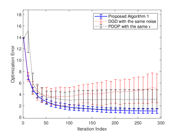
We consider a network of sensors interacting on the graph depicted in Fig. 1. In the evaluation, we set and . To evaluate the performance of the proposed Algorithm 1, we ignored the directions of edges in Fig. 1 in the selection of coupling weights and injected Laplace based DP-noise with parameter in every message shared in all iterations. We set the stepsize and diminishing sequence as and , respectively, which satisfy the conditions in Theorem 1 and Theorem 2. In the evaluation, we ran our algorithm for 100 times and calculated the average as well as the variance of the optimization error as a function of the iteration index. The result is given by the blue curve and error bars in Fig. 2. For comparison, we also ran the existing static-consensus based distributed gradient descent (DGD) approach in [6] under the same noise, and the differential-privacy approach for distributed optimization (PDOP) in [18] under the same privacy budget. Note that PDOP uses geometrically decreasing stepsizes (which are summable) to ensure a finite privacy budget, but the fast decreasing stepsize also leads to optimization errors. The evolution of the average optimization error and variance of the DGD and PDOP approaches are given by the red and black curves/error bars in Fig. 2, respectively. It is clear that the proposed algorithm has a comparable convergence speed but much better optimization accuracy.

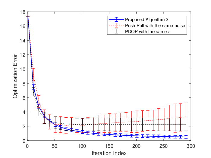
We also evaluated Algorithm 2 which is applicable to general directed graphs. More specifically, still using the topology in Fig. 1, we selected and matrices according to Assumption 4 and set the stepsize and diminishing sequences as , , and , respectively. We injected Laplace noises and (both have parameter ) on all shared and respectively to enable DP, and it can be verified that the parameters satisfy the conditions in Theorem 3 and Theorem 4. We ran our algorithm for 100 times and calculated the average as well as the variance of the optimization error as a function of the iteration index. The result is given by the blue curve and error bars in Fig. 3. For comparison, we also ran the conventional dynamic-consensus based Push-Pull method in [17] under the same noise and the PDOP based differential-privacy approach for distributed optimization. Because the PDOP based approach requires the stepsize to decay with a geometric rate, we set the stespize of Push-Pull to and used a geometrically decaying noise such that it has the same privacy budget as our approach. The evolution of the average optimization error and variance of Push Pull (with the same noise as our approach) and PDOP-privacy based Push Pull (with the same privacy budget as our approach) are depicted by the red and black curves/error bars in Fig. 3, respectively. It is clear that the proposed algorithm has a comparable convergence speed but gained significant improvement in optimization accuracy.
V-B Evaluation using image classification on MNIST
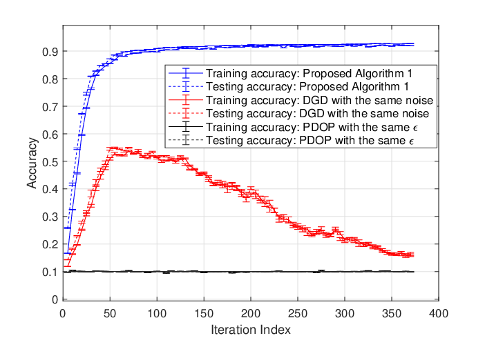
We also used decentralized training of a convolutional neural network (CNN) to evaluate the performance of our proposed algorithms. More specially, we consider five agents which collaboratively train a CNN using the MNIST dataset [45] under the topology in Fig. 1. The MNIST data set is a large benchmark database of handwritten digits widely used for training and testing in the field of machine learning [46]. Each agent has a local copy of the CNN. The CNN has 2 convolutional layers with 32 filters with each followed by a max pooling layer, and then two more convolutional layers with 64 filters each followed by another max pooling layer and a dense layer with 512 units. Each agent has access to a portion of the MNIST dataset, which was further divided into two subsets for training and validation, respectively. To evaluate the proposed Algorithm 1, We set the stepsize as and the weakening factor as . The Laplace noise parameter was set to to enable -DP. The evolution of the training and testing accuracies averaged over 50 runs are illustrated by the solid and dashed blue curves in Fig. 4. To compare the convergence performance of our algorithm with the conventional distributed gradient descent algorithm under DP-noise, we also implemented the distributed gradient descent (DGD) algorithm in [6] to train the same CNN using stepsize under the same Laplace noise. The results are illustrated by the solid and dotted red curves in Fig. 4. It can be seen that the proposed algorithm has much better robustness to DP-noise. Moreover, to compare with the existing DP approach for distributed optimization, we also implemented the DP approach PDOP in [39] on DGD under the same privacy budget . PDOP uses geometrically decaying stepsizes and noises to ensure a finite privacy budget. However, such fast-decaying stepizes turned out to be unable to train the complex CNN model (see training and testing accuracies in solid and dashed black curves in Fig. 4, respectively under and ). These comparisons corroborate the advantage of the proposed Algorithm 1.
To show the influence of DP-noise on the final optimization accuracy, we also scaled the noise by and respectively and obtained the training and testing accuracies. To compare the strength of enabled privacy protection, we ran the DLG attack model proposed in [21], which is the most powerful inference algorithm reported to date in terms of reconstructing exact raw data from shared gradient/model updates. The attacker was assumed to be able to observe all messages shared among the agents. The training/testing accuracies under different levels of DP-noise and DLG attacker’s inference errors are summarized in Table 1. It can be seen that there is a trade-off between privacy and accuracy under a fixed iteration number .
Algorithm 1 Algorithm 2 Noise Level11 1 Considering the noise in Fig. 4 and Fig. 5 as the base level for Algorithm 1 and Algorithm 2, respectively. Training Accuracy 0.951 0.925 0.859 0.924 0.921 0.910 Testing Accuracy 0.951 0.929 0.861 0.926 0.922 0.913 Final DLG Error 310.2 350.3 412.5 301.1 336.7 389.7
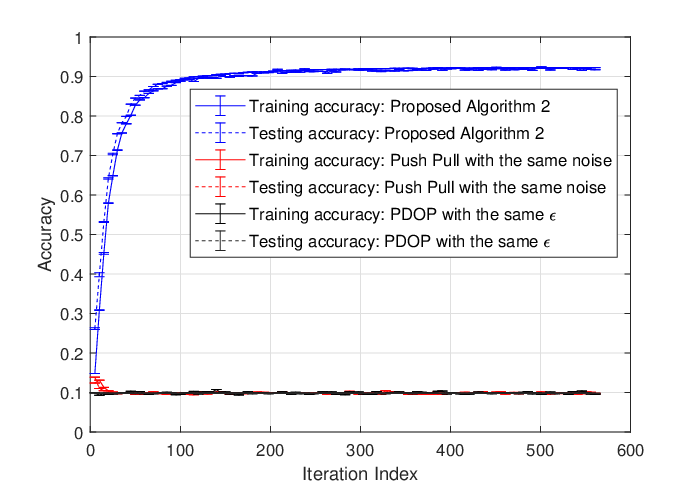
Using the same interaction topology, CNN network, and MNIST dataset, we also evaluated the performance of the proposed Algorithm 2 under DP-noise. The parameters of Algorithm 2 were set as , , , and . The Laplace noise parameter was set as . The evolution of the training and testing accuracies averaged over 50 runs are illustrated by the solid and dashed blue curves in Fig. 5. For comparison, we also implemented the dynamic-consensus based Push Pull algorithm in [17] to train the same CNN using stepsize under the same Laplace noise. The results are illustrated by the solid and dotted red curves in Fig. 5. It can be seen that the same amount of noise, which is tolerable to our proposed Algorithm 2, completely prevents the Push Pull algorithm from training the CNN model. Moreover, we also applied PDOP based DP approach in [39] to Push Pull, which uses geometrically decaying stepsizes and noises to ensure a finite privacy budget. However, under the same privacy budget, the fast-decaying stepize for Push Pull turned out to be unable to train the complex CNN model either (see Fig. 5 for training and testing accuracies in solid and dashed black curves, respectively, under and ). These comparisons corroborate the advantage of the proposed Algorithm 2.
To show the influence of DP-noise on the final optimization accuracy and the strength of enabled privacy, we also scaled the noise by and respectively and obtained the training/testing accuracies as well as DLG attacker’s inference errors. The results are given in Table 1, which shows a trade-off between privacy and accuracy under a fixed iteration number .
VI Conclusions, Discussions, and Future Work
Although DP is becoming the de facto standard for publicly sharing information, its direct incorporation into distributed optimization leads to significant reduction in optimization accuracy due to the need to iteratively and repeatedly inject independent noises. This paper proposes two DP-oriented gradient based distributed optimization algorithms that ensure both -DP and optimization accuracy. Specifically, the two algorithms can ensure almost sure convergence of all agents to the optimal solution even in the presence of persistent DP noise. Both algorithms are also proven able to ensure -DP with a finite cumulative privacy budget, even when the number of iterations goes to infinity. The simultaneous achievement of both provable convergence to the accurate solution and rigorous -DP with guaranteed finite cumulative privacy budget, to our knowledge, has not been reported before in distributed optimization. Numerical simulations and experimental results using a benchmark dateset confirm that both algorithms have a better accuracy compared with their respective existing counterparts, while maintaining a comparable convergence speed.
It is worth noting that our algorithms’ simultaneous achievement of both provable convergence to the optimal solution and -DP does not contradict the fundamental theory and limitations of DP in [27]. Firstly, our convergence guarantee (almost sure convergence) is obtained in the stochastic sense, which is different from deterministic convergence under no DP noise. More specifically, when the number of implementations tends to infinity, the concept of almost sure convergence still allows for a finite number of implementations that do not converge to the optimal solution. Secondly, according to the DP theory, conventional query mechanisms on a dataset can achieve -DP only by sacrificing query accuracies, but the distributed optimization algorithm does not correspond to a simple query mechanism on the optimal solution. Instead, what are queried in every iteration of distributed optimization are individual objective functions (gradients), and revealing the precise optimal solution is not equivalent to revealing accurate objective functions (the actual query target). In fact, in the language of machine learning, distributed optimization can be viewed as the empirical risk minimization problem, and the obtained optimal solution corresponds to the optimal model parameter in machine learning. On pages 216-218 of [27], the authors explicitly state that “the constraint of privacy is not necessarily at odds with the goals of machine learning, both of which aim to extract information from the distribution from which the data was drawn, rather than from individual data points,” and “we are often able to perform private machine learning nearly as accurately, with nearly the same number of examples, as we can perform non-private machine learning.” Actually, under Valiant’s model of machine learning (PAC), [27] notes that a model parameter (called function in [27]) is PAC learnable if and only if it is PAC learnable under DP (see page 221 of [27]). Thirdly, the achievement of -DP does incur utility cost. More specifically, in terms of Algorithm 1, in order to reduce to enhance privacy, we can use a faster-increasing according to Theorem 2, which requires to decrease faster according to Assumption 3. Given that the convergence speed is determined by according to Remark 3, we arrive at the conclusion that a faster decreasing corresponds to a stronger privacy level but a slower convergence speed. The same conclusion can be drawn for Algorithm 2. In future work, we will systematically quantify the cost of achieving DP in distributed optimization under the constraint of provable convergence to the optimal solution. Furthermore, we also plan to investigate if gradually reducing communication frequency can enable rigorous DP.
Acknowledgement
The authors would like to thanks Ben Liggett for the help in numerical experiments. They would also like to thank the associate editor and anonymous reviewers, whose comments helped improve the paper.
Appendix
VI-A Proof of Lemma 6
Let be an arbitrary but fixed optimal solution of problem (1). Then, we have for all . Hence, by letting , from relation (9) it follows a.s. that for all ,
| (22) |
Consider the vector and note . Thus, relation (22) satisfies all conditions of Lemma 5. So it follows that exists a.s., and that the sequences and are bounded a.s. From (22) we have the following relation a.s. for the second element of :
| (23) |
where . Since a.s. by our assumption, and the sequences and are bounded a.s., it follows that a.s. Thus, the preceding relation satisfies the conditions of Lemma 2 with , and due to our assumptions a.s. and . So one yields a.s.
| (24) |
It remains to show that a.s. For this, we consider relation (9) and focus on the first element of , for which we obtain a.s. for all :
| (25) | ||||
The preceding relation satisfies Lemma 3 with , , , , , and . By our assumptions, the sequences and are summable a.s., and . In view of (24), it follows that a.s. Hence, all the conditions of Lemma 3 are satisfied and, consequently, converges a.s. to some optimal solution.
VI-B Proof of Theorem 1
The basic idea is to apply Lemma 6 to the quantities and . We divide the proof into two parts to analyze and , respectively.
Part I: We first analyze . For the sake of notational simplicity, we represent as . Stacking and into augmented vectors and , respectively, we can write the dynamics of Algorithm 1 as
| (26) |
where denotes the Kronecker product, and with .
Using (27) and the preceding relation, we relate to an optimal solution
which further implies
Taking the conditional expectation, given , and using the assumption that the noise is with zero mean and variance conditionally on (see Assumption 3), from the preceding relation we obtain a.s. for all ,
| (28) | ||||
We next estimate the inner product term, for which we have
| (29) | ||||
Recalling that , by the Lipschitz continuous property of , we have
| (30) | ||||
By the convexity of , we have
| (31) | ||||
Combining (29), (30), and (31) leads to
| (32) | ||||
We next estimate the second last term in (28):
| (33) | ||||
Part II: Next we analyze . Using (26) and (27), we obtain
Noting , , and , we can rewrite the preceding equality as
| (37) |
with and .
Since holds and we always have , it follows that
By subtracting from the right hand side of (37), we obtain
which further leads to
where the inequality follows from and the definition . Taking the conditional expectation with respect to and using Assumption 3 yield
where . Using the fact and where is some non-zero eigenvalue of (see Assumption 2), we obtain
| (38) | ||||
for any , where we used valid for any scalars and .
We next focus on estimating the term involving the gradient in the preceding inequality. Noting and that has Lipschitz continuous gradients (with Lipschitz constant ), we have
Since , using the relationship in (34), we obtain
Finally, substituting the preceding relation back in (38) yields
By letting and consequently and , we arrive at
| (39) | ||||
By combining (36) and (39), and using Assumption 3, we have and satisfying the conditions of Lemma 6 with , , , and where .
VI-C Proof of Lemma 10
Since the results of Lemma 5 are asymptotic, they remain valid when the starting index is shifted from to , for an arbitrary . So the idea is to show that the conditions in Lemma 5 are satisfied for all (for some large enough ).
(a) Because for all , for to satisfy and , we only need to show that the following inequalities can be true
| (40) | ||||
The first inequality is equivalent to . Given that holds and as well as are positive according to the assumption, it can easily be seen that for any given , we can always find a satisfying the relationship when is larger than some .
The second inequality is equivalent to . Given that holds and as well as are positive according to the assumption, it can easily be seen that for any given , we can always find a satisfying the relationship when is larger than some .
The third inequality is equivalent to . Since the right hand side converges to zero according to our assumptions on , and , we can always find a constant satisfying this inequality for . Thus, we can always find a vector satisfying all inequalities in (40) for for some large enough , and hence the conditions in Lemma 5 are satisfied.
By Lemma 5, it follows that for the three entries of , i.e., , , and , we have that
| (41) |
exists a.s. and holds a.s. with . Since and , , and are summable, one has
| (42) |
Hence, it follows that
| (43) |
for some random scalars and due to the assumption .
Now, we focus on proving that both and converge a.s. to 0. The idea is to show that we can apply Lemma 8. By focusing on the second and third elements of , i.e., and , from (20) we have
where , , and , which can be rewritten as
where .
To apply Lemma 8, noting that and are not summable, we show that the equation has a solution in with and . From , one has
which can be simplified as , .
Given according to our assumption, it can be seen that is positive, and hence, such an and can always be found.
We next prove that the condition a.s. of Lemma 8 is also satisfied. Indeed, the condition can be met because: (1) , , , and are all summable according to the assumption of the lemma; and (2) (see (43)) and , , are all bounded a.s. due to the existence of the limit in (41). Thus, all the conditions of Lemma 8 are satisfied, so it follows that and a.s. Moreover, in view of the existence of the limit in (41) and the facts that and , it follows that exists a.s.
(b) Since holds a.s. (see (42)), from , it follows that we have a.s.
Now, if the function has bounded level sets, then the sequence is a.s. bounded since exists a.s. (as shown in part (a)). Thus, a.s. has accumulation points. Let be a sub-sequence such that a.s. Without loss of generality, we may assume that is a.s. convergent, for otherwise we would choose a sub-sequence of . Let . Then, by the continuity of the gradient , it follows , implying that is an optimal point. Since is continuous, we have . By part (a), exists a.s., so we must have a.s.
Finally, by part (a), we have a.s. for every . Thus, each has the same accumulation points as the sequence a.s., implying by the continuity of the function that a.s. for all .
VI-D Proof of Theorem 3
We divide the derivations into four steps: in Step I, Step II, and Step III, we establish relations for , , and for the iterates generated by Algorithm 2, respectively. In Step IV, we use them to show that (20) of Lemma 10 holds.
Step I: Relationship for .
Since is convex with Lipschitz gradients, we have
Letting and in the preceding relation and using (17), as well as , we obtain
We estimate the last term in the preceding inequality by using and . After subtracting on both sides of the resulting inequality, we obtain
Taking the conditional expectation with respect to yields
| (50) | ||||
where .
The inner product term in (50) satisfies
| (51) | ||||
where in the second equality we use valid for any vectors and .
Using the relationship
and the inequality , we can bound the first term on the right hand side of (51) as follows:
Using the inequality , we can bound the last term on the right hand side of (51) as follows:
Plugging the preceding two inequalities into (51) and combining the common terms lead to
| (52) | ||||
where in the last inequality we used and the assumption that each has Lipschitz continuous gradients with the constant .
Using the fact that in finite dimensional vector spaces, all norms are equivalent up to a proportionality constant, we always have a constant such that for all and hence according to the definition of matrix norm in (18). Similarly, we always have for some constant according to the definition of matrix norm in (19). Therefore, (53) can be rewritten as
| (54) |
Step II: Relationship for .
For the convenience of analysis, we write the iterates of (14) on per-coordinate expressions. Define for all
and ,
,
, , , . In
this per-coordinate view, (14) has the following form for all
and ,
| (55) | ||||
Noting that is the average of , i.e., , and abbreviating as , we have
where .
Taking norm on both sides leads to
where denotes the inner product induced22 2 It can be seen that the norm satisfies the Parallelogram Law and, hence, the inner product induced by the norm exists. by the norm .
Taking the expectation (conditioned on ) yields
| (56) | ||||
where in the last equality we used the relationship on the first term on the right hand side of (56) by setting to (resulting in ). Summing the preceding relations over , and noting , , , and , we obtain
| (57) | ||||
where is constant such that for all . (In finite dimensional vector spaces, all norms are equivalent up to a proportionality constant, represented by here.)
Step III: Relationship for .
From
(15), the th entries of
satisfy
Then, using (55), we obtain for all ,
where and . Note that we used the relationship .
Taking the norm on both sides yields
where in the inequality we used . Taking conditional expectation on both sides leads to
| (58) | ||||
where we used the relationship valid for any scalars and and set .
By summing these relations over , we find
| (59) | ||||
Using Assumption 6, we have
which, in combination with (59), yields
| (60) | ||||
where is constant such that for all . (In finite dimensional vector spaces, all norms are equivalent up to a proportionality constant, represented by here.)
Next, we proceed to analyze in (59). Using (14), we have for every index :
where we used in the second equality.
The preceding relationship leads to
where which is arbitrarily close to the spectral radius of the matrix .
By summing over , we obtain
| (61) | ||||
Step IV: We combine Steps I-III and prove the theorem.
From (15), we have
which further implies
and
Given that is summable according to the theorem statement, and is not summable but square summable, we have that satisfies the condition in Lemma 2. Therefore, the sequence is summable a.s. according to Lemma 2, and hence, is summable a.s. under the theorem condition .
Using Assumption 5, and the conditions that , , , and are summable in the theorem statement, it follows that all entries of the matrix are a.s. summable. By defining as the maximum element of , we have . Therefore, , , and for the iterates generated by Algorithm 2 satisfy the conditions of Lemma 10 and, hence, the results of Lemma 10 hold.
References
- [1] T. Yang, X. Yi, J. Wu, Y. Yuan, D. Wu, Z. Meng, Y. Hong, H. Wang, Z. Lin, and K. H. Johansson, “A survey of distributed optimization,” Annual Reviews in Control, vol. 47, pp. 278–305, 2019.
- [2] J. A. Bazerque and G. B. Giannakis, “Distributed spectrum sensing for cognitive radio networks by exploiting sparsity,” IEEE Transactions on Signal Processing, vol. 58, no. 3, pp. 1847–1862, 2009.
- [3] C. Zhang and Y. Wang, “Distributed event localization via alternating direction method of multipliers,” IEEE Transactions on Mobile Computing, vol. 17, no. 2, pp. 348–361, 2017.
- [4] K. I. Tsianos, S. Lawlor, and M. G. Rabbat, “Consensus-based distributed optimization: Practical issues and applications in large-scale machine learning,” in Proceedings of the 50th annual Allerton Conference on Communication, Control, and Computing, 2012, pp. 1543–1550.
- [5] J. N. Tsitsiklis, “Problems in decentralized decision making and computation.” MIT, Tech. Rep., 1984.
- [6] A. Nedic and A. Ozdaglar, “Distributed subgradient methods for multi-agent optimization,” IEEE Transactions on Automatic Control, vol. 54, no. 1, pp. 48–61, 2009.
- [7] K. Srivastava and A. Nedic, “Distributed asynchronous constrained stochastic optimization,” IEEE Journal of Selected Topics in Signal Processing, vol. 5, no. 4, pp. 772–790, 2011.
- [8] W. Shi, Q. Ling, G. Wu, and W. Yin, “EXTRA: An exact first-order algorithm for decentralized consensus optimization,” SIAM Journal on Optimization, vol. 25, no. 2, pp. 944–966, 2015.
- [9] J. Xu, S. Zhu, Y. C. Soh, and L. Xie, “Convergence of asynchronous distributed gradient methods over stochastic networks,” IEEE Transactions on Automatic Control, vol. 63, no. 2, pp. 434–448, 2017.
- [10] G. Qu and N. Li, “Harnessing smoothness to accelerate distributed optimization,” IEEE Transactions on Control of Network Systems, vol. 5, no. 3, pp. 1245–1260, 2017.
- [11] R. Xin and U. A. Khan, “A linear algorithm for optimization over directed graphs with geometric convergence,” IEEE Control Systems Letters, vol. 2, no. 3, pp. 315–320, 2018.
- [12] W. Shi, Q. Ling, K. Yuan, G. Wu, and W. Yin, “On the linear convergence of the ADMM in decentralized consensus optimization,” IEEE Transactions on Signal Processing, vol. 62, no. 7, pp. 1750–1761, 2014.
- [13] C. Zhang, M. Ahmad, and Y. Wang, “ADMM based privacy-preserving decentralized optimization,” IEEE Transactions on Information Forensics and Security, vol. 14, no. 3, pp. 565–580, 2019.
- [14] E. Wei, A. Ozdaglar, and A. Jadbabaie, “A distributed Newton method for network utility maximization–I: Algorithm,” IEEE Transactions on Automatic Control, vol. 58, no. 9, pp. 2162–2175, 2013.
- [15] K. Yuan, Q. Ling, and W. Yin, “On the convergence of decentralized gradient descent,” SIAM Journal on Optimization, vol. 26, no. 3, pp. 1835–1854, 2016.
- [16] P. Di Lorenzo and G. Scutari, “NEXT: In-network nonconvex optimization,” IEEE Transactions on Signal and Information Processing over Networks, vol. 2, no. 2, pp. 120–136, 2016.
- [17] S. Pu, W. Shi, J. Xu, and A. Nedić, “Push-pull gradient methods for distributed optimization in networks,” IEEE Transactions on Automatic Control, vol. 66, no. 1, pp. 1–16, 2021.
- [18] Z. Huang, S. Mitra, and N. Vaidya, “Differentially private distributed optimization,” in Proceedings of the 2015 International Conference on Distributed Computing and Networking, 2015, pp. 1–10.
- [19] D. A. Burbano-L, J. George, R. A. Freeman, and K. M. Lynch, “Inferring private information in wireless sensor networks,” in IEEE International Conference on Acoustics, Speech and Signal Processing, 2019, pp. 4310–4314.
- [20] F. Yan, S. Sundaram, S. Vishwanathan, and Y. Qi, “Distributed autonomous online learning: Regrets and intrinsic privacy-preserving properties,” IEEE Transactions on Knowledge and Data Engineering, vol. 25, no. 11, pp. 2483–2493, 2012.
- [21] L. Zhu, Z. Liu, and S. Han, “Deep leakage from gradients,” in Advances in Neural Information Processing Systems, 2019, pp. 14 774–14 784.
- [22] C. Zhang and Y. Wang, “Enabling privacy-preservation in decentralized optimization,” IEEE Transactions on Control of Network Systems, vol. 6, no. 2, pp. 679–689, 2018.
- [23] N. M. Freris and P. Patrinos, “Distributed computing over encrypted data,” in 2016 54th Annual Allerton Conference on Communication, Control, and Computing (Allerton). IEEE, 2016, pp. 1116–1122.
- [24] Y. Lu and M. Zhu, “Privacy preserving distributed optimization using homomorphic encryption,” Automatica, vol. 96, pp. 314–325, 2018.
- [25] Y. Lou, L. Yu, S. Wang, and P. Yi, “Privacy preservation in distributed subgradient optimization algorithms,” IEEE Transactions on Cybernetics, vol. 48, no. 7, pp. 2154–2165, 2017.
- [26] S. Gade and N. H. Vaidya, “Private optimization on networks,” in American Control Conference. IEEE, 2018, pp. 1402–1409.
- [27] C. Dwork, A. Roth et al., “The algorithmic foundations of differential privacy.” Foundations and Trends in Theoretical Computer Science, vol. 9, no. 3-4, pp. 211–407, 2014.
- [28] S. Han, U. Topcu, and G. J. Pappas, “Differentially private distributed constrained optimization,” IEEE Transactions on Automatic Control, vol. 62, no. 1, pp. 50–64, 2016.
- [29] M. T. Hale and M. Egerstedt, “Cloud-enabled differentially private multiagent optimization with constraints,” IEEE Transactions on Control of Network Systems, vol. 5, no. 4, pp. 1693–1706, 2017.
- [30] Y. Wang, Z. Huang, S. Mitra, and G. E. Dullerud, “Differential privacy in linear distributed control systems: Entropy minimizing mechanisms and performance tradeoffs,” IEEE Transactions on Control of Network Systems, vol. 4, no. 1, pp. 118–130, 2017.
- [31] X. Zhang, M. M. Khalili, and M. Liu, “Recycled admm: Improving the privacy and accuracy of distributed algorithms,” IEEE Transactions on Information Forensics and Security, vol. 15, pp. 1723–1734, 2019.
- [32] J. He, L. Cai, and X. Guan, “Differential private noise adding mechanism and its application on consensus algorithm,” IEEE Transactions on Signal Processing, vol. 68, pp. 4069–4082, 2020.
- [33] J. Cortés, G. E. Dullerud, S. Han, J. Le Ny, S. Mitra, and G. J. Pappas, “Differential privacy in control and network systems,” in IEEE 55th Conference on Decision and Control (CDC), 2016, pp. 4252–4272.
- [34] Y. Xiong, J. Xu, K. You, J. Liu, and L. Wu, “Privacy preserving distributed online optimization over unbalanced digraphs via subgradient rescaling,” IEEE Transactions on Control of Network Systems, 2020.
- [35] T. Ding, S. Zhu, J. He, C. Chen, and X.-P. Guan, “Differentially private distributed optimization via state and direction perturbation in multi-agent systems,” IEEE Transactions on Automatic Control, 2021.
- [36] E. Nozari, P. Tallapragada, and J. Cortés, “Differentially private distributed convex optimization via functional perturbation,” IEEE Transactions on Control of Network Systems, vol. 5, no. 1, pp. 395–408, 2016.
- [37] B. Polyak, “Introduction to optimization,” Optimization software Inc., Publications Division, New York, vol. 1, 1987.
- [38] K. L. Chung, “On a stochastic approximation method,” The Annals of Mathematical Statistics, pp. 463–483, 1954.
- [39] Z. Huang, S. Mitra, and N. Vaidya, “Differentially private distributed optimization,” in Proceedings of the 2015 International Conference on Distributed Computing and Networking, New York, NY, USA, 2015.
- [40] S. Kar and J. M. Moura, “Distributed consensus algorithms in sensor networks with imperfect communication: Link failures and channel noise,” IEEE Transactions on Signal Processing, vol. 57, no. 1, pp. 355–369, 2008.
- [41] R. A. Horn and C. R. Johnson, Matrix analysis. Cambridge university press, 2012.
- [42] P. Kairouz, S. Oh, and P. Viswanath, “The composition theorem for differential privacy,” in International Conference on Machine Learning. PMLR, 2015, pp. 1376–1385.
- [43] M. Bun and T. Steinke, “Concentrated differential privacy: Simplifications, extensions, and lower bounds,” in Theory of Cryptography Conference. Springer, 2016, pp. 635–658.
- [44] I. Mironov, “Rényi differential privacy,” in The 30th Computer Security Foundations Symposium. IEEE, 2017, pp. 263–275.
- [45] Y. LeCun, C. Cortes, and C. Burges, “The MNIST database of handwritten digits,” http://yann.lecun.com/exdb/mnist/, 1994.
- [46] L. Deng, “The MNIST database of handwritten digit images for machine learning research,” IEEE Signal Processing Magazine, vol. 29, no. 6, pp. 141–142, 2012.