Giga-scale Kernel Matrix-Vector Multiplication on GPU
Abstract
Kernel matrix-vector multiplication (KMVM) is a foundational operation in machine learning and scientific computing. However, as KMVM tends to scale quadratically in both memory and time, applications are often limited by these computational constraints. In this paper, we propose a novel approximation procedure coined Faster-Fast and Free Memory Method () to address these scaling issues of KMVM for tall () and skinny () data. Extensive experiments demonstrate that has empirical linear time and memory complexity with a relative error of order and can compute a full KMVM for a billion points in under a minute on a high-end GPU, leading to a significant speed-up in comparison to existing CPU methods. We demonstrate the utility of our procedure by applying it as a drop-in for the state-of-the-art GPU-based linear solver FALKON, improving speed 1.5-5.5 times at the cost of drop in accuracy. We further demonstrate competitive results on Gaussian Process regression coupled with significant speedups on a variety of real-world datasets.
1 Introduction
Kernel matrix-vector multiplication (KMVM) is one of the most important operations needed in scientific computing with core applications in diffeomorphic registration, geometric learning Charlier et al. 2020, Tward et al. 2020, numerical analysis Schwab and Wendland 1992, fluid dynamics Belley et al. 2009, and machine learning Scholkopf and Smola 2001. For a dataset of size , KMVM using direct computation has complexity and memory footprint , both unfeasible for modern large scale applications where is becoming increasingly common. Pioneering contributions presented in the Fast Multipole Method (FMM) Carrier et al. 1988 amend the complexity of these problems to , where is the chosen error tolerance, with varying reductions in memory footprint for data restricted to dimension . Subsequent developments in Börm et al. 2019; Greengard et al. 2020 mainly focused on extending approximations for a broader set of kernels for a fixed dimensionality , tailored for problems in physics with narrow data such as electrostatics, stellar dynamics, Stokes flow, and acoustic problems, amongst others.
In this paper, we introduce Faster-Fast and Free Memory Method (F3M), a novel algorithm built upon the FFM Aussal and Bakry 2019 framework to perform KMVM on a GPU for tall and skinny () data of order in under a minute with user-specified error tolerance, providing between times speed-up over existing methods. It should be noted that the constraints on and are not inherent formal constraints, but a reflection of practical limits with typical current computational resources.
Notations. We use capital and lower case bold letters to represent matrices and vectors, respectively. In this paper, we will work with matrices , and vector . For a kernel , the goal for KMVM is to compute , where , and denote the row of respectively.
2 Motivation and Related Work
Kernel methods are often limited by their memory footprint and computational complexity for KMVM. These constraints make scaling beyond challenging. Many recent developments have been made to improve both of these constraints, ranging from hardware acceleration using GPUs in KeOps Charlier et al. 2020, to various approximation techniques proposed in Yang et al. 2003; Wang et al. 2019b; Wilson and Nickisch 2015a; Aussal and Bakry 2019; Cai et al. 2017. In this work, we focus our attention on kernel independent KMVM methods.
KeOps. Charlier et al. (Charlier et al. 2020) proposes a map-reduce scheme to compute kernels using exactly memory and complexity on GPU. This is achieved by computing the full KMVM product on-the-fly by summing directly, without ever storing the kernel matrix explicitly. Extensive experiments show that this method is practical when , as the GPU hardware acceleration allows the KMVM product to be computed in less than a second on a conventional GPU. Moreover, the method places no constraint on the number of features it can be applied to, making it favourable for KMVM on medium size datasets. In application contexts, KeOps is currently adopted into conjugate gradient solver FALKON Meanti et al. 2020; Rudi et al. 2018 as part of the default pipeline.
| Method | FMM | KeOps | FFM | ||||
| Kernel Independent | ✓ | ✓ | ✓ | ✓ | |||
| Linear Time | ✓ | ✓ | ✓ | ✓ | |||
| Linear Memory | ✓ | ✓ | ✓ | ✓ | |||
| Restriction in | |||||||
| GPU | ✓ | ✓ | ✓ | ✓ | |||
|
✓ | ✓ | |||||
| under 1 minute! 22footnotemark: 2 | ✓ |
The Fast and Free Memory Method (FFM). While KeOps can theoretically scale to a billion points, it becomes practically infeasible as the complexity would imply a computational time of seconds, or roughly days. To overcome this billion points barrier, Aussal et al. Aussal and Bakry 2019 deploys a geometric space partitioning scheme, and proposed the Fast and Free Memory Method (FFM), a KMVM approach that extends the FMM Carrier et al. 1988 family of algorithms. In contrast to traditional FMM methods, which require specific series expansion of the kernel, FFM deploys Lagrange interpolations to approximate them instead. This allows FFM to be applied to almost any conventional kernel and further enables the user to trade off accuracy with computational efficiencies by controlling the order of the approximating polynomial Howell 1991. Compared to KeOps, FFM demonstrates both linear memory and time complexity in experiments and scales to compute a billion-points KMVM on a smaller CPU cluster under hours, outscaling the GPU implementation of FMM Kohnke et al. 2020. While hours is a significant improvement compared to days from KeOPS, it still renders many machine learning techniques infeasible. Further, as recursive partitioning of the data space scales poorly with Barnes and Hut 1986, both FMM and FFM can only be applied to data, a price to pay for the speed-up of KMVM operations when . Furthermore, we show in our experiments that a direct FFM port to GPU gives unstable results for for non-trivial data simulations (bottom row in Appendix 10).
Our contribution. To surpass the billion point barrier while maintaining high-speed and stable computation, we propose and our main algorithm , the first pair of KMVM algorithms that can reliably scale to on skinny data using a single GPU. We build on top of FFM by introducing non-trivial GPU parallelisation and low-level optimisations. We further stabilize and improve the original geometric partitioning scheme in FFM to significantly reduce memory constraints, leading to a relaxation of dimensionality constraints from to . At last, we introduce an adaptive far-field and smooth field approximation scheme for kernel interpolation, resulting in our main algorithm , which runs times quicker and more stable than a direct port of FFM on GPU. See Fig. 1 and Table 1 for an overview and comparisons of the methods. We summarise our contribution as follows:
1. We propose Faster-Fast and Free Memory Method , a KMVM algorithm building on top of FFM by applying multiple low-level enhancements, GPU parallelisation, and algorithmic computational and memory enhancements, allowing for KMVM operations on data in under a minute. Codebase is released here for F3M.
2. We characterize theoretical time and memory complexity of .
3. We run extensive KMVM experiments of on a variety of tall and skinny data with , demonstrating empirical linear time and memory scaling, and achieving speedups between 2–8500 times when compared to FFM (GPU and CPU) and KeOps.
4. We run a practical application of as a drop-in replacement for KeOps in conjugate gradient solver FALKON Meanti et al. 2020; Rudi et al. 2018 for kernel ridge regression and classification (KRR) on giga-scale data, obtaining a solution 3.4 times faster with <1% drop in accuracy. We further demonstrate competitive results on Gaussian process regression against KISS-GP Wilson and Nickisch 2015b, SVGP Hensman et al. 2013 and SVGR Titsias 2009 with significant speed-ups.
3 Background
The FFM method considers KMVM for a kernel evaluated on two data matrices and are weights associated with .


The KMVM is expressed as . For example, could be the weights in a KRR or the strength of electronic charges. As and are taken to be very large, a full computation is unfeasible. In this section, we illustrate and detail the main steps of FFM, before presenting our improvements in Section 4.
For illustration purposes, we first consider a simple 2D KMVM. Our goal is to calculate for in Figure 2. The intuition behind FFM is to reduce the complexity of calculating the full KMVM by partitioning and such that certain calculations can be approximated in a fast manner, based on the pairwise distances between partitions.
Enclosing and partitioning the data. The first step is to partition the data. To begin, we find a large enough box that can just enclose or . The edge length of this box is calculated as
where denotes the largest value and the smallest value along the -dimension in and similarly for . Figure 2 illustrates this enclosing procedure.
Defining near and far-field In FMM, an octree Meagher 1980 is applied to recursively partition data into
smaller boxes , with denoting box indices. Here each box corresponds to a subset of rows in the data matrix. Let us also denote as the partition of ’s grouped with the same indices as . To calculate the KMVM between two boxes with the grouped vector , for each , we compute
| (1) |
with . Now the target can be computed as , where , denote the total number of boxes and a permutation such that appear in the same order as appears in . Figure 3 shows how boxes are recursively partitioned.

Far and near-field interactions FFM relies on a divide-and-conquer strategy to effectively compute a KMVM product; data is partitioned into boxes and then separated into far-field and near-field interactions, where near-field interactions are computed exactly and far-field interactions are approximated using Lagrange interpolation for speed, explained in the paragraph below. The partitioning procedure in FFM is recursive, where the recursion depth tree_depth controls the size of the edge of the box. An interaction is defined to be in the far-field if the distance between the two center points of the boxes exceeds , i.e. . While for each box will decrease with the number of divisions, this rule ensures a fixed minimal distance for a given depth for far-field interactions. Figure 3 illustrates how far(green) and near(orange)-field interactions arise between and when tree_depth increases.
Lagrange interpolation We review Lagrange interpolation used for far-field approximations in FFM. Given a function and unique points , there exists a unique polynomial of degree that interpolates at . The Lagrange polynomial is given by where We are free to chose the degree as well as the points to interpolate through. The choice of is especially important in minimizing large oscillations around the edges of the interpolation interval (Runge’s phenomenon Epperson 1987). For this reason, Chebyshev nodes of the second kind are used Berrut and Trefethen 2004 .
Interpolating By noticing that is a bivariate function, we can apply Lagrange interpolation twice, thus interpolating as Here denotes the number of the interpolation nodes and denotes the grid of interpolation nodes for and . Note that since , we take These operations can be vectorized and computed sequentially on-the-fly with linear memory footprint , which is done by first computing , then and lastly v. Here denotes a matrix with entries , where indexes the rows and the columns, with following the same definition for ’s instead. A far-field KMVM between two boxes is then approximated by using double Lagrange interpolation according to Figure 4.

4 Faster-FFM ( and )
To fully leverage the port of FFM to GPU, we enhance FFM with novel approximation procedures for improved complexity and memory optimizations to scale to . We coin this improved version Faster-FFM (). The capabilities of against previous methods are summarized in Table 1.
4.1 CPU to GPU optimizations
In FFM, every computation is serial and on CPU. When moving to GPU, we have parallelized all major computations. These parallelizations are non-trivial and require low-level algorithmic optimizations, with challenges such as:
Box-to-threadblock alignment – A major challenge in the implementation of both the parallel far-field and near-field computations was correctly aligning thread blocks to boxes. This aligning requirement imposed non-trivial boundary conditions on data indexing when using shared memory. To minimize memory usage of box and block indicators for our implementation, we represented the box belonging of each point as index intervals (i.e. box 1 consists of points with and box 2 with , etc.) and modulo arithmetic to infer the block belonging. This clearly requires that the points are sorted or grouped according to their box belonging. However, as we detail in the next paragraph, arranging the points could not be done straightforwardly with native sorting methods. We further illustrate how parallelization is done for calculating near-field interactions in Appendix I.
No native sorting methods – We found that LibTorch (Paszke et al. 2019) sorting methods often led to out-of-memory (OOM) due to allocation of large long-type vectors on GPU. When , this implies
allocating 8GB of memory, 25% of the 32GB card used, making it a necessity to avoid native sorting methods.
In-place grouping data on boxes – Due to infeasible LibTorch sorting methods, we additionally had to design an algorithm that finds a permutation that would group into its corresponding boxes in linear time and memory. We used a count and increment-based strategy that would:
1. Count the number of points in each box during the assignment operation () and store the count in a vector . Then run a cumulative sum over , starting from 0.
2. Initialize a long permutation vector . Using the counting vector , we would re-run the assignment operation and arrange a point with index as following , where is a running count of points in each box. We specifically have to use the function atomicAdd to increment the count for each box in parallelized GPU environments to avoid thread locks.
We refer to the box_division_cum_hash and box_division_assign_hash function in n_tree.cu for exact details.
Ensuring interactions are sorted – To avoid any unnecessary sorting, we ensure that the matrix containing interactions is always sorted by recursively dividing old interactions. We illustrate the procedure in Figure 5. We refer to the get_new_interactions function in n_tree.cu for the exact implementation.
However, we found that these optimizations and porting alone were not enough to scale to on 3D datasets, as Figure 6 demonstrates. FFM doesn’t remove empty boxes or handle boxes with few points in them and keeps exponentially creating new empty boxes and interactions, thus leading to out-of-memory (OOM) errors on non-uniform data (see Appendix 10).
4.2 Scaling to on GPU ()
In this section, we detail the memory enhancements that allow to consistently scale to .

Removing empty boxes with hash list indexing To ensure linear memory on GPU, we only keep a reindexing vector of size (resp. ) in memory during the computation of the algorithm in addition to a list of interactions and box centers. This reindexing vector rearranges the data points so they appear in the order of the box they belong to. We optimize both the computation and the memory footprint of these objects by avoiding recursive formulas and hash lists.
Naively, points can be assigned to boxes by direct comparison to all existing box centers. As the number of centers grows exponentially with depth tree_depth, this method quickly becomes pathological. To amend this, we propose a linear complexity formula to retrieve the box index a point belongs to where denotes the minimum value of in dimension and is the value of in dimension . To prevent the number of boxes from growing exponentially, we remove empty boxes with each division. To assign points to the corresponding boxes, we use a hash list to store and the order . We can then group points to their respective ordering using the hash list in time in contrast to by direct computation.
Handling boxes with few points with small field In cases when the number of points in each box can vary greatly, we separately consider the interactions where the number of points in boxes is small. Hence, we say that there is a small field interaction between boxes if both have a small number of points, i.e. if
, for some threshold number . To minimize the computations needed, can be set to . This intuitively allows to directly compute interactions that are too small to benefit from interpolation savings (i.e. ), thus limiting memory usage by stopping partitions from dividing further than necessary. In higher dimensions where the division rate is faster, can be set to a higher value to limit memory usage at the expense of more direct computations which are slower.
Sparse grids As the number of Lagrange polynomials increases exponentially with dimension, we implement sparse grids Smolyak 1963 to allow for a finer selection of interpolation nodes. With sparse grids, the number of nodes needed grows slower Kang and Wilcox 2015, thus saving memory. We give an example of a sparse grid versus a full grid in 2D in Figure 7.
4.3 Speeding up
Smoothness criteria FFM speeds up its computations with minimal loss in accuracy by selectively interpolating interactions that are far apart. To improve speed, we introduce the smoothness criterion to widen the selection of interactions that can be interpolated with minimal loss in accuracy. For a Gaussian Kernel , with lengthscale , the smoothness criteria is defined as
between an adjacent interaction of boxes , . The quantity computed can be understood as “Effective Variance” (EV), as it considers total variation in the exponent of the Gaussian kernel. We justify the smoothness criteria with the following proposition.
Proposition 1.
Consider such that for all . When interpolating using bivariate Lagrange interpolation with degree , for any there exist nodes for such that the pointwise interpolation error is bounded by .


See Appendix D for proof. Hence for small , we see that the error becomes small for well specified . To avoid calculating the sample variance during computations which costs , we exploit that data is partitioned into hypercubes with a known edge and take the upper bound of the variance in each cube as along a dimension. A proof for this bound is provided in Appendix B. Adjacent interactions are then classified as smooth when which only costs to compute.
Adaptive far-field approximation To further improve speed we introduce an adaptive rule to select the number of interpolation nodes used when calculating far-field interactions. Error bounds for multidimensional Lagrange interpolation have been proposed in Leaf and Kaper 1974, however, these bounds cannot be directly used to create an adaptive interpolation rule. We thus simulate KMVM errors for where are uniformly distributed and is normally distributed. We fix a distance between and and vary the squared of this distance between boxes against nodes in Figure 8. We use a Gaussian Kernel with .
Based on Figure 8, we use the following rule for selecting the number of interpolation nodes for far-field interactions
where is the number of nodes chosen to interpolate with in the general case.
Barycentric lagrange interpolation We slightly improve the complexity further by implementing barycentric Lagrange interpolation Berrut and Trefethen 2004 evaluated at the Chebyshev nodes of the second kind. As this is a well-known technique, we refer to the appendix for more details. It should be noted that the above methods can straightforwardly be extended to any translation-invariant kernel by recalculating the Taylor expansion for smoothness criteria and rerunning the simulation for adaptive far-field approximation.
4.4 Complexity
The time complexity of FFM is Aussal and Bakry 2019 and we use a similar derivation strategy for to obtain a complexity that is dependent on the effective variance limit (chosen parameter) and the box width (data). We first present two propositions needed to derive the complexity of .
Proposition 2.
A far-field interaction between two boxes containing and points respectively has time complexity , where .
Proposition 3.
Given data points in dimension , the maximum number of divisions is given by
| (2) |
With the above results, the complexity of FFM is taken as the maximum number of divisions multiplied by the complexity of far-field interactions at each division which yields . We remark that near-field interactions between boxes containing only 1 data point have linear time complexity, hence the results hold.
Theorem 1.
Given a KMVM with edge (dependent on data ), lengthscale , effective variance limit , data points and data dimension , has time complexity , which can be taken as where .
Memory footprint As our implementation uses the same partitioning strategy as FFM, the theoretical memory complexity remains for (see Aussal and Bakry 2019 for proof). However, this does not accurately reflect the memory footprint of the actual implementations, whose memory mostly depends on the number of interactions stored. We summarize these memory footprints for FFM and in Theorem 2 below.
Theorem 2.
The number of interactions against tree depth of FFM and grows as and
respectively. Here and and denotes the number of far-field, smooth field, small field interactions and the number of empty boxes respectively at depth .
We see that the additional approximations presented in also impacts memory footprint, as the additional terms removes a substantial amount of interactions at each , significantly slowing down the growth of interactions, reducing memory growth. The efficacy of is widely dependent on data. As an example, data with points very close to each other would significantly benefit more, as the closeness of points would imply more smooth interactions. If points are sparsely spread out, would provide the most benefit as they remove empty boxes and stops boxes with few points to divide unnecessarily. All proofs can be found in Appendix E.
5 Experiments
We demonstrate the utility of over a variety of experiments using the Gaussian kernel .22 2 is kernel agnostic, however we choose the Gaussian kernel for simplicity. We generate data such that the EV (see section 4.3) varies between for data of sizes . The parameters used for are and with a cap at . The error for the approximated KMVM product is calculated as , where the true KMVM product is obtained by calculating the full KMVM on a subset consisting of the first 5000 points in against the entire dataset in double precision, i.e. , where we fix . All experiments were run on NVIDIA V100-32GB cards, where the data is fitted entirely on the GPU. These cards were chosen since the extra graphic memory is necessary to fit the data on one card when . It should be noted that can only be run up to , as and itself cannot fit in memory for higher dimensions with the GPUs we had available. For details on how scales across multiple GPUs, see Appendix G.
| FFM (12 CPU cores) | (GPU, Ours) | ||||||
| n | Time (s) | Error | Memory | Time (s) | Error | Memory | Speedup |
| 100 MB | 28 MB | ||||||
| 1GB | 280 MB | ||||||
| 10 GB | 2.8 GB | ||||||
| 100 GB | 28 GB | ||||||
| Time(s) | Relative Error | |||||||||||||
| 1 | 2 | 3 | 4 | 5 | 6 | 7 | 1 | 2 | 3 | 4 | 5 | 6 | 7 | |
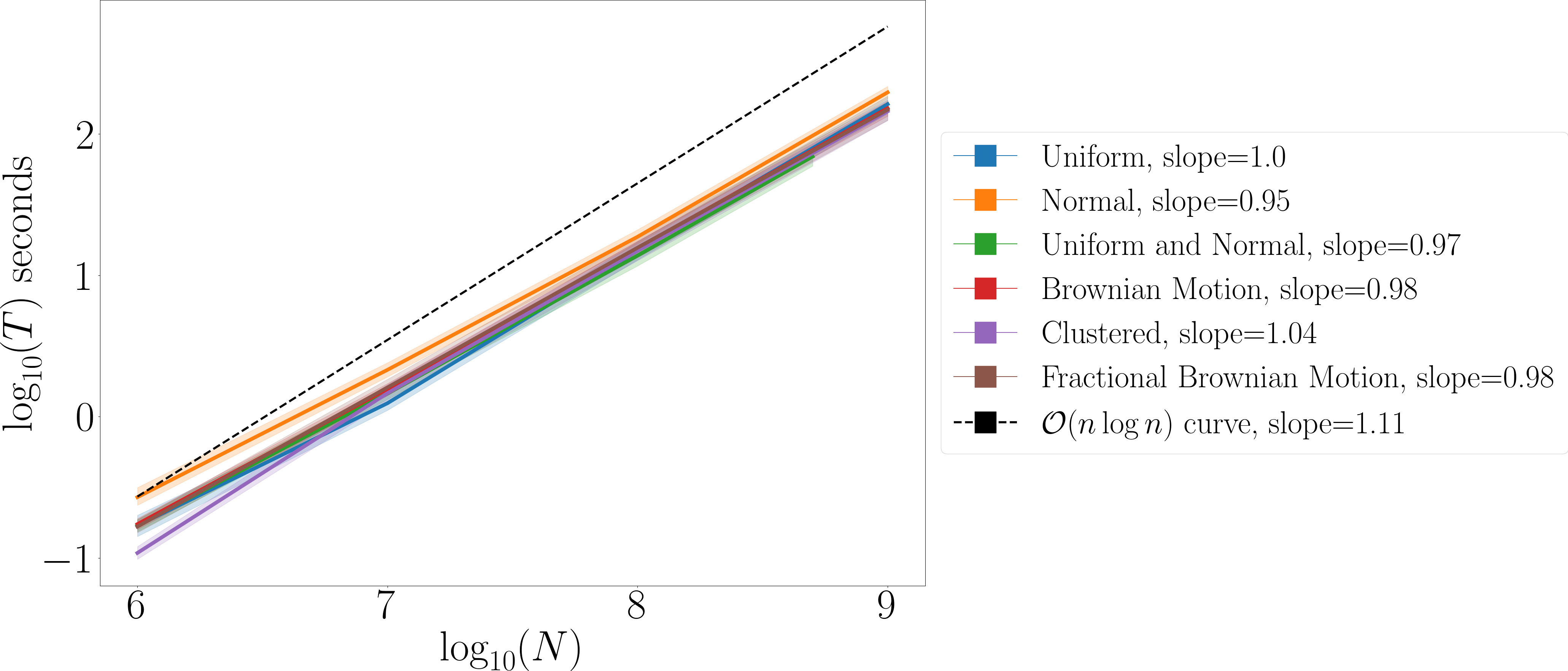
KMVM experimentsWeconsiderawidevariationofgenerateddatasetstosimulatedifferentreal-worldscenariostotestF^3Mon.Forthek(X,X)-caseweconsideruniformlyandnormallydistributeddata(D=1,2,3,4,5,6,7)togetherwithdatasimulatedfromBrownianmotion,fractionalBrownianmotion,andClustereddata(D=1,2,3).Forthek(X,Y)-caseweconsideruniformlydistributedxandnormaldistributedy(D=1,2,3,4,5,6,7).SeeAppendix10forvisualizationsofdata.Wehavetoconsidersmallernforthek(X,Y)-casewhenD≥3,astwicetheamountofdataneedstobestored.ForD=3/(4,5)/(6,7)weinsteadconsideratmostn=5⋅10^8/2.5⋅10^8/10^8.ItshouldbenotedthatD=7isahardlimitforgeometricpartitioning-basedmethods,sinceforD=8,wewouldhave2^8⋅2 ⋅2^8⋅2≈4.3 ⋅10^9interactionsafteronly2divisions.Thisnumberofinteractionscannotevenberepresentedbya32-bitinteger.WesummarizetherunsinSection 5andplottheerrorandtimecomplexityinFigure 9foreachdatasetwhenD=3.WefindthatF^3Mmaintainssub-linearempiricalcomplexityuptoD=6,wherewehavetosetsmallfieldlimitρtoalargernumbertonotrunoutofmemory.Further,theerrorincreasesinthehigherdimensionssinceweusefewernodesperdimensionwheninterpolating,owingtothesparsegridtechnique.WenotethatD=7hasfasterruntimesthanD=6whichisexplainedbythatforsomevaluesofEV,D=7doesn ′ trunwithacceptableerrorswhichskewtheruntimetodatasetswherealargerportionofthedatacanbeinterpolated.

WefurtherreplicatethedatausedinthefirstexperimentinAussal and Bakry 2019andcompareF^3MagainstFFM(CPU)inTable 2.
Kernel Ridge Regression experimentWeapplyF^3MtoFALKONMeanti et al. 2020,wherewereplacetheirKMVMoperationwithF^3MandcompareperformanceandspeedinsolvingKernelRidgeRegression(KRR).TheKMVMoperationcurrentlyusedforsmallerdimensionsisKeOpsCharlier et al. 2020.GivensomedataX∈R^N×dwewanttofindthesolutionα = ( k(X,X)+λI )^-1bwhereλistheridgeparameterthatstabilizestheinverse.FALKONisaNyströmapproximationbasedsolverthatrequiresasubsampleX’∈R^M×dofXtoapproximatetheinversecomputation.Wefocustheexperimentsontallandskinnydataandtaken=10^9, d≤3withM=10^5forallexperiments.Weconsideruniformlyandnormallysampleddata,theOpenStreetMap(OSM)datasetosmandaclassificationtaskontheNYCTaxidataset tax,wherewepredictwhetherthecustomerwilltipbasedontripdistance,triptimeandfarecost.Toconstructbonsyntheticproblems,wefirsttakeasubsetD∈R^1000×dofXandsampleα∼N(0,I_1000×1000).Wethencalculateb=k(X,D)⋅α+ ε,whereε∼N(0,0.1).WerunKRRforEV=0.1,1,10onsyntheticdata,andreporttheaverageR^2(AUCforNYCTaxi)andtrainingtimeinTable 4.FortherealworlddatasetsOSMandNYCTaxi,wefixthelengthscaleusingthemedianheuristicproposedinGarreau et al. 2017averagedourresultsoverthe3runs.
| FALKON with default KMVM | FALKON with | ||||||||
| Dataset | Time (s) | Time (s) | Error diff | Speedup | |||||
| Uniform | 3 | 0% | 5.31 | ||||||
| Normal | 3 | 1% | 3.41 | ||||||
| OSM | 2 | 1.2% | 4.04 | ||||||
| NYC Taxi | 3 | (AUC) | (AUC) | 0% | 1.53 | ||||
Ablation study between FFM(GPU) and MAsmuchoftheimprovedperformancecanbeattributedtoourGPUimplementation,weconductanablationstudyofFFM(GPU)againstF^3MandKeOpsinSection 5.WefirstpresentKMVMruntimesaveragedoverD=3andreal-worlddatasetsOSMandNYCTaxi.ForKeOps,weonlycomputedtheKMVMonuniformdata.SinceKeOpsisanexactmethod,thedatasetdistributionhasnoeffectoncomputationaltime.Here,thesmoothnesscriteriaandadaptivefar-fieldtechniqueimprovecomputationaltime.WefindthatF^3Machievesaspeed-upbetween2.0-33.3×againstFFM(GPU)and8.0-8500×speed-upagainstKeOps.
| M time (s) | FFM(GPU) time (s) | KeOps time (s) |
|
| ||||||||||
| OSM | Taxi | OSM | Taxi | OSM | Taxi | |||||||||
| n | () | () | () | () | () | () | ||||||||
Ablation study between and MWeprovideandadditionalablationstudybetweenF^2.5MandF^3MinSection 5.TheresultsarequitesimilartothecomparisonbetweenF^3MandFFM(GPU).Here,weseethatsmoothfieldandadaptivefar-fieldapproximation(F^3M)bothimprovespeedandalsomemoryusageassmoothfieldhelpsapproximatemoreinteractions.Wecanthusinferempiricallythatthem_i^smoothterminTheorem 2hasasignificantimpactonreducingthememoryfootprintofinteractions.
| M time (s) | time (s) | KeOps time (s) |
|
| ||||||||||
| OSM | Taxi | OSM | Taxi | OSM | Taxi | |||||||||
| n | () | () | () | () | () | () | ||||||||
Gaussian process regression experimentsWefurthercompareF^3Masadrop-inKMVMoperationappliedtoBlack-boxMatrixMultiplication Gardner et al. 2018forGaussianProcesses,comparedtoKISS-GPWilson and Nickisch 2015b,anapproximateGaussianprocessusingcubicinterpolationforkernelapproximation.Wemimicthesetupin(Wang et al. 2019a)andconsiderthedatasets3DRoad,Song,BuzzandHouseElectric,whereweapplyPCAtothelastthreedatasetsandtakethe3firstprincipalcomponentsforafaircomparisonagainstKISS-GP,whichislimitedbyD≤3.WedemonstratetheresultsinTable 7.AsexactGPusingF^3MdemonstratescompetitiveresultsevenwhencomparedtoSVGP Hensman et al. 2013andSGPR Titsias 2009,wehypothesizethatmanyhigh-dimensionaldatasetsconformtothemanifoldhypothesis Fefferman et al. 2013,allowingF^3Mtobewidelyapplicableout-of-the-boxeveninhigh-dimensionalsettings.
| RMSE | Training time (s) | |||||||||||||||||||||
| Dataset |
|
KISS-GP |
|
|
|
KISS-GP |
|
| ||||||||||||||
| 3DRoad | 278,319 | 3 | 0.297 0.036 | 0.314 0.01 | 0.661 0.010 | 0.481 0.002 | 27.8 18.0 | 312.9 10.8 | 720.5 330.4 | 2045.1 191.4 | ||||||||||||
| Song | 329,820 | 90 | 0.369 0.029 | 0.57 0.298 | 0.803 0.002 | 0.998 0.000 | 7.2 3.1 | 1705.2 115.6 | 473.3 187.5 | 2373.3 184.9 | ||||||||||||
| Buzz | 373,280 | 77 | 0.967 0.002 | 0.997 0.05 | 0.300 0.004 | 0.304 0.012 | 33.5 9.0 | 542.7 0.8 | 1754.8 1099.6 | 2780.8 175.6 | ||||||||||||
| HouseEletric | 1,311,539 | 9 | 0.308 0.006 | OOM | OOM | 0.084 0.005 | 79.8 23.1 | N/A | N/A | 22062.6 282.0 | ||||||||||||
6 Limitations and Further Research
This work has introduced and implemented on GPU, which enables fast KMVM for tall and skinny data up to . has improved complexity which also is controllable through , and retains linear memory. Experiments in higher dimensions also exhibit linear complexity, however requiring more nodes for lower errors. can further be directly used as a drop-in KMVM operation, as demonstrated with FALKON and Gaussian process regression, achieving significant speedups and competitive performance on both tasks. As an interpolation based approximation method, is still limited by the exponential growth of interpolation nodes with respect to , although removing empty boxes, small field and sparse grids allow KMVM for . A fruitful direction would be to extend ideas in to accommodate higher-dimensional data by considering randomized partitioning Backurs et al. 2021, decoupling the dependency on in geometry based partitioning. Further, an exact characterization of how grows is left to future work.
Acknowledgments and Disclosure of Funding
The authors sincerely thank Lood van Niekerk and Jean-François Ton for their helpful comments.
References
- [1] https://examples.pyviz.org/osm/osm-1billion.html. https://examples.pyviz.org/osm/osm-1billion.html. Accessed: 2021-05-19.
- [2] https://www1.nyc.gov/site/tlc/about/tlc-trip-record-data.page. https://www1.nyc.gov/site/tlc/about/tlc-trip-record-data.page. Accessed: 2022-05-14.
- Aussal and Bakry [2019] Matthieu Aussal and Marc Bakry. The fast and free memory method for the efficient computation of convolution kernels, 2019.
- Backurs et al. [2021] Arturs Backurs, Piotr Indyk, Cameron Musco, and Tal Wagner. Faster kernel matrix algebra via density estimation. In Marina Meila and Tong Zhang, editors, Proceedings of the 38th International Conference on Machine Learning, volume 139 of Proceedings of Machine Learning Research, pages 500–510. PMLR, 18–24 Jul 2021. URL https://proceedings.mlr.press/v139/backurs21a.html.
- Barnes and Hut [1986] J. H. Barnes and Piet Hut. A hierarchical o(n log n) force-calculation algorithm. Nature, 324:446–449, 1986.
- Belley et al. [2009] J.-M. Belley, P. Belley, F. Colin, and R. Egli. Non-smooth kernels for meshfree methods in fluid dynamics. Computers |& Mathematics with Applications, 58(6):1253–1272, 2009. ISSN 0898-1221. doi: https://doi.org/10.1016/j.camwa.2009.06.002. URL https://www.sciencedirect.com/science/article/pii/S0898122109003617.
- Berrut and Trefethen [2004] Jean-Paul Berrut and Lloyd N. Trefethen. Barycentric lagrange interpolation. SIAM Review, 46(3):501–517, 2004. doi: 10.1137/S0036144502417715. URL https://doi.org/10.1137/S0036144502417715.
- Börm et al. [2019] Steffen Börm, Maria Lopez-Fernandez, and Stefan Sauter. Variable order, directional h2-matrices for helmholtz problems with complex frequency, 2019.
- Cai et al. [2017] Difeng Cai, Edmond Chow, Yousef Saad, and Yuanzhe Xi. Smash: Structured matrix approximation by separation and hierarchy, 2017.
- Carrier et al. [1988] J. Carrier, L. Greengard, and V. Rokhlin. A fast adaptive multipole algorithm for particle simulations. SIAM J. Sci. Stat. Comput., 9(4):669–686, July 1988. ISSN 0196-5204. doi: 10.1137/0909044. URL https://doi.org/10.1137/0909044.
- Charlier et al. [2020] Benjamin Charlier, Jean Feydy, Joan Alexis Glaunès, François-David Collin, and Ghislain Durif. Kernel operations on the GPU, with autodiff, without memory overflows. arXiv preprint arXiv:2004.11127, 2020.
- Epperson [1987] James F. Epperson. On the runge example. Am. Math. Monthly, 94(4):329–341, April 1987. ISSN 0002-9890. doi: 10.2307/2323093. URL https://doi.org/10.2307/2323093.
- Fefferman et al. [2013] Charles Fefferman, Sanjoy Mitter, and Hariharan Narayanan. Testing the manifold hypothesis. Journal of the American Mathematical Society, 29, 10 2013. doi: 10.1090/jams/852.
- [14] Code for F3M. https://github.com/MrHuff/F3M.
- Gardner et al. [2018] Jacob R. Gardner, Geoff Pleiss, David Bindel, Kilian Q. Weinberger, and Andrew Gordon Wilson. Gpytorch: Blackbox matrix-matrix gaussian process inference with gpu acceleration, 2018.
- Garreau et al. [2017] Damien Garreau, Wittawat Jitkrittum, and Motonobu Kanagawa. Large sample analysis of the median heuristic, 2017.
- Greengard et al. [2020] Leslie Greengard, Michael O’Neil, Manas Rachh, and Felipe Vico. Fast multipole methods for evaluation of layer potentials with locally-corrected quadratures, 2020.
- Hensman et al. [2013] James Hensman, Nicolò Fusi, and Neil D. Lawrence. Gaussian processes for big data. In Proceedings of the Twenty-Ninth Conference on Uncertainty in Artificial Intelligence, UAI’13, page 282–290, Arlington, Virginia, USA, 2013. AUAI Press.
- Howell [1991] Gary W Howell. Derivative error bounds for lagrange interpolation: An extension of cauchy’s bound for the error of lagrange interpolation. Journal of Approximation Theory, 67(2):164–173, 1991. ISSN 0021-9045. doi: https://doi.org/10.1016/0021-9045(91)90015-3. URL https://www.sciencedirect.com/science/article/pii/0021904591900153.
- Kang and Wilcox [2015] Wei Kang and Lucas C. Wilcox. Mitigating the curse of dimensionality: Sparse grid characteristics method for optimal feedback control and hjb equations, 2015.
- Kohnke et al. [2020] Bartosz Kohnke, Carsten Kutzner, Andreas Beckmann, Gert Lube, Ivo Kabadshow, Holger Dachsel, and Helmut Grubmüller. A cuda fast multipole method with highly efficient m2l far field evaluation. The International Journal of High Performance Computing Applications, 35:109434202096485, 10 2020. doi: 10.1177/1094342020964857.
- Leaf and Kaper [1974] Gary K. Leaf and Hans G. Kaper. -error bounds for multivariate lagrange approximation. SIAM Journal on Numerical Analysis, 11(2):363–381, 1974. ISSN 00361429. URL http://www.jstor.org/stable/2156076.
- Meagher [1980] Donald Meagher. Octree encoding: A new technique for the representation, manipulation and display of arbitrary 3-d objects by computer. 10 1980.
- Meanti et al. [2020] Giacomo Meanti, Luigi Carratino, Lorenzo Rosasco, and Alessandro Rudi. Kernel methods through the roof: Handling billions of points efficiently. In H. Larochelle, M. Ranzato, R. Hadsell, M. F. Balcan, and H. Lin, editors, Advances in Neural Information Processing Systems, volume 33, pages 14410–14422. Curran Associates, Inc., 2020. URL https://proceedings.neurips.cc/paper/2020/file/a59afb1b7d82ec353921a55c579ee26d-Paper.pdf.
- Paszke et al. [2019] Adam Paszke, Sam Gross, Francisco Massa, Adam Lerer, James Bradbury, Gregory Chanan, Trevor Killeen, Zeming Lin, Natalia Gimelshein, Luca Antiga, Alban Desmaison, Andreas Kopf, Edward Yang, Zachary DeVito, Martin Raison, Alykhan Tejani, Sasank Chilamkurthy, Benoit Steiner, Lu Fang, Junjie Bai, and Soumith Chintala. Pytorch: An imperative style, high-performance deep learning library. In H. Wallach, H. Larochelle, A. Beygelzimer, F. d'Alché-Buc, E. Fox, and R. Garnett, editors, Advances in Neural Information Processing Systems 32, pages 8024–8035. Curran Associates, Inc., 2019.
- Rudi et al. [2018] Alessandro Rudi, Luigi Carratino, and Lorenzo Rosasco. Falkon: An optimal large scale kernel method, 2018.
- Scholkopf and Smola [2001] Bernhard Scholkopf and Alexander J. Smola. Learning with Kernels: Support Vector Machines, Regularization, Optimization, and Beyond. MIT Press, Cambridge, MA, USA, 2001. ISBN 0262194759.
- Schwab and Wendland [1992] C. Schwab and W. L. Wendland. Kernel properties and representations of boundary integral operators. Mathematische Nachrichten, 156(1):187–218, 1992. doi: https://doi.org/10.1002/mana.19921560113. URL https://onlinelibrary.wiley.com/doi/abs/10.1002/mana.19921560113.
- Smolyak [1963] S. A. Smolyak. Quadrature and interpolation formulas for tensor products of certain class of functions. Dokl. Akad. Nauk SSSR, 148(5):1042–1053, 1963. Transl.: Soviet Math. Dokl. 4:240-243, 1963.
- Titsias [2009] Michalis Titsias. Variational learning of inducing variables in sparse gaussian processes. In David van Dyk and Max Welling, editors, Proceedings of the Twelth International Conference on Artificial Intelligence and Statistics, volume 5 of Proceedings of Machine Learning Research, pages 567–574, Hilton Clearwater Beach Resort, Clearwater Beach, Florida USA, 16–18 Apr 2009. PMLR. URL https://proceedings.mlr.press/v5/titsias09a.html.
- Tward et al. [2020] Daniel Tward, Timothy Brown, Yusuke Kageyama, Jaymin Patel, Zhipeng Hou, Susumu Mori, Marilyn Albert, Juan Troncoso, and Michael Miller. Diffeomorphic registration with intensity transformation and missing data: Application to 3d digital pathology of alzheimer’s disease. Frontiers in Neuroscience, 14, 2020. ISSN 1662-453X. doi: 10.3389/fnins.2020.00052. URL https://www.frontiersin.org/article/10.3389/fnins.2020.00052.
- Wang et al. [2019a] Ke Alexander Wang, Geoff Pleiss, Jacob R. Gardner, Stephen Tyree, Kilian Q. Weinberger, and Andrew Gordon Wilson. Exact gaussian processes on a million data points, 2019a.
- Wang et al. [2019b] Lei Wang, Robert Krasny, and Svetlana Tlupova. A kernel-independent treecode based on barycentric lagrange interpolation, 2019b.
- Wilson and Nickisch [2015a] Andrew Wilson and Hannes Nickisch. Kernel interpolation for scalable structured gaussian processes (kiss-gp). In Francis Bach and David Blei, editors, Proceedings of the 32nd International Conference on Machine Learning, volume 37 of Proceedings of Machine Learning Research, pages 1775–1784, Lille, France, 07–09 Jul 2015a. PMLR. URL http://proceedings.mlr.press/v37/wilson15.html.
- Wilson and Nickisch [2015b] Andrew Gordon Wilson and Hannes Nickisch. Kernel interpolation for scalable structured gaussian processes (kiss-gp). In Proceedings of the 32nd International Conference on International Conference on Machine Learning - Volume 37, ICML’15, page 1775–1784. JMLR.org, 2015b.
- Yang et al. [2003] Yang, Duraiswami, Gumerov, and Davis. Improved fast gauss transform and efficient kernel density estimation. In Proceedings Ninth IEEE International Conference on Computer Vision, pages 664–671 vol.1, 2003. doi: 10.1109/ICCV.2003.1238383.
Checklist
- 1.
For all authors…
- (a)
Do the main claims made in the abstract and introduction accurately reflect the paper’s contributions and scope? [Yes]
- (b)
Did you describe the limitations of your work? [Yes]
- (c)
Did you discuss any potential negative societal impacts of your work? [Yes]
- (d)
Have you read the ethics review guidelines and ensured that your paper conforms to them? [Yes]
- (a)
- 2.
- 3.
If you ran experiments…
- (a)
Did you include the code, data, and instructions needed to reproduce the main experimental results (either in the supplemental material or as a URL)? [Yes]
- (b)
Did you specify all the training details (e.g., data splits, hyperparameters, how they were chosen)? [Yes]
- (c)
Did you report error bars (e.g., with respect to the random seed after running experiments multiple times)? [Yes]
- (d)
Did you include the total amount of compute and the type of resources used (e.g., type of GPUs, internal cluster, or cloud provider)? [Yes]
- (a)
- 4.
If you are using existing assets (e.g., code, data, models) or curating/releasing new assets…
- (a)
If your work uses existing assets, did you cite the creators? [N/A]
- (b)
Did you mention the license of the assets? [N/A]
- (c)
Did you include any new assets either in the supplemental material or as a URL? [N/A]
- (d)
Did you discuss whether and how consent was obtained from people whose data you’re using/curating? [N/A]
- (e)
Did you discuss whether the data you are using/curating contains personally identifiable information or offensive content? [N/A]
- (a)
- 5.
If you used crowdsourcing or conducted research with human subjects…
- (a)
Did you include the full text of instructions given to participants and screenshots, if applicable? [N/A]
- (b)
Did you describe any potential participant risks, with links to Institutional Review Board (IRB) approvals, if applicable? [N/A]
- (c)
Did you include the estimated hourly wage paid to participants and the total amount spent on participant compensation? [N/A]
- (a)
Appendix A Synthetic data
Note on synthetic datasets We generated synthetic datasets of different types to measure the ability of to deal with dense or sparse data. Dense datasets were generated as independent samples with either uniform or normal distributions. Clustered datasets were generated by sampling cluster centers from a normal distribution, and then recursively sampling sub-cluster centers from a normal distribution with reduced standard deviation and centered at each cluster center, until the desired number of points is attained. Fractional Brownian Motion and Brownian Motion samples were generated as samplings of Fractional Brownian Motion paths with respective Hurst index 0.75 and 0.5. Figure 10 shows samples of each dataset type in the 2D case.


Appendix B Note on maximal variance on an interval
Proposition 4.
Consider a random variable with finite variance with and . Then .
Proof.
Define a function by . Computing the derivative , and solving yields that achieves its minimum at (note that ). Now, consider the value of the function at the special point It must be the case that Evaluating yields the expression
Since and , we have ((X-m)+(X-M))^2 ≤((X-m)-(X-M))^2=(M-m)^2 implying that
Hence Var [X] ≤ (M-m) 2 4
∎
Appendix C Details on barycentric Lagrange interpolation
The barycentric lagrange interpolation is written as
L_i(t)= w i t-s i ∑ i=0 r w i t-s i , w_i= 1 ∏ j=0, j ≠i r ( s i -s j ) , i=0, …, n where are known as the barycentric weights. In case of singularities, i.e. when , we set . In particular, Berrut and Trefethen 2004 proposes Chebyshev nodes of the second kind . This choice of nodes combined with the scale invariance property of the barycentric form makes the calculation of particularly easy w_i=(-1)^i δ_i, δ_i={ 1 / 2, i=0 or i=r 1, i=1, …, r-1 and reduces the complexity of calculating from to . The Lagrange interpolation polynomial can then be expressed as .
Appendix D Smooth field proof
Proposition.
Consider such that for all . When interpolating using bivariate Lagrange interpolation with degree , for any there exist nodes for such that the pointwise interpolation error is bounded by .
Proof.
Note that is analytic in with Taylor expansion given by . With , it follows that . Using triangle inequality, we have . We note that contains all the terms of the Taylor expansion, and we can thus choose the nodes of such that as long as , meaning the polynomial orders are matched. ∎
Note that the same proof strategy can be applied to any kernel that admits a Taylor expansion.
Appendix E Complexity
Proposition.
A far-field interaction between two boxes containing and points respectively has time complexity , where .
Proof.
Far-field interactions are calculated as
| (3) |
As are independent of , the complexity becomes . Further see Aussal and Bakry 2019 for alternative proof. ∎
Proposition.
Given data points in dimension , the maximum number of divisions is given by
| (4) |
Proof.
To see this, simply solve for n 2 D⋅Tree max divisions =1 ⟹Tree_max divisions = log_2^D(n). Further see Aussal and Bakry 2019 for alternative proof. ∎
Theorem.
Given a KMVM with edge (dependent on data ), lengthscale , effective variance limit , data points and data dimension , has time complexity , which can be taken as where .
Proof.
Recall that near-field interactions can be smoothly interpolated when . Then all interactions will be interpolated when , which implies we can take . Hence the complexity is . ∎
Theorem.
The number of interactions against tree depth of FFM and grows as and
respectively. Here and and denotes the number of far-field, smooth field, small field interactions and the number of empty boxes respectively at depth . Note that for , these are dependent on data.
Proof.
We prove through induction that the recursion holds for . We start with the base case , since at depth , we only have one box and hence only one interaction. . Clearly at depth 0, there can not be any empty boxes or possible approximations. For the induction step, . To get , each box at depth is first divided into , hence the number of interactions grows by . At depth , we can further remove interactions between empty boxes and further compute interactions. Then . Thus the base case and induction step holds which completes our proof. This proof also covers FFM, since FFM can be as a special case for without removing empty boxes, smooth field and small field computation. ∎
Appendix F Algorithm summary
We present a summary of the algorithm presented in FFM in Algorithm 1 and the modifications does in boldface.
Initialize near-field interactions as
Initialize output
while and and do
Calculate interactions left
Partition to
Throw away interactions that are too far from eachother
Compute far-field interactions
Compute smooth field interactions ;
Instead of comparing the average box size to we compare the maximum box size. When points are non-uniformly distributed, taking the maximum ensures that we don’t compute near-field interactions on boxes with many points, since it will be inefficient.
Appendix G Scalability Analysis
We conduct a scalability analysis over . We parallelize the KMVM product by considering the -case and divide the work onto multiple GPUs by partitioning each subproduct of the KMVM (see for Figure 11 an example when ). We take to be Uniform and 3 dimensional. We present results in Figure 12.

We also use nvprof to analyze the % of peak throughput of the V100 cards can utilize. We run nvprof for 3 dimensional uniform data for . We present our results in Figure 13.

Appendix H Impact of and on performance
The performance of is tuned by choosing and to trade speed against accuracy. In Figure 14 we plot how different choices of and impacts computation time for on 3D data.


Appendix I Implementation overview
We provide a skiss of how data is stored and used for in Figure 15.

We provide an illustration on near field computations are carried out for in Figure 16.