Non-monotonicity for the
3D magnetic Robin Laplacian

In [13] the authors considered the Robin magnetic Laplacian in the unit ball $\Omega=\{x\in\mathbb{R}^{3}:|x|<1\}$ with a smooth magnetic field. They established a precise asymptotics for the lowest eigenvalue of the operator when the Robin parameter goes to $+\infty$ (see section 1.1). In particular, if the magnetic field is uniform of strength $b>0$, the asymptotics for the lowest eigenvalue, $\lambda(\gamma,b)$, is given by

as $\gamma\rightarrow+\infty$, where $\mathfrak{e}(b)=\inf_{m\in\mathbb{Z}}\lambda_{m}(b)$ and $\lambda_{m}(b)$ is the effective eigenvalue defined as

where $\mathcal{H}=L^{2}((0,\pi);\sin{\theta}\,d\theta)$,

and

We denote by $S_{m,b}$ the Friedrichs extension associated with $q_{m,b}$.

Numerical computations stated in [13] suggest a non-monotonic behaviour. Our goal is to give a formal proof of this.

We want to study the differential expression $L_{m,b}$ associated with the quadratic form $q_{m,b}$.

Integrating by parts, we see that the operator

with $r(\theta)=\sin{\theta}$, $p(\theta)=\sin{\theta}$ and $q(\theta)=\sin{\theta}\left(m/\sin{\theta}-b/2\right)^{2}$, is associated with the quadratic form $q_{m,b}$. Hence, finding $\lambda_{m}(b)$ is equivalent to solve the self–adjoint Sturm–Liouville eigenvalue problem

in $\mathcal{H}=L^{2}((0,\pi);\sin{\theta}\,d\theta)$, where $\lambda\in\mathbb{R}$. Because of this, it is useful to introduce the maximal operator $T_{m,b}$ and the pre-minimal operator $T^{\prime}_{0,m,b}$ acting as $L_{m,b}$, with domains

where $AC_{loc}(0,\pi)$ denotes the space of locally absolutely continuous functions on $(0,\pi)$ (see [4, Chapter 8] for more details).

The pre-minimal operator is symmetric, densely defined and $(T^{\prime}_{0,m,b})^{\ast}=T_{m,b}$. Thus, any self–adjoint extension $A$ of $T^{\prime}_{0,m,b}$ satisfies

In particular, $T^{\prime}_{0,m,b}\subset S_{m,b}\subset T_{m,b}$, where $S_{m,b}$ corresponds to the Friedrichs extension associated with $q_{m,b}$ with the form domain introduced in (3).

We also define the minimal operator $T_{0,m,b}$ as the closure of the pre-minimal operator $T^{\prime}_{0,m,b}$ for $m\neq 0$.

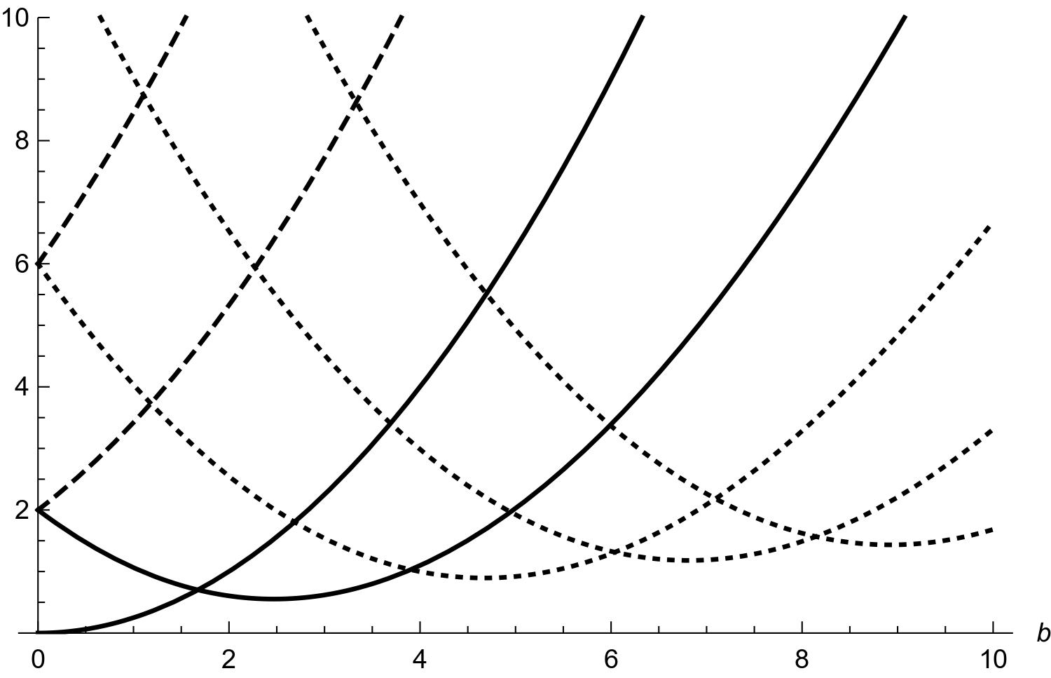
In Figure 1, we see that the crossing between $\lambda_{0}(b)$ and $\lambda_{1}(b)$ occurs on the interval $[0,2]$, and we expect that $\mathfrak{e}(b)$ equals $\lambda_{0}(b)$ or $\lambda_{1}(b)$ on this interval. Because of this, we study the case $0\leq b<2$ in order to check the non-monotonicity.

Let $V_{m,b}(\theta):=\left(\frac{m}{\sin{\theta}}-\frac{b}{2}\right)^{2}$. If $m=0$ then $V_{0,b}(\theta)=\frac{b^{2}}{4}$, and this implies that $\lambda_{0}(b)=\frac{b^{2}}{4}$ (the constant function is an eigenfunction) where $b\geq 0$.

It is sufficient to study the case $m\geq 0$ since for $m\leq-1$ we have that $\lambda_{m}(b)>\frac{b^{2}}{4}$ since $V_{m,b}(\theta)>b^{2}/4$, so

1. (i)

   $0\leq b<1$:

   We note that for $m\geq 1$

   $$\left(\frac{m}{\sin{\theta}}-\frac{b}{2}\right)^{2}=\frac{m}{\sin{\theta}}\left(\frac{m}{\sin{\theta}}-b\right)+\frac{b^{2}}{4}>\frac{b^{2}}{4}.$$

   Hence, $\lambda_{m}(b)>\lambda_{0}(b)$ and $\mathfrak{e}(b)=\lambda_{0}(b)=\frac{b^{2}}{4}.$ Observe that $b\mapsto\mathfrak{e}(b)$ is increasing in this interval.

2. (ii)

   $1\leq b<2$:

   Let $m\geq 2$, then $\frac{m}{\sin{\theta}}\geq 2$ and $b<2$, so

   $$\left(\frac{m}{\sin{\theta}}-\frac{b}{2}\right)^{2}>1>\frac{b^{2}}{4},$$

   so $\mathfrak{e}(b)$ equals $\lambda_{0}(b)$ or $\lambda_{1}(b)$ in this interval.

   Using $g(\theta)=\sin\theta$ as a trial function, one can find a $b_{0}\in[1,2]$ such that $\lambda_{1}(b)<\frac{b^{2}}{4}=\lambda_{0}(b)$ for $b\in(b_{0},2)$. Indeed

   $$\frac{q_{1,b}(g)}{\lVert g\rVert^{2}_{\mathcal{H}}}=\frac{b^{2}}{4}-\frac{3}{8}\pi b+2,$$

   which is smaller than $\lambda_{0}(b)$ for $b>\tfrac{16}{3}\pi\simeq 1.7$. Thus, we have a crossing point.

   Now, we want to increase $b_{0}$ by a small positive amount $\delta>0$ to see $\lambda_{1}(b_{0})>\lambda_{1}(b_{0}+\delta)$. This would mean that we do not have monotonicity. We can rearrange $V_{1,b_{0}+\delta}(\theta)$ as

   $$V_{1,b_{0}+\delta}(\theta)=\left(\frac{1}{\sin{\theta}}-\frac{b_{0}}{2}\right)^{2}+\frac{\delta^{2}}{4}-\delta\left(\frac{1}{\sin{\theta}}-\frac{b_{0}}{2}\right).$$

   Having this in mind, the operator associated with $q_{1,b_{0}+\delta}$ is given by

   (9)

   $$L_{1,b_{0}+\delta}=-\frac{d^{2}}{d\theta^{2}}-\frac{\cos{\theta}}{\sin{\theta}}\frac{d}{d\theta}+V_{1,b_{0}+\delta}(\theta),$$

   Let $f_{0}\in\mathcal{D}(L_{1,b_{0}})$ be a normalized positive eigenfunction of $L_{1,b_{0}}$ with eigenvalue $\lambda_{1}(b_{0})$. Then

   	$\displaystyle q_{1,b_{0}+\delta}(f_{0})$	$\displaystyle=\int_{0}^{\pi}\left(|f_{0}^{\prime}(\theta)|^{2}+V_{1,b_{0}+\delta}(\theta)|f_{0}|^{2}\right)\sin{\theta}\,d\theta$
   		$\displaystyle=q_{1,b_{0}}(f_{0})+\frac{\delta^{2}}{4}-\delta\int_{0}^{\pi}\underbrace{\left(\frac{1}{\sin{\theta}}-\frac{b_{0}}{2}\right)}_{>0}|f_{0}(\theta)|^{2}\sin{\theta}\,d\theta$
   		$\displaystyle=\lambda_{1}(b_{0})-\delta C_{b_{0}}+\frac{\delta^{2}}{4},$

   where $C_{b_{0}}>0$. Thus, for $\delta>0$ small enough we get $\mathfrak{e}(b_{0}+\delta)\leq\lambda_{1}(b_{0}+\delta)<\lambda_{1}(b_{0})=\mathfrak{e}(b_{0})$. We conclude that Theorem 1 holds.

References

- [1] Wafaa Assaad. The breakdown of superconductivity in the presence of magnetic steps. Commun. Contemp. Math., 23(2):Paper No. 2050005, 53, 2021.
- [2] John V. Baxley. The Friedrichs extension of certain singular differential operators. Duke Math. J., 35:455–462, 1968.
- [3] V. Bonnaillie-Noël and S. Fournais. Superconductivity in domains with corners. Rev. Math. Phys., 19(6):607–637, 2007.
- [4] Haim Brezis. Functional analysis, Sobolev spaces and partial differential equations. Universitext. Springer, New York, 2011.
- [5] László Erdős. Dia- and paramagnetism for nonhomogeneous magnetic fields. J. Math. Phys., 38(3):1289–1317, 1997.
- [6] W. Norrie Everitt. A catalogue of Sturm-Liouville differential equations. In Sturm-Liouville theory, pages 271–331. Birkhäuser, Basel, 2005.
- [7] S. Fournais and B. Helffer. On the Ginzburg-Landau critical field in three dimensions. Comm. Pure Appl. Math., 62(2):215–241, 2009.
- [8] Søren Fournais and Bernard Helffer. Strong diamagnetism for general domains and application. volume 57, pages 2389–2400. 2007. Festival Yves Colin de Verdière.
- [9] Søren Fournais and Bernard Helffer. Spectral methods in surface superconductivity, volume 77 of Progress in Nonlinear Differential Equations and their Applications. Birkhäuser Boston, Inc., Boston, MA, 2010.
- [10] Søren Fournais and Mikael Persson. Strong diamagnetism for the ball in three dimensions. Asymptot. Anal., 72(1-2):77–123, 2011.
- [11] Søren Fournais and Mikael Persson Sundqvist. Lack of diamagnetism and the Little-Parks effect. Comm. Math. Phys., 337(1):191–224, 2015.
- [12] Bernard Helffer and Ayman Kachmar. Thin domain limit and counterexamples to strong diamagnetism. Rev. Math. Phys., 33(2):Paper No. 2150003, 35, 2021.
- [13] Bernard Helffer, Ayman Kachmar, and Nicolas Raymond. Magnetic confinement for the 3D Robin Laplacian. Pure Appl. Funct. Anal., 7(2):601–639, 2022.
- [14] Ayman Kachmar and Xing-Bin Pan. Oscillatory patterns in the Ginzburg-Landau model driven by the Aharonov-Bohm potential. J. Funct. Anal., 279(10):108718, 37, 2020.
- [15] Ayman Kachmar and XingBin Pan. Superconductivity and the Aharonov-Bohm effect. C. R. Math. Acad. Sci. Paris, 357(2):216–220, 2019.
- [16] Ayman Kachmar and Mikael P. Sundqvist. Counterexample to strong diamagnetism for the magnetic Robin Laplacian. Math. Phys. Anal. Geom., 23(3):Paper No. 27, 15, 2020.
- [17] W. A. Little and R. D. Parks. Observation of quantum periodicity in the transition temperature of a superconducting cylinder. Phys. Rev. Lett., 9:9–12, Jul 1962.
- [18] Gerald Teschl. Mathematical methods in quantum mechanics, volume 157 of Graduate Studies in Mathematics. American Mathematical Society, Providence, RI, second edition, 2014. With applications to Schrödinger operators.
- [19] Joachim Weidmann. Spectral theory of Sturm-Liouville operators approximation by regular problems. In Sturm-Liouville theory, pages 75–98. Birkhäuser, Basel, 2005.
- [20] Anton Zettl. Sturm-Liouville theory, volume 121 of Mathematical Surveys and Monographs. American Mathematical Society, Providence, RI, 2005.