Equilibrium-nonequilibrium ring-polymer molecular dynamics for nonlinear spectroscopy
Abstract
Two-dimensional Raman and hybrid terahertz-Raman spectroscopic techniques provide invaluable insight into molecular structure and dynamics of condensed-phase systems. However, corroborating experimental results with theory is difficult due to the high computational cost of incorporating quantum-mechanical effects in the simulations. Here, we present the equilibrium-nonequilibrium ring-polymer molecular dynamics (RPMD), a practical computational method that can account for nuclear quantum effects on the two-time response function of nonlinear optical spectroscopy. Unlike a recently developed approach based on the double Kubo transformed (DKT) correlation function, our method is exact in the classical limit, where it reduces to the established equilibrium-nonequilibrium classical molecular dynamics method. Using benchmark model calculations, we demonstrate the advantages of the equilibrium-nonequilibrium RPMD over classical and DKT-based approaches. Importantly, its derivation, which is based on the nonequilibrium RPMD, obviates the need for identifying an appropriate Kubo transformed correlation function and paves the way for applying real-time path-integral techniques to multidimensional spectroscopy.
I Introduction
Two-dimensional vibrational spectroscopy is a versatile technique to study microscopic interactions at their natural, femtosecond time scales.Hamm and Zanni 2011 Recently, a series of hybrid spectroscopic experimentsHamm and Savolainen 2012; Savolainen, Ahmed, and Hamm 2013; Finneran et al. 2016; Grechko et al. 2018 involving mid-infrared, far-infrared (or terahertz), and visible (Raman) pulses have been developed to study electrical and mechanical anharmonicities,Hamm 2014; Finneran et al. 2017; Magdǎu et al. 2019; Mead et al. 2020 structural heterogeneities of liquids,Shalit et al. 2017; Hamm and Shalit 2017; Berger et al. 2019 and the couplings between intermolecular and intramolecular vibrational modes.Ciardi et al. 2019; Vietze et al. 2021 However, the interpretation of such spectra is still an open question and requires adequate simulation methods.Hamm 2019; Berger et al. 2019; Sidler and Hamm 2019; Sidler and Hamm 2020
Several computational methods have been proposed for simulating two-dimensional off-resonant Raman and hybrid terhertz–Raman spectra. Model-based approaches aim at constructing simplified, few-dimensional model systems that can be solved fully quantum mechanically in the presence of a harmonic oscillator bath.Tanimura and Ishizaki 2009; Ikeda, Ito, and Tanimura 2015 These approaches can disentangle contributions to spectra and relate them to different physical effects encoded in the model parameters. The parameters can be obtained by fitting to the existing experimentMagdǎu et al. 2019 or molecular dynamics (MD) simulations.Ueno and Tanimura 2020 Alternatively, MD can be used to simulate spectra directly,Jansen, Snijders, and Duppen 2000; Jansen, Snijders, and Duppen 2001; Saito and Ohmine 2002; Saito and Ohmine 2003; DeVane et al. 2003; Hasegawa and Tanimura 2006; Hasegawa and Tanimura 2008; Yagasaki and Saito 2009; Ito, Hasegawa, and Tanimura 2014; Hamm 2014; Sun 2019; Jansen et al. 2019 as a way to cross-validate the simplified model and further test the molecular mechanics force field or ab initio quantum chemistry method used for describing the forces between atoms, dipole moments, and polarizabilities.Hasegawa and Tanimura 2011; Ito, Hasegawa, and Tanimura 2016; Sidler, Meuwly, and Hamm 2018 However, one improvement of MD is highly desired—MD simulations are based on classical atomic nuclei and neglect nuclear quantum effects, which can significantly modify the spectra. Indeed, recent two-dimensional Raman–THz–THz spectra of H2O and D2O revealed the effect of isotopic substitution beyond what would be expected from classical mechanics, pointing at nuclear quantum effects of the light hydrogen atoms.Berger et al. 2019
Quantum simulations of the condensed phase have been enabled by various semiclassical methods based on the classical MD framework, including linearized semiclassical initial value representation (LSC-IVR),Wang, Sun, and Miller 1998; Liu and Miller 2006 path-integral Liouville dynamics,Liu 2014 centroid molecular dynamics (CMD),Jang and Voth 1999 and ring-polymer molecular dynamics (RPMD).Craig and Manolopoulos 2004 These methods have proven useful for the computation of one-time correlation functionsHabershon et al. 2013 related to various dynamical properties, including reaction rates,Wang, Sun, and Miller 1998; Jang and Voth 2000; Boekelheide, Salomón-Ferrer, and Miller 2011; Suleimanov, Javier Aoiz, and Guo 2016; Tao, Shushkov, and Miller 2019; Tao, Shushkov, and Miller 2020 diffusion coefficients,Miller and Manolopoulos 2005a; Miller and Manolopoulos 2005b and one-dimensional vibrational spectra.Witt et al. 2009; Rossi, Ceriotti, and Manolopoulos 2014; Benson, Trenins, and Althorpe 2019; Trenins, Willatt, and Althorpe 2019; Korol et al. 2020; Rosa-Raíces et al. 2021 Some of them have also been applied to two-dimensional electronicLoring 2017; Polley and Loring 2020; Provazza et al. 2018; Provazza, Segatta, and Coker 2020; Gao and Geva 2020 and infrared spectroscopies,Gruenbaum and Loring 2009; Gerace and Loring 2013; Alemi and Loring 2015; Kwac and Geva 2013 in which the quantum subsystem, consisting of, e.g., electronic or high-frequency vibrational degrees of freedom, can be well defined.Shi and Geva 2008; McRobbie et al. 2009; McRobbie and Geva 2009 In contrast, their application to two-dimensional Raman and hybrid terahertz-Raman spectroscopic techniques, in which all vibrational degrees of freedom should be treated on an equal footing, has been limited. Recently, the group of BatistaJung, Videla, and Batista 2018; Jung, Videla, and Batista 2019; Jung, Videla, and Batista 2020 proposed a set of methods that approximate the symmetric contribution to the so-called double Kubo transformed (DKT) correlation function, which is a two-time extension of the original one-time Kubo transformed correlation function.Habershon et al. 2013 However, the relation between the symmetrized DKT correlation function and the spectroscopic response function is only approximate.
Here, we present an alternative RPMD approach to two-dimensional spectroscopy, which directly considers the two-time response function and does not rely on the additional approximation related to the DKT correlation function. To derive the proposed method, we start from the recently developed nonequilibrium RPMDWelsch et al. 2016; Marjollet and Welsch 2020; Marjollet and Welsch 2021; Jiang et al. 2021; Marjollet, Inhester, and Welsch 2022 and employ classical response theory. We then explore its validity and limitations both theoretically and numerically.
II Theory
In two-dimensional RamanTanimura and Mukamel 1993; Palese et al. 1994 and hybrid terahertz-Raman spectroscopies,Savolainen, Ahmed, and Hamm 2013; Finneran et al. 2016; Grechko et al. 2018 the signal is measured as a function of two delay times between three ultrashort light pulses, whose specific sequence determines the type of spectroscopy. To keep the discussion general, we consider the time-dependent Hamiltonian
| (1) |
comprised of the system’s field-free Hamiltonian and two interactions with the first two ultrashort pulses, controlled, respectively, by coordinate-dependent operators and and by time-dependent functions representing the pulse shapes. For terahertz pulses, the interaction operators are the system’s dipole moments and functions are the electric fields of the light, whereas for the visible/near-infrared (Raman) pulses or sum-frequency terahertz excitation,Mead et al. 2020 the operators are the system’s polarizabilities and the time-dependent functions correspond to the squares of the electric fields. is centered at , is centered at , and the signal is measured at , where and represent the time delays between the three light pulses. The recorded signal is proportional to the expectation valueFinneran et al. 2017
| (2) |
of another coordinate-dependent operator , which is again either the polarizability or dipole moment operator of the system. In Eq. (2), system’s equilibrium density operator evolves under the time-dependent Hamiltonian (1), i.e.,
| (3) | |||||
| (4) |
is the inverse temperature, and is the time ordering operator. In practice, the experiments are designed to extract the components of the signal that are proportional to and , which can be accounted for by evaluating the signal asMagdǎu et al. 2019
| (5) |
where represents the expectation value (2) of the system evolved under the Hamiltonian (1) with and . For sufficiently weak external fields, we can further invoke second-order time-dependent perturbation theory and recover the well-known resultTanimura and Mukamel 1993
| (6) |
where
| (7) |
is the corresponding response function, which depends only on the system’s properties. Because it can be easily convolved with different experimental pulses to recover the observed experimental signals (6), the response function is often the direct target of many theoretical studies. Here, we also intend to focus on the response function, but take a slightly different route in developing the computational approach. Namely, we note that for delta pulses, and , the signal measured after the second time delay is proportional to the response function,
| (8) |
where control the amplitude of the external fields. In the following, we derive an approximation to under weak delta pulses and relate it to using Eq. (8).
To develop a tractable theory for condensed-phase simulations of spectra, we replace the exact quantum-mechanical expression (2) by its nonequilibrium RPMDWelsch et al. 2016 approximation
| (9) |
where and are the positions and momenta of the extended system comprised of replicas of the original -dimensional system,
| (10) |
is the corresponding phase-space distribution,
| (11) |
is the system’s field-free ring-polymer Hamiltonian,Habershon et al. 2013 ,
| (12) |
is the symmetric mass matrix of the system, and . The classical time evolution of and is governed by the time-dependent ring-polymer Hamiltonian
| (13) | |||
| (14) |
with . Nonequilibrium RPMD, in which the dynamics and initial distribution depend on different Hamiltonians [see Eqs. (9)–(11) and (13)], has been rigorously justified as an approximation to the more general real-time nonequilibrium Matsubara dynamics.Welsch et al. 2016 Although its original derivation involved only time-independent Hamiltonians, this assumption was not used explicitly at any step of the derivation, justifying the use of nonequilibrium RPMD even in the time-dependent setting. At this point, we recognize that the equations above already formulate a valid computational technique for evaluating the response function, which, in the limit of , is equivalent to the finite-field nonequilibrium MD method of Jansen, Snijders, and Duppen.Jansen, Snijders, and Duppen 2000; Jansen, Snijders, and Duppen 2001 In contrast to their classical approach, the nonequilibrium RPMD theory can include, at least approximately, the nuclear quantum effects on two-dimensional spectra when the path-integral continuum limit is reached. However, these nonequilibrium (RP)MD methods are impractical because a different set of trajectories is needed for each choice of the delay time . To address this problem, we employ the equilibrium-nonequilibrium approach, originally developed by Hasegawa and TanimuraHasegawa and Tanimura 2006 in the context of classical MD simulations, in which one of the two pulses is treated perturbatively, and combine it with the RPMD to account for nuclear quantum effects.
We start by rewriting Eq. (9) as
| (15) |
where
| (16) |
governs the time evolution under the Hamiltonian ,
| (17) |
is the corresponding Liouvillian, , , , and denotes the Poisson bracket. Next, we expandHolian and Evans 1985; Plé et al. 2021
| (18) | |||||
| (19) |
to the first order in to obtain
| (20) |
where
| (21) |
and
| (22) |
In Eq. (18) we introduced a short-hand notation
| (23) |
for the evolution operator that involves only the second pulse. In going from Eq. (18) to Eq. (19), we assumed that and used
| (24) |
with
| (25) |
Then, we derive
| (26) |
from Eq. (22) by applying ,
| (27) | |||||
| (28) | |||||
| (29) |
where denotes the time derivative, and Eq. (24) in combination with and . is the position along a backward equilibrium trajectory. corresponds to a nonequilibrium trajectory evolved under the Hamiltonian that involves the interaction with the second pulse, which is equivalent to the field-free evolution with the initial conditions and .
Combining Eq. (26) with Eqs. (5), (8), and (20) yields the final result
| (30) |
assuming is sufficiently small to guarantee the validity of the perturbative expression (8). It follows that the response function can be evaluated as an equilibrium ensemble average of an estimator based on two nonequilibrium trajectories () and one backward equilibrium trajectory (). At high temperatures, where , or for , Eq. (30) reduces to the equilibrium-nonequilibrium classical MD approach.Hasegawa and Tanimura 2006 In contrast to the classical approach, the RPMD method captures nuclear quantum effects, in accordance with the well-known advantages and limitations of the RPMD for one-time correlation functions.Habershon et al. 2013 Furthermore, in the Supplementary Material, we show that the RPMD is exact for the harmonic oscillator when two out of three operators , , and are linear functions of position. Finally, the proposed equilibrium-nonequilibrium RPMD method always satisfies (because ), which holds for the exact quantum response function (7), but is not guaranteed by some other approximate methods (as discussed below).
Before demonstrating these properties numerically, we briefly review the only other RPMD-based method proposed to date for simulating two-dimensional vibrational spectra. In 2018, Jung, Videla, and BatistaJung, Videla, and Batista 2018 showed that the response function (7) is related to the DKT correlation function,Tong et al. 2020
| (31) |
through the frequency-domain expression
| (32) |
where
| (33) | |||
| (34) |
and are some known functions of and .Tong et al. 2020 Although Eq. (32) is exact, an additional approximation is needed before can be evaluated using the RPMD. Specifically, the authors employed the symmetrized DKT approximation
| (35) |
neglecting the asymmetric contribution to the DKT correlation function, to make use of the RPMD approximation
| (36) |
Thus, the symmetrized DKT approximation, and as a consequence the RPMD DKT method as well, is not exact in the classical limit. In addition, the corresponding response functions need not be zero at ,Tong et al. 2020 except in the high-temperature limit, in which case the RPMD DKT method reduces to the classical correlation function approach of DeVane, Ridley, Space, and Keyes.DeVane et al. 2003; DeVane et al. 2004; DeVane et al. 2005; DeVane et al. 2006
III Results and discussion
In this Section, the above considerations about the classical, RPMD, and RPMD DKT methods for simulating two-dimensional vibrational spectra are demonstrated numerically on an anharmonic model system determined by the Hamiltonian
| (37) |
where is a tunable parameter that controls the degree of anharmonicity. This system can be solved numerically exactly in a finite basis and was previously used with to evaluate the accuracy of RPMD and nonequilibrium RPMD methods.Craig and Manolopoulos 2004; Welsch et al. 2016 Details of the exact quantum and approximate trajectory-based simulations can be found in the Supplementary Material.
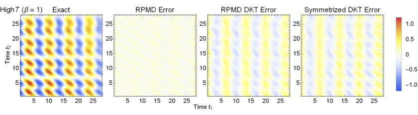
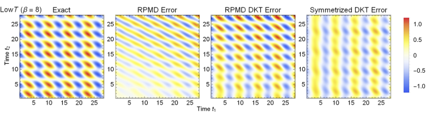
Figure 1 shows that the equilibrium-nonequilibrium RPMD approach performs better than the RPMD DKT method at both low and high temperatures. Notably, the newly proposed RPMD approach exhibits the expected short-time accuracy, while most of the error in the RPMD DKT method can be attributed to the neglect of the asymmetric part of the full DKT correlation function (compare columns 3 and 4 of Fig. 1).
Figure 2 shows the time slices of along (left panels) and (right panels). At low temperature (Fig. 2, bottom), equilibrium-nonequilibrium RPMD is more accurate than the classical method due to the inclusion of nuclear quantum effects, while the two are similar at high temperature (Fig. 2, top). Although the RPMD response function agrees with the exact result at short time (see Fig. 2, bottom left), its long-time oscillation frequency deviates from the exact, because RPMD is not expected to recover quantum coherence effects. In this example, the classical simulation is more accurate than the RPMD DKT method, showing that the uncontrolled error of the symmetrized DKT approximation can outweigh the benefits of including nuclear quantum effects. In fact, similar findings were implied, even if not explicitly discussed, by the earlier reports on the symmetrized DKT approximation.Jung, Videla, and Batista 2018; Tong et al. 2020 In addition, both classical and RPMD equilibrium-nonequilibrium methods are exact (zero) at (see left panels of Fig. 2), which does not hold for the RPMD DKT approach (see also Figs. 6e and 8e of Ref. Tong et al. 2020).
To demonstrate numerically that the proposed approach inherits some well-known properties of RPMD, we choose to quantify the error of an approximate response function as
| (38) |
where and is the exact response function. Figure 3 shows that the equilibrium-nonequilibrium RPMD consistently outperforms the classical approach for systems of different anharmonicities (a), at different temperatures (b), and for different combinations of operators (c). As discussed earlier, the RPMD method is exact for the harmonic oscillator (, see Fig. 3a) and certain combinations of operators , , and . Interestingly, the classical approach is also exact in some of those limiting cases (see Supplementary Material). Nevertheless, as soon as the system is even weakly anharmonic, RPMD is clearly superior to the classical approach. As expected, both RPMD and classical methods perform worse as the anharmonicity increases. Furthermore, the equilibrium-nonequilibrium RPMD method converges to the exact (classical) result in the high-temperature limit (, Fig.3b). Again, as the temperature decreases, the RPMD approach becomes less accurate. Finally, the proposed RPMD approach is more accurate for linear compared to nonlinear operators (Fig. 3c).
We further consider a two-dimensional model Hamiltonian
| (39) |
composed of two anharmonic oscillators [Eq. (37), ] with different central frequencies (, ) and a linear-linear coupling term proportional to . The light-matter interaction operators are set to , , reflecting the terahertz-infrared-Raman pulse sequence,Grechko et al. 2018; Vietze et al. 2021 in which the first, terahertz pulse interacts only with the low-frequency mode , while the infrared and off-resonant Raman interactions probe the high-frequency mode . Figure 4 shows that the two-dimensional spectrum, obtained as the double cosine transform of the two-time response function (see Supplementary Material for further details), exhibits off-diagonal peaks at and , as predicted by the Feynman diagrams of Refs. Sidler and Hamm 2020; Vietze et al. 2021. The signal vanishes in the absence of coupling, , or anharmonicity, (see Section III of the Supplementary Material). Equilibrium-nonequilbrium RPMD and classical MD spectra reproduce the shape of the exact spectrum. However, at low temperature (Fig. 4, bottom), classical method largely overestimates the magnitudes of the off-diagonal peaks due to the neglect of the nuclear quantum effects. In our simplified case, this results mostly in an overall scaling factor, but, in general, could affect the relative intensities of the spectral features.

IV Conclusion
To conclude, we have introduced an RPMD-based method that captures nuclear quantum effects on three-pulse two-dimensional vibrational spectra at the cost of classical MD simulations. The proposed approach was shown to perform better than the classical and recently developed RPMD DKT methods. Although our discussion focused only on RPMD, the overall scheme could be extended to the more general Matsubara dynamicsHele et al. 2015a; Hele et al. 2015b; Hele 2017 and to its efficient approximations, including thermostated RPMD,Rossi, Ceriotti, and Manolopoulos 2014 CMD,Jang and Voth 1999 and quasi-CMD.Trenins, Willatt, and Althorpe 2019 It would be interesting to see how these approximations perform when applied to multidimensional spectroscopy, because it is expected to provide a more stringent test for dynamical approximations compared to linear spectroscopy, for which similar studies exist.Benson, Trenins, and Althorpe 2019 Because two-dimensional Raman and hybrid THz–Raman spectra vanish for harmonic potentials with linear dipole moment or polarizability operators,Tanimura and Mukamel 1993 adequate computational approaches must capture the effect of electrical and mechanical anharmonicities, which poses a challenge for RPMD and the above-mentioned methods.Plé et al. 2021; Benson and Althorpe 2021
To derive the equilibrium-nonequilibrium RPMD, we did not invoke the concept of the Kubo transformation, which is traditionally done for one-time correlation functions,Habershon et al. 2013 but instead combined nonequilibrium RPMD with classical response theory. This new way of deriving real-time path-integral methods will be of special interest for simulating time-resolved spectroscopic experiments, but also in other contexts where multi-time correlation or response functions appear, or if a derivation of the appropriate Kubo transformed correlation function is not obvious. The theory is general and enables new applications of established quantum dynamical methods.
Supplementary material
See the supplementary material for the computational details, analytical expressions in the harmonic limit, and further discussion of the two-mode system in the absence of coupling or anharmonicity.
Acknowledgements.
The authors thank Kenneth A. Jung, Roman Korol, and Jorge L. Rosa-Raíces for helpful discussions. TB acknowledges financial support from the Swiss National Science Foundation through the Early Postdoc Mobility Fellowship (grant number P2ELP2-199757). GAB and TFM gratefully acknowledge support from the National Science Foundation Chemical Structure, Dynamics and Mechanisms program (grant CHE-1665467). The computations presented here were conducted in the Resnick High Performance Computing Center, a facility supported by Resnick Sustainability Institute at the California Institute of Technology.Data availability
The data that support the findings of this study are available from the corresponding author upon reasonable request.
References
- Hamm and Zanni (2011) P. Hamm and M. Zanni, Concepts and Methods of 2D Infrared Spectroscopy (Cambridge University Press, 2011).
- Hamm and Savolainen (2012) P. Hamm and J. Savolainen, J. Chem. Phys. 136, 094516 (2012).
- Savolainen, Ahmed, and Hamm (2013) J. Savolainen, S. Ahmed, and P. Hamm, Proc. Nat. Acad. Sci. USA 110, 20402 (2013).
- Finneran et al. (2016) I. A. Finneran, R. Welsch, M. A. Allodi, T. F. Miller, and G. A. Blake, Proc. Nat. Acad. Sci. USA 113, 6857 (2016).
- Grechko et al. (2018) M. Grechko, T. Hasegawa, F. D’Angelo, H. Ito, D. Turchinovich, Y. Nagata, and M. Bonn, Nat. Commun. 9, 885 (2018).
- Hamm (2014) P. Hamm, J. Chem. Phys. 141, 184201 (2014).
- Finneran et al. (2017) I. A. Finneran, R. Welsch, M. A. Allodi, T. F. Miller, and G. A. Blake, J. Phys. Chem. Lett. 8, 4640 (2017).
- Magdǎu et al. (2019) I. B. Magdǎu, G. J. Mead, G. A. Blake, and T. F. Miller, J. Phys. Chem. A 123, 7278 (2019).
- Mead et al. (2020) G. Mead, H. W. Lin, I. B. Magdǎu, T. F. Miller, and G. A. Blake, J. Phys. Chem. B 124, 8904 (2020).
- Shalit et al. (2017) A. Shalit, S. Ahmed, J. Savolainen, and P. Hamm, Nat. Chem. 9, 273 (2017).
- Hamm and Shalit (2017) P. Hamm and A. Shalit, J. Chem. Phys. 146, 130901 (2017).
- Berger et al. (2019) A. Berger, G. Ciardi, D. Sidler, P. Hamm, and A. Shalit, Proc. Nat. Acad. Sci. USA 116, 2458 (2019).
- Ciardi et al. (2019) G. Ciardi, A. Berger, P. Hamm, and A. Shalit, J. Phys. Chem. Lett. 10, 4463 (2019).
- Vietze et al. (2021) L. Vietze, E. H. G. Backus, M. Bonn, and M. Grechko, J. Chem. Phys. 154, 174201 (2021).
- Hamm (2019) P. Hamm, J. Chem. Phys. 151, 054505 (2019).
- Sidler and Hamm (2019) D. Sidler and P. Hamm, J. Chem. Phys. 150, 044202 (2019).
- Sidler and Hamm (2020) D. Sidler and P. Hamm, J. Chem. Phys. 153, 044502 (2020).
- Tanimura and Ishizaki (2009) Y. Tanimura and A. Ishizaki, Acc. Chem. Res. 42, 1270 (2009).
- Ikeda, Ito, and Tanimura (2015) T. Ikeda, H. Ito, and Y. Tanimura, J. Chem. Phys. 142, 212421 (2015).
- Ueno and Tanimura (2020) S. Ueno and Y. Tanimura, J. Chem. Theory Comput. 16, 2099 (2020).
- Jansen, Snijders, and Duppen (2000) T. l. C. Jansen, J. G. Snijders, and K. Duppen, J. Chem. Phys. 113, 307 (2000).
- Jansen, Snijders, and Duppen (2001) T. l. C. Jansen, J. G. Snijders, and K. Duppen, J. Chem. Phys. 114, 10910 (2001).
- Saito and Ohmine (2002) S. Saito and I. Ohmine, Phys. Rev. Lett. 88, 207401 (2002).
- Saito and Ohmine (2003) S. Saito and I. Ohmine, J. Chem. Phys. 119, 9073 (2003).
- DeVane et al. (2003) R. DeVane, C. Ridley, B. Space, and T. Keyes, J. Chem. Phys. 119, 6073 (2003).
- Hasegawa and Tanimura (2006) T. Hasegawa and Y. Tanimura, J. Chem. Phys. 125, 074512 (2006).
- Hasegawa and Tanimura (2008) T. Hasegawa and Y. Tanimura, J. Chem. Phys. 128, 064511 (2008).
- Yagasaki and Saito (2009) T. Yagasaki and S. Saito, Acc. Chem. Res. 42, 1250 (2009).
- Ito, Hasegawa, and Tanimura (2014) H. Ito, T. Hasegawa, and Y. Tanimura, J. Chem. Phys. 141, 124503 (2014).
- Sun (2019) X. Sun, J. Chem. Phys. 151, 194507 (2019).
- Jansen et al. (2019) T. L. C. Jansen, S. Saito, J. Jeon, and M. Cho, J. Chem. Phys. 150, 100901 (2019).
- Hasegawa and Tanimura (2011) T. Hasegawa and Y. Tanimura, J. Phys. Chem. B 115, 5545 (2011).
- Ito, Hasegawa, and Tanimura (2016) H. Ito, T. Hasegawa, and Y. Tanimura, J. Phys. Chem. Lett. 7, 4147 (2016).
- Sidler, Meuwly, and Hamm (2018) D. Sidler, M. Meuwly, and P. Hamm, J. Chem. Phys. 148, 244504 (2018).
- Wang, Sun, and Miller (1998) H. Wang, X. Sun, and W. H. Miller, J. Chem. Phys. 108, 9726 (1998).
- Liu and Miller (2006) J. Liu and W. H. Miller, J. Chem. Phys. 125, 224104 (2006).
- Liu (2014) J. Liu, J. Chem. Phys. 140, 224107 (2014).
- Jang and Voth (1999) S. Jang and G. A. Voth, J. Chem. Phys. 111, 2371 (1999).
- Craig and Manolopoulos (2004) I. R. Craig and D. E. Manolopoulos, J. Chem. Phys. 121, 3368 (2004).
- Habershon et al. (2013) S. Habershon, D. E. Manolopoulos, T. E. Markland, and T. F. Miller, Annu. Rev. Phys. Chem. 64, 387 (2013).
- Jang and Voth (2000) S. Jang and G. A. Voth, J. Chem. Phys. 112, 8747 (2000).
- Boekelheide, Salomón-Ferrer, and Miller (2011) N. Boekelheide, R. Salomón-Ferrer, and T. F. Miller, Proc. Nat. Acad. Sci. USA 108, 16159 (2011).
- Suleimanov, Javier Aoiz, and Guo (2016) Y. V. Suleimanov, F. Javier Aoiz, and H. Guo, J. Phys. Chem. A 120, 8488 (2016).
- Tao, Shushkov, and Miller (2019) X. Tao, P. Shushkov, and T. F. Miller, J. Phys. Chem. A 123, 3013 (2019).
- Tao, Shushkov, and Miller (2020) X. Tao, P. Shushkov, and T. F. Miller, J. Chem. Phys. 152, 124117 (2020).
- Miller and Manolopoulos (2005a) T. F. Miller and D. E. Manolopoulos, J. Chem. Phys. 122, 184503 (2005a).
- Miller and Manolopoulos (2005b) T. F. Miller and D. E. Manolopoulos, J. Chem. Phys. 123, 154504 (2005b).
- Witt et al. (2009) A. Witt, S. D. Ivanov, M. Shiga, H. Forbert, and D. Marx, J. Chem. Phys. 130, 194510 (2009).
- Rossi, Ceriotti, and Manolopoulos (2014) M. Rossi, M. Ceriotti, and D. E. Manolopoulos, J. Chem. Phys. 140, 234116 (2014).
- Benson, Trenins, and Althorpe (2019) R. L. Benson, G. Trenins, and S. C. Althorpe, Faraday Discuss. 221, 350 (2019).
- Trenins, Willatt, and Althorpe (2019) G. Trenins, M. J. Willatt, and S. C. Althorpe, J. Chem. Phys. 151, 054109 (2019).
- Korol et al. (2020) R. Korol, J. L. Rosa-Raíces, N. Bou-Rabee, and T. F. Miller, J. Chem. Phys. 152, 104102 (2020).
- Rosa-Raíces et al. (2021) J. L. Rosa-Raíces, J. Sun, N. Bou-Rabee, and T. F. Miller, J. Chem. Phys. 154, 024106 (2021).
- Loring (2017) R. F. Loring, J. Chem. Phys. 146, 144106 (2017).
- Polley and Loring (2020) K. Polley and R. F. Loring, J. Phys. Chem. B 124, 9913 (2020).
- Provazza et al. (2018) J. Provazza, F. Segatta, M. Garavelli, and D. F. Coker, J. Chem. Theory Comput. 14, 856 (2018).
- Provazza, Segatta, and Coker (2020) J. Provazza, F. Segatta, and D. F. Coker, J. Chem. Theory Comput. 17, 29 (2020).
- Gao and Geva (2020) X. Gao and E. Geva, J. Chem. Theory Comput. 16, 6491 (2020).
- Gruenbaum and Loring (2009) S. M. Gruenbaum and R. F. Loring, J. Chem. Phys. 131, 204504 (2009).
- Gerace and Loring (2013) M. Gerace and R. F. Loring, J. Chem. Phys. 138, 124104 (2013).
- Alemi and Loring (2015) M. Alemi and R. F. Loring, J. Chem. Phys. 142, 212417 (2015).
- Kwac and Geva (2013) K. Kwac and E. Geva, J. Phys. Chem. B 117, 7737 (2013).
- Shi and Geva (2008) Q. Shi and E. Geva, J. Chem. Phys. 129, 124505 (2008).
- McRobbie et al. (2009) P. L. McRobbie, G. Hanna, Q. Shi, and E. Geva, Acc. Chem. Res. 42, 1299 (2009).
- McRobbie and Geva (2009) P. L. McRobbie and E. Geva, J. Phys. Chem. A 113, 10425 (2009).
- Jung, Videla, and Batista (2018) K. A. Jung, P. E. Videla, and V. S. Batista, J. Chem. Phys. 148, 244105 (2018).
- Jung, Videla, and Batista (2019) K. A. Jung, P. E. Videla, and V. S. Batista, J. Chem. Phys. 151, 034108 (2019).
- Jung, Videla, and Batista (2020) K. A. Jung, P. E. Videla, and V. S. Batista, J. Chem. Phys. 153, 124112 (2020).
- Welsch et al. (2016) R. Welsch, K. Song, Q. Shi, S. C. Althorpe, and T. F. Miller, J. Chem. Phys. 145, 204118 (2016).
- Marjollet and Welsch (2020) A. Marjollet and R. Welsch, J. Chem. Phys. 152, 194113 (2020).
- Marjollet and Welsch (2021) A. Marjollet and R. Welsch, Int. J. Quant. Chem. 121, e26447 (2021).
- Jiang et al. (2021) H. Jiang, X. Tao, M. Kammler, F. Ding, A. M. Wodtke, A. Kandratsenka, T. F. Miller, and O. Bünermann, J. Phys. Chem. Lett. 12, 1991 (2021).
- Marjollet, Inhester, and Welsch (2022) A. Marjollet, L. Inhester, and R. Welsch, J. Chem. Phys. 156, 044101 (2022).
- Tanimura and Mukamel (1993) Y. Tanimura and S. Mukamel, J. Chem. Phys. 99, 9496 (1993).
- Palese et al. (1994) S. Palese, J. T. Buontempo, L. Schilling, W. T. Lotshaw, Y. Tanimura, S. Mukamel, and R. J. D. Miller, J. Phys. C 98, 12466 (1994).
- Holian and Evans (1985) B. L. Holian and D. J. Evans, J. Chem. Phys. 83, 3560 (1985).
- Plé et al. (2021) T. Plé, S. Huppert, F. Finocchi, P. Depondt, and S. Bonella, J. Chem. Phys. 155, 104108 (2021).
- Tong et al. (2020) Z. Tong, P. E. Videla, K. A. Jung, V. S. Batista, and X. Sun, J. Chem. Phys. 153, 034117 (2020).
- DeVane et al. (2004) R. DeVane, C. Ridley, B. Space, and T. Keyes, Phys. Rev. E 70, 050101(R) (2004).
- DeVane et al. (2005) R. DeVane, C. Ridley, B. Space, and T. Keyes, J. Chem. Phys. 123, 194507 (2005).
- DeVane et al. (2006) R. DeVane, C. Kasprzyk, B. Space, and T. Keyes, J. Phys. Chem. B 110, 3773 (2006).
- Hele et al. (2015a) T. J. H. Hele, M. J. Willatt, A. Muolo, and S. C. Althorpe, J. Chem. Phys. 142, 134103 (2015a).
- Hele et al. (2015b) T. J. H. Hele, M. J. Willatt, A. Muolo, and S. C. Althorpe, J. Chem. Phys. 142, 191101 (2015b).
- Hele (2017) T. J. H. Hele, Mol. Phys. 115, 1435 (2017).
- Benson and Althorpe (2021) R. L. Benson and S. C. Althorpe, J. Chem. Phys. 155, 104107 (2021).