The Role of Linear Layers in Nonlinear Interpolating Networks

Past work has explored the role of neural network depth via a “depth separation” analysis (e.g. Daniely, 2017; Vardi and Shamir, 2020); these analyses identify functions which may be efficiently represented at one depth but require an exponential width to represent them with fewer layers. This line of work has yielded important insights into the role of depth, but recent work has highlighted how functions leading to depth separation results are often highly oscillatory and perhaps not fully capturing the import of depth in practical settings (i.e., may be “worse case” but not “average case” results). In particular, Safran et al., 2019 shows that if the Lipschitz constant of the target function is kept fixed, then existing depth separation results between 2- and 3-layer nets do not hold.

A number of papers have studied representation costs and implicit regularization from a function space perspective associated with neural networks. Following a univariate analysis by Savarese et al., 2019, Ongie et al., 2019 considers two-layer multivariate ReLU networks where the hidden layer has infinite width:

$$\lim_{K\rightarrow\infty}\sum_{k=1}^{K}a_{k}[{\bm{w}}_{k}^{\top}{\bm{x}}+b_{k}]_{+}.$$

Recent work by Mulayoff et al., 2021 connects the function space representation costs of two-layer ReLU networks to the stability of SGD minimizers.

Gunasekar et al., 2018 shows that $L$-layer linear networks with diagonal structure induces a non-convex implicit bias over network weights corresponding to the $\ell^{q}$ norm of the outer layer weights for $q=2/L$; similar conclusions hold for deep linear convolutional networks. Recent work by Dai et al., 2021 examines the representation costs of deep linear networks from a function space perspective. However, the existing literature does not fully characterize the representation costs of deep, non-linear networks from a function space perspective. Parhi and Nowak, 2021 consider deeper networks and define a compositional function space with a corresponding representor theorem; the properties of this function space and the role of depth are an area of active investigation.

Our paper focuses on the role of linear layers in nonlinear networks. The role of linear layers in such settings has been explored in a number of works. Golubeva et al., 2020 looks at the role of network width when the number of parameters is held fixed; it specifically looks at increasing the width without increasing the number of parameters by adding linear layers. This procedure seems to help with generalization performance (as long as the training error is controlled). However, Golubeva et al., 2020 note that the implicit regularization caused by this approach is not understood. One of the main contributions of our paper is a better understanding of this implicit regularization.

The effect of linear layers on training speed was previously examined by Ba and Caruana, 2013; Urban et al., 2016. Arora et al., 2018 considers implicit acceleration in deep nets and claims that depth induce a momentum-like term in training deep linear networks with SGD, though the regularization effects of this acceleration are not well understood. Implicit regularization of gradient descent has been studied in the context of matrix and tensor factorization problems Gunasekar et al., 2018; Arora et al., 2019; Razin and Cohen, 2020; Razin et al., 2021. Similar to this work, low-rank representations play a key role in their analysis.

For a vector ${\bm{a}}\in\mathbb{R}^{K}$, we use $\|{\bm{a}}\|_{p}$ to denote its $\ell^{p}$ norm. For a matrix ${\bm{W}}$, we use $\|{\bm{W}}\|_{F}$ to denote the Frobenius norm, $\|{\bm{W}}\|_{*}$ to denote its nuclear norm (i.e., the sum of the singular values), and for $0<q\leq 1$ we use $\|{\bm{W}}\|_{\mathcal{S}^{q}}$ to denote its Schatten-$q$ quasi-norm (i.e., the $\ell^{q}$ quasi-norm of the singular values of a matrix ${\bm{W}}$). Given a vector ${\bm{a}}\in\mathbb{R}^{K}$, the matrix ${\bm{D}}_{{\bm{a}}}\in\mathbb{R}^{K\times K}$ is a diagonal matrix with the entries of ${\bm{a}}$ along the diagonal. For a vector $\bm{\lambda}$, we write $\bm{\lambda}>0$ to indicate it has all positive entries. Finally, we use $[t]_{+}=\max\{0,t\}$ to denote the ReLU activation, and whose application to vectors is understood entrywise.

We prove that in the special case where the training features are entirely contained in a subspace, every minimum $R_{L}$-cost interpolating solution must depend on only the projection of features onto that subspace:

More generally, since the representation cost is translation invariant, the above result extends to the case where the training features span an affine subspace $\mathcal{A}:=\{{\bm{v}}+{\bm{x}}:{\bm{x}}\in\mathcal{S}\}$ where ${\bm{v}}\in\mathcal{S}^{\perp}$, in which case we have $f({\bm{x}})=f({\bm{P}}_{\mathcal{S}}{\bm{x}}+{\bm{v}})$.

The above proposition implies that any minimum $R_{L}$-cost interpolant $f$ will have all its units aligned with ${\cal S}$; i.e., every inner-layer weight vector ${\bm{w}}_{k}\in{\cal S}\;\forall\;k$. Thus, $f$ will be constant in directions orthogonal to ${\cal S}$.

Specializing this result to the case of training features constrained to a one-dimensional subspace, we see that all minimum $R_{L}$-cost interpolants must have units aligned along the subspace (rank-one inner-layer weight matrix). Combined with Corollary 3.6, this gives the immediate corollary:

The above results do not depend on the number of linear layers. However, next we show there are settings where minimum $R_{L}$-cost interpolating solutions differ for $L=2$ and $L=3$.

Suppose that training samples may be interpolated by a function

$\displaystyle f_{*}({\bm{x}})=$

$\displaystyle\sum_{k=1}^{K}a_{k}[{\bm{w}}_{k}^{\top}{\bm{x}}+b_{k}]_{+}+c,$

(20)

and assume that $\|{\bm{w}}_{k}\|=1\;\forall\;k$. Given a subspace ${\cal S}$ and corresponding orthogonal projection operator ${\bm{P}}_{\cal S}$ where ${\bm{P}}_{\cal S}{\bm{w}}_{k}\neq 0\;\forall\;k$, we construct the function

$\displaystyle g_{\cal S}({\bm{x}})=$

$\displaystyle\sum_{k=1}^{K}\tilde{a}_{k}[\tilde{\bm{w}}_{k}^{\top}{\bm{x}}+\tilde{b}_{k}]_{+}+c$

(21)

where

$\displaystyle\tilde{\bm{w}}_{k}:=\frac{{\bm{P}}_{\cal S}{\bm{w}}_{k}}{\|{\bm{P}}_{\cal S}{\bm{w}}_{k}\|_{2}},\qquad\tilde{a}_{k}:=\frac{a_{k}}{r_{k}},\qquad\tilde{b}_{k}:=\frac{b_{k}a_{k}}{\tilde{a}_{k}},$

(22)

and $r_{k}$ is defined as follows. Let ${\bm{X}}_{k}\in\mathbb{R}^{d\times n_{k}}$ be a matrix of the $n_{k}\leq n$ training samples that are “active” under ReLU unit $k$ – that is, ${\bm{x}}_{i}$ is a column of ${\bm{X}}_{k}$ if ${\bm{w}}_{k}^{\top}{\bm{x}}_{i}+b_{k}>0$. Further define $\Sigma_{k}:={\bm{X}}_{k}{\bm{X}}_{k}^{\top}$. Then we define

$\displaystyle r_{k}:=\frac{{\bm{w}}_{k}^{\top}\Sigma_{k}{\bm{P}}_{\cal S}{\bm{w}}_{k}}{{\bm{w}}_{k}^{\top}\Sigma_{k}{\bm{w}}_{k}\|{\bm{P}}_{\cal S}{\bm{w}}_{k}\|_{2}}.$

(23)

If $r_{k}\neq 0\;\forall\;k$, then, by construction, $g_{\cal S}$ interpolates the training samples since,

$$a_{k}[{\bm{w}}_{k}^{\top}{\bm{x}}_{i}+b_{k}]_{+}=\tilde{a}_{k}[\tilde{\bm{w}}_{k}^{\top}{\bm{x}}_{i}+\tilde{b}_{k}]_{+}\;\forall\;i,k.$$

Note that all $\tilde{\bm{w}}_{k}\in{\cal S}$, but, unlike the setting in Proposition 4.1, we do not assume that the training samples all lie in the subspace.

Given this construction, we have

	$\displaystyle R_{2}(f_{*})=$	$\displaystyle\sum_{k=1}^{K}|a_{k}|=\sum_{k=1}^{K}|\tilde{a}_{k}r_{k}|$		(24)
	$\displaystyle R_{2}(g_{\cal S})=$	$\displaystyle\sum_{k=1}^{K}\left|\frac{a_{k}}{r_{k}}\right|=\sum_{k=1}^{K}|\tilde{a}_{k}|.$		(25)

We may then conclude that

$$R_{2}(f_{*})\leq R_{2}(g_{\cal S})$$

whenever

$\displaystyle\left|\frac{{\bm{w}}_{k}^{\top}\Sigma_{k}{\bm{P}}_{\cal S}{\bm{w}}_{k}}{{\bm{w}}_{k}^{\top}\Sigma_{k}{\bm{w}}_{k}}\right|\leq\|P_{{\cal S}}{\bm{w}}_{k}\|_{2}\;\forall\;k.$

(26)

In other words, the samples in ${\bm{X}}_{k}$ must be more closely aligned with ${\bm{w}}_{k}$ than ${\bm{P}}_{\cal S}{\bm{w}}_{k}$, and the ratio of these alignments must be bounded by how much of ${\bm{w}}_{k}$’s energy is in ${\cal S}$. In this case, even though $g_{\cal S}$ is an interpolating function, it may not correspond to the minimum $R_{2}$ interpolant when the feature vectors are not in the subspace $\cal S$ (in contrast to the setting in Section 4.1 where, when the samples all lie in ${\cal S}$, the minimum $R_{2}$ interpolant will have all inner-layer weight vectors in ${\cal S}$).

As a special case, imagine ${\bm{X}}_{k}={\bm{w}}_{k}{\bm{c}}_{k}^{\top}$ – that is, all training samples that activate ReLU unit $k$ lie along the subspace spanned by ${\bm{w}}_{k}$, making $\rank({\bm{X}}_{k})=1$, and let ${\bm{w}}$ be an orthonormal basis for a one-dimensional ${\cal S}$. (This special case is examined in detail in Section 5.2.) In this case, the condition in (26) is always satisfied.

To understand the three-layer representation cost, we use Lemma 3.4 and compare

$\displaystyle\Phi_{3}({\bm{W}},{\bm{a}})=\inf_{\begin{subarray}{c}\|\bm{\lambda}\|_{2}=1\\ \lambda_{k}>0,\forall k\end{subarray}}\|{\bm{D}}_{{\bm{\lambda}}}^{-1}{\bm{D}}_{{\bm{a}}}{\bm{W}}\|_{*}^{2/3}$

(27)

with

$\displaystyle\Phi_{3}(\tilde{\bm{W}},\tilde{\bm{a}})=\inf_{\begin{subarray}{c}\|\bm{\lambda}\|_{2}=1\\ \lambda_{k}>0,\forall k\end{subarray}}\|{\bm{D}}_{{\bm{\lambda}}}^{-1}{\bm{D}}_{\tilde{\bm{a}}}\tilde{\bm{W}}\|_{*}^{2/3}$

(28)

corresponding to $R_{3}(f_{*})$ and $R_{3}(g_{\cal S})$, respectively. Define

$\displaystyle q_{k}:=$

$\displaystyle r_{k}\|{\bm{P}}_{\cal S}{\bm{w}}_{k}\|=\frac{{\bm{w}}_{k}^{\top}\Sigma_{k}{\bm{P}}_{\cal S}{\bm{w}}_{k}}{{\bm{w}}_{k}^{\top}\Sigma_{k}{\bm{w}}_{k}}$

(29)

and ${\bm{q}}:=(q_{1},\ldots,q_{K})^{\top}.$ Then

$\displaystyle\Phi_{3}(\tilde{\bm{W}},\tilde{\bm{a}})=\inf_{\begin{subarray}{c}\|\bm{\lambda}\|_{2}=1\\ \lambda_{k}>0,\forall k\end{subarray}}\|{\bm{D}}_{{\bm{q}}}^{-1}({\bm{D}}_{{\bm{\lambda}}}^{-1}{\bm{D}}_{{\bm{a}}}{\bm{W}}){\bm{P}}_{\cal S}\|_{*}^{2/3}.$

(30)

Differences in the $R_{3}$ representation costs associated with a two-layer ReLU network (27) and a two-layer ReLU network with an additional linear input layer (30) highlight the importance of both the alignment of the ReLU units (via ${\bm{P}}_{\cal S}$) and their scales (via ${\bm{D}}_{{\bm{q}}}^{-1}$). Specifically, the ${\bm{P}}_{\cal S}$ factor ensures the product has $\rank=\dim(\cal S)$, and so the nuclear norm in (30) will often be smaller than that in (27). This is consistent with the intuition that an interpolating network with all ReLU units aligned with a low-dimensional subspace should have a smaller $R_{3}$ representation cost. However, despite this intuition, we show this is not always the case, and the vector ${\bm{q}}$, which captures the alignment of the training data with the subspace $\cal S$ vis-à-vis the interpolating function $f_{*}$, can sometimes result in (27) being smaller than (30).

The expression in (30) does not admit a general analytic simplification. However, it may be computed exactly in some special cases, computed numerically, upper bounded using Theorem 3.9, and lower bounded using Lemma 3.8 with any $Q$. In Section 5, we highlight a special case in which (30) admits a simple analytical expression, allowing us to characterize the conditions under which the representation cost for the three-layer network is smaller when the ReLU units are aligned.

Suppose we have two networks that interpolate the training data with the same $R_{2}$-cost, but one network has all its units aligned, and the other does not. Then the following result shows that the network with aligned units always has strictly lower $R_{3}$-cost.

See Section C.1 for the proof.

This shows that if several networks interpolate the training data with the same $R_{2}$-cost, yet there is one having aligned units (i.e., rank-one inner-layer weight matrix ${\bm{W}}$), the latter network is always the preferred fit according to the $R_{3}$-cost.

Suppose the training features $X=\{{\bm{x}}_{1},...,{\bm{x}}_{n}\}\subset\mathbb{R}^{d}$ can be partitioned into two sets $X_{1}$, $X_{2}$, such that $X_{1}\subset R_{1}$ and $X_{2}\subset R_{2}$ where $R_{1}$ and $R_{2}$ are non-colinear rays separated by half-spaces, i.e., there exist unit vectors ${\bm{w}}_{1},{\bm{w}}_{2}\in\mathbb{R}^{2}$ with ${\bm{w}}_{1}^{\top}{\bm{w}}_{2}<0$ and ${\bm{w}}_{1}\neq-{\bm{w}}_{2}$, such that every feature ${\bm{x}}_{i}\in X_{1}$ has the form ${\bm{x}}_{i}=c_{i}{\bm{w}}_{1}$ for some $c_{i}>0$, and every feature in ${\bm{x}}_{j}\in X_{2}$ has the form ${\bm{x}}_{j}=d_{j}{\bm{w}}_{2}$ for some $d_{j}>0$.

Let $f$ be any network interpolating the training data such that all units active over points in $X_{1}$ are aligned with ${\bm{w}}_{1}$ and all units active over points in $X_{2}$ are aligned with ${\bm{w}}_{2}$:

$$f({\bm{x}})=\sum_{k=1}^{K_{1}}a_{1,k}[{\bm{w}}_{1}^{\top}{\bm{x}}+b_{1,k}]_{+}+\sum_{k=1}^{K_{2}}a_{2,k}[{\bm{w}}_{2}^{\top}{\bm{x}}+b_{2,k}]_{+}.$$

Consider the related network $g$ defined by

$$g({\bm{x}})=\sum_{k=1}^{K_{1}}\tilde{a}_{1,k}[{\bm{w}}_{0}^{\top}{\bm{x}}+\tilde{b}_{1,k}]_{+}+\sum_{k=1}^{K_{2}}\tilde{a}_{2,k}[-{\bm{w}}_{0}^{\top}{\bm{x}}+\tilde{b}_{2,k}]_{+},$$

where ${\bm{w}}_{0}=\frac{{\bm{w}}_{1}-{\bm{w}}_{2}}{\|{\bm{w}}_{1}-{\bm{w}}_{2}\|}$ and $\tilde{a}_{j,k}:=a_{j,k}/|{\bm{w}}_{j}^{\top}{\bm{w}}_{0}|$ and $\tilde{b}_{j,k}:=|{\bm{w}}_{j}^{\top}{\bm{w}}_{0}|b_{j,k}$. This is the interpolating network obtained by $f$ replacing all inner-layer weight vectors with $\pm{\bm{w}}_{0}$ and rescaling outer-layer weights and bias terms to satisfy interpolation constraints.

We prove that the network $f$ whose weights aligned along the two rays always has lower $R_{2}$-cost than associated network $g$ with all weights aligned in one direction. However, we also prove the reverse is true of their $3$-layer representation costs assuming the angle between the rays is not too large, and the size of the $\ell^{1}$-norms of the outer-layer weights of $f$ are sufficiently balanced:

See Section C.2 for the proof.

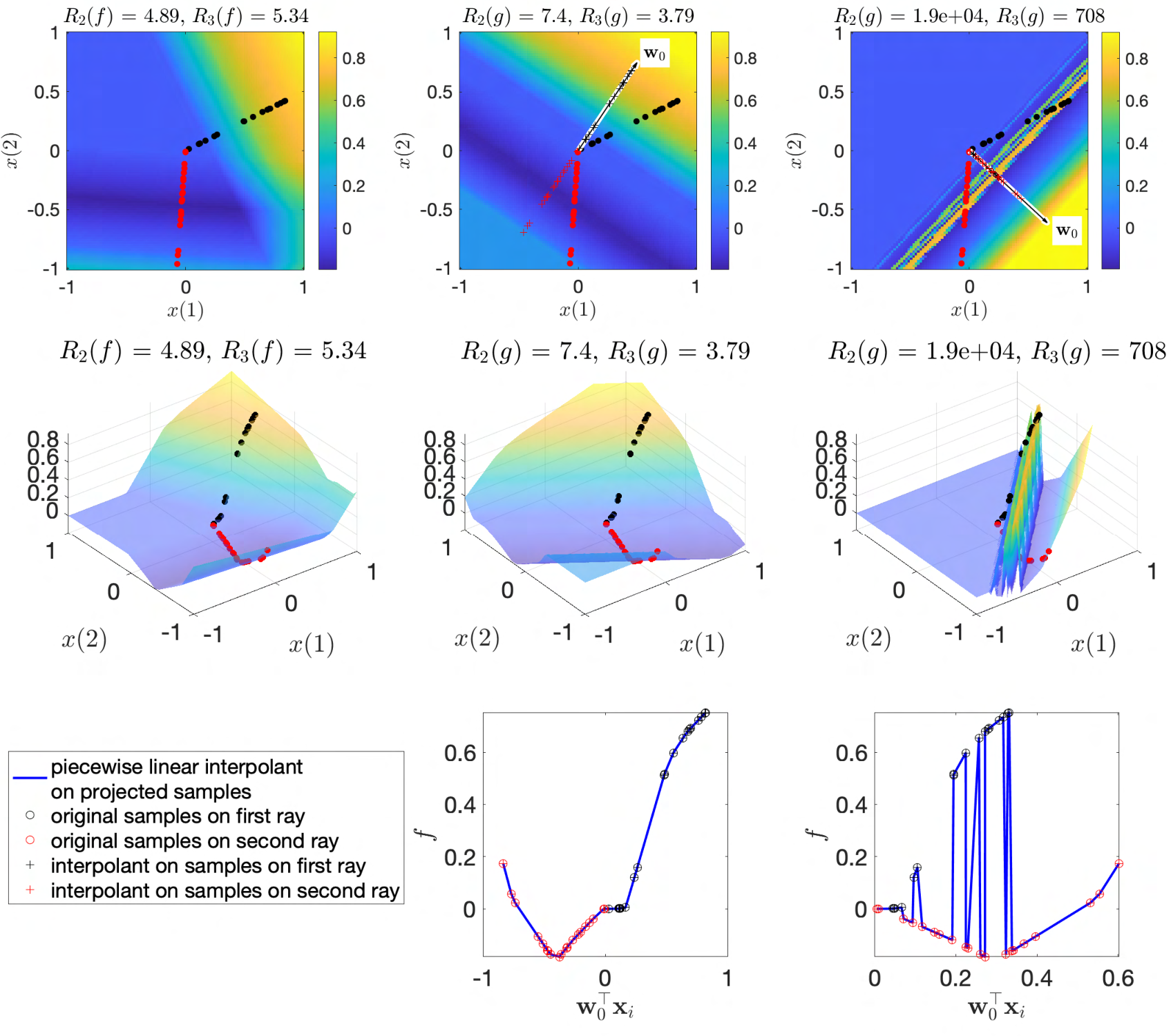
This setting with samples on two rays is illustrated in Figure 3 with ${\bm{w}}_{1}=[2,1]^{\top}$ and ${\bm{w}}_{2}$ is ${\bm{w}}_{1}$ rotated $120^{\circ}$ (before normalization). Note that both $f$ and $g$ fit the training samples exactly but have very different behavior away from the subspaces supporting the training data. In the two-layer setting, ReLU units may be unaligned with one another, and instead align with the support of the training samples (in this case ${\bm{w}}_{1}$ and ${\bm{w}}_{2}$) in order to minimize the $R_{2}$-cost, leading to complex behavior away from this support that presents challenges for out-of-distribution generalization analysis.

In contrast, the $R_{3}$-cost induced by adding a linear layer promotes units that are aligned with a subspace ${\cal S}$, such that there exists some $f\in N_{2}(\mathbb{R}^{d})$ with $y_{i}=f({\bm{P}}_{\cal S}{\bm{x}}_{i})\;\forall i$. That is, even if the training samples do not lie on a subspace, if there is a subspace onto which the samples may be projected while still admitting an interpolant, then that interpolant may have a lower $R_{3}$-cost, depending on the angle $\theta$ between ${\bm{w}}_{1}$ and ${\bm{w}}_{2}$, as shown in Figure 4. The resulting alignment of the ReLU units yields less complex behavior of $\hat{f}$ away from the support of the training samples, potentially leading to better out-of-distribution generalization.

Superficially, one might think the $R_{3}$ representation cost in Lemma 3.4 associated with a network with linear layers composed with a two-layer ReLU network is lower when ${\bm{W}}$ has lower rank – i.e. when the ReLU units are more aligned. However, the $R_{3}$ representation cost offers a more nuanced perspective because it highlights the interplay between the ReLU unit alignment with their scale (i.e. ${\bm{a}}$). To see this, first note that for finite training samples, we may project them all into a subspace ${\cal S}$ for which no two distinct points are projected to the same location and then learn an interpolating function using these projected samples as feature vectors. As described in Section 4, the minimum $R_{L}$ interpolant found using this procedure will have all ReLU weight vectors ${\bm{w}}_{k}\in{\cal S}$, so that $\rank({\bm{W}})=\dim({\cal S})$. In other words, it is generally possible to find interpolating functions with aligned ReLU units. However, some ${\cal S}$ will lead to larger $R_{3}$ representation costs than others. As illustrated in Figure 5, a poor choice of ${\cal S}$ (spanned by ${\bm{w}}_{0}$ in the figure) will lead to a configuration of projected samples that can only be interpolated by a piecewise linear function with many pieces (third column), while they may be interpolated with many fewer linear pieces for alternative ${\cal S}$ (first column with ${\cal S}=\mathbb{R}^{2}$ and second column with ${\cal S}=\sspan({\bm{w}}_{0})$). In other words, forcing ReLU units to lie in a poorly-chosen subspace may yield greater ReLU alignment by requiring many more units – i.e., by sacrificing sparsity.

The representation cost in (14) accounts for both the alignment (through ${\bm{W}}$ and the nuclear norm) and the sparsity (through ${\bm{a}}$). From here, we may infer that adding a linear layer to a two-layer ReLU network does more than “promote alignment of ReLU units”: when searching for interpolants of finite training datasets, training a ReLU network with additional linear layers implicitly seeks a low-dimensional subspace such that a parsimonious two-layer ReLU network can interpolate the projections of the training samples onto the subspace. Note that we are not assuming that the training samples lie on a low-dimensional subspace; that is, we would not see the same effect by simply performing PCA on the training features before training the network. Rather, the best choice of subspace here depends heavily on the training labels.

References

- Arora et al., (2018) Arora, S., Cohen, N., and Hazan, E. (2018). On the optimization of deep networks: Implicit acceleration by overparameterization. In International Conference on Machine Learning, pages 244–253. PMLR. http://proceedings.mlr.press/v80/arora18a/arora18a.pdf.
- Arora et al., (2019) Arora, S., Cohen, N., Hu, W., and Luo, Y. (2019). Implicit regularization in deep matrix factorization. Advances in Neural Information Processing Systems, 32:7413–7424.
- Ba and Caruana, (2013) Ba, L. J. and Caruana, R. (2013). Do deep nets really need to be deep? arXiv preprint arXiv:1312.6184.
- Dai et al., (2021) Dai, Z., Karzand, M., and Srebro, N. (2021). Representation costs of linear neural networks: Analysis and design. Advances in Neural Information Processing Systems, 34.
- Daniely, (2017) Daniely, A. (2017). Depth separation for neural networks. In Conference on Learning Theory, pages 690–696. PMLR.
- Golubeva et al., (2020) Golubeva, A., Neyshabur, B., and Gur-Ari, G. (2020). Are wider nets better given the same number of parameters? arXiv preprint arXiv:2010.14495. https://arxiv.org/pdf/2010.14495.pdf.
- Gunasekar et al., (2018) Gunasekar, S., Woodworth, B., Bhojanapalli, S., Neyshabur, B., and Srebro, N. (2018). Implicit regularization in matrix factorization. In 2018 Information Theory and Applications Workshop (ITA), pages 1–10. IEEE.
- Hanin, (2019) Hanin, B. (2019). Universal function approximation by deep neural nets with bounded width and relu activations. Mathematics, 7(10):992.
- Hanson and Pratt, (1988) Hanson, S. and Pratt, L. (1988). Comparing biases for minimal network construction with back-propagation. Advances in neural information processing systems, 1:177–185.
- Loshchilov and Hutter, (2017) Loshchilov, I. and Hutter, F. (2017). Decoupled weight decay regularization. arXiv preprint arXiv:1711.05101.
- Mulayoff et al., (2021) Mulayoff, R., Michaeli, T., and Soudry, D. (2021). The implicit bias of minima stability: A view from function space. Advances in Neural Information Processing Systems, 34.
- Neyshabur et al., (2017) Neyshabur, B., Bhojanapalli, S., Mcallester, D., and Srebro, N. (2017). Exploring generalization in deep learning. Advances in Neural Information Processing Systems, 30:5947–5956.
- Neyshabur et al., (2015) Neyshabur, B., Tomioka, R., and Srebro, N. (2015). Norm-based capacity control in neural networks. In Conference on Learning Theory, pages 1376–1401. PMLR.
- Ongie et al., (2019) Ongie, G., Willett, R., Soudry, D., and Srebro, N. (2019). A function space view of bounded norm infinite width relu nets: The multivariate case. arXiv preprint arXiv:1910.01635.
- Parhi and Nowak, (2021) Parhi, R. and Nowak, R. D. (2021). Banach space representer theorems for neural networks and ridge splines. J. Mach. Learn. Res., 22(43):1–40.
- Razin and Cohen, (2020) Razin, N. and Cohen, N. (2020). Implicit regularization in deep learning may not be explainable by norms. arXiv preprint arXiv:2005.06398.
- Razin et al., (2021) Razin, N., Maman, A., and Cohen, N. (2021). Implicit regularization in tensor factorization. arXiv preprint arXiv:2102.09972.
- Safran et al., (2019) Safran, I., Eldan, R., and Shamir, O. (2019). Depth separations in neural networks: what is actually being separated? In Conference on Learning Theory, pages 2664–2666. PMLR. http://proceedings.mlr.press/v99/safran19a/safran19a.pdf.
- Savarese et al., (2019) Savarese, P., Evron, I., Soudry, D., and Srebro, N. (2019). How do infinite width bounded norm networks look in function space? In Conference on Learning Theory, pages 2667–2690. PMLR. http://proceedings.mlr.press/v99/savarese19a/savarese19a.pdf.
- Shang et al., (2020) Shang, F., Liu, Y., Shang, F., Liu, H., Kong, L., and Jiao, L. (2020). A unified scalable equivalent formulation for Schatten quasi-norms. Mathematics, 8(8):1325.
- Srebro et al., (2004) Srebro, N., Rennie, J. D., and Jaakkola, T. S. (2004). Maximum-margin matrix factorization. In NIPS, volume 17, pages 1329–1336. Citeseer.
- Steinberg, (2005) Steinberg, D. (2005). Computation of matrix norms with applications to robust optimization. Research thesis, Technion-Israel University of Technology, 2.
- Urban et al., (2016) Urban, G., Geras, K. J., Kahou, S. E., Aslan, O., Wang, S., Caruana, R., Mohamed, A., Philipose, M., and Richardson, M. (2016). Do deep convolutional nets really need to be deep and convolutional? arXiv preprint arXiv:1603.05691.
- Vardi and Shamir, (2020) Vardi, G. and Shamir, O. (2020). Neural networks with small weights and depth-separation barriers. arXiv preprint arXiv:2006.00625.
- Yuan and Lin, (2006) Yuan, M. and Lin, Y. (2006). Model selection and estimation in regression with grouped variables. Journal of the Royal Statistical Society: Series B (Statistical Methodology), 68(1):49–67.
Appendix A Proofs of Results in Section 3
A.1 Proof of Theorem 3.1
While Theorem 3.1 can be proved by more direct means, we use the machinery developed in Section 3 to give a quick proof: In the univariate setting, the product of all linear-layers reduces to a column vector , which is necessarily a rank-one matrix. Therefore, Theorem 3.1 is a a direct consequence of Corollary 3.6, which is a special case of Proposition 3.5, proved below.
A.2 Proof of Lemma 3.2
The result is a direct consequence of the following variational characterization of the Schatten- quasi-norm for where is a positive integer:
where the minimization is over all matrices of compatible dimensions. The case is well-known (see, e.g., Srebro et al., 2004). The general case for is established in (Shang et al., 2020, Corollary 3).
A.3 Proof of Lemma 3.4
For any fixed , we may separately minimize over all scalar multiples where , to get
The last step follows by the weighted AM-GM inequality: , which holds with equality when . Here we have and , and there exists a for which , hence we obtain the lower bound.
Finally, performing the invertible change of variables , we have , and so