Pipeflow: An Efficient Task-Parallel Pipeline Programming Framework using Modern C++Conference: ACM Symposium on High-Performance Parallel and Distributed Computing; June 27–July 1, 2022; Minneapolis, Minnesota, USA

Pipeline parallelism is commonly used to parallelize various applications, such as stream processing, video processing, and dataflow systems. These applications exhibit parallelism in the form of a linear pipeline, where a linear sequence of abstraction functions, namely stages, $F=\langle f_{1},f_{2},\cdots,f_{j}\rangle$, is applied to an input sequence of data tokens, $D=\langle d_{1},d_{2},\cdots,d_{i}\rangle$. A linear pipeline can be thought of a loop over the data tokens of $D$. Each iteration $i$ processes an input token $d_{i}$ by applying the stage functions $F$ to $d_{i}$ in order. Depending on the number of parallel lines, $L=\langle l_{1},l_{2},\cdots,l_{k}\rangle$, to process data tokens, parallelism arises when iterations overlap in time. For instance, the execution of token $d_{i}$ at stage $f_{j}$ of line $l_{k}$, denoted as $f^{k}_{j}$($d_{i}$), can overlap with $f^{k+1}_{j-1}$($d_{i+1}$). A stage can be a parallel type or a serial type to specify whether $f^{k}_{j}$($d_{i}$) can overlap with $f^{k+1}_{j}$($d_{i+1}$) or not. Figure 1 shows the dependency diagram of a 3-stage (serial-parallel-serial) pipeline.

Mainstream pipeline programming libraries employ data-centric models. Users declare input and output data types for each stage using library-specific data abstractions (e.g., template instantiation). Taking oneTBB (TBB eTBB) for example, Listing 1 implements Figure 1 using four parallel lines and a series of callable objects called filter, where each filter receives an input data, performs work on that data, and then produces a result for the next filter. To support arbitrary application data types, libraries typically leverage dynamic polymorphism to allocate and convert data from a generic type (e.g., void*, std::any) to an application type. To further minimize the allocation cost, some libraries, such as oneTBB (TBB eTBB), have implemented specialized object allocators and buffer structures to handle temporary results between stages.

Pipeflow is motivated by our research projects on developing parallel timing analysis algorithms for very large scale integration (VLSI) computer-aided design (CAD). Timing analysis is a critical step in the overall CAD flow because it validates the timing performance of a digital circuit. As design complexity continues to grow exponentially, the need to efficiently analyze the timing of large designs has become the major bottleneck to the design closure flow. For instance, generating a comprehensive timing report (e.g., pessimism removal, hundreds of corners, etc.) for a multi-million-gate design can take several hours to finish (Kahng 2018). To reduce the long analysis runtime, recent years have seen increasing adoptions of manycore parallelism by new timing analysis algorithms (Ajayi et al. 2019).

The most widely used strategy, including commercial timers, to parallelize timing analysis is pipeline. Figure 2 illustrates this strategy using forward timing propagation as an example (Huang et al. 2021). The circuit graph is first levelized into a level list using topological sort. Nodes at the same level are independent of each other and can run in parallel. Each node runs a sequence of linearly dependent propagation tasks, including parasitics (RCP), slew (SLP), delay (DLP), arrival time (ATP), jump points (JMP), and common path pessimism reduction (CRP) to update its timing data from a custom circuit graph data structure. Different propagation tasks can overlap across different levels using pipeline parallelism.

In fact, this type of task-parallel pipeline strategy is ubiquitous in many parallel CAD algorithms, such as logic simulation and physical design, because computations frequently depend on circuit networks. We have observed three important properties that make mainstream pipeline programming frameworks fall short of our need: 1) Unlike the typical data-parallel pipeline, the pipeline parallelism in many CAD algorithms is driven by tasks rather than data. 2) Data is not directly involved in the pipeline but the graph data structure crafted by a custom algorithm. 3) From user’s standpoint, the real need is a pipeline scheduling framework to help schedule and run tasks on input tokens across parallel lines, while leaving data management completely to applications; in our experience, users disfavor another library data abstraction to perform pipeline scheduling, as it often incurs development inconvenience and unnecessary data conversion overheads.

Taskflow is a general-purpose parallel and heterogeneous programming system using modern C++ (Huang et al. 2022). Taskflow introduces a new control taskflow graph (CTFG) model that enables end-to-end implementation of task graph parallelism coupled with in-graph control flow. A CTFG consists of several task types, such as static task, dynamic task, condition task, module task, runtime task, and so on. Figure 3 shows a CTFG of iterative tasking, implemented in Listing 2. The loop continuation condition is implemented by a single condition task, cond, that precedes two static tasks, body and done. When cond returns 0, the execution loops back to body. When cond returns 1, the execution moves onto done and stops. This example uses four tasks to implement a tasking loop of 100 iterations.

Another powerful feature of Taskflow is composable tasking. Composable tasking enables users to define task hierarchies and compose large task graphs from modular and reusable algorithm blocks that are easier to optimize. Figure 4 gives an example of a Taskflow graph using composition. The top-level taskflow defines one static task C that runs before a dynamic task D that spawns two dependent tasks D1 and D2. Task D precedes a module task E composed of a taskflow of two dependent tasks A and B. Listing 3 shows the Taskflow code of Figure 4. It declares two taskflows, taskflow1 and taskflow2. The second taskflow defines a module task that is composed of the first taskflow, preceded by task D. A module task does not own the taskflow but maintains a soft mapping to the taskflow. Users can create multiple module tasks from the same taskflow, but they must not run concurrently.

Pipeflow leverages modern C++ and template techniques to strike a balance between expressiveness and generality. Listing 4 shows the Pipeflow counterpart of the oneTBB code in Listing 1 that implements the pipeline in Figure 1. There are three steps to create a Pipeflow application, 1) define the pipeline structure using template instantiation, 2) define the data storage, if needed, and 3) define the pipeline task using taskflow composition. Users define the number of parallel lines and the abstract function of each stage in a tf::Pipeline object. For each stage, users define the stage type and a pipe callable using tf::Pipe. A stage can be either a serial type (tf::PipeType::SERIAL) or a parallel type (tf::PipeType::PARALLEL). The pipe callable takes an argument of tf::Pipeflow type which is created by the scheduler at runtime. A tf::Pipeflow object represents a scheduling token and contains several extensible methods for users to query the runtime statistics of that token, including the line, pipe, and token numbers. In Pipeflow, pipe and stage are interchangeable.

Pipeflow does not have any data abstraction but gives applications full control over data management. In our example, since the first and the second pipes generate float and std::string outputs, respectively, we create a one-dimensional (1D) array, buf, to store data in a uniform storage using std::variant<float, std::string>. The dimension of the array is equal to the number of parallel lines, as Pipeflow schedules only one token per line. Each entry buf[i] stores the data that is being processed at line $i$, which can be retrieved by tf::Pipeflow::line. This organization is very space-efficient because we use only 1D array to represent data processing in a two-dimensional (2D) scheduling map. Additionally, by delegating data management to applications, we can avoid dynamic data conversion between the library and the application, which typically counts on virtual function calls to convert a generic type (e.g., void*, std::any) to an arbitrary user type (TBB eTBB; Aldinucci et al. 2017).

Based on the above pipeline structure and data layout, we instantiate a tf::Pipeline object, pl. This template-based design enables the compiler to optimize each pipe type, such as using fixed-layout functor to store the callable and its captured data. Finally, we create a pipeline module task pipeline with pl using the taskflow composition method composed_of and submit this taskflow to an executor to run the pipeline.

tf::Pipeline requires instantiation of all pipes at the construction time. While this design gives compilers freedom to optimize the layout of each pipe type, it prevents applications from varying the pipeline structure at runtime; for instance, the number of pipes might depend on the problem size, which can be runtime variables. To overcome this limitation, Pipeflow provides a scalable alternative, tf::ScalablePipeline, to allow variable assignments of pipes using range iterators. In Listing 5, we create a scalable pipeline, pl, from a vector of six pipes. After the first run, we reset pl to another range of three pipes for the next run. A scalable pipeline is thus more flexible for applications to create pipeline scheduling framework with dynamic structures.

A key advantage of Pipeflow is its composability with Taskflow. By encapsulating a pipeline in a module task, we enable seamless integration with all existing task types in Taskflow. This result largely facilitates the implementation of complex pipeline applications that require intensive interaction with different types of task parallelism. Figure 5 shows a Taskflow graph that emulates a data streaming application using a pipeline module task and a condition task. The condition task is used to decide if the pipeline needs to be run again depending on the application control flow. Listing 6 shows the Taskflow code of Figure 5, using the pipeline task in Listing 4. When the condition task cond returns 0, it informs the scheduler to rerun the pipeline task pl, or proceeds to done to stop the program otherwise.

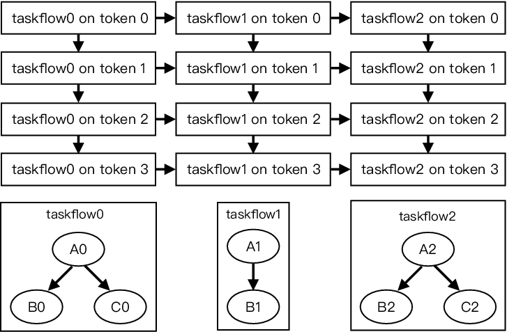
Figure 6 demonstrates another common application that embeds task graph parallelism inside a pipeline. The pipeline consists of three serial stages and four parallel lines. Each scheduled token runs a taskflow that implements a stage algorithm in the pipeline. The three taskflows are self-explanatory. Different taskflows can overlap across different lines, but only one taskflow runs on the same stage due to the serial type. Listing 7 implements Figure 6. We create a 1D array, buf, to store the three taskflows (defined elsewhere). In each stage, we obtain its taskflow at buf[pf.pipe()], submit it to the executor, and wait until the execution finishes. As we need only four tokens, the first pipe stops the scheduler at the fifth.

Pipeflow leverages Taskflow’s work-stealing runtime to design an efficient scheduling algorithm with dynamic load balancing. As Pipeflow does not touch data abstraction, we can simplify the pipeline scheduling problem to deciding which task to run at which pipe and line. Similar to oneTBB, the key idea of our scheduling algorithm is to enable only one scheduling token per line and process all tokens in a circular fashion across all parallel lines. Based on the idea, we formulate the pipeline scheduling into a lightweight Taskflow graph where 1) one task deals with a scheduling token per line and 2) each task decides which task to run on its next line and pipe using simple atomic operations.

Pipeflow creates a taskflow for each pipeline module task using one condition task and multiple runtime tasks one per line. A runtime task is a task type in Taskflow for users to interact with the executor (Huang et al. 2022), such as scheduling a task in the graph. The condition task decides which runtime task to run when the pipeline starts. A runtime task deals with a scheduling token at a line and will create a pipeflow object (of type tf::Pipeflow) to pass to the pipe callable. Figure 7 shows the taskflow of the pipeline module task in Listing 7. As there are four parallel lines, the task graph consists of one condition task, cond, and four runtime tasks, rt-0, rt-1, rt-2, and rt-3. Ultimately, only five tasks are used to run the pipeline, even though the execution can involve many scheduling tokens.

Algorithm 1 implements the construction of the Taskflow graph for a pipeline. First, we define the condition task to return on the index of the next task (line 1). Since the pipeline is running in a circular fashion, the index is equal to the remainder of the total number of scheduled tokens divided by the number of parallel lines. Next, we define the runtime task using build_runtime_task for each line (line 1) and specify the dependency between each runtime task and the condition task (line 1).

Algorithm 2 implements build_runtime_task. When a runtime task is scheduled, we need to know which stage at which line for the scheduling token to work. We keep the line and stage information in a Pipeflow object. Each runtime task owns a Pipeflow object pf of a specific line (line 2). Once a scheduling token is done, there are two cases for its runtime task to proceed: 1) for a parallel type, the runtime task moves to the next stage at the same line; 2) for a serial type, the runtime task additionally checks if it can move to the next line. To carry out such a dependency constraint, each stage keeps a join counter of an atomic integer to represent its dependency value. The values of a serial stage and a parallel stage can be up to 2 and 1, respectively. We create a 2D array jcs to store the join counter of each stage at each line. Line 2 initializes these join counters to either 2 or 1 based on the corresponding stage types that are enumerated on integer constants, 2 (serial) and 1 (parallel). At the first stage (line 2), the Pipeflow object updates its token number (line 2) and checks if the pipe callable requests to stop the pipeline (lines 2:2). If continued, we increment the number of scheduled tokens by one (line 2). For other stages, we simply invoke the pipe callables (lines 2:2).

After the pipe callable returns, we update the join counters based on the stage type and determine the next possible tasks to run (lines 2:2). When the join counter of a stage becomes 0, we bookmark this stage as a task to run next (line 2 and line 2). If two tasks exist (line 2), the current runtime task informs the scheduler to call a worker thread from the executor to run the task at the next line (line 2) and reiterates itself on the next pipe (line 2). The idea here is to facilitate data locality as applications tend to deal with the next stage as soon as possible. If there is only one task available, the current runtime task directly runs the next task with the updated pf object (lines 2:2).

Figure 8 illustrates our scheduling algorithm using the pipeline in Listing 7. Since the pipeline runs in a circular fashion, there are four dependencies (dashed edges) from the last stages to the first stages, and one dashed edge from the first stage of the last line to the first stage of the first line. Each line runs only one scheduling token. Multiple lines overlap tokens in a circular fashion. Compared to existing algorithms, such as oneTBB (TBB eTBB), that count on non-trivial synchronization between tasks and internal data buffers, our algorithm focuses on the task parallelism itself and thus largely reduces the scheduling complexity of pipeline using simple atomic operations. We draw the following lemmas and sketch their proofs to justify the correctness of our scheduling algorithm:

Given a large number of pipeline programming frameworks, it is infeasible to compare Pipeflow with all of them. Each of them has its pros and cons and dominates certain applications. Since Pipeflow is inspired by our CAD applications, we select oneTBB Parallel Pipeline (v2021.5.0) (TBB eTBB) as our baseline, which has been widely used in the CAD community. We believe this selection is sufficient and fair to highlight the advantage of Pipeflow, considering the similar tasking infrastructure between oneTBB and Pipeflow. For oneTBB pipelines, we pass a nominal integer between successive stages (i.e., tbb::filter), because oneTBB does not allow void type but implements a specialized memory allocator to hold intermediate results returned by stages.

The purpose of micro-benchmarks is to measure the pure scheduling performance of Pipeflow without much computation bias from the application. We compare the runtime and memory between Pipeflow and oneTBB for completing pipelines of different numbers of serial stages, scheduling tokens, and threads. We do not use parallel stages as the callable of a parallel pipe can be absorbed into the previous serial pipe. Each stage performs a nominal work of constant space and time complexity and forwards the scheduling token to the next stage.

Figure 9 draws the runtime improvement of Pipeflow over oneTBB and memory data under different numbers of scheduling tokens. Here, we use 16 threads, which produce the best performance for both, to run a pipeline of 80 serial stages and 80 parallel lines. With more token numbers ($>$256), Pipeflow is consistently better than oneTBB, despite the slight improvement ($<$1%). When the number of scheduling tokens is small, the variation is large (e.g., up to 6% improvement at 32 tokens). This is because when oneTBB starts the pipeline, it requires expensive set-up time on the data buffers, whereas Pipeflow can immediately start the task scheduling. Yet, as we increase the number of tokens, such cost can be amortized. In terms of memory, oneTBB is always higher than Pipeflow (e.g., 21% at 65K tokens) since we do not manage any data buffers but focus on the task scheduling itself.

Figure 10 draws the runtime and memory performance using 16 threads to schedule 65K tokens through different numbers of stages, where the number of parallel lines is equal to the stage count. We observe that Pipeflow is consistently faster than oneTBB when the number of stages is larger than 16, despite the difference being slight ($<$1%). At 8 stages, the available task parallelism is smaller than the given thread parallelism, and oneTBB is faster in this scenario. This is due to Taskflow’s scheduling algorithm. Taskflow always keeps one thread busy in stealing while there is an active worker. When the available task parallelism is scarce, the scheduling cost becomes expensive. Yet, this problem can be mitigated by users selecting the right line number in their pipeline applications. For instance, beyond 8 stages, Pipeflow starts to outperform oneTBB. In terms of memory, we can clearly see the difference between Pipeflow and oneTBB (e.g., 19% at 80 stages). As we increase the number of stages, oneTBB needs more space for internal data buffers, whereas Pipeflow delegates the data management completely to applications.

Figure 11 shows the runtime and memory results at different numbers of threads to run 65K tokens on a pipeline of 80 stages and 80 parallel lines. Both Pipeflow and oneTBB scale equally well as the number of cores increases. At each point, we observe a small win of Pipeflow. For instance, at 32 cores, Pipeflow is 4.3% faster than oneTBB. In terms of memory, both Pipeflow and oneTBB use more memory with more threads. However, there remains a clear gap between Pipeflow and oneTBB (e.g., 22% less by Pipeflow at 40 cores).

Figure 12 compares the throughput by corunning the same program up to 10 times. We use the weighted speedup to measure the system throughput, which is the sum of the individual speedup of each process over a baseline execution time (Ding et al. 2012). A throughput of one implies that the corun throughput is the same as if those processes run consecutively. On the left, the pipeline has 8 stages and 8 parallel lines. On the right, the pipeline has 80 stages and 80 parallel lines. Both of them run 65K scheduling tokens using 40 threads. The experiment emulates a server-like environment where different pipeline applications compete for the same resources. We can see that Pipeflow outperforms oneTBB in most coruns. For example, at 10 coruns, Pipeflow is 1.1 $\times$ and 1.5$\times$ better than oneTBB with 8 and 80 stages, respectively.

We applied Pipeflow to solve a VLSI static timing analysis (STA) problem. The goal is to analyze the timing landscape of a circuit design and report critical paths that do not meet the given constraints (e.g., setup and hold). As presented in Figure 2, modern STA engines leverage pipeline parallelism to speed up the timing propagations. However, nearly all of them count on OpenMP-based loop parallelism with layer-by-layer synchronization (Huang et al. 2021). With Pipeflow, we can directly formulate the problem as a task-parallel pipeline to improve task asynchrony. As the analysis complexity continues to increase, more analysis tasks (e.g., RC, delay calculators, pessimism reduction) are incorporated into each node in the STA graph. These tasks can be encapsulated in a sequence of stage functions to overlap in graph across parallel lines. We modify a large circuit design of 1.5M nodes and 3.5M edges from (Huang et al. 2021) and study the performance under different stage counts. Each node has a stage task to calculate delay values at a specific configuration using 2D matrix multiplication.

Figure 13 compares the runtime and memory between Pipeflow and oneTBB up to 80 stages. We use 80 parallel lines for all experiments; we do not observe much difference in other numbers of parallel lines as both Taskflow and oneTBB have an adaptive work-stealing strategy to balance the number of running threads with dynamic task parallelism. In general, Pipeflow outperforms oneTBB at large stage numbers. For example, using 40 cores and 72 stages, Pipeflow is 10% faster than oneTBB. In terms of memory usage, Pipeflow is always better than oneTBB regardless of the number of stages and cores. Pipeflow consumes less memory than oneTBB does because all stage tasks perform computations directly on a global graph data structure captured in the pipe callable. The data passing interface between successive stages in oneTBB thus becomes a significant yet unnecessary overhead.

Next, we compare the throughput by corunning the same program up to 10 times. Corunning an STA program is very common for reporting the timing data of a design at different input library files (Kahng 2018). The effect of pipeline scheduling propagates to all simultaneous processes. Hence, throughput is a good measurement for the inter-operability of a pipeline-based STA algorithm. We corun the same analysis program up to 10 processes that compete for 40 cores. Again, we use the weighted speedup to measure the throughput. Figure 14 plots the throughput across 10 coruns at 8 and 80 stages. We can see that Pipeflow outperforms oneTBB at all coruns. For instance, at 10 coruns, Pipeflow is 1.7$\times$ and 1.2 $\times$ better than oneTBB with 8 and 80 stages, respectively.

We applied Pipeflow to solve a VLSI detailed placement problem. Detailed placement is a critical step in physical optimization. The goal is to optimize the interconnect among millions of logic gates or instances for improved timing and power. Connected instances are grouped to a net with interconnect modeled in Manhattan distance. We consider the detailed placement algorithm in DREAMPlace (Lin et al. 2020), namely local reordering. The algorithm decides an optimal order of four consecutive instances in a window of a placement row that produces minimum interconnect wirelength. We can parallelize the reordering algorithm using pipeline. Each row corresponds to a parallel stage that finds the best ordering of cells in a window from the top to the bottom. The scheduling tokens sweep through all windows from the left to the right. Figure 15 illustrates the algorithm.

Figure 16 compares the runtime and memory data between Pipeflow and oneTBB for two industrial designs, adaptec1 and bigblue4. adaptec1 is a medium design with 211K instances and 221K nets (instance dependencies), defining 890 stages for 890 placement rows and 10692 windows. bigblue4 is a large design with 2.1M instances and 2.2M nets, defining 2694 stages for 2694 placement rows and 32190 columns. Both Pipeflow and oneTBB scale with increasing numbers of cores, whereas Pipeflow always outperforms oneTBB 3–24%. For instance, in bigblue4 (40 cores), Pipeflow finishes the placement algorithm in 6131 seconds, whereas oneTBB needs 8213 seconds. Such improvement is significant as practical design closure process can invoke millions of placement iterations to optimize the physical layout. Likewise, Pipeflow outperforms oneTBB in memory usage. The difference is slight (about 1%) because most memory is taken by the placement problem itself, including the data structure of rows and instances.

As an experienced parallel CAD researcher, Pipeflow has assisted us to overcome many programming challenges. In the previous two experiments, the data is explicitly managed by the application algorithms and does not go through any data abstraction layers of oneTBB. The real need is a task-parallel pipeline programming framework that 1) gives us full control over data and 2) allows us to probe each scheduled task. For instance, when implementing the placement algorithm, we capture the row data from a global database in each pipe callable and use the pipeflow variable to get the line numbers of a scheduled task to index its window locations. However, oneTBB has abstracted these components out, and we have to implement another mapping strategy to get these data from each filter. Similar problems exist in other libraries too.