Complete evaporation of black holes and
Page curves
Abstract
The problem of complete evaporation of Schwarzschild black holes raised by Hawking is that one has an explosion of the temperature for vanishing black hole mass . We consider the Reissner-Nordstrom black hole and note that if mass and charge satisfy the bound , for small then the complete evaporation of black holes without blow-up of temperature is possible. We describe curves on the surface of state equations such that the motion along them provides complete evaporation. The radiation entropy follows the Page curve and vanishes at the end of evaporation. Similar results for rotating Kerr, Schwarzschild-de-Sitter and Reissner-Nordstrom-(Anti)-de-Sitter black holes are discussed.
1 Introduction
It was suggested by Hawking that the Schwarzschild black holes produce radiation like black bodies with temperature
of , where is the mass of the black hole Haw1.
During this process, the mass of the black hole is lowered and the temperature is increased. It is an open question whether this process continues until the entire mass of the black hole has been converted to radiation or whether it stops when the mass is close to the Planck mass Haw1; Haw2; Page:2013dx; Susskind; FN. In this paper, we study under which conditions in classical gravity the complete evaporation of black holes is possible.
According to the Stefan-Boltzmann law, the energy density of black body radiation with temperature is given by
Therefore from Hawking’s formula for the temperature, it follows that the energy density of the radiation, emitted by a black hole behaves at small as .
If the mass of the black hole disappears during evaporation, then the black hole releases an infinite amount of energy, which is clearly unphysical. Hawking drew attention to this problem in his first paper on the evaporation of black holes with the title ”Black hole explosions?” Hawk3.
The information loss problem Haw2; Page:1993wv is closely related to this unphysical behaviour, since the radiation entropy diverges for small as .
One can say that because of this infinity, complete evaporation never occurs in nature, and we cannot obtain complete evaporation, which ends only by thermal radiation being obviously a mixed state.
Just the evolution of the initially pure quantum state to this mixed state breaks unitarity and leads to information paradox.
In this paper, a possible mechanism for the complete evaporation without temperature explosion of black holes in the framework of classical gravity is discussed. This mechanism also ensures that the entropy of radiation vanishes in the limit when the mass of the black hole tends to zero, which is consistent with unitary evolution.
We note that the complete evaporation without explosion of temperature and energy is possible if the black hole possess addition parameters – a charge or an angular momentum , or we deal with non-zero cosmological constant and we are in near-extremal regimes.
In the case of the Reissner-Nordstrom black hole if the mass and charge satisfy also the bound
| (1.1) |
for small mass , then the Hawking temperature for the charged black hole
| (1.2) |
tends to 0 when .
We can describe special curves in the domain (1.1). The expression (1.2) defines the surface of the state equation in the 3-dimensional space with coordinates . Evaporation process is described by a curve on : , , , where is a time variable (see Fig.1.A in Sect.2). It is convenient to make the change of variables , . We describe an evaporation curve by a function and the charge belong this curve is
| (1.3) |
where . Obviously, the Reissner-Nordstrom solution of the Einstein equations with parameters and will still be a solution if the charge is taken to depend on the mass . The Hawking temperature becomes
| (1.4) |
If we take such that for small it obeys
,
then tends to as and we get the complete evaporation of the black hole. Therefore, for small , the evaporating black hole must be in a state close to the extreme one.
In this paper we consider two particular examples of near extremal Reissner-Nordstrom black holes.
- •
We take
(1.5) This means that for small we are dealing with almost extreme regime. An interesting case is when , i.e. . In this case, the limit of temperature when is not equal to zero, but is equal to , although the mass and charge are vanishing. In the cases with the mass dependence of charge has a deformed bell-shaped form (see Fig.2.A below).
- •
We also consider the case then the function is given. In this case one can solve the quadratic equation (1.4) and find the function . We take as an example the temperature of the form
(1.6) where and are positive constants and . The radiation entropy is proportional to so in this case one has .
As mentioned above, the problem of temperature explosion during evaporation of the black hole is closely related with the information paradox. In the context of studying the information paradox, Page Page:1993wv; Page:2013dx
proposed that the Schwarzschild black holes evaporate completely and the radiation entropy of evaporating
black holes first increases but then decreases and tends to zero when the black hole mass vanishes. This hypothetical behavior is known as the Page curve. Recent works devoted to the information paradox are aimed to obtain the Page curve
Penington:2019npb; Almheiri:2019psf; Almheiri:2019hni for the entanglement entropy of radiation. In this work we deal with the usual thermodynamic entropy for radiation that is proportional to . So if temperature decreases with vanishing of mass then the entropy of radiation decreases too. To get the time dependence of this evolution we consider charge and mass change during the black hole evaporation.
The loss of the mass and charge during evaporation of the Reissner-Nordstrom black hole is a subject of numerous considerations. Changes in mass and charge during the evaporation of a RN black hole satisfy a system of two coupled equations (see below eqs. (2.28) and (2.29)). Assuming that the relation between mass and charge is fixed, we are left with a single non-linear differential equation
| (1.7) |
where an explicit expression for the function is given in Sect.2.3. For small and we get mass evolution in the form
| (1.8) |
where and are positive constants. This form of time dependence of mass of evaporation black hole together with radiation entropy dependence as provide the Page form of time evolution of the radiation entropy, Fig.5.A - Fig.5.C. If then In this case the leaving time of black hole is infinite and the the evolution of the radiation has the form presented in Fig.5.C
and Fig.5.E.
For Kerr, Schwarzschild de Sitter
and Reissner-Nordström-(Anti)-de Sitter black holes, we also indicate the curves on the equation of the state surfaces along which the complete evaporation of black holes occurs without thermal explosions.
The paper is organized as follows. In Sect.2 models of complete evaporation of the Reissner-Nordstrom black hole accompanied by the temperature goes to are considered. In Sect.3 the models of complete evaporation of the Kerr black hole are investigated and in Sect.4 these results are generalized to the Kerr-Newman black hole. Complete evaporation of the Schwarzschild-de-Sitter black hole is considered in Sect.5. In Sect.6 we discuss complete evaporation of Reissner-Nordstrom-(Anti)-de-Sitter black holes. Sect.7 contains summary and discussions.
2 Complete evaporation of the Reissner-Nordstrom black hole
We consider a model of complete evaporation of a Reissner-Nordstrom (RN) black hole with the following metric
| (2.9) |
where
| (2.10) |
here and are mass and charge of the black hole. It is assumed that . The blackening function (2.10) can be presented as
| (2.11) |
where
| (2.12) |
The temperature of the Reissner-Nordstrom black hole is
| (2.13) |
2.1 Evaporation curves and bell-shaped temperature
We take to be a function on of the form (1.3). The Hawking temperature under this constraint becomes equal to
| (2.14) |
Depending on the behavior of the function we have:
- •
if satisfies for small the bounds
(2.15) then as and one gets the complete evaporation of black hole;
- •
if the function satisfies the bounds
(2.16) then the temperature also for ;
- •
if the function is
(2.17) then the temperature and also for . Note that the asymptotic of at coincides with the Schwarzschild case.
The entropy and the free energy under constraint (1.3) are equal
| (2.18) | |||||
| (2.19) |
Note that the entropy and the free energy go to as for
satisfying (2.15).
Let us suppose that the temperature is given by a function . We solve the quadratic equation (2.14) and find two functions
| (2.20) |
Both solutions are real for
| (2.21) |
2.2 Examples
2.2.1 Deformed bell-shaped dependence of charge on mass
Equation (2.13) defines the surface of the state equation for Reissner-Nordstrom black hole. This surface is shown in Fig.1.A. The same surface is shown in Fig.1.B in coordinates, eq. (2.14).

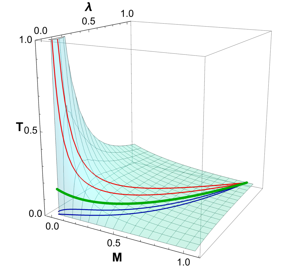
A B
The 3D curves in Fig.1.A and Fig.1.B show the dependence of temperature on mass along the curves
| (2.22) |
with different . We see that on some curves the temperature tends to infinity as (for these curves ), while on curves with the temperature tends to zero as .
A B
Mass dependence of charge , temperature , entropy and free energy at (2.22) with different parameters and the same parameter are shown in fig.2. We see that for all there is a restriction on , . The temperature and entropy of the radiation tend to zero at for , to a nonzero constant for , and to infinity for . In this case, the temperature and radiation entropy at , starting from the initial value at , increase to a certain maximum value, then decrease to zero, i.e. the mass dependencies and have deformed bell shapes (the thickest red and dark cyan lines in Fig.2.A and B, respectively). In the case of a slow dependence of mass on time during black hole evaporation, the dependence of radiation entropy on mass, represented in Fig.2.B by the dark cyan line, leads to the Page form of the time evolution of radiation entropy, see Fig.5. The entropy of a black hole and the free energy tend to zero at for all values of . We also see, Fig.2.A, that the shape of Q versus is a deformed bell (except in the case of and , which corresponds to the Schwarzschild case). Note that in fig.2.B one can see that the free energy increases as the black hole mass decreases. This corresponds to the region , where the charge increases with decreasing mass .
In our recent paper Arefeva:2022cam we found restrictions on in (2.22) under which the entanglement entropy calculated with the island formula has no explosion at .
2.2.2 Semi-circle dependence of temperature on mass
One can take the semi-circle form of dependence on (1.6) with . The condition (2.21) gives a restriction on possible values on admissible . Indeed, substituting (1.6) to the condition (2.21) we get
| (2.23) |
that should be satisfied
for all . This can be realized for .
A B
We plot in Fig.3.A as a function of for two branches given by (2.20), where is defined by (1.6). We see that for small both are real. For two solutions are real only on parts of the interval (dashed blue lines in Fig.3.A). For small and we have
| (2.24) | |||||
| (2.25) |
and in accordance with (2.21) we consider only the -branch.
A
B
We have the following asymptotic behaviour of , , and for small
| (2.26) | |||||
| (2.27) |
The plot in Fig.4.A shows the dependences of the temperature and the entropy of radiation on for two different , and . As has been noted above, there is no a real solution for . The plot in Fig.4.B shows dependences of the entropy (blue) and free energy (green) of the Reissner-Nordstrom black hole on calculated on the branch for different . The vertical black lines indicate the value of , . It is interesting to note that both entropies, the black hole entropy and the radiation entropy have the form suitable to realize the Page curves - they first increase from some initial values, in particular from zero values for the case of the radiation entropy, up to some maximal value, then start to decrease to zero at
2.3 Time evolution
The loss of the mass and charge during evaporation of RN black hole
is a subject of numerous consideration Gibbons-1875; Zaumen; Carter; Damour; Page-1976; Hiscock-1990; Gabriel-2000; Sorkin:2001hf; Ong:2019vnv and refs therein.
In the case of fixed relations (1.3), we consider the following system of equations
| (2.28) | |||||
| (2.29) |
where is a positive constant and the cross-section is proportional to for small . The first equation in the system of equations (2.28) and (2.29) coincides with the equation considered in Hiscock-1990, and the second is obtained by simply differentiating the relation (1.3). From (2.28) and (2.29) we get
| (2.30) |
For and small one gets
| (2.31) |
This equation for and has a solution
| (2.32) |
where and are positive constants. For we have
| (2.33) |
One gets an infinite large time of the complete evaporation of charged black hole under constraint
(1.3).
In Fig.5 we present two different regimes of mass versus time, Fig.5.A and Fig.5.D, the former with a finite decay time and the latter with an infinite decay time. Because of the dependence of radiation entropy on mass shown in fig.5.B, these two different types of time dependence on mass result in two different entropy versus time dependences, Fig.5.C and Fig.5.E. But these two graphs do not differ significantly if we consider them on the interval , here . In both cases, entropy first increases with time, then decreases after Page time . Note that if , we can ignore the effects of quantum gravity in the above consideration.
A B C
D E
3 Complete evaporation of the Kerr black hole
The Kerr metric in Boyer-Linquist coordinates reads
| (3.34) |
where
| (3.35) |
The outer and inner horizon are located at respectively and
| (3.36) |
The temperature of the Kerr black hole is
| (3.37) |
When equal to one gets an extremal black hole with .
If the angular momentum also satisfies the bound
| (3.38) |
for small mass , then the Hawking temperature
tends to 0 when .
If we take to be a function of of the form
| (3.39) |
where the function , then the temperature becomes equal to
| (3.40) |
and the entropy and the free energy are
| (3.41) | |||||
| (3.42) |
If as , then .
Similar to the RN case, if one takes the function as
| (3.43) |
then the temperature and also for .
3.1 Examples
3.1.1 Deformed bell-shaped evaporation curves
As in the previous Sect.2, we first consider the case (2.22). The behaviour of the charge , the temperature , the entropy and the free energy as functions of for the curves
(3.39) with different scaling parameter and the same parameter are presented in Fig.6.
These plots are very similar to the plots presented in Fig.2 for the RN case.
For all there is a restriction on
, and the temperature and the radiation entropy go to zero as for , to a non-zero constant for and to the infinity for . Moreover, the radiation entropy at , starting from the initial value at , first increases to a certain maximum value, then decreases to zero, i.e. has a form that, in the case of a slow decrease in mass during evaporation, provides the form of the Page dependence of the radiation entropy on time, see Fig.5. The black hole entropy (blue lines, Fig.2.B) and the free energy (green lines, Fig.2.B) go to zero when
for . We also see, Fig.6.A, that
the form of dependence of on is a deformed bell,
compare with Fig.2.A.
A B
3.1.2 Semi-circle dependence of temperature on mass
If the function is given, then from equation (3.40) we get
| (3.44) |
Unlike (2.14), now the equation relating and , i.e. equation (3.40), is linear on which gives us (3.44). Assuming the temperature dependence on is the same as for the RN case, (1.6), we get
| (3.45) |
Note that the explicit forms of in the RN and Kerr cases are different, compare (2.20) with (3.44).
For small from (3.45) follows that and the constraint (3.39) corresponds to positive values of . At the critical value of the following equation
| (3.46) |
has one real solution, , and . For equation (3.46)
has two real solutions, for example, for shown in Fig.7, there are two real solutions ,
. Indeed,
in the plots in Fig.7.A we see that for and for there are two intersections of the gray dashed line represented with the red dotted line. The case of one real root of equation (3.46) is shown by thick blue line in Fig.7.A and thick blue line in Fig.7.B.
The plots in Fig.7.C show mass dependences of the temperature and the entropy of radiation, and the plot in Fig.7.D show mass dependences of the black hole entropy and the free energy on for different .
A B
C D
4 Complete evaporation of the Kerr-Newman black hole
The Kerr-Newman (KN) metric is
| (4.47) | |||||
where . Here the parameters , and are the mass, the angular momentum, and the charge of the black hole, respectively. The electromagnetic potential is
| (4.48) |
There are two horizons and
| (4.49) |
The Hawking temperature of the black hole horizon is given by
| (4.50) |
A B
We can put the constraint
| (4.51) |
where is a function of . Substituting (4.51) into (4.50) we get
| (4.52) |
From the first equality in (4.52) for we get
(3.40) and from the second for we get (3.40).
Assuming that , , from (4.51) we get that . The requirement that for forces us to assume .
Solving equation (4.52) in respect to we get
| (4.53) |
Note, that does not enter to (4.53). This equation (4.53) is analogous to equation (2.20), which does not contain . Equation (2.20) follows from (4.53) for . The equivalent representation is
| (4.54) |
from which we get (3.44) for .
Assuming that
| (4.55) |
and substituting this expression in (4.53), we get
| (4.56) |
have different asymptotic for small
| (4.57) | |||||
| (4.58) |
and we take the second branch . On this branch we find the form of the KN black hole entropy and the free energy
| (4.59) | |||||
| (4.60) |
The dependence of the entropy of radiation of KN black hole on for the constraint corresponding to , is presented in Fig.8.A. The dependence of the KN black hole entropy on for the constraint corresponding to , is presented in Fig.8.B. Here these dependences are shown by gray lines for and blue lines for . In Fig.8.B we show also the free energy as functions of for zero (brown lines for free energy) and (green lines for free energy) for two choices of in eq.(4.55), . To different choices of correspond the lines of different thickness.
5 Complete evaporation of the Schwarzschild-de Sitter
black hole
The line element has the form
| (5.61) |
where
| (5.62) |
is the mass of the black-hole and is the positive cosmological constant. For
| (5.63) |
there are 3 horizons, the black hole horizon
| (5.64) |
the cosmological horizon
| (5.65) |
and the negative non-physical one.
The Hawking temperature of Schwarzschild-de Sitter is
| (5.66) |
where is given by (5.64). We can represent the temperature as
| (5.67) |
We see that for fixed the temperature becomes infinite when .
We note that the nominator is equal to zero at and this value of realizes the bounded value of admissible by inequality (5.63).
By analogy with the cases of RN and Kerr considered in the previous sections, we can consider to be dependent on and parametrize this dependence by a function , i.e.
| (5.68) |
We assume that satisfies the bounds . One can check that if
| (5.69) |
then as .
Indeed, since now the temperature is
| (5.70) |
and assuming (5.69) we get the asymptotic expansion for small as
| (5.71) |
We see that if , , then when .
In Fig.9 we present dependence of the temperature (red lines), the black hole entropy (blue lines), the free energy (green) and the radiation entropy (cyan) on for different forms of , . Here and . Plots in darker tones correspond to and light tones to . We see that for the later cases at . To guaranty it is assumed that .
6 Complete evaporation of RNdS/AdS black holes
The blackening functions for the Reissner-Nordstrom de Sitter/Anti de Sitter (RNdS/AdS) black holes are
| (6.72) |
where for AdS and for dS.
For the dS case there is the domain of parameters (), where the equation has 4 real roots and 3 last roots ( horizon, event horizon and cosmological horizon ) are positive and the first is negative. For the AdS case there is also the domain of parameters where two roots (event horizon and cosmological horizon , we keep for them the same notations) are positive. The last two roots are complex. In both cases, dS and AdS, in the domain of existence of the event horizon, we get the expressions for the black hole mass and the temperature in term of (see for example Li:2016zca)
| (6.73) | |||||
| (6.74) |
We consider the following curve on the equation of state surface
| (6.75) |
where the function satisfies the bounds
| (6.76) |
Eq.(6.75) gives the following expressions for and in terms of
| (6.77) | |||||
| (6.78) |
We denote by the expression
| (6.79) |
The function should be such that equation (6.77)
| (6.80) |
has a positive solution for sufficiently small . We suppose that for small , , then is an increasing function and equation (6.80) has an unique positive solution for sufficiently small . Hence the function should satisfy the following relation for small
| (6.81) |
Furthermore, to obtain and vanishing in the limit we assume the bound
| (6.82) |
In the next subsections we demonstrate numerically behaviour of temperature along the curves (6.75)
6.1 RNdS
Let us first consider the RNdS case, , in more details. For instance, we can take
| (6.83) |
- •
All the requirements (including the positivity of the temperature) are satisfied if
(6.84) see Fig.10. In the top of Fig.10.A we present the dependence of temperature on mass and (the cyan surface). The color curves show dependencies of temperature along curves given by equation (6.75) and (6.83) with different under restriction (6.84) and , here . In the right plot we also show this dependence at (the pink surface). In both cases the curves are very closed to the critical line .
- •
corresponds to
(6.85) The behaviour of temperature along the curves (6.85) for is presented on Fig.11. As in Fig.10 cyan and pink surfaces show the dependence of temperature on mass and for and , respectively. The colored curves show dependence of the temperature along curves (6.85) for different . As in the previous case the curves are very closed to the critical line


A B


A B
From Fig.10 we see that all curves with that show vanishing of the temperature for . This concerns the finite , Fig.10.A, as well as , Fig.10.B. Note that vanishing of the temperature at show all curves with presented in Fig.2.A. Let us explain relation between these critical and . To this purpose let compare the parametrization used near in Sect. and parametrization near used here,
| (6.86) | |||||
| (6.87) |
Taking into account relation (6.77) at , i.e.
| (6.88) |
| (6.89) |
Supposing that
| (6.90) |
we get equation
| (6.91) |
If for small in the leading order we get identity if
| (6.92) |
In particular, we see that correspond to . This is in agreement with plots presented in Fig.2.A and Fig.10.B, since in both case the temperature go to constant values for and , respectively.
One can use another parametrization of mass, charge and cosmological constant and obtain results similar to results obtained above. In this parametrization mass and cosmological constant are written in terms of ratio of event horizons to cosmological horizon, and the electric charge Zhang:2022aqg
| (6.93) | |||||
| (6.94) |
The expressions for temperatures for black hole horizon reads
| (6.95) | |||||
| (6.96) |
We set
| (6.97) |
One can see that if satisfies for small the bound
| (6.98) |
then mass (6.93) behaves as and
temperatures (6.95) and (6.96) for behave as and .
For example one can take in (6.97)
| (6.99) |
then for small we get
| (6.100) | |||||
| (6.101) |
i.e. we get that the temperature goes to zero for .
6.2 RNAdS
In this subsection we consider the AdS, and deal with formula (6.73) and (6.74) for mass and temperature for . As in the previous subsection we consider the same parametization as in (6.75) and take
| (6.102) |
(we take for simplicity ) and consider the behaviour of the temperature near . The typical behaviour is shown in Fig.12. We see that for the temperature decreases, for goes to finit value and for goes to infinity.


A B
7 Conclusions and discussions
As already mentioned in the Introduction,
the problem of complete evaporation of Schwarzschild black holes is that when the black hole mass tends to zero, an explosion of temperature occurs. Models of complete evaporation of black holes without blow-up of temperature are considered.
In these models, the black holes metric depends not only on the mass but also on additional parameters (thermodynamics variables) such as the charge and the angular momentum and special relations between the mass and these parameters are assumed.
The Hawking temperature defines a state equation surface in the space of thermodynamics variables. Curves on the surface such that the motion evaporation along them provides complete evaporation without blow-up of temperature are described. In the models under consideration, there are two possible forms of projections of these curves on -plane (here can be or ), see Table 1.
- •
In the first case, we are dealing with a deformed bell form of constraint (see a schematic plot in the first row, first coulomb in Table 1). Under additional restrictions on the parameter , specifying the form of constraints (1.3) with (2.22), ( in the text), we get complete evaporation of black holes with zero temperature at the end of evaporation. The Hawking temperature and the radiation entropy for this case first increase with decreasing of mass and get the maximal values, then they begin to decrease to zero values at zero mass (see a schematic plot in the first row, second and third coulombs in Table 1). Increasing of temperature with decreasing of mass corresponds to increasing of radiation entropy. Comparing the plot in the first row, first coulomb, Table 1 and the plot in the first row, second coulomb, Table 2, we see that recharging of the black hole is accompanied by increasing of free energy, that requires some extra forces.
- •
In the second case, constraints are given by curves in the -plane that correspond to small deviations from corresponding extremal curves (see a schematic plot in the second row, first coulombs in Table 1). The mass dependence of temperature has the form of the semi-circle and the dependence of the radiation entropy on mass has the bell-shaped form (plots in the second row, second and third coulombs in Table 1). The plots in second row of Table 2 show dependencies , and .
Summing up the consideration in asymptotically flat cases we obtain the mass dependence of the entropy of radiation, which is schematically presented in Fig.5.B, or in the third column of Table 1.
Assuming a slow monotonic dependence of the mass on the time during the evaporation of the black hole, from such mass dependence of the radiation entropy we get the Page curve for time dependence of the radiation entropy.
We also generalized above consideration to the case of Schwarzschild-de Sitter and Reissner-Nordstrom-(Anti)-de-Sitter black holes.
An important question is why the black holes follow evaporation curves
avoided the blow-up of temperature?
If one means realistic black holes, this question could be answered in the spirit of the anthropic principle, since otherwise an explosion of temperature occurs. Or in other words, we can say that we have to use a kind of black hole censorship.
The problem of complete evaporation is also discussed in Arefeva:2021byb, where the singularity of temperature is attributed to the singularity of the Kruskal coordinates in the limit and alternative coordinates are proposed which describe a temperature distribution and are regular for vanishing mass.
Acknowledgments
We would like to thank Victor Berezin, Valery Frolov and Michael Khramtsov for useful discussions and remarks.
References
- (1) S.W. Hawking, “Particle creation by black holes,” Comm. Math. Phys. 43 (1975) 199
- (2) S.W. Hawking, “Breakdown of Predictability in Gravitational Collapse,” Phys. Rev. D 14, 2460-2473 (1976)
- (3) D. N. Page, “Time Dependence of Hawking Radiation Entropy,” JCAP 1309, 028 (2013) [arXiv:1301.4995 [hep-th]].
- (4) L.Susskind and J. Lindesay. Introduction To Black Holes, Information And The String Theory Revolution, An: The Holographic Universe. World Scientific, 2004.
- (5) V. Frolov and I. Novikov, Black hole physics: basic concepts and new developments (Vol. 96) (2012), Springer Science, Business Media.
- (6) S. W. Hawking, ”Black hole explosions?”, Nature, v.248 (1974), 30-31
- (7) D. N. Page, “Information in black hole radiation,” Phys. Rev. Lett. 71 (1993) 3743 [hep-th/9306083]
- (8) G. Penington, “Entanglement Wedge Reconstruction and the Information Paradox,”JHEP 09, 002 (2020) [arXiv:1905.08255 [hep-th]]
- (9) A. Almheiri, N. Engelhardt, D. Marolf and H. Maxfield,“The entropy of bulk quantum fields and the entanglement wedge of an evaporating black hole,” JHEP 12, 063 (2019) [arXiv:1905.08762 [hep-th]]
- (10) A. Almheiri, R. Mahajan, J. Maldacena and Y. Zhao, “The Page curve of Hawking radiation from semiclassical geometry,” JHEP 03, 149 (2020) [arXiv:1908.10996 [hep-th]]
- (11) I. Aref’eva, T. Rusalev and I. Volovich, “Entanglement entropy of near-extremal black hole,” [arXiv:2202.10259 [hep-th]], TMP (in press) 2022.
- (12) G.W. Gibbons, ”Vacuum polarization and the spontaneous loss of charge by black holes, ”Commun. Math. Phys. 44 (1975) 245
- (13) W.T. Zaumen, ”Upper bound on the electric charge of a black hole.” Nature (London) 247, (1974), 530-531
- (14) B.Carter, ”Charge and particle conservation in black-hole decay.” Phys. Rev. Lett. 33, (1974) 558
- (15) T. Damour and R. Ruffini, ”Quantum electrodynamical effects in Kerr-Newmann geometries.” Phys. Rev. Lett. 35 (1975) 463
- (16) D.Page, ”Particle emission rates from a black hole. II. Massless particles from a rotating hole.” Phys. Rev. D 14 (1976) 3260
- (17) Hiscock W. A., and L.D. Weems. ”Evolution of charged evaporating black holes.” Phys. Rev. D 41 (1990) 1142
- (18) Gabriel, Cl. ”Spontaneous loss of charge of the Reissner-Nordström black hole.” Physical Review D 63.2 (2000): 024010.
- (19) E. Sorkin and T. Piran, “Formation and evaporation of charged black holes,” Phys. Rev. D 63 (2001) 124024, [arXiv:gr-qc/0103090 [gr-qc]].
- (20) Y. C. Ong, “The attractor of evaporating Reissner–Nordström black holes,” Eur. Phys. J. Plus 136 (2021) 61, [arXiv:1909.09981 [gr-qc]].
- (21) I. Aref’eva and I. Volovich, “Quantum explosions of black holes and thermal coordinates,” [arXiv:2104.12724 [hep-th]].
- (22) H. F. Li, M. S. Ma and Y. Q. Ma, “Thermodynamic properties of black holes in de Sitter space,” Mod. Phys. Lett. A 32, no.02, 1750017 (2016) [arXiv:1605.08225 [hep-th]].
- (23) Y. Zhang, Y. b. Ma, Y. Z. Du, H. F. Li and L. C. Zhang, “Phase transition and entropy force in Reissner-Nordström-de Sitter spacetime,” [arXiv:2204.05621 [hep-th]].