Response Behavior of Bi-stable Point Wave Energy Absorbers under Harmonic Wave Excitations

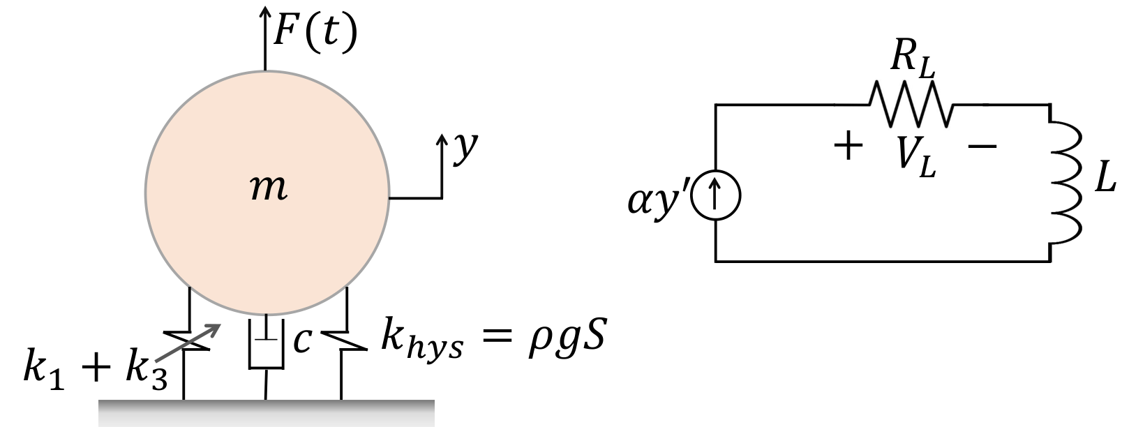
Assuming that the buoy undergoes motions in the heave direction only, the equations governing the motion of the absorber can be obtained by applying Newton’s second law on the buoy, and Kirchhoff’s current law on the harvesting circuit to obtain the following governing equations for the equivalent lumped system shown in Figure 3:

	$\displaystyle\begin{split}&(m+m_{\infty})y^{\prime\prime}+\int_{0}^{t}h(t-\tau)y^{\prime}d\tau+cy^{\prime}+(k_{hys}-k_{1})y+k_{3}y^{3}=f_{wave}\cos(\omega t),\end{split}$			(1a)
		$\displaystyle V_{L}^{{}^{\prime}}+\frac{R_{L}}{L}V_{L}=\alpha y^{\prime}.$		(1b)

Here, $y$ represents the displacement of the buoy in the heave direction and the overprime represents a derivative with respect to time, $t$. In Equation (1a), $m$ and $m_{\infty}$ represent, respectively, the mass of the buoy and the added mass of the fluid. The integral term is used to account for the radiation damping effect; $c$ is a linear viscous damping coefficient; $k_{hys}$ is the stiffness resulting from the hydrostatic buoancy force, which is equal to $\rho gSy$. Here, $\rho$ is the density of water, $g$ is the gravitational acceleration constant, and $S$ is the buoy’s wet surface area. The coefficients $k_{1}>0$ and $k_{3}>0$ represent, respectively, the linear and cubic coefficients of the nonlinear restoring force added to introduce the bi-stable behavior, and $f_{wave}$ and $\omega$ represent, respectively, the wave amplitude and frequency. Note that to induce a bi-stable potential energy function, $k_{1}$ must be larger than $k_{hys}$.

In Equation (1b), $V_{L}$ represents the voltage induced by the generator across a purely resistive load $R_{L}$; $L$ represents the inductance of the harvesting coil, and $\alpha$ is the electromechanical coupling coefficient.

The added mass and the radiation damping depend on the fluid velocity field around the buoy, and hence, are a function of the wave frequency. Following the asymptotic analysis provided in the work of Holme [14] for a spherical buoy of radius $R$, the curves governing the dependence of the normalized added mass denoted here as $\overline{m}_{a}=\frac{m_{a}}{M}$ $(M=\frac{2}{3}\pi R^{3}\rho)$, and the normalized radiation damping coefficient $\overline{B}=\frac{B}{M\omega}$ on the normalized wave frequency $\Omega=\omega/\sqrt{g/R}$ are shown in Figure 4.

The radiation kernel can be further related to the radiation damping coefficient $B(\omega)$ via the following equation [15]:

$$h(t)=\frac{2}{\pi}\int_{0}^{\infty}B(\omega)\cos(\omega t)d\omega,$$

(2)

which can be discretized as following:

$$h(t)=\frac{2}{\pi}\lim_{\delta\omega\to 0}\sum_{i=1}^{\infty}B(\omega_{i})\cos(\omega_{i}t)\delta\omega.$$

(3)

Here, the $B(\omega_{i})$ are the values of the radiation damping coefficient calculated at the discrete value of $\omega_{i}$ shown in Figure 4.

The amplitude of the force $f_{wave}$ acting on the buoy due to the incident waves can be related to the radiation damping coefficients by employing Haskinds’s relation [16, 17], which states that

$$f_{wave}(\omega)=A_{wave}\sqrt{\frac{2\rho g^{3}}{\omega^{3}}B(\omega)},$$

(4)

where $A_{wave}$ is the regular wave amplitude. The physical interpretation of Equation (4) is fairly intuitive, as it relates the tendency of the buoy to radiate waves in a certain direction to the excitation forces the buoy experiences from waves propagating in the same direction. For more insight, the reader can refer to the seminal works of Haskind and Newman[16, 17].

As aforestated, the goal of our work is to obtain approximate analytical solutions of the equations governing the motion of the buoy in order to gain deeper insights into the influence of the shape of the restoring force on the performance of the absorber. To achieve this goal, we will use the method of multiple scales [18]. In order to facilitate the implementation of the method, we obtain in this section an approximation of the convolution integral governing the radiation damping in Equation (1a).

To this end, we first use the fact that the output, $z(t)$, of a linear dynamical system can be expressed as a convolution integral between its input $u(t)$, and an impulse response function $h(t)$, in the form

$$\textbf{z}(t)=\int_{0}^{t}h(t-\tau)\textbf{u}(\tau)d\tau\approx\textbf{C}_{r}\textbf{x}(t).$$

(5)

Here, $\textbf{z(t)}\in\mathbb{R}^{q}$ is the output vector, $\textbf{x(t)}\in\mathbb{R}^{n}$ is the state vector and $\textbf{C}_{r}$ is a $q\times n$ output matrix governed by the following linear state-space equation

$\displaystyle\textbf{x}^{\prime}(t)$

$\displaystyle=\textbf{A}_{r}\textbf{x}(t)+\textbf{B}_{r}\textbf{u}(t).$

(6)

Using the Eigensystem Realization Algorithm (ERA) detailed in Ref. [19], the convolution integral can be expressed in terms of the realized state-space matrices $\textbf{A}_{r},\textbf{B}_{r}$ and $\textbf{C}_{r}$ as:

$$h(t)=\left(M\sqrt{\frac{g}{R}}\right)\textbf{C}_{r}e^{\textbf{A}_{r}t}\textbf{B}_{r},$$

(7)

where the realized state-space matrices are :

$$\textbf{A}_{r}=0.8\begin{pmatrix}-1&1&1\\ -1&0&0\\ -1&0&-2\end{pmatrix},$$

$$\textbf{B}_{r}=\begin{pmatrix}-0.48&-0.02&-0.22\end{pmatrix}^{T},$$

and

$$\textbf{C}_{r}=\begin{pmatrix}-0.46&0&0.18\end{pmatrix}.$$

Note that the numerical values appearing in the realized state-space matrices are general for any spherical buoy of radius, R. For more details on the ERA procedure, the interested reader can refer to Appendix A.

The matrix exponential $e^{\textbf{A}_{r}t}$ in Equation (7) can be further expressed in the following form

$$e^{\textbf{A}_{r}t}=\mathcal{L}^{-1}\left(s\textbf{I}-\textbf{A}_{r}\right)^{-1}.$$

(8)

Here, $\mathcal{L}^{-1}$ is the inverse Laplace transform, and I is the identity matrix. Substituting Equation (8) into Equation (7), we obtain the following analytical expression for $h(t)$:

$$h(t)=\left(M\sqrt{\frac{g}{R}}\right)e^{-\mu t}\left(\lambda_{1}+\lambda_{2}\cos(\mu t)+\lambda_{3}\sin(\mu t)\right),$$

(9)

where $\mu,\lambda_{1},\lambda_{2}$ and $\lambda_{3}$ are constants listed in Table 1, and are valid for any spherical buoy of radius, R.

Figure 5 depicts a comparsion between the analytical expression of $h(t)$ as obtained using Equation (9) and that obtained using the original expression of Equation (3) for a hemispherical buoy of radius $R=5$ [m]. It can be clearly seen that the analytical expression for $h(t)$ is in an excellent agreement with the original impulse response function obtained via Equation (3).

In this subsection, we obtain an approximate solution for Equation (1) when the buoy undergoes motions within a single potential well; i.e, the dynamics around one stable equilibrium node. Upon using the radius of the buoy, $R$, as a length scale and the $\sqrt{g/R}$ as a time scale, we obtain the following dimensionless equivalent equation of motion:

	$\displaystyle\ddot{Y}$	$\displaystyle+\delta_{1}\int_{0}^{t^{*}}\overline{h}(t^{*}-\tau)\dot{Y}(\tau)d\tau+\delta_{2}\dot{Y}-\omega^{2}_{n}Y+\gamma Y^{3}=g_{wave}\cos(\Omega t^{*}),$		(10a)
		$\displaystyle\dot{v}+\theta v=\dot{Y},$		(10b)

where the overdot represents the derivative with respect to the nondimensional time, $t^{*}$, and the other parameters and nondimensional groups are defined as:

$\delta_{1}=\frac{m+m_{\infty}}{M}$, $\delta_{2}=\frac{c}{(m+m_{\infty})}\sqrt{\frac{R}{g}}$, $\omega_{n}=\sqrt{\frac{(k_{1}-\rho gS)R}{(m+m_{\infty})g}}$, $\gamma=\frac{R^{3}k_{3}}{(m+m_{\infty})g}$, $g_{wave}=\frac{AM}{R(m+m_{\infty})}\Omega\sqrt{\frac{3\overline{B}}{\pi}}$ , $M=\frac{2}{3}\pi R^{3}\rho$, $Y=\frac{y}{R}$, $v=\frac{V}{\alpha R}$, $\overline{h}=\frac{h}{M}\sqrt{\frac{R}{g}}$, $\theta=\frac{R_{L}}{L}\sqrt{\frac{R}{g}}$, $t^{*}=t\sqrt{g/R}$.

We expand the dynamics governed by Equation (10) about the stable node, $Y_{s}=\sqrt{\omega^{2}_{n}/\gamma}$, by introducing the transformation $Y(t^{*})=z(t^{*})-Y_{s}$ into Equation (10). This yields

	$\displaystyle\begin{split}\ddot{z}&+\delta_{1}\int_{0}^{t^{*}}\overline{h}(t^{*}-\tau)\dot{z}(\tau)d\tau+\delta_{2}\dot{z}+\omega^{2}_{0}z+\eta z^{2}+\gamma z^{3}=g_{wave}\cos(\Omega t^{*}),\end{split}$			(11a)
		$\displaystyle\dot{v}+\theta v=\dot{z}.$		(11b)

Here $z(t)$ represents the dynamic trajectories within the potential well, $\omega_{o}=\sqrt{2}\omega_{n}$ is the corresponding local frequency of oscillations. It is worth noting that the expansion about the stable node introduces a new quadratic term which captures the asymmetric nature of the motion trajectories about the stable node, $Y_{s}$.

To implement the method of multiple scales on Equation (11), we introduce multiple time scales, $T_{n}=\epsilon^{n}t^{*}$, $n=0,1,2$. It follows that

$$\begin{split}\dot{(.)}&=D_{0}+\epsilon D_{1}+\epsilon^{2}D_{2}+O(\epsilon^{3}),\\ \ddot{(.)}&=D_{0}^{2}+\epsilon^{2}D_{1}+2\epsilon D_{0}D_{1}+2\epsilon^{2}D_{0}D_{2}+O(\epsilon^{3}),\end{split}$$

(12)

where $\epsilon$ is a scaling parameter, and $D_{n}$ is the temporal derivative operator with respect to the time scales, $T_{n}$. Next, we seek an expansion for the response $z(t^{*})$ and voltage $v(t^{*})$ as

	$\displaystyle z(t^{*},\epsilon)$	$\displaystyle=z_{0}(T_{0},T_{1},T_{2})+\epsilon z_{1}(T_{0},T_{1},T_{2})+\epsilon^{2}z_{2}(T_{0},T_{1},T_{2})+O(\epsilon^{3}),$		(13a)
	$\displaystyle v(t^{*},\epsilon)$	$\displaystyle=v_{0}(T_{0},T_{1},T_{2})+\epsilon v_{1}(T_{0},T_{1},T_{2})+\epsilon^{2}v_{2}(T_{0},T_{1},T_{2})+O(\epsilon^{3}).$		(13b)

Based on the typically small values of the damping coefficients, quadratic and cubic nonlinearities, electromechanical coupling, the time constant of the harvesting circuit, and the excitation amplitude, we scale them to be at order $\epsilon^{2}$; that is

$\delta_{1}=\epsilon^{2}\delta_{1}$, $\delta_{2}=\epsilon^{2}\delta_{2}$, $\eta=\epsilon^{2}\eta$, $\gamma=\epsilon^{2}\gamma$ , $g_{wave}=\epsilon^{2}g_{wave}$.

Since large-amplitude intra-well motions occur near the primary resonance of the system; i.e. when $\Omega$ is near $\omega_{o}$, we limit the intra-well analysis to wave frequencies that are close to $\omega_{o}$ by introducing the detuning parameter $\sigma$ such that

$$\Omega=\omega_{o}+\epsilon^{2}\sigma.$$

(14)

Upon substituting Equations (12 - 14) into Equation (11), then collecting terms of equal powers of $\epsilon$, we obtain the following perturbation problems at the different scales:

$O(\epsilon^{0})$:

	$\displaystyle D_{0}^{2}z_{0}+\omega_{o}^{2}z_{0}$	$\displaystyle=0,$		(15a)
	$\displaystyle D_{0}v_{0}+\theta v_{0}$	$\displaystyle=D_{0}z_{0},$		(15b)

$O(\epsilon^{1})$:

	$\displaystyle D_{0}^{2}z_{1}+\omega_{o}^{2}z_{1}$	$\displaystyle=-2D_{0}D_{1}z_{0}-\eta z_{0}^{2},$		(16a)
	$\displaystyle D_{0}v_{1}+\theta z_{1}$	$\displaystyle=D_{0}z_{1}+D_{1}z_{0}-D_{0}v_{0},$		(16b)

$O(\epsilon^{2})$:

	$\displaystyle\begin{split}D_{0}^{2}z_{2}+\omega^{2}_{o}z_{2}=&-2D_{0}D_{1}z_{1}-2D_{0}D_{2}z_{0}-D_{1}^{2}z_{0}-\delta_{1}\int_{0}^{T_{0}}\overline{h}(T_{0}-\tau)D_{0}z_{0}(\tau)d\tau\\ &-\delta_{2}D_{0}z_{0}-2\eta z_{0}z_{1}-\gamma z^{3}_{0}+g_{wave}\cos\left((\omega_{o}+\epsilon^{2}\sigma)T_{0}\right),\end{split}$			(17a)
	$\displaystyle\begin{split}D_{0}v_{2}+\theta v_{2}=&D_{0}z_{2}+D_{2}z_{0}+D_{1}z_{1}-D_{2}v_{0}-D_{1}v_{1}.\end{split}$			(17b)

Upon solving Equations (15) and (16), we obtain the following expressions for $z_{0}$, $v_{0}$, $z_{1}$ and $v_{1}$:

	$\displaystyle z_{0}$	$\displaystyle=A(T_{1},T_{2})e^{i\omega_{o}T_{0}}+cc,$		(18a)
	$\displaystyle v_{0}$	$\displaystyle=\Gamma_{0}A(T_{1},T_{2})e^{i\omega_{o}T_{0}}+cc,$		(18b)

and

	$\displaystyle z_{1}$	$\displaystyle=\frac{\eta}{\omega^{2}_{o}}\left(\frac{A^{2}(T_{1},T_{2})}{3}e^{2i\omega_{o}T_{0}}-2A(T_{1},T_{2})\overline{A}(T_{1},T_{2})\right)+cc,$		(19a)
	$\displaystyle v_{1}$	$\displaystyle=\eta\Gamma_{1}\frac{A^{2}(T_{1},T_{2})}{3\omega_{o}^{2}}e^{2i\omega_{0}T_{0}}+cc,$		(19b)

where

$$\Gamma_{0}=\frac{\omega^{2}_{o}+i\theta\omega_{o}}{\omega^{2}_{o}+\theta^{2}},\qquad\Gamma_{1}=\frac{4\omega^{2}_{o}+2i\theta\omega_{o}}{4\omega^{2}_{o}+\theta^{2}},$$

and $cc$ stands for the complex conjugate of the preceding terms.

Elimination of the secular terms from the second-order perturbation problem, yields $D_{1}A(T_{1},T_{2})=0$, which implies that the complex valued function $A$ is only dependent on the third time scale, $T_{2}$.

Elimination of the secular terms from the third-order problem associated with Equation (17) requires evaluating the convolution integral $\int_{0}^{T_{0}}\overline{h}(T_{0}-\tau)D_{0}z_{0}(\tau)d\tau$. To this end, we use Equation (9) to write:

$$\overline{h}(T_{0}-\tau)=\frac{e^{-\mu T_{0}}}{M}\sqrt{\frac{R}{g}}\Big(\lambda_{1}e^{\mu\tau}+\lambda_{2}e^{\mu\tau}\cos(\mu\tau-\mu T_{0})-\lambda_{3}e^{\mu\tau}\sin(\mu\tau-\mu T_{0})\Big).$$

(20)

Also, from Equation (18), we have

$$D_{0}z_{0}(\tau)=i\omega_{o}Ae^{i\omega_{o}\tau}+cc.$$

(21)

Thus, using Equations (20) and (21), we can express the convolution integral as

$$\begin{split}\int_{0}^{T_{0}}\overline{h}(T_{0}-\tau)D_{0}z_{0}(\tau)d\tau=i\omega_{o}Ae^{-\mu T_{0}}\int_{0}^{T_{0}}\Big(&\lambda_{1}e^{(\mu+i\omega_{o})\tau}+\lambda_{2}e^{(\mu+i\omega_{o})\tau}\cos(\mu\tau-\mu T_{0})\\ &-\lambda_{3}e^{(\mu+i\omega_{o})\tau}\sin(\mu\tau-\mu T_{0})\Big)d\tau,\end{split}$$

(22)

which upon integration by parts yields

$$\int_{0}^{T_{0}}\overline{h}(T_{0}-\tau)D_{0}z_{0}(\tau)d\tau=A\omega_{o}(\xi_{0}+i\bar{\xi}_{0})e^{i\omega_{o}T_{0}}+NST+cc,$$

(23)

where $NST$ stands for non-secular terms, and

$$\begin{split}\xi_{0}&=\left(\frac{\lambda_{1}\omega_{o}}{\mu^{2}+\omega_{o}^{2}}+\frac{2\lambda_{2}\mu^{2}\omega_{o}}{4\mu^{4}+\omega_{o}^{4}}-\frac{\lambda_{3}\omega_{o}^{3}}{4\mu^{4}+\omega_{o}^{4}}\right),\\ \bar{\xi}_{0}&=\left(\frac{\lambda_{1}\mu}{\mu^{2}+\omega_{o}^{2}}+\frac{\lambda_{2}(2\mu^{3}-\mu\omega_{o}^{2})}{4\mu^{4}+\omega_{o}^{4}}-\frac{\lambda_{3}(2\mu^{3}+\mu\omega_{o}^{2})}{4\mu^{4}+\omega_{o}^{4}}\right).\end{split}$$

(24)

Substituting Equations (23) and (24) into the third perturbation problem presented in Equation (17), and using the following polar transformation for the complex valued function $A(T_{2})$

$$\begin{split}A(T_{2})&=\frac{a(T_{2})}{2}e^{i\beta(T_{2})},\\ \overline{A}(T_{2})&=\frac{a(T_{2})}{2}e^{-i\beta(T_{2})},\end{split}$$

(25)

then eliminating the secular terms, yields the following modulation equations:

$$D_{2}a=-\left(\frac{\delta_{1}\bar{\xi}_{0}}{2}+\frac{\delta_{2}}{2}\right)a+\frac{g_{wave}}{2\omega_{o}}\sin\psi$$

(26)

$$aD_{2}\psi=\left(\sigma-\frac{\delta_{1}\xi_{0}}{2}\right)a+\left(\frac{5\eta^{2}}{12\omega_{o}^{3}}-\frac{3\gamma}{8\omega_{o}}\right)a^{3}+\frac{g_{wave}}{2\omega_{o}}\cos\psi,$$

(27)

where $a$ and $\beta$ represent, respectively, the amplitude and phase of oscillations, and $\psi=\sigma T_{2}-\beta$.

In this section, we seek an approximate solution for the high energy orbits; i.e., when the system undergoes global inter-well oscillations. Since Equation (10) has a negative linear stiffness, it is difficult to employ the method of multiple scales in its straightforward fashion. To overcome this, we first expand the natural frequency of symmetric oscillations to be in the following form

$$\omega_{N}^{2}=-\omega_{n}^{2}+\sigma_{1},$$

(28)

where $\sigma_{1}$ is a detuning parameter. Since we are seeking an approximate solution in the vicinity of the primary resonance of the inter-well motions, we express the nearness of the wave frequency to the natural frequency, $\omega_{N}$, by introducing the detuning parameter $\sigma_{2}$, such that

$$\Omega^{2}=\omega_{N}^{2}+\epsilon^{2}\sigma_{2}.$$

(29)

Upon adding Equations (28 - 29), we arrive at

$$-\omega_{n}^{2}=\Omega^{2}-(\omega_{N}^{2}+\omega_{n}^{2})-\epsilon^{2}(\Omega^{2}-\omega_{N}^{2}).$$

(30)

Substituting Equation (30) into Equation (10), we obtain

$$\begin{split}\ddot{Y}+&\epsilon^{2}\delta_{1}\int_{0}^{t^{*}}h(t^{*}-\tau)\dot{Y}(\tau)d\tau+\epsilon^{2}\delta_{2}\dot{Y}+\Omega^{2}Y\\ +&\epsilon(-(\omega_{N}^{2}+\omega_{n}^{2})Y+\gamma Y^{3})-\epsilon^{2}(\Omega^{2}-\omega_{N}^{2})Y=\epsilon^{2}g_{wave}\cos(\Omega t^{*}).\end{split}$$

(31)

Next, we employ the method of multiple scales on Equation (31) by introducing slow and fast time scales $T_{n}=\epsilon^{n}t^{*}$, $n=0,1,2$, and seek an expansion of the response in the form

	$\displaystyle Y(t^{*},\epsilon)$	$\displaystyle=Y_{0}(T_{0},T_{1},T_{2})+\epsilon Y_{1}(T_{0},T_{1},T_{2})+\epsilon^{2}Y_{2}(T_{0},T_{1},T_{2})+O(\epsilon^{3}),$		(32a)
	$\displaystyle v(t^{*},\epsilon)$	$\displaystyle=v_{0}(T_{0},T_{1},T_{2})+\epsilon v_{1}(T_{0},T_{1},T_{2})+\epsilon^{2}v_{2}(T_{0},T_{1},T_{2})+O(\epsilon^{3}).$		(32b)

Implementing the method of multiple scales on the scaled equations as described in the previous subsection yields the following solution for $Y$ and $v$.

	$\displaystyle Y$	$\displaystyle=a\cos(\Omega t^{*}+\psi)+O(\epsilon),$		(33a)
	$\displaystyle v$	$\displaystyle=\Gamma_{2}a\cos(\Omega t^{*}+\psi)+O(\epsilon),$		(33b)

where

$$\Gamma_{2}=\frac{\Omega^{2}+i\theta\Omega}{\Omega^{2}+\theta^{2}}$$

and the amplitude, $a$, and phase, $\psi$, of the response are governed by the following modulation equations:

$$\omega_{n}D_{2}a=-\left(\frac{\omega_{n}\delta_{1}\bar{\xi_{1}}+\omega_{n}\delta_{2}}{2}\right)a-\frac{f_{wave}}{2}\sin\psi$$

(34)

$$\omega_{n}aD_{2}\psi=-\left(\frac{\Omega^{2}+\omega_{n}^{2}}{2}-\omega_{n}\delta_{1}\xi_{1}\right)a+\frac{3\gamma}{8}a^{3}+\frac{3\gamma^{2}}{256\omega_{n}^{2}}a^{5}-\frac{f_{wave}}{2}\cos\psi,$$

(35)

where

$$\begin{split}\xi_{1}&=\left(\frac{\lambda_{1}\omega_{n}}{\mu^{2}+\omega_{n}^{2}}+\frac{2\lambda_{2}\mu^{2}\omega_{n}}{4\mu^{4}+\omega_{n}^{4}}-\frac{\lambda_{3}\omega_{n}^{3}}{4\mu^{4}+\omega_{n}^{4}}\right)\\ \bar{\xi}_{1}&=\left(\frac{\lambda_{1}\mu}{\mu^{2}+\omega_{n}^{2}}+\frac{\lambda_{2}(2\mu^{3}-\mu\omega_{n}^{2})}{4\mu^{4}+\omega_{n}^{4}}-\frac{\lambda_{3}(2\mu^{3}+\mu\omega_{n}^{2})}{4\mu^{4}+\omega_{n}^{4}}\right)\end{split}$$

(36)

The long-time steady-state behavior of the absorber is of particular interest to assess its performance. Thus, the time derivatives in Equations (26 - 27) and (34 - 35) are set to zero and the resulting algebraic equations are then solved numerically for the steady-state amplitude $a_{o}$, and phase $\psi_{o}$. For intra-well oscillations, we obtain:

	$\displaystyle\begin{split}Y=a_{o}\cos(\Omega t^{*}-\psi_{o})+\frac{\eta}{2\omega_{0}^{2}}\left(-a_{o}^{2}+\frac{a_{o}^{2}}{3}\cos(2\Omega t^{*}-2\psi_{o})\right)+O(\epsilon^{2}),\end{split}$			(37a)
		$\displaystyle v=\frac{\omega_{0}^{2}}{\omega_{0}^{2}+\theta^{2}}a_{o}\cos(\Omega t^{*}-\psi_{o})-\frac{\omega_{0}\theta}{\omega_{0}^{2}+\theta^{2}}a_{o}\sin(\Omega t^{*}-\psi_{o})+O(\epsilon^{2}),$		(37b)

and for the inter-well oscillations, we obtain

	$\displaystyle\begin{split}Y&=a_{o}\cos(\Omega t^{*}-\psi_{o})+\left(\frac{\gamma}{32\omega_{n}^{2}}a_{o}^{3}+\frac{3\gamma^{2}}{1024\omega_{n}^{4}}a_{o}^{5}\right)\cos(3\Omega t^{*}-3\psi_{o})\\ &+\frac{\gamma^{2}}{1024\omega_{n}^{4}}a_{o}^{5}\cos(5\Omega t^{*}-5\psi_{o})+O(\epsilon^{2}),\end{split}$			(38a)
	$\displaystyle v$	$\displaystyle=\frac{\omega_{n}^{2}}{\omega_{n}^{2}+\theta^{2}}a_{o}\cos(\Omega t^{*}-\psi_{o})-\frac{\omega_{n}\theta}{\omega_{n}^{2}+\theta^{2}}a_{o}\sin(\Omega t^{*}-\psi_{o})+O(\epsilon^{2}).$		(38b)

Using the steady-state response, the average power available at the buoy can be expressed as

$$P_{avg}=\frac{1}{T^{*}}\int_{0}^{T^{*}}\delta_{2}\dot{Y}^{2}dt^{*},$$

(39)

where $T^{*}$ is the period of oscillations. For intra-well oscillations Equation (39) reduces to

$$P_{avg}=\delta_{2}\left(\frac{\Omega^{2}a_{o}^{2}}{2}+\frac{\eta^{2}\Omega^{2}a_{o}^{4}}{18\omega_{0}^{4}}\right)+O(\epsilon^{2}),$$

(40)

while for inter-well oscillations, we get

$$P_{avg}=\delta_{2}\left(\frac{\Omega^{2}a_{o}^{2}}{2}+\frac{9\gamma^{2}\Omega^{2}a_{o}^{6}}{2048\omega_{n}^{4}}\right)+\ O(\epsilon^{2}).$$

(41)

In addition to the averaged power, we are also interested in evaluating the capture width ratio (CWR), which is a common parameter used to evaluate a PWA’s performance. CWR or absorption width as commonly coined in some literature is defined as the ratio between the average absorbed power, $P_{avg}$, and the power available at the wave front, $P_{wave}$. The latter can be obtained by multiplying the wave energy flux per unit crest length with the buoy’s characteristic length, which is the diameter for a hemispherical buoy. This yields [20]:

$$CWR=\frac{6(m+m_{\infty})\Omega}{\rho RA^{2}}P_{avg}.$$

(42)

The cyclic-fold point $C_{f1}$ satisfies the relation $d\Omega/da_{o}=0$ on the resonant branch, $B_{L}$. Thus, its location can be obtained by differentiating Equations (34-35) with respect to $a_{o}$ and setting $d\Omega/da_{o}$ to zero to arrive at the following 8^th order polynomial:

		$\displaystyle\frac{45\gamma^{4}}{4096\omega_{n}^{4}}a_{b}^{8}+\frac{9\gamma^{3}}{128\omega_{n}^{2}}a_{b}^{6}+\left(\frac{99\gamma^{2}}{64}-\frac{3\gamma^{2}\Omega_{b}^{2}}{128\omega_{n}^{2}}+\frac{3\gamma^{2}\delta_{1}\xi_{1}}{64\omega_{n}}\right)a_{b}^{4}-3\gamma\left(\Omega_{b}^{2}+\omega_{n}^{2}-\delta_{1}\omega_{n}\xi_{1}\right)a_{b}^{2}$		(43)
		$\displaystyle+\left(\Omega_{b}^{2}+\omega_{n}^{2}-\delta_{1}\omega_{n}\xi_{1}\right)^{2}+\left(\delta_{2}\omega_{n}+\delta_{1}\omega_{n}\bar{\xi}_{1}\}\right)^{2}=0.$

where $(\Omega_{b},a_{b})$ represent the wave frequency and response amplitude at which the bifurcation occurs. For any set of design parameters, the polynomial in Equation (43) can be solved to obtain the locus of the $Cf_{1}$ bifurcation in the parameter space of wave amplitude and frequency.

These cyclic fold bifurcations also satisfy the relation $d\Omega/da_{o}=0$ but on the intra-well branch, $B_{n}$; i.e. Equations (26-27). Differentiating Equations (26-27) with respect to $a_{o}$ and setting $d\Omega/da_{o}=0$, we obtain

$$a_{b}^{2}=\frac{-2\left(\Omega_{b}-\omega_{o}-\frac{\delta_{1}\xi_{0}}{2}\right)\pm\sqrt{\left(\Omega_{b}-\omega_{o}-\frac{\delta_{1}\xi_{0}}{2}\right)^{2}-3\left(\frac{\delta_{1}\bar{\xi}_{0}}{2}+\frac{\delta_{2}}{2}\right)^{2}}}{3\left(\frac{5\eta^{2}}{12\omega_{o}^{3}}-\frac{3\gamma}{8\omega_{o}}\right)}.$$

(44)

Here, $a_{b}$ and $\Omega_{b}$ are, respectively, the amplitude of oscillations and the wave frequency at which the cyclic-fold bifurcations, $Cf_{2}$ and $Cf_{3}$, occurs. Upon solving Equation (44), we can obtain the loci of the $Cf_{2}$ and $Cf_{3}$ bifurcations in the parameter space of wave amplitude and frequency.

One of the main dynamical characteristics of the intra-well oscillations is the appearance of a period-doubling bifurcation on the $B_{r}$ branch as the wave frequency is decreased toward lower values. To estimate this bifurcation point as function of the wave frequency and amplitude, we perturb the periodic orbit ${Y}(t^{*})$ by introducing the perturbation $\mathcal{p(t^{*})}$ such that

$$\tilde{Y}(t^{*})=Y(t^{*})+\mathcal{p(t^{*})}.$$

(45)

Here, $\tilde{Y}(t^{*})$ is a stable periodic orbit if $\mathcal{p(t^{*})\to 0}$ as $t^{*}\to\infty$; otherwise it is unstable. Substituting Equation (45) into Equation (11) and retaining only linear terms in $\mathcal{p(t^{*})}$, we obtain, after simplifications, the following scaled equations:

$$\begin{split}\mathcal{p}^{\prime\prime}+\epsilon\delta_{1}\int_{0}^{t^{*}}\overline{h}(t^{*}-\tau)\mathcal{p}^{\prime}(\tau)d\tau+\epsilon\delta_{2}\mathcal{p}^{\prime}&+[G_{0}+\epsilon G_{1}\cos(\Omega t^{*}-\psi)+\epsilon^{2}G_{2}\cos(2\Omega t^{*}-2\psi)\\ &+\epsilon^{2}G_{3}\cos(3\Omega t^{*}-3\psi)+\epsilon^{2}G_{4}\cos(4\Omega t^{*}-4\psi)]\mathcal{p}=0,\end{split}$$

(46)

where Equation (46) represents a Mathieu’s-type differential equation with four parametric excitation terms. Each of these terms produces a principle subharmonic parametric instability when their frequency is half the natural frequency $\sqrt{G_{0}}$ of the perturbation [21, 22]. The interested reader can refer to Appendix B for the full expressions of the parametric terms constants, $G_{i}$.

References

- [1] Elie Al Shami, Ran Zhang, and Xu Wang. Point absorber wave energy harvesters: A review of recent developments. Energies, 12(1):47, 2019.
- [2] Johannes Falnes and Jørgen Hals. Heaving buoys, point absorbers and arrays. Philosophical Transactions of the Royal Society A: Mathematical, Physical and Engineering Sciences, 370(1959):246–277, January 2012.
- [3] Benjamin Drew, Andrew R Plummer, and M Necip Sahinkaya. A review of wave energy converter technology. Proceedings of the Institution of Mechanical Engineers, Part A: Journal of Power and Energy, 223(8):887–902, 2009.
- [4] Davood Younesian and Mohammad-Reza Alam. Multi-stable mechanisms for high-efficiency and broadband ocean wave energy harvesting. Applied energy, 197:292–302, 2017.
- [5] Benjamin W Schubert, William SP Robertson, Benjamin S Cazzolato, Mergen H Ghayesh, and Nataliia Y Sergiienko. Performance enhancement of submerged wave energy device using bistability. Ocean Engineering, 213:107816, 2020.
- [6] Mohammed F Daqaq, Ravindra Masana, Alper Erturk, and D Dane Quinn. On the role of nonlinearities in vibratory energy harvesting: a critical review and discussion. Applied Mechanics Reviews, 66(4), 2014.
- [7] Ru Xi, Haicheng Zhang, Huai Zhao, Ramnarayan Mondal, et al. High-performance and robust bistable point absorber wave energy converter. Ocean Engineering, 229:108767, 2021.
- [8] Xiaolong Xiao, Longfei Xiao, and Tao Peng. Comparative study on power capture performance of oscillating-body wave energy converters with three novel power take-off systems. Renewable Energy, 103:94–105, 2017.
- [9] Haicheng Zhang, Ru Xi, Daolin Xu, Kai Wang, Qijia Shi, Huai Zhao, and Bo Wu. Efficiency enhancement of a point wave energy converter with a magnetic bistable mechanism. Energy, 181:1152–1165, 2019.
- [10] Xian-tao Zhang, Jian-min Yang, and Long-fei Xiao. An oscillating wave energy converter with nonlinear snap-through power-take-off systems in regular waves. China Ocean Engineering, 30(4):565–580, 2016.
- [11] Xiantao Zhang, Xinliang Tian, Longfei Xiao, Xin Li, and Lifen Chen. Application of an adaptive bistable power capture mechanism to a point absorber wave energy converter. Applied Energy, 228:450–467, 2018.
- [12] Xiantao Zhang, XinLiang Tian, Longfei Xiao, Xin Li, and Wenyue Lu. Mechanism and sensitivity for broadband energy harvesting of an adaptive bistable point absorber wave energy converter. Energy, 188:115984, 2019.
- [13] Yang Song, Xiaoxian Guo, Hongchao Wang, Xinliang Tian, Handi Wei, and Xiantao Zhang. Performance analysis of an adaptive bistable point absorber wave energy converter under white noise wave excitation. IEEE Transactions on Sustainable Energy, 2020.
- [14] A Hulme. The wave forces acting on a floating hemisphere undergoing forced periodic oscillations. Journal of Fluid Mechanics, 121:443–463, 1982.
- [15] T Francis Ogilvie and Ernest O Tuck. A rational strip theory of ship motions: part i. Technical report, University of Michigan, 1969.
- [16] MD Haskind. The exciting forces and wetting of ships in waves. report, 2010.
- [17] John Nicholas Newman. The exciting forces on fixed bodies in waves. Journal of ship research, 6(04):10–17, 1962.
- [18] Ali H Nayfeh. Perturbation methods. John Wiley & Sons, 2008.
- [19] Steven L Brunton and J Nathan Kutz. Data-driven science and engineering: Machine learning, dynamical systems, and control. Cambridge University Press, 2019.
- [20] Liguo Wang. Modelling and advanced control of fully coupled wave energy converters subject to constraints: the wave-to-wire approach. PhD thesis, Acta Universitatis Upsaliensis, 2017.
- [21] Robert A Meyers. Mathematics of complexity and dynamical systems. Springer Science & Business Media, 2011.
- [22] Ivana Kovacic, Richard Rand, and Si Mohamed Sah. Mathieu’s equation and its generalizations: overview of stability charts and their features. Applied Mechanics Reviews, 70(2), 2018.