Eigenvalues and spectral gap in sparse random simplicial complexes

Shaked Leibzirer and Ron Rosenthal Thanks: Partially supported by ISF 771/17 and BSF grant 2018330.

Abstract

We consider the adjacency operator $A$ of the Linial-Meshulam model $X(d,n,p)$ for random $d-$ dimensional simplicial complexes on $n$ vertices, where each $d-$ cell is added independently with probability $p\in[0,1]$ to the complete $(d-1)$ -skeleton. We consider sparse random matrices $H$ , which are generalizations of the centered and normalized adjacency matrix $\mathcal{A}:=(np(1-p))^{-1/2}\cdot(A-\mathbb{E}\left[A\right])$ , obtained by replacing the Bernoulli $(p)$ random variables used to construct $A$ with arbitrary bounded distribution $Z$ . We obtain bounds on the expected Schatten norm of $H$ , which allow us to prove results on eigenvalue confinement and in particular that $\left\|H\right\|_{2}$ converges to $2\sqrt{d}$ both in expectation and $\mathbb{P}-$ almost surely as $n\to\infty$ , provided that $\mathrm{Var}(Z)\gg\frac{\log n}{n}$ . The main ingredient in the proof is a generalization of [LVHY18, Theorem 4.8] to the context of high-dimensional simplicial complexes, which may be regarded as sparse random matrix models with dependent entries.

1 Introduction

The Erdős–Rényi graph ([ER59, ER61]) $G\left(n,p\right)$ , is a random graph on $n$ vertices, where each edge is added independently with probability $p\in\left[0,1\right]$ that might depend on $n$ . The model and particularly the spectrum of its adjacency matrix $A$ has been extensively studied. For insteance, it follows from Wigner’s semicircle theorem that the spectrum of $(np(1-p))^{-1/2}(A-\mathbb{E}[A])$ converges weakly in probability to the semicircle law, provided $\lim_{n\to\infty}np(1-p)=\infty$ , and it is shown in [FK81, Vu07] that under the assumption $np\gg\log^{4}\left(n\right),$ namely $\lim_{n\to\infty}(np)^{-1}\log^{4}\left(n\right)=0$ , one has

\mathbb{E}\left[\frac{\left\|A-\mathbb{E}\left[A\right]\right\|}{\sqrt{np}}\right]\leq 2\left(1+o\left(1\right)\right),\qquad\text{ as $n\to\infty$,}

(1.1)

which is a well-known result regarding the spectral gap of the adjacency matrix of the homogeneous Erdős–Rényi graph. Recently, it was shown independently in [BGBK20] and [LVHY18] that (1.1) holds under the weaker assumption $np(1-p)\gg\log\left(n\right)$ , which by [BGBK20, BGBK19, ADK21] is the optimal regime.

The Linial-Meshulam model, c.f. [LM06, MW09], is a high-dimensional generalization of the Erdős–Rényi model. Given $n,d\in\mathbb{N}$ such that $n\geq d+1$ , and $p\in\left[0,1\right]$ that might depend on $n$ , the Linial-Meshulam model $X\equiv X\left(d,n,p\right)$ , is a random $d$ -dimensional simplicial complex on $n$ vertices with a complete $(d-1)$ -skeleton, in which each $d$ -cell is added to $X$ independently with probability $p$ . When $d=1$ , the model reduces to the Erdős–Rényi random graph. Since its appearance the Linial-Meshulam model attracted much attention, see for example [MW09, Koz10, BHK11, Wag11, HJ13, ALLuM13, CCFK16, GW16, LP16, KR17, HS17, PR17, HKP17, CDGKS18, ŁP18, LP19, HK19, FP20, LP22].

Let $A$ be the adjacency operator associated with the Linial-Meshulam model $X\equiv X(d,n,p)$ , see Section 2 for a precise definition. In this paper we consider a random matrix $H$ which is a generalization of the centered and normalized adjacency matrix, defined by $\mathcal{A}:=\left(np\left(1-p\right)\right)^{-\frac{1}{2}}\left(A-\mathbb{E}\left[A\right]\right)$ , where the Bernoulli $(p)$ random variables used to construct $A$ are replaced with an arbitrary bounded distribution $Z$ . The matrix $H$ is a sparse self-adjoint random matrix equipped with the same dependent structure as $\mathcal{A}$ , and in particular its entries are only independent (up to the self-adjointness constraint) if and only if $d=1$ (see [KR17] for further details).

Our main result is a generalization of (1.1) to random matrices of type $H$ and in particular to the rescaled and centered adjacency matrix $\mathcal{A}$ of random simplicial complexes $X(d,n,p)$ . Previous results related to the spectrum of the adjacency matrix $A$ for arbitrary $d\in\mathbb{N}$ were introduced in [KR17] and [GW16]. In [KR17, Theorem 5.1], the authors assume $np(1-p)\gg\log^{4}\left(n\right)$ and at the cost of this stronger assumption (compared to $np(1-p)\gg\log\left(n\right)$ ) establish (1.1), for all $d\geq 2$ with the appropriate optimal bound in the right hand side of (1.1). On the other hand, in [GW16, Theorem 2], it is shown that under the assumption $np(1-p)\gg\log\left(n\right)$ , one can obtain an upper bound on the left hand side of (1.1), which is not optimal. In [LVHY18], a key ingredient in problem the proof of (1.1) for the Erdős–Rényi model, namely the case $d=1$ is [LVHY18, Theorem 4.8], which assumes independent entries (up to self-adjointness). Due to the dependent structure of the entries of $H$ , one can not apply [LVHY18, Theorem 4.8] whenever $d>1$ . In this paper, we generalize [LVHY18, Theorem 4.8] to random matrices of type $H$ (see Theorem 2.1), which allows us to obtain bounds on the $2k-$ Schatten norm

\mathbb{E}\left[\left\|H\right\|_{S_{2k}}\right]:=\mathbb{E}\bigg[\sqrt[2k]{\text{Trace}\left(\left|H\right|^{2k}\right)}\bigg]\,,

for all $d\geq 1$ , where $\left|H\right|=\sqrt{H^{*}H}$ . Furthermore, we use this bound in order to show that $\lim_{n\to\infty}\mathbb{E}[\left\|H\right\|_{2}]=2\sqrt{d}$ , provided $\text{Var}\left(Z\right)\gg n^{-1}\log n$ , which by [KR17] is the optimal bound. We thus derive the optimal bound achieved in [KR17] under weaker assumptions, which coincide with those postulated in [GW16, LM06, MW09]. In addition to the norm bound, we improve the bound on $\mathbb{P}(\left\|H\right\|_{2}>2\sqrt{d}+\varepsilon)$ obtained in [KR17, Theorem 5.1] for $\varepsilon>0$ . We conclude this section with a few words about the proof of Theorem 2.1. The proof is based on the simplicial structure of the entries of $H$ . Te structure allow us to translate the problem into a combinatorial one by associating a simplicial complex with an embedded path with each of the elements in the sum defining $\text{Trace}(\left|H\right|^{2k})$ . The simplicial structure brings into play new phenomena regarding the relation between the path and the simplicial complexes that do not arise in the graph case, and in particular is not entirely local. Thus new ideas are required, see Lemma 4.8 and Lemma 4.9 for further details.

2 Preliminaries and results

A finite simplicial complex $X$ on a vertex set $V$ is a finite collection of subsets of $V$ that is closed under taking subsets. Namely, if $\tau\in X$ and $\sigma\subseteq\tau$ , then $\sigma\in X$ . The elements of $X$ are called cells, and the dimension of a cell $\tau$ , is defined as $\dim(\tau):=\left|\tau\right|-1$ . For $j\geq-1$ , $X^{j}$ denotes the set of cells of dimension $j$ , which we refer to as $j$ -cells. The dimension of the complex $X$ , denoted by $d$ , is defined as $d:=\max_{\tau\in X}\dim(\tau)$ . For $\ell<d$ , the $\ell$ -skeleton of $X$ is the simplicial complex that consists of all cells of dimension $\leq\ell$ in $X$ . The complex $X$ is said to have a full $\ell$ -dimensional skeleton if its $\ell$ -skeleton contains all subsets of $X^{0}\subset V$ of size $\leq$ $\ell+1$ . Throughout the paper we assume that $X$ has a full $\left(d-1\right)$ -skeleton and that $X^{0}=V$ .

For $j\geq 1$ , every $j$ -cell $\sigma=\left\{\sigma^{0},\ldots,\sigma^{j}\right\}$ has two possible orientations, corresponding to the possible orderings of its vertices, up to an even permutation. Denote an oriented cell by square brackets, and a flip of orientation by an overline. For example, one orientation of $\sigma=\left\{x,y,z\right\}$ is $\left[x,y,z\right]=\left[y,z,x\right]=\left[z,x,y\right]$ . The other orientation is $\overline{\left[x,y,z\right]}=\left[y,x,z\right]=\left[x,z,y\right]=\left[z,y,x\right]$ . Denote by $X_{\pm}^{j}$ the set of oriented $j$ -cells (observe that $|X_{\pm}^{j}|=2\left|X^{j}\right|$ for $j\geq 1$ ) and set $X_{\pm}^{0}=X^{0}$ . Given two oriented cells $\sigma,\sigma^{\prime}\in X_{\pm}^{d-1},$ let $\sigma\cup\sigma^{\prime}$ and $\sigma\cap\sigma^{\prime}$ denote the union and intersection of the corresponding unoriented cells.

Define the boundary $\partial\sigma$ of the $\left(j+1\right)$ -cell $\sigma=\left\{\sigma^{0},\ldots,\sigma^{j+1}\right\}\in X^{j+1}$ as the set of $j-$ cells obtained by omitting the $i$ -th vertex from $\sigma$ , for every $0\leq i\leq j+1$ . Namely,

\partial\sigma=\left\{\left\{\sigma^{0},\ldots,\sigma^{i-1},\sigma^{i+1},\ldots,\sigma^{j+1}\right\}\,:\,0\leq i\leq j+1\right\}\subseteq X^{j}.

An oriented $\left(j+1\right)$ -cell $\left[\sigma^{0},\ldots,\sigma^{j+1}\right]\in X_{\pm}^{j+1}$ induces orientations on the $j$ -cells in its boundary, as follows: the cell $\left\{\sigma^{0},\ldots,\sigma^{i-1},\sigma^{i+1},\ldots,\sigma^{j+1}\right\}$ is oriented as $\left(-1\right)^{i}\left[\sigma^{0},\ldots,\sigma^{i-1},\sigma^{i+1},\ldots,\sigma^{j+1}\right]$ , where $-\sigma:=\overline{\sigma}$ . As introduced in [PR17] one can define a neighboring relation on $X_{\pm}^{j}$ , where $\sigma,\sigma^{\prime}\in X_{\pm}^{j}$ are called neighbors, denoted $\sigma\sim\sigma^{\prime}$ , if there exists an oriented $\left(j+1\right)$ -cell, $\tau\in X_{\pm}^{j+1}$ , such that both $\sigma$ and $\overline{\sigma^{\prime}}$ are in the boundary of $\tau$ as oriented cells (see Figure 2.1 for illustration in the case $d=2$ ). Observe that this definition guarantees that for each pair $\left(\sigma,\sigma^{\prime}\right)\in X^{j}\times X^{j}$ satisfying $\sigma\cup\sigma^{\prime}\in X^{j+1}$ , either $\sigma\sim\sigma^{\prime}$ or $\sigma\sim\overline{\sigma^{\prime}}$ , but not both.

Refer to caption — Figure 2.1: On the left: an oriented $2$ -cell and the orientation it induces on its boundary. On the right: an oriented $1$ -cell in a $2$ -cell together with its two oriented neighboring $1$ -cells.

Let $K^{d}:=K\left(d,n\right)$ be the complete $d$ -complex with vertex set $V=[n]:=\left\{1,2,\ldots,n\right\}$ . That is to say that $K^{d}$ consists of all subsets of $[n]$ of size $\leq d+1$ .

The Linial-Meshulam model $X=X\left(d,n,p\right)$ , with $n,d\in\mathbb{N}$ satisfying $n\geq d+1$ and $p=p\left(n\right)\in\left[0,1\right]$ , is a random $d$ -dimensional simplicial complex on $n$ vertices, with a complete $\left(d-1\right)$ -skeleton in which each $d$ -cell of $K^{d}$ is added to $X$ independently with probability $p$ .

We fix an arbitrary choice of orientation of the $\left(d-1\right)$ -cells in the complete complex, and denote it as $K_{+}^{d-1}\subset K_{\pm}^{d}$ . Observe that this choice of orientation determine the orientation of the elements in $X^{d-1}$ since $X^{d-1}=K^{d-1}$ . Note that there is a natural bijection between $K_{+}^{d-1}$ and $K^{d-1}$ , and hence also between $X_{+}^{d-1}$ and $X^{d-1}$ .

The adjacency matrix $A$ , associated to the random complex $X$ , is a $|X_{+}^{d-1}|\times|X_{+}^{d-1}|$ random matrix, defined via

A_{\sigma\sigma^{\prime}}=\begin{cases}1&\text{if $\sigma\overset{X}{\sim}\sigma^{\prime}$}\\ -1&\text{if $\sigma\overset{X}{\sim}\overline{\sigma^{\prime}}$}\\ 0&\text{otherwise}\end{cases},\qquad\forall\sigma,\sigma^{\prime}\in X_{+}^{d-1}.

Our main result concerns a natural generalization of the centered and normalized adjacency matrix of $A$ , defined by

H_{\sigma\sigma^{\prime}}:=\begin{cases}\frac{Z_{\tau}-\mathbb{E}\left[Z\right]}{\sqrt{n\text{Var}\left(Z\right)}}&\text{if }\sigma\overset{K^{d}}{\sim}\sigma^{\prime}\text{ and $\sigma\cup\sigma^{\prime}=\tau$}\\ -\frac{Z_{\tau}-\mathbb{E}\left[Z\right]}{\sqrt{n\text{Var}\left(Z\right)}}&\text{if }\sigma\overset{K^{d}}{\sim}\overline{\sigma^{\prime}}\text{ and $\sigma\cup\sigma^{\prime}=\tau$}\\ 0&\text{otherwise}\end{cases},\qquad\forall\sigma,\sigma^{\prime}\in X_{+}^{d-1},

where $Z$ is a bounded random variable with positive variance and $\left(Z_{\tau}\right)_{\tau\in K^{d}}$ are i.i.d. copies of it.

Remark.

The results stated below for the matrix $H$ hold also for the unsigned version of the matrix

\tilde{H}_{\sigma\sigma^{\prime}}=\begin{cases}\frac{Z_{\sigma\cup\sigma^{\prime}}-\mathbb{E}\left[Z\right]}{\sqrt{n\text{Var}\left(Z\right)}}&\text{if }\sigma\cup\sigma^{\prime}\in X^{d}\\ 0&\text{otherwise}\end{cases},\qquad\forall\sigma,\sigma^{\prime}\in X_{+}^{d-1}.

(2.1)

Observe that by choosing $Z$ to be a Bernoulli random variable with parameter $p$ , the matrix $H$ reduces to the centered and normalized adjacency matrix of $X$ , defined by

\mathcal{A}:=\frac{1}{\sqrt{nq}}\left(A-\mathbb{E}\left[A\right]\right),

where

q:=q(n)=p(1-p).

Recall that for a square matrix $M\in\mathbb{R}^{n\times n}$ and $p\geq 1$ , the $p-$ Schatten norm of $M$ is defined via

\left\|M\right\|_{S_{p}}=\sqrt[p]{\text{Trace}\left(\left|M\right|^{p}\right)},

where $\left|M\right|=\sqrt{MM^{*}}$ .

We now state our main result.

Theorem 2.1.

For every $d\in\mathbb{N}$ , there exist constants $C_{d},c_{d}\in(0,\infty)$ depending only on $d$ , such that for every $n\geq d+1$ and any integer $k:=k\left(n\right)\geq d$

\sqrt[2k]{\mathbb{E}\left[\left\|H\right\|_{S_{2k}}^{2k}\right]}\leq\Phi\left(\theta_{k},\theta_{k}^{*}\right),

where

\theta_{k}:=\sqrt{\frac{n-d}{n}}{n\choose d}^{\frac{1}{2k}}\qquad,\qquad\theta_{k}^{*}:=\left\|Z_{\tau}-\mathbb{E}\left[Z\right]\right\|_{\infty}\left({n\choose d}\cdot\frac{d\left(n-d\right)}{\left(n\text{Var}\left(Z\right)\right)^{k}}\right)^{\frac{1}{2k}},

and

\Phi\left(x,y\right):=\sqrt[2k]{d!d}\cdot y\left(\frac{x}{y}+2\sqrt{k}\right)^{\frac{d-1}{k}}\left(2\sqrt{d}\left(\frac{x}{y}+2\sqrt{k}\right)+C_{d}\left(\frac{x}{y}+2\sqrt{k}\right)^{\frac{2}{3}}\Big(\log\left(\frac{x}{y}+2\sqrt{k}\right)\Big)^{2/3}+c_{d}\sqrt{k}\right).

Theorem 2.1 allows us to control the operator norm of $H$ .

Corollary 2.2.

For every $d\in\mathbb{N}$ , if $n\text{Var}\left(Z\right)\gg\log\left(n\right)$ , namely $\lim_{n\to\infty}\frac{\log(n)}{n\text{Var}(Z)}=0$ , then

\lim_{n\to\infty}\mathbb{E}\left[\left\|H\right\|_{2}\right]=2\sqrt{d}.

Furthermore, it provides an upper bound on the probability that the operator norm of $H$ is bigger than $2\sqrt{d}$ .

Corollary 2.3.

For every $d\in\mathbb{N}$ , there exists a constant $C_{d}\in(0,\infty)$ , depending only on $d$ , such that if $n\text{Var}\left(Z\right)\gg\log\left(n\right)$ , then for all $\varepsilon>0$ and all large enough $n$ (depending only on $\varepsilon$ and $d$ )

\mathbb{P}\left(\left\|H\right\|_{2}\geq 2\sqrt{d}+\varepsilon\right)\leq e^{-C_{d}n\text{Var}\left(Z\right)\varepsilon^{2}},

and hence

\lim_{n\to\infty}\left\|H\right\|_{2}=2\sqrt{d},\qquad\mathbb{P}\text{-a.s.}

Finally, following the argument in [KR17, Theorem 2.1 and Corollary 2.3] and using Corollary 2.3 allow us to extend the spectral gap result obtained in [KR17] for the matrix $A$ in the regime $nq\gg\log^{4}(n)$ , to the regime $nq\gg\log(n)$ .

Theorem 2.4 (Eigenvalue confinement).

For every $d\geq 2$ , there exists a positive constant $C>0$ depending only on $d$ , such that the following holds with probability at least $1-n^{-D}$ for all $D>0$ , provided $nq\gg\log\left(n\right)$ .

1.

For every $\xi>0$ , and all large enough $n$ (depending on $D$ , $\xi$ and $d$ ), the ${n-1\choose d}$ smallest eigenvalues of the matrix $A$ are within the interval $\sqrt{dnq}\left[-2-\xi,2+\xi\right]$ .
2.

If $q\log^{6}\left(n\right)\leq\frac{1}{C\left(1+D\right)^{6}}$ , then for all large enough $n$ (depending on $D$ and $d$ ), the remaining ${n-1\choose d-1}$ eigenvalues of $A$ lie in the interval $nq+\left[-7d,7d\right]$ .

As an immediate corollary from the last theorem we obtain

Corollary 2.5 (Spectral gap).

For every $d\geq 2$ , there exists a positive constant $C>0$ depending only on $d$ such that for all $\xi>0$ , $D>0$ satisfying $nq\gg\log\left(n\right)$ and $q\log^{6}\left(n\right)\leq\frac{1}{C\left(1+D\right)^{6}}$ , we have for all $n$ large enough (depending on $d$ , $D$ and $\xi$ )

\lambda_{{n-1\choose d}+1}-\lambda_{{n-1\choose d}}=nq-2\sqrt{dnq}\left(1+O\left(\xi\right)\right),

with probability at least $1-n^{-D}$ .

Conventions. Throughout the rest of the paper we use $C$ to denote a generic large positive constant, which may depend on some fixed parameters and whose value may change from one expression to the next. If $C$ depends on some parameter $k$ , we sometimes emphasize this dependence by writing $C_{k}$ instead of $C$ . The letters $d,i,j,k,l,m,n,r,s,N$ are always used to denote an element in $\mathbb{N}:=\{0,1,2,\ldots\}$ . From now on, we consistently use $\sigma$ for (oriented or non-oriented) $(d-1)$ -cells, and $\tau$ for (oriented or non-oriented) $d$ -cells.

3 Norm bounds for the unsigned adjacency matrix

In this section we introduce two useful bounds, having a significant role in the proof of Theorem 2.1.

Let $r\geq d+1$ and $p_{0}\in(0,1)$ a fixed number which does not depend on $r$ . Denote by $Y_{{r\choose d}\times{r\choose d}}$ the matrix obtained from (2.1) by taking $\text{Ber}(p_{0})$ distribution, that is, $Y$ is the unoriented normalized adjacency matrix arising from $X(d,r,p_{0})$ , given by

Y_{\sigma\sigma^{\prime}}=\begin{cases}\frac{\chi_{\sigma\cup\sigma^{\prime}}-p_{0}}{\sqrt{q_{0}}}&\text{if $\sigma\cup\sigma^{\prime}\in X^{d}$}\\ 0&\text{otherwise}\end{cases},\qquad\forall\sigma,\sigma^{\prime}\in X_{+}^{d-1},

where $q_{0}:=p_{0}\left(1-p_{0}\right)$ and $\left(\chi_{\tau}\right)_{\tau\in X^{d}}$ are i.i.d. Ber $(p_{0})$ random variables. With a slight abuse of notation, we use $\left\|\cdot\right\|_{2}$ to denote both the Euclidean norm when applied to a vector $\mathbf{v}\in\mathbb{R}^{m}$ , and the operator norm when applied to a real matrix.

3.1 Bounding the expected value of the norm of $Y$

Proposition 3.1.

For every $p_{0}\in(0,1)$ there exists a constant $C=C_{d,q_{0}}\in(0,\infty)$ such that for all $r\geq d+1$

\mathbb{E}\left[\left\|Y\right\|_{2}\right]\leq 2\sqrt{dr}+C_{d,q_{0}}r^{1/3}\log^{2/3}r.

Proof.

We first prove the inequality holds for all sufficiently large $r$ (depending only on $d$ and $q_{0}$ ). Using the CDF formula for calculating expectation gives for every $\alpha>0$

	$\displaystyle\mathbb{E}\left[\left\\|Y\right\\|_{2}\right]$	$\displaystyle=\int_{0}^{\infty}\mathbb{P}\left(\left\\|Y\right\\|_{2}>t\right)dt$
		$\displaystyle\leq 2\sqrt{dr}+\alpha r^{1/3}\log^{2/3}r+\sqrt{r}\int_{\alpha r^{-1/6}\log^{2/3}r}^{\infty}\mathbb{P}\left(\left\\|Y\right\\|_{2}>2\sqrt{dr}+u\sqrt{r}\right)du.$		(3.1)

By [KR17, Theorem 5.1]¹¹ 1 Note that in [KR17] the authors consider the oriented adjacency matrix of the complex $X\left(d,n,p\right)$ (denoted by $A)$ , which takes into account the orientation of each $\left(d-1\right)-$ cell. However, going over the proof of Theorem $5.1$ , one can verify that it remains valid for the matrix $Y$ ., assuming $rq_{0}\geq 2$ , for every $u>0$

	$\displaystyle\mathbb{P}\left(\left\\|Y\right\\|_{2}>2\sqrt{dr}+u\sqrt{r}\right)$	$\displaystyle\leq\frac{2}{(d-1)!}\xi(d,r,u)$
		$\displaystyle:=\frac{2\left(1+\frac{u}{2\sqrt{d}}\right)^{2}}{\left(d-1\right)!}\exp\left(d\log\left(r\right)-\left(\frac{2}{3}\log\left(1+\frac{u}{2\sqrt{d}}\right)\right)^{3/2}\left(\frac{rq_{0}}{d}\right)^{1/4}\right),$

and thus

\displaystyle\mathbb{E}\left[\left\|Y\right\|_{2}\right]\leq 2\sqrt{dr}+\alpha r^{1/3}\log^{2/3}r+

\displaystyle\frac{2\sqrt{r}}{\left(d-1\right)!}\int_{\alpha r^{-1/6}\log^{2/3}r}^{\infty}\xi(d,r,u)du.

(3.2)

Given $\varepsilon>0$ , by choosing $\alpha>2d^{4/3}q_{0}^{-1/6}\varepsilon^{-2/3}$ , one can verify that for all $u\geq\alpha r^{-1/6}\log^{2/3}r$ and all sufficiently large $r$ (depending only on $d$ and $q_{0}$ and the choice of $\alpha$ )

\frac{d\log(r)}{\log^{3/2}\left(1+\frac{u}{2\sqrt{d}}\right)\left(\frac{rq_{0}}{d}\right)^{1/4}}\leq\varepsilon.

In particular, taking $\varepsilon=\left(\frac{2}{3}\right)^{3/2}-\left(\frac{1}{3}\right)^{3/2}$ and choosing an appropriate $\alpha$ , for all sufficiently large $r$ (depending only on $d$ and $q_{0})$

\xi(d,r,u)\leq\left(1+\frac{u}{2\sqrt{d}}\right)^{2}\exp\left(-\left(\frac{1}{3}\left(\frac{rq_{0}}{d}\right)^{1/6}\log\left(1+\frac{u}{2\sqrt{d}}\right)\right)^{3/2}\right).

Consequently, for all $r$ satisfying $\frac{1}{3^{3/2}}\left(\frac{rq_{0}}{d}\right)^{1/4}\geq 1$

	$\displaystyle\int_{\alpha r^{-1/6}\log^{2/3}r}^{\infty}\xi(d,r,u)du\leq$	$\displaystyle\int_{1+\frac{1}{2}\alpha d^{-1/2}r^{-1/6}\log^{2/3}r}^{\infty}s^{2}\exp\left(-\left(\frac{1}{3}\left(\frac{rq_{0}}{d}\right)^{1/6}\log s\right)^{3/2}\right)ds$
	$\displaystyle\leq$	$\displaystyle\int_{1+\frac{1}{2}\alpha d^{-1/2}r^{-1/6}\log^{2/3}r}^{\infty}s^{2}\exp\left(-\frac{1}{3}\left(\frac{rq_{0}}{d}\right)^{1/6}\log s\right)ds$
	$\displaystyle\leq$	$\displaystyle\int_{1}^{\infty}s^{2}\exp\left(-\frac{1}{3}\left(\frac{rq_{0}}{d}\right)^{1/6}\log s\right)ds$
	$\displaystyle=$	$\displaystyle\int_{1}^{\infty}s^{2-\frac{1}{3}\left(\frac{rq_{0}}{d}\right)^{1/6}}ds=\frac{1}{\frac{1}{3}\left(\frac{rq_{0}}{d}\right)^{1/6}-3},$

where in the second inequality we used the fact that $\frac{1}{3}\left(\frac{rq_{0}}{d}\right)^{1/6}\log\left(1+\frac{u}{2\sqrt{d}}\right)\geq 1$ for all $u\geq 1+\frac{1}{2}\alpha d^{-1/2}r^{-1/6}\log^{2/3}r$ provided $r$ is sufficiently large (depending only on $d$ and $q_{0}$ ). Combining the last estimation with (3.2) and (3.1), gives

\mathbb{E}\left[\left\|Y\right\|_{2}\right]\leq 2\sqrt{dr}+\alpha r^{1/3}\log^{2/3}r+\frac{2\sqrt{r}}{\left(d-1\right)!}\frac{1}{\frac{1}{3}\left(\frac{rq_{0}}{d}\right)^{1/6}-3}\leq 2\sqrt{dr}+C_{d,q_{0}}r^{1/3}\log^{2/3}r.

In order to obtain the result for all $r\geq d+1$ , we note that by increasing the value of $C_{d,q_{0}}$ even further it follows that the last inequality holds for any $r\geq d+1$ , thus concluding the proof of Proposition 3.1. ∎

3.2 Bounding the expected value of powers of the norm of $Y$

Proposition 3.2.

For every $p_{0}\in(0,1)$ , there exists a constant $C_{d,q_{0}}\in(0,\infty)$ (depending only on $d$ and $q_{0}$ ), such that for all $k\in\mathbb{N}$ and all $r\geq d+1$

\left(\mathbb{E}\left[\left\|Y\right\|_{2}^{2k}\right]\right)^{\frac{1}{2k}}\leq\mathbb{E}\left[\left\|Y\right\|_{2}\right]+C_{d,q_{0}}\sqrt{k}.

The proof of Proposition 3.2 is based on the following concentration result.

Lemma 3.3.

For every $p_{0}\in(0,1)$ , there exists a constant $c_{d,q_{0}}\in(0,\infty)$ , depending only on $d$ and $q_{0}$ , such that for any $t>0$ and $r\geq d+1$

\mathbb{P}\left(\left\|Y\right\|_{2}\geq\mathbb{E}\left[\left\|Y\right\|_{2}\right]+t\right)\leq e^{-c_{d,q_{0}}t^{2}}.

Proof of Lemma 3.3.

The inequality follows from Talagrand’s concentration inequality [BLM13, Theorem 6.10] using the fact that the function $f_{p_{0},r}:[0,1]^{|K^{d}|}\to\mathbb{R}$ , defined by

f_{p_{0},r}((x_{\tau})_{\tau\in K^{d}})=\sqrt{\frac{q_{0}}{d\left(d+1\right)}}\|A((x_{\tau})_{\tau\in K^{d}})\|_{2},

where $A((x_{\tau})_{\tau\in K^{d}})$ is a $|X_{+}^{d-1}|\times|X_{+}^{d-1}$ | matrix defined by

A_{\sigma\sigma^{\prime}}\left((x_{\tau})_{\tau\in K^{d}}\right)=\begin{cases}0&\text{if $\sigma\cup\sigma^{\prime}\notin K^{d}$ }\\ \frac{x_{\tau}-p_{0}}{\sqrt{p_{0}}}&\text{if $\sigma\cup\sigma^{\prime}=\tau\in K^{d}$ }\end{cases},\qquad\forall\sigma,\sigma^{\prime}\in X_{+}^{d-1}

is a convex 1-Lipschitz function, and therefore, for any $t>0$

		$\displaystyle\mathbb{P}\left(\left\\|Y\right\\|_{2}\geq\mathbb{E}\left[\left\\|Y\right\\|_{2}\right]+t\right)$
	$\displaystyle=$	$\displaystyle\mathbb{P}\left(f_{p_{0},r}\left(\left(\chi_{\tau}\right)_{\tau\in K^{d}}\right)\geq\mathbb{E}\left[f_{p_{0},r}\left(\left(\chi_{\tau}\right)_{\tau\in K^{d}}\right)\right]+\sqrt{\frac{q_{0}}{d\left(d+1\right)}}t\right)\leq e^{-c_{d,q_{0}}t^{2}},$		(3.3)

where $c_{d,q_{0}}:=\frac{q_{0}}{2d\left(d+1\right)}$ . ∎

Proof of Proposition 3.2.

We strive towards estimating $\mathbb{E}\Big[\left\|Y\right\|_{2}^{2k}\Big]$ . Using the CDF formula for expectation gives

$\displaystyle\mathbb{E}[\left\\|Y\right\\|_{2}^{2k}]$	$\displaystyle=\int_{0}^{\infty}\mathbb{P}\left(\left\\|Y\right\\|_{2}^{2k}>t\right)dt$
	$\displaystyle=\int_{0}^{\left(\mathbb{E}\left[\left\\|Y\right\\|_{2}\right]\right)^{2k}}\mathbb{P}\left(\left\\|Y\right\\|_{2}^{2k}>t\right)dt+\int_{\left(\mathbb{E}\left[\left\\|Y\right\\|_{2}\right]\right)^{2k}}^{\infty}\mathbb{P}\left(\left\\|Y\right\\|_{2}^{2k}>t\right)dt$
	$\displaystyle\leq\left(\mathbb{E}\left[\left\\|Y\right\\|_{2}\right]\right)^{2k}+2k\int_{0}^{\infty}\left(\mathbb{E}\left[\left\\|Y\right\\|_{2}\right]+\eta\right)^{2k-1}e^{-c_{d,q_{0}}\eta^{2}}d\eta,$	(3.4)

where in the second integral we used the change of variable $t=\left(\mathbb{E}\left[\left\|Y\right\|_{2}\right]+\eta\right)^{2k}$ together with Lemma 3.3. Using the binomial formula, the integral in (3.4) gives

$\displaystyle\mathbb{E}[\left\\|Y\right\\|_{2}^{2k}]$	$\displaystyle\leq\left(\mathbb{E}\left[\left\\|Y\right\\|_{2}\right]\right)^{2k}+2k\sum_{j=0}^{2k-1}\left(\mathbb{E}\left[\left\\|Y\right\\|_{2}\right]\right)^{j}{2k-1\choose j}\int_{0}^{\infty}\eta^{2k-1-j}e^{-c_{d,q_{0}}\eta^{2}}d\eta$
	$\displaystyle\overset{\left(1\right)}{=}\left(\mathbb{E}\left[\left\\|Y\right\\|_{2}\right]\right)^{2k}+\sum_{j=0}^{2k-1}\left(2k-j\right){2k\choose j}\left(\mathbb{E}\left[\left\\|Y\right\\|_{2}\right]\right)^{j}\frac{1}{\left(2c_{d,q_{0}}\right)^{\frac{2k-j}{2}}}\int_{0}^{\infty}t^{2k-1-j}e^{-\frac{t^{2}}{2}}dt$
	$\displaystyle\overset{\left(2\right)}{=}\left(\mathbb{E}\left[\left\\|Y\right\\|_{2}\right]\right)^{2k}+\sum_{j=0}^{2k-1}\left(2k-j\right){2k\choose j}\left(\mathbb{E}\left[\left\\|Y\right\\|_{2}\right]\right)^{j}\frac{1}{\left(2c_{d,q_{0}}\right)^{\frac{2k-j}{2}}}\sqrt{\frac{\pi}{2}}\int_{-\infty}^{\infty}\frac{1}{\sqrt{2\pi}}\left\|t\right\|^{2k-1-j}e^{-\frac{t^{2}}{2}}dt$
	$\displaystyle\overset{\left(3\right)}{\leq}\left(\mathbb{E}\left[\left\\|Y\right\\|_{2}\right]\right)^{2k}+\sum_{j=0}^{2k-1}\left(2k-j\right){2k\choose j}\left(\mathbb{E}\left[\left\\|Y\right\\|_{2}\right]\right)^{j}\frac{1}{\left(2c_{d,q_{0}}\right)^{\frac{2k-j}{2}}}\sqrt{\frac{\pi}{2}}\left(2k-1-j\right)!!$
	$\displaystyle\leq\left(\mathbb{E}\left[\left\\|Y\right\\|_{2}\right]\right)^{2k}+\sqrt{\frac{\pi}{c_{d,q_{0}}}}k\left(\mathbb{E}\left[\left\\|Y\right\\|_{2}\right]\right)^{2k-1}+\sum_{j=0}^{2k-2}\left(2k-j\right){2k\choose j}\left(\mathbb{E}\left[\left\\|Y\right\\|_{2}\right]\right)^{j}\frac{2}{\left(2c_{d,q_{0}}\right)^{\frac{2k-j}{2}}}e^{\left(\frac{2k-j}{2}\right)\log\left(\left(2k-1-j\right)\right)},$	(3.5)

where in $\left(1\right)$ we used the change of variables $\eta=(2c_{d,q_{0}})^{-1/2}t$ , $\left(2\right)$ holds since the integrand is an even function and $\left(3\right)$ is due to the central absolute moment formula of a standard normal random variable.

We wish to show that the expression in (3.5) is bounded from above by $\left(\mathbb{E}\left[\left\|Y\right\|_{2}\right]+C_{d,q_{0}}\sqrt{k}\right)^{2k}$ , for an appropriate choice of positive constant $C_{d,q_{0}}$ , which depends only on $d$ and $q_{0}$ . We will show this for $C_{d,q_{0}}=\sqrt{\frac{e^{4}}{c_{d,q_{0}}}}$ by showing that each term in (3.5) is bounded from above by the corresponding term in $\sum_{j=0}^{2k}{2k\choose j}\left(\mathbb{E}\left[\left\|Y\right\|_{2}\right]\right)^{j}\left(C_{d,q_{0}}\sqrt{k}\right)^{2k-j}$ (which by the binomial formula equals $\left(\mathbb{E}\left[\left\|Y\right\|_{2}\right]+C_{d,q_{0}}\sqrt{k}\right)^{2k}$ ). For $j=2k$ both summands are equal. As for $j=2k-1$ note that in (3.5) we obtain $\sqrt{\frac{\pi}{c_{d,q_{0}}}}k\left(\mathbb{E}\left[\left\|Y\right\|_{2}\right]\right)^{2k-1}$ , while in the Binomial formula we obtain $2k\left(\mathbb{E}\left[\left\|Y\right\|_{2}\right]\right)^{2k-1}C_{d,q_{0}}\sqrt{k}$ . Thus, the result trivially holds by taking $C_{d,q_{0}}\geq\frac{1}{2}\sqrt{\frac{\pi}{c_{d,q_{0}}}}.$ Finally for $0\leq j\leq 2k-2$ , we observe the following equivalent statements:

	$\displaystyle\left(2k-j\right){2k\choose j}\left(\mathbb{E}\left[\left\\|Y\right\\|_{2}\right]\right)^{j}\frac{2}{\left(2c_{d,q_{0}}\right)^{\frac{2k-j}{2}}}e^{\left(\frac{2k-j}{2}\right)\log\left(2k-1-j\right)}\leq{2k\choose j}\left(\mathbb{E}\left[\left\\|Y\right\\|_{2}\right]\right)^{j}\left(C_{d,q_{0}}\sqrt{k}\right)^{2k-j}$
$\displaystyle\Leftrightarrow$	$\displaystyle\left(2k-j\right)\frac{2}{\left(2c_{d,q_{0}}\right)^{\frac{2k-j}{2}}}e^{\left(\frac{2k-j}{2}\right)\log\left(2k-1-j\right)}\leq\left(C_{d,q_{0}}\sqrt{k}\right)^{2k-j}$
$\displaystyle\Leftrightarrow$	$\displaystyle\frac{2}{2k-j}\log\left(4k-2j\right)+\log\left(\frac{2k-1-j}{2c_{d,q_{0}}}\right)\leq\log\left(C_{d,q_{0}}^{2}k\right)$	(3.6)

The LHS of (3.6) is bounded from above by

\frac{2}{2k-j}\log\left(4k-2j\right)+\log\left(\frac{k}{c_{d,q_{0}}}\right)\leq\log\left(\frac{k}{c_{d,q_{0}}}\right)+4=\log\left(\frac{e^{4}k}{c_{d,q_{0}}}\right),

which is the expression on the right hand side of (3.6). Together with (3.4) and (3.5) we obtain

	$\displaystyle\mathbb{E}[\left\\|Y\right\\|_{2}^{2k}]$	$\displaystyle\leq\sum_{j=0}^{2k}{2k\choose j}\left(\mathbb{E}\left[\left\\|Y\right\\|_{2}\right]\right)^{j}\left(C_{d,q_{0}}\sqrt{k}\right)^{2k-j}$
		$\displaystyle=\left(\mathbb{E}\left[\left\\|Y\right\\|_{2}\right]+C_{d,q_{0}}\sqrt{k}\right)^{2k},$

which concludes the proof of Proposition 3.2. ∎

4 Bounding the $2k$ -Schatten norm of $H$

4.1 Proof of Theorem 2.1

Let us start with several definitions that are used throughout the proof. See Example 4.4 for an illustration.

Definition 4.1.

(Word) A letter is an element of $X_{+}^{d-1}$ . A word of length $m\in\mathbb{N}$ , is a finite sequence $\sigma_{1}\sigma_{2}\ldots\sigma_{m}$ of letters, at least one letter long, such that $\sigma_{i}\cup\sigma_{i+1}\in X^{d}$ for all $1\leq i\leq m-1$ . A word is called closed if its first and last letters are the same, namely $\sigma_{1}=\sigma_{m}$ . Two words of the same length $w=\sigma_{1}\ldots\sigma_{m}$ and $w^{\prime}=\sigma^{\prime}_{1}\ldots\sigma^{\prime}_{m}$ are called equivalent, denoted as $w\sim w^{\prime}$ , if there exists a permutation $\pi$ on $V=X^{0}=\left[n\right]$ such that $\pi\left(\sigma_{i}\right)=\sigma^{\prime}_{i}$ for every $1\leq i\leq m$ , where for $\sigma=\left[\sigma^{0},\sigma^{1},\cdots,\sigma^{d-1}\right]\in X_{\pm}^{d-1}$ we write $\pi\left(\sigma_{i}\right)=\left[\pi\left(\sigma^{0}\right),\pi\left(\sigma^{1}\right),\cdots,\pi\left(\sigma^{d-1}\right)\right]$ .

Definition 4.2.

(Support) For a word $w=\sigma_{1}\ldots\sigma_{m}$ , we define its support by $\text{supp}_{0}\left(w\right)=\bigcup_{i=1}^{m}\sigma_{i}\subseteq V$ , and its $d-$ cell support by $\text{supp}_{d}\left(w\right)=\left\{\sigma_{i}\cup\sigma_{i+1};1\leq i\leq m-1\right\}\subseteq K^{d}.$

Definition 4.3.

(Graph of a word). Given a word $w=\sigma_{1}\ldots\sigma_{m}$ , define $G_{w}=\left(V_{w},E_{w}\right)$ to be the graph with vertex set $V_{w}=\left\{\sigma_{i};1\leq i\leq m\right\}\subseteq X_{+}^{d-1}$ and edge set $E_{w}=\left\{\left\{\sigma_{i},\sigma_{i+1}\right\};1\leq i\leq m-1\right\}\subseteq K^{d}$ . Let $\mathbb{G}$ denote the collection of all labeled, undirected graphs induced from words. Namely, $\mathbb{G}:=\left\{G_{w}\text{ : $w$ is a word}\right\}.$ The graph $G_{w}$ comes with a path, given by the word $w$ , that goes through all of its vertices and edges. We call each step along the path, i.e., $\sigma_{i}\sigma_{i+1}$ for some $1\leq i\leq m-1$ , a crossing of the edge $\left\{\sigma_{i},\sigma_{i+1}\right\}$ and a crossing of the $d$ -cell $\sigma_{i}\cup\sigma_{i+1}$ . For an edge $e\in E_{w}$ , define $N_{w}\left(e\right)$ to be the number of times the edge $e$ is crossed along the path generated by $w$ in the graph $G_{w}$ . For a $d-$ cell $\tau\in\text{supp}_{d}\left(w\right)$ , let $\mathcal{E}_{w}\left(\tau\right):=\left\{\left\{\sigma,\sigma^{\prime}\right\}\in E_{w};\sigma\cup\sigma^{\prime}=\tau\right\}$ and define

N_{w}\left(\tau\right)=\sum_{e\in\mathcal{E}_{w}\left(\tau\right)}N_{w}\left(e\right)

to be the total number of times the $d-$ cell is crossed along the path generated by the word $w$ .

Example 4.4.

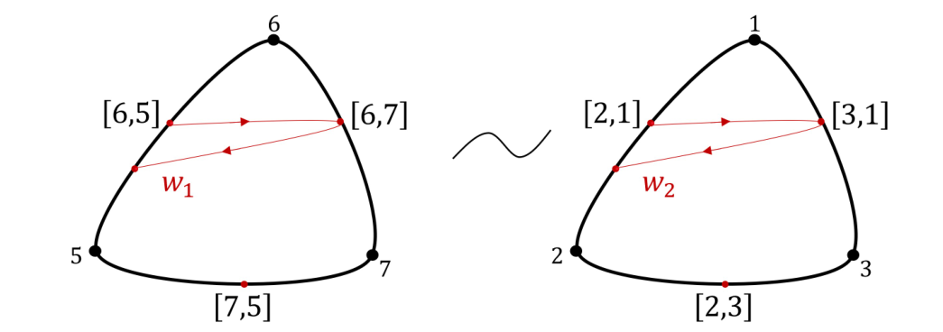
In the case $d=2$ , for $w_{1}=\left[6,5\right]\left[6,7\right]\left[6,5\right]$ and $w_{2}=\left[2,1\right]\left[3,1\right]\left[2,1\right]$ , we have $w_{1}\sim w_{2}$ via any permutation on $\left[n\right]$ satisfying $6\leftrightarrow 1,5\leftrightarrow 2,7\leftrightarrow 3$ (see Figure 4.1).

Furthermore, the support of the word $w=\left[5,6\right]\left[6,7\right]\left[5,6\right]$ $\left[5,8\right]$ is given by $\text{supp}_{0}\left(w\right)=\left\{5,6,7,8\right\}$ and its $2$ -cell support by $\text{supp}_{2}\left(w\right)=\left\{\{5,6,7\},\{6,5,8\}\right\}$ .

Let $B:=\sqrt{n\text{Var}\left(Z\right)}H.$ Since $H$ is symmetric, for every $k\in\mathbb{N}$ ,

$\displaystyle\mathbb{E}[\left\\|H\right\\|_{S_{2k}}^{2k}]$	$\displaystyle=\mathbb{E}\left[\text{Tr}\left(H^{2k}\right)\right]$
	$\displaystyle=\mathbb{E}\left[\text{Tr}\left(\left((n\text{Var}\left(Z\right))^{-1/2}B\right)^{2k}\right)\right]$
	$\displaystyle=\frac{1}{\left(n\text{Var}\left(Z\right)\right)^{k}}\mathbb{E}\left[\text{Tr}\left(B^{2k}\right)\right]$
	$\displaystyle=\frac{1}{\left(n\text{Var}\left(Z\right)\right)^{k}}\sum_{\sigma_{1},\ldots,\sigma_{2k}\in X_{+}^{d-1}}\mathbb{E}\left[B_{\sigma_{1}\sigma_{2}}B_{\sigma_{2}\sigma_{3}}\cdots B_{\sigma_{2k}\sigma_{1}}\right].$	(4.1)

Each term in the sum, $B_{\sigma_{1}\sigma_{2}}B_{\sigma_{2}\sigma_{3}}\cdots B_{\sigma_{2k}\sigma_{1}}$ , can be associated with a string of letters $\sigma_{1}\sigma_{2}\ldots\sigma_{2k}$ . Since $B_{\sigma\sigma^{\prime}}=0$ whenever $\sigma\cup\sigma^{\prime}\notin X^{d}$ , it follows that the list of letters which contribute to the sum in (4.1) are the set of closed words of length $2k+1$ . Using the independent structure of $H$ for different $d-$ cells and the definition of $N_{w}\left(\tau\right)$ we then have

	$\displaystyle\mathbb{E}[\left\\|H\right\\|_{S_{2k}}^{2k}]$	$\displaystyle=\frac{1}{\left(n\text{Var}\left(Z\right)\right)^{k}}\sum_{\tiny\begin{array}[]{c}\text{$w$ a closed word}\\ \text{of length $2k+1$}\end{array}\tiny}\prod_{\tau\in K^{d}}\mathbb{E}\left[B_{\tau}^{N_{w}\left(\tau\right)}\right]$
		$\displaystyle\leq\frac{1}{\left(n\text{Var}\left(Z\right)\right)^{k}}\sum_{\tiny\begin{array}[]{c}\text{$w$ a closed word}\\ \text{of length $2k+1$}\end{array}\tiny}\prod_{\tau\in K^{d}}\left\|\mathbb{E}\left[B_{\tau}^{N_{w}\left(\tau\right)}\right]\right\|,$

where $B_{\tau}:=B_{\sigma\sigma^{\prime}}$ for some $\sigma,\sigma^{\prime}\in X_{+}^{d-1}$ with $\sigma\cup\sigma^{\prime}=\tau$ (observe that the value of $\left|\mathbb{E}\left[B_{\tau}^{N_{w}\left(\tau\right)}\right]\right|$ for any pair $\left(\sigma,\sigma^{\prime}\right)\in X_{+}^{d-1}$ with $\sigma\cup\sigma^{\prime}=\tau$ , is the same, hence the last expression is well defined).

Note that if $N_{w}\left(\tau\right)=1$ , then

\mathbb{E}\left[B_{\tau}^{N_{w}\left(\tau\right)}\right]=\mathbb{E}\left[B_{\tau}\right]=\mathbb{E}\left[Z_{\tau}-\mathbb{E}\left[Z\right]\right]=0,

and hence we only need to address closed words of length $2k+1$ such that

N_{w}\left(\tau\right)\geq 2,\qquad\forall\tau\in\text{supp}_{d}\left(w\right).

(4.2)

Denote by $\mathcal{W}_{2k+1}$ a set of representatives for the equivalence classes of closed words of length $2k+1$ with $N_{w}\left(\tau\right)\geq 2$ for all $\tau\in\text{supp}_{d}\left(w\right)$ . As a consequence of the above remark we obtain

\displaystyle\mathbb{E}\left[\left\|H\right\|_{S_{2k}}^{2k}\right]

\displaystyle\leq\frac{1}{\left(n\text{Var}\left(Z\right)\right)^{k}}\sum_{w\in\mathcal{W}_{2k+1}}\sum_{u\sim w}\prod_{\tau\in\text{supp}_{d}\left(u\right)}\mathbb{E}\left[\left|B_{\tau}\right|^{N_{u}\left(\tau\right)}\right].

For $\tau\in K^{d}$ and $m\in\mathbb{N}$ , define

b_{\tau}^{\left(m\right)}:=\mathbb{E}\left[\left|B_{\tau}\right|^{m}\right],

(4.3)

and note that despite the notation $b_{\tau}^{\left(m\right)}$ is independent of $\tau$ , since all none zero entries of $B$ have the same distribution. Moreover, $\left|\text{supp}_{d}\left(u\right)\right|=\left|\text{supp}_{d}\left(w\right)\right|$ for any two equivalent words $u$ and $w$ . Consequently

	$\displaystyle\mathbb{E}\left[\left\\|H\right\\|_{S_{2k}}^{2k}\right]$	$\displaystyle\leq\frac{1}{\left(n\text{Var}\left(Z\right)\right)^{k}}\sum_{w\in\mathcal{W}_{2k+1}}\sum_{u\sim w}\prod_{\tau\in\text{supp}_{d}\left(w\right)}b_{\tau}^{\left(N_{w}\left(\tau\right)\right)}$
		$\displaystyle=\frac{1}{\left(n\text{Var}\left(Z\right)\right)^{k}}\sum_{w\in\mathcal{W}_{2k+1}}\prod_{\tau\in\text{supp}_{d}\left(w\right)}b_{\tau}^{\left(N_{w}\left(\tau\right)\right)}\left\|\left\{u:u\text{ is a word such that }u\sim w\right\}\right\|,$

Throughout the rest of the argument we work with the following set of representatives: Each equivalence class $[w]$ contains a unique word $u$ with $\mathrm{supp}_{0}(u)=\{1,2,\ldots,|\mathrm{supp_{0}}(u)|\}$ and such that the appearance of the $0$ -cells along the word $u$ , is in increasing order. We choose this word as the unique representative of the equivalence class. Note that given such a representative $u$ for the equivalence class, the remaining elements in the equivalence class are given via a permutation $\mathbf{v}\in[n]^{|\mathrm{supp}_{0}(u)|}$ , taking the word $u$ to the word $\mathbf{v}(u)=\mathbf{v}(u_{1})\mathbf{v}(u_{2})\cdots\mathbf{v}(u_{|\mathrm{supp}_{0}(u)|})$ , where we recall that for a cell $\sigma=[\sigma^{0},\sigma^{1},\ldots,\sigma^{d-1}]$ in $X^{d-1}$ , we define $\mathbf{v}(\sigma)=[\mathbf{v}(\sigma^{0}),\mathbf{v}(\sigma^{1}),\ldots,\mathbf{v}(\sigma^{d-1})]$ . With a slight abuse of notation, we use $\left[n\right]^{m}$ , for $m\in\mathbb{N}$ , to denote all vectors of length $m$ , whose components are distinct and belong to the set $\left[n\right]$ .

Example 4.5.

For $d=2$ and $n=8$ , consider the word $w=\left[5,6\right]\left[6,7\right]\left[5,6\right]$ $\left[6,1\right]\left[1,2\right]$ . The unique representative in the equivalence class of $w$ is $u=[1,2][2,3][1,2][2,4][4,5]$ . Taking the permutation $\mathbf{v}=\left(6,4,8,1,5\right)\in\left[8\right]^{5}$ , gives the equivalent word $\mathbf{v}(u)=[6,4][4,8][6,4][4,1][1,5]$ .

Let $w$ be a representative of an equivalence class. Observe that each closed word $u$ satisfying $u\sim w$ , arises from a unique permutation $\mathbf{v}^{u}\in[n]^{|\mathrm{supp}_{0}(w)|}$ . Hence,

\left|\left\{u:u\text{ a closed word such that }u\sim w\right\}\right|\leq\left|[n]^{|\mathrm{supp}_{0}(w)|}\right|.

Consequently,

$\displaystyle\mathbb{E}\left[\left\\|H\right\\|_{S_{2k}}^{2k}\right]$	$\displaystyle\leq\frac{1}{\left(n\text{Var}\left(Z\right)\right)^{k}}\sum_{w\in\mathcal{W}_{2k+1}}\prod_{\tau\in\text{supp}_{d}\left(w\right)}b_{\tau}^{\left(N_{w}\left(\tau\right)\right)}\left\|[n]^{\|\mathrm{supp}_{0}(w)\|}\right\|$
	$\displaystyle=\frac{1}{\left(n\text{Var}\left(Z\right)\right)^{k}}\sum_{w\in\mathcal{W}_{2k+1}}\sum_{\mathbf{v}\in[n]^{\|\mathrm{supp}_{0}(w)\|}}\prod_{\tau\in\text{supp}_{d}\left(w\right)}b_{\tau}^{\left(N_{w}\left(\tau\right)\right)}$
	$\displaystyle=\frac{1}{\left(n\text{Var}\left(Z\right)\right)^{k}}\sum_{w\in\mathcal{W}_{2k+1}}\sum_{\mathbf{v}\in[n]^{\|\mathrm{supp}_{0}(w)\|}}\prod_{\tau\in\text{supp}_{d}\left(w\right)}b_{\mathbf{v}\left(\tau\right)}^{\left(N_{w}\left(\tau\right)\right)},$	(4.4)

where in the last equality we used the fact that $\left|B_{\mathbf{v}\left(\tau\right)}\right|\overset{\text{law}}{=}\left|B_{\tau}\right|$ , and thus $b_{\tau}^{\left(N_{w}\left(\tau\right)\right)}=b_{\mathbf{v}\left(\tau\right)}^{\left(N_{w}\left(\tau\right)\right)}$ .

Notation 4.6.

Given $G=\left(V_{G},E_{G}\right)\in\mathbb{G}$ we define

S_{d}\left(G\right):=\left\{\tau\in X^{d}\text{ : }\exists\left\{\sigma,\sigma^{\prime}\right\}\in E_{G}\text{ such that $\sigma\cup\sigma^{\prime}=\tau$}\right\},

and

S_{0}\left(G\right)=\left\{i\in\left[n\right]\text{ : }\exists\sigma\in V_{G}\text{ such that $i\in\sigma$}\right\}.

Note that for a word $u$ , $S_{d}\left(G_{u}\right)=\text{supp}_{d}\left(u\right)$ and $S_{0}\left(G_{u}\right)=\text{supp}_{0}\left(u\right)$ .
Denote by $\mathbf{N}_{G}=\left(\mathcal{N}_{G}\left(e\right)\right)_{e\in E_{G}}$ a family of positive weights for the edges in $G$ . For $\tau\in S_{d}\left(G\right)$ define $\mathcal{N}_{G}\left(\tau\right):=\sum_{\underset{\sigma\cup\sigma^{\prime}=\tau}{\left\{\sigma,\sigma^{\prime}\right\}\in E_{G}}}\mathcal{N}_{G}\left(\left\{\sigma,\sigma^{\prime}\right\}\right).$

Notation 4.7.

For a graph $G\in\mathbb{G}$ and weights $\mathbf{N}_{G}=\left(\mathcal{N}_{G}\left(\tau\right)\right)_{\tau\in S_{d}\left(G\right)}$ , denote

\mathcal{G}\left(G;\mathbf{N}_{G}\right)=\sum_{\mathbf{v}\in[n]^{|S_{0}\left(G\right)|}}\prod_{\tau\in S_{d}\left(G\right)}b_{\mathbf{v}\left(\tau\right)}^{\left(\mathcal{N}_{G}\left(\tau\right)\right)}.

Note that $\mathcal{G}\left(G;\mathbf{N}_{G}\right)$ equals $\left|S_{0}\left(G\right)\right|!\cdot{n\choose\left|S_{0}\left(G\right)\right|}\prod_{\tau\in S_{d}\left(G\right)}b_{\tau}^{\left(\mathcal{N}_{G}\left(\tau\right)\right)},$ as $b_{\mathbf{v}\left(\tau\right)}^{\left(\mathcal{N}_{G}\left(\tau\right)\right)}$ does not depend on the choice of $\mathbf{v}$ . Nevertheless, we keep the original notation including the sum in order to apply later on Hölder’s inequality on it.

Using Notations 4.6 and 4.7 , we can write inequality (4.4) as follows

\mathbb{E}\left[\left\|H\right\|_{S_{2k}}^{2k}\right]\leq\frac{1}{\left(n\text{Var}\left(Z\right)\right)^{k}}\sum_{w\in\mathcal{W}_{2k+1}}\mathcal{G}\left(G_{w};\mathbf{N}_{G_{w}}\right),

(4.5)

where the weights $\mathbf{N}_{G_{w}}=\left(N_{w}\left(\tau\right)\right)_{\tau\in\text{supp}_{d}\left(w\right)}$ , are taken to be the crossing numbers.

4.1.1 Reduction to the case of trees

The following result is a generalization of [LVHY18, Lemma 2.9], showing that among all graphs $G\in\mathbb{G}$ , the value $\mathcal{G}\left(G;\mathbf{N}_{G}\right)$ is maximized by trees. This will enable us to restrict attention to trees in the rest of the proof. The main difference is that for $d\geq 2$ , there is more than one way that a cycle in the induced graph can traversed a $d$ -cell (see Figures 4.2, 4.3 and 4.4 ), whereas for $d=1$ such a crossing is unique. In particular, the number of $d-$ cells which are crossed by a cycle of length $\ell$ in $d=1$ is always $\ell$ , while for $d\geq 2$ it is only bounded from above by $\ell$ , and in many cases it is strictly smaller. The analysis corresponding to the only available situation in the graph case, namely Figure 4.4, is similar to that in [LVHY18, Lemma 2.9]. However, new arguments are needed in order to deal with the new cases that does not exist in the one-dimensional case.

Lemma 4.8.

For every word $w\in\mathcal{W}_{2k+1}$ and every family of labelings $\mathbf{N}_{G_{w}}=\left(\mathcal{N}_{G_{w}}\left(e\right)\right)_{e\in E\left(G_{w}\right)}$ for the associated graph $G_{w}$ , there exist a graph $T\in\mathbb{G}$ and labelings $\mathbf{N}_{T}=\left(\mathcal{N}_{T}\left(\tau\right)\right)_{\tau\in S_{d}\left(T\right)}$ (depending on $\mathbf{N}_{G_{w}}$ ), such that the following holds:

1.

$T$ is a tree.
2.

$S_{d}\left(T\right)\subseteq S_{d}\left(G_{w}\right).$
3.

$S_{0}\left(T\right)=S_{0}\left(G_{w}\right)$ .
4.

$\mathcal{N}_{T}\left(\tau\right)\geq\mathcal{N}_{G_{w}}\left(\tau\right),$ $\forall\tau\in S_{d}\left(T\right)$ .
5.

$\sum_{\tau\in S_{d}\left(G_{w}\right)}\mathcal{N}_{G_{w}}\left(\tau\right)=\sum_{\tau\in S_{d}\left(T\right)}\mathcal{N}_{T}\left(\tau\right)$ .
6.

$\mathcal{G}\left(G_{w};\mathbf{N}_{G_{w}}\right)\leq\mathcal{G}\left(T;\mathbf{N}_{T}\right)$ .

Proof.

If $G_{w}$ is a tree, then by setting $T:=G_{w}$ and $\mathcal{N}_{T}\left(\tau\right)=\mathcal{N}_{G_{w}}\left(\tau\right)$ for every $\tau\in S_{d}\left(G\right)$ we are done. Next, assume $G_{w}$ is not a tree, namely it contains a cycle. Denote such a cycle by $e_{1}e_{2}\ldots e_{j}e_{1}$ , where $e_{i}\in E_{G_{w}}$ for all $1\leq i\leq j$ . There are three possible cases:

•

Case $1.1$ : The cycle is contained inside a $d$ -cell. In this case, we define a new graph, induced from $G_{w}$ , by omitting the edge $e_{1}$ , and defining its new labeling via

\mathcal{N}_{\text{new}}(e)=\begin{cases}\mathcal{N}_{G_{w}}(e)&e\notin\{e_{1},e_{j}\}\\ \mathcal{N}_{G_{w}}(e_{1})+\mathcal{N}_{G_{w}}(e_{j})&e=e_{j}\end{cases}.

See Figure 4.2 for an illustration in the case $d=2$ .

•

Case $1.2$ : The cycle is not contained in a $d$ -cell. We observe two possible sub-cases:

–

Case $1.2.1$ : $\exists\tau\in S_{d}\left(G_{w}\right)$ and $\exists i_{1},i_{2}\in\left[j\right]$ distinct such that $e_{i_{1}},e_{i_{2}}$ cross $\tau$ . We define a new graph, induced from $G_{w}$ , by omitting the edge $e_{i_{1}}$ , and defining its new labeling via

\mathcal{N}_{\text{new}}\left(e\right):=\begin{cases}\mathcal{N}_{G_{w}}\left(e\right)&e\notin\left\{e_{i_{1}},e_{i_{2}}\right\}\\ \mathcal{N}_{G_{w}}\left(e_{i_{1}}\right)+\mathcal{N}_{G_{w}}\left(e_{i_{2}}\right)&e=e_{i_{2}}\end{cases},

see Figure 4.3 for an illustration in the case $d=2$ .

–

Case $1.2.2$ : For any $d-$ cell $\tau\in S_{d}\left(G_{w}\right)$ , crossed by the cycle, there exists a unique $i_{\tau}\in\left[j\right]$ , such that $e_{i_{\tau}}$ crosses $\tau$ . Let $\tau_{1},\tau_{2}$ be two distinct $d-$ cells that are both traversed by the cycle (the existence of such cells is guaranteed by the above assumption), with a common $\left(d-1\right)-$ cell. Denote by $e_{i_{\tau_{1}}}$ and $e_{i_{\tau_{2}}}$ , with $i_{\tau_{1}},i_{\tau_{2}}\subset\left[j\right]$ , the unique edges of the cycle, crossing $\tau_{1}$ and $\tau_{2}$ respectively. Then by Jensen’s inequality

	$\displaystyle\mathcal{G}\left(G_{w};\mathbf{N}_{G_{w}}\right)$	$\displaystyle=\sum_{\mathbf{v}\in[n]^{\|S_{0}\left(w\right)\|}}\prod_{i=1}^{2}b_{\mathbf{v}\left(\tau_{i}\right)}^{\left(\mathcal{N}_{G_{w}}\left(\tau_{i}\right)\right)}\prod_{\tau\in S_{d}\left(G_{w}\right)\backslash\left\{\tau_{1},\tau_{2}\right\}}b_{\mathbf{v}\left(\tau\right)}^{\left(\mathcal{N}_{G_{w}}\left(\tau\right)\right)}$
		$\displaystyle\leq\sum_{\mathbf{v}\in[n]^{\|S_{0}\left(w\right)\|}}\prod_{i=1}^{2}\left(b_{\mathbf{v}\left(\tau_{i}\right)}^{\left(\sum_{j=1}^{2}\mathcal{N}_{G_{w}}\left(\tau_{j}\right)\right)}\right)^{\frac{\mathcal{N}_{G_{w}}\left(\tau_{i}\right)}{\sum_{j=1}^{2}\mathcal{N}_{G_{w}}\left(\tau_{j}\right)}}\prod_{\tau\in S_{d}\left(G_{w}\right)\backslash\left\{\tau_{1},\tau_{2}\right\}}b_{\mathbf{v}\left(\tau\right)}^{\left(\mathcal{N}_{G_{w}}\left(\tau\right)\right)}$
		$\displaystyle=\sum_{\mathbf{v}\in[n]^{\|S_{0}\left(w\right)\|}}\prod_{i=1}^{2}\left(b_{\mathbf{v}\left(\tau_{i}\right)}^{\left(\sum_{j=1}^{2}\mathcal{N}_{G_{w}}\left(\tau_{j}\right)\right)}\cdot\prod_{\tau\in S_{d}\left(G_{w}\right)\backslash\left\{\tau_{1},\tau_{2}\right\}}b_{\mathbf{v}\left(\tau\right)}^{\left(\mathcal{N}_{G_{w}}\left(\tau\right)\right)}\right)^{\frac{\mathcal{N}_{G_{w}}\left(\tau_{i}\right)}{\sum_{j=1}^{2}\mathcal{N}_{G_{w}}\left(\tau_{j}\right)}}$

Since $b_{\tau}^{\left(\alpha\right)}=b_{\tau^{\prime}}^{\left(\alpha\right)}$ for all $\tau,\tau^{\prime}\in K^{d}$ , it follows from Hölder’s inequality that

	$\displaystyle\mathcal{G}\left(G_{w};\mathbf{N}_{G_{w}}\right)$	$\displaystyle\leq\prod_{i=1}^{2}\left(\sum_{\mathbf{v}\in[n]^{\|S_{0}\left(w\right)\|}}b_{\mathbf{v}\left(\tau_{i}\right)}^{\left(\sum_{j=1}^{2}\mathcal{N}_{G_{w}}\left(\tau_{j}\right)\right)}\cdot\prod_{\tau\in S_{d}\left(G_{w}\right)\backslash\left\{\tau_{1},\tau_{2}\right\}}b_{\mathbf{v}\left(\tau\right)}^{\left(\mathcal{N}_{G_{w}}\left(\tau\right)\right)}\right)^{\frac{\mathcal{N}_{G_{w}}\left(\tau_{i}\right)}{\sum_{j=1}^{2}\mathcal{N}_{G_{w}}\left(\tau_{j}\right)}}$
		$\displaystyle=\prod_{i=1}^{2}\left(\sum_{\mathbf{v}\in[n]^{\|S_{0}\left(w\right)\|}}b_{\mathbf{v}\left(\tau_{1}\right)}^{\left(\sum_{j=1}^{2}\mathcal{N}_{G_{w}}\left(\tau_{j}\right)\right)}\cdot\prod_{\tau\in S_{d}\left(G_{w}\right)\backslash\left\{\tau_{1},\tau_{2}\right\}}b_{\mathbf{v}\left(\tau\right)}^{\left(\mathcal{N}_{G_{w}}\left(\tau\right)\right)}\right)^{\frac{\mathcal{N}_{G_{w}}\left(\tau_{i}\right)}{\sum_{j=1}^{2}\mathcal{N}_{G_{w}}\left(\tau_{j}\right)}}$
		$\displaystyle=\sum_{\mathbf{v}\in[n]^{\|S_{0}\left(w\right)\|}}b_{\mathbf{v}\left(\tau_{1}\right)}^{\left(\sum_{j=1}^{2}\mathcal{N}_{G_{w}}\left(\tau_{j}\right)\right)}\cdot\prod_{\tau\in S_{d}\left(G_{w}\right)\backslash\left\{\tau_{1},\tau_{2}\right\}}b_{\mathbf{v}\left(\tau\right)}^{\left(\mathcal{N}_{G_{w}}\left(\tau\right)\right)},$

Therefore we can define a new graph $G^{\left(\text{new}\right)}$ by omitting the unique edge which crosses $\tau_{2}$ , namely $e_{i_{\tau_{2}}}$ , and define the graph labelings via

\displaystyle\mathcal{N}_{\text{new}}\left(e\right):=\begin{cases}\mathcal{N}_{G_{w}}\left(e\right)&e\notin\left\{e_{i_{\tau_{1}}},e_{i_{\tau_{2}}}\right\}\\ \mathcal{N}_{G_{w}}\left(e_{i_{\tau_{1}}}\right)+\mathcal{N}_{G_{w}}\left(e_{i_{\tau_{2}}}\right)&e=e_{i_{\tau_{1}}}\end{cases}.

The above computation shows that the new graph together with its new labeling, satisfies all the requirements described in Lemma 4.8. See Figure 4.4 for an illustration in the case $d=2$ .

Note that in all cases, the new graph attained has the same set of vertices as $G_{w}$ , and so $S_{0}\left(G_{w}\right)=S_{0}\left(G^{\left(\text{new}\right)}\right)$ . Moreover, since we merely omit edges which are part of a cycle, the new graph remains connected. Yet, the new graph contains one less cycles than the original graph.

We repeat the above procedure on the graph $G^{\left(\text{new}\right)}$ repeatedly until there are no cycles left. Denote by $T$ a graph attained via this process, and by $\mathbf{N}_{T}:=\left(\mathcal{N}_{T}\left(\tau\right)\right)_{\tau\in S_{d}\left(T\right)}$ the resulting labelings of $S_{d}\left(T\right)$ .

Since $T$ is connected and does not contain any cycle, it is a tree and belongs to $\mathbb{G}$ : denote $V_{T}:=$ $\left\{\sigma_{i}\right\}_{i=1}^{N}$ . Since $T$ is connected, between any $i\neq j$ there is a path, and thus a word which generates it, denoted by $w_{i,j}$ . Assigning all words $w_{1,2}w_{2,3}\ldots w_{N-1,N}$ gives a new word which induces the graph $T$ . Furthermore, it is clear from the construction of $T$ that condition $\left(2\right)-\left(6\right)$ are satisfied, thus concluding the proof. ∎

The following lemma is a generalization of [LVHY18, Lemma 2.10]. As in [LVHY18, Lemma 2.10], we address the leaves of the tree, and use similar ideas in order to apply Hölder’s inequality recursively. The main difference is that for $d=1$ , the authors in [LVHY18, Lemma 2.10] used the following property, which is no longer true for $d\geq 2$ : A crossing of a $1$ -cell is in bijection with the pair of vertices in its boundary. Namely, given a tree $T,$ and a leaf $\sigma=\left\{i\right\}$ , there exists a unique $1-$ cell $\tau=\left\{i,j\right\}$ that contains $i$ and the only possible crossing from $i$ to the remainder of the tree is the cross from $i$ to $j$ . To overcome the new phenomena in the high-dimensional setting, we use additional combinatorial arguments which allow us to complete the argument similarly to [LVHY18, Lemma 2.10].

Lemma 4.9.

For any word $u$ such that $G_{u}$ is a tree and every labelings of its edges $\mathbf{N}_{G_{u}}=\left(\mathcal{N}_{G_{u}}\left(e\right)\right)_{e\in E\left(G_{u}\right)}$ , there exists $S\subseteq S_{d}\left(G_{u}\right)$ and $\left(\mathcal{M}\left(\tau\right)\right)_{\tau\in S}$ such that the following holds:

1.

$\left|S\right|=\left|S_{0}\left(G_{u}\right)\right|-d$ .
2.

$\mathcal{M}\left(\tau\right)\geq\mathcal{N}_{G_{u}}\left(\tau\right)$ for all $\tau\in S$ .
3.

$\sum_{\tau\in S}\mathcal{M}\left(\tau\right)=\sum_{\tau\in S_{d}\left(G_{u}\right)}\mathcal{N}_{G_{u}}\left(\tau\right)$ .

Furthermore, given any $\left(p_{\tau}\right)_{\tau\in S}\subset(0,1]$ such that $\sum_{\tau\in S}\frac{1}{p_{\tau}}=1$

\mathcal{G}\left(G_{u};\mathbf{N}_{G_{u}}\right)\leq d!\prod_{\tau\in S}\left(\sum_{\sigma\in X_{+}^{d-1}}\left(\sum_{i\in\left[n\right],i\notin\sigma}b_{\sigma\omega^{\left(\sigma,i\right)}}^{\left(\mathcal{M}\left(\tau\right)\right)}\right)^{p_{\tau}}\right)^{\frac{1}{p_{\tau}}},

(4.6)

where $\omega^{\left(\sigma,i\right)}\in\Sigma_{\sigma,i}:=\left\{\left.\sigma^{\prime}\in X_{+}^{d-1}\right|i\in\sigma^{\prime}\text{ and $\sigma\overset{K^{d}}{\sim}\sigma^{\prime}$ or $\sigma\overset{K^{d}}{\sim}\overline{\sigma^{\prime}}$}\right\}$ .

Remark.

The expression on the right hand side of (4.6) is independent of the choice of $\omega^{\left(\sigma,i\right)}$ , since $b_{\sigma\sigma^{\prime}}^{\left(\mathcal{M}\left(\tau\right)\right)}=b_{\sigma\sigma^{\prime\prime}}^{\left(\mathcal{M}\left(\tau\right)\right)}$ for any $\sigma^{\prime}$ , $\sigma^{\prime\prime}\in\Sigma_{\sigma,i}$ .

Proof.

The proof proceeds by induction on $\left|S_{0}\left(G_{u}\right)\right|$ . We operate a procedure on the graph $G_{u}$ in order to obtain a new graph which is still a tree, by omitting $0$ -cells from the original graph. This allows us to use the induction hypothesis on the smaller graph. We describe how the omitted $0$ -cell is chosen, and we show there is a 1-1 correspondence between an omitted $0$ -cell and an omitted $d$ -cell. The set $S$ is the set of all omitted $d$ -cells according to this correspondence. We simultaneously prove inequality (4.6), by an additional induction, where in each step we have an omitted $d$ -cell $\tau$ , and we attach to it a number $p_{\tau}\in(0,1]$ . Observe that the set $S$ , which is determined using the mentioned procedure, is independent with the proof of inequality (4.6), and we do it together for the sake of simplicity and coherence.

For the initial case, if $\left|S_{0}\left(G_{u}\right)\right|=d+1,$ then $\left|S_{d}\left(G_{u}\right)\right|=1$ , namely $S_{d}\left(G_{u}\right)=\{\tau_{0}\}$ for some $\tau_{0}\in X^{d}$ , and the result follows readily by setting $S=\{\tau_{0}\}$ and $\mathcal{M}\left(\tau_{0}\right):=\mathcal{N}_{G_{u}}\left(\tau_{0}\right)$ . Indeed, it is clear that conditions $\left(1\right)-\left(3\right)$ are satisfied. Furthermore, given $p_{\tau}>0$ with $\sum_{\tau\in S}\frac{1}{p_{\tau}}=1$ , since $S=\left\{\tau_{0}\right\}$ it follows that $p_{\tau_{0}}=1$ , and therefore

	$\displaystyle\mathcal{G}\left(G_{u};\mathbf{N}_{G_{u}}\right)$	$\displaystyle=\sum_{\mathbf{v}\in[n]^{\|S_{0}\left(G_{u}\right)\|}}\prod_{\tau\in S_{d}\left(G_{u}\right)}b_{\mathbf{v}\left(\tau\right)}^{\left(\mathcal{N}_{G_{u}}\left(\tau\right)\right)}=\sum_{\mathbf{v}\in[n]^{d+1}}b_{\mathbf{v}\left(\tau_{0}\right)}^{\left(\mathcal{M}\left(\tau_{0}\right)\right)}$
		$\displaystyle=\sum_{\mathbf{v}\in[n]^{d}}\sum_{i\in\left[n\right]\backslash\mathbf{v}\left(\sigma_{0}\right)}b_{i\cup\mathbf{v}\left(\sigma_{0}\right)}^{\left(\mathcal{M}\left(\tau_{0}\right)\right)}$
		$\displaystyle\overset{\left(1\right)}{=}d!\sum_{\sigma\in X_{+}^{d-1}}\left(\sum_{i\in\left[n\right],i\notin\sigma}b_{\sigma\omega^{\left(\sigma,i\right)}}^{\left(\mathcal{M}\left(\tau_{0}\right)\right)}\right),$

where $\left(1\right)$ follows because each $\sigma\in X_{+}^{d-1}$ is attained by $d!$ different $\mathbf{v}\in[n]^{d}$ (up to reordering of its entries). This concludes the proof in the case $\left|S_{0}\left(G_{u}\right)\right|=d+1$ .

Let us now describe the induction step. Suppose we have shown that for some $r\in\mathbb{N}$ , whenever $G_{u}$ is a tree with $|S_{0}(G_{u})|>d+r$ , one can find $S=\left\{\tau_{s}\right\}_{s=1}^{r}\subseteq S_{d}\left(G_{u}\right)$ , weights $\left(\mathcal{M}\left(\tau_{s}\right)\right)_{s=1}^{r}$ , a graph $G\in\mathbb{G}$ and weights $\left(\mathcal{N}_{G}\left(\tau\right)\right)_{\tau\in S_{d}\left(G\right)}$ , such that

\displaystyle\mathcal{G}\left(G_{u};\mathbf{N}_{G_{u}}\right)

\displaystyle\leq\prod_{s=1}^{\left|S\right|}\left[\sum_{\mathbf{v}\in[n]^{|S_{0}\left(G\right)|}}\left(\sum_{i\notin\mathbf{v}\left(\sigma_{1}\right)}b_{i\cup\mathbf{v}\left(\sigma_{1}\right)}^{\left(\mathcal{M}\left(\tau_{s}\right)\right)}\right)^{q_{s}}\prod_{\tau\in S_{d}\left(G\right)}b_{\mathbf{v}\left(\tau\right)}^{\left(\mathcal{N}_{G}\left(\tau\right)\right)}\right]^{\frac{1}{\alpha_{s}}},

(4.7)

where

1.
$G$ is a tree with
1. (a)
  
  $\sigma_{1}\in X_{+}^{d-1}$ satisfies $\sigma_{1}\in E\left(G\right)$ .
2. (b)
  
  $S_{d}\left(G\right)\subseteq S_{d}\left(G_{u}\right)$ .
3. (c)
  
  $S_{0}\left(G\right)\subseteq S_{0}\left(G_{u}\right)$ with $\left|S_{0}\left(G\right)\right|=\left|S_{0}\left(G_{u}\right)\right|-r$ .
2.
The weights satisfy
1. (a)
  
  $\mathcal{M}\left(\tau\right)\geq\mathcal{N}_{G_{u}}\left(\tau\right)$ for all $\tau\in S$ .
2. (b)
  
  $\sum_{\tau\in S}\mathcal{M}\left(\tau\right)=\sum_{\tau\in S_{d}\left(G_{u}\right)}\mathcal{N}_{G_{u}}\left(\tau\right)$ .
3. (c)
  
  $\mathcal{N}_{G}\left(\tau\right)\geq\mathcal{N}_{G_{\mathbf{u}}}\left(\tau\right)$ for any $\tau\in S_{d}\left(G\right)$ .
4. (d)
  
  $\sum_{\tau\in S_{d}\left(G_{\mathbf{u}}\right)}\mathcal{N}_{G_{u}}\left(\tau\right)=\sum_{s=1}^{r}\mathcal{M}\left(\tau_{s}\right)+\sum_{\tau\in S_{d}\left(G\right)}\mathcal{N}_{G}\left(\tau\right)$ .
3.
The numbers $q_{s}$ satisfy
1. (a)
  
  $q_{s}=\sum_{j=1}^{r}\frac{p_{\tau_{s}}}{p_{\tau_{j}}}$ for all $1\leq s\leq r$ , where $(p_{\tau})_{\tau\in S}\subset(0,1]$ .
4.

The right-hand side of (4.7) is $1$ -homogeneous in all variables $\left\{b^{\left(\mathcal{N}\left(\tau\right)\right)}\right\}$ which determine the value of $\alpha_{s}$ .

By the induction hypothesis $G$ is a tree and thus must contain a leaf, i.e., vertex of degree one. Denote by $\sigma_{\ell}$ such a leaf and by $\sigma^{\prime}_{\ell}$ the unique $\left(d-1\right)-$ cell such that $\left\{\sigma_{\ell},\sigma^{\prime}_{\ell}\right\}$ is an edge. Set $\tau_{\ell}:=\sigma_{\ell}\cup\sigma^{\prime}_{\ell}$ and let $i_{\ell}\in S_{0}\left(G\right)$ be the unique vertex ( $0-$ cell) in $G$ such that $\tau_{\ell}=\sigma^{\prime}_{\ell}\cup\{i_{\ell}\}$ . Denote by $\hat{\text{$\mathbb{G}$}}$ a subset of $\mathbb{G}$ which contains merely elements from $\mathbb{G}$ which are trees, and

\Psi=\bigcup_{k=1}^{{n\choose d}}\left\{\left(m_{j}\right)_{j\in I};\left|I\right|=k,\text{ $m_{j}$}\in\mathbb{N}\right\},

and define the function $f:\hat{\text{$\mathbb{G}$}}\times\Psi\to\hat{\text{$\mathbb{G}$}}\times\Psi$ (corresponds to a tree $G$ and the labelings of its edges $\left(\mathcal{N}_{G}\left(e\right)\right)_{e\in E\left(G\right)})$ according to the following three possible cases

•

Case $2.1$ : $\tau_{\ell}$ is traversed only by the edge $\left\{\sigma_{\ell},\sigma_{i_{\ell}}\right\}$ and $\left\{\tau\in S_{d}\left(G_{u}\right)|i_{\ell}\in\tau\right\}=\left\{\tau_{\ell}\right\}$ (namely, the $0-$ cell $i_{\ell}$ is contained only in $\tau_{\ell}).$ In this case $f\left(\left(G,\mathbf{N}_{G}\right)\right)=\left(G,\mathbf{N}_{G}\right)$ (namely no changes are done in $G$ and its labelings). See Figure 4.5 for an illustration in the case $d=2$ .

Figure 4.5: A leaf $\sigma_{\ell}$ , in a $2-$ cell $\tau_{\ell}$ , such that $i_{\ell}$ is contained only in the $2-$ cell $\tau_{\ell}$ and $\left\{\sigma_{\ell},\sigma_{i_{\ell}}\right\}$ is the unique edge which crosses $\tau_{\ell}$ .

•

Case $2.2$ : $\tau_{\ell}$ is traversed by an edge, $\left\{\sigma_{j},\sigma_{m}\right\}$ , distinct from $\left\{\sigma_{\ell},\sigma_{i_{\ell}}\right\}$ . In this case $f\left(\left(G,\mathbf{N}_{G}\right)\right)=\left(G_{1},\mathbf{N}_{G_{1}}\right)$ , where $G_{1}$ is the graph obtained from $G$ by omitting the edge $\left\{\sigma_{\ell},\sigma_{i_{\ell}}\right\}$ , and labelings for its edges $\mathbf{N}{}_{G_{1}}=\left(\mathcal{N}_{G_{1}}\left(e\right)\right)_{e\in E\left(G\right)\backslash\left\{\sigma_{\ell},\sigma_{i_{\ell}}\right\}}$ , defined via:

\displaystyle\mathcal{N}_{G_{1}}\left(e\right):=\begin{cases}\mathcal{N}_{G}\left(e\right)&e\notin\left\{\left\{\sigma_{j},\sigma_{m}\right\},\left\{\sigma_{\ell},\sigma_{i_{\ell}}\right\}\right\}\\ \mathcal{N}_{G}\left(\left\{\sigma_{\ell},\sigma_{i_{\ell}}\right\}\right)+\mathcal{N}_{G}\left(\left\{\sigma_{j},\sigma_{m}\right\}\right)&e=\left\{\sigma_{j},\sigma_{m}\right\}\end{cases},

See Figure 4.6 for an illustration in the case $d=2$ .

–

Case $2.3$ : $\tau_{\ell}$ is traversed only by the edge $\left\{\sigma_{\ell},\sigma_{i_{\ell}}\right\}$ , and $i_{\ell}$ is contained in a $d-$ cell, $\tau\in S_{d}\left(G_{u}\right)$ , distinct from $\tau_{\ell}$ . This case guarantees the existence of a $\sigma\in X_{+}^{d-1}$ , such that $\left\{\sigma_{i_{\ell}},\sigma\right\}\in E\left(G_{u}\right)$ and $\sigma_{i_{\ell}}\cup\sigma=\tau^{\prime}\in X^{d}$ , where $\tau^{\prime}\neq\tau_{\ell}$ (otherwise $G$ would have at least two connected components, in contradiction to its connectivity). If there is more then one $\sigma\in X_{+}^{d-1}$ satisfying this condition, we choose one in a deterministic way and define $f\left(\left(G,\mathbf{N}_{G}\right)\right)=\left(G_{2},\mathbf{N}_{G_{2}}\right)$ , where $G_{2}$ is the graph obtained from $G$ by omitting the edge $\left\{\sigma_{\ell},\sigma_{i_{\ell}}\right\}$ , and we equip $G_{2}$ with new labelings for its edges, $\mathbf{N}_{G_{2}}=\left(\mathcal{N}_{G_{2}}\left(e\right)\right)_{e\in E\left(G\right)\backslash\left\{\sigma_{\ell},\sigma_{i_{\ell}}\right\}}$ , defined via:

\displaystyle\mathcal{N}_{G_{2}}\left(e\right):=\begin{cases}\mathcal{N}_{G}\left(e\right)&e\notin\left\{\left\{\sigma,\sigma_{i_{\ell}}\right\},\left\{\sigma_{\ell},\sigma_{i_{\ell}}\right\}\right\}\\ \mathcal{N}_{G}\left(\left\{\sigma_{\ell},\sigma_{i_{\ell}}\right\}\right)+\mathcal{N}_{G}\left(\left\{\sigma,\sigma_{i_{\ell}}\right\}\right)&e=\left\{\sigma,\sigma_{i_{\ell}}\right\}\end{cases},

See Figure 4.7 for illustration in the case $d=2$ .

It is clear that $\mathcal{G}\left(G;\mathbf{N}_{G}\right)=\mathcal{G}\left(G_{1};\mathbf{N}_{G_{1}}\right)$ since $S_{0}\left(G\right)=S_{0}\left(G_{1}\right)$ , $S_{d}\left(G\right)=S_{d}\left(G_{1}\right)$ and the labelings of each $\tau\in S_{d}\left(G\right)$ are the same as those of $G_{1}$ . The inequality $\mathcal{G}\left(G;\mathbf{N}_{G}\right)\leq\mathcal{G}\left(G_{2};\mathbf{N}_{G_{2}}\right)$ follows from the same arguments which were introduced in Lemma (4.8), Case $1.2.2$ . Observe that for $i\in\left\{1,2\right\}$ , $S_{0}\left(G\right)=S_{0}\left(G_{i}\right)$ and $G_{i}$ is itself a tree since it is obtained by omitting a leaf from a tree. Thus $G_{i}\in\mathbb{G}$ for $i\in\left\{1,2,\right\}$ and $f$ is well defined. We may therefore apply $f$ repeatedly. Since $\text{$\left|\mathbb{G}\right|$}<\infty$ , there exists $m_{0}>\ell_{0}\in\mathbb{N}\cup\left\{0\right\}$ for which $f^{m_{0}}\left(\left(G,\mathbf{N}_{G}\right)\right)=f^{\ell_{0}}\left(\left(G,\mathbf{N}_{G}\right)\right)$ . Denote $\left(G_{\text{new}},\mathbf{N}_{G_{\text{new}}}\right):=f^{\ell_{0}}\left(\left(G,\mathbf{N}_{G}\right)\right)\in\mathbb{G}\times\Psi$ , then $f^{m_{0}-\ell_{0}}\left(\left(G_{\text{new}},\mathbf{N}_{G_{\text{new}}}\right)\right)=\left(G_{\text{new}},\mathbf{N}_{G_{\text{new}}}\right)$ which means that $G_{\text{new}}$ is a tree with a leaf as in Case $2.1$ , which we denote again by $\sigma_{\ell}$ . As we have already explained

\mathcal{G}\left(G;\mathbf{N}_{G}\right)\leq\mathcal{G}\left(G_{\text{new}};\mathbf{N}_{G_{\text{new}}}\right),

(4.8)

and $S_{0}\left(G\right)=S_{0}\left(G_{\text{new }}\right)$ . Inequality (4.8) together with the induction hypothesis (4.7) yields the following bound

\displaystyle\mathcal{G}\left(G_{u};\mathbf{N}_{G_{u}}\right)

\displaystyle\leq\prod_{s=1}^{\left|S^{\prime}\right|}\left[\sum_{\mathbf{v}\in[n]^{|S_{0}\left(G_{\text{new}}\right)|}}\left(\sum_{i\notin\mathbf{v}\left(\sigma_{s}\right)}b_{i\cup\mathbf{v}\left(\sigma_{s}\right)}^{\left(\mathcal{M}\left(\tau_{s}\right)\right)}\right)^{q_{s}}\prod_{\tau\in S_{d}\left(G_{\text{new}}\right)}b_{\mathbf{v}\left(\tau\right)}^{\left(\mathcal{N}_{G_{\text{new}}}\left(\tau\right)\right)}\right]^{\frac{1}{\alpha_{s}}},

where $S^{\prime}$ is the set of $d$ -cells removed so far.

We are now turning to bound from above each term in the above multiplication. Fix $1\leq s\leq\left|S^{\prime}\right|$

		$\displaystyle\sum_{\mathbf{v}\in[n]^{\|S_{0}\left(G_{\text{new}}\right)\|}}\left(\sum_{i\notin\mathbf{v}\left(\sigma_{1}\right)}b_{i\cup\mathbf{v}\left(\sigma_{1}\right)}^{\left(\mathcal{M}\left(\tau_{s}\right)\right)}\right)^{q_{s}}\prod_{\tau\in S_{d}\left(G_{\text{new}}\right)}b_{\mathbf{v}\left(\tau\right)}^{\left(\mathcal{N}_{G_{\text{new}}}\left(\tau\right)\right)}$
		$\displaystyle=\sum_{\mathbf{v}\in[n]^{\|S_{0}\left(G_{\text{new}}\right)\|}}\left(\sum_{i\notin\mathbf{v}\left(\sigma_{1}\right)}b_{i\cup\mathbf{v}\left(\sigma_{1}\right)}^{\left(\mathcal{M}\left(\tau_{s}\right)\right)}\right)^{q_{s}}b_{\mathbf{v}\left(\tau_{\ell}\right)}^{\left(\mathcal{N}_{G_{\text{new}}}\left(\tau_{\ell}\right)\right)}\prod_{\tau\in S_{d}\left(G_{\text{new}}\right)\backslash\left\{\tau_{\ell}\right\}}b_{\mathbf{v}\left(\tau\right)}^{\left(\mathcal{N}_{G_{\text{new}}}\left(\tau\right)\right)}$
		$\displaystyle\overset{\left(1\right)}{=}\sum_{\mathbf{v}\in[n]^{\|S_{0}\left(G_{\text{new}}\right)\|}}\left(\sum_{i\notin\mathbf{v}\left(\sigma_{i_{\ell}}\right)}b_{i\cup\mathbf{v}\left(\sigma_{i_{\ell}}\right)}^{\left(\mathcal{M}\left(\tau_{s}\right)\right)}\right)^{q_{s}}b_{\mathbf{v}\left(\tau_{\ell}\right)}^{\left(\mathcal{N}_{G_{\text{new}}}\left(\tau_{\ell}\right)\right)}\prod_{\tau\in S_{d}\left(G_{\text{new}}\right)\backslash\left\{\tau_{\ell}\right\}}b_{\mathbf{v}\left(\tau\right)}^{\left(\mathcal{N}_{G_{\text{new}}}\left(\tau\right)\right)},$		(4.9)

where $\left(1\right)$ follows since $b_{\tau}^{\left(\mathcal{M}\left(\tau_{s}\right)\right)}$ does not depend on the $d$ -cell $\tau$ .

We define a new graph induced from $G_{\text{new}}$ , denoted as $G^{\prime}$ , by omitting the $0-$ cell $i_{\ell}$ . Thus $S_{0}\left(G^{\prime}\right)=S_{0}\left(G_{\text{new}}\right)\backslash\left\{i_{\ell}\right\}$ and $S_{d}\left(G^{\prime}\right)=S_{d}\left(G_{\text{new}}\right)\backslash\left\{\tau_{\ell}\right\}.$ Moreover, for any $\tau\in S_{d}\left(G^{\prime}\right)$ , define

\mathcal{N}_{G^{\prime}}\left(\tau\right):=\mathcal{N}_{G_{\text{new}}}\left(\tau\right).

(4.10)

For any $n\geq m>d$

	$\displaystyle\left\|\left[n\right]^{m}\right\|$	$\displaystyle=\frac{n!}{\left(n-m\right)!}=\left(n-m+1\right)\frac{n!}{\left(n-m+1\right)!}=\left(n-m+1\right)\left\|\left[n\right]^{m-1}\right\|$
		$\displaystyle<\left(n-d\right)\left\|\left[n\right]^{m-1}\right\|.$		(4.11)

By the induction hypothesis $\left|S_{0}\left(G_{\text{new}}\right)\right|=\left|S_{0}\left(G\right)\right|\geq d+1$ and $\left|S_{0}\left(G^{\prime}\right)\right|=\left|S_{0}\left(G_{\text{new}}\right)\right|-1$ , thus we may conclude from (4.11) and (4.9) that $\mathcal{G}\left(G_{u};\mathbf{N}_{G_{u}}\right)$ is bounded from above by

\sum_{\mathbf{v}\in[n]^{|S_{0}\left(G^{\prime}\right)|}}\left(\sum_{i\notin\mathbf{v}\left(\sigma_{i_{\ell}}\right)}b_{i\cup\mathbf{v}\left(\sigma_{i_{\ell}}\right)}^{\left(\mathcal{M}\left(\tau_{s}\right)\right)}\right)^{q_{s}}\left(\sum_{i\notin\mathbf{v}\left(\sigma_{i_{\ell}}\right)}b_{i\cup\mathbf{v}\left(\sigma_{i_{\ell}}\right)}^{\left(\mathcal{N}_{G_{\text{new}}}\left(\tau_{\ell}\right)\right)}\right)\prod_{\tau\in S_{d}\left(G^{\prime}\right)}b_{\mathbf{v}\left(\tau\right)}^{\left(\mathcal{N}_{G^{\prime}}\left(\tau\right)\right)},

(4.12)

where $\mathbf{v}\left(\sigma_{i_{\ell}}\right)$ is well defined since $i_{\ell}\notin\sigma_{i_{\ell}}\subseteq S_{0}\left(G^{\prime}\right)$ . Since,

(4.12)

\displaystyle=\sum_{\mathbf{v}\in[n]^{|S_{0}\left(G\right)|}}\Bigg(\Bigg(\sum_{i\notin\mathbf{v}\left(\sigma_{i_{\ell}}\right)}b_{i\cup\mathbf{v}\left(\sigma_{i_{\ell}}\right)}^{{}_{\left(\mathcal{M}\left(\tau_{s}\right)\right)}}\Bigg)^{q^{\prime}_{s}}\!\!\!\prod_{\tau\in S_{d}\left(G^{\prime}\right)}b_{\mathbf{v}\left(\tau\right)}^{{}_{\left(\mathcal{N}_{G^{\prime}}\left(\tau\right)\right)}}\Bigg)^{\frac{q_{s}}{q^{\prime}_{s}}}\Bigg(\Bigg(\sum_{i\notin\mathbf{v}\left(\sigma_{i_{\ell}}\right)}b_{i\cup\mathbf{v}\left(\sigma_{i_{\ell}}\right)}^{{}_{\left(\mathcal{N}_{G_{\text{new}}}\left(\tau_{\ell}\right)\right)}}\Bigg)^{q_{\ell}}\!\!\!\prod_{\tau\in S_{d}\left(G^{\prime}\right)}b_{\mathbf{v}\left(\tau\right)}^{{}_{\left(\mathcal{N}_{G^{\prime}}\left(\tau\right)\right)}}\Bigg)^{\frac{1}{q_{\ell}}},

where $q^{\prime}_{s}=\sum_{\tau\in S^{\prime}\cup\left\{\tau_{\ell}\right\}}\frac{p_{\tau_{s}}}{p_{\tau}}$ , $q_{\ell}=\sum_{\tau\in S^{\prime}\cup\left\{\tau_{\ell}\right\}}\frac{p_{\tau_{\ell}}}{p_{\tau}}$ , and one can readily verify that $\frac{q_{s}}{q^{\prime}_{s}}+\frac{1}{q_{\ell}}=1$ ,it follows from Hölder’s inequality that (4.12) is bounded from above by

\displaystyle\Bigg[\sum_{{}_{\mathbf{v}\in[n]^{|S_{0}\left(G\right)|}}}\Bigg(\sum_{{}_{i\notin\mathbf{v}\left(\sigma_{i_{\ell}}\right)}}b_{i\cup\mathbf{v}\left(\sigma_{i_{\ell}}\right)}^{{}_{\left(\mathcal{M}\left(\tau_{s}\right)\right)}}\Bigg)^{q^{\prime}_{s}}\!\!\!\prod_{{}_{\tau\in S_{d}\left(G^{\prime}\right)}}\!\!b_{\mathbf{v}\left(\tau\right)}^{{}_{\left(\mathcal{N}_{G^{\prime}}\left(\tau\right)\right)}}\Bigg]^{\frac{q_{s}}{q^{\prime}_{s}}}\Bigg[\Bigg(\sum_{{}_{\mathbf{v}\in[n]^{|S_{0}\left(G\right)|}}}\Bigg(\sum_{{}_{i\notin\mathbf{v}\left(\sigma_{i_{\ell}}\right)}}b_{i\cup\mathbf{v}\left(\sigma_{i_{\ell}}\right)}^{{}_{\left(\mathcal{N}_{G_{\text{new}}}\left(\tau_{\ell}\right)\right)}}\Bigg)^{q_{\ell}}\!\!\!\prod_{{}_{\tau\in S_{d}\left(G^{\prime}\right)}}\!\!b_{\mathbf{v}\left(\tau\right)}^{{}_{\left(\mathcal{N}_{G^{\prime}}\left(\tau\right)\right)}}\Bigg)\Bigg]^{\frac{1}{q_{\ell}}},

(4.13)

with the same degree of homogeneity in each variable $\left\{b^{\left(\mathcal{N}\left(\tau\right)\right)}\right\}$ as of those in term (4.12).

Denoting $\tau_{r+1}:=\tau_{\ell}$ and $S=S^{\prime}\cup\left\{\tau_{r+1}\right\}$ , and replacing every term in the induction hypothesis (4.7) by the upper bound in (4.13), gives

\mathcal{G}\left(G_{u};\mathbf{N}_{G_{u}}\right)\leq\prod_{s=1}^{\left|S\right|}\left[\sum_{\mathbf{v}\in[n]^{|S_{0}\left(G^{\prime}\right)|}}\left(\sum_{i\notin\mathbf{v}\left(\sigma_{i_{\ell}}\right)}b_{i\cup\mathbf{v}\left(\sigma_{i_{\ell}}\right)}^{\left(\mathcal{M}\left(\tau_{s}\right)\right)}\right)^{\widehat{q_{s}}}\prod_{\tau\in S_{d}\left(G^{\prime}\right)}b_{\mathbf{v}\left(\tau\right)}^{\left(\mathcal{N}_{G^{\prime}}\left(\tau\right)\right)}\right]^{\frac{1}{\widehat{\alpha_{s}}}},

(4.14)

where

\widehat{q_{s}}:=\begin{cases}q^{\prime}_{s}&\text{for $1\leq s\leq r$}\\ q_{\ell}&\text{for $s=r+1$}\end{cases},\qquad\mathcal{M}\left(\tau_{s}\right):=\begin{cases}\mathcal{M}\left(\tau_{s}\right)&\text{for $1\leq s\leq r$}\\ \mathcal{N}_{G_{\text{new}}}\left(\tau_{\ell}\right)&\text{for $s=r+1$}\end{cases},\qquad\widehat{\alpha_{s}}:=\begin{cases}\frac{\alpha_{s}q^{\prime}_{s}}{q_{s}}&\text{for $1\leq s\leq r$}\\ \frac{q_{\ell}}{\sum_{j=1}^{r}\frac{1}{\alpha_{s}}}&\text{for $s=r+1$}\end{cases}.

Following the above construction, it is clear that all conditions besides 2(d) are satisfied by the relative parameters in (4.14), where for 2(d) we observe that by the induction hypothesis

	$\displaystyle\sum_{\tau\in S_{d}\left(G_{\mathbf{u}}\right)}\mathcal{N}_{G_{\mathbf{u}}}\left(\tau\right)$	$\displaystyle=\sum_{s=1}^{r}\mathcal{M}\left(\tau_{s}\right)+\sum_{\tau\in S_{d}\left(G\right)}\mathcal{N}_{G}\left(\tau\right)$
		$\displaystyle\overset{\left(1\right)}{=}\sum_{s=1}^{r}\mathcal{M}\left(\tau_{s}\right)+\sum_{\tau\in S_{d}\left(G_{\text{new}}\right)}\mathcal{N}_{G_{\text{new}}}\left(\tau\right)$
		$\displaystyle=\sum_{s=1}^{r}\mathcal{M}\left(\tau_{s}\right)+\mathcal{N}_{G_{\text{new}}}\left(\tau_{\ell}\right)+\sum_{\tau\in S_{d}\left(G_{\text{new}}\right)\backslash\left\{\tau_{\ell}\right\}}\mathcal{N}_{G_{\text{new}}}\left(\tau\right)$
		$\displaystyle\overset{\left(2\right)}{=}\sum_{s=1}^{r+1}\mathcal{M}\left(\tau_{s}\right)+\sum_{\tau\in S_{d}\left(G^{\prime}\right)}\mathcal{N}_{G^{\prime}}\left(\tau\right),$

where $\left(1\right)$ follows by the construction of $G_{\text{new}}$ using the function $f$ and $\left(2\right)$ follows from our definition in (4.10). This proves the induction step, $r\to r+1$ .

The above induction guarantees the validity of the induction hypothesis for $r=\left|S_{0}\left(G_{u}\right)\right|-d$ , that is, we have proved the following bound

\displaystyle\mathcal{G}\left(G_{u};\mathbf{N}_{G_{u}}\right)\leq\prod_{s=1}^{\left|S\right|}\left[\sum_{\mathbf{v}\in[n]^{d}}\left(\sum_{i\notin\mathbf{v}\left(\sigma_{0}\right)}b_{i\cup\mathbf{v}\left(\sigma_{0}\right)}^{\left(\mathcal{M}\left(\tau_{s}\right)\right)}\right)^{\sum_{\tau\in S_{G_{u}}}\frac{p_{\tau_{s}}}{p_{\tau}}}\right]^{\frac{1}{\alpha_{s}}},

where $\sigma_{0}=\left[1,2,\ldots,d\right]\in X_{\pm}^{d-1}$ and $S\subseteq S_{d}\left(G_{u}\right)$ with $\left|S\right|=\left|S_{0}\left(G_{u}\right)\right|-d$ is the set of $d$ -cells removed in the process. Recall that we assume $\sum_{\tau\in S}\frac{1}{p_{\tau}}=1$ , hence we conclude that $\mathcal{G}\left(G_{u};\mathbf{N}_{G_{u}}\right)$ is bounded from above by

\prod_{s=1}^{\left|S\right|}\left[\sum_{\mathbf{v}\in[n]^{d}}\left(\sum_{i\notin\mathbf{v}\left(\sigma_{0}\right)}b_{i\cup\mathbf{v}\left(\sigma_{0}\right)}^{\left(\mathcal{M}\left(\tau_{s}\right)\right)}\right)^{p_{\tau_{s}}}\right]^{\frac{1}{\alpha_{s}}}.

(4.15)

The induction argument guarantees that the term in equation (4.15) is $1$ -homogeneous in all variables $b^{\left(\mathcal{M}\left(\tau_{s}\right)\right)}$ . It must therefore necessarily be the case that $\alpha_{s}=p_{\tau_{s}}$ . Consequently

	$\displaystyle\mathcal{G}\left(G_{u};\mathbf{N}_{G_{u}}\right)$	$\displaystyle\leq\prod_{s=1}^{\left\|S\right\|}\left[\sum_{\mathbf{v}\in[n]^{d}}\left(\sum_{i\notin\mathbf{v}\left(\sigma_{0}\right)}b_{i\cup\mathbf{v}\left(\sigma_{0}\right)}^{\left(\mathcal{M}\left(\tau_{s}\right)\right)}\right)^{p_{\tau_{s}}}\right]^{\frac{1}{p_{\tau_{s}}}}$
		$\displaystyle\overset{\left(1\right)}{=}\prod_{\tau\in S}\left[d!\sum_{\sigma\in X_{+}^{d-1}}\left(\sum_{i\in\left[n\right],i\notin\sigma}b_{\sigma\omega^{\left(\sigma,i\right)}}^{\left(\mathcal{M}\left(\tau\right)\right)}\right)^{p_{\tau}}\right]^{\frac{1}{p_{\tau}}}$
		$\displaystyle\overset{\left(2\right)}{=}d!\prod_{\tau\in S}\left[\sum_{\sigma\in X_{+}^{d-1}}\left(\sum_{i\in\left[n\right],i\notin\sigma}b_{\sigma\omega^{\left(\sigma,i\right)}}^{\left(\mathcal{M}\left(\tau\right)\right)}\right)^{p_{\tau}}\right]^{\frac{1}{p_{\tau}}},$

where $\omega^{\left(\sigma,i\right)}\in\Sigma_{\sigma,i}$ , $\left(1\right)$ follows from the same arguments which were stated in the initial step and $\left(2\right)$ follows because $\sum_{\tau\in S}\frac{1}{p_{\tau}}=1$ . This concludes the proof of Lemma 4.9.

∎

4.1.2 Back to the proof of Theorem 2.1

Let $w\in\mathcal{W}_{2k+1}$ and $\mathbf{N}_{G_{w}}=\left(N_{w}\left(e\right)\right)_{e\in E_{w}}$ . This choice of labeling implies that $\mathcal{N}_{G_{w}}\left(\tau\right)=N_{w}\left(\tau\right)$ for all $\tau\in\text{supp}_{d}\left(w\right).$ Let $T$ be the graph obtained from Lemma 4.8, and apply Lemma 4.9 to it and its labeling $\left(\mathcal{N}_{T}\left(\tau\right)\right)_{\tau\in S_{d}\left(T\right)}$ , using $p_{\tau}=\frac{2k}{\mathcal{M}\left(\tau\right)}$ for $\tau\in S$ , where $\left(\mathcal{M}\left(\tau\right)\right)_{\tau\in S}$ is the vector from Lemma 4.9. Note that this is a valid choice for $\left(p_{\tau}\right)_{\tau\in S}$ since:

\displaystyle\sum_{\tau\in S_{T}}\frac{1}{p_{\tau}}

\displaystyle=\frac{\sum_{\tau\in S}\mathcal{M}\left(\tau\right)}{2k}\overset{{}_{(1)}}{=}\frac{\sum_{\tau\in S_{d}\left(T\right)}\mathcal{N}_{T}\left(\tau\right)}{2k}\overset{{}_{(2)}}{=}\frac{\sum_{\tau\in S_{d}\left(G_{w}\right)}\mathcal{N}_{G_{w}}\left(\tau\right)}{2k}=\frac{\sum_{\tau\in S_{d}\left(G_{w}\right)}N_{w}\left(\tau\right)}{2k}\overset{{}_{(3)}}{=}\frac{2k}{2k}=1,

where $(1)$ follows from Lemma 4.9, $(2)$ follows from Lemma 4.8, $(3)$ follows since $w\in\mathcal{W}_{2k+1}$ .

Hence, by Lemma 4.9

\mathcal{G}\left(T;\mathbf{N}_{T}\right)\leq d!\cdot\prod_{\tau\in S}\left[\sum_{\sigma\in X_{+}^{d-1}}\left(\sum_{i\in\left[n\right],i\notin\sigma}b_{\sigma\omega^{\left(\sigma,i\right)}}^{\left(\mathcal{M}\left(\tau\right)\right)}\right)^{\frac{2k}{\mathcal{M}\left(\tau\right)}}\right]^{\frac{\mathcal{M}\left(\tau\right)}{2k}}.

(4.16)

Recall that for $k\in\mathbb{N}$ , we defined

\theta_{k}:=\sqrt{\frac{n-d}{n}}{n\choose d}^{\frac{1}{2k}}\qquad,\qquad\theta_{k}^{*}:=\left\|Z_{\tau}-\mathbb{E}\left[Z\right]\right\|_{\infty}\left({n\choose d}\cdot\frac{d\left(n-d\right)}{\left(n\text{Var}\left(Z\right)\right)^{k}}\right)^{\frac{1}{2k}},

which one can verify equal to

\theta_{k}:=\left(\sum_{\sigma\in X_{+}^{d-1}}\left(\sum_{i\in\left[n\right],i\notin\sigma}\mathbb{E}\left[\left|H_{\sigma\omega^{\left(\sigma,i\right)}}\right|^{2}\right]\right)^{k}\right)^{\frac{1}{2k}}\qquad\text{and}\qquad\text{ }\theta_{k}^{*}:=\left(\sum_{\sigma,\sigma^{\prime}\in X_{+}^{d-1}}\left\|H_{\sigma\sigma^{\prime}}\right\|_{\infty}^{2k}\right)^{\frac{1}{2k}},

where $\omega^{\left(i\right)}\in\Sigma_{\sigma,i}$ is arbitrary. Observe the product term on (4.16) and note that

\displaystyle\sum_{\sigma\in X_{+}^{d-1}}\left(\sum_{i\in\left[n\right],i\notin\sigma}b_{\sigma\omega^{\left(\sigma,i\right)}}^{\left(\mathcal{M}\left(\tau\right)\right)}\right)^{\frac{2k}{\mathcal{M}\left(\tau\right)}}

\displaystyle=\sum_{\sigma\in X_{+}^{d-1}}\left(\sum_{i\in\left[n\right],i\notin\sigma}\mathbb{E}\left[\left|B_{\sigma\omega^{\left(\sigma,i\right)}}\right|^{\mathcal{M}\left(\tau\right)}\right]\right)^{\frac{2k}{\mathcal{M}\left(\tau\right)}}.

(4.17)

Since Lemma 4.9, Lemma 4.8 and the choice of $\mathbf{N}_{G_{w}}$ together with (4.2) implies

\displaystyle\mathcal{M}\left(\tau\right)\geq\mathcal{N}_{T}\left(\tau\right)\geq\mathcal{N}_{G_{w}}\left(\tau\right)=N_{w}\left(\tau\right)\geq 2,

it follows that

	LHS of (4.17)	$\displaystyle=\sum_{\sigma\in X_{+}^{d-1}}\left(\sum_{i\in\left[n\right],i\notin\sigma}\mathbb{E}\left[\left\|B_{\sigma\omega^{\left(\sigma,i\right)}}\right\|^{2}\left\|B_{\sigma\omega^{\left(\sigma,i\right)}}\right\|^{\mathcal{M}\left(\tau\right)-2}\right]\right)^{\frac{2k}{\mathcal{M}\left(\tau\right)}}$
		$\displaystyle\leq\sum_{\sigma\in X_{+}^{d-1}}\left[\left(\sum_{i\in\left[n\right],i\notin\sigma}\mathbb{E}\left[\left\|B_{\sigma\omega^{\left(\sigma,i\right)}}\right\|^{2}\right]\right)^{\frac{2k}{\mathcal{M}\left(\tau\right)}}\cdot\max_{\sigma^{\prime}\in X_{+}^{d-1}}\left\\|B_{\sigma\sigma^{\prime}}\right\\|_{\infty}^{\frac{2k\left(\mathcal{M}\left(\tau\right)-2\right)}{\mathcal{M}\left(\tau\right)}}\right].$

Applying Hölder’s inequality with $\frac{2}{\mathcal{M}\left(\tau\right)}+\frac{\mathcal{M}\left(\tau\right)-2}{\mathcal{M}\left(\tau\right)}=1$ , the last expression is bounded from above by

		$\displaystyle\left(\sum_{\sigma\in X_{+}^{d-1}}\left(\sum_{i\in\left[n\right],i\notin\sigma}\mathbb{E}\left[\left\|B_{\sigma\omega^{\left(\sigma,i\right)}}\right\|^{2}\right]\right)^{k}\right)^{\frac{2}{\mathcal{M}\left(\tau\right)}}\cdot\left(\sum_{\sigma\in X_{+}^{d-1}}\max_{\sigma^{\prime}\in X_{+}^{d-1}}\left\\|B_{\sigma\sigma^{\prime}}\right\\|_{\infty}^{2k}\right)^{\frac{\mathcal{M}\left(\tau\right)-2}{\mathcal{M}\left(\tau\right)}}$
		$\displaystyle\leq\left(\sum_{\sigma\in X_{+}^{d-1}}\left(\sum_{i\in\left[n\right],i\notin\sigma}\mathbb{E}\left[\left\|B_{\sigma\omega^{\left(\sigma,i\right)}}\right\|^{2}\right]\right)^{k}\right)^{\frac{2}{\mathcal{M}\left(\tau\right)}}\cdot\left(\sum_{\sigma,\sigma^{\prime}\in X_{+}^{d-1}}\left\\|B_{\sigma\sigma^{\prime}}\right\\|_{\infty}^{2k}\right)^{\frac{\mathcal{M}\left(\tau\right)-2}{\mathcal{M}\left(\tau\right)}}$
		$\displaystyle=\left(n\text{Var}\left(Z\right)\right)^{k}\theta_{k}^{\frac{4k}{\mathcal{M}\left(\tau\right)}}\cdot\left(\theta_{k}^{*}\right)^{\frac{2k\left(\mathcal{M}\left(\tau\right)-2\right)}{\mathcal{M}\left(\tau\right)}}.$

Combining all of the above gives

	$\displaystyle\mathcal{G}\left(T;\mathbf{N}_{T}\right)$	$\displaystyle\leq d!\cdot\prod_{\tau\in S}\left[\left(n\text{Var}\left(Z\right)\right)^{k}\theta_{k}^{\frac{4k}{\mathcal{M}\left(\tau\right)}}\cdot\left(\theta_{k}^{*}\right)^{\frac{2k\left(\mathcal{M}\left(\tau\right)-2\right)}{\mathcal{M}\left(\tau\right)}}\right]^{\frac{\mathcal{M}\left(\tau\right)}{2k}}$
		$\displaystyle=d!\cdot\left(n\text{Var}\left(Z\right)\right)^{\frac{\sum_{\tau\in S}\mathcal{M}\left(\tau\right)}{2}}\theta_{k}^{2\left\|S\right\|}\cdot\left(\theta_{k}^{*}\right)^{\left(\sum_{\tau\in S}\mathcal{M}\left(\tau\right)\right)-2\left\|S\right\|}.$		(4.18)

We turn to estimate the powers in (4.18). Using once more Lemma 4.9, Lemma 4.8, the choice of $\mathbf{N}_{G_{w}}$ and that $w\in\mathcal{W}_{2k+1}$ gives

\displaystyle\sum_{\tau\in S}\mathcal{M}\left(\tau\right)

\displaystyle=\sum_{\tau\in S_{d}\left(T\right)}\mathcal{N}_{T}\left(\tau\right)=\sum_{\tau\in S_{d}\left(G_{w}\right)}\mathcal{N}_{G_{w}}\left(\tau\right)=\sum_{\tau\in\text{supp}_{d}\left(w\right)}N_{w}\left(\tau\right)=2k

and

\left|S\right|=\left|S_{0}\left(T\right)\right|-d=\left|S_{0}\left(G_{w}\right)\right|-d.

Hence, by Lemma 4.8

\mathcal{G}\left(G_{w};\mathbf{N}_{G_{w}}\right)\leq\mathcal{G}\left(T;\mathbf{N}_{T}\right)\leq d!\cdot\left(n\text{Var}\left(Z\right)\right)^{k}\cdot\theta_{k}^{2\left(\left|S_{0}\left(G_{w}\right)\right|-d\right)}\cdot\left(\theta_{k}^{*}\right)^{2k-2\left(\left|S_{0}\left(G_{w}\right)\right|-d\right)}.

Using (4.5), we conclude

\displaystyle\mathbb{E}\left[\left\|H\right\|_{S_{2k}}^{2k}\right]

\displaystyle\leq d!\cdot\sum_{w\in\mathcal{W}_{2k+1}}\theta_{k}^{2\left(\left|S_{0}\left(G_{w}\right)\right|-d\right)}\cdot\left(\theta_{k}^{*}\right)^{2k-2\left(\left|S_{0}\left(G_{w}\right)\right|-d\right)}.

By rescaling the matrix $H$ , we may assume without loss of generality that $\theta_{k}^{*}=1$ . Consequently,

\displaystyle\mathbb{E}\left[\left\|H\right\|_{S_{2k}}^{2k}\right]

\displaystyle\leq d!\sum_{w\in\mathcal{W}_{2k+1}}\theta_{k}^{2\left(\left|S_{0}\left(G_{w}\right)\right|-d\right)}=d!\sum_{w\in\mathcal{W}_{2k+1}}\theta_{k}^{2\left(\left|\text{supp}_{0}\left(w\right)\right|-d\right)}

(4.19)

We will now show that the right hand side of (4.19) is bounded from above by a function depending on $\mathbb{E}\left[\left\|Y\right\|_{S_{2k}}^{2k}\right]$ , where $Y$ is the matrix from Section 3 with $p_{0}=\frac{1}{4}$ . As we have already shown

$\displaystyle\mathbb{E}\left[\left\\|Y\right\\|_{S_{2k}}^{2k}\right]$	$\displaystyle=\sum_{w\in\mathcal{W}_{2k+1}}\sum_{u\sim w}\prod_{\tau\in\text{supp}_{d}\left(u\right)}\mathbb{E}\left[Y_{\tau}^{N_{u}\left(\tau\right)}\right]$
	$\displaystyle\overset{\left(1\right)}{\geq}\sum_{w\in\mathcal{W}_{2k+1}}\sum_{u\sim w}1$
	$\displaystyle=\sum_{w\in\mathcal{W}_{2k+1}}\#\left\{u\text{ ; $u$ is a word with $u\sim w$}\right\},$	(4.20)

where $\left(1\right)$ follows since $\mathbb{E}\left[Y_{\tau}^{m}\right]\geq 1$ for all $m\geq 2$ , and $\mathbb{E}\left[Y_{\tau}^{m}\right]=0$ for $m=1$ . We turn to estimate the sum in (4.20) showing that

\#\left\{u\text{ a word ; $u\sim w$}\right\}\geq\frac{\left(r-d+1\right)!}{\left(r-\left|\text{supp}_{0}\left(w\right)\right|\right)!}.

Indeed, fix $w\in\mathcal{W}_{2k+1}$ , with $w=\sigma_{1}\cdots\sigma_{2k}\sigma_{1}$ , and $\sigma_{1}=\left[\sigma_{1}^{0},\ldots,\sigma_{1}^{d-1}\right]$ . Define a set of permutations on $\left[r\right]$ , denoted $\Psi$ , for which each permutation $\pi$ fixes $\left(\sigma_{1}^{i}\right)_{i=1}^{d-1}$ , takes $\sigma_{1}^{0}$ to some number in the set $\left[r\right]\backslash\left\{\sigma_{1}^{j}\right\}_{j=1}^{d-1}$ , and each new appearance of $0-$ cell, takes to some number in $\left[r\right]$ which did not appear earlier. Each permutation in the above set, induces a new word which is equivalent to $w$ . Observe that each choice on the image of $\sigma_{1}^{0}$ defines a different word, since the image of $\sigma_{1}$ would be different (because $\left(\sigma_{1}^{i}\right)_{i=1}^{d-1}$ are fixed). Consequently,

\#\left\{u\text{ a word ; $u\sim w$}\right\}\geq\left|\Psi\right|=\left(r-\left(d-1\right)\right)\left(r-d\right)\cdots\left(r-\left(\text{supp}_{0}\left(w\right)-1\right)\right)=\frac{\left(r-d+1\right)!}{\left(r-\left|\text{supp}_{0}\left(w\right)\right|\right)!}.

Using the above estimation in (4.20) gives

\mathbb{E}\left[\left\|Y\right\|_{S_{2k}}^{2k}\right]\geq\sum_{w\in\mathcal{W}_{2k+1}}\frac{\left(r-d+1\right)!}{\left(r-\left|\text{supp}_{0}\left(w\right)\right|\right)!}.

(4.21)

From (4.2) we know that $\left|\text{supp}_{d}\left(w\right)\right|<k+1$ and since $\left|\text{supp}_{0}\left(w\right)\right|\leq\left|\text{supp}_{d}\left(w\right)\right|+d$ , we obtain $\left|\text{supp}_{0}\left(w\right)\right|<k+d+1.$ Set $r=\left[\theta_{k}^{2}\right]+k+d+1$ . For $\ell_{0}:=r-d+1$ and $m_{0}:=\left|\text{supp}_{0}\left(w\right)\right|-d+1$ , we observe that $\left|\text{supp}_{0}\left(w\right)\right|<k+d+1\leq r$ implies $m_{0}<\ell_{0}$ . As $\frac{\left(\ell-1\right)!}{\left(\ell-m\right)!}\geq\left(\ell-m+1\right)^{m-1}$ for any $\ell\geq m$ and thus

	$\displaystyle\frac{\left(r-d\right)!}{\left(r-\left\|\text{supp}_{0}\left(w\right)\right\|\right)!}$	$\displaystyle\geq\left(r-\left\|\text{supp}_{0}\left(w\right)\right\|+1\right)^{\left\|\text{supp}_{0}\left(w\right)\right\|-d}$
		$\displaystyle=\left(\left[\theta_{k}^{2}\right]+k+d+1-\left\|\text{supp}_{0}\left(w\right)\right\|+1\right)^{\left\|\text{supp}_{0}\left(w\right)\right\|-d}$
		$\displaystyle\geq\left(\left[\theta_{k}^{2}\right]+1\right)^{\left\|\text{supp}_{0}\left(w\right)\right\|-d}$
		$\displaystyle\geq\theta_{k}^{2\left(\left\|\text{supp}_{0}\left(w\right)\right\|-d\right)}.$

The last bound, when applied to (4.21) yields

\mathbb{E}\left[\left\|Y\right\|_{S_{2k}}^{2k}\right]\geq\left(r-d+1\right)\sum_{w\in\mathcal{W}_{2k+1}}\theta_{k}^{2\left(\left|\text{supp}_{0}\left(w\right)\right|-d\right)},

which then by (4.19) gives

\frac{1}{d!}\mathbb{E}\left[\left\|H\right\|_{S_{2k}}^{2k}\right]\leq\frac{1}{\left(r-d+1\right)}\mathbb{E}\left[\left\|Y\right\|_{S_{2k}}^{2k}\right],

and hence

\mathbb{E}\left[\left\|H\right\|_{S_{2k}}^{2k}\right]\leq\frac{d!}{r-d+1}\mathbb{E}\left[\left\|Y\right\|_{S_{2k}}^{2k}\right]\leq\frac{{r\choose d}d!}{r-d+1}\mathbb{E}\left[\left\|Y\right\|_{2}^{2k}\right].

Applying Proposition (3.1) and Proposition (3.2) to the matrix $Y$ , we conclude that

	$\displaystyle\sqrt[2k]{\mathbb{E}\left[\left\\|H\right\\|_{S_{2k}}^{2k}\right]}$	$\displaystyle\leq\sqrt[2k]{\frac{d!}{r-d+1}{r\choose d}}\left(2\sqrt{dr}+C_{d}r^{1/3}\log^{2/3}r+c_{d}\sqrt{k}\right)$
		$\displaystyle\leq\sqrt[2k]{\frac{d!}{1-\frac{d-1}{r}}}\left(2\sqrt{d}\left(\sqrt{r}\right)^{1+\frac{d-1}{k}}+C_{d}\left(\sqrt{r}\right)^{\frac{2}{3}+\frac{d-1}{k}}\log^{2/3}r+c_{d}\left(\sqrt{r}\right)^{\frac{d-1}{k}}\sqrt{k}\right),$

where $C_{d}$ and $c_{d}$ are positive constants depending only on $d$ .

Because $r=\left[\theta_{k}^{2}\right]+k+d+1$ , it follows that $\sqrt{r}\leq\theta_{k}+\sqrt{k+d}$ , which together with the assumption $k\geq d$ and the choice of normalization $\theta_{k}^{*}=1$ gives

\sqrt[2k]{\mathbb{E}\left[\left\|H\right\|_{S_{2k}}^{2k}\right]}\leq\Phi\left(\theta_{k},\theta_{k}^{*}\right).

(4.22)

This concludes the proof of Theorem (2.1). ∎

5 The asymptotic behavior of the norm of $H$

5.1 Proof of Corollary 2.2

For every $C>0$ and $k=k\left(n\right)\geq C\log\left(n\right)$ , one can readily verify that for all $n$ large enough (depending only on $C$ and $d$ ) $\theta_{k}\leq\sqrt{k}$ . Thus, using (4.22) we obtain that for any $C>0$ , all large enough $n$ and any integer $k=k\left(n\right)$ such that $k\geq C\log\left(n\right)$

\sqrt[2k]{\mathbb{E}\left[\left\|H\right\|_{S_{2k}}^{2k}\right]}\leq\sqrt[2k]{d!d}\cdot\left(2\theta_{k}^{*}\sqrt{d}\left(\frac{\theta_{k}}{\theta_{k}^{*}}+2\sqrt{k}\right)^{1+\frac{d-1}{k}}+C_{d}\theta_{k}^{*}\left(\sqrt{k}\right)^{1+\frac{d-1}{k}}\right).

(5.1)

We now turn to show that for an appropriate choice of $k:=k\left(n\right)$ growing to infinity with $n$

\limsup_{n\to\infty}\theta_{k}^{*}\left(\frac{\theta_{k}}{\theta_{k}^{*}}+2\sqrt{k}\right)^{1+\frac{d-1}{k}}\leq 1\qquad\text{and}\qquad\lim_{n\to\infty}\theta_{k}^{*}\left(\sqrt{k}\right)^{1+\frac{d-1}{k}}=0,

thus proving that

\limsup_{n\to\infty}\sqrt[2k]{\mathbb{E}\left[\left\|H\right\|_{S_{2k}}^{2k}\right]}\leq 2\sqrt{d.}

(5.2)

From the definition of $\theta_{k}$ and $\theta_{k}^{*}$

\frac{\theta_{k}}{\theta_{k}^{*}}=\sqrt{\frac{n-d}{n}}\cdot\frac{1}{\left\|Z_{\tau}-\mathbb{E}\left[Z\right]\right\|_{\infty}}\left(\frac{\left(n\text{Var}\left(Z\right)\right)^{k}}{d\left(n-d\right)}\right)^{\frac{1}{2k}}.

As for the first limit, observe that

\theta_{k}^{*}\left(\frac{\theta_{k}}{\theta_{k}^{*}}+2\sqrt{k}\right)^{1+\frac{d-1}{k}}\leq n^{\frac{d}{2k}}\left(1-\frac{d}{n}\right)^{\frac{1}{2k}}\left(\left(1-\frac{d}{n}\right)^{\frac{1}{2}-\frac{1}{2k}}+2\left(dn\right)^{\frac{1}{2k}}\left\|Z_{\tau}-\mathbb{E}\left[Z\right]\right\|_{\infty}\sqrt{\frac{k}{n\text{Var}\left(z\right)}}\right)^{1+\frac{d-1}{k}}.

(5.3)

As for the second limit, note that

\theta_{k}^{*}\left(\sqrt{k}\right)^{1+\frac{d-1}{k}}\leq n^{\frac{d+1}{2k}}\left\|Z_{\tau}-\mathbb{E}\left[Z\right]\right\|_{\infty}\sqrt{\frac{k}{n\text{Var}\left(Z\right)}}\left(d\left(1-\frac{d}{n}\right)\right)^{\frac{1}{2k}}k^{\frac{d-1}{2k}}

(5.4)

Choose $k_{0}:=k_{0}\left(n\right)=\left\lceil\sqrt{n\text{Var}\left(Z\right)\log\left(n\right)}\right\rceil$ . Observe that $k_{0}\geq C\log\left(n\right)$ and thus (5.1) holds for all large enough $n$ . Under the restriction $n\text{Var}\left(Z\right)\gg\log\left(n\right)$ , taking $n\to\infty$ we derive from (5.3) $\limsup_{n\to\infty}\theta_{k}^{*}\left(\frac{\theta_{k}}{\theta_{k}^{*}}+2\sqrt{k}\right)^{1+\frac{d-1}{k}}\leq 1,$ and from (5.4) $\lim_{n\to\infty}\theta_{k}^{*}\left(\sqrt{k}\right)^{1+\frac{d-1}{k}}=0.$

In order to complete the proof, we further note that $\left\|H\right\|_{2}\leq\left\|H\right\|_{S_{2k}}$ and thus by Jensen’s inequality

\mathbb{E}\left[\left\|H\right\|_{2}\right]\leq\mathbb{E}\left[\left\|H\right\|_{2}^{2k}\right]^{\frac{1}{2k}}\leq\mathbb{E}\left[\left\|H\right\|_{S_{2k}}^{2k}\right]^{\frac{1}{2k}}.

By taking $k_{0}$ as above we conclude that

\limsup_{n\to\infty}\mathbb{E}\left[\left\|H\right\|_{2}\right]\leq\limsup_{n\to\infty}\sqrt[2k_{0}]{\mathbb{E}\left[\left\|H\right\|_{S_{2k_{0}}}^{2k_{0}}\right]}\underset{\text{by \eqref{eq:24}}}{\underbrace{\leq}}2\sqrt{d.}

(5.5)

Note that under the assumption $n\text{Var}\left(Z\right)\gg\log\left(n\right)$ we have $n\text{Var}\left(Z\right)\underset{n\to\infty}{\longrightarrow}\infty$ , hence by [KR17, Remark 5.2]²² 2 This remark relates to [KR17, Theorem 3.1], which is stated for the matrix $\mathcal{A}$ and not $H$ . However, the generalization of Theorem $3.1$ for the matrix $H$ follows readily from the proof presented in [KR17], and we will not present it here. we have $\liminf_{n\to\infty}\left\|H\right\|_{2}\geq 2\sqrt{d}$ , $\mathbb{P}-$ almost surely. Using Fatou’s lemma we deduce

\liminf_{n\to\infty}\mathbb{E}\left[\left\|H\right\|_{2}\right]\geq 2\sqrt{d}.

(5.6)

By (5.5) and (5.6) we obtain that under the assumption $n\text{Var}\left(Z\right)\gg\log\left(n\right)$ , we have

\lim_{n\to\infty}\mathbb{E}\left[\left\|H\right\|_{2}\right]=2\sqrt{d},

which concludes the proof of Corollary 2.2. ∎

5.2 Proof of Corollary 2.3

For a fixed $C\in(0,\infty)$ and for an integer $k\geq C\log\left(n\right)$ , we define the function $g_{k,n,Z}:[0,1]^{|K^{d}|}\to\mathbb{R}$ via

g_{k,n,Z}((x_{\tau})_{\tau\in K^{d}})=\frac{\sqrt{n\text{Var}\left(Z\right)}}{e^{\frac{d}{2C}}\left(d+1\right)}\|B((x_{\tau})_{\tau\in K^{d}})\|_{S_{2k}},

where $B((x_{\tau})_{\tau\in K^{d}})$ is a $|K_{+}^{d-1}|\times|K_{+}^{d-1}$ | matrix defined by

B((x_{\tau})_{\tau\in K^{d}})_{\sigma,\sigma^{\prime}\in K_{+}^{d-1}}\equiv\begin{cases}\frac{x_{\tau}-\mathbb{E}\left[Z\right]}{\sqrt{n\text{Var$\left(Z\right)$}}}&\text{if $\sigma\overset{K}{\sim}\sigma^{\prime}$ and $\sigma\cup\sigma^{\prime}=\tau$ }.\\ -\frac{x_{\tau}-\mathbb{E}\left[Z\right]}{\sqrt{n\text{Var$\left(Z\right)$}}}&\text{if $\sigma\overset{K}{\sim}\overline{\sigma^{\prime}}$ and $\sigma\cup\sigma^{\prime}=\tau$ }\\ 0&\text{otherwise}\end{cases}

Note that $H=B((Z_{\tau})_{\tau\in K^{d}})$ . The inequality follows from Talagrand’s concentration inequality, c.f. [BLM13, Theorem 6.10], using the fact that the function $g_{k,n,Z}$ is convex and 1-Lipschitz, and thus for any $t>0$

		$\displaystyle\mathbb{P}\left(\left\\|H\right\\|_{S_{2k}}\geq\mathbb{E}\left[\left\\|H\right\\|_{S_{2k}}\right]+t\right)$
	$\displaystyle=$	$\displaystyle\mathbb{P}\left(g_{k,n,Z}\left(\left(Z_{\tau}\right)_{\tau\in X^{d}}\right)\geq\mathbb{E}\left[g_{k,n,Z}\left(\left(Z_{\tau}\right)_{\tau\in X^{d}}\right)\right]+\frac{\sqrt{n\text{Var}\left(Z\right)}}{e^{\frac{d}{2C}}\left(d+1\right)}t\right)\leq e^{-\beta_{d}n\text{Var}\left(Z\right)t^{2}},$		(5.7)

where $\beta_{d}$ is a positive constant depending only on $d$ and $C$ .

We infer that for all $C>0$ , all $n$ large enough (depending on $d$ and $C$ ) and any integer function $k\left(n\right)$ satisfying $k\left(n\right)\geq C\log$ $\left(n\right)$

$\displaystyle\mathbb{P}\left(\left\\|H\right\\|_{S_{2k\left(n\right)}}\geq\Phi\left(\sigma_{k\left(n\right)},\sigma_{k\left(n\right)}^{*}\right)+t\right)$	$\displaystyle\overset{\left(1\right)}{\leq}\mathbb{P}\left(\left\\|H\right\\|_{S_{2k\left(n\right)}}\geq\sqrt[2k\left(n\right)]{\mathbb{E}\left[\left\\|H\right\\|_{S_{2k\left(n\right)}}^{2k\left(n\right)}\right]}+t\right)$
	$\displaystyle\overset{\left(2\right)}{\leq}\mathbb{P}\left(\left\\|H\right\\|_{S_{2k\left(n\right)}}\geq\mathbb{E}\left[\left\\|H\right\\|_{S_{2k\left(n\right)}}\right]+t\right)$
	$\displaystyle\overset{\left(3\right)}{\leq}e^{-\beta_{d}n\text{Var}\left(Z\right)t^{2}},$	(5.8)

where $\left(1\right)$ follows from equation (4.22), $\left(2\right)$ follows from Jensen’s inequality and $\left(3\right)$ follows from equation (5.7).

Fix $\varepsilon>0$ . The proof of Corollary 2.2, along with the assumption $n\text{Var}\left(Z\right)\gg\log\left(n\right)$ imply $\limsup_{n\to\infty}\Phi\left(\theta_{k_{0}},\theta_{k_{0}}^{*}\right)\leq 2\sqrt{d}$ , for $k_{0}:=k_{0}\left(n\right)=\left\lceil\sqrt{n\text{Var}\left(Z\right)\log\left(n\right)}\right\rceil$ . Therefore there exists $N_{\varepsilon}\in\mathbb{N}$ such that $\Phi\left(\theta_{k_{0}},\theta_{k_{0}}^{*}\right)<2\sqrt{d}+\frac{1}{2}\varepsilon$ , for all $n>N_{\epsilon}$ . The last bound, together with the upper bound in (5.8) and the fact that $\left\|H\right\|_{2}\leq\left\|H\right\|_{S_{2k}}$ for any $k\in\mathbb{N}$ , imply that for all large enough $n$ (depending on $\varepsilon$ and $d$ )

$\displaystyle\text{ }\mathbb{P}\left(\left\\|H\right\\|_{2}\geq 2\sqrt{d}+\varepsilon\right)$	$\displaystyle\leq\mathbb{P}\left(\left\\|H\right\\|_{S_{2k_{0}}}\geq 2\sqrt{d}+\varepsilon\right)$
	$\displaystyle\leq\mathbb{P}\left(\left\\|H\right\\|_{S_{2k_{0}}}\geq\Phi\left(\theta_{k_{0}},\theta_{k_{0}}^{*}\right)+\frac{1}{2}\varepsilon\right)$
	$\displaystyle\leq e^{-\frac{1}{4}\beta_{d}n\text{Var}\left(Z\right)\varepsilon^{2}}.$	(5.9)

Our postulation $n\text{Var}\left(Z\right)\gg\log\left(n\right)$ implies that all large enough $n$ (depending on $\beta_{d}$ and $\varepsilon$ ) obeys

\frac{8}{\beta_{d}\varepsilon^{2}}\log\left(n\right)<n\text{Var}\left(Z\right),

and hence

\mathbb{P}\left(\left\|H\right\|_{2}\geq 2\sqrt{d}+\varepsilon\right)\leq n^{-2}.

By the Borel-Cantelli we have almost surely $\limsup_{n\to\infty}\left\|H\right\|_{2}\leq 2\sqrt{d}+\epsilon$ . Since $\epsilon$ was arbitrary, we conclude that $\limsup_{n\to\infty}\left\|H\right\|_{2}\leq 2\sqrt{d}$ almost surely. Since $\liminf_{n\to\infty}\left\|H\right\|\geq 2\sqrt{d}$ almost surely (see [KR17, Remark 5.2]) it thus follows that $\lim_{n\to\infty}\left\|H\right\|_{2}=2\sqrt{d}$ almost surely, which concludes the proof of Corollary 2.3. ∎

5.3 Proof of Theorem 2.4

One can observe in the proof of [KR17, Theorem 6.1], that the result is valid whenever one replaces the function $\mathcal{E}\left(\xi\right)$ with any upper bound on $\mathbb{P}\left(\left\|H\right\|>2\sqrt{d}+\xi\right)$ . Using Corollary 2.3 together with the last observation, we infer

Corollary 5.1.

Assume $d\geq 2$ and $nq\gg\log\left(n\right)$ , then for all large enough $n$ (depending on $d$ )

1.

For every $\xi>0$ , the ${n-1\choose d}$ smallest eigenvalues of the matrix $A$ are within the interval $-pd+\sqrt{nq}\left[-2\sqrt{d}-\xi,2\sqrt{d}+\xi\right]$ with probability at least $1-e^{-\frac{1}{4}\beta_{d}nq\xi^{2}}$ .

For every $\xi>0$ and $\xi^{\prime}>0$ , if $nq\geq\frac{d\left(2d+2\xi^{\prime}\right)^{6}\log^{6}\left(n\right)}{n}$ , then the remaining ${n-1\choose d-1}$ eigenvalues of $A$ are inside the interval $nq+\left[-\Gamma\left(\xi,\xi^{\prime},n\right),\Gamma\left(\xi,\xi^{\prime},n\right)\right]$ with probability at least $1-e^{-\frac{1}{4}\beta_{d}nq\xi^{2}}-\mathscr{E}\left(\xi^{\prime}\right)$ , where

\Gamma\left(\xi,\xi^{\prime},n\right)=pd+\frac{\left(2\sqrt{d}+\xi\right)^{2}\sqrt{nq}}{\sqrt{nq}-4\left(2\sqrt{d}+\xi\right)}+100d^{\frac{7}{2}}\left(d+\xi^{\prime}\right)^{3}\sqrt{q}\log^{3}\left(n\right),

and

\mathscr{E}\left(\xi\right)=\frac{4e^{3}d^{\frac{5}{2}}}{\left(d-1\right)!}\exp\left(5\log\left(2d+2\xi\right)+5\log\left(\log\left(n\right)\right)-\xi\log\left(n\right)\right).

Note that if $nq\gg\log\left(n\right)$ then for all $D>0$ and all $\xi>0$ we have for all large enough $n$ (depending only on $D$ , $\xi$ and $d$ )

nq\geq\frac{4D}{C_{d}\left(\sqrt{d}\frac{\xi}{2}\right)^{2}}\log\left(n\right),

(5.10)

Moreover, since $nq\gg\log\left(n\right)$ we have for all large enough $n$ (depending on $d$ and $\xi$ )

pd\leq\frac{1}{4}n\left(1-p\right)\xi^{2},

thus

-pd+\sqrt{dnq}\left[-2-\frac{\xi}{2},2+\frac{\xi}{2}\right]\subseteq\sqrt{dnq}\left[-2-\xi,2+\xi\right].

(5.11)

Using the first part of the following Corollary, together with (5.10) and (5.11), we infer that for every $D>0$ , every $\xi>0$ and all large enough $n$ (depending on $D$ , $\xi$ and $d$ ), the ${n-1\choose d}$ smallest eigenvalues of the matrix $A$ are within the interval $\sqrt{dnq}\left[-2-\xi,2+\xi\right]$ with probability at least $1-n^{-D}.$

Turning to confine the remaining eigenvalues, using [KR17, Theorem 6.1], it follows that $\mathscr{E}\left(\xi_{D}\right)\leq\frac{n^{-D}}{2}$ for an appropriate choice of $\xi_{D}=C^{\prime}(D+1)>0$ , with $C^{\prime}$ depending only on $d$ . Recalling our assumption $nq\gg\log\left(n\right)$ , which implies $nq\geq\log\left(n\right)$ for all large enough $n$ , it follows that for all large enough $n$ (depending on $D$ and $d$ ), $nq\geq\frac{d\left(2d+2\xi{}_{D}\right)^{6}\log^{6}\left(n\right)}{n}$ . We may therefore apply part $\left(2\right)$ of Corollary 5.1, which together with (5.10), shows that for all large enough $n$ (depending on $D$ , $\xi$ and $d$ ), the remaining ${n-1\choose d-1}$ eigenvalues of $A$ are inside the interval $nq+\left[-\Gamma\left(\xi,\xi{}_{D},n\right),\Gamma\left(\xi,\xi{}_{D},n\right)\right]$ with probability at least $1-n^{-D}.$

Taking $\xi_{0}:=\left(\sqrt{5}-2\right)\sqrt{d}$ and $\xi^{\prime}=\xi_{D}$ , and can verify that

\Gamma\left(\xi_{0},\xi{}_{D},n\right)\leq\frac{13}{2}d+100d^{\frac{7}{2}}\left(d+C^{\prime}(D+1)\right)^{3}\sqrt{q}\log^{3}\left(n\right).

We may therefore conclude that for any $D>0$ and all large enough $n$ (depending on $d$ ), the remaining ${n-1\choose d-1}$ eigenvalues of $A$ are inside the interval

nq+\Big[\frac{13}{2}d+100d^{\frac{7}{2}}\left(d+C^{\prime}(D+1)\right)^{3}\sqrt{q}\log^{3}\left(n\right)\Big]\cdot[-1,1]

with probability at least $1-n^{-D}.$ Since by assumption $q\log^{6}\left(n\right)\leq\frac{1}{C\left(1+D\right)^{6}}$ , it follows that the eigenvalues are within the interval

nq+7d\cdot[-1,1],

provided $C>0$ is chosen large enough (depending only on $d$ ). ∎

6 Discussion and open questions

The study of spectrum and in particular the spectral gap raises many open questions.

•

Theorem 2.1 and Corollary 2.5 provides bounds on the spectral gap in the regime $nq\gg\log n$ . In [BGBK20, BGBK19] it was shown that for the Erdős–Rényi model, namely the case $d=1$ , this is the optimal regime. Can one prove a similar result in the case $d\geq 2$ ?
•

An interesting question that can be asked is regarding the asymptotic behavior of $\left\|H\right\|_{S_{2k}}$ and $\left\|H\right\|_{2}$ in the regime where $d:=d\left(n\right)$ . Namely, to consider the random simplicial complex $X\left(d,n,p\right)$ , under the assumption that $\dim\left(X\right)$ is a function of $n$ .
•

The tail bound obtained in Corollary 2.3 is not likely to be optimal in the power of $\epsilon$ . One can wonder what is the best power of $\epsilon$ that can be achieved. A more difficult question is to prove the existence of a limiting distribution $\Psi(t)=\lim_{n\to\infty}\mathbb{P}(\left\|H\right\|_{2}\geq 2\sqrt{d}+t)$ and calculate it.
•

Our work focuses on a specific model of random simplicial complexes, namely the Linial-Meshulam model. One can consider different models of random simplicial complexes, and perhaps use similar tools in order to establish analogous results. One example of such model is the multi-parameter random simplicial complex model [CF16, Fow19]. Another interesting model to study is the high dimensional analogue of random regular graph called random Steiner systems, see [LLR19, RT20].

References

[ADK21] Johannes Alt, Raphaël Ducatez, and Antti Knowles. Extremal eigenvalues of critical Erdős-Rényi graphs. The Annals of Probability, 49(3):1347–1401, 2021.
[ALLuM13] Lior Aronshtam, Nathan Linial, Tomasz Ł uczak, and Roy Meshulam. Collapsibility and vanishing of top homology in random simplicial complexes. Discrete Comput. Geom., 49(2):317–334, 2013.
[BGBK19] Florent Benaych-Georges, Charles Bordenave, and Antti Knowles. Largest eigenvalues of sparse inhomogeneous Erdős-Rényi graphs. Ann. Probab., 47(3):1653–1676, 2019.
[BGBK20] Florent Benaych-Georges, Charles Bordenave, and Antti Knowles. Spectral radii of sparse random matrices. Ann. Inst. Henri Poincaré Probab. Stat., 56(3):2141–2161, 2020.
[BHK11] Eric Babson, Christopher Hoffman, and Matthew Kahle. The fundamental group of random 2-complexes. J. Amer. Math. Soc., 24(1):1–28, 2011.
[BLM13] Stéphane Boucheron, Gábor Lugosi, and Pascal Massart. Concentration inequalities. Oxford University Press, Oxford, 2013. A nonasymptotic theory of independence, With a foreword by Michel Ledoux.
[CCFK16] Daniel Cohen, Armindo Costa, Michael Farber, and Thomas Kappeler. Correction to our article “Topology of random 2-complexes” published in DCG 47 (2012), pp. 117–149 [ MR2886093]. Discrete Comput. Geom., 56(2):502–503, 2016.
[CDGKS18] Oliver Cooley, Nicola Del Giudice, Mihyun Kang, and Philipp Sprüssel. Vanishing of cohomology groups of random simplicial complexes. 2018.
[CF16] Armindo Costa and Michael Farber. Random simplicial complexes. In Configuration spaces, volume 14 of Springer INdAM Ser., pages 129–153. Springer, [Cham], 2016.
[ER59] Paul Erdős and Alfréd Rényi. On random graphs. I. Publ. Math. Debrecen, 6:290–297, 1959.
[ER61] Paul Erdős and Alfréd Rényi. On the evolution of random graphs. Bull. Inst. Internat. Statist., 38:343–347, 1961.
[FK81] Zoltán Füredi and János Komlós. The eigenvalues of random symmetric matrices. Combinatorica, 1(3):233–241, 1981.
[Fow19] Christopher F. Fowler. Homology of multi-parameter random simplicial complexes. Discrete Comput. Geom., 62(1):87–127, 2019.
[FP20] Nikolaos Fountoulakis and Michał Przykucki. Algebraic and combinatorial expansion in random simplicial complexes, 2020.
[GW16] Anna Gundert and Uli Wagner. On eigenvalues of random complexes. Israel J. Math., 216(2):545–582, 2016.
[HJ13] Danijela Horak and Jürgen Jost. Spectra of combinatorial Laplace operators on simplicial complexes. Adv. Math., 244:303–336, 2013.
[HK19] Masanori Hino and Shu Kanazawa. Asymptotic behavior of lifetime sums for random simplicial complex processes. J. Math. Soc. Japan, 71(3):765–804, 2019.
[HKP17] Christopher Hoffman, Matthew Kahle, and Elliot Paquette. The threshold for integer homology in random $d$ -complexes. Discrete Comput. Geom., 57(4):810–823, 2017.
[HS17] Yasuaki Hiraoka and Tomoyuki Shirai. Minimum spanning acycle and lifetime of persistent homology in the linial-meshulam process. Random Structures & Algorithms, 51(2):315 – 340, 2017.
[Koz10] Dmitry Kozlov. The threshold function for vanishing of the top homology group of random $d$ -complexes. Proc. Amer. Math. Soc., 138(12):4517–4527, 2010.
[KR17] Antti Knowles and Ron Rosenthal. Eigenvalue confinement and spectral gap for random simplicial complexes. Random Structures Algorithms, 51(3):506–537, 2017.
[LLR19] Alexander Lubotzky, Zur Luria, and Ron Rosenthal. Random Steiner systems and bounded degree coboundary expanders of every dimension. Discrete Comput. Geom., 62(4):813–831, 2019.
[LM06] Nathan Linial and Roy Meshulam. Homological connectivity of random 2-complexes. Combinatorica, 26(4):475–487, 2006.
[LP16] Nathan Linial and Yuval Peled. On the phase transition in random simplicial complexes. Ann. of Math. (2), 184(3):745–773, 2016.
[ŁP18] Tomasz Łuczak and Yuval Peled. Integral homology of random simplicial complexes. Discrete & Computational Geometry, 59(1):131–142, 2018.
[LP19] Nati Linial and Yuval Peled. Enumeration and randomized constructions of hypertrees. Random Structures & Algorithms, 55(3):677–695, 2019.
[LP22] Zur Luria and Yuval Peled. On simple connectivity of random 2-complexes. Discrete & Computational Geometry, 67(1):17–32, 2022.
[LVHY18] Rafał Latała, Ramon Van Handel, and Pierre Youssef. The dimension-free structure of nonhomogeneous random matrices. Invent. Math., 214(3):1031–1080, 2018.
[MW09] Roy Meshulam and Nathan Wallach. Homological connectivity of random $k$ -dimensional complexes. Random Structures Algorithms, 34(3):408–417, 2009.
[PR17] Ori Parzanchevski and Ron Rosenthal. Simplicial complexes: spectrum, homology and random walks. Random Structures Algorithms, 50(2):225–261, 2017.
[RT20] Ron Rosenthal and Lior Tenenbaum. Simplicial spanning trees in random steiner complexes. arXiv preprint arXiv:2008.06955, 2020.
[Vu07] Van Ha Vu. Spectral norm of random matrices. Combinatorica, 27(6):721–736, 2007.
[Wag11] Uli Wagner. Minors in random and expanding hypergraphs. In Computational geometry (SCG’11), pages 351–360. ACM, New York, 2011.

Department of mathematics,
Technion - Israel Institute of Technology
Haifa, 3200003, Israel.
Email: leibzirers@gmail.com
Email: ron.ro@technion.ac.il

	$\displaystyle\mathbb{E}\left[\left\\|Y\right\\|_{2}\right]$	$\displaystyle=\int_{0}^{\infty}\mathbb{P}\left(\left\\|Y\right\\|_{2}>t\right)dt$
		$\displaystyle\leq 2\sqrt{dr}+\alpha r^{1/3}\log^{2/3}r+\sqrt{r}\int_{\alpha r^{-1/6}\log^{2/3}r}^{\infty}\mathbb{P}\left(\left\\|Y\right\\|_{2}>2\sqrt{dr}+u\sqrt{r}\right)du.$		(3.1)

$\displaystyle\mathbb{E}[\left\\|Y\right\\|_{2}^{2k}]$	$\displaystyle=\int_{0}^{\infty}\mathbb{P}\left(\left\\|Y\right\\|_{2}^{2k}>t\right)dt$
	$\displaystyle=\int_{0}^{\left(\mathbb{E}\left[\left\\|Y\right\\|_{2}\right]\right)^{2k}}\mathbb{P}\left(\left\\|Y\right\\|_{2}^{2k}>t\right)dt+\int_{\left(\mathbb{E}\left[\left\\|Y\right\\|_{2}\right]\right)^{2k}}^{\infty}\mathbb{P}\left(\left\\|Y\right\\|_{2}^{2k}>t\right)dt$
	$\displaystyle\leq\left(\mathbb{E}\left[\left\\|Y\right\\|_{2}\right]\right)^{2k}+2k\int_{0}^{\infty}\left(\mathbb{E}\left[\left\\|Y\right\\|_{2}\right]+\eta\right)^{2k-1}e^{-c_{d,q_{0}}\eta^{2}}d\eta,$	(3.4)

$\displaystyle\mathbb{E}[\left\\|Y\right\\|_{2}^{2k}]$	$\displaystyle\leq\left(\mathbb{E}\left[\left\\|Y\right\\|_{2}\right]\right)^{2k}+2k\sum_{j=0}^{2k-1}\left(\mathbb{E}\left[\left\\|Y\right\\|_{2}\right]\right)^{j}{2k-1\choose j}\int_{0}^{\infty}\eta^{2k-1-j}e^{-c_{d,q_{0}}\eta^{2}}d\eta$
	$\displaystyle\overset{\left(1\right)}{=}\left(\mathbb{E}\left[\left\\|Y\right\\|_{2}\right]\right)^{2k}+\sum_{j=0}^{2k-1}\left(2k-j\right){2k\choose j}\left(\mathbb{E}\left[\left\\|Y\right\\|_{2}\right]\right)^{j}\frac{1}{\left(2c_{d,q_{0}}\right)^{\frac{2k-j}{2}}}\int_{0}^{\infty}t^{2k-1-j}e^{-\frac{t^{2}}{2}}dt$
	$\displaystyle\overset{\left(2\right)}{=}\left(\mathbb{E}\left[\left\\|Y\right\\|_{2}\right]\right)^{2k}+\sum_{j=0}^{2k-1}\left(2k-j\right){2k\choose j}\left(\mathbb{E}\left[\left\\|Y\right\\|_{2}\right]\right)^{j}\frac{1}{\left(2c_{d,q_{0}}\right)^{\frac{2k-j}{2}}}\sqrt{\frac{\pi}{2}}\int_{-\infty}^{\infty}\frac{1}{\sqrt{2\pi}}\left\|t\right\|^{2k-1-j}e^{-\frac{t^{2}}{2}}dt$
	$\displaystyle\overset{\left(3\right)}{\leq}\left(\mathbb{E}\left[\left\\|Y\right\\|_{2}\right]\right)^{2k}+\sum_{j=0}^{2k-1}\left(2k-j\right){2k\choose j}\left(\mathbb{E}\left[\left\\|Y\right\\|_{2}\right]\right)^{j}\frac{1}{\left(2c_{d,q_{0}}\right)^{\frac{2k-j}{2}}}\sqrt{\frac{\pi}{2}}\left(2k-1-j\right)!!$
	$\displaystyle\leq\left(\mathbb{E}\left[\left\\|Y\right\\|_{2}\right]\right)^{2k}+\sqrt{\frac{\pi}{c_{d,q_{0}}}}k\left(\mathbb{E}\left[\left\\|Y\right\\|_{2}\right]\right)^{2k-1}+\sum_{j=0}^{2k-2}\left(2k-j\right){2k\choose j}\left(\mathbb{E}\left[\left\\|Y\right\\|_{2}\right]\right)^{j}\frac{2}{\left(2c_{d,q_{0}}\right)^{\frac{2k-j}{2}}}e^{\left(\frac{2k-j}{2}\right)\log\left(\left(2k-1-j\right)\right)},$	(3.5)

$\displaystyle\mathbb{E}\left[\left\\|H\right\\|_{S_{2k}}^{2k}\right]$	$\displaystyle\leq\frac{1}{\left(n\text{Var}\left(Z\right)\right)^{k}}\sum_{w\in\mathcal{W}_{2k+1}}\prod_{\tau\in\text{supp}_{d}\left(w\right)}b_{\tau}^{\left(N_{w}\left(\tau\right)\right)}\left\|[n]^{\|\mathrm{supp}_{0}(w)\|}\right\|$
	$\displaystyle=\frac{1}{\left(n\text{Var}\left(Z\right)\right)^{k}}\sum_{w\in\mathcal{W}_{2k+1}}\sum_{\mathbf{v}\in[n]^{\|\mathrm{supp}_{0}(w)\|}}\prod_{\tau\in\text{supp}_{d}\left(w\right)}b_{\tau}^{\left(N_{w}\left(\tau\right)\right)}$
	$\displaystyle=\frac{1}{\left(n\text{Var}\left(Z\right)\right)^{k}}\sum_{w\in\mathcal{W}_{2k+1}}\sum_{\mathbf{v}\in[n]^{\|\mathrm{supp}_{0}(w)\|}}\prod_{\tau\in\text{supp}_{d}\left(w\right)}b_{\mathbf{v}\left(\tau\right)}^{\left(N_{w}\left(\tau\right)\right)},$	(4.4)

	$\displaystyle\mathcal{G}\left(G_{w};\mathbf{N}_{G_{w}}\right)$	$\displaystyle=\sum_{\mathbf{v}\in[n]^{\|S_{0}\left(w\right)\|}}\prod_{i=1}^{2}b_{\mathbf{v}\left(\tau_{i}\right)}^{\left(\mathcal{N}_{G_{w}}\left(\tau_{i}\right)\right)}\prod_{\tau\in S_{d}\left(G_{w}\right)\backslash\left\{\tau_{1},\tau_{2}\right\}}b_{\mathbf{v}\left(\tau\right)}^{\left(\mathcal{N}_{G_{w}}\left(\tau\right)\right)}$
		$\displaystyle\leq\sum_{\mathbf{v}\in[n]^{\|S_{0}\left(w\right)\|}}\prod_{i=1}^{2}\left(b_{\mathbf{v}\left(\tau_{i}\right)}^{\left(\sum_{j=1}^{2}\mathcal{N}_{G_{w}}\left(\tau_{j}\right)\right)}\right)^{\frac{\mathcal{N}_{G_{w}}\left(\tau_{i}\right)}{\sum_{j=1}^{2}\mathcal{N}_{G_{w}}\left(\tau_{j}\right)}}\prod_{\tau\in S_{d}\left(G_{w}\right)\backslash\left\{\tau_{1},\tau_{2}\right\}}b_{\mathbf{v}\left(\tau\right)}^{\left(\mathcal{N}_{G_{w}}\left(\tau\right)\right)}$
		$\displaystyle=\sum_{\mathbf{v}\in[n]^{\|S_{0}\left(w\right)\|}}\prod_{i=1}^{2}\left(b_{\mathbf{v}\left(\tau_{i}\right)}^{\left(\sum_{j=1}^{2}\mathcal{N}_{G_{w}}\left(\tau_{j}\right)\right)}\cdot\prod_{\tau\in S_{d}\left(G_{w}\right)\backslash\left\{\tau_{1},\tau_{2}\right\}}b_{\mathbf{v}\left(\tau\right)}^{\left(\mathcal{N}_{G_{w}}\left(\tau\right)\right)}\right)^{\frac{\mathcal{N}_{G_{w}}\left(\tau_{i}\right)}{\sum_{j=1}^{2}\mathcal{N}_{G_{w}}\left(\tau_{j}\right)}}$

Eigenvalues and spectral gap in sparse random simplicial complexes

Abstract

1 Introduction

2 Preliminaries and results

Remark.

Theorem 2.1.

Corollary 2.2.

Corollary 2.3.

Theorem 2.4 (Eigenvalue confinement).

Corollary 2.5 (Spectral gap).

3 Norm bounds for the unsigned adjacency matrix

3.1 Bounding the expected value of the norm of YY

Proposition 3.1.

Proof.

3.2 Bounding the expected value of powers of the norm of YY

Proposition 3.2.

Lemma 3.3.

Proof of Lemma 3.3.

Proof of Proposition 3.2.

4 Bounding the 2​k2k-Schatten norm of HH

4.1 Proof of Theorem 2.1

Definition 4.1.

Definition 4.2.

Definition 4.3.

Example 4.4.

Example 4.5.

Notation 4.6.

Notation 4.7.

4.1.1 Reduction to the case of trees

Lemma 4.8.

Proof.

Lemma 4.9.

Remark.

Proof.

4.1.2 Back to the proof of Theorem 2.1

5 The asymptotic behavior of the norm of HH

5.1 Proof of Corollary 2.2

5.2 Proof of Corollary 2.3

5.3 Proof of Theorem 2.4

Corollary 5.1.

6 Discussion and open questions

References

3.1 Bounding the expected value of the norm of $Y$

3.2 Bounding the expected value of powers of the norm of $Y$

4 Bounding the $2k$ -Schatten norm of $H$

5 The asymptotic behavior of the norm of $H$