The Jaynes-Cummings model and its descendants
Abstract
The Jaynes-Cummings (JC) model has been at the forefront of quantum optics for almost six decades to date, providing one of the simplest yet intricately nonlinear formulations of light-matter interaction in modern physics. Laying most of the emphasis on the omnipresence of the model across a range of disciplines, this monograph brings up the fundamental generality of its formalism, looking at a wide gamut of applications in specific physical systems among several realms, including atomic physics, quantum optics, solid-state physics and quantum information science. When bringing the various pieces together to assemble our narrative, we have primarily targeted researchers in quantum physics and quantum optics. The monograph also comprises an accessible introduction for graduate students engaged with non-equilibrium quantum phase transitions, quantum computing and simulation, and quantum many-body physics. In that framework, we aim to reveal the common ground between physics and applications scattered across literature and different technological advancements. The exposition guides the reader through a vibrant field interlacing quantum optics and condensed-matter physics. All sections are devoted to the strong interconnection between theory and experiment, historically linked to the development of the various modern research directions stemming from JC physics. This is accompanied by a comprehensive list of references to the key publications that have shaped its evolution since the early 1960s. Finally, we have endeavoured to keep the presentation of such a multi-sided material as concise as possible, interspersing continuous text with various illustrations alongside an economical use of mathematical expressions.
“Get your name in print: Diagonalize a .”
F. Cummings
Preface
I was finishing my Diploma at the Warsaw University in the Division of Quantum Electrodynamics and Statistical Physics of Prof. Iwo Białynicki-Birala in the end of the 1980s. Theoretical Quantum Optics was pioneered then and there by Kazik Rzążewski and the late Krzysztof Wódkiewicz, who considered Quantum Optics to be “applied, non-perturbative QED”. These were the times of simple non-perturbative models, mostly pertaining to single or few body systems. From a theoretical point of view, the challenge was related to “non-perturbative” rather than to quantum many-body complexity. Our “Bible” at that time was the book by Les Allen and Joseph H. Eberly, Optical Resonance and Two-Level Atoms Allen and Eberly 1975. The “Bible” was in fact primarily dealing with Jaynes-Cummings (JC) model and its variations. “Serious” theoreticians in particle or statistical physics somewhat arrogantly did not consider Quantum Optics at all. Even my PhD mentor, the late Fritz Haake, a disciple of the Stuttgart school of Wolfgang Weidlich and Hermann Haken, told me after my PhD exam: “Maciek, Quantum Optics is not a separate discipline, it is a part of Statistical Physics!”. All of them, in a sense, did not foresee nor understand the enormous potential in the experimental aspect of single-body systems: extreme control of preparation, manipulation and detection of such objects. Clearly, this control, allowing for the boom of experiments and observations, led to the boom of practical Quantum Information Science (realization of qubits, single- and two-party gates), practical Foundation of Quantum Mechanics (observations of certified entanglement and Bell correlations), Quantum Technologies (quantum cryptography and metrology). The same control (especially concerning laser techniques and methods) allowed for unprecedented possibilities of cooling of single and many body systems, observation of Bose Einstein condensation with ultracold alkali atoms, and finally the realization of strongly correlated atomic/molecular systems in traps or optical lattices, where Quantum Optics and Atomic, Molecular and Optical (AMO) physics meets (beats?) Condensed Matter and Quantum Many-Body Physics.
There were two areas of physics that dealt at that time with this amazing single-body Quantum Mechanics: physics of trapped ions and cavity QED. The first was pioneered by inventors of ion traps, Wolfgang Paul Paul 1989 and Hans Dehmelt Dehmelt 1989, who obtained Nobel Prize for their work in 1989, together with Norman Ramsey, whose spectroscopic methods made amazing impact on precise detection and measurements in both single and many-body AMO systems. Perhaps the most spectacular experiments of that era concerned the observation of quantum jumps in a laser-driven single trapped ion with three relevant energy levels Plenio and Knight 1998. These initial works allowed later Dave Wineland to achieve absolutely unprecedented control of single and few-ion systems, realizing single and few-qubit systems, single and two-qubit quantum gates with impressive fidelity, and much more…Wineland obtained the Nobel Prize for his research and achievement in 2012 Wineland 2012, together with one of the leaders and pioneers of cavity QED, Serge Haroche Haroche 2012. The 1980s also saw other cavity QED masters, like Daniel Kleppner and the late Herbert Walther.
Daniel Kleppner and Dave Pritchard were also pioneers of the novel and powerful laser-cooling techniques that turned out to be essential for the novel precision spectroscopy, realization of BEC, strongly correlated quantum many-body systems in optical lattices, and ultimately single trapped (Rydberg) atoms, which realize in a sense an array of coupled JC models. Laser cooling has also awarded the Nobel Prize to Claude Cohen-Tannoudji Cohen-Tannoudji 1997, Steve Chu Chu 1997, and William Phillips Philips 1997. Another pioneer of laser cooling was Ted Hänsch Hänsch 2005, who got the Nobel Prize in 2005 together with John “Jan” Hall Hall 2005 for precise laser spectroscopy in general, and the frequency comb. The third laureate in 2005 was Roy Glauber, for quantum theory of coherence of light and theory of photon counting Glauber 2005. All these techniques expanded out abilities to control both single and many-body quantum systems. Ted Hänsch, together with Dan Kleppner, Ike Silveira, and Jook Walraven, belong to major players in the quest for Bose-Einstein condensation, first in spin-polarized hydrogen, and later in alkali atoms. In 2001, Eric Cornell Cornell 2001, Carl Wieman Wieman 2001 and Wolfgang Ketterle Ketterle 2001 got the Nobel Prize for BEC of ultracold trapped alkali atoms.
Very quickly the interests of the AMO community turned from weakly interacting many-body systems, like a standard BEC or weakly interacting Fermi gas that can be described by the Bardeen-Schriefer-Cooper theory, towards strongly-correlated systems, described by various types of Hubbard models. In certain limits, these models reduce to spin systems or related systems of coupled few-level units, i.e., systems of coupled generalized JC models. Amazingly, Ted Hänsch is also behind these developments: after theory proposal of Ignacio Cirac, Peter Zoller and collaborators Jaksch et al. 1998a, the seminal experiment on Bose Hubbard models was realized in 2002 in Ted’s group Greiner et al. 2002. This was the beginning of the new era. In 2005 I was a Vorsitzender of the Quantum Optics division DPG (German Physical Society), preparing the gigantic DPG Tagung in Berlin. I was supposed to incorporate in the already overfull program every laureate of the DPG. During the preparatory meeting, one of the high officials of the DPG told me: “Herr Lewenstein, don’t worry. Quantum Optics will never get the Max Planck Medal - it goes only to Particle and Condensed Matter Physics”. The next day Peter Zoller was awarded…
Of course, nowadays Quantum Optics and AMO Physics are not the only platforms to realize single and coupled JC models. Condensed Matter Physics offers nowadays also enormous possibilities and opportunities: circuit QED (i.e., coupled Josephson junctions in microcavities), systems of quantum dots, systems of coupled Nitrogen vacancy (NV) centers, and more…
The fascinating book by Jonas Larson and Themis Mavrogordatos reflects these equally fascinating developments of Quantum Optics over the last 50-60 years, expanding the previously existing literature on the subject to the new territories and areas. After a short Introduction, Section 2 covers the basic properties of the standard JC model and more: it introduces the models, discusses the JC dynamics, describes driven and open JC models. It goes beyond the Rotating Wave Approximation (RWA), and introduces various kinds of extended JC models. These models under certain conditions turn into single-particle lattice problems. Finally, Section 2 reviews various approximations used for the analysis of JC models.
Section 3 covers cavity QED, with careful respect to experimentally accessible regimes of parameters. It reports early results on optical bistability and micro-maser, and discusses cavity-induced forces. The rest of the section is relevant for the Quantum Information Science: the authors discuss state preparation, state tomography and quantum information processing.
Section 4 is the first preparatory one towards elaboration on quantum many-body physics - it deals with circuit QED, i.e., systems of coupled Josephson qubits in macro-cavities, which correspond to coupled JC models. The section starts with the discussion of the rich physics of Josephson qubits, and then focuses on he (generalized) JC nonlinearity and spectrum revisited in the light of circuit QED. Finally, control and transfer of quantum information in circuit QED is discussed.
Section 5 focuses on trapped ions, and covers model Hamiltonians, state preparation and tomography, and quantum information processing. An important closing section on further aspects and perspectives relates trapped ion systems to quantum simulators. First, this is discussed in the trivial case of a single JC model, but then turning to genuine many-body spin chains constructed from arrays of JC models.
In Section 6, the authors focus on waveguide QED, and start from description of atomic emission in the vicinity of an interface. After revising circuit QED, the authors discuss light-matter interaction in a 1D waveguide: a continuum for correlated photon states, and interaction with matter in nanowire plasmons.
Significant others are discussed in Section 7: nitrogen vacancy centers, strong coupling in photonic crystals, hybrid systems: from nano-mechanics to atomic ensembles. I particularly adore Section 8, devoted to extensions and truly challenging quantum many body systems and problems: Jaynes-Cummings-Hubbard models, many-body cavity, mean-field explorations, critical phenomena for bosons and fermions, and, last but not least, polaritonic chemistry, using the Born-Oppenheimer approximation and deriving molecular JC Hamiltonian. The book ends with conclusions - the next decades…
This is a very complete book: it has over 200 pages and over 1500 references (sic!). This is a XXIst century analogue of the Allen-Eberly book, a new “Bible” of Quantum Optics.
Maciej Lewenstein
Acknowledgments
Playing such a central role in quantum optics, anyone in the field has or will come across the Jaynes-Cummings model. In the last four to five decades, many of the major discoveries in the field have been somehow linked to this particular model. We have had the pleasure to meet, discuss, and work with several great scientists being active in this development. People who contributed in one way or another to the important discoveries resulting from the Jaynes-Cummings description. In the span of more than half a century, new generations of researchers bring on this legacy. Today, the model finds many applications beyond quantum optics, leading to a more diverse community. It makes the ongoing progress very exciting, and we are most thankful to be part of this, for example by learning from people who belong to other fields.
The person who had an indispensable contribution to this book is the late Stig Stenholm, who was the PhD supervisor for one of us (JL). Without him this book would not have seen the light of day. Stig himself had learned about the model from Willis Lamb in the late 1960s. In other words, he had actively followed its whole development from its infancy through the first Jaynes-Cummings related experiments on cavity quantum electrodynamics (QED) and trapped ions–a history lesson he happily shared. It is hard to imagine a better teacher for learning about the model. Another figure behind some of the most important discoveries related to the model is Peter Knight. Of course, Peter has been an extremely influential researcher in the field. While serving as the PhD opponent for JL’s defense, this became clear and he gave tremendous insight into the model, and equally interesting were all the anecdotes about the Jaynes-Cummings history that he revealed during the PhD defense dinner…While Stig was the ‘academic father’ of JL, Howard Carmichael has inspired TM with his unique vision on quantum optics. Several parts of this book find their origin in his works. Barry Garraway also deserves some extra acknowledgement; together with him JL learned early on about extended Jaynes-Cummings models. TM is grateful to George Fikioris, his mentor at the National Technical University of Athens, for emphasizing the value of rigour in mathematical physics. TM’s postdoctoral appointments at University College London helped him appreciate the intricacy of light-matter interaction at the quantum level. Tania Monteiro acquainted TM with the world of optomechanics as a very considerate and astute teacher, while Marzena Szymańska and Eran Ginossar introduced him to circuit QED and the open-systems approach, constantly bringing up how important the link with the experiment is. JL was introduced to many-body theories by Maciej Lewenstein when working on ultracold atomic gases confined in optical cavities. This line of research – cross-fertilizing quantum many-body theories with quantum optical systems – is something that has since then formed a central research topic for JL which may actually be reflected in the content of this book.
There is a long list of others that have been significant for us in our personal development as physicists, as well as for the writing of this book. An incomplete list includes: Alexander Altland, Joan Agustí Bruzón, Sibylle Braungardt, Iacopo Carusotto, Peter Domokos, Tobias Donner, Kirsty Dunnett, Stefan Filipp, Vasileios Fragkos, Axel Gagge, Oliver Gould, A. Greentree, Ricardo Gutiérrez-Jáuregui, Hans Hansson, Sören Holst, Elinor Irish, Chaitanya Joshi, Yaron Kedem, Dainius Kilda, Thomas Klein Kvorning, Markus Kowalewski, Dominik Kufel, Åsa Larson, Göran Lindblad, Cristóbal Lledó, Andrea Maiani, Marcin Malinowski, Andrew Maxwell, Oleg Mitrofanov, Giovanna Morigi, Fernanda Pinheiro, Peter Rabl, Samuel Rudge, Janne Salo, Pil Saugmann, Gleb Siroki, Erik Sjöqvist, Jon Urrestilla, Tim Wilkinson, Alejandro Zamora Soto.
Finally, JL and TM are grateful for the financial support of the Swedish Research Council (VR), the Wallenberg Academy Fellows program and the EPSRC.
For this third substantially revised version, in particular, we are grateful for the interest and comments of: S. Ashhab, R. Blatt, D. Braak, D. Burgarth, B. Dalton, L. Duan, G. Fux, S. Hughes, C. Lledó, P. Lodahl, D. Lonigro, P. Meystre, K. Mølmer, A. J. Omolo, A. Parra-Rodríguez and P. Rice.
1 Introduction
It all started in 1957 when the young student Frederick Cummings knocked on the door of Edwin Jaynes’ office asking for a thesis project Cummings 2013. Some two years later, Cummings was told to write things up and publish. However, things got in the way and it wasn’t until years later when he was asked to contribute to a special issue in IEEE on “Quantum electronics” that the work finally got published. In their highly influential paper of 1963 Jaynes and Cummings 1963, Jaynes and Cummings (JC) set forth to interpret deviations from Fermi’s golden rule and perturbation theory in the first quantization, with regards to coherent radiation from a microwave resonator (called the beam maser). As they characteristically note, ‘‘...it is shown that the semiclassical theory, when extended to take into account both the effect of the field on the molecules and the effect of the molecules on the field, reproduces almost quantitatively the same laws of energy exchange and coherence properties as the quantized field theory, even in the limit of one or a few quanta in the field mode. In particular, the semiclassical theory is shown to lead to a prediction of spontaneous emission, with the same decay rate as given by quantum electrodynamics, described by the Einstein coefficients.’’ They go on stating that ‘‘Because of this success, and the fact that the correspondence with quantum electrodynamics continues to strengthen as this formalism is applied to a larger group of problems, it is felt that this formalism deserves independent status as a physical theory in its own right, and we suggest it be called the neoclassical theory of electrodynamics.’’ A seemingly brave statement about ones own theory, but now, more than 50 years later, we can confirm that a path of its own was indeed opened. While we can find early tests of the neoclassical theory of radiation concerning resonance fluorescence Gibbs 1972; Gibbs 1973, following an attempt to formulate a “semiquantization to restore agreement with experiment without quantizing the electromagnetic field” in Nesbet 1971, these works did not really got the ball rolling. Instead, when the predicted collapse-revival phenomenon Eberly et al. 1980, proving the field quantization, was verified in 1987 in the group of Herbert Walther Rempe et al. 1987 things took off for real. Indeed, since the mid 1980s JC physics has formed the backbone of a plethora of different physical systems, and till this day we see a constant flow of newly developed hybrid systems in which the JC model, despite its simplicity, provides the correct description of their properties.
Before moving forwards, it is instructive to first move backwards in time to a few decades prior to 1963, where we find a set of works retrospectively related to the JC model. The JC formulation draws an obvious insight from the quantum coherence associated with nuclear magnetic resonance in the language of first quantization, with the solution of Schrödinger’s equation for a two-level system in a rotating magnetic field, as studied by Rabi in 1937 Rabi 1937a. Its importance to the JC model will become clear later, and devote one section of this monograph to the quantum Rabi model. The mathematical formulation of the multimode JC Hamiltonian is motivated by certain problems in field theory, such as the interaction of two neutral nonrelativistic fermion fields, and , and a relativistic scalar field . Written as an integral over the phase space, the interaction Hamiltonian reads Lee 1954
| (1) |
where is the interaction strength (the last term in eq. (1) serves the purpose of mass renormalization). The model was introduced as a method to handle divergences in field theory, a topic that actually led Jaynes to become interested in quantum radiation theory Cummings 2013. When mapped to the fermionic states with occupation number or for the two species, the first term of eq. (1) generates the (multimode) JC- type interaction term
| (2) |
In Stenholm 2000, we find reference to the even earlier work by Friedrichs examining the fate of a single bound state embedded in a continuum Friedrichs 1948, seemingly disappearing as the coupling constant tends to zero. The extension of Friedrichs’ model by Lee consists then in the description of the interaction between a two-state fermionic particle with a continuous bosonic field.
Also dating back to 1954, as does the reference to the Lee model, is the work of Robert Dicke focusing on the interaction between a molecular gas and an electromagnetic field, resulting in coherent radiation in the dipole approximation Dicke 1954a. Dicke studied spontaneous emission from a set of dipoles, and found that it is possible to enhance the emission rate by a factor . He coined this collective phenomenon superradiance.
In the early 1960s, the laser entered physics and technology, and optical cavities were designed favoring a discrete mode spectrum; the radiation field, therefore, was coherent enough to sequester only a few atomic levels as candidates for the interaction. This possibility opened the door to the JC formulation. The Hamiltonian of eq. (2) can be readily reduced to model the interaction of a two-level transition (a ‘single molecule’, as termed by Jaynes and Cummings) with a normal mode arising as a solution to a boundary value problem; a resonant mode in a cavity constitutes a characteristic example. In order to realize the JC model physics experimentally, the quality factor of the cavities needed to be high enough to allow for coherent evolution, and it took until 1985 for the first experiments to reach this so-called strong coupling regime Meschede et al. 1985. However, once this was achieved, the field of cavity quantum electrodynamics (QED) seriously got started Dutra 2005. Roughly two decades followed with fascinating experiments, ranging from exploring fundamental aspects of quantum mechanics to realizing simple quantum information processing (QIP) schemes, before the next great breakthrough in cavity QED. To not rush too much ahead, we first note that during the 1990s, the JC model found a new arena where it could be experimentally realized – trapped ion physics Blockley et al. 1992. These systems turned out extremely versatile and robust, something proved by the group of David Wineland which was the first to demonstrate a -NOT gate in 1995 Monroe et al. 1995. While in the 1990s JC physics was mainly to be found in the communities of cavity QED and trapped ions, the 2000s saw the birth and rapid growth of circuit QED. In 1999, Nakamura and co-workers had shown, by means of controlling the coherent dynamics of a Cooper-pair box, how macroscopic matter can be used to study quantum phenomena Nakamura et al. 1999a. Five years later such a superconducting q-dot, acting as an artificial two-level atom, was successfully strongly coupled to a transmission line resonator Wallraff et al. 2004. It was now possible to implement JC physics on an electronic chip. Today, the advance of circuit QED occurs on a massive scale with several experimental groups worldwide. Lately, common to all these three fields, cavity QED, trapped ion physics, and circuit QED, is the trend to push the limits in how far one can go. We briefly mention a few examples, which will be further discussed in later sections: Within cavity QED systems, instead of single atoms, Bose-Einstein condensates formed from tens of thousands of atoms have been trapped and coherently coupled to single cavity modes Brennecke et al. 2007. Trapped ion physics has, for instance, demonstrated how to construct quantum simulators of paradigmatic spin systems Smith et al. 2016. Interacting spin models have also been experimentally realized in circuit QED Stockklauser et al. 2017, as well as coupling together 72 transmission line resonators on a chip for exploring nonequilibrium phase transitions of light Fitzpatrick et al. 2017. In fig. 1 we list, in chronological order, some of the important discoveries/achievements prior and after the 1963 Jaynes-Cummings paper. The reader may discover notable omissions in that list, while it is clear that the timeline only depicts a small selection chosen from hundreds of essential works.
(cont.) 7. In 1925, Schrödinger postulates the linear partial differential equation bearing his name, describing the wave function of a quantum-mechanical system. The same year also witnesses the discovery of electron spin by Uhlenbeck and Goudsmit. One year later, Pauli and Schrödinger show that the Rydberg formula for the spectrum of hydrogen follows from the new theory of quantum mechanics. 8. In 1927, Heisenberg introduces the uncertainty principle stating that the more accurately the position of a given particle is determined, the less precisely its momentum can be predicted from initial conditions, and vice versa. The formal inequality written in terms of standard deviations was derived one year latter by Kennard and Weyl. 9. In 1936, Birkhoff and von Neumann attempt to reconcile the apparent inconsistency of classical logic with the facts concerning the measurement of complementary variables in quantum mechanics. In a modern interpretation, quantum logic can be regarded as a diagram of classical logic. 10. In 1937, Rabi demonstrates a disparity between transition probabilities in a two-state system (of atomic angular momentum in an external rotating magnetic field), depending on the sign of the Landé factor. 11. In 1946, Ionescu and Mihu build and test in Bucharest a precursor of the ammonia maser, a hydrogen-based device operating on stimulated emission. In the same year, Bloch and Purcell demonstrate nuclear magnetic resonance (NMR) in water and parafine, following the work of Rabi on the magnetic properties of various nuclei. 12. In 1947, Lamb and Retherford measure the small energy shift (termed Lamb shift) between the and levels of hydrogen, in contradiction to the direct analytical solution of the Dirac equation, thus providing a great stimulus to the development of quantum electrodynamics. 13. In 1953, Townes, Gordon and Zeiger build the first ammonia maser in which excited molecules deliver energy to a microwave resonator. Four years later, Schawlow and Townes, demonstrate “an extension of maser techniques to the infrared and optical region is considered. It is shown that by using a resonant cavity of centimeter dimensions, having many resonant modes, maser oscillation at these wavelengths can be achieved by pumping with reasonable amounts of incoherent light.” 14. In 1954, Dicke demonstrates coherence in spontaneous radiation emitted from a molecular gas, coining the term super-radiance. 15. In 1961, Fano demonstrates that the interference of a discrete auto-ionized state with a continuum gives rise to asymmetric peaks in the excitation spectra. 16. Starting already in 1957-1958 a student project, finally in 1963 Jaynes and Cummings publish their work Jaynes and Cummings 1963. 17. Hepp and Lieb demonstrate that the Dicke model is critical Hepp and Lieb 1973. 18. Eberly et al. show that the JC model predicts evolution revivals as a result of field quantization Eberly et al. 1980. About seven years before, in 1973, Meystre and coworkers Meystre et al. 1973 had calculated the excitation probability and atomic dipole moment under JC evolution for an initial coherent state. 19. The strong-coupling regime is reached in the Garching experiments in the group of Walther Meschede et al. 1985. 20. Two years later, in 1987, the JC collapse-revival pattern is attained by the same group Rempe et al. 1987. 21. The first references to entanglement in the JC model is published in a work by Phoenix and Knight Phoenix and Knight 1988. 22. Cirac and Zoller suggest how to implement a quantum -Not gate with trapped ions following JC physics Cirac et al. 1995. In the same year, the gate is experimentally demonstrated in the NIST group of Wineland Monroe et al. 1995. 23. The Paris ENS group led by Haroche captures the decay of a prepared Schrödinger cat state from a superposition into a statistical mixture Brune et al. 1996a. 24. In 2004, Wallraff and co-workers demonstrate for the first time strong coupling between a q-dot and a transmission line resonator Wallraff et al. 2004, which marks the beginning of circuit QED. 25. Photon blockade, an intrinsic result of the JC nonlinearity, is demonstrated at CalTech in the group of Kimble Birnbaum et al. 2005a. 26. The following year saw two independent proposals on how to simulate interacting quantum many-body physics with JC physics; Hartmann et al suggested photonic crystals to construct cavity arrays Hartmann et al. 2006a, while Greentree et al. considered nitrogen-vacancy centers Greentree et al. 2006a. 27. By coherently coupling an atomic BEC to an optical cavity, the ETH group of Esslinger demonstrated the Dicke phase transition, and in the same year both the Delft group of Mooij Forn-Díaz et al. 2010 and the Garching group of Gross Niemczyk et al. 2010 reported the first experiments operating in the ultrastrong coupling regime. 28. Braak finds the analytical solution of the quantum Rabi model Braak 2011. 29. In 2015, Carmichael shows that photon blockade in the open driven JC model breaks down by way of a dissipative quantum phase transition in zero dimensions, experimentally verified two years later by the group of J. Fink in IST. 30. A crucial step towards manufacturing and controlling JC lattices is taken at Princeton through the coupling of 72 driven JC cavities Fitzpatrick et al. 2017.
The interaction between a linear harmonic oscillator and a two-level atom modelling an atomic transition, a system with paradigmatic nonlinearity, is omnipresent across various fields of modern physics, beyond those mentioned above. However, the JC model also appears in a wide variety of different and distinct composite systems. For example, in the interaction picture, the JC Hamiltonian can be mapped onto the Dirac equation which is first order in its spatial derivative (contrary to the second-order Schrödinger equation) Rozmej and Arvieu 1999a. As such, it has been employed to experimentally simulate relativistic effects like Zitterbewegung Gerritsma et al. 2010 and the dynamical Casimir effect Wilson et al. 2011. Furthermore, the JC model has also appeared in recent days in the physics of cold atomic gases, like in the explanation of a quantum Hall effect in these systems Goldman et al. 2009, or the Rydberg blockade phenomenon Beterov et al. 2014. We also encounter JC physics in the study of electron cyclotron motion in graphene Schliemann 2008, or when describing the coherent coupling between a q-dot and spin-waves in a magnet Tabuchi et al. 2015; Lachance-Quirion et al. 2017.
In this monograph, we will explore notable ramifications stemming from the JC oscillator in modern physics. The Shore and Knight review article titled The Jaynes-Cummings model dating from 1993 Shore and Knight 1993 gives a good summary of the works until that date, but a plethora of results have seen the light since then, as is evident from fig. 1. Contrary to that reference, the present work also enters into neighbouring areas closely related to the physics of the JC model. The path we take will not go much into details of the various systems and concepts; rather, we aim to visit many of them within our overarching theme, and provide the relevant references for a more in depth reading. At first we introduce the JC model on a purely mathematical level, and discuss general properties of it by placing special emphasis on the role of quantum fluctuations. The prime example is that of collapse-revivals, but also other instances are also explored like atom-field entanglement, squeezing and the “thermodynamic” limits. Much, but far from all, of the work in these subsections can be found in introductory course books in quantum optics, see for example Refs. Mandel and Wolf 1995; Scully et al. 1999; Walls and Milburn 2007; Meystre and Sargent 2007; Ficek and Wahiddin 2016; Klimov and Chumakov 2009; Orszag 2008; Vogel and Welsch 2006; Schleich 2011; Garrison and Chiao 2008. We then leave aside the more standard aspects that can be also found in more orthodox textbooks, and move on to somewhat more specialist topics namely driven and dissipative JC systems, and in particular the characteristic phenomenon of photon blockade. One section is devoted to the quantum Rabi model which has become most relevant in recent years with experiments reaching the ultrastrong coupling regime. The significance of the rotating-wave approximation (RWA) was discussed very early on in the history of the JC model, and analytical approximations to take the counter-rotating terms into account were put forward. The theoretical section also includes a section on various extensions of the JC model. The most important extension is most probably that of considering many atoms, i.e. the Dicke model. It was long believed that the predicted phase transition (PT) of the Dicke model (or Tavis-Cummings model) Hepp and Lieb 1973; Wang and Hioe 1973 was only of academic interest due to a no-go theorem forbidding it in rather general settings Rzazewski et al. 1975; Bialynicki-Birula and Rzažewski 1979; Andolina et al. 2019. However, by considering driven nonequilibrium configurations, it was shown how to circumvent the rule of this theorem Dimer et al. 2007, and since then it has been demonstrated in different settings Baumann et al. 2010; Baden et al. 2014; Lin et al. 2011. This theoretical section ends with a rather lengthy discussion on the approximations behind the JC model, something that is usually not found in the literature. In recent years, it has been reported that some of the approximations have far deeper consequences than first thought, namely breaking gauge invariance. The following sections are divided into the various systems in which JC physics can be realized. For both historical and practical reasons we start by considering cavity QED in sec. 3. This was the first system to demonstrate JC evolution back in the mid 1980s Meschede et al. 1985. Apart from paying attention to experiments that explicitly realize JC physics, we also discuss important related features like optical bistability, while we also place some emphasis on the function of the micromaser. Circuit QED is the topic of sec. 4. The similarities to cavity QED are evident, but the ingredients are very different and we thereby devote some time to explain the physics of superconducting circuits. Trapped-ion systems are conceptually different from the previous two; the two-level structure is still represented by internal states of the matter subsystem, but the bosons are not represented by photons but by phonons. In this respect, demonstrating the collapse-revival phenomenon in cavity QED is of much more fundamental interest since it provides evidence for the quantization of the electromagnetic field, while in trapped-ion systems it would only reaffirm that the vibrational energies of an ion are discrete. Nevertheless, trapped-ion systems became one of the most promising platforms for implementing JC physics and QIP. As we have already mentioned above, there is of course a set of other configurations that are well described by a two-level system coupled to a harmonic oscillator, and some of them, especially their hybrid representatives, are briefly acknowledged in sec. 7, after having focused on light-matter interaction in waveguides in sec. 6 and its links to circuit QED. In recent years, new directions have been laid out in terms of emulating paradigmatic quantum many-body Hamiltonians. Cold-atom systems were the first to break new ground in the direction of quantum simulators, but nowadays this line of research is also pursued in circuit/cavity QED and trapped-ion systems Cirac and Zoller 2012. Section 8 discusses two types of systems that have come to play an important role in this progress. In the first part, we look into Jaynes-Cummings-Hubbard models which arise from manufacturing on-chip lattices of JC cavities. Effectively, this results in Hubbard-type lattice models. In the second example we focus on the coherent coupling between atomic Bose-Einstein condensates and single cavity modes. Again, these systems often lead to effective interacting quantum-lattice models. And our third example concerns cold molecules coupled to a single or several cavity modes. It has recently been demonstrated how such couplings can influence the ‘energy landscape’ of molecules and thereby alter their behaviour in chemical reactions or in dissociation. In the Conclusions, we give a personal outlook on what we may expect from the coming decades.
2 Theoretical aspects
This section, by far the longest in this monograph, introduces the JC Hamiltonian as a theoretical model. The first two sections go through its analytical solutions and general properties of the model and its corresponding physical quantities, but so far no attention is really payed to the connections to real physical systems. This is left for sec. 2.7 in which we go through various approximations leading to the JC model. Here we also present a microscopic derivation of the model starting from a minimal coupling Hamiltonian. Incidentally, one of the earliest examples of dressing due to radiation-matter interaction – worth summarizing on a quantitative level – appears a few years before the celebrated JC Hamiltonian. In 1961, Fano reports Fano 1961 on the interaction between one discrete state and a continuum of states , producing the eigenstate
| (3) |
with
where . In the above expressions, , and (here stands for the principal value). The phase shift due to the interaction determines the matrix element (for a set transmission operator ) between an initial state and the eigenstate , as follows:
| (4) |
with , showing explicitly that the discrete state is modified by a linear combination of states belonging to the continuum. Having now acquainted ourselves with this introductory example, in this section we formalise light-matter interaction in the language of quantum optics alongside the main approximations and simplifications involved in the description. Finally, we discuss some of the numerous extensions of the JC model, like the quantum Rabi model and the Dicke model.
2.1 The Jaynes-Cummings model
Throughout this monograph, boson operators of the electromagnetic (or phonon) field are denoted and where the subscript stand for mode corresponding to a photon energy (In subsection. 8.2 we will introduce another set of boson operators and describing matter excitations, and sometimes the subscript is replaced by in order to emphasize that it labels a certain momentum .). The Fock states () are eigenstates of the number operator , i.e. . Using the boson commutation relation it further follows that and . When a single mode is considered, which is the case most of the time, the subscript will be dropped. Angular momentum operators, or spin operators, are written as (), and they obey the regular commutation relation , where , , and may be , , or and is the antisymmetric Levi-Civita tensor. The total spin is here assumed to be . Most often we are interested in the spin- manifold, i.e. , and for this special case we use the more conventional notation , where
| (5) |
are the regular Pauli matrices, which will also be refereed to as dipole operators, and , and inversion operator, . The Pauli matrices have been expressed in the “atomic” ground and excited states. The “atom” constitutes a two-level system, and sometimes we also refer to it simply as two-level (two-state) system and sometimes also as qubit. The energy difference between the bare atomic states is denoted . The bare states for a single bosonic mode are defined by the product states as
| (6) |
The generalization to a higher number of modes is straightforward. These states are eigenstates of the excitation operator
| (7) |
with eigenvalues respectively. Thus, and both share the number of “excitations” .
In the JC model, the two-level system exchanges excitations with the boson mode such that absorption lowers the boson number by one unit, while the two-level system is excited from to . The opposite situation (the conjugate process) takes place for emission. The vacuum rate (at resonance) of such Rabi oscillations is denoted by – the vacuum Rabi coupling or light-matter coupling. With a simple rotation, either with the unitary or , we can always chose to be real (hence, if not otherwise stated, the atom-field coupling is always taken real.). This is nothing but a gauge transformation, and we will return to this a few times later in the monograph. The JC Hamiltonian now reads (we will keep throughout our discussion apart from places where it might be informative to keep it in the expressions)
| (8) |
with
| (9) |
the free and interaction Hamiltonians, and where the raising/lowering operators . In sec. 2.7, we will present a microscopic derivation of the JC Hamiltonian (8), see also text books like Mandel and Wolf 1995; Scully et al. 1999; Gerry and Knight 2004. The number of excitations is manifestly preserved in the JC model. Thus, the JC Hamiltonian possesses a symmetry
| (10) |
It is convenient to turn to an interaction picture with respect to , i.e. the Schrödinger equation is transformed by the (time-dependent) unitary operator leading to a transformed Hamiltonian . Using that and Mandel and Wolf 1995 we derive
| (11) |
thereby reducing the number of parameters from three to two: the atom-field detuning and the light-matter coupling . It is clear that in the bare basis (6) the JC Hamiltonian is on block form with blocks
| (12) |
acting on the states and . The only bare state which is an eigenstate of the JC Hamiltonian (with ) is with an eigenvalue . So there is one block of the Hamiltonian that is simply , while all others are . Note that the block form results from the continuous symmetry, hence solving the full problem boils down to diagonalizing a matrix Cummings 2013.

The block form of the JC Hamiltonian implies that it is diagonalized by a unitary , with
| (13) |
diagonalizing a given block . Hence, the eigenstates of are
| (14) |
with the angle given by
| (15) |
and the corresponding eigenvalues
| (16) |
where we have introduced the Rabi frequencies . The states (14) are often referred to as dressed states since they can be envisioned as photons "attached" to the atom. In this sense, these states are also the so-called polaritonic states or simply polaritons (see further sec. 8.3), which represent composite bosonic quasi-particles Kasprzak et al. 2010a. The energies are given in the interaction picture, while the true energies become
| (17) |
At resonance, , the angle is -independent and the solutions are especially simple; . In this case we see already from eq. (12) that a so-called Hadamard rotation
| (18) |
brings the Hamiltonian into a diagonal form. The basis in which the resonant JC Hamiltonian is diagonal is sometimes referred to as diabatic Wang et al. 2008. The eigenstates (here in the interaction picture) are also called dressed states from the fact that it is often more relevant to talk about polariton-like particles Rebic et al. 1999; Ridolfo et al. 2012 than atoms and photons separately. Similarly, the eigenvalues are the dressed energies. In fig. 2 both the bare and dressed energies (16) are shown. The presence of the two-level system implies that the harmonic spectrum split into two Jaynes-Cummings ladders, which for are separated by the energy , as shown in (a). The onset of a causes a repulsion between the bare levels that are coupled, and the ladders will not be as clear. As a consequence, when a two-level system couples to a boson mode, one finds a splitting of the harmonic energies, which for the lowest state is termed vacuum Rabi splitting Sanchez-Mondragon et al. 1983; Agarwal 1984 (The vacuum Rabi splitting was one of the early experimental verifications that single atoms can be made to interact coherently with single cavity modes Bernardot et al. 1992; Thompson et al. 1992). This shift is related to the Lamb shift occurring in a two-level system interacting with the vacuum of the electromagnetic field Lamb Jr and Retherford 1947, to which we will return in sec. 2.7.2.
In the large-detuning limit or dispersive regime (with the average photon number), it is practical to first perform a Schrieffer-Wolff transformation Carbonaro et al. 1979a; Klimov et al. 2002a
| (19) |
and then use the operator identity to systematically expand the Hamiltonian such that the linear-in- term vanishes. The operator serves this purpose and one obtains (up to trivial constants)
| (20) |
The above transformation is also referred to as a polaron transformation Boissonneault et al. 2009; Roy and Hughes 2011a; Hausinger and Grifoni 2010. For an alternative expansion, the renormalization group approach has been recently applied to the JC model Ilderton 2020. By neglecting higher order terms in (20) we arrive at the effective Hamiltonian for dispersive atom-light interaction
| (21) |
where we have introduced the effective atom-field coupling . It is clear that the first term is just the bare atomic energy, while the second term is the Stark shift Alsing et al. 1992a which is proportional to the field intensity and depends on the sign of (what is called red or blue detuned). To this order, the effective Hamiltonian is diagonal in the bare basis, and in particular the spectrum is linear in the photon number. Next term, , in the expansion breaks this linearity and acts as an effective “interaction term” for the photons Imamoğlu et al. 1997, see further discussions about this in sec. 8.1. The results (21) and the higher-order terms are interpreted as virtual two, four,… photon processes respectively; a photon is absorbed/emitted with amplitude , ‘interacts’ giving a factor , and then re-emits/absorbs the photon giving the contribution , and equivalently for the higher order terms.
We note that the effective Hamiltonian agrees with what one would obtain by expanding the eigenvalues (16) in the small parameter . Another systematic way to derive (21) is via adiabatic elimination Grigolini and Marchesoni 1985; Sanz et al. 2016. Working in the Heisenberg picture, and assume we can split the system into two subsystems and , , we have
| (22) |
with and any operators acting on the respective subsystems, and some functions of operators and that act on the respective subsystems. Assume now that provides the fast time-scale such that rapidly reaches a steady state. We may then set , and from the identity we can solve for the operators and insert these into the first equation
| (23) |
where in the second step we have defined the effective Hamiltonian generating the effective time-evolution of subsystem . We may point out that in the general case it is not always possible to find a Hermitian satisfying the equality above. Furthermore, we will see examples where we apply the adiabatic elimination procedure to open quantum systems.
Letting be the boson subsystem and the atomic subsystem we write down the equations of motion Gardiner and Zoller 2004; Gardiner and Zoller 2014
| (24) |
Since the fast time scale is set by we may assume that the atom degrees of freedom follows adiabatically the boson evolution. Thus, we can approximate the atomic operators with their steady state values, and , and by inserting these into the equations of motion for the field one derives effective dynamical equations for and , i.e.,
| (25) |
and consequently also an effective field Hamiltonian as in eq. (21) from the relations and . The case in which is called the adiabatic Larson and Stenholm 2006 or dispersive regime, and we will return to it frequently throughout the monograph. Here, the Hamiltonian is quasi-diagonal in the bare basis (6). The adiabatic limit, is in a sense the opposite of the diabatic limit, . The adiabatic elimination scheme outlined above for the JC model in the large detuning limit is more general and applicable when there are clear time-scale separations. In sec. 2.5.5 we will consider the situation where we adiabatically eliminate the boson degree of freedom in order to obtain an effective model for the spin degree of freedom, while in sec. 2.4 we discuss the Born-Oppenheimer approximation which again assumes an adiabatic following of the fast-evolving variables.
We will now explore a connection between the light-matter interaction level splitting in the JC model and the dressed states of resonance fluorescence, aimed at interpreting the celebrated Mollow-triplet spectrum. The Hamiltonian for a resonantly-driven two-level atom is given by
| (26) |
where is the projection of the dipole moment on the electric field of amplitude . A complementary view of the atomic dynamics is provided by the dressed-states formalism, whose application was pioneered by Cohen-Tannoudji and Reynaud Cohen-Tannoudji and Reynaud 1977. The formalism is developed around the fully quantized (JC) Hamiltonian
| (27) |
where we must take to make the connection with the Hamiltonian of resonance fluorescence. The energy eigenvalues are
| (28) |
If the laser field driving the two-level atom is in a coherent state with mean photon number , we may write
| (29) |
and for all the populated eigenstates,
| (30) |
where is the Rabi frequency. Transitions between the eigenstates of the interacting atom-field system identify the frequencies encountered in the solution of the Heisenberg equations of motion under the action of in eq. (26), namely , and as depicted in fig. 3. If we suppress the term , which distinguishes states in the Fock hierarchy, the four-level structure that remains gives the dressed energies for the atom, and – these are the quasienergies for the Hamiltonian (26).

For large , the dressed states approximately factorize as the product of a Fock state for the field and linear combinations of the atomic states and , where we neglect the difference between and Carmichael 1999a.
The incoherent spectrum is calculated from the expression
| (31) |
where and
| (32) |
is the geometrical factor ( is the angle between the dipole moment and the position vector with respect to an origin at the location of the atom). In the strong-field limit, incoherent scattering dominates and the spectrum takes the form of a Mollow triplet Mollow 1969. The appearance of the triplet is directly related to the four-level structure depicted in fig. 3. On the other hand, the incoherent part of the resonance-fluorescence spectrum has a subnatural linewidth in the weak-field limit, which is due to the squeezing of field fluctuations in phase with the field radiated by the mean induced atomic dipole Rice and Carmichael 1988. This instance shows that the atomic emission is nonclassical even for very weak excitation where the Mollow sidepeaks have not yet developed Carmichael 1999a. Squeezing-induced linewidth narrowing is also seen in the transmitted and fluorescent light emanating from a driven optical cavity containing a single resonant two-level atom.
The Mollow spectrum of resonance fluorescence, measured first for atoms, has served as a long-standing figure of merit for the coherent addressing of both semiconductor nanocrystals [discussed in more detail in subsec. 7.3] and superconducting-circuit qubits Muller et al. 2007; Xu et al. 2007; Flagg et al. 2009; Abdumalikov et al. 2011. In a remarkable experiment with a superconducting-circuit qubit and squeezed microwave photons, Toyli and coworkers have extended the observation of resonance fluorescence from a two-level system bathed by ordinary vacuum fluctuations to one embedded in a re-engineered bath where vacuum fluctuations are squeezed, thus permitting narrow spectroscopic lines to be observed Toyli et al. 2016; Carmichael 2016. Here vacuum fluctuations undergo phase-sensitive amplification and deamplification to produce a set number of photons per mode, and this phase sensitivity dramatically changes the bath-induced radiative decay rates and the spectrum of resonance fluorescence. This development follows a long thread of theoretical investigations initiated by the proposal of Gardiner in 1986 Gardiner 1986; Carmichael et al. 1987; Dalton et al. 1999, while the phase-dependent dipole decay was observed for the first time in the circuit QED experiment of Murch et al. 2013 in 2013.
Finally, we note that the JC model may also be construed as a bipartite atom-field qubit Omolo 2022. Writing the JC Hamiltonian as , with and , with , then the action of on the state yields , with
| (33) |
On resonance (), the states and are evidently orthogonal.
2.2 Jaynes-Cummings dynamics
The previous section made clear that the JC model takes a block form in the bare basis (6). Importantly, this block decomposition derives from number conservation . As a result, the Hamiltonian can be easily diagonalized where the corresponding solutions attain simple closed analytic forms (14). Despite its simplicity, the JC model generates very intriguing dynamics. The fact that the Rabi frequencies depend on the photon number , and moreover that this dependence is nonlinear, imply that the bi-partite atom-field system display complex evolution including phenomena such as; collapse-revivals, atom-field entanglement, squeezing, and the generation of macroscopic superposition field states. It is the aim of the present subsection to give an introduction to these topics.
2.2.1 General solution and remarks
For a pure state, the general solution to the Schrödinger equation is written in the bare basis as
| (34) |
It is enough to solve the problem for a given . In a rotating frame with respect to the term , the coefficients obey
| (35) |
with the general solution
| (36) |
If the atom is initially excited, and with the initial photon amplitudes, the solutions simplify to
| (37) |
Finally we note that for the resonant case the above expressions relax to
| (38) |
In certain cases it might be useful to consider the explicit expression for the JC evolution operator . In the interaction picture, when , it is rather straightforward to derive the evolution operator by expanding the exponent Phoenix and Knight 1988
| (39) |
and use the identities
| (40) |
One then finds the interaction picture JC evolution operator
| (41) |
This can be further reshuffled such that it is written on the form Scully et al. 1999; Gerry and Knight 2004
| (42) |
Experiments in cavity QED typically rely on atoms traversing a resonator one after the other Raimond and Haroche 2006. The finite probability for the atoms to exit the cavity in their ground states implies that the atoms pump energy into the resonator. This is the idea of the so-called micromaser Krause et al. 1986; Scully and Walther 1991; Walther 1992; An et al. 1994; Berman 1994; Englert 2002 which will be considered in sec. 3.1.2. Even without cavity losses, the growth of the field amplitude typically terminates. To understand this ‘field freezing’ we note that the atomic velocity determines the effective interaction time . Given , , and , if there is an such that () the atom will leave the cavity in its excited state provided the field state is in the precise Fock state . These ’s are called trapping states Meystre et al. 1988; Slosser et al. 1989, and will be discussed in much more detail in sec. 3.1. Note that the frozen population does not mean that the atom is not interacting with the field; rather, it is performing exactly Rabi oscillations while traversing the cavity. Trapping states was observed in the micromaser in the group of Walther Weidinger et al. 1999. For a sufficiently narrow initial distribution , the micromaser field will normally approach one particular trapping state and can thereby be employed for state preparation of photon number states Varcoe et al. 2000. Another type of trapping effect in the JC model was found by Cirac and Sanches-Soto Cirac and Sánchez-Soto 1990, who showed that for special initial atom-field states, no population swapping between the two atomic states and took place, whence the internal atomic population was instead trapped.
We note that in the dispersive regime, the atomic states and are disconnected and the general solutions (36) are approximated as
| (43) |
where we have turned into an interaction picture with respect to the term . As demonstrated below, these expressions allow for closed analytical expressions of various expectation values for certain initial states.

Even if the large detuning Hamiltonian (21) is diagonal in the bare basis, if the initial state is a linear superposition of bare states the time evolved state will in general be an entangled atom-field state. This derives from the -dependence of the phase factors of (43), which means that the atomic two-level state is ‘rotated’ (in a spin sense) differently depending on the photon number . More precisely, if the atom is initially pointing in the spin -direction (e.g., ), the time evolved atom-field state can be expressed as
| (44) |
Thus, for given and assuming the atomic state has been rotated an angle along the equator on the Bloch sphere. Figure 4 pictures the time-evolution of the atomic state (not properly normalized) on the Bloch sphere. Ideally, if the state of the atom could be determined it would imply that information about the photon number has been extracted (without measuring directly on the field). This is the idea behind quantum non-demolition measurements (QND) Poizat et al. 1994; Grangier et al. 1998 and interaction-free measurements Elitzur and Vaidman 1993. In order for such schemes to be experimentally feasible, the parameter needs to be larger than the transition linewidths of both the atom and the photons. This is termed the number-split regime Gambetta et al. 2006; Schuster et al. 2007; Johnson et al. 2010; Heeres et al. 2015. JC type of QND measurements have been experimentally implemented numerous times, something we will come back to in sec. 3 and subsec. 4.2.
A special interesting case of (44) is when the field is in an initial coherent state
| (45) |
As will be discussed further in sec. 2.2.2, coherent states were introduced as quantum states most closely following classical states, e.g. they are minimum uncertainty states meaning that they satisfy the Heisenberg uncertainty relation. Another property is that they are eigenstates of the annihilation operator, i.e. , where the amplitude is in general a complex number Glauber 1963; Gazeau 2009. From this is directly follows that the average photon number . The coherent state can be constructed by acting with a displacement operator on the vacuum state Glauber 1963; Mandel and Wolf 1995; Scully and Zubairy 1997
| (46) |
By using the expansion (45) of the coherent state in terms of Fock states it is readily derived that the atom-field states evolves into Brune et al. 1992; Guo and Zheng 1996
| (47) |
under evolution with the dispersive JC Hamiltonian (21). A useful formula for coherent states is Mandel and Wolf 1995
| (48) |
which measures how ‘dislike’ two coherent states are. In particular, we see that the further apart the states are (increasing ), the smaller the overlap, which implies a larger entanglement between the atom and the field in the state (47). We will come back to this type of states, called Schrödinger cats or simply cat states, repeatedly in this monograph and especially in secs. 3.3 and 5.2. A more general single mode cat state is given by
| (49) |
where and are both coherent states, a normalization constant, and some phase. In order to count as a proper cat we should have that the overlap (48) is small. The non-classical properties of such cat states will be discussed further in sec. 2.3.2.
For a solution of the JC model in the Heisenberg picture we refer to ref. Scully et al. 1999. An alternative way of treating the JC system Stenholm 1981 is by introducing the Bargmann representation Bargmann 1961, i.e.
| (50) |
For a further discussion on the Bargmann representation and its application to the quantum Rabi model see sec. 2.4.3. The Bargmann approach has also been employed for analyzing the spectrum of the Tavis-Cummings model discussed in sec. 2.5.5, see also Mohamadian et al. 2019.). In a similar way, the problem can alternatively be tackled in the quadrature representation Larson 2007
| (51) |
Here, and are conjugate variables, . In the quadrature representation, the JC Hamiltonian (11) in the interaction picture becomes
| (52) |
As already mentioned in the introduction, the linearity in connects the JC model with the Dirac equation, more precisely the Dirac oscillator in 1D Rozmej and Arvieu 1999b; Bermudez et al. 2007. We will return to this mapping to a relativistic equation when discussing trapped ion physics in sec. 5.4. Thanks to this, some grasp of relativistic quantum mechanics may provide meaningful insight into the JC model. As an example, the JC model has been shown to support an algebra much like the Dirac oscillator Song and Zhang 2020. The JC Hamiltonian has also been shown to be supersymmetric, allowing an alternative method for its treatment Andreev and Lerner 1989. The supersymmetric property of the JC without the RWA, i.e. the quantum Rabi model of sec. 2.4, was further analyzed in Tomka et al. 2015, while it has also been discussed in terms of generalized JC models (see sec. 2.5) Maldonado-Villamizar et al. 2021.
Since the Schrödinger evolution is unitary, any initial pure atom-field state will remain pure for all times. It is often, however, interesting to consider initial mixed states, for example evolution of thermal field states. To describe these situations we introduce the density operator Nielsen and Chuang 2010; Sakurai et al. 1995 for the combined atom-field system. Its dynamical behaviour is ruled by the Liouvillian
| (53) |
where the evolution operator is . Remember that in the resonant case, the interaction picture evolution operator was given in eq. (42). Since any mixed state can always be written as a sum of pure density operators, i.e. , it follows from the linearity of the evolution operator that the general solution (36) can provide for any initial state. The reduced density operator () of the atom (field) is obtained by tracing the full density operator over the field (atom) degrees of freedom;
| (54) |
Note that this is a general result for any , mixed or pure. If the full density operator is pure, , the reduced density operators need not be pure. In fact, as we will see in sec. 2.2.4 the reduced states are in general mixed, and the evolution of the reduced states separately is not unitary. An example of this non-unitary sub-space evolution is the collapse-revival phenomenon that will be investigated below in sec. 2.2.3.
Expectations of some observable , often encountered in the bibliography and numerous applications, are given by
| (55) |
For the special case of a density matrix corresponding to a pure state, the latter expression reduces to the former. In terms of quantum information processing there are a few multi-qubit states of special interest, both from a fundamental viewpoint but also in terms of applications. Let us mention some of them (using the standard notation and ) that will be recurring in our monograph. The Bell or EPR states (Einstein-Podolsky-Rosen)
| (56) |
These are maximally entangled two-qubit states (the reduced states will be maximally mixed) that extremize the violation of the Bell inequality Nielsen and Chuang 2010. The GHZ state (Greenberger-Horne-Zeilinger) which for three qubits read
| (57) |
The state can be generalized to any number of qubits. The reduced state for two qubits, i.e. when we trace out one qubit, becomes
| (58) |
which shows classical correlations between the two qubits, but no entanglement. Application of the GHZ state involves ruling out local hidden variable theories, similar as for the Bell experiments but without satisfying an inequality; such an experiment obeys an equality Nielsen and Chuang 2010; Stenholm and Suominen 2005; Jaeger 2007. Another three-qubit state of interest is the W state
| (59) |
Like the GHZ state, the W state is non-biseperable, i.e. all three qubits display multi-partite entanglement. However, as one qubit is traced out, the remaining two qubits
| (60) |
are entangled for the W state, contrary to the state (58). The two three-qubit states, (57) and (59), cannot be transformed into one another by simple single qubit operations, and they thereby belong to two different classes of entangled three-qubit states Nielsen and Chuang 2010; Stenholm and Suominen 2005; Jaeger 2007. Finally we encounter the Dicke states Lücke et al. 2014 defined as
| (61) |
where are the spin angular momentum operators, see further sec. 2.5.5. Here is the total spin for the state. The Dicke states are entangled multi-partite qubit states, e.g. the singlet is an EPR state, the triplet is also an EPR state, while for three qubits the state belongs to the spin sector.
There are several physical quantities that will concern us in this work – the most important ones are listed below:
- 1.
Atomic inversion
(62) gives the population difference between the two atomic states and , and the explains why is called the inversion operator. Within the bare basis, the inversion contains no information about the coherences. is, however, often easily measured experimentally Raimond and Haroche 2006. Furthermore, rotations of the atomic two-level system allow for other spin directions to be measured.
- 2.
The Bloch vector
(63) that parametrizes the atomic state
(64) and its length is a measure of the atomic-state purity Gea-Banacloche 1992, i.e. it indicates the amount of “mixedness”. Note that and that (for real atom-field coupling ), which is the expectation of the dipole operator , is often referred to as the atomic dipole value. In particular, measures how “aligned” the atom is with the field. In subsecs. 2.2.3 and 2.2.4 we will be particularly interested in when we analyze the behavior of the bi-partite system for large amplitude fields. All equations that govern the evolution of the state can equally well be recast into a form dictating the evolution of the Bloch vector, i.e.
(65) where is a matrix. These are called optical Bloch equations Allen and Eberly 1987, and they can be generalized to any dimensions Mathisen and Larson 2018. Furthermore, the form of the optical equations is general such that it could include non-unitary time-evolution (e.g. for unitary evolution the matrix is anti-symmetric). For open systems, i.e., when is the reduced state of a larger system, non homogeneous Bloch equations may arise: , with a three-component column vector–see eq. (134).
- 3.
The von Neumann entropy
(66) defined for some general state Wehrl 1978; Amico et al. 2008. In the basis where is diagonal with eigenvalues , the above expressions should be understood as . Whenever is pure, the entropy vanishes, . While, if the state is maximally mixed with being the Hilbert space dimension. The eigenvalues of are . In sec. 2.2.4 we will use the von Neumann entropy in order to quantify the amount of atom-field entanglement. We finally note that the purity
(67) (or equivalently to the linear entropy or Tsallis entropy, ), which measures the amount of ‘mixedness’ of the state, can be directly related to the Bloch vector for the atom, as . A generalization of the purity are the so-called Rényi entropies defied as Amico et al. 2008. Clearly, , but we also have .
- 4.
The Mandel -parameter Mandel 1982; Mandel and Wolf 1995
(68) which is indicative of the uncertainty in the photon number, i.e. whether the photon distribution is sub- () or super-Poissonian (). For a Fock state , the uncertainty in the photon number vanishes and . For a coherent state (Poissonian photon distribution) . In general, , i.e. sub-Poissonian statistics, is taken as a smoking gun of “non-clasicallity” Davidovich 1996.
- 5.
Second-order correlation function
(69) The zero-delay value is directly related to the -parameter, e.g. a state with sub-Poissonian statistics is characterized by . The function indicates how correlated two photons are in time Mandel and Wolf 1995; Scully et al. 1999 and is typically measured with a Hanbury Brown and Twiss setup [see also sec. 3.7]. If the light source is classical, for example thermal, one that has . This instance corresponds to the so-called photon bunching and implies that photons from the source prefer to be bunched rather than randomly spread. If the source is quantum, like a single two-level atom, , and the light is said to be anti-bunched Carmichael 1985; Mandel and Wolf 1995; Scully et al. 1999. Anti-bunched light is different from random as it is more evenly spread, for random light every now and then two consecutively detected photons will appear very close in time. In sec. 3.2 we will also mention higher-order correlation functions when discussing antibunching of photons pairs, while in sec. 2.3.3 we will point to the link between nonclassical statistics and photon blockade.
- 6.
The quadrature variances
(70) where we and are defined in eq. (51). With a simple rotation
(71) the variances and for the angle are equivalently obtained. Since , squeezing of the photon field implies a variance for some Loudon and Knight 1987; Mandel and Wolf 1995.
- 7.
The state fidelity
(72) between two states and . For pure states it identifies , and thus it is the overlap between the two states such that if the two states are (physically) the same , and if they orthogonal . There exists, of course, other measures for how alike two states are, like the trace distance, Nielsen and Chuang 2010. We will, however, consider the fidelity whenever we compare different states and not the trace distance. We note that the fidelity is sometimes defined without the square of the R.H.S. and we will sometimes show the non-squared fidelity.
All information of the time-evolved state is contained in . However, in order to picture the state and get an intuition for its properties it is convenient to introduce phase space distributions Walls and Milburn 2008; Schleich 2011; Gardiner and Zoller 2004. More precisely, phase space distributions are employed for representing quantum mechanical states in a phase space, similar to how they are used in classical mechanics. There are many ways how these distributions can be defined Agarwal and Wolf 1970, but among the most common ones are: the Glauber-Sudarshan -function Sudarshan 1963; Glauber 1963, the -function Husimi 1940, and the Wigner distribution Wigner 1932. We will now focus on the last two. The -function for a single (spinless) particle in one dimension is defined as
| (73) |
where is the state of the particle and is a coherent state with amplitude , see eq. (45), and hence is a function of two variables – the real and imaginary part of . For a particle with spin plus a boson field, the function is defined as , where is the product of a spin coherent state with amplitude Arecchi et al. 1972a and the bosonic coherent state . The Wigner distribution (not to be confused with the atomic inversion (62)) is defined accordingly
| (74) |
The Wigner distribution is not positive definite and is therefore not a proper probability distribution. However, its marginal distributions, and , give the correct probability distributions for the quadratures and . The -function can be obtained from via a Gaussian average Rajagopal 1983
| (75) |
This ‘smoothening’ of the Wigner function implies that . This is indeed the case, since the quantity is the diagonal matrix element of the density operator taken with respect to the coherent state . Hence, it is a probability in the strict sense, namely the probability for observing the coherent state [see Ch. 4 of Carmichael 1999a].
In the dispersive regime, closed-form analytical expressions of and for the JC model are straightforward to derive for certain initial field states. For the simplest non-trivial example, we consider the initial product state , i.e. the atom in an equal superposition of its bare states and the field in a coherent state with an amplitude taken to be real. Time evolution, according to eq. (43), gives Guo and Zheng 1996. After tracing out the atomic degrees of freedom the field is in general in a mixed state (apart from the times , ). One then obtains the phase space distributions
| (76) |
Thus, both and are given by two Gaussian distributions counter propagating around the phase space origin. At the two Gaussians completely overlap, while at they are maximally separated. These results hinge on ‘linearizing’ the time-evolution operator, which results in the Gaussian evolution. The properties and the evolution of the field phase space distributions for more general JC interactions have been extensively studied over the last decades, see for example refs. Gea-Banacloche 1991; Eiselt and Risken 1991a; Bužek et al. 1992a; Garraway and Knight 1992; Orl et al. 1995; de Matos Filho and Vogel 1996a; Bužek et al. 1997; Larson 2007.
We make here a brief comment on the application of phase-space approaches to the JC model. In quantum optics, the quantized electromagnetic field is often treated using phase-space methods, where the bosonic mode annihilation and creation operators are represented by complex-number phase space variables. According to the prescription, the density operator is associated with a distribution function of these variables. Fokker--Planck equations for the distribution function are then obtained, and either used to determine quantities of direct experimental interest or in order to develop Langevin equations for stochastic versions of the phase-space variables from which experimental quantities are extracted as stochastic averages (see e.g., Carmichael 1999a).
Phase-space methods have also been employed in the study of atomic systems, with the atomic spin operators mapped to complex-number phase space variables. Haken, Risken and Weidlich introduced a direct extension of the Glauber-Sudarshan representation to represent atomic states, when developing their theory for the laser Haken et al. 1967; Weidlich et al. 1967; Haken 1970. In addition, atomic coherent states (or coherent spin states) Radcliffe 1971a; Arecchi et al. 1972b have been introduced for a collection of atoms, particularly convenient for situations preserving the total angular momentum where Dicke states are used as basis states. In the limit , they may be formally connected to the coherent states we find in the harmonic oscillator. This corresponds to the radius of the sphere a spin is mapped to becoming infinite to yield the flat phase space for bosons. The associated representation has been used in the study of superfluorescence Lee 1984 as well as in the description of thermalization in the Dicke model Altland and Haake 2012. The atomic spin operators however satisfy the standard angular momentum commutation rules rather than the commutation rules for bosonic annihilation and creation operators; there exist in fact numerous mappings, both quadratic and non-quadratic – see the Schwinger spin-boson mapping discussed in subsec. 2.6.4. Since the Hilbert space for bosons is infinite, but the one for a spin is not, one needs to restrict the number of bosons available in the system (through particle conservation) to accomplish an exact mapping.
Although the phase-space methods where the fermionic operators are represented directly by phase-space variables are yet to find a meaningful application, the anti-commutation rules these operators obey point to the possibility of using Grassmann variables, which have similar anti-commutation properties. Nevertheless, despite the impact of the seminal work by Cahill and Glauber Cahill and Glauber 1999 and a few other notable applications Plimak et al. 2001; Anastopoulos and Hu 2000, the use of phase space methods in quantum optics employed to treat fermionic systems through a direct representation of fermionic annihilation and creation operators by Grassmann phase space variables is rather rare. The analysis of Dalton and collaborators Dalton et al. 2013 shows that phase-space methods using a positive type distribution function, involving complex-number variables for the cavity mode alongside Grassmann variables for the two-level atom, can be used to study the Jaynes–Cummings model, where quantities of experimental interest are related to quantum correlation functions – expectation values of normally-ordered products of bosonic and fermionic operators.
The Grassmann phase-space theory allows the derivation of complex-variable equations governing the evolution (over time or temperature) of quantum correlation functions describing the position probabilities for atoms of opposite spins in a single or a couple of Cooper pairs. These correlators may be measured using Bragg spectroscopy. The theory is also applicable to simple Fermion systems, such as those described by the Fermi-Hubbard model. Functional Fokker--Planck equations are derived after establishing correspondence rules, followed by the equivalent Ito stochastic field equations. The required correlators are then computed in the Fourier space as stochastic averages of products of Grassmann stochastic momentum fields.
With the phase-space methods already enjoying some popularity in the treatment of laser-like systems, the theme of revival for the population inversion of the atomic states in the JC model in the presence of cavity losses is revisited in the 1990s. Quasiprobability distributions are given in Eiselt and Risken 1991b, while a phase-space distribution function is employed in Chough and Carmichael 1996 to visualize the departure from the perfect reconstruction of the quantum state in the driven JC model with dissipation absent. Typical examples of how the phase-space distributions evolve will be presented in the subsections that follow. In particular, we will see how the phase-space dynamics of the JC model can be related to the collapse-revival phenomenon, squeezing, and atom-field entanglement.

2.2.2 Collapse-Revival
For any initial state with an uncertainty in the photon number, , one expects to find a collapse of any observable as time progresses Cummings 1965. Considering one of the simplest examples, the atomic inversion at resonance becomes
| (77) |
where the coefficients are determined from the initial state of the cavity field and the two-level atom. It follows from the above expression that such a collapse is an interference effect between the various terms in the expansion. Thus, it is a result of quantum fluctuations of the radiation field. Signatures of a collapse does not, however, prove that the radiation field is quantized, i.e. a collapse could in principle emerge from fluctuations of a classical electromagnetic field Scully et al. 1999. What if the different terms in the sum (77) return back in phase at some later time ? The square root -dependence of the Rabi frequency forbids in general a complete rephasing whenever the sum contains many non-zero terms. Nevertheless, a partial rephasing might well occur. This is the phenomenon of quantum revivals in the JC model Robinett 2004. Contrary to the collapse, the occurrence of revivals in the JC model is a direct result of the field quantization.
To the best of our knowledge, the first mention of collapse and revival in the JC model appeared in 1973 in a Note to Lettere al Nuovo Cimento titled Destruction of Coherence by Scattering of Radiation on Atoms Meystre et al. 1973. Therein, Meystre and coworkers consider the elastic scattering of radiation by a two-level atom inside a Fabry-Pérot resonator. Quoting their results directly, for the atom initially in its excited state and a single cavity mode prepared in a coherent state – the initial conditions required for the application of eq. (77) – the probability of finding the atom in the excited state upon evolution with the JC Hamiltonian [see also eq. (115)] is [note that ]
| (78) |
The authors also calculate the atomic dipole moment as
| (79) |
with the dimensionless time and (the atom is assumed to have no permanent dipole moment). The index enumerates the cavity mode and scales the coupling constant – in the present case . Two years later, the same authors extended their analysis to include a set of initial conditions for the intracavity field Meystre et al. 1975.
Subsequent explorations of the revival date back to the 1980s in works by Eberly, Milburn, Stenholm among others Eberly et al. 1980; Narozhny et al. 1981; Buck and Sukumar 1981; Yoo et al. 1981; Stenholm 1981; Knight and Radmore 1982; Milburn 1984; Barnett and Knight 1986; Puri and Agarwal 1986; Filipowicz 1986; Wright and Meystre 1989. In terms of the electrodynamic field, revivals were first demonstrated experimentally in the micromaser by the group of H. Walther Rempe et al. 1987. Later, revivals as a proof of the quantization of the field has also been verified in the group of S. Haroche Brune et al. 1996a, and beautifully demonstrated in trapped ion systems by Wineland and co-workers Meekhof et al. 1996. The mechanism behind the collapse-revival evolution is well understood and can be found in most text books on quantum optics, see for example Walls and Milburn 2008; Schleich 2011; Scully et al. 1999; Gerry and Knight 2004; Meystre and Sargent 2007; Orszag 2008; Klimov and Chumakov 2009. The idea relies on assuming that the relative width , with , of the photon distribution vanishes as . This is certainly true for coherent and squeezed states. The collapse time occurs when the phases of the different -dependent components of the evolved state are spread out over an interval of length unity, see fig. 4 (b). This leads to the collapse time
| (80) |
since can be taken as an estimate of the spread in the Rabi frequencies. For a coherent state, , and for we can expand the square root in the Rabi frequencies to obtain Scully et al. 1999; Fleischhauer and Schleich 1993
| (81) |
Similarly, the revival should occur when the involved components return in phase, i.e.
| (82) |
This time, is an estimate for the phase difference of two neighbouring terms in the sum (77). Again, we assumed a coherent state with , and denotes the first revival, second revival and so on. For (for example at resonance, ), both and scale as . However, while the collapse time is independent on the mean photon number in this limit, the revival is delayed for increasing photon numbers. The latter -dependence implies that revivals become more and more difficult to observe when the field amplitude grows big. This regime is sometimes referred to as the classical limit of the JC model which will be considered in more detail in sec. 2.2.3. For now we note that the more “classical” a field is, i.e. is very large, the harder it is to see the revivals which we have argued is a purely quantum phenomenon.
The derivations leading to the expressions (81) and (82) rely on a relatively sharply peaked distribution . Indeed, when the revivals become more complete as the distribution narrows. This may occur, for example, for initial squeezed field states depending on the squeezing parameter Milburn 1984; Satyanarayana et al. 1989; Rekdal et al. 2004. Another interesting localized field state is the binomial state Stoler et al. 1985
| (83) |
which has been thoroughly studied by Joshi et al. in terms of the JC model and the occurrence of the collapse-revivals pattern Joshi and Puri 1987; Joshi and Puri 1989a; Joshi and Lawande 1989.
It is the ‘sharpness’ of the distributions that causes the collapse time to be -independent. For initial thermal field states Mandel and Wolf 1995
| (84) |
with the thermal photon number and the temperature (the Boltzmann constant has been set to unity), one finds instead Knight and Radmore 1982; Barnett and Knight 1986. In general, the large (thermal) fluctuations in a thermal state weaken or completely destroy the revival signatures Chumakov et al. 1993. The thermal state is far from pure (indeed, it is the state with maximum entropy given ). In fact, the presence of revivals in the JC model does not crucially depend on the field purity and off-diagonal coherence. The effect of such mixedness has been analyzed Vidiella-Barranco et al. 1992 and it was found that the absence of coherence may particularly delay and suppress the revivals. This does not, however, contradict the claim that JC revivals result from the quantum graininess of the electromagnetic field. The importance of the initial atomic state has also been studied Joshi and Puri 1989b; Zhou et al. 1992; Zaheer and Zubairy 1989a. In ref. Joshi and Puri 1989b it was demonstrated that the revivals may build up a double peak structure, while in Zaheer and Zubairy 1989a it was shown that the revivals may be greatly suppressed for certain atomic initial states (this phenomenon will be discussed further in the next subsection).
In fig. 5, we depict the atomic inversion in frames (a) and (d), and the Mandel -parameter in frames (b) and (e) for the atom initially in the state and an initial coherent field state with (a) and (b) and (d) and (e). On resonance () the inversion oscillates around its zero long-time mean. Both the collapse and the revivals are clearly visible. For the scaled time , the revivals (but not the collapses) occur approximately at the same instant in the two examples depicted here. The larger the amplitude , the clearer the collapse-revival structure is. In frames (d) and (e), for long times we observe a slower variation within the Rabi oscillations. These are the so-called super-revivals Góra and Jedrzejek 1993; Moya-Cessa et al. 1999; Fang et al. 2000a. Collapse and revivals are beautifully explained in the phase-space representation Robinett 2004 (see sec. 2.2.3 and 5). During the collapse period, for example, the phase-space distribution is split into localized sub-distributions. In particular, super-revivals can be understood as “interference of different revivals”. More precisely, the width of the revival periods grows for larger revivals, and finally two consecutive revivals will “overlap” Góra and Jedrzejek 1993; Moya-Cessa et al. 1999; Fang et al. 2000a. The phenomenon of super-revivals can be made more apparent for initial sub-Poissonian photon distributions (as compared to the Poissonian ones of fig. 5. For completeness, we end this subsection by noting that fractional revivals Averbukh and Perelman 1989; Robinett 2004 which correspond to temporal formation of symmetric phase-space distributions have been discussed in terms of the JC model Averbukh 1992. For a more thorough comparison of revivals deriving from anharmonicities in the potentials and those of the JC model we refer to ref. Wang et al. 2008 (see fig. 6).

In Fleischhauer and Schleich 1993, the sum of the atomic inversion is replaced by an infinite sum of integrals via the Poisson summation formula; each revival is then associated with one term of this infinite series of integrals, calculated via the stationary phase method, while in Klimov and Chumakov 1999 the inversion sum is replaced by a sum of two integrals for an initial thermal field applying the Abel-Plana formula. The fist term represents the initial collapse and the second term gives the revival as a quantum correction; this rationale has been extended to account for a thermal coherent state [a mixed state with , where and ] at low temperature in AZUMA 2010. Novel asymptotic formulae for the atomic inversion were identified in Karatsuba and Karatsuba 2009, relying on the functional equation of the Jacobi theta function. It has been recently demonstrated that the atomic inversion in the JC model on resonance has an exact representation as an integral over the Hankel contour. Using the integral representation of the Bessel function of half-integer order, the inversion sum is replaced by a contour integral in the complex plane which is evaluated through the saddle-point method for a highly excited initial coherent state of the cavity field. The saddle points identified from a differential equation, the solutions of which are trajectories in the complex plane--the Lambert W-function which is pivotal in the manifestation of collapse and revivals. The method carries over as an asymptotic approximation for the non-resonant case Pavlik 2023.
The excited-state population in the multimode JC model satisfies an integrodifferential equation Német et al. 2019, and the kinklike behavior in the profile of the population Parker and Stroud 1987 is explained by recursively solving a series of equations for sequential time intervals, while sending the number of modes to infinity. The number of modes required for the numerical results to agree with the exact solution increases with the light-matter coupling strength Hasebe et al. 2022. Finally, we mention that collapse and revival has been studied for the dissipative multimode JC model Islam and Biswas 2022, and the numerical results were compared against the experimental observations of Brune et al. 1996b.
Collapse and revivals in the light-matter interaction described by the JC model have been recently discussed in the pedagogical account of LaPierre 2022.
2.2.3 Semiclassical regime and the classical limit
The meaning of a “classical limit” in the JC model is ambiguous as the atom (two-level system) has no classical counterpart (In sec. 2.5.5, when discussing the Dicke model, we will see that there exists, on the contrary, a proper classical limit.). The electromagnetic field, on the other hand, has a natural classical limit in terms of coherent states first introduced by Glauber Glauber 1963. The classical limit here corresponds to letting the coherent state amplitude grow to infinity Zhang et al. 1990. The relative number fluctuations tend to zero in the large amplitude limit. In phase space, a coherent state is a symmetric Gaussian, see eq. (76), which furthermore is a minimum uncertainty state, meaning that it is maximally localized according to the Heisenberg uncertainty principle. If the Hamiltonian is purely bosonic and quadratic in terms of these operators (in any number of degrees of freedom) it can be solved via Bogoliubov transformation Weedbrook et al. 2012. The linearity of the Bogoliubov transformation implies that a coherent state will stay coherent under evolution of the quadratic Hamiltonian, and in particular it will follow the classical phase space trajectories. In field theories, a coherent-state ansatz is often referred to as a mean-field approximation. For a normally ordered Hamiltonian , the corresponding mean-field energy functional is simply . In such an approach for the JC model, any quantum correlations between the atom and the field are neglected even when the two-level system is treated at a full quantum level. This can only be valid for times long before the collapse has set in. In order to explain the evolution for longer times it is necessary to include quantum fluctuations and correlations. This was the topic of the seminal works by Gea-Banacloche, and Knight and co-workers Gea-Banacloche 1990a; Gea-Banacloche 1991; Bužek et al. 1992b; Phoenix and Knight 1991a. Before recapitulating their results we discuss this observation in somewhat more general terms, and argue that the “classical limit” for the JC model does not amount to simply letting , but some additional care is needed.

We saw in the previous section that the collapse derives from the fluctuations of the field around the mean-field background. These fluctuations build up the entanglement between the field and the atom; as demonstrated in fig. 4 the atomic state possesses information about the photon distribution. We will aim to provide an instructive explanation for how the entanglement forms when discussing the results of refs. Gea-Banacloche 1990a; Gea-Banacloche 1991. For now we note that given that the field is initially in a coherent state and the atom in one of its internal states or , the time-scale for the entanglement generation between the two subsystems agrees with the collapse time (81). What is striking is that, provided that is large, this time is independent of the coherent-state amplitude, and depends solely on the inverse coupling, . Thus, the combined atom-field system gets entangled on the same time-scale irrespective of how “classical” the field is, i.e., the size of the coherent state amplitude . We wish, somehow, that the classical limit of the JC model should reproduce the Rabi model – a two-level system driven by a monochromatic electromagnetic field Allen 1975
| (85) |
with the field intensity proportional to the field amplitude . After imposing the RWA (see secs. 2.4 and 2.7.4) we derive the Rabi model
| (86) |
where is the state vector for the atom. The Rabi model (86) should be viewed as the semiclassical analogue of the JC model - the quantum properties of the electromagnetic field are disregarded completely making the field classical.
In fig. 7 we show how the JC collapse occurs in relation to the formation of atom-field entanglement formation. We display two examples with very different field amplitudes , and what is clear is that it is indeed determining the relevant time-scale, and not how “classical” the field is. What distinguishes the two curves is the Rabi frequency that scales as , i.e. the larger the more Rabi oscillations take place before the collapse and the build-up of entanglement. As a result of this observation, to compare the semiclassical Rabi model to the JC model, one should not simply look at the large -limit, but take this limit while keeping the Rabi frequency , see eq. (16), fixed. Thus, the classical limit of the JC model is thereby defined as an initial coherent field state and take the limit while keeping fixed. In this limit, the collapse time goes to infinity at the same time as the Rabi oscillation frequency stays intact. There is a physical motivation behind this. By placing the atom inside a cavity, it can couple more strongly to the light field compared to the atom in free space. To compensate for the small in free space we need a light field of strong intensity. As a side remark, in secs. 2.4 and 2.5.5 we will discuss another type of classical limit for the quantum Rabi model, that does not rely on the state of the electromagnetic field but only on the system parameters. In that limit one lets the spectrum of the harmonic oscillator collapse into a continuum (as for a classical harmonic oscillator).

To return to the results of refs. Gea-Banacloche 1990a; Gea-Banacloche 1991; Bužek et al. 1992b; Phoenix and Knight 1991a, let be real and large compared to , the semiclassical Rabi Hamiltonian then simply becomes . The dipole states
| (87) |
are eigenstates of the Hamiltonian. In the language of spins, the state points to the positive/negative -(spin)direction. As time progresses, will rotate anti-clockwise around the Bloch sphere along the equator, while rotates clockwise. After quarter rotation both states will point in the positive -direction. This will have interesting consequences as we show next. For finite , quantum fluctuations in the field will always be present. Assuming that , the photon distribution is then rather localized around its mean , and we may thereby expand the Rabi frequencies around , which at resonance gives Gea-Banacloche 1991
| (88) |
The first term is just an overall phase shift, the second term induces a phase upon the coherent states given the atomic states , while the third nonlinear term induces a deformation of the Gaussian (coherent) field state. Thus, within the linear regime (i.e. neglecting quadratic and higher order terms) the atom-field interaction of an initial state will cause a circulation of the field state around the phase space origin and a rotation of the atomic state along the equator Gea-Banacloche 1990a; Gea-Banacloche 1991. This type of evolution is schematically presented in fig. 8. Initially, any atomic state (not entangled with the field) can be decomposed as . Thus, the atom has one component aligned and one component ant-aligned with the field. The field is initially in a coherent state with some amplitude , i.e. (see fig. 8 (a)). At a later time, fig. 8 (b), the field hat split up into two parts and the atom is ‘following’ the field rotation. At half the revival time (recall that the revival time , see eq. (82)), fig. 8 (c), the field is in a coherent-state superposition , as was already demonstrated in fig. 6 (a) and (b) which showed the Wigner and phase-space distributions, and the atom has disentangled from the field. For the field is deterministically prepared in a cat state Gerry and Knight 1997, i.e. a macroscopic superposition state (49). For initially mixed atomic states, but still not initially entangled with the field, the atom can again be prepared in a pure state Orszag et al. 1992.
This disentangling is an astonishing property of the dynamics, since this effect does not depend on the initial atomic state , and at the atom is always ‘prepared’ in a given state. It reflects the non-unitary evolution of the reduced atomic state Knöll et al. 1995. The characteristic evolution is not relying on a coherent-state ansatz for the field as long as the distribution is narrow and peaked around some large . The disentangling effect may in fact be enhanced for initial squeezed states Rekdal et al. 2004. Complete disentanglement at occurs only in the large field limit , which on the other hand from eq. (82) implies that it is impractical for any experimental realization since the rival time grows with . The natural question is then how entangled the atom and field are at , i.e. how much effect does the quadratic and higher order terms in the expansion (88) have. In fig. 5 (c) and (f) the von Neumann entropy is shown for and respectively. In this case when the initial state is a pure atom-field product state, is a direct measure of the amount of entanglement; for maximal entanglement and for no entanglement. Already for the disentanglement is very evident. At later times , such that , the small terms in the expansion (88) can no longer be neglected and during the second collapse period the disentanglement is greatly reduced.
Having understood the semiclassical evolution of the JC model, we can give a qualitative explanation for the connection between the collapse and entanglement formation. In the linear regime, where we truncate the expansion (88) after the second term, in phase space the initial coherent state splits and the two components encircle the origin. After some time, the two components will approximately be orthogonal and the two subsystems are then approximately maximally entangled. A coherent-state component close to the origin will move slower than a coherent-state component further away from the origin. However, the overlap between the two components will not depend much on , since the width of the coherent state increases with in the same way as the velocity of rotation. An overlap which is roughly zero between the two field components means that the reduced states and have lost their phase coherence – this instance marks the collapse.
We end this subsection by considering the importance of the initial atomic state. This topic was briefly discussed in Joshi and Puri 1989b; Zhou et al. 1992. As explained above and in fig. 8, at the atom disentangled from the intracavity field in the limit of a large field amplitude. The atomic state at these instants is independent of the initial state. However, for other times the atomic state will strongly depend on the initial state. In fig. 9 (a) we give three examples of . If the atom starts in its excited state (black line) the atom and field build up an appreciable entanglement, while if the atom starts in the ‘dipole state’ (which is aligned with the field) the atom-field entanglement remains low for short times. A linear combination of these two limiting cases (blue line) falls in between the two other results. The three lines indeed coincide at the expected disentanglement times. In principle, cannot reveal if the atomic states at those times are independent of the initial conditions. This is indeed the case, as is verified in fig. 9 (b) which displays the three different state fidelities (72) Jozsa 1994. The fidelity is extremely close to unity at the disentanglement times even when the atom is still entangled with the field. At very long times the fidelity approaches unity, which is due to the fact that the atomic state becomes maximally mixed.

2.2.4 Entanglement
The particularly simple, yet non-trivial, JC Hamiltonian has served as a model formulation for numerous studies on quantum correlations between different parts of a composite system, characteristically exemplified by entanglement. Understanding the very nature of entanglement, as the source of many quantum information processing protocols, constitutes by now a research field in its own right Horodecki et al. 2009; Nielsen and Chuang 2010. We will not attempt to review all the different properties of quantum correlations (let alone multi-partite entanglement), but will instead focus on those ones conspicuously related to the JC model.
The earliest study relating quantum correlations to the JC model dates back to the first half of the 1980s Aravind and Hirschfelder 1984, i.e. before the rise of quantum information science. Aravind and Hirschfelder especially looked at the purity of the atom as the bi-partite system evolved. The first introduction of the concept of entanglement in the JC model seems to appear in the early 1990s Phoenix and Knight 1991b. However, it should be noted that many of the conclusions of Ref Phoenix and Knight 1991b had already been put into action some years earlier in Phoenix and Knight 1988 when the von Neumann entropy of the atom and field sub-systems was thoroughly studied. Since the beginning of the 1990s, numerous papers have discussed entanglement properties in the JC model in one or another way, see for example Refs. Gea-Banacloche 1991; Gea-Banacloche 1993; Guo and Zheng 1997; Furuichi and Ohya 1999; Furuichi and Abdel-Aty 2001; Bose et al. 2001; Son et al. 2002; Scheel et al. 2003; Boukobza and Tannor 2005; Ghosh et al. 2007; Akhtarshenas and Farsi 2007. In the coming section, when discussing specific physical systems, we will return in more detail to many of the schemes devised for generating entangled states (see, for example, subsecs. 3.3 and 5.3).
For pure initial states , the von Neumann entropy (66) is a good measure of entanglement between any two subsystems with reduced density operators and Nielsen and Chuang 2010. Moreover, for such states Araki and Lieb have proved that , i.e. the entropy for either of the reduced states must be equal Araki and Lieb 2002. This result is expected; subsystem is as entangled with subsystem as is entangled with . In sec. 2.2.1, the von Neumann entropy , the purity , and the linear entropy were all expressed in terms of the length of the Bloch vector . Thus, provided that the system is initialized in a pure state, and that the evolution is unitary, it follows that measuring the three components of the Bloch vector, , , and (which naturally determines the full atomic state), the intrinsic atom-field entanglement is accessible. Figure 5 has already illustrated two examples of the von Neumann entropy for an initial state with (c) and (f). During the collapse, the atom and field become almost maximally entangled due to the mechanism explained in the previous subsection.
Characterizing quantum correlations for mixed states is a much more subtle problem Vedral et al. 1997; Vidal and Werner 2002; Nha and Carmichael 2004; Horodecki et al. 2009. For initially pure states, we saw that there is a one-to-one correspondence between the purity and the entropy . Clearly, this cannot be true for more general states, since one cannot say whether the mixedness of the reduced state stems from entanglement with the other subsystem or from mixedness of the full system state. For two qubits, the concurrence Wootters 1998,
| (89) |
where the ’s are eigenvalues (in decreasing order) of
| (90) |
is a necessary and sufficient entanglement measure. This then is only a good measure for the special case of the JC model, i.e. a maximum of one photon. For more general bi-partite systems, the logarithmic negativity Vidal and Werner 2002 can be used as a sufficient condition for entanglement (in it is also a necessary condition). The logarithmic negativity is also a monotone Plenio 2005, meaning that it can be used a measure of entanglement. It is defined as
| (91) |
where
| (92) |
is the negativity and is the ’th eigenvalue of which is the partial transpose with respect to subsystem of the state . For the JC system, the partial transpose with respect to the atom is
| (93) |
with (), and stands for the regular matrix transpose. The negativity, or logarithmic negativity, has been used to study how atom-field entanglement builds up in the JC model, both for initial pure field state but mixed atomic states Akhtarshenas and Farsi 2007; Chen et al. 2011a, and also when both bi-partite subsystems are initially mixed Scheel et al. 2003. In ref. Scheel et al. 2003 it was explored how ‘hot’ – thereby mixed – the initial state can be in order to build up entanglement. By ‘hot’ we mean that the temperature of the effective thermal field state is high. It was found in particular that entanglement might survive even for very hot fields, given certain initial mixed atomic states. There exist many other entropic measures, e.g. recently the quantum relative entropy was considered in terms of characterizing the flow of information between the subsystems of the JC model Megier et al. 2021, it is defined for two states and as , and the Wigner-Yanase skew information has also been considered for the JC model Dai et al. 2020, which is defined for a state and an observable as . The Wehrl entropy, , with the -function (73), was early on studied for the JC evolution Paul et al. 1995.

To give an example of entanglement formation in the JC model for mixed states, in fig. 10 we plot the logarithmic negativity and atomic purity for the initial states
| (94) |
where the coefficients are given in eq. (45) for a coherent state of amplitude . The two last cases, and yield identical negativities and atomic purities. The first case, , represents a pure state, and the logarithmic negativity resembles the von Neumann entropy of fig. 9. The blue and green curves of fig. 10, corresponding to initially mixed states, demonstrate how mixedness and entanglement are not necessary one and the same thing.
In recent years, an interesting aspect about entanglement among qubits has been pointed out by Yu and Eberly Yu and Eberly 2009; two initially entangled qubits interacting with independent “reservoirs” can suddenly become disentangled. This phenomenon has been named entanglement sudden death (ESD), and similarly the entanglement can be suddenly reestablished (entanglement sudden birth Ficek and Tanaś 2008 (ESB)). A proper entanglement measure for the two qubits was given by the concurrence defined in eq. (89). Note that, similar to the negativity, the concurrence is defined in terms of the density matrix and is therefore valid for pure as well as for mixed states. From the definition of , it is clear that ESD/ESB occurs whenever the quantity changes sign. While the ESD effects have been demonstrated with polarized photons Almeida et al. 2007, the early theoretical investigations ware often devoted to JC-like systems Yönaç et al. 2006. More precisely, the model systems comprise two decoupled JC Hamiltonians where the two atoms are initially entangled. Thus, the two fields serve the function of independent reservoirs. Various types of initial entangled states have been considered Man et al. 2008, alongside decoherece effects Sainz and Björk 2007; Abdel-Aty et al. 2011 which demonstrate that ESD can survive Markovian information loss to an external reservoir. Generalizations to other JC setups have been considered in numerous works, see for example refs. Yönaç et al. 2007; Cui et al. 2007; Qiang et al. 2008; Zhang et al. 2009a; Zhang et al. 2009b; Sadiek et al. 2019.
Independently, Vedral with Henderson and Ollivier with Zurek have demonstrated that there exist quantum correlations beyond classical correlations but still for disentangled states Ollivier and Zurek 2001; Henderson and Vedral 2001. More precisely, for disentangled mixed states there may still exist correlations with no classical interpretation, i.e., for a situation where correlations are due to quantum physical effects and classical physics would predict no correlations. Such quantum discord has been proven an actual asset for quantum computing Datta et al. 2008. Some aspects of the quantum discord have been discussed in terms of JC type systems Wang et al. 2011a. In ref. Fanchini et al. 2010, it was specifically shown that in the time periods of ESD (i.e., for vanishing qubit entanglement) the quantum discord may be non-zero.
The generation of atom-field entanglement in the JC model naturally creates the possibility to carry out quantum logic gate operations Nielsen and Chuang 2010 (see further subsecs. 3.5 and 5.3 for more detailed discussions of specific quantum information processing schemes). There exist either single qubit gates applied to the atom, or two-qubit gates addressing the atom and the field Domokos et al. 1995; Rauschenbeutel et al. 1999, or equally two-qubit gates addressing two field modes mediated by an atom Zubairy et al. 2003; Larson and Garraway 2004; Biswas and Agarwal 2004a, as well as two-qubit gates addressing two atoms interacting with the same field mode Imamoğlu et al. 1999; Zheng and Guo 2000; Jane et al. 2002; Pachos and Walther 2002; Zheng 2002; Yang et al. 2003; Song et al. 2005; Feng et al. 2007. The general idea for entangling two qubits, field qubits or atomic qubits, is to let the parts interact via an ancilla subsystem. For two atomic qubits, the ancilla is the cavity mode (sometimes also referred to as a quantum bus shuffling information between the two qubits), while for the field and qubits, an auxiliary atom may serve as the ancilla. As demonstrated in the previous section, a field in the vacuum state may still interact with an atom and this interaction, in particular, causes an energy shift which may be utilized for performing conditional phase-gates Imamoğlu et al. 1999; Zheng and Guo 2000; Yang et al. 2003. Even for a general cavity state Zhu et al. 2005a (including a thermal field state Zheng 2002) are qubit gate operations feasible. Most of the above schemes are not prone to cavity decay since the field mode is only virtually excited by the atoms. On the other hand, they are sensitive to actual gate times. A way to circumvent such errors, adiabatic quantum computing has been proposed in Farhi et al. 2000. Here the evolution is adiabatic and does not rely on operation times as long as the adiabatic constraint is met. Adiabatic logic gates have also been discussed for the JC model, see for example Recati et al. 2002; Zheng 2004; Zheng 2005; Zhu et al. 2005a; Lacour et al. 2006; Song et al. 2007a; Solinas et al. 2003; Xue and Wang 2007. These adiabatic implementations often rely on the existence of dark states, i.e. instantaneous eigenstates of the time-dependent Hamiltonian with vanishing eigenvalues,
| (95) |
In the adiabatic limit, the state evolves from to , while the fact that the state is dark implies suppression of photon losses. Other adiabatic schemes rely on the system geometry by taking advantage of the Berry phase Berry 1984; Bohm et al. 2003.
The JC model – an exemplary realizable model of supersymmetric Andreev and Lerner 1989 quantum mechanics – exhibits a nontrivial behavior in the course of an adiabatic evolution of the system parameters. For a cyclic variation of the atom-field detuning and the dipole coupling constant (so that and are the smallest characteristic frequencies in the system evolution), Andreev and collaborators Andreev et al. 1989, using the WKB approximation, found that the initial state
| (96) |
transforms to
| (97) |
where
| (98) |
has the meaning of a topological phase. In the limit one obtains , i.e., the vacuum state does not acquire a topological phase. For a large (which is an integral of motion), , i.e., the effect is of a purely quantum nature and disappears in the classical limit . For a sinusoidal variation of the detuning, the phase and the amplitude of the coupling constant, with , , (with ,), one finds a large Berry phase, namely .
The authors of Andreev et al. 1989 further propose that the accumulated geometric phase may be measured by a Ramsey interferometer. In the course of a measurement a wavefunction of the form is transformed into the wavefunction , where are the modified amplitudes and is the phase of a reference oscillator. Ramsey’s arrangement enables the determination of the quantity , where , and is linked to the transit time between the two fields. To make the connection, the authors note that the two atomic states (ground and excited) play the role of the interferometer arms, while the resonator is to be prepared in a Fock state with photons Krause et al. 1987. A generalized kinematic approach for the computation of the geometric phases acquired in both unitary and dissipative JC models has been recently developed in Viotti et al. 2022.
2.2.5 Squeezing
Squeezing Loudon and Knight 1987; Drummond and Ficek 2004 of the electromagnetic-field fluctuations is defined as for some angle , where the variance was introduced in (71). Thus, squeezing means suppressing quantum fluctuations of the field below the semiclassical limit of a coherent state for which . In this respect, squeezing is a quantum signature intimately related to antibunching and sub-Poissonian photon statistics Mandel 1982; Peěrina et al. 1984. As such, it has naturally been the subject of intense research in quantum optics in general and also within the realm of JC physics. Is is also interesting to note that the generation of fluctuation squeezing has been very recently associated with a self-gravitating quantum field (such as an axion), an instance which may be used to probe whether dark matter can exhibit observable quantum characteristics Kopp et al. 2022.
The first demonstration of squeezing in the JC model is due to Meystre and Zubairy in the early 1980s Meystre and Zubairy 1982. They studied in particular the amount of squeezing as a function of the field amplitude for initial coherent states. Knight continued this analysis in Knight 1986, while Kuklinski et al. performed a thorough numerical analysis to demonstrate that the amount of squeezing for coherent states can become substantial only for large initial field amplitudes Kukliński and Madajczyk 1988 (see also ref. Hillery 1989 for another early reference on the same topic). The question regarding higher-order squeezing in the JC model was addressed by Gerry and coworkers in ref. Gerry and Moyer 1988,who showed that it may indeed appear but not for general initial atomic states. Aravind et al. considered various initial atomic states (not only or as in the aforementioned references) and maintained that squeezing can be improved for certain initial conditions Aravind and Hu 1988. Using the large-field amplitude expansion (88), valid for moderate times , Gea-Banacloche provided an analytical expression for the maximum amount of squeezing in Gea-Banacloche 1991; Woods and Gea-Banacloche 1993. Subsequently, Gerry et al. proposed projective atomic measurements in order to improve the amount of squeezing Gerry and Ghosh 1997.

Figure 6 illustrated the electromagnetic field phase-space distributions at various times when the atom was initially excited and the field was in a coherent state. According to fig. 8, we know that the splitting of the phase space distribution can be understood by expressing the atomic state in terms of the two atomic dipole states . It is clear from fig. 8 (a) and (b) that for large squeezing in the quadrature one should not start with the atom in or but instead in either of . If the atom is initialized in say , in the large field limit the distribution will not split up but will stay localized for time-scales . At squeezing in the quadrature is obtained, while for the squeezing occurs in the quadrature instead. The tilt of the distributions at say implies that maximum squeezing is not exactly obtained for . Figure 11 (a) displays (black line), (green line), and (red line), where the maximum squeezing is defined as
| (99) |
With a slight shift (see inset), maximum squeezing at the times occurs approximately along either the - or the -direction. The squeezing angle that satisfies eq. (99) is to first order independent of the detuning and grows as with the average photon number, i.e. it does not share the -dependence of the Rabi frequency [see eq. (16)]. As demonstrated in ref. Woods and Gea-Banacloche 1993, after a certain time , squeezing is no longer present. The maximum attainable squeezing as a function of the average photon number is shown in fig. 11 (b). As for what happens at , this amount of squeezing shows a fractional power dependence Woods and Gea-Banacloche 1993.
Atomic squeezing in the JC model has also been considered in numerous works Li et al. 1989a; Hu and Aravind 1989; Xie 1996; Ramon et al. 1998; Fang et al. 2000b. The Heisenberg uncertainty relation reads . Spin squeezing is usually defined as for the boson field, namely if for either the state is said to be squeezed. Such definition directly generates some issues since may vanish for states that are supposedly ‘squeezed’, or even coherent spin states may appear to be squeezed if the basis is appropriately selected Kitagawa and Ueda 1993. In order to overcome such subtlety one has to assume that the spin has a non-zero mean . Other ideas to circumvent this issue rely on entropic properties and has been applied to the JC model Fang et al. 2000b. This entropic approach led to somewhat contradicting results when compared to the predictions of the Heisenberg uncertainty relation. More precisely, the definition relying on atomic entropy may signal the presence of squeezing, while the definition based on the uncertainty relation predicts a vanishing squeezing. Comparing atomic and field squeezing in the JC model showed that there is indeed some correlation between the two; following the above definition it may happen, however, that the boson field is squeezed while the atomic state is not Xie 1996.
2.3 Driven and open Jaynes-Cummings physics
Historically, JC physics has played an important role in the coherent control of quantum systems and the early explorations of quantum information processing (QIP). Many of the breakthroughs are indeed related to results obtained from operating deep in the quantum regime where the system becomes extremely sensitive to dissipation and decoherence. As a result, the effect of losses in the JC model has been extensively studied. The driven JC model is also of great relevance for experiments of multiphoton quantum nonlinear optics, comprising an active research field. In this subsection we review some of the most important aspects of the open driven JC model.
2.3.1 Field or atom driving
A classical drive (or pump) of the cavity field adds a term to the standard JC Hamiltonian Alsing and Carmichael 1991a; Raimond and Haroche 2006, which becomes
| (100) |
where is the drive frequency and the drive amplitude. A standard procedure when analyzing time-periodic Hamiltonians is to employ Floquet theory Shirley 1965, but for most purposes involving the model (100) this would be equivalent to killing a fly with an elephant gun since the Hamiltonian becomes time-independent in a rotating frame (in sec. 2.5.5 we will briefly discuss examples where the time-dependence of the periodic drive cannot be absorbed into a rotating frame). Namely, in the interaction picture with respect to we have
| (101) |
with the field-pump detuning and the atom-pump detuning .
Driving the atom means that the two states and are coupled via an external field in the Hamiltonian
| (102) |
which in the interaction picture becomes
| (103) |
with the same meaning of the two detunings. The last two terms of the above expression can be combined and written as . Thus, the pump term ‘shifts’ the field by . Using the properties of the displacement operators Glauber 1963
| (104) |
namely and , it follows that and are unitary equivalent Alsing and Carmichael 1991a. Thus, the properties of the two possible driven JC models are most similar. The quasienergies and eigenstates of the resonantly-driven Hamiltonian (100) (), commonly known as the dressed JC eigenstates, were derived in Alsing et al. 1992a. The quasienergy spectrum comprises a ground level and the doublets
| (105) |
The splittings collapse to zero at ; beyond that point, the spectrum is continuous. The singularity locates a critical point, which is the organizing center of a second-order dissipative quantum phase transition Carmichael 2015. We will have more to say on this topic in subsec 2.3.3.
It is clear that for the driven systems, is no longer a constant of motion, i.e., the continuous symmetry is broken. As a result, there is no reason to expect that the driven JC model is integrable in the general case of non-zero detunings (see, however, sec. 2.4.3). However, in the dispersive regime, as for the regular JC model, a Schrieffer-Wolff transformation Carbonaro et al. 1979a; Klimov et al. 2002a diagonalizes the spin part of the Hamiltonian Bishop et al. 2010a
| (106) |
When applying the Schrieffer-Wolff transformation to the driven JC model, care must be taken since the transformation does not normally commute with the drive terms Klimov et al. 2003. An alternative semiclassical approach in order to derive an effective model for the low-energy states relies on the so-called Born-Oppenheimer approximation (BOA) Atkins and Friedman 1997. The idea of the BOA is that the spin precesses on a much faster timescale than the field, and can thereby be assumed to adiabatically follow the field (i.e., the spin degree of freedom can be adiabatically eliminated). For the JC model, the BOA approach was first considered in Larson 2007; Larson 2012, and it consists of finding the adiabatic eigenstates which diagonalize the two-level structure of the Hamiltonian. A more thorough analysis of the cavity BOA was presented in Flick et al. 2017a, which we will return to in sec. 8.3 when we consider molecules (instead of atoms) coupled to quantized cavity fields. The corresponding diagonalization matrix will typically not commute with neither nor the pump term. As will be shown in sec. 8.3, this gives rise to non-adiabatic corrections (also referred to as synthetic gauge potentials Bohm et al. 2003) which are typically neglected in the BOA. In the quadrature representation (51) we see that the effect of the pumping is just to shift the harmonic oscillators by the term . The BOA for the driven JC model has been considered in ref. Peano and Thorwart 2010a in order to study both static and dynamical properties. In secs. 2.4 and 2.5.5 we will describe in some detail how the BOA works when applied to the quantum Rabi and Dicke models respectively.
In general, most of the explorations of the driven JC model have concentrated on dynamical aspects, especially on how an initial state evolves when the system is driven Moya-Cessa et al. 1999; Jyotsna and Agarwal 1993. In particular, collapses and revivals of the mean photon number occur at a much longer time scale than the revival time for the two-state inversion Chough and Carmichael 1996. The inherent nonlinearity of the JC model also implies that when the system is driven on resonance the amount of energy pumped into the system remains finite Larson et al. 2013a. This nonlinearity gives rise to the onset optical bistability in certain regimes of operation Bonifacio and Lugiato 1978a; Drummond and Walls 1980a; Gardiner and Zoller 2004; Armen and Mabuchi 2006; Walls and Milburn 2008 at the single atom level Savage and Carmichael 1988; Alsing and Carmichael 1991a; Kilin and Krinitskaya 1991; Bishop et al. 2010a; Peano and Thorwart 2010b; Carmichael 2015. Optical bistability, see sec. 3.1.1, manifests itself as a hysteresis effect when the pump amplitude is adiabatically ramped up or down. In cavity QED conditions it has been observed for the first time in the group of Kimble where, however, the nonlinearity due to the presence of a single atom was not strong enough to trigger hysteresis Rempe et al. 1991. We will briefly revisit bistability in its many-atom version in subsec. 3.6.
By driving the JC model it is also possible to create bespoke interactions such as that of the anti-JC Solano et al. 2003; Ballester et al. 2012 (see sec. 5 and next section on the quantum Rabi model). To see this we consider the atom-driven Hamiltonian (103), and take . We then turn to an interaction picture with respect to , giving us
| (107) |
where we have expressed the Hamiltonian in the atomic dipole basis (87). Provided that we can perform a RWA and drop the rapidly oscillating terms to arrive at
| (108) |
We will have reasons to come back to this effective Hamiltonian in later sections. In sec. 3.3, it is shown how this type of effective Hamiltonian can be utilized to prepare exotic states like Schrödinger cat and entangled states, and in sec. 3.5 it will be deployed for QIP in cavity QED setups.
Let us pause here to link the characteristic collapses and revivals in the JC model to a nonlinear oscillator behaviour for its driven version, following closely the analysis of Chough and Carmichael 1996 (reinstating ). We consider a two-state atom driven on resonance by an external field and coupled to a resonant cavity mode. The Hamiltonian in the interaction picture reads
| (109) |
where is the real amplitude of the external field. Introducing the displacement
| (110) |
with , we obtain
| (111) |
We then solve the corresponding Schrödinger equation,
| (112) |
with initial state , transformed to (where is a coherent state of amplitude ). If we denote the occupation probability of the state , then eq. (112) preserves the sum . Hence, from eq. (110) the average photon number can be written as
| (113) |
The standard JC model yields the solution
| (114) |
and
| (115) |
where the constants
| (116) |
are the familiar expansion coefficients of the coherent state in the representation.
Like in sec. 2.2.2, we now expand the difference-frequency term about the mean photon number as
| (117) |
where is an integer. Keeping only the first term in this series, effecting the approximations , , and replacing in eq. (115) by its time average, yields
| (118) |
with a period of oscillation given by
| (119) |
where is the revival time for the two-state inversion. Keeping the second term in the series (117) accounts for the collapse and revival of the oscillation defined by eq. (118). The collapse takes place when the frequency component located one standard deviation away [coefficient ] dephases from the central component [coefficient ]. The collapse time is then
| (120) |
At the photon number revival all frequency components return back to phase, which occurs at
| (121) |
Compared to the corresponding results for the nondriven JC model, eqs. (81) and (82), we see how the collapse/revival times now scale with different powers of the coupling strength .

As pointed out in Chough and Carmichael 1996, the solution for the mean photon number given by eqs. (113)-(116) and the associated wavepacket dynamics (see Robinett 2004 for a review), suggest an underlying anharmonic oscillator for the electromagnetic field instead of the two-state oscillator for which the JC model is most commonly known. To clarify this point, we begin with the eigenstates of the Hamiltonian , which are the ground state , with energy , and the excited-state doublets
| (122) | ||||
for positive integers and with energies and . Considered on their own, each of these two energy ladders, both referred to the same ground state, defines an anharmonic oscillator, where the anharmonicity enters as an energy-dependent frequency shift. For highly excited states (), this shift is inversely proportional to the square root of the energy,
| (123) |
To construct quantized anharmonic oscillators, we rewrite the Hamiltonian of eq. (112) in the energy representation,
| (124) |
and we introduce the ladder operators
| (125) |
with . The two ladders share the same ground state, as reflected in the commutator
| (126) |
The Hamiltonian of eq. (124) can now be written in terms of the newly defined ladder operators, and, in particular, in terms of the square root of the number operator which count the excitations on the two JC ladders:
| (127) |
It is interesting to note that and create and annihilate entangled excitations of the electromagnetic field coupled to the two-state atom, rather than single electromagnetic quanta. The system state can then be written as a sum of two orthogonal states of almost orthogonal anharmonic oscillator modes:
| (128) |
with
| (129) |
for . For highly excited states, the two anharmonic oscillator modes can be considered orthogonal, and . The coherent states of , denoted by , are states of the electromagnetic field and the two-state atom. To demonstrate the potential of this new model to produce a reconstruction of the quantum state during revival, in fig. 12 we plot the phase-space distribution function [frame (a)]
| (130) |
at the time of the first revival, isolating explicitly the contribution of the first term in the sum, in frame (b). This is an exemplary manifestation of dispersion in the JC model; the Gaussian wave-packets spread over time interfering with one another after running around a circle in phase space. The distribution depicted in frame (a) is indistinguishable from the exact function of the intracavity field on the scale of the figure. The partial reconstruction, which lacks the symmetry of the initial Gaussian state, is primarily a result of neglecting higher-order terms when making the approximation (117) to estimate the revival time. These terms also restrict the revival of the photon number oscillation to about a third of its initial magnitude (see fig. 1 of Chough and Carmichael 1996).
The excited states of the JC Hamiltonian can be accessed by driving the cavity mode coupled to the two-level atom with broadband chaotic light. For a sufficiently large dipole coupling strength the spectrum of the scattered light exhibits peaks at the many resonance frequencies of the JC Hamiltonian. A similar multipeaked spectrum is observed in transmission. The spectrum of the light reflected from the cavity shows corresponding absorption dips superimposed onto the broadband input Tian and Carmichael 1990.
2.3.2 Applying the open systems formalism
In typical quantum optical experiments, the characteristic frequencies of the system and their baths/reservoirs are often such that the mechanism behind losses, either dissipation (energy loss) or decoherence (loss of quantum coherence), can be assumed to be Markovian Breuer and Petruccione 2002. Even if defining non-Markovianity in quantum mechanical systems is far from trivial Breuer et al. 2009, in general terms Markovianity can be thought of as if any information about the system that has been extracted by the bath will not ‘flow’ back into the system. The Markovian approximation thereby relies on rapid decay of correlations within the bath compared to any time-scale of the system evolution. To treat such Markovian system-bath evolution for the JC model one typically considers a master equation approach (Schrödinger picture) or a Heisenberg-Langevin approach (Heisenberg picture). Which method that is preferable depends on the question asked, but in terms of number of works, the former seems somewhat more popular in the JC literature. However, when analyzing the light leaking the cavity the input-output theory, as an application of the Heisenberg-Langevin method, has been developed Walls and Milburn 2007. We note here in passing that the transient spectrum in a cavity QED setup is found by generating a sequence of control pulses, which induce non-Markovian coherence revivals, with an envelope that can be determined by a phase-sensitive measurement of the output field McIntyre and Coish 2022. Of significance is also the so-called time-resolved physical spectrum, which brings forward the role of causality when measuring the transient magnitude of characteristic cavity QED features, like the Rabi doublet Yamaguchi et al. 2022.
In order to derive a master equation for the system state , the system-bath coupling is assumed ‘weak’ (in the sense that the reservoir is only slightly affected by the system). In the resulting Born approximation, system-bath entanglement is neglected. The ‘size’ of the bath is also assumed to be much larger than that of the system such that its state is minimally affected by the system. The final approximation before arriving at a master equation on the Lindblad form Lindblad 1976 a RWA is imposed (in this community it is called secular approximation). The general Lindblad master equation reads
| (131) |
where the super-operator is the Liouvillian and the Lindblad super-operator
| (132) |
with jump operator , in principle arbitrary operators acting on the system’s degrees of freedom. In a strict mathematical sense, should be a bounded operator in order to preserve positivity and trace norm of Lindblad 1976. This constraint is in general not crucial, and we will indeed consider unbounded operators. in (131) is the system Hamiltonian (more precisely, the Hamiltonian part should also contain a Lamb shift term Breuer and Petruccione 2002, which, however, is usually negligible), and thus, the term accounts for irreversible dissipation and decoherence. For a single qubit, for example, described by the Hamiltonian , coupled to a zero temperature bath of harmonic oscillators we would find the master equation
| (133) |
Using the parametrization (64) for the density operator and substituting into the above equation we derive the corresponding Bloch equations Breuer and Petruccione 2002,
| (134) |
A schematic picture of the irreversible time-evolution generated by is presented in fig. 13.

In the limit , cavity losses are typically modeled by the phenomenological master equation Barnett and Knight 1986; Quang et al. 1991; Alsing and Carmichael 1991a; Eiselt and Risken 1991a; Daeubler et al. 1992; Gea-Banacloche 1993; Van Wonderen 1997; de Faria and Nemes 1999
| (135) |
where the reservoir is assumed to be thermal (at temperature ) with an average number of photons , (). For optical photons, one can often assume , i.e. and only the last term survives (no thermal photons enter the cavity). In this case, the state is a steady state of the master equation. Moreover, since , or , the state is called a dark state Diehl et al. 2008; Bardyn et al. 2013 or decoherence-free state Lidar et al. 1998, i.e. it is transparent for the decoherence. In the long time limit of the JC model coupled to a zero temperature photon bath, the system state will approach regardless of the initial condition. This reflects the irreversible evolution; the steady state is unique such that it is impossible to reverse time and regain the initial state.
As a demonstrative example of how the bath affects the time-evolution we consider a cat state (49) which, of course, is extremely sensitive to decoherence. Due to the fluctuation-dissipation theorem, we expect photon losses to inevitably imply some sort of decoherence (fluctuations) Mandel and Wolf 1995. According to eq. (135), a harmonic oscillator coupled to a zero temperature boson bath evolves as
| (136) |
For an initial even cat state (see sec. 3.3.2)
| (137) |
with the normalization constant, the density matrix is
| (138) |
The time-evolved state becomes Walls and Milburn 1985; Phoenix 1990
| (139) |
where , and the factor multiplying the coherence terms reads
| (140) |
if we assume to be real. For , we have that the coherence terms vanish as . By noting that is the “distance” between the two coherent states that form the cat state we see how the cat becomes extremely fragile to decoherence the larger the cat is (the cat state size is the number of bosons ). Thus, after an exponentially short time the cat has turned into a statistical mixture
| (141) |
An insight to these results is provided by a particularly illuminating application of quantum-trajectory theory, which has to do with extracting photon-counting records from a damped coherent state Carmichael 2013. Working in the interaction picture, a damped resonator is described by the jump operator and the non-Hermitian Hamiltonian . The initial conditional state is , while we adopt the ansatz
| (142) |
with
| (143) |
The norm yields the record probability density. By solving the trajectory equations, we solve not only the master equation but a photon counting problem as well.
We consider a record with counts up to time . The evolution of the conditional state consists of a sequence of jumps at the ordered sequence of count times , with a continuous evolution between these jumps. A jump at time preserves the ansatz while it changes the norm as
| (144) |
The time evolution between the jumps must satisfy the equation of motion
It preserves the ansatz too provided and satisfy a set of equations. To determine them we substitute the conditional state in both sides of (2.3.2),
| (145) |
Equating the two sides yields
| (146) |
with solutions and , for . Putting the pieces together we arrive an analytical expression for the conditional state:
| (147) |
from where we obtain the record probability
| (148) |
This result is expected from the semiclassical treatment of photoelectric emission for a classical field of a decaying intensity (in photon flux units) : the exponential factor is the null measurement probability in a time span up to – precisely the factor of eq. (140) – while is the probability density for one count at the time . From the record probability we obtain the photon count distribution, i.e., the probability of counts in time , summing (integrating) over all possible counting times. Using
| (149) |
to calculate the sum, we arrive at the familiar Poisson distribution,
| (150) |
Now, since the evolution of the unnormalized conditional state is linear, we can extend eq. (147) to an arbitrary coherent-state superposition, such as the even cat of eq. (137), written as
| (151) |
The two pats of the superposition differ only in the action of the jump operator, on the basis of the different signs of the coherent-state amplitudes. Finally, we obtain
| (152) |
From the expression we see that ‘‘preserving the coherence between the two pieces of the superposition is a matter of tracking every last photon transferred to the environment. It is not so much that the prepared cat ‘dies’. It simply leaves the resonator to exist in the output field; it is necessary to know what part is on the inside and what on the outside (down to the level of one photon) if we are to continue to have access to the coherence of the prepared cat.” Carmichael 2013 We will revisit quantum trajectories when dealing with the strong-coupling limit in subsec. 2.3.3, as a method which is instrumental for assessing the importance of quantum fluctuations. There, expectedly, we give up on the convenience of an analytical solution for most cases of interest.
In phase space, a cat state consists of two well separated blobs, as already shown in fig. 6 (a) and (b). The Wigner function for the state (139) becomes Gerry and Knight 1997
| (153) |
where is a normalization constant. The term, proportional to , displays the coherences of the cat seen in the oscillations of the cosine-function. In fig. 14 we show the Wigner function at three different times. The first plot gives the initial even cat with a fully developed interference pattern, i.e. . In (b) the interference term has been decreased by the factor , and in (c) . We also note how the cat rotates around the origin with the frequency . The dissipation occurs on a much longer time-scale than that of the decoherence. For example, in (b) and in (c) , to be compared to the factor . In this example , meaning that the decoherence takes place on a time-scale 50 () times that of dissipation! This rapid transition into a statistical mixture is the idea behind einselection and pointer states Zurek 2003. It has been beautifully demonstrated by Haroche and co-workers in a cavity QED experiment Brune et al. 1992, which will be further discussed in sec. 3.3.2. For a similar analysis as the one above, but for finite temperature baths we refer to Kim and Bužek 1992.

Effects of the photon loss have been thoroughly studied in the past in terms of cat states, but it has also been shown how the reservoir induced decoherence suppresses the revivals Puri and Agarwal 1986; Barnett and Knight 1986; Puri and Agarwal 1987; Eiselt and Risken 1991a; Quang et al. 1991; Barnett and Jeffers 2007. In the weak-damping limit, , the atomic inversion (77) is modified as
| (154) |
What is clear is that the JC revivals will be exponentially sensitive to photon losses. In ref. Puri and Agarwal 1987 Puri and Agarwal, apart from analyzing the atomic inversion, also studied the influence of damping on the second order correlation function (69). One sort of decoherence, not stemming from coupling to a photon bath, is phase noise, i.e. the atom-field coupling is subject to stochastic fluctuations where is a stochastic variable. Such noise results also in an exponential suppression of the revivals Joshi and Lawande 1994; Joshi 1995. The same type of behaviour of the inversion is also found in the JC model with quenched disorder Ghoshal et al. 2020. By quenched disorder we mean that in an experiment some parameter, here the coupling , varies from one experimental run to the next, and as one average over realizations one finds a damping of the revivals. An alternative to the standard Lindblad form is to follow phase space approaches as considered in Refs. Eiselt and Risken 1991a; Daeubler et al. 1992, and especially it was shown how to derive a Fokker--Planck equation for the phase-space distributions.
In the dispersive regime (21) the Hamiltonian is diagonal in the number basis and it is easy to solve eq. (135) for initial coherent field states and arbitrary atomic states de Faria and Nemes 1999. It should be emphasized that performing the adiabatic elimination in the presence of a bath normally results in different Lindblad operators since the Schrieffer-Wolff transformation (19) may not commute with the ’s Klimov et al. 2003; Boissonneault et al. 2009. Assuming the above form of the Lindblad operators, since the dispersive JC Hamiltonian only accounts for a phase shift of the coherent state amplitudes, the field states (for the atom in either of the two bare states) remain coherent with an exponentially decaying amplitude Scully and Walther 1991; Walls and Milburn 2008; Schleich 2011; Gardiner and Zoller 2004. Expectedly, cavity losses have also been shown to suppress squeezing Bužek et al. 1992a. More surprising is that photon losses may actually favour entanglement between atoms collectively coupled to a boson mode Plenio et al. 1999. Quantum correlations between the atom and the field can also arise from collective coupling to the same environment. In Badveli et al. 2020, the time-evolution of the negativity, the mutual information, and the discord was analyzed for a non-interacting system, i.e. the coupling , coupled to a common reservoir of harmonic oscillators. As long as the photon loss rate was small compared to the spontaneous emission rate of the atom, all three measures indicated non-classical correlations, even in the Markovian limit.
Atomic loses, described by the eq. (133), are phenomenologically mimicked by adding a term to the master equation Scully and Walther 1991; Walls and Milburn 2008; Schleich 2011; Gardiner and Zoller 2004. Pure atom dephasing is obtained instead by for example . Both dissipation Alsing and Carmichael 1991a; Joshi and Lawande 1994; Armen and Mabuchi 2006; Boissonneault et al. 2008 and dephasing Clemens and Rice 2000; Wilson-Rae and Imamoğlu 2002; Obada and Hessian 2004; Larson and Moya-Cessa 2008; Rendell and Rajagopal 2003; Gonzalez-Tudela et al. 2010; Auffèves et al. 2010 have been the subject of interest. In ref. Rendell and Rajagopal 2003, for example, the entanglement evolution of an initial Bell state (e.g., ) was studied in the case of dephasing. A similar study was performed in Obada and Hessian 2004, but for unentangled initial atom-field states. Most of these works, however, discuss how the cavity spectrum is affected by atom dephasing.
One solvable version of the open JC model arises when we consider the jump operator Moya-Cessa et al. 1993
| (155) |
Such a Lindblad equation was first proposed in the general case by Milburn in order to mimic intrinsic decoherence Milburn 1991. Intrinsic decoherence, as arising from coupling to a gravitational field, had been speculated whether it could explain the collapse of the wave function upon a measurement. It is clear that the effect of the double commutator is to kill off all non-diagonal terms of the density operator in the energy eigenbasis. Generally, a double commutation in the equations of motion implies some sort of diffusion. The general solution of (155) was derived in Moya-Cessa et al. 1993 using a method of super-operators. It is expressed as an infinite sum and slightly complicated, but the expression of the inversion (62) is rather simple. Instead of the expression (77), valid at the resonant case for the JC model, one finds
| (156) |
Thus, instances of coherence, as seen for example in the revivals, are exponentially suppressed by the presence of decoherence.
The above explorations are only valid in the weak coupling regime. Increasing the coupling means that at some point the ground state will be the dressed state . For even larger , the excitation number of the ground state increases even further. It is clear that the master equations discussed above cannot reproduce a realistic situation; at zero temperature the system will not relax to its ground state but instead reproduce unphysical results Werlang et al. 2008. This issue was first discussed by Carmichael and Walls Carmichael and Walls 1973. In the advent of circuit QED, where the coupling can become rather big (see sec. 4), this topic is even more relevant and hence has been discussed in numerous works Cresser 1992; Briegel and Englert 1993; Scala et al. 2007; Beaudoin et al. 2011a; Ridolfo et al. 2012; Agarwal et al. 2013; Nathan and Rudner 2020. In order to derive a more accurate Markovian master equation for the JC model, the operators are often taken to be projection operators onto the dressed states. Another way to circumvent problems like this is to instead leave the Schrödinger picture and work in the Heisenberg picture, i.e. solve the Heisenberg-Langevin equations which for the JC model read
| (157) |
where and are the field and atomic input (Langevin) noise terms Walls and Milburn 2008; Gardiner and Collett 1985. The properties of the bath determine the characteristics of the noise terms. For a thermal bath, for example, they are taken to have vanishing means, , and to be -correlated, and . This approach has been frequently employed to the JC model, see for example Lawande and Joshi 1994; Cirac et al. 1997; Mabuchi and Wiseman 1998; Law et al. 2000; Sarovar et al. 2005; An et al. 2009; De Liberato et al. 2009; Ridolfo et al. 2012. Like with the Schrödinger vs. the Heisenberg representations, which one is the most convenient one depends strongly on the problem being studied. For example, in terms of the JC model, studying say statistics like correlators of the photon field might be more easily done with the Langevin input-output formalism (as we already mentioned above), while if one is interested in entanglement properties it might be more practical to work with the master equation.
Above we introduced the decoherence-free states as those obeying . If, furthermore , it implies that an initial state will typically decay into one of the decoherence free states. The set of states is called decoherence free subspace Lidar et al. 1998. Once the system has relaxed into this subspace, the states are protected by dissipation. If these states contain interesting properties, like entanglement, squeezing, or are topological, they become experimentally very attractive. Thus, given the Hamiltonian, if the loss channels can be experimentally engineered and controlled this presents a robust method for state preparation Diehl et al. 2008; Verstraete et al. 2009; Barreiro et al. 2011. These ideas have also been considered in terms of the JC model or extensions of it Kastoryano et al. 2011; Busch et al. 2011; Reiter et al. 2012; Sweke et al. 2013. Here, spontaneous emission of the atoms are acting as a resource by projecting the system state down onto an entangled two-atom state. The method can be extended also to ensembles of atoms Cho et al. 2011; Müller et al. 2011
Decoherence arises also from quantum measurements - any measurement induces a backaction on the system Wiseman and Milburn 2010. Among the first examples of such effects in terms of the JC model was the analysis of the micromaser Krause et al. 1986; Meystre et al. 1988; Scully and Walther 1991. In the micromaser (see sec. 3.1.2), excited single atoms traverse a resonator one-by-one and resonantly interact with one of the cavity modes Berman 1994. The states of the atoms when exiting the interaction region is not recorded, i.e. the atomic degrees of freedom are traced out, and only the properties of the cavity field is considered. Most generally, tracing out the atoms leaves the field in a mixed state. A somewhat related situation emerges when the state of the atom is repeatedly measured. This has been considered as a method for implementing a quantum Zeno effect Misra and Sudarshan 1977; Sakurai et al. 1995 which then can slow down the field evolution Larson 2011a; Lizuain et al. 2010. The quantum Zeno effect of the field in a microwave cavity, induced by atomic measurements, has been observed in the group of Haroche Bernu et al. 2008. They studied a pumped cavity, where they interrupted the coherent pumping, performing non-demolition measurements by sending atoms through the resonator. Likewise, by performing non-demolition measurements of the field the evolution of the atom can be frozen Gagen and Milburn 1992; Helmer et al. 2009. It has also been suggested how the Zeno effect could help in protecting entanglement shared between two atoms Maniscalco et al. 2007. One of the earliest studies of backaction from field measurements was by Imoto and co-workers Imoto et al. 1990. Recently, the backaction from either the atom Clerk and Utami 2007 or the field Gambetta et al. 2006; Gambetta et al. 2008; Hausinger and Grifoni 2008; Boissonneault et al. 2012 has been addressed. As a remark, deriving microscopic equations of motion for the system state including measurements backaction typically leads to master equations which are not in a Lindblad form Gagen and Milburn 1992; Gambetta et al. 2008; Woolley et al. 2010. In general, the idea that measurements can explain emergence of chaos in quantum systems and the occurrence of classical behaviour Zurek 2003 has also been considered in terms of the JC model Everitt et al. 2009. Continuous measurements prohibit the oscillation collapse, maintaining Rabi oscillations over long periods. An efficient and experimentally feasible method to realize the Zeno effect has been proposed in Li et al. 2022a for a dissipative two-level system interacting with a single-mode field. The method relies on the dressed-state dynamics in the open JC model, yielding five orders of magnitude longer decay times for the H atom, compared to that of the bare-state model.
From a more general perspective, Minganti and coauthors have explored the fundamental properties on first-order dissipative quantum phase transitions as well as second-order transitions associated with symmetry breaking Minganti et al. 2018. The density matrix solving a Lindblad master equation, with the spectrum and eigenvectors of the Liouvillian defined from , can be written in the form
| (158) |
where and . The eigenvalues, satisfying , are ordered such that , with corresponding to the eigenvector which comprises the steady state. The next eigenvalue in this sequence, defines the Liouvillian gap via , which determines the slowest relaxation rate in the long-time limit.
When there is only one real Liouvillian eigenvalue, , the corresponding density can be diagonalized with the spectral decomposition Rivas and Huelga 2011
| (159) |
where and all coefficients must be real; some must be positive and others negative since . One may order the coefficients with respect to an integer such that for , and for . We can then explicitly write
| (160) |
where the coefficients have been normalized to ensure that , which renders density matrices. This means that a state of the form will evolve in time as Macieszczak et al. 2016
| (161) |
For a straightforward extension to a complex eigenvalue, see sec.II B of Minganti et al. 2018.
In the thermodynamic limit, the Liouvillian gap closes when a characteristic parameter of the Liouvillian, called , assumes a critical value . When the scale parameter is taken to infinity, , a dissipative quantum transition between two phases is characterized by the nonanalytical behavior exhibited by an observable which is independent of the parameter which approaches a critical value . Formally, there is a phase transition of order if
| (162) |
Since the observable does not depend on the parameter , the discontinuity evinced by the above limit is attributed to and associated with a level crossing in the Liouvillian spectrum Kato 1995. Now, as is associated with the eigenvalue , the phase transition should coincide with the closure of the Liouvillian gap Kessler et al. 2012; Horstmann et al. 2013. The thermodynamic limit is then associated with the emergence of multiple steady states.
Following the analysis of Minganti et al. 2018, we discuss in some detail the occurrence of criticality in a system with discrete symmetry, represented by the super-operator which admits the eigenvalues . For , there exists a unique steady state corresponding to the eigenvalue , with . For , a phase transition accompanied by spontaneous symmetry breaking takes place identifying two solutions, and (with ) which belong to two different symmetry sectors. These two solutions are orthogonal, given that is Hermitian:
| (163) |
Since is real and of degeneracy one, the matrix is Hermitian. We infer that the density matrices
| (164) |
represent steady states of the master equation breaking the symmetry, since . From eq. (164) it follows that and are as well orthogonal, whence we can write
| (165) |
and conclude that the two symmetry-broken states originate from the spectral decomposition of , see eq. (160). For a finite-system size with a unique steady state, we have
| (166) |
with . Since we are dealing with a second-order phase transition, we must make sure that the unique steady state for coincides with both the symmetry-broken steady states for , i.e., . It readily follows that , which means that a second-order phase transition is characterized by the coalescence of two eigenvectors of the Liouvillian Minganti et al. 2018.
In addition to the well-known criticality of the single-photon driven Kerr oscillator, a comprehensive experimental and theoretical analysis of both first- and second-order quantum phase transitions occurring in a superconducting two-photon driven Kerr resonator has been recently published in Beaulieu et al. 2023. The breakdown of photon blockade on resonance constitutes a characteristic second-order phase transition for the open driven JC oscillator Curtis et al. 2021, which we will discuss in sec. 2.3.3, while a discrete- symmetry breaking underlies the Dicke phase transition, which we meet in sec. 2.5.5.
2.3.3 Quantum fluctuations and criticality: photon blockade and its breakdown
The coherently-driven JC model is a characteristic example of a nonlinear oscillator which exhibits photon blockade Imamoğlu et al. 1997. Like Coulomb or Rydberg blockade, the photon blockade arises due to an anharmonicity induced by interaction. The mechanism is most clearly understood from the JC spectrum (17). Let us for brevity consider the resonant JC model, i.e. . The ground state of the JC model is the state with an energy . The first excited states are, according to eq. (14), , with corresponding energies . Thus, the energies needed to excite the JC system from the ground state to any of these are . If we drive the JC oscillator with a coherent field of frequency and the system is initially in its ground state, then a photon of the pump will be excited to put the system in its first excited state . Next pair of states in the JC ladder are , and with energies . To excite the system to any of these states we need an energy (in this section we reinstate for clarity) . Thus, the frequency of the pump is off resonant with any transition and transitions to higher states are suppressed – the one-photon blockade. The phenomenon has been experimentally verified in the group of Jeff Kimble for a single trapped atom in an optical resonator Birnbaum et al. 2005a; Dayan et al. 2008. The idea can be generalized to multiphoton processes, and the two-photon blockade has also been experimentally demonstrated Hamsen et al. 2017. The blockade is depleted but may persist also in the dispersive regime Hoffman et al. 2011, and by adding a Stark shift term it is possible to reestablish strong nonlinearity Tang et al. 2019. The strongly-dispersive JC Hamiltonian with coherent driving of the two-level atom has been employed in Muñoz et al. 2014 to assess the process of -photon emission upon the generation of maximally entangled polaritons of the type . The coherent drive dresses the two-level atom, opening up a Mollow ladder where the cavity Purcell-enhances the -photon transitions from the to the states. Also in circuit QED (see sec. 4) the blockade has been experimentally analyzed in the groups of Wallraff Lang et al. 2011 and Houck Hoffman et al. 2011.
The result of photon blockade is that a single photon (with the appropriate frequency) can be transferred from the pump field to the JC oscillator, but a second photon is prohibited from being transferred. However, after some time the photon will decay and the JC system will be reset in its ground state, opening up the possibility for another photon to be transmitted. A detector measuring the decayed photons will see single photons separated in time, i.e. they will show antibunching [see eq. (69]. Since the anharmonicity of the JC spectrum scales as one expects strong antibunching, i.e. efficient photon blockade, in the strong coupling regime where exceeds the line broadening set by . It thereby came as a surprise that perfect antibunching can also be achieved for very weak anharmonicities (when the size of only a few percent of ) Liew and Savona 2010. The mechanism behind this phenomenon, which has been termed unconventional photon blockade, has a different origin than for the regular photon blockade as it derives from destructive interference for injecting two photons into the cavity Bamba et al. 2011. The unconventional photon blockade has been experimentally verified by coupling a q-dot to a two-mode micropillar cavity Snijders et al. 2018. An effective non-Hermitian Hamiltonian has been derived in Zhang and Duan 2023 to model photon blockade with a phenomenologically introduced two-photon dissipation.
Conventional photon blockade breaks down as an out-of-equilibrium process that involves fundamentally both inputs and outputs. The latter send information into the environment measuring the quantum state of the open system, while the former impose some sort of boundary constraints. This dynamical effect takes place by means of a dissipative quantum phase transition. The transition is first-order apart from one critical point in the phase space set by the drive, where the phases of the system are characterized by continuous solutions Carmichael 2015. A similar dissipative quantum phase transition will be discussed in sec. 3.1 in terms of the micromaser response.


For a cavity resonant with the two-state atom () and coherently-driven with a detuning , the Hamiltonian in the interaction picture reads
| (167) |
Resonant excitation of multiphoton transitions in the JC model induces an additional semiclassical Rabi spitting, the so-called “dressing of the dressed states” Tian and Carmichael 1992; Carmichael 2008, arising from multiphoton blockade in the strong-coupling regime (). Shamailov and collaborators showed that this behavior is revealed in the first and second-order correlations of the quasi-elastically scattered radiation Shamailov et al. 2010. In particular, for the two-photon case (), they resorted to a minimal model comprising only the first four dressed states of the JC Hamiltonian, namely,
| (168a) | ||||
| (168b) | ||||
| (168c) | ||||
| (168d) | ||||
Following a perturbative treatment which relies on expanding in powers of , they calculated the second-order correlation function of the light emitted by the cavity in the forwards direction () applying the quantum regression formula,
| (169) |
where the four coefficients are functions of the effective two-photon Rabi frequency and the dissipation rates (for ). It turns out that bunching and antibunching both occur depending on the driving strength. Weak excitation yields strong photon bunching, while decreases with increasing saturation of the transition, reaching eventually its minimum value . The last term on the RHS of eq. (169) is a rapid oscillation at frequency (plus perturbative corrections of order and higher). This oscillation is a quantum beat which arises when the states and are prepared as a superposition,
| (170) |
following the emission of a post-steady-state photon leaving the system in a mixed state. The two-photon dressing of the dressed states appears as a semiclassical Rabi oscillation with frequency induced on top of the quantum beat (see fig. 5 of Shamailov et al. 2010). Photon bunching and fast oscillations at frequency were observed in the intensity correlation function of the light transmitted from an optical microcavity strongly coupled to a gated quantum dot when driving the two-photon JC resonance, in the experiment conducted by Najer and collaborators Najer et al. 2019.
In the absence of spontaneous emission but with photon loss present, at a rate , the evolution of the reduced density operator is described by the Lindblad master equation
| (171) |
In connection with the anhamronic oscillator we introduced in sec. 2.3.1, the ME (171) on resonance () can be approximated by the following equation involving the (or equally the ) ladder operator:
| (172) |
where
| (173) |
and we assume a small damping . At high excitation, this model reproduces the semiclassical result (see chap. 16 of Carmichael 2008)
| (174) |
The aforementioned phase transitions are organized by quantum fluctuations underlying complex-amplitude and phase bistability, portrayed by means of a quasi-probability distribution function for the intracavity field (in this case the -function) in fig. 15. The participation of quantum metastable states is quantified through the coefficient , where and are the peak-heights of the quasi-probability distribution. Complex-amplitude bistability gives its place to phase bistability upon approaching the critical point and along the line , with . As we have already mentioned in subsec. 2.3.1, on resonance (), the quasi-energy spectrum comprises the ground-state quasienergy () and the doublets of eq. (105), collapsing to a continuous spectrum at the critical point . Making a notable extension, the driven JC model has been studied in connection to a charged Dirac particle subject to an external electromagnetic field. The transformation to a reference frame where the electric or the magnetic field vanishes is mapped to the scanning of a coherent drive strength across the critical point of the JC second-order phase transition Gutiérrez-Jáuregui and Carmichael 2018.
The form of the coherently-driven JC model justifies the observation that for weak driving fields we expect the spectrum to consist of the JC ladder plus a perturbative level shift depending on the drive amplitude (of order ). In the opposite extreme, for strong driving fields, the roles of the interactions are reversed and the JC interaction becomes the perturbation. The dominant interaction becomes that with the external field, which has a continuous spectrum since it is formally a potential energy proportional to the position (or the momentum) of a harmonic oscillator. Hence, we anticipate a transition from a discrete to a continuous spectrum to occur at the critical point , as argued in chap. 16 of Carmichael 2008. At the same time, the semiclassical analysis identifies a symmetry-breaking transition passing through threshold in the limit of zero system size: while in absorptive bistability the phases of the field amplitude are fixed by the driving field, when the limit is taken a priori, the phases of the individual field states do not reflect the phase of the external field (the same happens for the atomic states on the Bloch sphere). Above threshold, the induced dipole moment changes under the influence of the intracavity field while at the same time radiates into the cavity mode whence the intracavity field. This phenomenon was termed spontaneous dressed-state polarization by Alsing and Carmichael Alsing and Carmichael 1991a. It can be described by means of an analogy with a magnetic moment moving under the influence of a time-varying magnetic field, dynamically coupled to the magnetic moment so that the pair either align or anti-align with each other in steady state. In particular, the Bloch equations can be written in the form
| (175) |
with
| (176) |
where , , and . Then, is stationary if it either aligns or anti-aligns with the field , which is not a prescribed but a dynamical field. Hence, the new radiation states must be determined self-consistently.
Let us here mention the conventional optical bistability (further discussed in sec. 3.1.1) in order to appreciate the origin of the zero system-size limit. In the presence of spontaneous emission (at rate ), the steady-state solution of the Maxwell-Bloch equations for the intracavity amplitude on resonance reads
| (177) |
suggesting that the nonlinearity can no longer be treated as a negligible perturbation for photon numbers . The corresponding “thermodynamic limit” is a weak-coupling (wc) limit, since taking to zero implies that both and the mode volume tend to infinity. This is precisely the scale parameter for absorptive optical bistability. Single-atom bistability was demonstrated by obtaining numerical solutions for the quantum-mechanical density operator in the late 1980s Savage and Carmichael 1988. On the other hand, the mean-field photon number obtained from the steady-state solution of the neoclassical equations on resonance (), reading
| (178) |
with , indicates a strong-coupling (sc) limit, where the scale parameter increases with the coupling strength. In the regime of photon blockade, we find a constant disparity between the semiclassical predictions and the full quantum treatment as the “thermodynamic limit” (with ) is approached [see fig. 4(a) of Carmichael 2015]. Increasing the spontaneous emission rate from zero to a finite value provides the link between the weak and strong-coupling limits defined above, bringing about significant changes in the response of the JC oscillator as depicted in the drive-detuning-amplitude plane (see e.g., fig. 7 of Carmichael 2015). On the experimental side, and in particular in circuit QED (see also section 4), the first-order dissipative quantum phase transition of the driven JC model was evidenced via recorded trajectories, quasi-probability distribution functions, and vacuum Rabi spectra, for a setup using a driven coplanar waveguide resonator coupled to up to three transmon qubits (see section 4) Fink et al. 2017. In a circuit QED setup and for the generalized JC model (see sec. 4.2), Sett and coworkers have recently reported on bistable switching with a characteristic dwell time as high as 6 seconds between a bright coherent state with intra-cavity photons and the vacuum state with equal probability, for Sett et al. 2022.
From a more formal point of view, the critical theory for the breakdown of photon blockade in terms of the spontaneous breaking of an anti-unitary PT symmetry has been very recently developed in Curtis et al. 2021. In a generalized Jaynes-Cummings-Rabi model with three control parameters, the breakdown of photon blockade has been unified with the dissipative extension of the Dicke quantum phase transition (see sec. 2.5.5) through a previously unreported phase of the Dicke model Gutiérrez-Jáuregui and Carmichael 2018. A dynamical multilevel atom-cavity blockade and its breakdown transition in time were identified in Clark et al. 2022. As with optical bistability, atoms initially block transmission by effectively detuning the cavity mode from the coherent driving field. The interacting system, however, eventually reaches an uncoupled state via a critical runaway process – substantiated by off resonant circular polarized light – which gives rise to maximum transmission.
In concluding this entire subsection, we note that the critical response of the driven JC model on resonance has been intimately tied to the inception of quantum trajectory theory in the beginning of the 1990s (see sec. 5 of Alsing and Carmichael 1991a). This early application of quantum trajectories on macroscopic phase switching targeted a stochastic process in Hilbert space conditioned on a record of scattering events; concurrently, quantum trajectories were introduced in Dalibard et al. 1992; Dum et al. 1992 in somewhat different ways. In Dalibard et al. 1992, the algorithm for computing the source-field correlation function from quantum trajectories is presented in the frame of what the authors term a Monte Carlo Wavefunction (MCWF) approach. Three years back in time, in 1989, Carmichael and coworkers had calculated the waiting-time distribution between photoelectric counts (see also the perspective offered by Brandes 2008) in resonance fluorescence based on the Kelley-Kleiner theory of photoelectric detection Kelley and Kleiner 1964 (as well as on modified Bloch equations). In their report Carmichael et al. 1989, they conclude that “…photon emission may be viewed as a realized process underlying observed photoelectron counting sequences. The detector simply records an emitted photon with probability , or fails to record it with probability . From this point of view the atomic state reduction associated with each photoelectric count is caused by the irreversible interaction of the atom with the multimode vacuum, not by the detection process itself…”.
Quantum trajectories realize records that disentangle the system and environment without discarding all correlations. The environment is not merely traced out, as is done in the derivation of the Lindblad master equation. The obtained records describe the environment in terms of time series of real numbers. In that sense, the description is not complete in capturing the full Schrödinger state; the trajectories reveal an aspect of the physical reality, and they do so in a way that allows us to talk about the system plus environment complex with reference to its correlated parts. Despite being incomplete in the sense we pointed out, they are complete in the sense that every scattered photon is accounted for in the making of the record, which is then able to answer any question we might ask about the photon counting statistics. However, the scattered field has other properties like a wave amplitude and spectrum, in addition to the particle number. Considering the possibility of devising an unraveling which is able to reveal these attributes, we encounter a recurring theme in the work of Bohr, namely the aspect of complementarity: since the photon is indivisible whenever it is irreversibly exchanged, then each quantum causes one and only one happening. It follows that it is impossible to make records of different kind in parallel Carmichael 1999b. In sec. 3.7, we will meet an unraveling based on the dual wave/particle nature of light: homodyne measurements of the field quadrature (wave aspect) are performed, conditioned on a photon click (particle aspect) registered by a detector Carmichael et al. 2004.
Let us turn to a particular example of one of the earliest quantum trajectory unravelings. The formalism developed in Alsing and Carmichael 1991a separated the spontaneous emission events that cause switching between excitation paths formed by the two JC ladders at high excitation with mean photon number (with states denoted by - upper and - lower) from the independent evolution along each path that takes place between the jumps. For that purpose, the time-dependent system density operator (two-state atom plus cavity mode) is written as a Dyson expansion of the form
| (179) | ||||
where is the super-operator which describes the collapse of the quantum state at the emission times (with ). The propagator describes the evolution between the emission times and . For a given sequence of spontaneous emission times, the quantum trajectory is conditioned on all earlier emissions and is given by the conditional density operator (denoted by the subscript ),
| (180) |
For the resonantly driven JC oscillator, in the presence of photon decay at a rate and spontaneous emission at rate (with ), the switching transitions are defined through the action of the super-operators for any system operator ,
| (181) |
where is the operator responsible for the switching between the two JC ladders, while leaves the excitation path unaltered. In eq. (181), are the field detunings from the upper() and the lower() paths, introduced in eq. (123) (see also fig. 1 of Alsing and Carmichael 1991a). At the end of 1992, quantum trajectory simulations of the two-state behavior of the JC oscillator response, when excited near one of the vacuum Rabi resonances, were reported in Tian and Carmichael 1992. The Stark splitting is demonstrated via a simulation of the optical spectrum using a cascaded-system formalism (source plus scanning interferometer). The authors characteristically remark in the last paragraph of their report: “The quantum trajectory approach allows us to visualize the dynamics of a photoemissive source free from the straightjacket of classical diffusion models. It is particularly useful in cavity quantum electrodynamics where the standard diffusion models break down.” In 2004, the phase bimodality of the resonantly driven JC model was used as a characteristic case to exemplify contextual entanglement based on quantum trajectory unravelings of the open system dynamics Nha and Carmichael 2004. Therein, it was directly verified that ‘‘the degree of entanglement in an open quantum system varies according to how information in the environment is read’’. It’s also worth mentioning that the quantum trajectory formalism was used in the unraveling of the master equation for cascaded quantum open systems Carmichael 1993a in 1993, simultaneously with Gardiner’s quantum Langevin equations Gardiner 1993. A recent report Kiilerich and Mølmer 2019 by Kiilerich and Mølmer presents a related derivation (based on the input-output formalism) and application of a master equation where the input and output pulses are treated as single-oscillator modes that both couple to a local system in a cascaded fashion.
2.3.4 Old quantum theory revisited
The master equation of resonance fluorescence describes the quantum state of a two-level atom alone, after tracing over every mode of the radiation field. To provide a consistent description of thermal jumps upwards, which cannot reasonably be identified with a detector “click”, Chough and Carmichael proposed the idea to raise one mode of the field to the same status as the atom by including it, together with its interaction with the atom, in the system Hamiltonian Chough and Carmichael 2001. All other modes are to be treated as a reservoir, as usual, and their interaction with the atom is to be described by quantum jumps. Let us first connect the problem to the ‘old quantum theory’ by considering a two-state atom in thermal equilibrium with Planck radiation at temperature . In the Einstein and theory photons are exchanged between the atom and the radiation field as the atom jumps randomly between its two stationary states. The jump rates follow a prescription that includes spontaneous emission, stimulated emission, and absorption, with rates
| (182) | ||||
| (183) |
where
| (184) |
is the energy density of the radiation field at the resonance frequency of the atom, with average photon number per mode
| (185) |
and mode density, in volume ,
| (186) |
The Einstein and coefficients should satisfy
| (187) |
in order for the two-state atom to be brought into thermal equilibrium with the radiation field. With the help of the above relation we can write
| (188a) | ||||
| (188b) | ||||
Fermi’s golden rule assigns a value to the coefficient as
| (189) |
where
| (190) |
is the dipole coupling strength to a mode of the radiation field with polarization and direction of propagation specified by the unit vector . The polarization vector is , while is the atomic dipole matrix element.
The Einstein theory defines a stochastic process, one that may be visualized in terms of quantum jumps whose occurrences unfold randomly in time. An individual realization of such a process is depicted in fig. 16. Each realization of this process is associated with a record of two jump types and a sequence of jump times. As a matter of fact, although Bohr has himself put forward the notion of a quantum jump to explain the association of stationary-state energy differences with electromagnetic wave frequencies in his proposed model of the hydrogen atom, he became quite dissatisfied with the idea in the concrete form it acquired in Einstein’s theory. The notion of the light quantum, in particular, troubled him the most. Bohr maintained that since so many optical phenomena rely on the continuity of coherent waves, the wave nature of light could simply not be dismissed. He was then unavoidably drawn towards some kind of merging of the two ideas Carmichael 2001.
What has come to be known as the Bohr-Kramers-Slater (BKS) proposal Bohr et al. 1924; Slater 1924 posits that during the residence times in a stationary state, an atom is not inactive in its interaction with the electromagnetic field; rather, it acts through a coherent dipole radiator – a “virtual oscillator – constantly radiating an electromagnetic wave of frequency . This wave is either in phase or out of phase with the external radiation at frequency depending on whether the residence is in the stationary state with energy or . This way, there is an energy transfer either from the dipole to the electromagnetic field or in the reverse direction, depending on the stationary state – this is dictated by the laws of classical electrodynamics. Wave-based physics motivated Einstein Einstein 1916; Einstein 1917 to include stimulated emission jumps (in the present nomenclature) together with absorption jumps. In Einstein 1917 we read: ”If a Planck resonator is located in a radiation field, the energy of the resonator is changed through the work done on the resonator by the electromagnetic field of the radiation; this work can be negative or positive depending on the phases of the resonator and the oscillating field. We correspondingly introduce the following hypothesis. …” The goal was to eliminate the quanta emitted and absorbed at the times of jumps although still permitting the atom to jump. The proposal thus attempted to retain yet keep separate two incompatible mechanisms for energy exchange: a wave mechanism for the change of material state energies (continuous) and a particle mechanism for the change of material state energies (discontinuous). The proposal foundered on the violation of energy conservation at the level of individual quantum events, contradicting the findings of Compton scattering experiments Bothe and Geiger 1925; Compton and Simon 1925.
An essential omission from the BKS proposal is the label on the state vector, (compare figs. 1 and 12 of Carmichael 2001). Through this label, the state of the incoming light field is allowed to depend on the history of the data record – the detection events that have already taken place. At the time of each event, an operator representing the light field acts on the state vector to annihilate a light particle, and in doing so updates the state of the incoming light to be consistent with the obtained record of photoelectric counts. In this way, correlations at the level of individual quantum events are taken into account. Let us here contrast the Einstein and theory to a quantum trajectory description of a coherent field of amplitude , resonantly exciting the two-state atom. Due to the induced coherence, it is necessary that the system state be a superposition of the stationary states and , which we denote precisely by . As the BKS theory suggests, there is a coherent interaction with the electromagnetic field between the quantum jumps. This is accounted for by a continuous evolution under the Schrödinger equation
| (191) |
with non-Hermitian Hamiltonian
| (192) |
in the dipole and rotating wave approximations. The quantum jumps are governed by the probabilistic rules of the Einstein and theory (first linked to Schrödinger’s equation by Dirac Dirac and Fowler 1926; Dirac and Bohr 1927), generalized here to account for the fact that the system is not definitely in a particular stationary state at any time. There are jumps
| (193) | ||||
| (194) |
with rates
| (195) | ||||
| (196) |
For a sufficiently large drive amplitude in excess of the spontaneous emission rate, the dominant mechanism for evolution between the stationary states is a coherent Rabi oscillation – a coherent nonperturbative evolution that only became accessible with the invention of the laser. This nonperturbative coherence was not anticipated by the BKS proposal.


Figure 17 illustrates sample realizations of this stochastic process. In (a) the coherent excitation is relatively weak, and the overall form of the evolution remains close to that predicted by the Bohr-Einstein quantum jumps. In addition of the switching of the energy there is, however, a weak induced coherence carried along by the continuous evolution between jumps as a nonvanishing polarization amplitude, reminding us of the BKS virtual oscillator. In (b), the coherent excitation is much stronger, and the dominant mechanism for the evolution between stationary states is a coherent Rabi oscillation. This is specifically a form of evolution predicted by the Schrödinger equation, hence it could not have been anticipated by the BKS proposal.
At sufficiently low temperatures, when , the jump record that labels the state can be mostly made by detectors monitoring the scattered light. Almost all jumps will be down-jumps at a rate equal to ; they may be identified with emitted photons counted as isolated excitations of the vacuum. While this may be sufficient for numerous applications of quantum optics, thermal jumps cannot be set aside from a fundamental point of view. The authors of Chough and Carmichael 2001 appeal to the language of old quantum mechanics and show that these jumps are consistent with the Schrödinger equation in the weak-coupling limit.
The Hamiltonian for a two-state atom interacting with the radiation field of a thermal environment is
| (197) |
where and are creation and annihilation operators for the field mode with polarization , frequency , propagating along the direction ; is the mode coupling whose magnitude is defined in eq. (190). The stochastic process we described above can be formally built around the master equation derived from the Hamiltonian (197). This master equation describes the quantum state of the atom alone after tracing out all modes of the radiation field. The proposal of Chough and Carmichael 2001 consists in raising one mode of that field to the same status as the atom by including it and its interaction with the atom in the system Hamiltonian – reminiscent of a JC coupling but in the absence of a cavity. All other modes are to be treated as a bath like we did previously; their interaction with the atom gives rise to the quantum jumps. The stochastic process remains the same, but with the non-Hermitian Hamiltonian replaced by
| (198) |
Removing one mode from the reservoir of infinite modes does not affect the overall jump rates for the atom. What changes here is that we can follow the evolution of an explicit Hilbert space vector for the selected mode, one entangling this mode with the two-state atom. The natural question to ask, now, is whether this mode experiences quantum jumps.
Figure 17 (c) shows individual realizations for the selected-mode photon number expectation with decreasing coupling strengths in frames (i)-(iv) and assuming resonance with the atom. When the coupling is strong compared to the Einstein coefficient , coherent Rabi oscillations are observed. There are discontinuous changes which, in the case of strong coupling, are a direct manifestation of the quantum jumps for the atom. The monotonous sequence of jumps “up” and “down” is interrupted by repeated up-jumps which can transfer many energy quanta to the field mode. At an intermediate coupling strength [frame (ii)], Rabi oscillations are still present, but when the coupling becomes weak these disappear. Instead, a new kind of evolution sets in and the jumps proceed at a rate far less than the total jump rate of the atom. Their rate decreases with the square of the coupling constant [frames (iii) to (iv)].
To demonstrate the self-consistency of thermal trajectories, we appeal to the coherent evolution based on Schrödinger equation. Let us denote the number of energy quanta shared between the atom and field mode at any time by . We denote the time of the very last jump of the atom by and let be the time of the jump that is to occur next. In between these times, for , the entangled state of the atom and field mode may be expanded as
| (199) |
with initial conditions and [where () for an up (down) jump at time ]. The equations of motion for the conditional state amplitudes are
| (200a) | ||||
| (200b) | ||||
where we have defined
| (201a) | ||||
| (201b) | ||||
We consider now the case of an up-jump at , such that the initial amplitudes are set to and . When , we will have and , with a strong likelihood that the next jump of the atom will be a down-jump. By the same argument, it is very likely that the down-jump is followed by another up-jump, thus forming a telegraph signal. Because, however, of the non-negligible amplitude excited by the coupling of the atom to the selected mode [with or ] there is always a small probability that a jump will occur to break the alternating sequence. Two up-jumps or two down-jumps may occur in a row, as we can observe in fig. 17(c). In frames (iii) and (iv) the presence of the small amplitude underlying the anomalous jump mechanism can be seen as a perturbation on top of the developing smooth curve. From a physical point of view, each of the anomalous events represents the scattering of a photon between one of the many field modes and the mode selected to be viewed. For example, two up-jumps occur in a row because in the interval between them the energy absorbed on the first jump is transferred to the selected mode. The scattering record resolves this transfer at the time of the second up-jump.
The equations of motion (200a) and (200b) can be used to calculate the rates for the unlikely jumps. Multiplying both sides by the complex conjugate of the probability amplitudes, we obtain the following set of four equations:
| (202a) | ||||
| (202b) | ||||
| (202c) | ||||
| (202d) | ||||
Starting from the time of the last jump, we define the quantities
| (203) |
The products and are then the probabilities that the unlikely jump will occur, given that is or , respectively. Integrating then the equations of motion over time and setting the amplitudes to zero at infinity (see also Carmichael 1997) we obtain:
| (204a) | ||||
| (204b) | ||||
| (204c) | ||||
| (204d) | ||||
whence
| (205a) | ||||
| (205b) | ||||
where the set of eqs. (204) is solved to lowest order in the coupling strength.
Equations (205a) and (205b) determine the probability for the improbable jump to occur after any preparation of the initial state . To obtain the jump rates for the photon number we must multiply these expressions by the rate at which the state is prepared – the jump rates for the atom. Then, eq. (205a) is multiplied by , and eq. (205b) by , where are the state occupation probabilities in thermal equilibrium. In addition, we set in eq. (205a) and in eq. (205b), where is the photon number expectation plotted in fig. 17(c). The photon jump rates then read:
| (206a) | ||||
| (206b) | ||||
Using the principle of detailed balance after setting up rate equations based on the expressions (206) and solving in the steady state, we obtain
| (207) |
whence
| (208) |
After normalizing we obtain the equilibrium probability to find photons in the selected mode:
| (209) |
where we have used the principle of detailed balance for the atom and the Einstein relations (188a) and (188b). This is a Bose-Einstein distribution with average photon number . We note that the particular mode coupling strength affects only the rate of approach to equilibrium. In reality, of course, each mode of the electromagnetic field couples to a large number of two-level atoms, and most strongly to the ones with which it is nearly resonant. For that situation, then, we expect to find , in agreement with the Planck radiation formula.
The last requirement is to demonstrate that the jump rates are self-consistent. That is, if we sum the rates (206a) and (206b) over all frequencies, directions of propagation and polarization states, we should recover the jump rates initially assumed for the atom. Indeed, summing (206a) over all , with replaced by and neglecting the frequency dependence of the density of states and that of the dipole coupling constant (Lorentzian lineshape), returns , while summing (206b) returns . Hence, the net jump rates are in accord with the Einstein relations as well as with Fermi’s golden rule.
Coming now to the electronic transitions of an emitter, we find that their rates become dependent on the overlap between vibrational configurations in the initial and final states, which are generally displaced from one another. The dynamical influence of the electromagnetic reservoir depends on the vibrational coupling between the atom and its environment, leading to the formation of manifolds corresponding to the ground and excited electronic configurations May and Kühn 2011. The Franck-Condon principle can be then incorporated into a nonadditive master equation – respecting the nonperturbative nature of the vibrational coupling – in a so-called collective coordinate representation of the vibrational environment Maguire et al. 2019.
2.4 Beyond the rotating-wave approximation: the quantum Rabi model
In order to derive the JC model from, say, a minimal-coupling ansatz, one must impose numerous approximations: 1. Dipole approximation – the ‘size’ of the atoms is assumed small on the electromagnetic wavelength scale such that we disregard any spatial dependence. 2. Single-mode approximation – for the atom to couple to a single mode a cavity with a very high quality factor is requested, meaning that the linewidths are small in comparison to the separation of the mode frequencies. 3. Two-level approximation (TLA)– we can limit the analysis to only two electronic levels of the atom due to selection rules and since other transitions are assumed far detuned. 4. Neglecting the diamagnetic self-energy -- from the minimal coupling Hamiltonian a term scaling as the squared vector potential appears, but since it is proportional to the electric charge divided by the speed of light it can in most circumstances be neglected (see further discussions in sec. 2.5.5). 5. The rotating-wave approximation (RWA) -- the terms responsible for the virtual exchange of photons are not taken into account. These approximations will be all discussed in greater depth in sec. 2.7.
It should be clear that these approximations are interconnected, and that the relative size of the coupling is essential for their validity. Contrary to early beliefs, nowadays we know that one of the approximations may break down while the another one may still hold. For example, a common understanding was that in the ultrastrong coupling regime the TLA will break down. This turns out to not always be the case, especially with the discovery of the flux qubit Niemczyk et al. 2010; Forn-Díaz et al. 2010; Yoshihara et al. 2017a where experiments agree with the JC model only when the counter rotating terms are included. In most recent times, the breakdown of the TLA has instead led to the definition of a new coupling regime, the extreme strong coupling regime occurring when is a few tenths of the cavity frequency Ashida et al. 2021. The validity of the TLA in the JC model was given a thorough discussion in Frasca 2003. Since then, new facets of the TLA have emerged in terms of gauge invariance De Bernardis et al. 2018a; De Bernardis et al. 2018b; Stokes and Nazir 2019; Di Stefano et al. 2019. This issue of the TLA will be discussed in some detail in sec. 2.7.3. Despite this, the fact that the RWA can break down before the other approximations as is increased implies that we need to understand the physics of the quantum Rabi model, i.e. the JC model without imposing the RWA.
To set the stage, we start by introducing the different parameter regimes of interest Casanova et al. 2010; Rossatto et al. 2017; Forn-Díaz et al. 2019; Kockum et al. 2019; Settineri et al. 2021; Le Boité 2020; Ashida et al. 2021; Lamata 2020. In the table 1 we give the parameters defining the five most commonly considered regimes. How they are defined may vary between different works, e.g. here we compare the coupling strength to the bare photon frequency and the bare photon loss rate , and not to the spontaneous emission rate and the bare atomic frequency . Strictly speaking, this is a simplified picture, and in general, the dynamical evolution is also dictated by these two rates, and . For example, if it would not make much sense to talk about strong/ultrastrong/deep/extreme strong coupling regimes; it should be understood that is small for these cases. Furthermore, the validity of the RWA is not solely depending on the ratio , as suggested by the table, but also on . State-of-the-art experiments in circuit QED, see section 4, have reached the ultrastrong coupling regime Niemczyk et al. 2010; Forn-Díaz et al. 2010; Forn-Díaz et al. 2019; Le Boité 2020, with , and more recently also the deep strong coupling regime Yoshihara et al. 2017a. The deep strong coupling regime with has also been demonstrated in plasmonic nanoparticle crystals Mueller et al. 2020. One explanation why it is easier to reach these regimes more easily with circuit QED compared to cavity QED is because the effective coupling scales differently with respect to the fine structure constant; proportional and inversely proportional, respectively, to Devoret et al. 2007a.
| Regime | Parameters | Description |
|---|---|---|
| Weak coupling | & | The coherent time-scale is the longest – the system evolution is dominated by losses. |
| Strong coupling | & | The evolution for time-scales is predominantly unitary. The RWA is valid. |
| Ultrastrong coupling | & | The RWA breaks down. Perturbation theory still captures the corrections. The TLA breaks down. |
| Deep strong coupling | & | The properties of the lower energy states of the model changes qualitatively, e.g. the expectation for the ground state is no longer approximately zero. The TLA breaks down. |
| Extreme strong coupling | & | Perturbative results hold in the polaron basis such that the light-matter degrees of freedom decouple. The TLA breaks down. |
In the JC model, the RWA removes terms describing simultaneous excitation of the atom and creation of one photon or atomic de-excitation accompanied with annihilation of one photon Scully et al. 1999; Gerry and Knight 2004. Including these counter rotating terms (CRT) gives the quantum Rabi model Rabi 1936; Rabi 1937b
| (210) |
Contrary to the JC model Hamiltonian, does not preserve the number of excitations of eq. (7). Nevertheless, the quantum Rabi model possesses a parity symmetry characterized by , see also eq. (224). As will be discussed in more detail in secs. 2.4.3 and 2.5.5, this symmetry is of great importance for the characteristics of the model. A consequence of the symmetry is that the eigenstates and eigenvalues
| (211) |
can be labeled by a discrete quantum number and a quantum number for the two parities Casanova et al. 2010. It may prove practical to split the Hamiltonian as
| (212) |
where the first term is the JC Hamiltonian (8), and the second term comprises the counter rotating terms. Note further that
| (213) |
meaning that the additional term of the quantum Rabi Hamiltonian provides a non-trivial contribution.
To build a deeper understanding of the quantum Rabi model it is practical to go to the quadrature representation (51), which gives Larson 2007; Ashhab and Nori 2010
| (214) |
Expressed in this form it is readily seen that the quantum Rabi model is what in the molecular physics community is called the Jahn-Teller model Grosso and Parravicini 2000; Hines et al. 2004 (the splitting term is in molecular physics due to a spin-orbit coupling). In molecular group theoretical language, the Latin capital letter signifies the presence of a two-level system, and the greek letter signifies the coupling to a single vibrational mode. In sec. 2.5.2 we will discuss the Jahn-Teller model which is a two-level system coupled to two degenerate harmonic oscillators, see eq. (244).
As explained above, the BOA consists in diagonalizing the Hamiltonian with respect to the atomic degrees of freedom and neglect the off-diagonal terms. The matrix diagonalizing the atomic part, fixing the gauge, takes the simple form (recall the unitary (13)
| (215) |
with . The transformed Hamiltonian becomes
| (216) |
where the synthetic gauge potential
| (217) |
We will occasionally return to these synthetic gauge potentials, and especially discuss them in more detail in sec. 8.2.1. In the BOA, meaning that adiabaticity is expected either when or the opposite . The non-adiabatic coupling which gives the off-diagonal elements of the transformed Hamiltonian is small for smooth . To suppress the off-diagonal terms further, a second BOA can be applied such that these terms instead go as which was the subject of ref. Zhi-Hai and Duan-Lu 2013 applied to the quantum Rabi model. The gauge freedom lies in the choice of overall phase of the adiabatic eigenstates which forms the matrix Bohm et al. 2003. In the limit when , the quantum Rabi model is given by two decoupled (displaced) Harmonic oscillators Irish et al. 2005; Ashhab 2013. A non-zero couples the two oscillators and opens up a gap between the two ‘potentials’ Larson 2007; Atkins and Friedman 1997. In fig. 18 (a), the two adiabatic potential curves
| (218) |
are shown. An interesting observation is that in the BOA we assume that the spin degree of freedom follows adiabatically the boson field, which is similar to the idea of adiabatic elimination discussed at the end of sec. 2.1. In the adiabatic elimination we find an effective model by assuming that the fast degrees of freedom reach their steady states instantaneously. Upon eliminating the spin in this way one finds the effective boson Hamiltonian
| (219) |
which is exactly what one finds within the BOA.
From the expression (218) for the adiabatic potentials, it follows that for the lower potential has a single minimum at , while for a double-well structure of the potential is formed, which also defines the deep strong coupling regime Casanova et al. 2010; Ying et al. 2015; Rossatto et al. 2017, see tab. 1. The potential barrier separating the two minima is given by . This qualitative change of the potential is expected to have drastic changes for the ground state properties Ashhab 2013; Ermann et al. 2020. As a finite system, it was shown that the double-well formation is indeed not representing a true symmetry breaking, but the ground state is non-degenerate and possessing an even parity Lo et al. 1998. However, in the so-called classical limit Bakemeier et al. 2012; Larson and Irish 2017, Plenio and co-workers showed Hwang et al. 2015 that the transition bear all types of characteristics expected for a phase transition (PT), i.e. a discontinuity in the derivative of the ground state energy and universal critical exponents (here agreeing with those of the Dicke phase transition). We will return to this PT in sec. 2.5.7. As will be discussed in some detail both in sec. 2.5.5 and sec. 2.7.5, reaching the critical coupling in circuit and cavity QED setups is experimentally challenging. However, for trapped ions, see sec. 5.1, the situation is very different since the coupling strength can be controlled externally. And as a result, this type of phase transition in the quantum Rabi model has been experimentally observed using a singly trapped ion within a quasi 1D trap Cai et al. 2021. At the expected critical point, they saw a rapid increase in both the number of phonons and internal ion excitations. The appearing PT structure in the classical limit can be understood from the adiabatic potentials by noting that for vanishing the barrier becomes large meaning that the even ground and first excited odd states become approximately degenerate. They further showed universality in terms of excitation production (Kibble-Zurek mechanism) as the system is driven through the critical point, see also a more recent work Srivastava and Sen 2020. We will further discuss the same type of symmetry breaking in sec. 2.5.5 when the Dicke quantum phase transition is revised. In the corresponding symmetry broken phase, Irish and Gea-Banacloche studied the Josephson-type oscillations appearing in the Rabi double-well structure Irish and Gea-Banacloche 2014. A similar analysis has also been performed for the emerging double-well potential in the Dicke model Chen et al. 2007a.

To derive the JC model from the quantum Rabi model, one turns to the rotating frame with respect to the first two bare terms, for which the interaction contains the JC terms and , and the CRTs and . We normally assume that meaning that the CRTs are oscillating rapidly compared to the JC terms. If, furthermore, we can at short or moderate time scales neglect contributions from the CRTs. For long time-scales, however, this is not necessarily true Larson 2012 as we demonstrate in sec. 2.7.4. In the 1980s and 1990s, experimental realizations of JC physics was mainly to be found in cavity QED with single atoms coupled to single resonator modes, either microwave or optical, or in trapped ion physics. In the former (see section 3), the system could be made to operate in the strong coupling regime defined as where and are, respectively, the cavity and atom loss rates. This allowed for coherent quantum dynamics to be explored. However, the coupling was always several orders of magnitude smaller than the photon frequency and for the experiments one needed not to worry too much about the validity of this approximation. With the advent of circuit QED and artificially manufactured atoms coupled to transmission line resonators, the coupling could approach the photon frequency Forn-Díaz et al. 2010; Niemczyk et al. 2010; Yoshihara et al. 2017a. In other words, the new physics arising from the CRTs is no longer only of academic interest but also of practical nature (see also sec. 2.5.5 on the Dicke phase transition). Also, we note that in cavity QED there are a few proposals how one can construct effective models which would simulate the deep strong coupling regime by starting from driven JC type systems Solano et al. 2003; Dimer et al. 2007; Ballester et al. 2012; Grimsmo and Parkins 2013; Muñoz et al. 2020. One experimental work constructed a circuit QED system, operating in the strong coupling regime, and performed a digital quantum simulation in order to explore the deep strong coupling regime Langford et al. 2017. Recently, another interesting arena where the quantum Rabi model plays an important role is for synthetic gauge fields in cold atom physics Dalibard et al. 2011. By Raman dressing harmonically confined ultracold atoms it is possible to derive an effective model where the atomic velocity is coupled to the internal atomic degrees of freedom, i.e. a spin-orbit coupling. For two dimensions, any type of spin-orbit coupling can be achieved from combinations of Rashba and Dresselhaus couplings, and the quantum Rabi model results from an equal strength of the two Lin et al. 2011. The emergence of the double-well structure of the quantum Rabi model when approaching the deep strong coupling regime was probed in a dilute gas of 87Rb atoms Lin et al. 2011. It has also been suggested that this symmetry breaking is a realization of the Dicke phase transition Zhang et al. 2013 (see sec. 2.5.5). The results of ref. Lin et al. 2011 can be understood by neglecting atom-atom interaction, but it is clear that when interactions become more important the model cannot be effectively described in terms of a quantum Rabi model. This also applies to the more recent experiments on spin-orbit coupled Fermi gases Wang et al. 2012a; Cheuk et al. 2012.

2.4.1 Effect of counter rotating terms, the ultrastrong coupling regime
Before discussing more subtle consequences stemming from the additional CRTs Le Boité 2020 in the following subsections, a direct effect from these terms is to shift the eigenenergies Kockum et al. 2019. These are the so-called Bloch-Siegert shifts Bloch and Siegert 1940. An estimate of these shifts can be achieved perturbatively for small couplings . Transforming the Hamiltonian (210) with the unitary
| (220) |
and expanding to second order in one finds Rossatto et al. 2017
| (221) |
Here the is the estimate of the Bloch-Siegert shift. Not surprisingly, the exponent of the unitary (220) bears similarities with the commutator (213). In fig. 19 (a) we plot the low lying energies of the JC and quantum Rabi models as functions of the atom-field coupling. In the figure, the visible effects sets in after . In order to get a better feeling for the size of the Bloch-Siegert shifts, in (c) we plot the relative shift where and are the ground state energies of the JC and quantum Rabi model respectively. The sudden change in the shift occurs when the ground state of the JC model switch from to the dressed state . Properties of the spectrum for the quantum Rabi model was discussed in Graham and Höhnerbach 1984a; Zaheer and Zubairy 1989b; Zhang et al. 2011; Qing-Hu et al. 2012. Zaheer and Zubairy, for instance, used a path integral approach in order to study the shifts in both energy and photon number arising due to the CRTs Zaheer and Zubairy 1989b, while Law focused on the shift of the vacuum field due to strong atom-field coupling Law 2013.
From fig. 18 (a) we can directly conclude that in the deep ultrastrong coupling regime, i.e. when the lower potential attains a double-well shape, the ground state of the field should be in an even Schrödinger cat state Irish et al. 2005; Ashhab and Nori 2010; Ashhab 2013. Moreover, the crossover from one global to two global minima leads to a hysteresis effect Shore and Sander 1973. Further characteristics of the ground state of the quantum Rabi model has been considered in numerous works Shore and Sander 1973; Graham and Höhnerbach 1984a; Chen et al. 1989; Fessatidis et al. 2002; Liu et al. 2007; Xiao-Hong et al. 2009; Hwang and Choi 2010; Ashhab and Nori 2010; Zhang et al. 2011; Hirokawa and Hiroshima 2012. The ground state is often compared to that of the JC model, and one interesting aspect is the build-up of photons in the ground state Zhang et al. 2011, i.e. how scales with . For very large , it follows from eq. (14) for the JC and using the BOA for the quantum Rabi model that in both models but the proportionality constant is twice as big for the quantum Rabi model. This results from ‘equal contribution’ from the JC terms and CRTs in the deep ultrastrong coupling regime (the ground state energy for the two models both scale as ). Already at the transition point are the two terms, JC and CRT, equally important (see also sec. 2.5.5). A direct measure how ‘similar’ the two ground states are is given by the state fidelity (72) which is displayed in fig. 19 (b). As for the Bloch-Siegert shift, the fidelity changes drastically when the ground state of the JC model goes from to . Another important property is the amount of squeezing of the ground state which has been thoroughly investigated in Refs. Chen et al. 1989; Hwang and Choi 2010; Ashhab and Nori 2010 and how the CRTs affect the phase space distributions Phoenix 1991. In particular, from the BOA [defined above as neglecting in eq. (216)], it is clear that field squeezing is only possible in the -quadrature since the width of the lower adiabatic potential is larger than diabatic (bare) potential . Field and dipole squeezing were also considered in the evolving cases in Lais and Steimle 1990; Xie et al. 1995. Phoenix argued that interference between different terms, CRT and JC terms, may become important at large time-scales for certain initial atomic states Phoenix 1989. The long time properties with and without CRTs will be further discussed in the following subsections. The influence of the CRTs were also considered in terms of collapse-revivals Zaheer and Zubairy 1988; Bonci et al. 1991; Larson 2007 (where the first corrections appear as a rapid superimposed oscillation on top of the JC collapse-revival pattern Larson 2007; He et al. 2014, and see also Huang et al. 2017 where it was proposed how the importance of the counter-rotating terms can be enhanced by a periodic driving of the two-level system), the photon blockade Ridolfo et al. 2012, and on atom-field entanglement Fang and Zhou 1996. Entanglement properties between two Jing et al. 2009; Chen et al. 2010; Lee and Law 2013 and three Wang et al. 2010 atoms have also been explored with the CRTs present. In Refs. Jing et al. 2009; Chen et al. 2010, the effect of the CRTs in terms of ESD was considered and it was demonstrated that the ESD may qualitatively change by taking the CRTs into account. In Wang et al. 2010 it was discussed how to perform robust and fast preparation of GHZ states, see eq. (57), i.e. a state of the form
| (222) |
in a three-qubit-resonator system operating in the ultrastrong coupling regime. How cavity losses affect the entanglement between two atoms (qubits) has as well been addressed Sabín et al. 2010; Ma et al. 2012; Altintas and Eryigit 2013. It has in particular been shown that for the steady state solution of the corresponding master equation, entanglement shared between the qubits can indeed survive. One objective with increasing the atom-field coupling is that the characteristic time-scales decrease which is desirable for any QIP. With this in mind, proposals how to implement two-qubit gates have been put forward Romero et al. 2012; Wang et al. 2012b; Lü et al. 2012. For another circumstance involving the counter-rotating terms, it has recently been argued that a uniformly accelerated atom in Minkowski space-time emits entangled photon pairs in a squeezed state , akin to the entanglement of the Minkowski vacuum. The entanglement is formed between Minkowski modes which are dominantly in opposite causal wedges of the space-time. A similar emission of photon pairs takes place when a two-state atom is held above the event horizon of a black hole Scully et al. 2022.
2.4.2 Analytical approximations
There have been numerous proposals how to find accurate solutions of the JC model beyond the RWA. We have witnessed an especial increase of such suggestions during the last decade since the realization of circuit QED which has increased the coupling to the field frequency ratio by a couple of orders of magnitude. Naturally, the idea is to find solutions that are valid in other parameter regimes where the regular RWA breaks down.
In any adiabatic approximation, the relevant time-scales should be identified. For example, the regular RWA assumes a weak coupling and small detuning which makes the ’rotating terms’ to evolve on a much shorter time-scale than the ’counter-rotating terms’. As we see from fig. 19(a), when the coupling is large the BOA suggests that the bare states are not good approximations for the low-energy physics. Irish identified a better basis of states for performing a RWA in this strong coupling regime, namely considering displaced Fock states of the boson mode Irish 2007. Such a generalized rotating-wave approximation has proven very powerful as it gives analytical expressions for both the energies as well as the (generalized) dressed states. A related scheme for identifying the relevant time-scales for carrying out an effective RWA was considered in ref. Wu and Yang 1997a in the realm of trapped ion physics. Improving the generalized RWA to be valid in larger parameter regimes has been considered in refs. Gan and Zheng 2010; Zhang et al. 2011. More recently, similar ideas as the one behind the generalized RWA were employed in order to improve the BOA Li et al. 2021a. Like in Irish 2007, it was found that this generalized BOA could much more correctly capture the eigenenergies in large parameter regimes.
Another popular approach is to consider corrections to the JC results in a perturbative fashion. Following standard perturbation techniques where the quantum Rabi model is written as (212), with the unperturbed Hamiltonian being the JC one and the perturbation the counter-rotating terms was employed in ref. Sornborger et al. 2004. Perzeverzev and Bittner performed a similar analysis without considering the full perturbation ; rather, certain terms of it that arose after a unitary transformation Pereverzev and Bittner 2006. Phoenix developed a technique relying on taking corrections from non-commuting operators systematically into account Phoenix 1989 and used this to calculate the atomic inversion. Yu et al. made use of the polaron transformation Mahan 2000; Wagner 1986
| (223) |
to rewrite the Hamiltonian in a new polaron basis which was then expanded in the boson operators Yu et al. 2012 (in some communities the polaron transformation (223) has also been called a Lang-Firsov transformation Lang and Firsov 1963). The same polaron transformation was also utilized in ref. Hausinger and Grifoni 2010, to be followed by performing a perturbation theory in the bare atomic Hamiltonian. In this way, the results were valid for negative detunings . Another perturbative method was employed in ref. He et al. 2012 by first writing the Schrödinger equation as a recursion equation and then systematically increasing the number of terms in the recursion. To lowest order, the JC results were regained. The same kind of approach was also used in ref. Liu et al. 2009a where the authors gave an expression (given in terms of a determinant of a matrix) for the energies, and also in Chen et al. 2011b, where the recursive formula was derived from a coherent-state ansatz. Using a -expansion method Horn and Weinstein 1984, Fessatidis et al. studied low energy properties of the quantum Rabi model Fessatidis et al. 2002.
Other methods that have been employed include to use the Bargmann representation (50) and from there on derive a polynomial equation Koç et al. 2002 or a continued fraction Braak 2013a. A continued fraction approach was also considered in ref. Ziegler 2012, but it resulted from different, algebraic, methods. An advantage with analytical approximations relying on continued fractions is that convergence is often fast compared to different expansion techniques. Several works have also analyzed the quantum Rabi model by means of variational methods Chen et al. 1989; Stolze and Müller 1990; Bishop et al. 1999; Hwang and Choi 2010. In ref. Chen et al. 1989 the polaron transformation (223) was utilized, and the vacuum was used as an ansatz state. Using a variational approach based on the coupled cluster method, Bishop et al. studied the formation of the double-well structure as explained above in terms of the BOA and discussed if this could be identified as a second-order quantum phase transition. Hwang et al. constructed a semiclassical theory similar to the BOA to motivate an ansatz state consisting of two superimposed coherent states Hwang and Choi 2010. This allowed them to obtain good estimates for the amount of squeezing. The semiclassical approximation valid for large field amplitudes and explained above in sec. 2.2.3 for the JC model has also been modified to the quantum Rabi model in Finney and Gea-Banacloche 1994.
2.4.3 Integrability of the quantum Rabi model
The remarkable simplicity of the quantum Rabi model has spurred intense activity in trying to determine its analytical solutions. At first, it is not clear that they should exist, i.e. whether the model is integrable or not. We have seen that numerous analytical approximations exist which are valid in certain parameter regimes. Nevertheless, at large times these approximations and even numerical diagonalization may fail to predict accurate results. This is a more practical motivation why an analytic solution is desirable. Another reason, of more fundamental and broad interest, is that understanding these aspects of the quantum Rabi model could shed light on ideas revolving around quantum integrability Caux and Mossel 2011. In classical physics, the concept of integrability is well defined in terms of number of degrees of freedom relative to the numbers of conserved quantities of motion Arnol’d 1989; Gutzwiller 1990. Similar definitions for quantum systems directly lead to several issues Caux and Mossel 2011. Nevertheless, the general consensus seems to be that the more constants of motion that a quantum system supports the more likely it is to be integrable.
The JC and quantum Rabi models couple spin and motional degrees of freedom (‘motional’ refers here to the boson mode). A symmetry operation should then transform both degrees of freedom. In the JC model, the conserved total number of excitations generates a continuous symmetry, the individual number of excitations of the atom or the field are not conserved. In the quantum Rabi model it is clear that the counter-rotating terms do not preserve the excitation number. However, the adiabatic potentials of fig. 19 (a) suggests that there is a preserved parity where . Remember how the BOA is constructed, i.e. the spin degree of freedom is adiabatically slaved to the field, it follows that the parity transformation of the field alone is not a symmetry. In fig. 19 (b) we show how the spin of the adiabatic states corresponding to the lower adiabatic potential depends on the variable . By flipping the sign of we also need to make a -rotation of the spin around in order to have a full symmetry operation. Thus, the quantum Rabi model supports the parity symmetry Casanova et al. 2010; Larson 2007; Bina et al. 2012; Larson 2008a
| (224) |
Recently it has also been shown that for certain parameter conditions, the quantum Rabi model also has a ‘hidden symmetry’ Gardas and Dajka 2013 as will be discussed further below.
The presence of the discrete symmetry does not automatically mean that the quantum Rabi model is expected to be solvable. To demonstrate the importance of symmetries it has been shown that the breaking of the JC continuous symmetry by including the counter rotating terms can have great influence on the system properties and also on physical observables in the weak coupling regime Larson 2012; Larson 2013a. The reason for this is that the topology of the ’energy landscapes’ of the JC and quantum Rabi models are different and in the adiabatic limit when time-scales are very long the topology can indeed be manifested in for example geometric phases. Performing the RWA or not may also alter the universality classes of related critical models as demonstrated in Zueco et al. 2009; Altintas and Eryigit 2013. Related to these observations is also the qualitative change in the corresponding classical equations of motion between the JC and quantum Rabi models. If a coherent-state ansatz for both the field and the atom (in terms of spin coherent states) is assumed, one can assign the quantum Rabi model a corresponding classical model Graham and Höhnerbach 1984a; Larson 2013b. The corresponding classical equations of motion are chaotic, i.e. the solutions show an exponential sensitivity to perturbations in their initial conditions (characterized by a positive Lyapunov exponent Arnol’d 1989; Gutzwiller 1990). Indeed, the equations of motion for the Dicke model are identical in form where it is since long known that relaxing the RWA leads to classical chaos Milonni et al. 1983. Kujawski has shown, however, that for certain parameter values one can find periodic solutions of the semiclassical quantum Rabi model Kujawski 1988. The existence of periodic solutions in classically chaotic systems typically results in quantum scars Heller 1984 in the corresponding quantum systems. This has not been studied in terms of the quantum Rabi model, but instead for the highly related Dicke model Villaseñor et al. 2020; Sinha et al. 2021; Pilatowsky-Cameo et al. 2021a to be discussed in sec. 2.5.5. Another important feature of integrability and chaos is the level statistics Haake 2010. Integrable models typically exhibit Poissonian level statistics, and it has shown that the quantum Rabi model does not obey this property Graham and Höhnerbach 1984a; Larson 2013b.
The above argumentation does not rule out the solvability (or integrability) of the quantum Rabi model. The standard approach in order to study the solvability of the quantum Rabi model is to rewrite the Schrödinger equation in the Bargmann representation (50) Bargmann 1961. The Schrödinger equation is either written as a single second-order differential equation or, alternatively, as two coupled first-order differential equations. For certain parameters, the emerging differential equation can be written in a known form where the solutions are the confluent Heun functions Zhong et al. 2013. However, it is more common to expand the solutions in a series of other known functions and the coefficients are given as a recurrence relation. Reik et al. argued that such expansions may terminate, which opens up the possibility of closed-form solutions of the quantum Rabi model Reik and Doucha 1986; Reik et al. 1987. Kus and Lewenstein were the first to use this method to identify a set of isolated solutions Kus and Lewenstein 1986. There is an equivalence between the quantum Rabi model and the Jahn-Teller model originating from molecular physics Reik et al. 1987; Reik and Wolf 1994; Szopa and Ceulemans 1997; Koç et al. 2002, and the solutions found in Kus and Lewenstein 1986 are the so-called Juddian solutions known from the Jahn-Teller model Judd 1979. The properties of these solutions, plus the discovery of possible other solutions, were discussed in Maciejewski et al. 2013; Wang and Liu 2015.
A breakthrough in the history of solvability of the quantum Rabi model came with ref. Braak 2011. Braak conjectured that the quantum Rabi model is indeed solvable and that the spectrum is given by the zeros of transcendental functions , where is the spectral parameter and denotes the parity quantum number. are linear combinations of confluent Heun functions. He also discussed the driven quantum Rabi model, which has become known as the asymmetric quantum Rabi model,
| (225) |
and claimed that it was also solvable despite lacking the parity symmetry characteristic of the quantum Rabi model (Level crossings appear in the eigenspectrum of the asymmetric quantum Rabi model for certain values of the drive parameter.). Hence, it would be an example of a quantum solvable, but not integrable model (according to the suggested definition of quantum integrability given in Braak 2011). Chen et al. derived the same analytical expression which generates the spectrum not using the Bargmann method but a ‘Bogoliubov operator method’ Chen et al. 2012. Moroz came to the conclusion Moroz 2012; Moroz 2013 that the quantum Rabi model is not exactly solvable but it is instead an example of a quasi-exactly solvable model Turbiner and Ushveridze 1987; Bender and Dunne 1996 (see also Refs. Debergh and Klimov 2001; Koç et al. 2002). He claimed that the existence of parity degenerate Juddian exact isolated analytic solutions is a direct consequence of the quasi-exact solvability (for those energies corresponding to the eigenvalues of the displaced harmonic oscillator, i.e., for an integer ). On the other hand, for generic values of the parameters no quasi-exact solutions exist and the regular spectrum is given by the zeros of , where is not an integer, while the eigenstates are not polynomials but Heun functions.
To rephrase, the main hindrance in solving the quantum Rabi model is the failure of any finite ansatz for the wave function, as is possible for the harmonic oscillator or the hydrogen atom; in Zhong et al. 2013 we read that the eigenstates of the model must be expressed through transcendental functions beyond the hypergeometric class, the aforementioned confluent Heun functions, and cannot be written as any finite linear combination of states with fixed photon number. We pause here to discuss some further consequences of breaking the symmetry of the JC model down to . In the quantum Rabi model, one can naturally divide the spectrum into a regular and an exceptional part, the latter comprising the degenerate solutions which are at the same time quasi-exact – termed Juddian solutions. The spectral graph consists of two intersecting ladders, each with infinitely many rungs. On the other hand, in the JC model we have infinitely many intersecting ladders each with two rungs. This is the central difference between the two models. The energy distance between JC-doublets grows with both and , eventually leading to level crossings in the ground state. In the quantum Rabi model, however, the levels are roughly equidistant for a fixed parity, for all couplings and energies if the cavity frequency is not too large. This qualitative feature can be read off from the pole structure of whose zeros determine the eigenenergies. The poles are located at integer values of , the quasi-exact energies, which indicates that these solutions are usually doubly degenerate. In this sense and only, one may call this a proper solution of a restricted problem with regard to the spectrum. To extract other important features, such as the form of the ground state or the content of squeezing, approximate methods are better suited. The same also applies to systems amenable to the Bethe ansatz. The Bethe ansatz yields only the spectrum and its qualitative features but not the exact eigenstates. In Braak 2013b, Braak introduced a complex-valued generalization of . Through a suitable choice of an additional complex parameter , a much better numerical control over the the high-energy part of the spectrum can be achieved. Braak used this generalization to dispel the doubts that some of the zeros of are not physical, as Maciejewski and collaborators had maintained in Maciejewski et al. 2012a; Maciejewski et al. 2012b. Subsequently, the latter authors proceeded to claim that ‘‘for an integer value of the spectral parameter , in addition to the finite number of the classical Juddian states there exist infinitely many possible eigenstates” in Maciejewski et al. 2014. The non-degenerate exceptional solutions have been discussed by Wakayama and Yamasaki in Wakayama and Yamasaki 2014; Braak 2019. For each integer , one may derive a (transcendental) function whose zeros in the parameters and give the conditions for the existence of a non-degenerate exceptional solution with . This is analogous to the constraint polynomials in and for the Juddian solutions reported in Kus and Lewenstein 1986. The solutions in question, however, are not quasi-exact, for the eigenstates are not polynomials.
When discussing the question of integrability, attention should be drawn to the distinction between discrete and continuous degrees of freedom. The situation is simple if one has only one type in the system under consideration. The Hubbard model and spin chains, for example, only have discrete degrees of freedom, whereas the Lieb-Liniger model only has continuous degrees of freedom; in the latter, we are dealing with the quantization of a classical model, in contrast to the Hubbard and the Rabi model. The quantum Rabi model, on the other hand, has one continuous and one discrete degree of freedom, which complicates the situation. Braak has introduced a notion of integrability based on a “fine-grained” labeling of states, which is also applicable to the known integrable models (see Reyes-Bustos et al. 2021). In the Hubbard model, for instance, it is the set of conserved rapidities associated with integer “quantum numbers” appearing in the Bethe ansatz which allow a fine-grained labeling of eigenstates. What is essential is to have one quantum number for each degree of freedom, which is the case for the quantum Rabi model but not for the Dicke model. It becomes increasingly clear that to understand integrability on the quantum level, one has to look at a somewhat arcane mathematical concept, the analytic commutant of the Hamiltonian 11 1 D. Braak, private communication.
Determining whether an operator , satisfying , is independent of the Hamiltonian or not has been the major obstacle to define integrability for quantum systems Caux and Mossel 2011. If there is a spectral degeneracy, then a “symmetry operator” exists, belonging to the commutant of the Hamiltonian, which is not generated by itself; such a degeneracy, however, should not be necessary for the existence of a non-trivial symmetry generator. Every quantum system seems to have a complete set of mutually commuting operators, the projectors onto the eigenvectors of with eigenvalue . The projectors generate the commutant of provided that it is self-adjoint and possesses a pure point spectrum. These operators, however, cannot play a role analogous to that of the functions on a -dimensional phase space with the property (where is the Poisson bracket), functions whose existence renders the system integrable in classical mechanics (in the Liouvillian sense). For classically integrable systems, the functions must be independent from the Hamiltonian and from each other. On the other hand, the operators exist for every self-adjoint operator and generate its commutant, however they are not all independent from . In fact, can be written as a bounded function of itself: , where is the characteristic function on any interval containing only .
“Locality”, a notion usually invoked to discern “true” conserved quantities from these projectors in many-body systems, is ill-defined for systems with only few degrees of freedom such as the JC model and its relatives, where “spatial distance” lacks physical meaning. Therefore, a modified notion of independence is warranted. A proposal in this direction was made in Reyes-Bustos et al. 2021 (see our discussion below on the asymmetric QRM). Still, there is no general consensus on the proper definition of integrability in quantum mechanics Caux and Mossel 2011. For a discussion on the connection between integrability and quantum thermalization in the driven Rabi model see Larson 2013c.
Let us briefly visit the unified approach to nonlinear Rabi models based on the analysis of Duan 2022. The generators of the su(1,1) group satisfy the commutation relations
| (226) |
The corresponding Casimir operator can be written as
| (227) |
which commutes with all elements of the su(1,1) algebra. The basis state can be chosen such that the following relations are satisfied:
| (228) | ||||
where and is the Bargmann index, separating different irreducible representations. All states can be obtained from the lowest through successive actions of the raising operator according to
| (229) |
Within the su(1,1) algebra, a general nonlinear Rabi model has the Hamiltonian
| (230) |
Now, the parity operator can be defined as , with . We may easily deduce that:
| (231) |
whence and . Since the parity operator has eigenvalues , we can separate the entire Hilbert space into two subspaces with even and odd parities respectively. Unlike the linear quantum Rabi model, the Hamiltonian (230) also commutes with the Casimir operator , which separates the entire Hilbert space into different subspaces distinguished by the Bargmann index Duan 2022. Each type of nonlinear Rabi model is associated with a particular Bargmann index. For instance, in the two-photon quantum Rabi model Emary and Bishop 2002; Duan et al. 2016 we select: , , . In the Fock-state basis , the basis state can be written as ; therefore, the number of bosons is odd or even for or , respectively.
In the basis of the eigenstates (with ), the Hamiltonian can be written in a matrix form as
| (232) |
Since the diagonal elements are linear combinations of the su(1,1) algebra generators, one may easily attain its eigenvalues and eigenstates, which satisfy
| (233) |
with
| (234) |
where is a (generalized) squeezing operator. When , a spectral collapse takes place and the model is no longer self-adjoint Braak – compare with the collapse of the quasi-energy spectrum occurring in the driven JC model that we met in subsec. 2.3.1. The collapse is visible in the energy spectrum plotted for in fig. 20.
The spectrum of the two-photon quantum Rabi model, with Hamiltonian
| (235) |
(scaled with set to unity) undergoes a dramatic change when approaches the critical value from above. For , the Hamiltonian is no longer bounded from below, while the spectrum contains a discrete and a continuous part exactly at . The generalized spectral determinants of this model for exhibit different properties depending on their derivation, with respect to their poles and the possibility of their analytical determination. Chen’s -function stands out since the pole distance yields the average distance of energy levels, as well as the quasi-exact Juddian points of the spectrum, in the same way as the corresponding -function of the linear quantum Rabi model Braak.
As we mentioned, Braak’s result also applies for the asymmetric (anisotropic) quantum Rabi model in which the symmetry is explicitly broken, but still a solution is found. This naturally opens up for the question whether such a model possesses a hidden symmetry that could explain its solvability. In fact, for certain drive amplitudes , the energy levels of the asymmetric quantum Rabi model display level crossings which typically signal some symmetry. This has been numerically explored in Ashhab 2020 with the conclusions that if there exists a hidden symmetry it is not a traditional symmetry since it seems to depend on system parameters. The level crossings appear as conical intersections in the energy landscape when parametrized as a function of and Batchelor et al. 2015; Li et al. 2020a. These conical intersections are different from those to be discussed in sec. 2.5.2 (see fig. 21); the present ones appear in parameter space while those of the next section show up in variable space. The quest for understanding this hidden symmetry has been pushed forward by Batchelor and others Li and Batchelor 2015; Li and Batchelor 2021; Mangazeev et al. 2021; Reyes-Bustos et al. 2021; Lu et al. 2022; Reyes-Bustos and Wakayama 2021. In Mangazeev et al. 2021; Reyes-Bustos and Wakayama 2021, the hidden symmetry was looked for via an operator series expansion at , and a set of coupled recurrence relations were derived, when solved gives the desired symmetry that commutes with the Hamiltonian. For the case, the method was shown to render a symmetry identical to the parity symmetry (224), while for the symmetry is
| (236) |
For higher values , the expressions for the symmetries become cumbersome. These operators are in general not parity operators since , and the authors postulated that one has with a polynomial of . This conjecture has been proven in Reyes-Bustos et al. 2021 and entails that and are the two independent generators of the analytic commutant of , because is an analytic function of and but not an analytic function of itself. On the other hand, the projectors we mentioned above do not belong to the analytic commutant because they are continuous but not analytic functions of .
The properties of the ground state and the excitation gap for the anisotropic Rabi model, with anisotropy parameter , were assessed in Ying 2022, where it is reported that a hidden symmetry breaking accompanies the conventional quantum phase transition at the boundary , where is the transition point of the ordinary quantum Rabi model. Tuning the frequency up reveals a fine structure of the phase diagram, while the additional boundaries involve a parity change [see fig. 1 of Ying 2022]. The entanglement entropy in the asymmetric quantum Rabi model – where the two-level atom is statically driven – shows a number of resonance valleys. This feature signifies an efficient coupling of the relevant quantum states, essentially determined by the energy spectrum of the system Shi et al. 2022.
At the beginning of this section, we listed the approximations behind the JC model, and that by relaxing the RWA we derived the quantum Rabi model (210). If we are to include the diamagnetic self-energy term the model becomes
| (237) |
where the new coupling constant is . In sec 2.5.5 we will discuss in more detail the implications of the self-energy term when one considers the deep strong coupling regime. For now we may notice that the self energy term can be transformed away by application of the squeezing operator
| (238) |
with a properly chosen squeezing parameter. The transformed Hamiltonian takes the form of a quantum Rabi model with renormalized parameters Feranchuk et al. 2020. An alternative way to transform the Hamiltonian such that the self-energy term vanishes is to note that the bare field Hamiltonian is quadratic and can be diagonalized by a Bogoliubov transformation De Bernardis et al. 2018b. The interesting observation is that the transformation does not change the structure of the interaction term, and the resulting Hamiltonian has the desired form. We thereby conclude that the solvability of the model survives the addition of a self-energy term.
We note that since the work of Braak, the same approach has been applied in order to find energies analytically for the atom quantum Rabi model Braak 2013c (i.e. Dicke model with three atoms), for the two atom quantum Rabi model with additional dipole couplings between the atoms Peng et al. 2014, and special solutions containing at most a single photon for the multi-mode and multi qubit quantum Rabi model Peng et al. 2021. The case of different strengths between the JC’s and the counter-rotating coupling terms,
| (239) |
is called the anisotropic quantum Rabi model, and has been thoroughly analyzed Tomka et al. 2014; Xie et al. 2014; Zhang and Zhu 2015; Joshi et al. 2016; Liu et al. 2017; Zhang and Chen 2017; Wang et al. 2018; Chen et al. 2021a. Using both circularly polarized light and a circularly polarized dipole transition, the counter rotating term vanishes, i.e. and the RWA is the correct picture Xie et al. 2014. In ref. Mahmoodian 2019, the author considered such a scenario but with two degenerate oppositely circularly polarized modes in such a way that particular symmetry was not conserved (just like in the quantum Rabi model), but instead a chiral -symmetry emerged. Leaving such a two mode model, we note that whenever both coupling terms, and , are non-zero, the continuous symmetry of the model has been broken down to a symmetry. We will return to this type of Hamiltonian in section 5.1 when we discuss trapped ion realizations of the JC model. It turns out that in those systems it is rather straight forward to control the two coupling strengths independently. The anisotropic quantum Rabi model can be unitarily transformed to a parametrically driven JC model (see the previous sec. 2.3.1 for driven JC models)
| (240) |
as shown in Gutiérrez-Jáuregui and Agarwal 2021, and where and with the drive frequency. The unitary is again the squeezing operator (238), i.e. up to a constant . The squeezing parameter obeys and . Finally, the solutions of Braak 2011 have also been employed in order to extract various correlation functions for different coupling strengths, ranging from the JC regime to the deep strong coupling regime Wolf et al. 2013. They were also used to analyze the aforementioned conical intersections Batchelor et al. 2015. In particular, these conical intersections coincide with the Juddian points, see fig. 19.
The Rabi model and its extension called the Rabi-Stark model is described by the Hamiltonian Eckle and Johannesson 2017; Xie et al. 2019; Xie et al. 2020; Xie and Chen 2019
| (241) |
(where is the nonlinear coupling strength) has been reported to belong to different universality classes Chen et al. 2020a. Braak’s method for solving the quantum Rabi model can be applied also to this model Eckle and Johannesson 2017. The Rabi-Stark Hamiltonian (241) can be mapped to an effective JC Hamiltonian. When the Stark coupling is zero, the resulting Hamiltonian aligns to that of the quantum Rabi model. We remark here that applying a perturbation theory that omits weak multiphoton processes, analytical solutions for the Rabi model can be obtained through a mapping to an effective JC model selecting a proper variation parameter Yu et al. 2012.
In addition now to the usual JC term, the interaction between a plasma mode and a qubit contains a term which is quadratic in the oscillator variables, as has already been derived in Bertet et al. 2005. The Hamiltonian of the canonical two-photon Rabi model includes the additional interaction term , arising in a superconducting circuit implementation where a nonlinear resonator is inductively coupled to a flux qubit Felicetti et al. 2018. The model exhibits spectral collapse in a transition from a linear to an inverted oscillator with the critical point being analogous to a free particle Rico et al. 2020, while in Ying 2021 we find a detailed analysis on the symmetry properties of the ground state. Finally, an infinite family of exact solutions of the two-photon Rabi model at energy level crossings outside the Juddian class was reported in Maciejewski and Stachowiak 2019.
The notion of a time-dependent resonance condition in a generalized Rabi model was introduced in Grimaudo et al. 2018, when studying the exact quantum dynamics of a single spin-1/2 in a generic time-dependent classical magnetic field (see also Belousov et al. 2021). It was demonstrated that the time evolution of the transition probability between the two eigenstates of the atomic inversion may exhibit a regime of distorted oscillations, or may also display a monotonic behavior. An integrable model of two interacting qubits, which can be exactly and reduced to two independent single-spin quantum Rabi models via a unitary transformation has recently been introduced in Grimaudo et al. 2023, where the spin-spin coupling plays the role of the transverse field. Moreover, the free energy difference between the quantum and classical descriptions of a Hamiltonian has been used to decipher the so-called quantumness for the quantum to classical transition in the generalized Rabi model Zhuang et al. 2023.
A two-level system coupled to a linear harmonic oscillator and embedded in a viscous fluid is described by the dissipative quantum Rabi model for which, in the Ohmic regime, a BKT quantum phase transition occurs by varying the coupling strength even for a very low dissipation rate De Filippis et al. 2023. Shortly before, it had been shown that thermalization always occurs in the open quantum Rabi model when the two degrees of freedom are coupled to the same heat bath, but only for equal-temperature baths in the case of individual couplings Liu et al. 2023a. Finally, it has been recently reported that eliminating the spin degree of freedom in the closed and open quantum Rabi, as well as in the Dicke model, leads to an effective harmonic oscillator whose eigenstates are squeezed with respect to the physical harmonic oscillator. This formulation leads to time-independent uncertainties in the quadratures Gietka et al. 2023.
2.5 Extended Jaynes-Cummings models
Naturally, the list of extensions of the JC model can be made very long. As will be discussed in this section, extended JC models may exhibit characteristics very different from the regular JC model. Moreover, many of these extensions are not only of a theoretical interest but are also of relevance for modern experimental investigations (see the following sections). This section has been divided into five subsections, but it is understood that some works to be discussed belongs to more than a single sub-category and that the list of references is far longer than presented here.
2.5.1 Kerr medium and intensity dependent or multiphoton couplings
Typically, eliminating some degrees of freedom results in nonlinear terms in the emerging effective models. For the Jaynes-Cummings model, the elimination could be an additional boson field Bužek and Jex 1990; Bužek and Jex 1991; Joshi and Puri 1992, e.g., a Kerr medium, or largely detuned atomic levels Alsing and Zubairy 1987. The simplest way to describe a Kerr medium coupled to the cavity field would be to add the terms , where the bosonic operators and create and annihilate Kerr excitations respectively. If the characteristic frequency is large compared to other frequencies, the Kerr medium can be adiabatically eliminated to generate an effective photon-photon interaction term. Assuming also general interaction terms (in the RWA), the nonlinear JC model becomes
| (242) |
where is the strength of the Kerr induced nonlinearity, and is a function of the field boson operators. If (normally like in the Buck-Sukumar model Buck and Sukumar 1981) we say that the coupling is intensity dependent, while if for some integers and (normally either or is zero) we say that the interaction is of the multiphoton type. The case of an intensity dependent coupling is often termed a -nonlinearity, to be compared to the term which gives a -nonlinearity. Since the RWA is assumed, like in the JC model, the number of excitations (modulo the number of photon exchange) is preserved which generates a continuous symmetry. Due to this, the model is analytically solvable.
The first analytical solution for the two-photon case stems from 1981 Sukumar and Buck 1981 and shortly afterwards several authors considered also the intensity dependent case, writing down the general solution Buck and Sukumar 1981; Singh 1982. For the solution with a general see Kochetov 1987. While solving these models could be straightforward generalizations of how the JC models is solved, there have been other powerful methods relying on algebraic approaches Chaichian et al. 1990; Yang et al. 1997. With the analytic solutions, expressions for the collapse and revival times have been presented for various initial field states Singh 1982; Alsing and Zubairy 1987; Chaichian et al. 1990; Črnugelj et al. 1994. Also the field squeezing has been studied in the case of intensity dependent couplings Shumovsky et al. 1987; Buzek 1989; Bužek 1989; Črnugelj et al. 1994 and it was found that there exist solutions where the amount of squeezing evolves periodically. Squeezing in the two-photon JC model was first studied by Gerry Gerry 1988 and he particularly considered the amount of squeezing as a function of the field intensity. Entanglement properties for the intensity dependent coupling was addressed in ref. Guo et al. 2011 and for the multiphoton model in ref. Abdel-Aty et al. 2002. A solution of the two-photon JC model including photon losses was given in Puri and Agarwal 1988 and it was argued that the two-photon JC model is more sensitive to decoherence than the regular JC model.
Effects of the Kerr medium was a central topic in the 1990s with a series of works. The phase space evolution was considered in Werner and Risken 1991; Joshi and Puri 1992. The collapse and revival times were estimated in the large field limit in Joshi and Puri 1992; Obada et al. 1998, and also other field properties have been analyzed Bužek and Jex 1990. One interesting observation is that there exists a ‘critical’ detuning for which the collapse is greatly suppressed by constructive interference Gora and Jedrzejek 1992. In the same work it was shown how superstructures of the observables appear in the long time regime. Several works have discussed entanglement in the Kerr JC model and many of these concluded that a large Kerr nonlinearity reduces the atom-field entanglement Fang and Liu 1995; Abdel-Aty et al. 2002; Yu-Qing et al. 2010; Guo et al. 2011. Tara et al. demonstrated that in the largely detuned case the Kerr medium can actually be utilized for the preparation of field Schrödinger cat states (49) Tara et al. 1993. In more recent years, a set of works considered external driving of the qubit in order to engineer the nonlinearity to realize desired forms. It was shown that if the driving is chosen in certain ways it is possible to achieve large nonlinearities, and also higher order nonlinearities, like terms scaling as Wang et al. 2021a. The same method can be utilized in order to cancel existing Kerr nonlinearities, which could compromise various state-preparation schemes.
2.5.2 Multimode and multi-level atoms
The number of possibilities to theoretically extend the Jaynes-Cummings model to include additional bosonic modes or more internal atomic levels is enormous. Practically, isolating certain transitions, which should also be allowed by selection rules, is, of course, not trivial. While there exist numerous models with considerably more levels or modes considered, here we will mainly focus on bimodal and three-level atom scenarios with the exception of the spin-boson model of eq. (253). A discussion about the case of infinite number of modes will be presented in sec. 2.7.2, where we discuss in some depth the single-mode approximation. For an early review on the topic of a few number of modes we refer to ref. Yoo and Eberly 1985, and for more recent but less comprehensive one, to Messina et al. 2003.
Among the simplest extensions is to keep the two-level structure of the atom and let it couple to two boson modes Benivegna and Messina 1994; Napoli and Messina 1996; Gerry 1997; Wildfeuer and Schiller 2003; Larson 2006
| (243) |
with the two modes now labeled and . As shown in Benivegna and Messina 1994, by making use of a symmetry operator that includes both boson modes the above model can be transformed into a regular JC model plus a decoupled field. This transformation is especially simple for and when both couplings and are real Mattinson et al. 2001; Larson 2006, it amounts to introducing the new Boson operators and . Hence, the problem reduces to the one solved in sec. 2.1, now with the coupling . The original boson modes do still, however, show non-trivial dynamics and in particular they build up mutual entanglement Wildfeuer and Schiller 2003. In particular, by applying the semiclassical approach described in subsec 2.2.3 it is possible to prepare the two field states in so-called entangled coherent states Larson 2006. These types of states can also be generated in the dispersive regime Gerry 1997 as outlined in sec. 2.2.1. The populations of the individual modes in the present model was discussed in Benivegna 1996 and it was shown that photons tend to oscillate between the two modes. The method of introducing new boson operators can be readily generalized to any number of modes as long as they share the frequencies Seke 1985; Lo 1997; Wickenbrock et al. 2013; Alaeian et al. 2019; Hung et al. 2021. However, in the more realistic situation with different ’s the new modes will couple and the model does not allow for a simple solution, see the discussion on the spin-boson model below.

The phase dependence of the couplings and in eq. 243 turns out to have rather drastic consequences on the system evolution. In sec. 2.1 we argued that we can always choose the light-matter coupling real via a simple gauge transformation. This only works as long as we have imposed the RWA. When the RWA is relaxed this situation is more subtle; let us assume , and and , and we express the Hamiltonian in the quadrature representation (where we have done a transformation and the same for the mode ) Larson 2008b
| (244) |
This is a ‘conjugate’ Jahn-Teller model known from molecular physics Longuet-Higgins et al. 1958; Wagner 1986. The fact that was purely imaginary manifests in the fact that the mode couples to the dipole operator. For a general complex coupling, the coupling would include also the dipole operator. There is no simple rotation of the Pauli operators such that the two modes couple to the same dipole operators, i.e. we do not have the gauge freedom to chose both coupling amplitudes real.
In the BOA we diagonalize the internal degrees of freedom giving the adiabatic potential surfaces (‘momentum dependent’) . For , at the two surfaces become degenerate in a Dirac cone, see fig. 21. For the lower potential builds up a sombrero shape and the minima is along a circle with non-zero ‘momentum’ . This is the mechanism behind the Jahn-Teller effect which says that the ground state configuration is distorted from the most symmetric one (). Not surprisingly, in sec. 2.5.5 this coupling defines the critical point for the Dicke quantum phase transition. The linear dispersion in the vicinity of the Dirac cone implies that for small and the dynamics is effectively relativistic, which also holds true for the quantum Rabi model Bermudez et al. 2007; Lamata et al. 2007; Larson 2010a. In molecular physics, the quadratures are interchanged such that the adiabatic potentials are instead and the degeneracy is called a conical intersection. Encircling the conical intersection (or equivalently the Dirac cone) gives rise to a non-trivial Berry phase Longuet-Higgins et al. 1958, which has been studied in terms of cavity QED in Larson 2008b and can be understood in the language of Mead-Berry gauge theory Mead 1992; Baer 2006. This Berry phase has been very recently observed experimentally in a trapped ion setup Valahu et al. 2022 (see further sec. 5 on trapped ions). An initial Gaussian state was prepared at the minima of the lower adiabatic potential of fig. 21, and it was then let free to evolve. This causes the state to spread along the minima of the potential; eventually it will populate the entire region of the minima, and a self-interference occurs. The Berry phase manifests itself in the emerging interference patter. The dynamics in the vicinity of the Dirac cone – the conical intersection – was also explored experimentally, once more in a trapped-ion system, in ref. Whitlow et al. 2022. The emphasis was placed on the breakdown of the BOA. The type of coupling between the two-level system and the ‘momentum’ is in the condensed matter community called (up to a unitary spin rotation) a Rashba or Dresselhaus spin-orbit coupling Bychkov and Rashba 1984. We note that the Hamiltonian can be rewritten as Larson and Levin 2009
| (245) |
where the synthetic gauge potential . Since the gauge structure of this model is non-Abelian (see further discussions in sec. 8.2.1). This inherent (spin-orbit generated) gauge structure (different from the Mead-Berry gauge theory mentioned above Larson et al. 2013b) can be used to understand complex dynamics like intrinsic spin and anomalous Hall effect Larson 2010b. As a final remark on the bimodal two-level system, if, say, both and are real, the Dirac cone is not present and the Hall effects would vanish and so would the non-trivial Berry phase.
Turning to the three-level atoms we have three main configurations; Ladder Xi (), Lambda (), and Vee . Like the two-level atoms can be viewed as qubits, the three-level atom can be considered as qutrits, i.e. quantum dots with three internal logical states. The transitions are schematically pictured in fig. 22, and within the RWA their respective Hamiltonians are
| (246) |
| (247) |
and
| (248) |
Here, is the energy of atomic level () and are the atomic operators. In the absence of spontaneous emission or other decay channels, the difference of the three models is in the indices of the operators, telling if a photon is absorbed or emitted. In the RWA all models have a continuous symmetry characterizing conservation of excitations. As shown in fig. 22, by turning to an interaction picture with respect to the bare energies, and properly shifting the zero energy, the Hamiltonians can be expressed in four relevant parameters, the detunings and and the couplings and . As for the case of the JC model, within the RWA and in the interaction picture, the problem reduces to the manipulation of a matrix, and the analytical solutions are readily obtainable. With a coupling between and , however, a general analytic solution (valid for any couplings) is not attainable. Note further that we can consider the single-mode case by putting and . We will briefly return to the single-mode three-level systems in sec. 2.6.
Occasionally, when discussing three-level atoms, it is convenient to introduce the Gell-Mann matrices Georgi 2018
| (249) |
instead of the common notation . This is especially true when we do not work in the RWA. Like for the Pauli matrices (5), which are generators of the algebra, the Gell-Mann matrices are generators of the algebra and furthermore, the matrices are traceless, , and mutually orthogonal . The ’s span all matrices, and like for qubits (64), it is possible to introduce a Bloch vector also for qutrits Kimura 2003; Bertlmann and Krammer 2008
| (250) |
Both the Bloch vector and Gell-Mann matrices can be generalized to higher dimensions, i.e. for qudits with internal states.

Already in the previous subsection, we mentioned that multiphoton transitions arise from adiabatic eliminations of virtual intermediate atomic levels. More precisely, in the regime when and are both fulfilled, the atomic level can be eliminated. Such procedures have been taken by numerous authors, either following the regular adiabatic elimination scheme Buck and Sukumar 1981; Puri and Bullough 1988; Phoenix and Knight 1990; Gerry and Eberly 1990; Ashraf et al. 1990; Cardimona et al. 1991 or using the bimodal version of the Schrieffer-Wolff transformation Alexanian and Bose 1995; Wu 1996; Wu and Yang 1997b. The effective atom-field interaction term for, say, the system becomes (assuming )
| (251) |
An interesting observation by Wu et al. was that the Schrieffer-Wolff transformation may actually be applied to decouple the three-level system into a 2+1 level system regardless of parameter values (i.e. no perturbation expansion is assumed), both for the Wu 1996 and the system Wu and Yang 1997b. An important extension of the configuration is the so-called tripod atom, in which there are three (instead of two) lower states and one excited. One of the main reasons why the tripod atom is of particular interest is because the corresponding Hamiltonian hosts two dark states (instead of one dark state for the atom), i.e. eigenstates composed as linear combinations of only the lower atomic states and with zero eigenvalues. In the subspace of these two dark states, it is possible to explore effects deriving from non-Abelian evolution Unanyan et al. 1999, which can be helpful for QIP. For the three-level systems and within the elimination framework, the collapse-revival phenomenon has been studied Gerry and Eberly 1990, and it has been shown that the particular coherence between the two initial field states may affect the collapse/revival times in these systems Lai et al. 1991. The elimination also gives rise Stark shifts of the two bare levels and , and it has been shown that these (dynamical) terms can severely alter the collapse-revival dynamics Gou 1990; Lai et al. 1991 and also the trapping states in the system Agarwal 1993 is normally affected by the Stark shifts Li and Peng 1995. When the two-photon transition in the (or ) system contains a single mode we note that in the resonant case the Rabi frequencies , i.e. the JC nonlinear -dependence is lost Buck and Sukumar 1981. As a result, the revivals will be periodic and “perfect” Puri and Bullough 1988; Phoenix and Knight 1990. Adding a nonlinearity in terms of a Kerr medium will destroy this periodic collapse-revival pattern Abdel-Aty 2000. In the single mode model, the elimination gives an effective coupling term containing the two-photon processes and . The time-evolution operator is then containing a squeezing part, which was analyzed in Villas-Bôas et al. 2003 where large field squeezing was indeed demonstrated. Non-classical properties of the fields in the bimodal model has also been considered within the adiabatic elimination Joshi and Puri 1990; Abdalla et al. 1990. For example, a ‘beating’ effect was found where field bunching/antibunching was alternating between the two modes. Closer to to our days, identical, V-shaped three-level atoms coupled to a dissipative cavity in the thermodynamic limit () were considered in Lin et al. 2022 to ascertain the stabilization of a continuous family of dark and nearly dark excited many-body states.
As already stated, the three Hamiltonians (246), (247), and (248) can be analytically diagonalized Bogolubov et al. 1984; Li and Bei 1984; Bogolubov Jr et al. 1985; Li and Peng 1985; Li et al. 1987; Li et al. 1989b; Mahran 1990; Ashraf 1994. The collapse-revival evolution has been discussed in several works, see for example Li and Bei 1984; Li and Peng 1985; Cardimona 1990; Cardimona et al. 1991. In the system it was found that for specific initial conditions the characteristic collapse-revival pattern can be completely absent Cardimona 1990. In the system super-revivals have been demonstrated Cardimona et al. 1991. Also squeezing effects, both dipole and field, in the and the systems have been analyzed Li et al. 1989b; Mahran 1990; Poizat et al. 1992; Ashraf 1994. It was found that a direct correlation between field and dipole squeezing did not exist. The driven three-level systems have been considered in terms of state preparation of Fock states Nha et al. 2000 and squeezed states Ficek et al. 1995.
In the bimodal setups, the three sub-systems are coupled which may lead to interesting entanglement properties Abdel-Aty 2000; Ikram and Saif 2002; Abdel-Aty and Obada 2003; Larson and Garraway 2004; Li et al. 2007. The idea is often to use the atom as an ancilla state which mediates the effective interaction between the two field modes Larson and Garraway 2004; Li et al. 2007. Alternatively, one introduces an effective logic gate between the two modes Zubairy et al. 2003; Abdel-Aty and Obada 2003; Larson and Garraway 2004; Biswas and Agarwal 2004a; Jian-Wu et al. 2006. Genuine tripartite entanglement generation has also been demonstrated, like the preparation of GHZ or W states, eqs. (57) and (59) respectively Ikram and Saif 2002; Abdel-Aty and Obada 2003; Biswas and Agarwal 2004b. It has also been shown that Kerr media Abdel-Aty 2003; Abdel-Aty and Obada 2003 or external pumping Zhou et al. 2006 may help in achieving large entanglement in these systems. In sec. 2.5.5 we continue discussing entanglement properties but there the field is the effective ‘generator’ of entanglement between multi-level atoms.
Without going into any details, we mention that generalizations to multi-level atoms have been addressed in numerous works, see among others Buck and Sukumar 1984; Abdel-Hafez et al. 1987; Liu et al. 1988; Rebić et al. 2002; Abdel-Wahab 2007; Lü et al. 2008a. One recent observation is that multilevel atoms enhance the effective atom-light coupling strength Groß et al. 2018. Nonclassical optical switching from strong single-photon blockade to two-photon bundles alongside super-Poissonian photon emission have been recently reported for the spin-1 JC model Tang and Deng 2022. In sec. 2.5.5, we discuss the phenomenon of superradiance which is an effect arising when identical two-level emitters radiate collectively. The emission of radiation is enhanced by a factor compared to independent emitters. The same enhanced coupling can be achieved by generalizing -atoms to atoms with a single lower state and quasi-degenerate excited states Tufarelli et al. 2021. Thus, the atom-light interaction takes the form
| (252) |
To see how the -dependence comes about we introduce the collective excited state , with . With this collective state interaction term takes the regular JC-form, with an effective coupling enhanced by . It might seem hard to achieve large -values in realistic systems, but can be made on the order of hundred in modern emitters Tufarelli et al. 2021.

The two-level bimodal case discussed above finds applications especially in cavity/circuit QED and trapped ion physics. Generalizing this further, e.g., by coupling a two-level system to an infinite number of bosons, yields the spin-boson model Leggett et al. 1987; Weiss 2012
| (253) |
In the language of the JC model, the spins have been rotated and the RWA is not applied. Furthermore, a (time-independent) pumping term proportional to is included. This is a paradigmatic model describing open system dynamics of a two-level system and finds numerous applications in various fields of physics. The Lindblad master equation (131) was derived in the RWA and Born-Markov approximation, while for the spin-boson model one is normally not imposing any of these approximations. The breakdown of such approximations frequently appears in solid-state systems where the characteristic time-scales of the bath and the system are rather different from optical systems where a Lindblad approach is often justified. In the solid-state community, is seen as the ‘position’ of the particle and drives tunneling of the particle. This picture is given in fig. 23. We make a two-mode approximation of a double-well system, where one quasi-bound state is kept in either of the two wells, the energy offset of the double-well is given by and determines the tunneling amplitude. Now, the particle is coupled to a boson bath, which induces particle decoherence.
The properties of the spin-boson model is largely determined by the spectral function defined as Mahan 2000
| (254) |
The spectral function is assumed algebraic
| (255) |
where determines the strength of the interaction, and is a cutoff function such that frequencies are greatly suppressed. Note that the properties of the system should not depend on the details of . The generic features of the model can be divided into the regimes
| (256) |
For a phonon bath one often takes , for an impurity bath , and for -noise . How to control the type of dissipation (i.e. ) in an atomic setting was discussed in ref. Recati et al. 2005.
Without the coupling to the boson modes, the particle will show Rabi oscillations between the two wells, while if it couples to the bath of boson modes they will tend to dephase the oscillations. It has long been known that the Ohmic case is quantum critical where for a critical coupling there is a zero temperature Kosterlitz-Thouless transition from a localized to a delocalized (or incoherent to coherent) phase Spohn and Dümcke 1985; Leggett et al. 1987; Weiss 2012. In the localized phase, tunneling is suppressed by dephasing while in the delocalized phase tunneling is still present despite the coupling to the bath. Note how the localized phase resembles a self-trapping effect common in many-body double-well systems. In the delocalized phase, the particle can be seen as dressed with a cloud of oscillator excitations. This picture is especially clear by transforming the Hamiltonian with its corresponding polaron transformation Chin and Turlakov 2006. It was long believed that the delocalized phase would not survive in the sub-Ohmic regime Leggett et al. 1987, which was proven wrong by using infinitesimal transformation similar to a renormalization procedure Kehrein and Mielke 1996. Indeed, for small coupling strengths the zero temperature delocalized phase survives also in sub-Ohmic regime Shnirman et al. 2002; Bulla et al. 2003; Vojta et al. 2005. However, it is here a proper second-order quantum phase transition Sachdev 2007. The nature of this transition was long debated, while renormalization methods suggested that the transition was not “classical”, i.e. the universality properties of the quantum phase transition cannot be ascribed to a classical phase transition Vojta et al. 2005. Other methods indicated that the renormalization results were false Winter et al. 2009; Alvermann and Fehske 2009, and finally Vojta could resolve the erroneous results in the application of the renormalization group technique Vojta 2012. In the super-Ohmic case the delocalized phase is not stable even at zero temperature. Thus, as a function of the ‘dimension’ there is a line of second-order critical couplings which terminates in a Kosterlitz-Thouless transition (cross-over) at . Interestingly, a similar behaviour was also demonstrated in the Kondo problem Fritz and Vojta 2004. The transition survives for finite temperature in both the sub-Ohmic and Ohmic cases Chin and Turlakov 2006. Using a variational approach, similar to the BOA where corrections are self-consistently taken into account, it was also found that the finite temperature system may show a ‘‘re-entrant’’ behaviour where the system goes as localized-delocalized-localized as is increased Chin and Turlakov 2006. Typical for quantum phase transitions or cross-overs is that the entanglement rapidly grows in the vicinity of the transition point, which has also been shown for the spin-boson model in the sub-Ohmic case Le Hur et al. 2007; Hur 2008.
When describing the dissipation (decoherence) of a two-level system, the spin-boson model can also be combined with the JC (or quantum Rabi) model, i.e. the two-level atom of the JC model is coupled to a bath of bosons Wilson-Rae and Imamoğlu 2002
| (257) |
where now are the bath coupling strengths. Thus, the atom in the quantum Rabi model (257) is subject to non-Markovian dissipation Wenderoth et al. 2021 and thereby this type of approach to atomic dephasing goes beyond that of the Markovian Lindblad approach discussed in sec. 2.3.2. For a derivation of a Born-Markov master equation with the Hamiltonian (257) as a starting point, see Roy and Hughes 2011a; Roy and Hughes 2011b; Roy et al. 2012. It has been demonstrated, however, that in solid state systems, some experimental features cannot be described in the framework of a Markovian bath, that non-Markovian effects can really be important Kaer et al. 2010. Comparing to the regular spin-boson model (253) it follows that the tunneling is accompanied by interaction with the quantized boson field of the quantum Rabi model. Recently, Henriet et al. considered the Ohmic case and showed how the Rabi oscillations of this system dies out due to the bath Henriet et al. 2014, and they further demonstrated how a (polariton) steady state solution with a single excitation can be achieved when an AC driving is included. The decay of Rabi oscillations, but now within the RWA of the Rabi coupling and for a super-Ohmic coupling (characterizing coupling to phonons) was also analyzed in Zhu et al. 2005b making use of the polaron transformation (with respect to the bath), see also the work by Wilson and Imamoğlu Wilson-Rae and Imamoğlu 2002 where a field drive was also considered. The same work also addressed collapse-revival structures and found that the revivals indeed vanishes for strong couplings . However, it has since then been shown that the non-Markovian coupling to a phonon bath can also stabilize the collapse-revival pattern, e.g. making it more regular Carmele et al. 2013. As will be discussed in further detail in sec. 2.7.2, the polaron transformation in this system renormalizes the JC atom-field coupling Wai-Sang and Ka-Di 2003; Larson and Moya-Cessa 2008 and thereby alters the Rabi frequency. In the transformed basis it is, under certain conditions, motivated to perform a RWA between the two-level system and the bath modes (similar to the generalized RWA for the JC as discussed by Irish Irish 2007) under which analytical expressions can be obtained for various quantities like collapse and revival times Larson and Moya-Cessa 2008. The coherence has also been explored in terms of the Mandel -parameter (68) in the presence of a phonon bath, i.e. , and it was argued that the atom-field detuning can be a handle to achieve sub-Poissonian field statistics Harouni et al. 2009. Heat engines with non-Markovian thermal operations can be experimentally realized by using a qubit coupled to Markovian thermal baths via auxiliary bosonic modes. The qubit is coupled to the bosonic modes with a JC-type interaction Ptaszyński 2022.
2.5.3 Time-dependent and adiabatic Jaynes-Cummings models
Explicit time-dependence of a system means some sort of external ‘driving’. For the JC model this could for example be a varying pumping term. In an interaction picture, this could give rise to time-dependent detunings. Also the atom-field coupling can be effectively time-dependent by considering multiphoton transitions where one (or more) of the transitions are driven by external (classical) time-dependent fields. Naturally there are numerous other ways to construct an explicit time-dependence, which will depend on the particular physical system at hand. Yet another possibility in cavity QED is that an effective time-dependence emerges in a semiclassical picture where the center-of-mass motion of the atom is treated classically. In such a model, where the time-dependence derives due to inherent evolution, one replaces the atomic velocity and position with their classical values, and Schlicher 1989. It should be clear that when doing such an approximation it is assumed that the atomic kinetic energy is considerably larger than the JC interaction energy (here and for simplicity we consider the 1D case). In the next subsection we will address the situation when this semiclassical approximation breaks down, and one must quantize also the atomic motion. In sec. 2.7.6 we will return to this situation and briefly discuss the validity of this replacement.
In the interaction picture, the time-dependent JC model leads to the Schrödinger equation
| (258) |
Expressed in the bare basis, we again regain the two-level block structure (12)
| (259) |
Thus, the time-dependent JC problem takes the form of a general time-dependent two-level Schrödinger equation Larson and Stenholm 2003a. There are a few (limiting) cases that can be solved directly; () and both constant, () , () , and ( . For example, for case () and the initial condition and (that is the atom is initially excited and the field in the state characterized by the amplitudes ) we have
| (260) |
where is the ‘coupling-area’. Despite its simplicity, apart from the examples listed above, very few exactly solvable models of the two-level time-dependent Schrödinger equation are known Nikitin and Umanskii 1984; Kyoseva and Vitanov 2006. The most famous solvable models are: Landau-Zener Landau 1932; Zener 1932, Rosen-Zener Rosen and Zener 1932, Demkov-Kunike Demkov and Kunike 1969, Nikitin Nikitin and Umanskii 1984, Allen-Eberly Allen 1975, and Carrol-Hioe Carroll and Hioe 1986. Having access to analytical solutions implies that the parameter dependence on, e.g., non-adiabatic excitations, is readily obtained.
The Landau-Zener problem has been discussed in terms of the JC model, for preparation of non-classical field states Larson and Stenholm 2003a; Larson and Stenholm 2004 (also the Demkov-Kunike model was considered in these references) and for general properties of the field Keeling and Gurarie 2008. Adiabatic properties in cavity QED as the atom traverses the cavity perpendicularly was considered in Larson and Stenholm 2003b, where the Rosen-Zener model was employed in order to mimic the Gaussian perpendicular mode profile. Dasgupta also considered the Rosen-Zener model and explored the effect of time-dependence on the Rabi oscillations and on the collapse-revival structure, and it was especially demonstrated how the Rabi frequency changes smoothly in the adiabatic regime Dasgupta 1999. The effect on collapse-revivals stemming from a time-dependent coupling has also been analyzed in terms of the Nikitin model Prants and Yacoupova 1992.
We will now focus on the influence of a linear sweep in the Rabi model following closely ref. Ashhab et al. 2023 and revisiting some part of our discussion in sec. 2.4 pertinent to the Born-Oppenheimer approximation. An equivalent writing of the Hamiltonian in eq. (210) is
| (261) |
where is now the bias parameter (it is more common to reserve the Pauli operator for the bare qubit energy). For the moment we keep . When , the system is in the normal phase and the eigenstates are approximately,
| (262) |
where and are eigenstates of , while the ground state is . In the opposite limit, when , the system is in the superradiant state, and the low-lying states read
| (263) |
where is the familiar displacement operator, and . The “ground state” is now . We remark here that the normal to superradiant phase transition in the quantum Rabi model has been recently studied in Yang and Luo 2023, by means of two successive diagonalizations, one pertaining to the the two-level system and the other to cavity mode in a truncated Fock space. In this procedure, the two branches of eigenstates are decoupled under the Born-Oppenheimer approximation, as we discussed in sec. 2.3.1. As the coupling strength traverses its critical value, the photon population statistics is approximately Poissonian, and subsequently conforming to the random matrix distribution of a Gaussian unitary ensemble.
In circuit QED, finite-duration quenches can be readily realized, where one of the system parameters is swept through the critical point that separates the normal and superradiant phases. In fact, the role of parameter fluctuations on the superradiance phase transition for a configuration where a large number of superconducting qubits are coupled to a single cavity mode has already been investigated in Ashhab and Semba 2017, with emphasis on typical superconducting architectures. A natural choice would be to set , where is the sweep rate and is the time variable with ; provided that , the system is brought to the superradiant phase at the final time. This approach, however, would also lead to a divergence of the common observables in the system, such as the photon number, one can alternatively tune . Superconduncting qubits with a tuneable gap have been realized in a number of experiments Paauw et al. 2009; Zhu et al. 2010. The sweep from a normal to a superradiant phase is accomplished with the Hamiltonian
| (264) |
where the final time is , and the initial and final values of the gap are selected such as to satisfy and , respectively. The asymptotic expressions for the lowest-energy eigenstates are independent of in the limits and whence no physical divergences occur in the final state of the system. A related experimental investigation reported on multiphoton transitions between two macroscopic quantum mechanical superposition states created by two opposite circulating currents in a superconducting loop Saito et al. 2004. Fock states were generated at the end of the parameter sweep.
The so-called semiclassical limit – the analogue of a large number of two-level systems coupled to an oscillator – is realized for a single qubit when Ashhab 2013. In that limit, one encounters a sharp boundary separating the normal and superradiant phases. If the coupling strength is much larger than the cavity frequency, then an abrupt change is expected during the sweep since the transition point is located as . The initial state is taken to be the ground state , in general the easiest state to prepare in an experiment. We note that the ground state is symmetric with respect to the parity operator, and the system remains in the parity-symmetric subspace of the Hilbert space throughout its evolution.
For an adiabatic evolution () the system remains in the ground state, while in the fast-sweep limit (), the final-state probabilities are given by the overlaps between the initial and the final energy eigenstates. In the limits and , these states are given exactly by eqs. (262) and (263), respectively. The probability amplitudes in the final states then read [see eq. (45)]
| (265) |
peaking at . The probabilities for intermediate values of have been numerically calculated in Ashhab et al. 2023. For relatively small values of all the probabilities monotonically increase to their asymptotic values given by eq. (265), while for large values of , where the highest occupation in the fast-sweep limit leads to a high intracavity photon number, intermediate peaks appear in when plotted against .
Let us now reinstate the bias in eq. (261), which is not to be swept from a large negative to a large positive value:
| (266) |
The first two terms in eq. (266) describe the Landau-Zener problem, while the other two terms involve the harmonic oscillator, which is the accessible and controllable part of the system. For the analysis of the dynamics it is more meaningful to use a correlated basis, in which the photon number is when the qubit is in the excited state (), and when the qubit is in the ground state ().
We gain an intuitive understanding by first setting . As varies from to , level crossings occur at , with integer. Energy levels corresponding to the states and intersect for any and , producing a mesh of energy level crossings. Reinstating turns all the energy level crossings into avoided crossings with gaps determined by the model parameters. If the initial state at is the ground state , the above explanation accounts for the probabilities of the final energy eigenstates so long as is comparable to Brundobler and Elser 1993; Malla et al. 2021. A sequence of independent LZ transitions through the avoided crossings one by one determines the probabilities:
| (267) | ||||
while
| (268) |
The gaps at the different avoided crossings, schematically depicted in fig. 24, read
| (269) |
We note that . The latter follows from the completeness of the photon-number basis states and ensures that all probabilities in eqs. (267), (268) sum up to one. In the limit , the probability of creating any amount of photons in the oscillator remains very small for all values of the sweep rate , in contrast to the limit of high values of , where one can prepare a Fock state with a chosen in a deterministic fashion Ashhab et al. 2023.
While analytical solutions are always practical, the two-level problem of eq. (259) can be easily integrated for any other time-dependent functions and . The most studied case is the one with a constant detuning and a periodic coupling, Schlicher 1989; Wilkens and Meystre 1992; Wilkens and Meystre 1992; Ren et al. 1992; Prants and Yacoupova 1992; Fang 1998; Xie et al. 2009. It was introduced by Schlicher as a model for an atom traversing the cavity along the standing wave mode Schlicher 1989. Wilkens and Meystre extended this model to the maser system (see sec. 3.1.2) and studied the effects on the maser emission spectrum Wilkens and Meystre 1992. Atom-field entanglement and the preparation of Schrödinger cat states (49) (in the large -limit Gea-Banacloche 1991) was discussed in Fang 1998. In particular, they assumed zero detuning situation of eq. (260) for which the level crossings (the instantaneous adiabatic energies are ), induced by the periodic coupling, are not avoided and the alternating sign of then acts as an effective time-reversal operation. Joshi and Lawande instead considered a constant detuning and a coupling which would represent a well localized atom in a slowly varying mode profile which justifies a linearization around the atomic position Joshi and Lawande 1993. Due to the changing amplitude of the coupling, the revival time was altered.
As will become evident, the adiabatic regime, valid when Ballentine 1998, is of great interest for JC physics as it has applications in adiabatic QIP. Most of the schemes relay on adiabatic passage Bergmann et al. 1998; Vitanov et al. 2001; Shore 2011. Let us consider a atom in a bimodal cavity, see fig. 22. For a given excitation sector , the relevant three bare states (or diabatic states) are where the ket represents; atomic state, number of photons in mode , and number of photons in mode . For simplicity we assume that (=constant) such that there is only one effective detuning. The time-dependent Schrödinger equation becomes
| (270) |
With the couplings both real, the adiabatic eigenstates become particularly simple
| (271) |
where the two angles are defined as
| (272) |
The corresponding adiabatic eigenstates are
| (273) |
The middle adiabatic eigenstate
| (274) |
has a zero adiabatic eigenvalue and it does not contain the excited bare atomic level . Thus, when the system occupies this state in an adiabatic following, and the system occupies this state it means that losses due to atomic spontaneous emission of the excited state is greatly suppressed. This state is therefore called a dark state Vitanov et al. 2001 introduced in eq. (95). Note that the dark state does not require a dynamical phase factor when the system evolves adiabatically (a geometric phase factor is still possible). Note the similarity between this dark state and the one discussed in sec. 2.3.2; here the dark state is an eigenstate of the Hamiltonian with zero eigenvalue, while in sec. 2.3.2 it was an eigenstate of the Lindblad operator with zero eigenvalue.

While the adiabatic passage is not restricted to vanishing detuning, in order to demonstrate the general idea we here let . This implies that . It follows that the adiabatic eigenstates are fully determined by the ratio . Thus, if we assume that the system is initially in the state , and provided the evolution is adiabatic, if the final state will be . Thus, by carefully choosing the time-dependence of the couplings and it is possible to adiabatically transfer population from the states to the states . A possible choice for the couplings is pictured in fig. 25 (a); first the coupling between the bare atomic states and is smoothly turned on, followed by the coupling between the bare states and . The pulse sequence is therefore applied counterintuitively. Furthermore, as long as the evolution remains adiabatic, the intermediate state will never be populated - population will be transfered between two states even though there is no direct coupling between them and the intermediate state coupling them together is never populated. This is the so-called Stimulated Raman Adiabatic Passage (STIRAP) scheme frequently used in atomic and molecular physics Vitanov et al. 2001; Shore 2011. An alternative version of the method is the -STIRAP (fractional STIRAP) where the initial condition of is the same but attains a non-zero constant value. This leaves the final state in a coherent superposition of bare/diabatic states Vitanov et al. 1999. The typical pulse sequence is shown in fig. 25 (b). Another method to prepare coherent superposition of diabatic states is to couple the intermediate state to several states all with the same mode profile (not necessarily with the same strength nor same phase if it is complex).

Note that the STIRAP results above do not rely on a bimodal JC model, for example one or both boson fields could be replaced with classical fields with a varying amplitude (which of course was the case for the original development of these coherent-state preparation methods as they grew out from atomic and molecular physics). In the first proposal for employing adiabatic methods in cavity QED, one field was that of the fundamental cavity mode and the other a classical field Parkins et al. 1993. The idea is that atoms prepared in the state traverse a Fabry-Pérot cavity transversely and simultaneously couple to a classical laser field. The idea is sketched in fig. 26, a atom has non-vanishing dipole transitions to the cavity model between levels and and non-vanishing dipole transition to the laser beam between and . The atom is initially in state and the atomic trajectory is such that the effective time-dependence of the couplings appears counterintuitive and as long as the motion is adiabatic the atom will pass one photon from the laser beam into the cavity as it passes through the two fields Kuhn et al. 1999. This Fock state preparation method has been experimentally realized in the group of Rempe where single photons were created Hennrich et al. 2000. Creating superpositions of bare states implies that the atom and cavity field are typically entangled. The present scheme with one classical and one quantized field has been suggested for such entanglement creation Amniat-Talab et al. 2005a. Moreover, if the atom couples to two perpendicularly polarized cavity modes, ‘‘+’’ and ‘‘-’’, it follows that the photon will end up in a maximally entangled EPR-state (56) of the type with and being the single photon labeling of the two modes Lange and Kimble 2000. By considering identical atoms, simultaneously performing an adiabatic passage, Deng et al. showed how the atoms can be prepared in a multi-qubit W state Deng et al. 2006, i.e. the photon excitation is shared equally among the atoms
| (275) |
Two atoms can also become entangled by letting them traverse the setup along different trajectories. By carefully choosing the propagation paths, the resulting dark state can generate an atomic EPR state Amniat-Talab et al. 2005b. It is also possible to achieve state transfer where a quantum state of the atoms is passed over to the cavity Parkins et al. 1995.
The STIRAP scheme combining two modes with a atom can only transfer a single photon per pulse sequence. Mattinson et al. showed how state transfer of arbitrary field states can be realized via adiabatic passage using instead a two-level atom Mattinson et al. 2001. The time-dependent bimodal Hamiltonian is given by
| (276) |
By introducing a new pair of boson operators
| (277) |
where , the Hamiltonian can be rewritten in the interaction picture as
| (278) |
Since there is a set of dark states
| (279) |
with the atom in its ground state and both modes in vacuum. The eigenvalues are constant but not strictly zero, which, however, is just a matter of an overall energy shift. Now, by choosing the time-dependence of and such that and it follows that any field can be adiabatically transferred from the occupied mode to the empty mode . This idea has been generalized to transfer states between spatially separated cavities by only virtually populating excited intermediate states and to create entangled coherent states Larson and Andersson 2005 (see further sec. 3.3). More recently, in ref. Chen et al. 2021b the preparation of entangled coherent states has also been explored in terms of the mechanism of Shortcut to adiabaticity Torrontegui et al. 2013. This is not relying on adiabatic following, but to tailor the explicit time-dependence such that the evolution seems adiabatic by suppressing the non-adiabatic coupling terms.
Using dark states and adiabatic evolution is advantageous when it comes to QIP schemes since ideally states subject to losses are only virtually populated and the logic gates do not depend on particular operational times Lukin et al. 2000; Pachos and Walther 2002; Biswas and Agarwal 2004b; Song et al. 2007b; Chen et al. 2007b; Ye et al. 2008; Lü et al. 2008b; Zhou et al. 2009. Lukin et al. presented a scheme with multi-level atoms interacting with a cavity and a classical field, and by ramping up the classical field amplitude an initial product state evolved into a highly entangled one Lukin et al. 2000. The same setup could also be used for adiabatic state transfer between atoms and cavity fields. Pachos and Walther showed how universal quantum computing (i.e. combination of a two-qubit conditional logic gate and single qubit rotations) can be realized by individually addressing two atoms in a cavity Pachos and Walther 2002. Also entangling spatially separated atoms, placed in cavities that are connected via an optical fiber, is possible by utilizing adiabatic methods Chen et al. 2007b; Song et al. 2007b; Ye et al. 2008; Lü et al. 2008b. Biswas and Agarwal discussed STIRAP methods to prepare both multi-qubit atomic W and GHZ states, e.g. states of the form . Mølmer et al. considered a pumped gas of Rydberg atoms with a strong dipole-dipole interactions and derived an effective model Hamiltonian on the form a driven JC system Møller et al. 2008. It was demonstrated that using adiabatic passage this system could be used for entanglement generation among a large number of atoms. Multi-partite entanglement generation has also been addressed in Goto and Ichimura 2004, and in particular the possibilities to perform conditional multi-qubit gates.
2.5.4 Quantized atomic motion
In the traditional cavity QED realization of JC physics, the atom is typically “flying”, i.e. it is traversing the cavity with a preassigned velocity given by some distribution . The velocity can, to a large extent, be controlled by Doppler shifted lasers that prepare the atom in its desired internal states. While in most early cavity QED experiments, the atomic kinetic energy is often much larger than any other energy scales, later works considered laser cooled atoms such that this is no longer valid. Then, the atomic motion must be treated quantum mechanically and will thereby add extra degrees of freedom to the problem, i.e. the cavity photons couple to both the internal atomic states and , and to the external atomic states . In particular, the spatial dependence of the coupling implies that the atom experiences a light-force (proportional to , see sec. 3.2) which will act differently on the internal atomic states. Furthermore, the effective atom-light coupling will be proportional to the overlap of the atomic density with the mode profile, and thus, in an adiabatic picture the instantaneous Rabi frequency will typically vary in time. This coupled dynamics may indeed lead to many novel phenomena as explained in this subsection.
In 1D, the extended JC model becomes Meystre et al. 1989; Englert et al. 1991; Haroche et al. 1991; Scully et al. 1996
| (280) |
where and are the center-of-mass atomic momentum and position, respectively, and is the bare atomic mass. It should be understood that the first term multiplies the unit matrix . A general state can be written in the bare basis as, following the notation of eq. (34),
| (281) |
where and are the (spatial) wave functions given the internal atomic states , and the photon Fock state .
It is informative to go to the dressed state basis (14), by transforming the Hamiltonian by (13). In other communities, the dressed states – which now depend on the variable – are called adiabatic states Larson et al. 2020a. Modifying the approach of sec. 2.1 to the case of a spatially varying coupling strength , the Hamiltonian (280) in the adiabatic basis reads
| (282) |
with the synthetic gauge potential Larson and Stenholm 2006
| (283) |
Note how this is in line with the BOA approach to the quantized Rabi model discussed in sec. 2.4, and especially eq. (216). Like before, the gauge potential provides the non-adiabatic corrections, which in the BOA are neglected and the Hamiltonian is diagonal in both the atomic and field degrees of freedom. It is important to appreciate the differences between the transformation of this section and that of sec. 2.4; the variables giving rise to the non-adiabatic corrections are the position and momentum of the atom here, while for the quantum Rabi model it was the field quadratures of the electromagnetic field. In sec. 8.3 we consider molecules coupled to cavity fields and there, just like here, an additional continuous degree of freedom emerges from the nuclear motion of the molecule.
At resonance, , the gauge potential vanishes, which yields the two decoupled expressions
| (284) |
and thus, the problem becomes one of 1D scattering against a potential . For , the lower diabatic potential is attractive, while the upper one is repulsive. In the dispersive regime, , we instead find that the gauge potential diminishes since according to eq (283), which again decouples the system (to lowest order, see sec. 2.1) and the effective model Hamiltonian becomes
| (285) |
with . What we have done is simply an adiabatic elimination as explained in the first section 2.1, but things complicate slightly since the Schrieffer-Wolff transformation will not commute with the kinetic energy operator. Depending on the sign of the detuning, the bare atomic states and experience either an attractive or repulsive potential . These two limiting cases, or , represent the diabatic and adiabatic limits (see sec. 2.1). The intermediate regime where non-adiabatic corrections are substantial has been analyzed in ref. Larson and Stenholm 2006. We note in particular that the adiabatic elimination of the excited atomic state , see eq. (24), will no longer solely depend on the condition , but also on the size of the non-adiabatic corrections arising from the non-zero . More precisely, if the coupling varies rapidly relative to the atomic velocity, these variations can induce non-adiabatic transitions between the internal atomic states.
In a Fabry-Pérot cavity, the fundamental TEM00 mode shape can be approximated with Kollár et al. 2015.
| (286) |
where () is the longitudinal wave number of the cavity mode, is the characteristic mode width, and the cavity length . Thus, if the atom traverses the cavity transversely the mode is assumed Gaussian, while if it traverses it longitudinally it is periodic. Naturally, the two cases show very different characteristics. Controlling the velocity in a given direction can also be done by varying the angle at which the atom enters the cavity, for example if the incident angle is slightly shifted from perpendicular the dynamics could be assumed “classical’ in the perpendicular direction and quantized along the longitudinal direction.
For a quantized transverse motion, the problem was first addressed in Refs. Englert et al. 1991; Haroche et al. 1991. Englert et al. studied the scattering problem at zero detuning and by approximating the mode function by a mesa function (i.e. box-shaped potential) Englert et al. 1991. They considered both how the additional degree of freedom affects the Rabi oscillations and the possibility to reflect atoms from the light field. Haroche et al. asked the question whether the light field generated from vacuum would be strong enough to trap single atoms Haroche et al. 1991. The conclusion was that ideally this should be possible. Later, the groups of Rempe and Kimble independently demonstrated atomic trapping in cavity fields on the single photon level Pinkse et al. 2000; Hood et al. 2000 (for further details see section 3). The results of Englert et al. 1991 have been extended to study the maser problem (at zero detuning) with quantized center-of-mass motion Scully et al. 1996; Meyer et al. 1997; Schröder et al. 1997. Scully and co-workers showed how the stimulated emission probability is greatly affected by the atomic motion, which in return alters the maser spectrum. They termed this quantized maser system the mazer with the “z” indicating quantized motion in the direction. In their analysis they considered both a mesa function mode profile and a Pöschl-Teller potential ( Landau et al. 1958) mode profile. Typical for quantum scattering problems, they found tunneling resonances (see fig. 59 in sec. 3.1.2) for certain atomic velocities where the transmission coefficient is very large. It was argued that these resonances could be used for preparing atomic beams with well defined velocities Löffler et al. 1998. The effects of quantum fluctuations in the atomic velocity were addressed for a Gaussian mode profile Larson 2009. The tunneling resonances can be greatly suppressed by the fluctuations, while in the adiabatic regime an echo effect was found which leaves the maser field unchanged. The characteristic tunneling time was considered in Arun and Agarwal 2001. The maser action for non-zero detuning was first discussed in ref. Bastin and Martin 2003 in the case of a mesa function (the problem is analytically solvable in this case). Since its introduction, the maser action has been generalized to various setups; bimodal cavities Arun et al. 2000; Agarwal and Arun 2000, two-photon transitions Zhang et al. 1999; Zhi-ming and Lin-sheng 1999, atoms Zhang and He 1998; Zhi-Ming et al. 2000, and atoms Zhi-Ming et al. 2001; Ai-Dong et al. 2005. Effects of quantized motion in the STIRAP scheme was analyzed in Larson 2005a, and it was particularly found that the adiabatic passage breaks down for sufficiently slow atoms and then a series of tunneling resonances appears.

For longitudinal atomic passages the coupling is taken as , and, by scaling the length by and energies by the recoil energy , the Hamiltonian in these new dimensionless parameters/variables becomes
| (287) |
Written as , it follows that the atom-field interaction terms contains four terms where every absorption/emission of a cavity photon is accomplished by a momentum kick/recoil changing the center-of-mass momentum by . This underlines the coupling of internal and external degrees of freedom which led to the notion well-dressed states Vernooy and Kimble 1997, where the idea is that the internal atomic states are not only “dressed” by photons but also by the momentum states deriving from the quantized motion. Since the Hamiltonian is periodic, if we let the cavity length , the energy spectrum has a band-structure characterized by a quasi-momentum and a band index Ashcroft and Mermin 1976. More precisely, the translation operator commutes with , and one therefore expects the first Brillouin zone to span quasi-momentum . However, there is an additional translational symmetry
| (288) |
The action of simultaneously flips the sign of and of . As a result, the actual first Brillouin zone is better defined for Ren and Carmichael 1995. Note further that and that the additional symmetry separates the Hamiltonian into two blocks of momentum states Larson et al. 2005 (apart from the block structure deriving from the preserved total number of excitations). In other words, has a structure where the basis can be labeled by their “parity”. In the diabatic limit , the effective light-induced potential is , while in the adiabatic limit, , it is of the form . In either case, the Hamiltonian is of the general Mathieu form Zwillinger 1998 corresponding to the Mathieu equation, and the spectrum has the “common” structure as shown in fig. 27 (a) for the case (remember that since the Brillouin zone is twice the size of the regular Mathieu equation, we usually have ). In the intermediate regime, , the spectrum attains rather peculiar shapes as demonstrated in fig. 27 (b)-(d).
The properties of the dynamics are significantly affected by the shape of the atomic center-of-mass wavepacket Vaglica 1995; Chough et al. 2002; Leach and Rice 2004; Larson et al. 2005. If is broad on a length scale , the atom ‘feels’ the periodicity of the potential, and the momentum distribution is typically much narrower than the size of the Brillouin zone, meaning that the atom can be assigned an approximate quasimomentum . This regime was studied in detail in ref. Larson et al. 2005 where the concept of an effective mass, , and of the group velocity, , were introduced. Since these quantities depend on the photon number , it was demonstrated that by measuring the traversal times of the atoms, it is possible to extract the photon number via non-demolition measurements Larson and Abdel-Aty 2009. Another non-demolition scheme was proposed in order to measure the atomic velocity via detection of the field quadratures Quadt et al. 1995. The effective mass also provides an estimate for how fast the wavepacket spreads in the periodic potential. The spreading has also been studied by other means Vaglica 1995; Chough et al. 2002, for example in the Raman-Nath approximation. Since the potential couples certain momentum states, (, and is some initial momentum eigenstate), in this basis the kinetic energy operator is simply . The Raman-Nath approximation consists in neglecting the , and by this analytical approximate expressions can be obtained Holland et al. 1991; Herkommer et al. 1992. The coupling of discrete atomic momentum states implies that in the momentum representation the system mimics a tight-binding lattice model Wang et al. 2015. For a wavepacket width on the length scale of the periodicity, the atom no longer experiences an effective periodic potential Wilkens et al. 1992; Vaglica 1995; Leach and Rice 2004. Here the overlap between the atomic wavepacket and the mode function determines the effective atom-field coupling, and variations in this quantity imply among other phenomena the decay of the collapse-revival feature Vaglica 1995. One possibility to confine the atom within the length of a single period could be to introduce an external trapping potential Leach and Rice 2004. In sec. 2.2.4 we discussed aspects of atom-field entanglement. In the present case there is the additional quantum degree of freedom of the atomic motion. As we have argued, all three degrees of freedom (internal and external atomic and field) become correlated. These correlations are of course affected by decoherence. Doherty et al., showed that cavity loss not only affects the correlations but also induces an atomic diffusion mechanism Doherty et al. 1998.
Early studies of cavity QED with quantized atomic motion consisted in considering deflection of atomic beams incident transversely on a standing wave mode profile Meystre et al. 1989. Since absorption/emission of photons induces transverse (in the direction of the beam) momentum kicks the beam will split up according to the number of performed Rabi oscillations, which was explicitly analyzed in the Raman-Nath approximation in Meystre et al. 1989 (a focusing effect is also possible in the dispersive regime Averbukh et al. 1994). It naturally follows that for large field amplitudes the atom can perform more oscillations during the effective interaction time, and it is therefore possible to conduct quantum non-demolition measurements of the field amplitude Holland et al. 1991. Following this work, it has been shown how to extract both the photon distribution Herkommer et al. 1992, and to do full field tomography (see further sec. 3.4) by initializing the internal atomic states to coherent superpositions of and Freyberger and Herkommer 1994.

We now turn to the configuration depicted in fig. 28: a single two-level atom, with spontaneous emission rate , is located in a leaky cavity with decay rate ; in addition there is a pump, either parallel to the cavity axis or in the transverse direction and exciting the atom. The master equation (from the weak to the strong-coupling regime, see sec. 2.3.2) reads Domokos and Ritsch 2003
| (289) |
The Hamiltonian is
| (290) |
where is an external atomic potential, is the atom-pump detuning, is the field-pump detuning, and
| (291) |
is the external pump term of either the field or the atoms. The Lindblad super-operators are
| (292) |
and
| (293) |
with the unit vector in the direction of the emitted photon, is the direction distribution, and is the wave number of the emitted photon (i.e. ) – compare with eq. (649) for a driven and damped two-level ion. As we mentioned above, the spatial dependence of generates a light-induced force felt by the atom Domokos and Ritsch 2003; Black et al. 2005. The dissipation channels will, on the one hand, give rise to atomic diffusion Doherty et al. 1998, and on the other also to effective atomic friction forces Horak et al. 1997; Hechenblaikner et al. 1998; Domokos et al. 2001; Domokos and Ritsch 2003, which can be utilized for atomic cooling.
Let us first consider the situation of no external trapping potential, and discuss the trapping case later. Free space laser cooling relies on atomic spontaneous emission to convert atomic kinetic energy into photon energy. In free space, since the emitted photons are unlikely to be reabsorbed by the atoms they irreversibly remove kinetic energy from the system Metcalf and Van der Straten 1999. Loosely speaking, the idea of cavity cooling is that photon losses of the cavity can serve as an irreversible loss mechanism instead of atomic spontaneous emission. The lower temperature limit of regular Doppler cooling is limited by the atomic linewidth, i.e. where is the Boltzmann’s constant. The cavity linewidth sets the lower limit for the corresponding cavity cooling and it can be considerably lower than that of Doppler cooling Horak et al. 1997.
Without a trap, cavity cooling derives from the atom-field backaction; the motion of the atom within the field alters the cavity field which in return acts back on the propagation of the atom. If the fastest time-scale in the problem is determined by the photon decay rate , the cavity field follows the atomic evolution adiabatically. In this bad cavity limit, the mechanism of the cavity cooling becomes the same as for regular Doppler cooling Horak et al. 1997; Domokos and Ritsch 2003. For smaller there are non-adiabatic contributions which can become an asset for the cooling, and the cooling is more reminiscent of Sisyphus cooling Horak et al. 1997. Classically, the cooling mechanism can be understood from the retarded field evolution, i.e. there is a finite time for the field to ‘respond’ to the atomic motion. For an atom passing through a field maximum, the field has responded to the passage when the atom is already on its way down the slope. Another way of seeing the process is that the photons leaking through the cavity have somewhat higher energy than those of the pump and the missing energy is provided by looking at the atomic kinetic energy. The atomic evolution, including friction and atomic diffusion has been studied in phase space by deriving a Fokker--Planck equation which generates the evolution of the Wigner function Domokos et al. 2001. Quantum corrections to this approach were considered in Vukics et al. 2005, which was particularly motivated by the fact that the atomic state can be altered already for very weak cavity fields containing a few photons. In the good cavity regime it has been explained that atomic pumping is preferable over cavity pumping. A characteristic property of cavity cooling is that it can be independent of internal atomic states and thereby it is possible to preserve atomic coherence throughout the process Vuletić and Chu 2000; Vuletić et al. 2001. In particular, in the large-detuning limit, the excited atomic level can be adiabatically eliminated Domokos et al. 2001. Note that the elimination results in an additional decay channel which induces decoherence of the cavity. With the cooling depending on internal atomic states, it is also possible to cool molecules with complex electronic states Vuletić and Chu 2000; Lev et al. 2008. By extending the setup to a multimode cavity it has even been suggested how external, internal electronic, vibrational, and rotational molecular degrees of freedom can be cooled Morigi et al. 2007. A completely different type of cavity cooling is self-organization cooling Domokos and Ritsch 2002; Asbóth et al. 2005. Here a large number of atoms are transversely pumped by a standing wave field in the large detuning limit such that photons from the pump laser are scattered upon the atoms into the cavity. For a certain pump amplitude, the atoms self-organize in ’checkerboard pattern’ in the square lattice formed by the cavity and pump fields. While passing to this organized phase, the atomic kinetic energy is highly reduced.
In the case of a harmonic trapping potential, the cavity cooling modifies the sideband cooling developed in trapped ion physics Diedrich et al. 1989 (see sec. 5.1). Again, standard sideband cooling build on spontaneous emission, while in cavity assisted sideband cooling the irreversible mechanism stems from photon losses Vuletić et al. 2001. Morigi and co-workers derived effective rate equations between motional states by assuming the Lamb-Dicke regime (see sec. 5.1, and in particular eq. 638) and then expand in the Lamb-Dicke parameter Zippilli and Morigi 2005a; Zippilli and Morigi 2005b; Bienert and Morigi 2012. Both types of pumping were analyzed, longitudinal cavity Zippilli and Morigi 2005a; Zippilli and Morigi 2005b and transverse atomic Bienert and Morigi 2012. They identified both heating and cooling parameter regimes, with possible cooling down to average phonons much less than unity. Also prospects of cavity cooling of atoms residing in an optical lattice have been analyzed Murr et al. 2006, as well as cavity feedback cooling Steck et al. 2006.
Experimentally, cavity cooling has been demonstrated in numerous groups Chan et al. 2003; Maunz et al. 2004; Nußmann et al. 2005; Boozer et al. 2006; Leibrandt et al. 2009; Wolke et al. 2012. Collective cooling below the Doppler limit in a gas containing millions of atoms was observed in Chan et al. 2003. The cavity was here vertical and the cloud of atoms fell freely within the cavity while simultaneously being perpendicularly pumped. Other collective cavity cooling has been seen in a Bose-Einstein condensate of a density cm-1 Wolke et al. 2012. Cooling of the condensate down to the sub-recoil regime was achieved, and also cavity heating was seen. Sideband cooling has also been verified for both atoms Boozer et al. 2006 and ions Leibrandt et al. 2009. In the case of an atom, motional ground state cooling was reached. Single atom cavity cooling was also considered in Maunz et al. 2004; Nußmann et al. 2005. The cavity cooling was found to be five times as efficient as for free space cooling and atoms could, thanks to the low temperatures, be trapped within the cavity up to 17 seconds.
2.5.5 The Dicke and Tavis-Cummings models
The extension of the JC model that has deserved the most attention is without doubt the one by Dicke Dicke 1954b; Garraway 2011; Kirton et al. 2019; Roses and Dalla Torre 2020 or Tavis-Cummings (TC) Tavis and Cummings 1968, namely to consider () two-level atoms rather than a single one. The generalisation is straightforward,
| (294) |
for the Dicke model, and
| (295) |
for the TC model. Here the sub/superscript stands for atom number , and consequently operators with different ’s commute. From the definitions above we note that the TC model is identical to the Dicke one within the RWA, and hence, the Dicke model is the corresponding many-atom version of the quantum Rabi model, while the TC model is the extension of the JC model. Accordningly, the TC model is integrable Bogoliubov et al. 1996. In particular, it can be solved within a Bethe ansatz, but as is often the case with such solutions, extracting physical quantities are not always trivial, and the Bethe ansatz solutions are not capable of capturing dynamical correlations. The TC model is also within the class of models studied by Gaudin Gaudin 1976, which has turned out important for more general aspects of integrable models. The influence of the neglected counter rotating terms in the Tavis-Cummings model was studied in ref. Seke 1991; Li et al. 2012a.
While we define the two models according to eqs. (294) and (295), in the literature, it is common that the Dicke model is referred to for and for few atoms, , one talks instead about the TC model. It is convenient to introduce the total spin operators
| (296) |
which obey the standard commutation relations and , where . Since , the eigenstates of the two Hamiltonians can be characterised by their total angular momentum quantum number . As always, we chose a basis () where is diagonal, i.e. and The ’s are the so-called Dicke states introduced in (61), and which have shown to host interesting entanglement properties Tóth 2007; Gühne and Tóth 2009. For the multi-particle system we can interpret
| (297) |
as the ‘magnitization’. We note that is bounded by and since one is often interested in the spin sector containing the lowest energy state it is enough to consider the Dicke states. This, of course, decreases the atomic Hilbert space dimension from exponential, , to linear, , in the particle number. It also implies that the models (294) and (295) can be seen as a bosonic mode coupled to a spin- particle.
As an alternative to the collective spin operators of eq. (296), we can consider a unitary transformation into a new spin basis. For example we call the spin variable
| (298) |
for the bright spin operator, while the remaining operators are called Dark spin operators Agarwal 1998; Vetter et al. 2016; Ribeiro et al. 2018. The TC Hamiltonian, in the new spin basis, becomes
| (299) |
Thus, we have decoupled the system into two subspaces, the ‘bright’ and the ‘dark’. The idea is the same as the approach for the bimodal JC model when we instead transformed the boson modes (277). In the bright subspace the Hamiltonian is a renormalized JC one, with , and in the dark subspace the Hamiltonian is simply the bare spin energies. We will see next the effect of this coupling renormalization on the radiation emission. Since the TC model written on the above form identifies a JC model, we note that in order to reach a strong light-matter coupling one can consider a set of identical atoms. The bright state, , is symmetric under permutations of the atomic index , which is not true for the dark states, .
Dicke originally introduced his model in order to understand how many densely-spaced identical atoms collectively spontaneously radiate. It should be clear that any deviation from independently radiating dipoles derives from the common coupling to the same radiation mode. Looking at the matrix element corresponding to the spontaneous emission we have the rate of photon emission
| (300) |
Here, is the vacuum state of the field mode and the sum is over all possible states . Assuming all atoms to be initially excited () we find as for independent atoms. If instead , i.e., a gas of partially excited atoms, we have implying a large enhancement of the emission due to the cooperative effect. This phenomenon, called superradiance Scully and Svidzinsky 2009, derives from quantum correlations among the initialised atomic state Wiegner et al. 2011; Duan et al. 2001a and has been experimentally observed in various systems, see for example the reviews Gross and Haroche 1982; Ficek and Tanaś 2002. There is also a subradiance effect where instead a decreased emission rate among the two-level systems is found Dicke 1954b; Scully 2015. We will expand more on this subject in sec. 2.5.6 where we discuss collective spontaneous emission from an array of atoms using an application of quantum-trajectory theory.
In a recent extension, the authors of Piñeiro Orioli et al. 2022 model atom-light interaction in the dipole approximation by the multilevel JC Hamiltonian, to study the collective decay dynamics of atoms with a generic multilevel structure coupled to two light modes of different polarization inside a cavity. They find that dark states with appreciable entanglement arise after superradiant decay, due to the destructive interference between different internal transitions. Such Dicke dark states are highly entangled and could be of interest for various QIP schemes.

The multi-atom (qubit) character of the Dicke model naturally opens up for entanglement generation among the atoms Guo et al. 2002; Tessier et al. 2003; Hou and Hu 2004; entanglement deriving from common interaction to the same boson mode. In the large detuning limit an effective atomic model is obtained from elimination of the cavity field, and it has been demonstrated that it can be utilized for dynamical generation of multi-qubit entangled GHZ (57) and W (59) states Guo et al. 2002. The two-atom case was considered in Tessier et al. 2003. By tracing over the field degrees of freedom the two-atomic state is generally mixed and entanglement measures such as purity or von Neumann entropy (66) are no longer valid and instead the concurrence or logarithmic negativity (91) is applicable. The evolution of atom-field entanglement as the coupling is increased was the subject of ref. Hou and Hu 2004. As discussed below, beyond a certain coupling the Dicke model becomes chaotic which is reflected in strong entanglement among the constituent parts. This is, indeed, expected since in this regime the eigenenstates are ergodic (see also paragraph on thermalization) meaning that information should be shared among all parts. However, these references all apply the rotating-wave approximation, i.e. they consider the Tavis-Cummings model. Entanglement properties for the Dicke model has also been thoroughly explored Schneider and Milburn 2002; Latorre et al. 2005; Ficek and Tanaś 2008; Chen et al. 2008; Larson 2010c; Joshi and Larson 2015. In Refs. Schneider and Milburn 2002; Larson 2010c; Joshi and Larson 2015 the effect of decoherence was a main focus; can entanglement survive certain kinds of decoherence? In Schneider and Milburn 2002 the effective coupling among the atoms is ‘incoherent’, the coupling is accompanied by noise which tend to decohere the steady state, but still it was shown that sustainable atom-atom entanglement is possible. Related to dynamical atom-atom entanglement generation is the idea of realizing atom-atom logic gates. Similar to the schemes discussed in sec. 2.5.2 for logic operations between different photon modes it is also possible to construct gates between the atoms. In ref. Zheng 2004 a proposal for a two-qubit phase gate is presented. The novelty of the method relies on combining the atom-field interaction with an atomic driving and by carefully choosing the parameters the cavity mode is only virtually populated and thereby prone to photon losses. In terms of QIP an interesting aspect is that superradiance can be a source of an undesirable effective decoherence Yavuz 2014. In particular, fault-tolerant error correction is not capable of handling such non-local noise.
In 2006, Hillery and Zubairy provided a class of inequalities, arising from uncertainty relations, whose violation indicates the presence of entanglement in two-mode systems (with photon annihilation operators and ) Hillery and Zubairy 2006. They conclude that a state is entangled if
| (301) |
To form a representation of the su(1,1) algebra, they also defined the variable
| (302) |
and proposed that states whose uncertainty in one of the variables or is close to one of the un-normalizable eigenstates of the corresponding operators will be entangled. In principle, and are proportional to quadratures that can be determined by means of homodyne measurements. In their recent report, Cheng and Zubairy set out to assess the usefulness of criteria like that given by eq. (301) – conditions which are, in general, sufficient but not necessary for entanglement – for the detection of entanglement in -qubit systems. They then proceed to study entanglement in states of total angular momentum and apply the developed criteria to the Tavis-Cummings model. They find that for any , when the atoms start in the ground state with only one photon present in the cavity mode, the resulting state is always entangled, except for a discrete set of times Cheng and Gea-Banacloche 2022.

In the theory of multi-partite entanglement it is a known fact that spin squeezing can be an indicator (witness) of entanglement Sørensen and Mølmer 2001. This idea has also been applied to discuss entanglement in the Dicke model Song et al. 2009. Early on, the squeezing of the field quadratures (70) for the Tavis-Cummings model was analyzed and it was concluded that a higher excitation of the initial atomic state tends to produce a higher amount of squeezing Butler and Drummond 1986. These results were further elaborated on in refs. Li et al. 1990; Retamal et al. 1997 by looking at higher order squeezing and deriving analytical approximations for the quadrature squeezing. As for the JC and quantum Rabi models, one may expect the greatest squeezing in the collapse regime between revivals. In fig. 29 (a)--(c) we show the evolution of a few quantities for an initial coherent field state. It is particularly seen that during the revival there is a drop in the atom-field entanglement which suggests that also squeezing decreases at these times. Unlike the JC model, where an initial de-excited atom interacting with a single Fock field state produces trivial Rabi oscillations, in the Tavis-Cummings model one obtains a complex evolution; typical quantities, like for example the expected photon number , show a series of fractional and full revivals Chumakov and Kozierowski 1996. This is demonstrated in fig. 30 where the spin is initially in its bare ground state and the field in a highly excited Fock state (). Quantitative conditions for the validity of the Tavis-Cummings model, taking into consideration the cascaded interaction of the photons with all consecutive emitters, have been recently derived in Blaha et al. 2022.
Just like for the phenomenon of superradiance, the collapse-revival structure depends on the inherent atomic correlations for the initial state Ramon et al. 1998. In particular, for initial Dicke states , the same type of derivation for the revival time, assuming , as briefly outlined in sec. 2.2.2 results in
| (303) |
In fig. 29, we present numerical results for the evolution of some quantities of the Dicke model. In the first plots the coupling is weak such that RWA is applicable and as a result we encounter clear collapse-revival structures, just like in fig. 5 showing the same for the JC model.
Contrary to the JC and quantum Rabi models, both the Dicke and the TC models support a direct classical limit by letting the field amplitude and the spin grow to infinity Lieb 1973; Zhang et al. 1990; Perelomov 1977. However, in order for this thermodynamic limit to render interesting non-trivial results the coupling should be rescaled as . This scaling can be understood by following the BOA approach applied to the quantum Rabi model in sec. 2.4. If we scale the coupling , the adiabatic potential functions for the Dicke model are
| (304) |
with Graham and Höhnerbach 1984a, and for (lowest energy potential) we find that the quadrature minimising the potential (provided that ). Thus, after this rescaling every term of the Hamiltonian scales as , and the rescaled Dicke model has
| (305) |
This makes also physical sense; normally the thermodynamic limit consists in letting the system size grow to infinity while keeping a density fixed. In the Dicke model the density would be the number of atoms divided by the effective mode volume , but the light-matter coupling scales with Raimond and Haroche 2006 and the above scaling enters naturally. Recalling sec. 2.4 on the quantum Rabi model and especially fig. 18 showing the adiabatic potential curves we find that the corresponding BOA potentials () for the Dicke model also changes character for . For we find that within the BOA the lower part of the spectrum should be characterized by a set of decoupled double-well potentials, where the lowest double-well has a barrier height
| (306) |
On the other hand, for we expect instead that a set of decoupled single potential wells shifted in energy by to determine the energies. We demonstrate this in fig. 31, which gives the lowest energies of the Dicke model. This spectrum structure has been pointed out using the BOA in ref. Relaño et al. 2017.

Opposite to the quantum Rabi model, the transition from a single potential minimum to two minima is critical in the thermodynamic limit independent of the fraction . Remember that the quantum Rabi model is critical in the classical limit Bakemeier et al. 2012; Hwang et al. 2015; Larson and Irish 2017; Puebla et al. 2020; Garbe 2020. Considering the barrier separation of eq. (306) it follows that the height diverges as such that the tunneling rate between the two wells vanishes. Similarly, in the classical limit the distance between the two wells diverges which again suppresses the tunneling. One can think of the classical limit as sort of thermodynamic limit just like for the Dicke model. In the former the harmonic oscillator is considered classical with a continuous spectrum, while in the latter the atomic degree of freedom is the classical variable. In either case, in the symmetry broken phase a macroscopic number of bare states will get populated in the ground state. The corresponding symmetry breaking, whether it is the quantum Rabi or the Dicke model, is thereby represented by populating one of the two wells. This second order PT was first pointed out by Hepp, Lieb, Wang and Hioe back in 1973 Hepp and Lieb 1973; Wang and Hioe 1973 (interestingly, the corresponding instability of the ground state was predicted some years earlier by Mallory Mallory 1969). Naturally, they did not consider the BOA approach presented above, but used other (but highly related) mean-field methods. In particular, Wang and Hioe calculated the partition function for the TC model using the transfer matrix method and a coherent-state ansatz for the field which they argued should be accurate in the thermodynamic limit. This assumption was later proven correct when it was demonstrated that the transition survives also at zero temperature Hillery and Mlodinow 1985, and more recently it was revisited and proven with the help of Wick’s theorem Gammelmark and Mølmer 2011. As a finite transition it is a classical PT. The corresponding derivation for the Dicke model which includes the counter rotating terms was carried out the same year Hioe 1973; Carmichael et al. 1973. The critical coupling, for , differ by a factor two between the Dicke and the TC model,
| (307) |
It is interesting to note that the RWA totally breaks down for such large couplings - we are in the deep strong coupling regime (see sec. 2.4) - and it may seem natural that the Dicke model and not the TC models should have been explored first. The two phases separated by the critical coupling have become known as the normal and superradiant phase, and consequently the Dicke PT is often referred to as the normal-superradiant PT. At the mean-field level, like the BOA approach presented above, we may directly specify the ground states in the two phases for a finite . In the normal phase the adiabatic potential has a global minimum at implying that the field is in vacuum and all atoms in their ground states, i.e. . In the superradiant phase the effective potential has built up a double-well structure and the ground state is the even solution which is here a Schrödingier cat
| (308) |
where
| (309) |
is the coherent state amplitude scaling as , is the spin state with corresponding ‘Bloch vector’ (see fig. 18) on the spin phase space, and is a normalization constant which approaches in the thermodynamic limit. We note that is real meaning that the quadrature vanishes and at the critical point the field is in vacuum and all atoms are in their lower state pointing towards the south pole of the sphere forming the spin phase space. Naturally, in the thermodynamic limit a proper second order PT emerges and then in the superradiant symmetry broken phase one of the two states in the linear combination (308) survives. Thus, the cat state becomes exceedingly fragile to any fluctuations. By a proper PT we mean that the derivative , where is the ground state energy, becomes discontinuous at the critical point and moreover that the properties in the vicinity of can be uniformly described with a set of critical exponents. However, as discussed above, letting the size of the spin go to infinity, i.e. , is not the only possibility to achieve such singularity. Another limit we already mentioned in sec. 2.4 is the ‘classical limit’ while keeping and fixed Hwang et al. 2015. Tricriticality and the occurrence of exotic phases have been reported for a Dicke triangle where three cavities, each containing an ensemble of three-level atoms, are connected to each other by means of an artificial magnetic field. Such a field can be achieved through temporal modulation of the photon-hopping strength on each cavity Cheng et al. 2022.

Before analyzing quantum corrections to the mean-field results presented in the previous section we discuss dynamical aspects of the classical version of the Dicke model. The classical analogue of the Dicke model can be obtained by writing down the functional with a spin coherent state Radcliffe 1971b and a regular boson coherent state (45). Parametrizing the amplitudes as and with the canonical variables obeying the Poisson brackets , the classical Hamiltonian becomes Altland and Haake 2012
| (310) |
It should be noted, as already pointed out in sec. 2.4.3, that the classical Hamiltonian (310) is identical to the one of the quantum Rabi model. Hamilton’s equations become
| (311) |
The Dicke PT in the classical model is manifested as a pitchfork bifurcation, i.e. for the classical steady state solution representing the normal phase becomes unstable and two new solutions (superradiant phase) emerge Milonni et al. 1983; Müller et al. 1991; Larson and Horsdal 2011; Bhaseen et al. 2012, see fig. 32 showing the mean-field quadrature as a function of . This bifurcation is readily understood from the mean-field BOA Hamiltonian
| (312) |
where the adiabatic potential
| (313) |
(here not defined with the harmonic term) and the steady state represents the minima of ; for and for . The magnetization (steady state for the spin component) becomes
| (314) |
A notable property of the classical Dicke model is that it displays chaos. For weak couplings the dynamics is almost perfectly regular, while for increasing it becomes more and more chaotic to show full blown chaos deep in the superradiant phase Milonni et al. 1983; Müller et al. 1991; Furuya et al. 1998; Emary and Brandes 2003a; Emary and Brandes 2003b; Larson and Horsdal 2011. One signature of classical chaos is the structure of the Poincaré sections Haake 2010. The Poincaré section shows the classical solution in one hyperplane in phase space. Four such examples for the classical Dicke model (310) are displayed in fig. 33, above and below the bifurcation at . The scaled ‘Bloch vector’ components and are shown in the plane . In (a), far below , the dynamics is regular, still below but close to the bifurcation point (b) the solutions still evolve on a hyper torus, for (c) the torus has began to significantly deform in accordance with the KAM-theorem Tabor 1989, and finally in (d) for the Poincaré section shows full chaos. In a recent work Quiroz-Juárez et al. 2020, the semiclassical equations of motion (311) were simulated experimentally in a classical system comprising two coupled circuits. The authors were able to explore a whole range of properties of these equations; transition from regular to chaotic motion, the Dicke PT, the Lyapunov exponent , and the so-called out-of-time-order-correlator (OTOC) Maldacena and Stanford 2016; Fan et al. 2017; Swingle 2018 (see further discussions below on the OTOC and chaos in the Dicke model). Both the Dicke and the Jaynes-Cummings-Hubbard Hamiltonians can be construed as idealised models of a quantum battery. A numerical investigation of the charging properties of both these models was carried out in Hogan and Martin 2022. The interaction of a three-level atom with the electromagnetic field of a cavity in the presence of a laser field has been recently discussed in terms of two quantum quantum-battery setups. In the first, a single three-level atom interacts sequentially with many cavities, each in a thermal state, while in the second a stream of atoms in a thermal state sequentially interacts with a single cavity mode initially prepared in a thermal state at the same temperature as the atoms Beleño et al. 2024.
The counter-rotating terms, present in the Dicke model, break the conservation of excitations in the TC model and thereby lower the symmetry from a continuous to a discrete . Thus, by artificially adding such terms to the TC model and by controlling their strengths one can explore the transition from integrable to non-integrable, which was done in ref. Fox and Eidson 1987 where classical chaos was studied.

Naturally, the Dicke model (305) displays also signatures of ‘quantum chaos’ Graham and Höhnerbach 1984b; Emary and Brandes 2003a; Emary and Brandes 2003b; Pérez-Fernández et al. 2011. Quantum chaos is often analyzed in terms of the level statistics Haake 2010. The information about level statistics is contained in the probability distribution where is the energy difference between neighbouring eiegenenergies; . Characteristic for chaotic systems is level repulsion, the few symmetries in the Hamiltonian implies that energy levels do not in general cross but are avoided. This is also manifested in the distribution which for chaotic systems takes the generic Wigner-Dyson form Haake 2010
| (315) |
The three universality classes , orthogonal, unitary, and symplectic, are determined from the symmetries of the Hamiltonian. In particular, the larger the exponent we note that the level repulsion is more pronounced. For the Dicke model we expect the level statistics , i.e., belonging to the orthogonal class. For integrable models, on the other hand, the generic level structure obeys instead a Poissonian distribution,
| (316) |
which for the Dicke model should apply deep in the normal phase. Properties of the eigenvalues for the quantum Rabi model (i.e. the special case of the Dicke model with ) were first discussed by Graham and Höhnerbach in Graham and Höhnerbach 1984b. As was already mentioned in sec. 2.4.3, the quantum Rabi model does not show neither Poissonian nor Wigner-Dyson statistics Larson 2013b. The larger the spin , the better is the agreement with the generic forms (315) and (316) which has been numerically demonstrated in the works by Emary and Brandes Emary and Brandes 2003a; Emary and Brandes 2003b. As examples of the level statistics for the Dicke model we display examples of in fig. 34 in the normal as well as in the superradiant phases. The agreement with the generic distributions and is not perfect, but the indication of level repulsion is clearly illustrated. One reason why the agreement is not better is because the spectrum has not been unfolded. Unfolding the spectrum means that secular variations are omitted by subtracting the smooth part of the spectrum Haake 2010. Instead, in the figure we only consider energies away from the edges of the spectrum since the low and high energy states are known to be non-ergodic Santos and Rigol 2010.


The statistics contained in the function does not fully characterize the properties of the spectrum. Another quantity is the density of states , i.e. is the number of states within the energy interval , see fig. 31. This quantity has been thoroughly explored for the Dicke model in ref. Brandes 2013. Within the thermodynamic limit, can be found exactly and it shows a singularity which is identified as a PT for excited states – a so-called excited-state phase transition Cejnar et al. 2021; Lewis-Swan et al. 2021. A related aspect was considered in Bastidas et al. 2012, where the periodically driven Dicke model was demonstrated to show phase transition-like behaviour in its effective steady states (time-averaged).
Models like the Tavis-Cummings and the Lipkin-Meshkov-Glick belong to the class of the so-called integrable models of Gaudin type and 2022. Integrability in these models relies on the existence of a matrix, defined on the tensor product of three Hilbert spaces, which satisfies the Young-Baxter equation Yang 1967; Baxter and Domb 1978. A new representation of the Gaudin algebra in the form of a Laurent-series expansion in terms of the complex parameter on which the Lax-matrix coefficients depend. A physical generalized Hamiltonian can be constructed from the commuting operator-valued coefficients of the above series Kurlov et al. 2023.
For excitation energies above a certain threshold in the superradiant phase of the Dicke model, both the semiclassical dynamics are chaotic and the quantum eigenspectrum exhibits level repulsion. By employing the eigenstate expectation values and the distributions of the off-diagonal elements of the number of photons and the number of excited atoms one may verify the diagonal and off-diagonal eigenstate thermalization hypothesis, thus ensuring thermalization. The authors of Villaseñor et al. 2023 propose a so-called ‘‘efficient basis’’ with a clear advantage over the widespread employed Fock basis when investigating the unbounded spectrum of the Dicke model, yielding access to a larger number of converged states.
The notion of multifractality was introduced in 1974 to describe the statistical properties of turbulent flow Mandelbrot 1974. It signifies the presence of an infinite set of critical exponents determining the scaling of the moments generated by a given distribution. In quantum mechanics, multifractality is intertwined with the concepts of localization, ergodicity and chaos, and has been recently employed as a local measure of chaos for the kicked top model Wang and Robnik 2021. Its presence signifies that the wave function is extended but effectively restricted to a portion of the Hilbert space, owing to the different scaling of each component. The partition function of the system scales as Bastarrachea-Magnani et al. 2024.
| (317) |
with , whence . The measure is multifractal when the mass exponents are nonlinear functions of , introducing the Rényi dimension Hentschel and Procaccia 1983; Halsey et al. 1986 such that . Multifractality is also assessed by means of the so-called general participation local density of states PDo, where are the eigenstates of the Dicke Hamiltonian, are the scaled energies (with being the total number of two-level systems) and is the coherent state in phase space.
As we saw from eq. (310), under the quantum-classical correspondence, the Dicke Hamiltonian [see eq. (294)]
| (318) |
is mapped to the classical Hamiltonian
| (319) |
where , , and . The distributions plotted in fig. 35 reveal signatures of multifractality hidden in the coherent states for different values of .
Chaos, non-integrability, and ergodicity are all often taken as prerequisites for a closed quantum system to thermalize (for a discussion on integrability of the Dicke model see Batchelor and Zhou 2015; He et al. 2015; Babelon and Talalaev 2007). Following the above discussion, thermalization is expected to occur also in the Dicke model. The OTOC has become a standard tool in exploring quantum chaotic systems. Imagine two operators and , where we time evolve one of them, i.e. . These can, for example, be local operators with support initially on disconnected locations; . The time-evolution typically implies that the support of increases and we may find . The OTOC measures such an overlap and is defined as Swingle 2018
| (320) |
It relates to the above commutator via the identity , and for short times (and for ‘fast scramblers’) one can define the (quantum) Lyapunov exponent . The OTOC thus provides insight into how fast local information spreads in the system, the so-called scrambling, and hence the thermalization of the system. The OTOC for different variations of the Dicke model in an open quantum system setting has been calculated in Tiwari and Banerjee 2023, focusing on the link between the superradiant phase transition of the Dicke model and the onset of quantum chaos.
The exponential growth of the fidelity OTOC in the beginning of the time evolution of a Loschmidt echo signal cannot be attributed to a classical unstable point in the general case for the two-mode Dicke model. Such a model exhibits a normal to superradiant quantum phase transition with spontaneous breaking either of a discrete or continuous symmetry Kirkova and Ivanov 2023.
Based on the fact that an inverted harmonic oscillator may exhibit the behavior of thermal energy emission, in close analogy to the Hawking radiation emitted by black holes, Tian and collaborators proposed the use of a trapped ion to realize a concrete analogue-gravity system and check the upper bound of the associated Lyapunov exponent, Tian et al. 2022. They found that the effective Hawking temperature of the trapped-ion-inverse-oscillator indeed matches this upper bound for the speed of scrambling.
The unitary evolution of quantum systems, and hence linearity of quantum mechanics, has since long been puzzling researchers; how can chaotic motion emerge from it? For example, the fidelity (72) between two pure states is constant in time, and there is no obvious quantum version of the butterfly effect Haake 2010. Likewise, the correlator is also constant in time, and this explains why one looks at the out-of-time ordered correlator for the OTOC. We may note that the exponential growth, characteristic for the butterfly effect and the presence of a positive Lyapunov exponent, can also appear using different approaches. For example, if losses are added to the otherwise closed system, unitarity is lost and the fidelity (72) between two initially nearby states behaves as Bhattacharya et al. 2000. Alternatively, the overlap , where the two states are initially the same but has been evolved with an unperturbed Hamiltonian and has been evolved with an unperturbed Hamiltonian, shows also an exponential decay with the Lyapunov exponent Peres 2006.
As a simple, but still experimentally relevant, non-integrable system, the Dicke model has attracted much attention in recent years regarding OTOC and related issues Safavi-Naini et al. 2018; Lewis-Swan et al. 2019; Chávez-Carlos et al. 2019; Alavirad and Lavasani 2019; Sun et al. 2020; Hu and Wan 2021. In exploring properties of the evolution of complex quantum systems one is usually interested in generic and universal features, and one expects the OTOC to not depend strongly on the particular choice of and . For the Dicke model different choices have been considered; Sun et al. 2020; Hu and Wan 2021, and Chávez-Carlos et al. 2019, and , and or Alavirad and Lavasani 2019, and Lewis-Swan et al. 2019. In the latter case, the operator is a projection onto the initial state of the system, and for pure states the OTOC becomes . This quantity was termed the fidelity-OTOC, and for small it approximates , i.e. it measures the variance of the -quadrature. The Lyapunov exponent for the Dicke model was studied in ref. Alavirad and Lavasani 2019 in the whole of the phase diagram, and it was found that the model is the most chaotic in the vicinity of the critical point. By using an expansion similar to the Holstein-Primakoff method described below, and a Majorana fermion representation, analytical expressions for the OTOC’s could be given. From this, can be extracted. In ref. Chávez-Carlos et al. 2019 the Lyapunov exponent defined via the OTOC was compared to the one of the corresponding classical Dicke model (310). It was found that agrees with the classical one in the chaotic regime of the model. The same conclusion was found by studying the aforementioned fidelity-OTOC Lewis-Swan et al. 2019, and links between the OTOC, quantum thermalization, and scrambling was found. The OTOC has also been analyzed in terms of the anisotropic Dicke model [see eq. (332)]. By time-averaging the OTOC it was shown in Sun et al. 2020 that the OTOC captures the critical behaviour at both zero and finite temperatures, and furthermore the time average shows universal features, i.e. it scales as for some exponent .
Normally, quantum thermalization is connected to systems possessing a large number of degrees of freedom D’Alessio et al. 2016. However, as properties of quantum chaotic systems can often be understood from random matrix theory Haake 2010 it should be clear that ‘sufficiently large’ systems can also be achieved in a system with few degrees of freedom as long as the Hilbert space is large. For the Dicke model, thermalization can only emerge in the thermodynamic limit, spin . In ref. Altland and Haake 2012 thermalization in the Dicke model was considered, and especially the role played by quantum fluctuations was analyzed. In particular, in phase space the dynamics is governed by a Fokker--Planck equation consisting of an -independent ‘classical drift part’ and an -dependent part giving rise to quantum corrections. In this phase space representation (particularly for the -function) of quantum mechanics the Heisenberg uncertainty manifests itself in preventing structures beyond the -scale to form. In fig. 36 we give a few snap-shot examples of the Wigner function for the Dicke model in the normal (a) and superradiant (b) regimes. Ergodicity is evident in the superradiant case as expected. The seemingly chaotic structure in (b) is an outcome of chaos and signature of thermalization. A measure of how localized, i.e. ergodic the state is, is given by the inverse partition ratio which for the Dicke model we define here as
| (321) |
where is the Wigner function for the boson mode. In analog with the linear entropy for density operators introduced in sec. 2.2.1, the IPR is sometimes also referred to as a linear entropy Manfredi and Feix 2000. Note that , and a large value of the IPR implies a localized distribution, while a small value represents a smeared out distribution as expected in the ergodic regime. We see in (c) that a clear drop in the IPR occurs slightly before the critical coupling. As a final example of the transition from regular to thermalizing evolution we consider the autocorrelation function
| (322) |
If the system thermalizes it follows that any expectation should settle. Thus, we look at the variance of in fig. 36 (d). It displays the same trend as the IPR; a drop in the variance is seen as we approach the superradiant (chaotic) regime.
A generalized Dicke model describes the interaction of a quantized light field with a two-level atomic ensemble coupled by microwave fields in optical cavities. Multicritical points for the superradiant quantum phase transition have been shown to occur, which can be effectively manipulated by tuning system parameters Hu et al. 2023a.
The phenomenon of quantum scars Heller 1984 is also due to localization in phase space. These are eigenstates of a chaotic Hamiltonian which are not uniformly spread in phase space. Instead they concentrate around unstable classical periodic orbits of the corresponding classical Hamiltonian . Thus, chaotic signatures of the classical model find their way towards the quantum eigenstates. It hasn’t until recently been understood that scarred states occur also in many-body models; it was for long believed that the many degrees of freedom make scarred states exponentially unlikely. Actually, scarred states are very common in the Dicke model Pilatowsky-Cameo et al. 2021a; Pilatowsky-Cameo et al. 2021b. In fact, it has been claimed that all states of the Dicke model are scarred to some degree; typically an eigenstate populates only half of the accessible phase space Pilatowsky-Cameo et al. 2021a. This is striking since one would expect most states to be ergodic. However, the scarring in the Dicke model is not able to prevent thermalization.
The above explanation of the Dicke PT hinges on classical/mean-field arguments, and we only mentioned that it also survives on a quantum level. A classical PT is driven by thermal fluctuations while a quantum PT occurs at zero temperature, and results from quantum fluctuations Sachdev 2007. The first discussion about the Dicke PT at zero temperature dates back to a work by Hillery et al. Hillery and Mlodinow 1985. However, the zero-temperature Dicke PT should not be called a quantum PT in the above sense since in the thermodynamic limit quantum fluctuations are negligible. In particular, the number of degrees of freedom in the Dicke model is still two in the thermodynamic limit, i.e. it is independent of the system size. Nevertheless, the ground-state energy shows a kink at the critical point, which is a characteristic of quantum PTs Sachdev 2007. An elegant approach to study the zero temperature Dicke PT is to apply the Holstein-Primakoff method (HP) Holstein and Primakoff 1940. Even though the HP method had been previously applied to related topics Ressayre and Tallet 1975; Persico and Vetri 1975, Emary and Brandes were the first to demonstrate its power when employed to the study of the Dicke PT Emary and Brandes 2003b. The HP transformation maps spin to boson degrees of freedom according to
| (323) |
The ’bosonized’ Dicke Hamiltonian becomes (up to trivial constants)
| (324) |
where we used . The idea is now to expand the fields around their mean-field solutions,
| (325) |
Here, and are the quantum fluctuations on top of the mean-field solutions and (note that in the symmetry broken superradiant phase we pick one of the two possible solutions). This approach of linearizing around the mean-field solutions yields a low-order expansion which captures universal critical properties; when studying the dynamical evolution, however, it will fail to reproduce the correct properties after relatively short times. In the normal phase and we set ; the effective model is simply
| (326) |
As a quadratic Hamiltonian this can be readily diagonalised by a Bogoliubov transformation Auerbach 1994a. Denoting the new bosonic modes in which the Hamiltonian is diagonal as and , we have Emary and Brandes 2003b
| (327) |
where is a constant, and for the two excitation modes in the normal phase () we obtain
| (328) |
In the superradiant phase we have as evident from eq. (309), and one expands around the corresponding values. In doing so, the effective low-energy Hamiltonian in the superradiant phase becomes
| (329) |
where represent the boson operators for the new Bogoliubov modes, and again is a constant, and for the two excitation modes in the superradiant phase () one obtains
| (330) |
with . At the two modes corresponding to the the normal and the superradiant phase meet, while in particular as expected at the critical point.
From the resulting energies it is possible to extract the critical exponent for the gap closing at (see a further discussion in sec. 8.2 where the open/driven Dicke model is considered). Vidal and Dusuel generalised the above HP results valid in the thermodynamic limit to finite systems, i.e. studying finite scaling effects Vidal and Dusuel 2006. They concluded, among others, that the value of the exponent for the Dicke model agrees with those of the Lipkin-Meshkov-Glick model Lipkin et al. 1965
| (331) |
In fact, the link to the Lipkin-Meshkov-Glick model becomes apparent when noting that the two are identical when the boson field of the Dicke model has been eliminated Latorre et al. 2005; Morrison and Parkins 2008; Larson 2010c; Li et al. 2022b. The physics of the PTs of the Dicke and TC models are fundamentally different as the two models support different symmetries, just like the JC and quantum Rabi models. The Dicke model has the parity symmetry (224) modified to spin- (), while the TC model supports the symmetry of eq. (10). Naturally, the adiabatic elimination of the boson field in the TC model generates another Lipkin-Meshkov-Glick model which indeed supports a continuous symmetry, see eq. (425). A direct consequence of the different symmetries is that excitations in the symmetry broken superradiant phase is given by a massive Higgs mode in the Dicke model and a gapless Goldstone mode in the TC model. This qualitative difference between the two models can have far reaching consequences. For example, photon losses destabilize the superradiant phase in the TC model such that only the normal phase survives Larson and Irish 2017. Actually, for the anisotropic Dicke model,
| (332) |
the superradiant phase does not survive photon losses even for non-zero provided is large enough Soriente et al. 2018; Stitely et al. 2020. The Higgs mode, or roton mode, can be understood from the double-well structure of the effective (adiabatic) potential , and has been experimentally observed Mottl et al. 2012. A corresponding effective potential, or action, for the TC model has the form of a ‘Mexican hat’, ; it does not cost any energy to displace the state (order parameter) along the minimum (azimuthal angle) of the hat potential. This discrepancy between the two models is evident in the spectrum of the low energies, as illustrated in fig. 37 (for further numerical results on the criticality of the Dicke model, see ref. Bastarrachea-Magnani and Hirsch 2011). After passing the critical value for the coupling, i.e. entering the superradiant phase, the spectrum becomes doubly degenerate (in the thermodynamic limit) for the low lying energies in the Dicke model. The corresponding two (symmetry broken) ground states are the ones of the left/right minima of the double-well potential. Note that physically this symmetry breaking is directly reflected in the phase of the field, in the left minima the phase is and in the right it is . Indeed, this symmetry breaking has been experimentally verified by measuring the phase (relative and not absolute) of the field Baumann et al. 2011, which we discuss further in sec. 8.2. It has been suggested that for a small perturbation that breaks the symmetry the system will prefer one of the two wells and upon measurement of the state it is possible to get an indirect handle of the perturbation, i.e. the symmetry breaking mechanism can by utilised for quantum sensing Ivanov et al. 2015. In the TC model, on the other hand, in the symmetry broken phase a large number of energies cluster together to form a quasi continuous band, see fig. 37. The larger number of particles, the higher density of states at low energies one would get. Physically, the Mexican hat shaped ’potential’ implies that in the TC model the field phase of the superradiant state can take any value in the range . Also the universality classes of the transitions in the two models are different, with in particular the Dicke model PT is of the Ising class. We already mentioned that the exponent for the gap closing in the Dicke model is . This is also shown in fig. 38. The figure also displays the gap for the TC model and a ‘weaker’ closening is found in this case. The distinction of universality classes between a model with discrete or continuous symmetries was also found in the Lipkin-Meshkov-Glick model Dusuel and Vidal 2005. The critical exponent for the fidelity susceptibility, i.e. how sensitive the properties of the system ground state are to variations in the coupling, for the Dicke model has also been calculated Liu et al. 2009b; Castaños et al. 2012 and again it agreed with the one of the Lipkin-Meshkov-Glick model. One further aspect of the spectral properties that can be qualitatively understood from the adiabatic potentials of eq. (313) is that the potential barrier of the double-well structure sets some ‘critical’ energy such that eigenstates with energies below can show symmetry breaking, while those above will be of definite parity symmetry (remember discussion of fig. 31). This observation was explored in a similar but slightly different approach, also semiclassical, in ref. Puebla et al. 2013.
More recently, the deep strong-coupling analysis of Hu et al. 2023b reveals a quantum critical point, anticipated by mean-field theory, at which it is found that the Ising-Rabi lattice model belongs to the universality class of the model. Beyond the mean-field regime in 1D, the model exhibits a far richer phase diagram than, say, the transverse-field Ising model, including both BKT and -symmetry breaking transitions Sela et al. 2011. Hence, the model opens up interesting prospects in the field of quantum simulators.


As the effective expanded HP Hamiltonians for the Dicke model in the two phases are both quadratic it follows that the ground states are Gaussian and it is thereby possible to analytically determine properties of the two phases like squeezing and entanglement in the vicinity of the critical point Emary and Brandes 2003b; Lambert et al. 2004. These two properties are known to be highly interrelated for Dicke states (61), squeezing may act as an entanglement witness Wang and Sanders 2003; Messikh et al. 2003; Tóth et al. 2007. Typical, and also so for the Dicke model, is that the amplitudes of these properties blow up at the critical point. The same holds true for other properties like the fidelity susceptibility Liu et al. 2009b; Mumford et al. 2014 and field quadrature squeezing Mumford et al. 2014. In particular, at the critical point the ground state -quadrature gets infinitely squeezed.
For many applications, it is desirable to simplify the description based on the Tavis-Cummings Hamiltonian, towards an analytical and more intuitive description of the atom-light interaction which is directly applicable to existing experiments. Such experiments often deal with nearly classical light beams containing many photons, to which for most purposes a coherent state may be assigned. In this case it is possible to derive simpler and analytical expressions for the light-atom and light-mediated and entanglement-generating spin-spin interaction, as is done in Li et al. 2022c.
The Dicke model is one of the simplest examples – one collective spin coupled to a bosonic degree of freedom – of a critical quantum system. As such, it has been the focus of numerous theoretical works that we have met in the previous paragraphs. However, a most important and relevant contribution to the whole topic of the Dicke PT was published only a couple of years after the first prediction of a PT in the Dicke model. Rzazewski and co-workers pointed out that under the standard assumptions, the PT is an artefact of neglecting the diamagnetic self-energy term of the EM-field Rzazewski et al. 1975. With the scenario of atoms confined in a ‘single-mode’ cavity, the minimal coupling Hamiltonan
| (333) |
where is the vector potential and we have made the dipole approximation. The bare Hamiltonian describes the atomic dipole. The Hamiltonian (333) arises when the field is quantized in the Coulomb gauge Cohen-Tannoudji et al. 1997. Opening the square, and imposing the TLA, we derive the Hamiltonian Scully and Zubairy 1997
| (334) |
where is given in eq. (305). The new contribution to the Hamiltonian is the so-called diamagnetic term, with the coupling scaling as the inverse of the mode volume. In the mean-field picture discussed above, the adiabatic potentials now become
| (335) |
Clearly, the self-energy renormalizes the bare photon frequency and in particular it counteracts the formation of the double-well structure. The main result of ref. Rzazewski et al. 1975 was to show that under realistic assumptions (the atomic density is very dilute Mallory 1975 and the lower atomic state an electronic ground state), the Thomas-Reiche-Kuhn sum rule Reiche and Thomas 1925 prevents the appearance of a PT. Hence, the coupling can never reach the critical value for the rescaled frequency; . Some years later, the authors strengthened their results by formulating a no-go theorem for the Dicke PT Bialynicki-Birula and Rzažewski 1979. In particular, they showed that by disregarding the self-energy term the Hamiltonian is not gauge invariant, see also refs. Andolina et al. 2019; Andolina et al. 2022 for a recent discussion on the no-go theorem and the importance of gauge invariance. In sec. 2.7.5 we will return to this discussion when we analyze the effects of the diamagnetic term more qualitatively. Further, long after the ref. Bialynicki-Birula and Rzažewski 1979 it has been understood that gauge invariance in these light-matter models is more subtle and already truncating the matter Hilbert space to few levels can violate gauge invariance as we will demonstrate in sec. 2.7.3. Nevertheless, the results reported in Rzazewski et al. 1975; Bialynicki-Birula and Rzažewski 1979 suggest that a cavity QED experimental realization of the Dicke PT employing a set of two-level atoms is out of reach. However, the accuracy of the starting Hamiltonian (333) has been recently questioned. Keeling pointed out Keeling 2007 that dipole-dipole interactions among the atoms may qualitatively alter the conclusions of Rzazewski et al. 1975 (see also Al-Saidi and Stroud 2002). Domokos et al. went even further to explore the role of the atoms in the quantization of the EM-field Vukics and Domokos 2012; Vukics et al. 2014; a more compete picture of the composite system of atoms and field, in the situation of strong coupling, is obtained via a systematic field quantization taking the atoms into account. Indeed, it was found that a PT may be possible, even if it might be difficult to reach in realistic experiments. An addition to this debate was made by Rabl and others; when the TLA is imposed, gauge invariance is usually lost. For example, the quantum Rabi model derived as above in the Coulomb gauge does not agree with the one derived in the dipole gauge De Bernardis et al. 2018b (see a more detailed discussion about gauge invariance in the next sec. 2.7.3). In particular, in the dipole gauge the application of the Thomas-Reiche-Kuhn sum rule does not necessarily rule out the presence of a superradiant instability. We also note that the debate on whether the Dicke PT is accessible or not has also spurred activity in the circuit QED community in which the parameter relations appearing in the Thomas-Reiche-Kuhn sum rule are modified Nataf and Ciuti 2010a; Viehmann et al. 2011. A somewhat similar effect may arise if one considers the multimode Dicke model. The presence of the highly detuned modes will induce an effective interaction among the two-level systems which can be written as with Jaako et al. 2016. As one writes the Dicke Hamiltonian, including this additional term, in the Holstein-Primakoff repersentation (323) one finds a term which has the same form as the diamagnetic term. Its effect will serve to counteract the normal-superradiant PT and disentangle the two subsystems. However, since the term describes an interaction, the two-level system will be in a highly entangled state when the field disentangles from matter. Closer to our days, a different approach in realizing the Dicke PT, overcoming the problem with the self-energy diamagnetic term, has been presented. It consists of introducing a squeezing term in the Hamiltonian offsetting the diamagnetic term. This idea was put into practice in an (nuclear magnetic resonance) experiment by demonstrating the appearance of a Schrödinger cat state (308) in the superradiant phase Chen et al. 2021c.
Despite the new results indicating that a Dicke PT may not be ruled out by sum rules or a no-go theorem, it remains the case that experimentally one must reach the deep strong coupling regime which to date is experimentally quite challenging. Therefore, alternatives have been proposed for how a driven Dicke PT might be realized Dimer et al. 2007. The idea is to drive an atomic transition and thereby control the coupling strength with an external classical field. In ref. Dimer et al. 2007 a Raman-coupled scheme is considered (see fig. 22). Considering the dispersive regime and after eliminating the excited atomic state, the coupling is given by eq. (251). In the case where one classical field drives one transition while the other one is driven by the cavity field, this term becomes
| (336) |
with the cavity vacuum Rabi coupling, the amplitude of the driving field, and the atom-field detuning. Note also that the coefficient in front of the term is also controllable in this setup since one considers a rotating frame. By tuning up , the effective atom-field coupling can be made very large, while the diamagnetic self-energy is unaltered and the transition is indeed within reach. The proposal has been experimentally demonstrated Baden et al. 2014. In particular, combining one cavity mode and two external lasers two Raman transitions were driven. After elimination of the excited level (see sec. 2.5.2) an anisotropic Dicke type of model is obtained. As in (332), anisotropy means that the coupling strengths of the rotating and counter-rotating terms may differ. However, by appropriately selecting the external laser Rabi frequencies, isotropy can be restored. In addition to the Raman coupling, the two levels are Stark shifted which is represented by a term , realizing the so-called Dicke-Stark model Mu et al. 2020. Such a term does not break the parity symmetry of the Dicke model and the criticality survives this modification Bhaseen et al. 2012, but the critical coupling is now shifted. At the mean-field level, including photon losses at a rate and spontaneous emission of the atoms at a rate , the new critical coupling becomes Xie et al. 2022
| (337) |
From this expression we also see how the photon loss pushes the critical coupling to larger values. This abides by our intuition as in this case the driving must win over photon loss to the surroundings. In the experiment of ref. Baden et al. 2014, around Rubidium atoms were loaded into a cavity and the amplitude of the output cavity was measured. By ramping up the amplitude of the drive lasers a rapid increase appeared for some critical value. The increased photon count was argued to mark the transition from the normal to the superradiant phase. An alternative approach to realize a dynamical Dicke PT is to consider a ‘pumped’ atomic condensate confined within a cavity Nagy et al. 2010. This setup will be discussed in more detail in sec. 8.2. Here we only note that the external pump scatters photons into the cavity via the atoms which thereby experience photon recoils; this, in turn, excites collective vibrational modes of the condensate. The phonon operators describing these vibrations can be mapped into spin operators via the Schwinger spin-boson mapping Sakurai et al. 1995 and one ends up with an effective model identical to the Dicke one with the additional aforementioned Stark shift term (see the derivation in sec. 8.2). Properties of the Dicke PT have been thoroughly analyzed experimentally in the BEC setup, especially symmetry breaking Baumann et al. 2011 and critical exponents Brennecke et al. 2013. Common to both these driven models is the fact that photon losses cannot be overlooked, as eq. (337) for the critical coupling indicates. Since the Dicke model is fully connected (every spin couples collectively to the same boson mode), one cannot talk about a characteristic (correlation) length scale which, for critical models, defines an exponent . Nevertheless, one can still introduce universal exponents and, interestingly, it is found that the openness of the system affects their values. For example, the average photon number scales as
| (338) |
with for the closed and for the open Dicke model Nagy et al. 2010; Nagy et al. 2011; Öztop et al. 2012; Nagy and Domokos 2015; Hwang et al. 2018. Another exponent studied is the one determining the singularity of the fidelity susceptibility Gu et al. 2008; Cozzini et al. 2007
| (339) |
where is the ground state conditioned on the coupling . The fidelity susceptibility method for determining dynamical critical exponents in the Dicke model with in the vicinity of the critical coupling and with for , and for has been used in Liu et al. 2009b; Mumford et al. 2015.
We note that the driven Dicke PT can also be established in spin-orbit coupled atomic condensates as was recently observed in the lab Hamner et al. 2014, and in optomechanical cavities Mumford et al. 2015 as well as in the atomic Josephson effect modified with impurity atoms Mumford et al. 2014. It is also possible to include an additional pump term (291) to the Dicke model and still preserve the criticality as long as the extra term obeys the parity symmetry Zou et al. 2013; Mumford et al. 2015; Zhu et al. 2016a. In ref. Mumford et al. 2015 some critical exponents of the PT in the pumped Dicke model were extracted and they were found to be identical to the regular Dicke model. However, qualitative differences between the two models arise away from the universal critical regime. A driven model may also entail an explicit time-dependence, and it has been demonstrated that the physics of the Dicke model with a sinusoidal coupling is extremely rich Bastidas et al. 2012. In this case, one cannot talk anymore about PTs of the ground state. Nevertheless, by turning to a Floquet basis it is possible to define an effective time-independent Hamiltonian. In ref. Bastidas et al. 2012 this Hamiltonian was considered and a whole set of ‘excited state’ PTs was identified. In a recent report, Boneberg and coworkers find that the presence of local spin decay leads to stronger quantum correlations and ‘‘stabilizes’’ an entangled nonequilibrium superradiant phase in the open Dicke model Boneberg et al. 2022.

Other studies of criticality of extended Dicke models have been considered. For example, in a bimodal setup with a combination of a and coupling to the respective modes, as discussed in sec. 2.5.2 (see fig. 21), the system hosts a continuous symmetry Emary and Brandes 2004; Ivanov et al. 2013; Fan et al. 2014 and the low lying excitations in the symmetry broken phase are of the soft/gapless Goldstone type. Breaking down the continuous symmetry to a discrete symmetry can easily be achieved by considering different coupling strengths Hayn et al. 2011 and the excitations become Higgs-like, i.e. gapped. The Goldstone mode also appears in the so-called Dicke model Léonard et al. 2017a; Cordero et al. 2021; López-Peña et al. 2021. Here the two boson modes couple to pseudo-spins, e.g. three level atoms in any of the configurations of fig. 22. The matter degrees of freedom are then better expressed in terms of the eight Gell-Mann matrices (249), and it is clear that the variations of light-matter couplings are greater than for the Dicke model. Let us consider one version, that is relevant for the experiment Léonard et al. 2017a that will be discussed further in sec. 8.2, namely
| (340) |
where () are the collective Gell-Mann matrices, see eq. (249). Recall that the group supports three subgroups; , , and where and are linear combinations of and , and hence, is not a simple generalization of an Dicke model. Nevertheless, we find two parity symmetries defined by the unitaries
| (341) |
We may also note that a generalized Dicke model supporting a symmetry was recently analyzed Sedov et al. 2020, and the presence of a continuous symmetry broken phase for the case has also been demonstrated in the bimodal quantum Rabi model Zhang et al. 2020. More interesting than the two discrete symmetries (341) is the fact that in the isotropic case ( and ) the model also hosts a continuous symmetry Léonard et al. 2017a represented by the operator
| (342) |
i.e., commutes with in the isotropic case. We note that transforms and as
| (343) |
while is not affected by . Likewise, the transformation governed by rotates the -mode quadratures and clockwise by an angle , and the and quadratures of the -mode anti-clockwise. The tri-modal version of the Dicke model would include an additional symmetry reflecting a sign change in . In addition, the symmetry discussed above would be replaced by a symmetry in that case. The phase diagram of the Dicke model can be analyzed in much the same fashion as for the regular Dicke model, i.e. in terms of the BOA or mean-field, or employing the HP method generalized to spins. The phase diagram is shown in fig. 39 in the -plane for the isotropic case which supports the continuous symmetry. For small enough coupling the system is in the symmetric normal phase, and upon increasing the couplings across the PT the system has three possibilities by breaking any of the symmetries. If the symmetry is spontaneously broken and the mode becomes populated while the remains in vacuum, and the revers holds for (in the figure these are marked by the PT2 arrows). For all three symmetries are broken and both modes get populated, however with a random fraction (PT3 arrow in the figure). We have marked these three superradiant phases by SR-A, SR-B, and SR-. The transition (PT1 in the figure) between two symmetry broken phases SR-A and SR-B is first order. The breaking of the symmetries upon entering the superradiant phases SR-A or SR-B follow the same universality classes as the regular Dicke, i.e. the critical exponent as in eq. (338). In the phase SR- both modes get populated and it is the spontaneously chosen parameter that determines how much each one of them gets populated. A mean-field as well as a HP analysis predicts that the critical exponent also for this transition. In the SR- phase, where the symmetry has been spontaneously broken, the spectrum is gapless as mentioned above. Within the HP formalism it is possible to find the excitation modes analytically to linear order as done for the regular Dicke model in eqs. (328) and (330). In the present model one has four boson modes; and , plus two, and , coming from the HP transformation of the operators. We do not present the derivation here (the derivation follows the same logic as for the Dicke model, see discussion above and ref. Emary and Brandes 2003b), but state the results for the isotropic case ( and ). In the normal phase one finds two doubly degenerate modes
| (344) |
while in the broken superradiant phase one finds three massive (Higgs) modes
| (345) |
and one massless Goldstone mode (recall that ). The excitations, as a function of , are shown in fig 40.

The non-commutativity between the Gell-Mann matrices implies an underlying non-Abelian (synthetic) gauge structure, similar to that discussed for the bimodal quantum Rabi model in eq. (245). Let us elaborate a bit further along these lines. Defining the force as Nikolić et al. 2005, where the ‘dot’ represents time derivative and , we derive
| (346) |
with . Now the first contributions are simply those of the harmonic potential (in the dimensionless scaling of the quadrature operators). The last terms are reminiscent of a Lorentz force arising from a magnetic field in the perpendicular -direction; . The second term represents instead a synthetic electric force (with the synthetic ‘‘charge’’ being unity). To make this view more transparent we introduce the synthetic gauge potential
| (347) |
The non-commutativity between , , and demonstrates that the gauge potentials are non-Abelian. Following Wong Wong 1970, the field tensor
| (348) |
is given by
| (349) |
Since is constant (), the first two terms of (349) vanish and the only contribution derives from the non-Abelian property of the gauge potential. The synthetic electric field becomes
| (350) |
and the magnetic field
| (351) |
It is clear that these results are in agreement with the equations of motion (346). Thus, we can interpret the forces acting upon the quasi-particle (represented in our model by the electromagnetic fields of the cavities) as a classical force from the “potential”, and a synthetic electric and magnetic force. For the synthetic electric field vanishes and the particle moves in a perpendicular synthetic magnetic field. As a result, one encounters the anomalous Hall effect discussed in sec. 2.5.2 for the two-mode quantum Rabi model (245) Larson et al. 2013b; Larson 2010b. As soon as the synthetic electric field distorts the motion driven by the magnetic Lorentz force and the Hall effect is rapidly destroyed.
Another model extensively studied is that of two spatially separated spins and coupled to a common boson mode Joshi and Larson 2015; Zhu et al. 2020. Criticality in such a model is not different from the regular Dicke model, however, since the spins are assumed to be separated in space we can treat them as two entities, and entanglement properties between the two spins can be studied in the presence of photon losses Joshi and Larson 2015. In particular, entanglement may survive losses. In Zhu et al. 2020, the two spins were assumed to be driven by the fields in opposite directions. This breaks down the symmetry, but if the two fields have equal amplitudes a pseudo symmetry arises; the previous symmetry of the Dicke model accompanied with . The resulting phase diagram contains tri-critical points in which the normal phase merges with two superradiant phases. The generalization to quantized atomic motion has also been explored Larson and Lewenstein 2009. In the regular Dicke model, the PT is a competition between the bare energies and the atom-field coupling energy, and by including also atomic motion as in Larson and Lewenstein 2009 it becomes an interplay between three energy contributions instead (the above two plus the atomic kinetic energy). This greatly affects the phase diagram; in particular, the normal-to-superradiant transition may become first order. In Larson and Lewenstein 2009 the atomic motion is quantized taking into account quantum fluctuations. A simplification could be to consider the atoms as point-like fixed points, but spatially distributed in the cavity such that the coupling strength becomes with a random variable with the subscript marking atom Bužek et al. 2005; Bazhenov et al. 2021. It was found that this modification could lead to a series of new transitions between ground states with abrupt changes in their atom-field entanglement. Randomness naturally appears in a multimode cavity where the effective coupling to the various modes varies due to the specific mode profiles and also the different frequencies Gopalakrishnan et al. 2011; Strack and Sachdev 2011; Buchhold et al. 2013. After eliminating the bosonic degrees of freedom one obtains a transverse-field Ising model
| (352) |
To a good approximation, is a random variable, and above a critical strength of disorder at zero temperature, a spin glass phase emerges Strack and Sachdev 2011. The transition to a glass phase, i.e., increasing the strength of randomness, could be achieved by increasing the number of cavity modes coupled to the atoms Gopalakrishnan et al. 2011. The appearance of the glass phase relies on the fact that the atom-field coupling is not too strong; in that case the system transforms instead into a traditional superradiant phase. Additional insight into the disordered Dicke model was gained by realizing that in the thermodynamic limit it is equivalent to a quantum Hopfield network Rotondo et al. 2015; Fiorelli et al. 2020; Carollo and Lesanovsky 2021. This allows, in particular, for predictions about the system ground state. In the framework of Keldysh theory, these results were extended to account for photon loses and it was shown that the glass-phase physics also survives in this case Buchhold et al. 2013. However, just as for the Dicke model, the universality class is modified due to the photon losses. Quasi disorder can also be achieved by combining two incommensurate optical lattices, as has been realized experimentally for cold atoms in two laser fields Roati et al. 2008. In ref. Habibian et al. 2013 it was demonstrated that a Bose glass phase may emerge if one of the two lattices is replaced by a cavity standing wave mode. A Bose glass is an insulating compressible phase. The main difference to Roati et al. 2008 is that here the disorder is relevant only in the superradiant phase, i.e. the coupling has to exceed the critical one. In terms of realizing Dicke physics by mapping phonon modes of an atomic condensate to effective spin degrees of freedom (as mentioned above and more discussed in sec. 8.2) the multimode Dicke model may also lead to frustration Gopalakrishnan et al. 2009. Critical exponents for the multimode Dicke model have been extracted by utilizing the HP approach, see eq. (323), and especially criticality of the atom-atom entanglement (concurrence) Tolkunov and Solenov 2007. Introducing disorder into the game may have the effect of enhancing quantum fluctuations such that the critical behaviour is no longer captured by simple mean-field predictions. The question of a proper quantum normal-superradiant PT was also addressed in Gagge and Larson 2020 by considering an array of connected cavities (see sec. 8.1). In this scenario, the quantum fluctuations grow linearly with the system size and cannot be disregarded in the thermodynamic limit, see also ref. Kurcz et al. 2014. The extension to multi-level atoms, instead of two-level atoms, also alters the criticality of the model as shown in Xu et al. 2021.
Let us end this rather long section on the Dicke model on a recent topic that has gained much attention, namely time-crystals Wilczek 2012; Sacha and Zakrzewski 2017. These are nonequilibrium phases of matter in periodically driven (Floquet) systems. The state breaks the discrete time-transnational symmetry of the driven Hamiltonian and oscillates with a multiple of the drive period. Periodic doubling of the states were found in many-body localized systems Khemani et al. 2019. These are disordered interacting quantum systems that prevents thermalization, and under periodic driving they do not heat to infinite temperatures which is crucial for robust time-crystals. In analyzing periodically driven systems, it is practical to turn to the Floquet picture Bayfield 1999. With the period of the drive, the time-evolution operator from to a generic later time can be decomposed as
| (353) |
with , and furthermore, we can define the (Hermitian) Floquet Hamiltonian via the relation
| (354) |
The eigenstates of this operator,
| (355) |
form a complete basis, and the exponents are called quasi energies which are clearly defined modulo . A solution to the time-dependent Schrödinger equation can be written as
| (356) |
A general solution can be expanded as
| (357) |
such that the coefficients determine the initial state . Note the similarities between the Floquet theory and the Bloch theory for spatially periodic Hamiltonians.
To achieve the formation of time crystals in non-disorder systems, Russomanno et al. considered a periodically -kicked Lipkin-Meshkov-Glick model Russomanno et al. 2017. What is important to note here is that the model is ‘infinite range’, i.e. every spin interacts with every other spin, and that it supports a discrete symmetry. It was found that robust time-crystal dynamical phases can indeed exist in such systems. Having understood that infinite range interactions together with a symmetry can stabilize time-crystal phases, many people studied also the Dicke model Gong et al. 2018; Keßler et al. 2019; Zhu et al. 2019; Cosme et al. 2019. In particular, the question whether these states survive photon losses is a most relevant one Gong et al. 2018. At the mean-field level, bu studying the truncated Heisenberg equations, it was shown that time-crystal states exist for the driven Dicke model. At the quantum level, the discrete time-crystal states eventually decay, but their lifetimes may be long on experimental time-scales. The effects of other ‘imperfections’ were addressed in Zhu et al. 2019, like dipole interactions among the atoms and non-uniform light-matter couplings. For ferromagnetic spin-spin couplings the time-crystal state could survive. In refs. Keßler et al. 2019; Cosme et al. 2019 the possible time-crystal states in the setup of transversely pumped Bose-Einstein condensates were considered. It was found Cosme et al. 2019 that the time-crystal states were realizations of so-called prethermal states which are quasi-stationary many-body states that can survive over very long times Berges et al. 2004; Gring et al. 2012. Most recently, experimental evidence of a time-crystalline phase was realized in such experiments which could be described by a periodically driven Dicke model Skulte et al. 2021; Kongkhambut et al. 2021. These pumped condensate systems will be discussed in great detail in sec. 8.2. Kongkhambut and collaborators have very recently reported on the observation of spontaneous breaking of a continuous time translation symmetry in an atomic BEC inside a high-finesse optical cavity Kongkhambut et al. 2022. Since the observed limit cycles are robust against temporal perturbations, they evince the realization of a continuous time crystal. At the same time, in the periodically-kicked JC model, chiral symmetry conserved by commensurate kicks preserves the phase of an initial quantum state against phase fluctuations during the dynamical evolution, in contrast to broken chiral symmetry (for incommensurate kicks) which erases the initial phase, as reported in Qin and Park 2023.
We close this section out by a brief account on the relevance of the Dicke and Tavis-Cummings models in the rapidly expanding field of polaritonic chemistry. Microcavity polaritons may be used to control chemical reactions with electromagnetic fields, which has been a long-standing goal in chemistry. Modifications in the reaction rates for chemical processes due to strong coupling between reactant molecular vibrations and the cavity vacuum have been reported in Ahn et al. 2023. The reaction-rate constants were extracted from evolving cavity-transmission spectra; a strong cavity frequency dependence was noted that closely followed the reactant infrared absorption spectrum. At the same time, it has been found that manipulating the light-matter coupling strength and cavity frequencies may either inhibit or accelerate the hydrogen-bond dissociation rate of water dimer by altering the vibrational dissociation channels Yu and Bowman 2023. Additional enhancements of a dissociation probability can be expected for a cavity with thermal excitations or for multimode cavities Triana and Herrera 2023.
A common feature of emitter-ensemble models developed to incorporate the details relevant to chemical reactivity (such as molecular vibrations along reaction coordinates) along with collective effects is the presence of dark states we have met several times so far, which do not couple to the field of the cavity or an external field. In a recent report, Davidsson and Kowalewksi demonstrated that increasing the rate of pure dephasing induces a stronger coupling between the dark and polariton states Davidsson and Kowalewski 2023. The behaviour of a CO molecule together with a varying number of resonantly-coupled two-level emitters, which have their own individual dephasing operators, was studied via a quantum-trajectory unraveling of the master equation.
2.5.6 Generalizing the Dicke model to an extended medium
There is an equivalence between generalized Dicke models and interacting quantum models. Román-Roche and coworkers present an analytical solution to quantum long-range models Mukamel 2008; Defenu et al. 2023 in a lattice of sites to confirm that the mean-field solution is exact Mori 2010; Mori 2012. The system is described by a Hamiltonian of the form
| (358) |
where is a local Hermitian operator acting on site . They consider systems with power-law decaying interactions of the form , where is a renormalization factor independent of (following the Kac prescription) that restores extensivity and ensures a well-defined thermodynamic limit, is the interaction strength and
| (359) |
The constant sets the range of interactions compared to the dimensionality of the lattice . The absence of additivity for entails the emergence of particular statistical and dynamical phenomena in contrast to the ordinary short-range models, such as quasistationary states, a negative specific heat or different phase diagrams when the system is studied within two different ensembles Cohen and Mukamel 2012. The authors of Román-Roche et al. 2023 introduce a generalized Hubbard-Stratonovich transformation to produce a closed expression for the free energy o the system at any temperature.
To demonstrate the method, it is helpful to first consider the classical Ising model, with
| (360) |
where is a discrete variable. Following the diagonalization of the interaction matrix as , we can write the coupling term as , where are the eigenvalues of the interaction matrix. Consequently, the coupling is expressed as a sum of interaction terms which are quadratic in . These quadratic interactions are then eliminated via the Hubbard-Stratonovich transformation, based on the following relation for the partition function involving Gaussian integrals:
| (361) |
where are real auxiliary variables. Subject to some conditions imposed on the eigenspectrum of the matrix, the integral over can be evaluated within the saddle-point approximation in the large limit.
To extend the application of the Hubbard-Stratonovich transformation into quantum models, one needs to reframe the partition function in terms of commuting quantities. Román-Roche and his collaborators draw an equivalence between some quantum long-range models and a cavity QED model, namely the generalized Dicke model with
| (362) |
where is an exactly solvable Hamiltonian pertaining to the “matter” degrees of freedom, and is the local Hermitian operator which couples the site to the bosonic modes, satisfying , with strength . In the thermodynamic limit (), integrating out the electromagnetic field modes yields an exact effective description for the matter degrees of freedom Román-Roche et al. 2021; Román-Roche and Zueco 2022 with a Hamiltonian
| (363) |
The exact mapping is limited to the thermodynamic limit as well as to a number of modes satisfying . Equation (363) defines a quantum model with interaction coupling coefficients . For systems with translational invariance, the interaction matrix can be diagonalized in the Fourier space and the large- behaviour of the eigenvalues can be obtained analytically, while in the general case the model for an arbitrary interaction matrix is tractable if .
The authors of Román-Roche et al. 2023 show that every strong long range model () can be cast in the form of eq. (363). For an arbitrary extensive model with , the number of nonzero eigenvalues of (bounded by construction) scales with the size of the matrix, , while for a model with a power-law decay of interactions and periodic boundary conditions, the number of nonzero eigenvalues (whence the number of nonzero modes) depends on the decay rate of the interaction, . For , only a small fraction of modes have a nonzero eigenvalue, therefore the condition is satisfied (see also fig. 2 of Román-Roche et al. 2023). Having now mapped the strong long-range quantum model of eq. (358) to the generalized Dicke model of eq. (362), the solution follows the steps outlined by Wang and Hioe Wang and Hioe 1973; Hioe 1973. For , the trace over the cavity modes is replaced by a set of complex Gaussian integrals with the mode operators giving their place to complex fields in the expression
| (364) |
where the trace is taken over the “matter” degrees of freedom and we set . This expression for the partition function draws the parallel between the effective theory employing auxiliary bosonic modes and the standard Hubbard-Stratonovich transformation employing auxiliary classical fields. The integral over yields an unimportant constant, while for the integral over the real parts, we perform a scale change of variables to define
| (365) |
thereby recasting the partition function in the form
| (366) |
Since the exponent has an explicit linear dependence on , the zero-order saddle-point approximation allows one to express the partition function in terms of the integrand at . The resulting multivariate maximization problem is simplified by considering solutions which are homogeneous in the lattice – these homogeneous solutions are proven to be the global maxima (see Appendices of Román-Roche et al. 2023). Second-order corrections to the zero-order term are negligible, whence the exact expression for the partition function of strong long-range models is .
Carrying on with the theme of developing a multimode theory for assessing collective behaviour in a quantum optical model, though marking a departure from the thermodynamic limit and the relevance of mean-field dynamics, we will now examine spontaneous emission from a line of atoms -- the simplest example of an extended medium -- briefly discussing an effective boson approximation for many atoms. The frequency and angular dependence of the spontaneous emission spectrum of two excited atoms alongside the time-dependent emission intensity as a function of the ratio of their radiative widths, detuning and Coulomb interaction is investigated in Lehmberg 1970a; Lehmberg 1970b; Smirnov et al. 1973. To determine the angular distribution of the photons emitted from a line of several atoms we will resort to a paradigmatic application of quantum trajectory theory closely following Clemens et al. 2003. In fact, Dicke’s discussion of the angular correlation of successive photons (see p. 108 of Dicke 1954b) is formulated based on the language of quantum trajectories, since he considers the detection of each emitted photon in the far field and constructs the state resulting after the emission of the first photons. The state in question is conditioned on the sequence of directions of those emissions. This construction corresponds to the density operator unraveling of Carmichael and Kim Carmichael and Kim 2000.
Clemens and coworkers consider a system of identical two-state atoms located at positions , whose atomic dipole moments are all aligned along the direction . The atomic density operator obeys the Lehmberg-Agarwal master equation Lehmberg 1970b in the interaction picture (assuming the standard electric-dipole, Born-Markov and rotating wave approximations)
| (367) |
with
| (368) |
accounting for dipole-dipole interactions, and
| (369) |
accounting for collective emission. In the above expressions, is the Einstein coefficient , is the resonant wavelength, and . The pseudospin operators obey the commutation relations
| (370) |
We note that owing to the Markov approximation, the master equation (367) does not fully account for propagation effects; the size of the atomic ensemble is restricted such that a time needed for a photon to traverse it must be much shorter than the characteristic timescale of collective radiative decay.
The master equation is unraveled into quantum trajectories based on direct photodetection. We decompose the density matrix as a sum over pure states,
| (371) |
where is the record attributed to a particular sequence of photon emissions up to time , and is the probability density for that record to occur. The states and are the normalized and un-normalized states, respectively, of the atoms, conditioned on the occurrence of the record . The time evolution of is governed by a non-Hermitian Hamiltonian interrupted by jumps generated by the times of photon emissions. For a general master equation in Lindblad form
| (372) |
the non-Hermitian Hamiltonian is
| (373) |
and the jumps are generated by the set of operators . We will outline two ways of identifying the jump operators, both casting the master equation in Lindblad form. In the first one, we define Carmichael and Kim 2000
| (374) |
operators which apply when a photon is detected in the far field withing the elemental solid angle and in the direction . The quantity
| (375) |
is the dipole radiation pattern from a single isolated atom. For the ensemble of atoms, an additional angular dependence enters through the propagation phase factors in eq. (374). When diagonalized in terms of these operators, the master equation (367) is recast in the form
| (376) |
where the jump operators have a clear physical interpretation in terms of the detection of outgoing photons in the direction .
An alternative identification is provided by diagonalizing the matrix of coefficients Ressayre and Tallet 1976; Ressayre and Tallet 1977. The physical meaning of these operators stems from an expansion of the collective atomic polarization in source modes. Since the matrix is a real and symmetric, it can be diagonalized by an orthogonal transformation of the form , where is a diagonal matrix containing the eigenvalues of with the corresponding normalized eigenvectors populating the columns of matrix , which are denoted by . The master equation in this unraveling assumes the form
| (377) |
where the source-mode collective jump operators are
| (378) |
Armed with these two unravelings, our aim is to trace the evolution of the angular distribution for photon emission and its potential deviation from the dipole radiation pattern – which is observed for the first emitted photon – to a directed distribution suggested by theories of superradiance; for this we need to calculate the angular distribution for the th emitted photon, in other words the probability for that photon to be emitted within the solid angle in direction .
Combining elements from both unravelings, the authors of Clemens et al. 2003 adopt source-mode super-operators for the first emissions and the jump operator (374) only for the emission of the th photon. Subsequently, they sum over a finite number of alternate series in the record on each emission. The explicit expression for the time evolution of the conditional wavefunction then reads
| (379) |
from which we calculate the probability as a sum over records covering all permutations of source modes and emission times for the first emissions,
| (380) |
where and denotes the state with all atoms excited. The non-Hermitian Hamiltonian governing the evolution between emissions is
| (381) |
It proves convenient to specialize to a line of atoms located along the -axis, with position vectors , , where is the interatomic separation in units of the resonant wavelength. The atomic dipole moments are all aligned perpendicular to the -axis; due to the cylindrical symmetry the phase factors in eq. (374) are independent of , and only the dipole radiation pattern exhibits a dependence on the azimuth. Integrating over the azimuthal angle we replace with
| (382) |
From eq. (380), the angular distribution of the first photon emission is
| (383) |
Substituting for from eq. (382) we note that the interference terms have zero expectation in the excited state irrespective of the number of atoms. Therefore, , i.e., the first photon is always emitted following the dipole radiation pattern. Our aim now is to determine for .
The case of two atoms is special. Lehmberg obtained the dipole radiation pattern after solving the master equation in a standard way Lehmberg 1970b, in an apparent contradiction with the directional correlations noted by Dicke Dicke 1954b. Let us now see what insight the quantum trajectory theory is able to offer in that observation. Appealing once more to eq. (380), we find that the angular distribution of the second emitted photon from the linear array of atoms is given by a sum over the possible jumps corresponding to the emission of the first photon, as
| (384) | ||||
The state produced after the first jump,
| (385) |
is an eigenstate of the operator , with
| (386) |
We now specify to a pair of atoms setting ; we write
| (387) |
and jump operators
| (388) |
In the two-atom case only, the state is an eigenstate of the dipole-dipole interaction Hamiltonian with eigenvalues , whence also of the non-Hermitian Hamiltonian , with eigenvalues . Computing now the evolution between jumps and substituting in eq. (384), we obtain the angular distribution of the second emitted photon as
| (389) |
with . Although the interference terms play a role in individual trajectories, allowing for the correlation noted by Dicke, their contribution cancels in the sum over records and we recover the dipole radiation pattern according to Lehmberg. Analytical expressions for the stationary density matrix of and system observables pertaining to the fluorescent emission from two interacting nonidentical dipoles under coherent driving have been recently obtained in Vivas-Viaña and Sánchez Muñoz 2021. For a three-atom array, on the other hand, Clemens and coworkers find that the nine individual trajectories do not cancel in the sum and there is a distortion of the dipole radiation pattern. The most characteristic property is the enhanced directionality of the third emitted photon, with an increased probability for emission near the axis of the atomic emission Clemens et al. 2003. In numerical simulations, just before the time when the -jump is executed, the Monte Carlo average of the norm determines the angular distribution of the th emitted photon. Numerical results for atoms showed a correlation between increased directionality and longer waiting times, in contrast to what is expected from superradiance.
To take the calculations significantly beyond it is clear that some approximation is warranted. First, we note that a relationship between the collective operators and can be established due to the fact that both are expansions over the single-atom operators , . We write the phase factors in vector form as
| (390) |
We also collect the source-mode annihilation and creation operators together in row and column vectors, defining
| (391) |
Equation (391) can be inverted and since is an orthogonal matrix we have
| (392) |
and then substituting for in eq. (390) we arrive at the expansion
| (393) |
We note that due to the orthogonality of . We also observe that the coefficients featuring in the expansion (393) can be expressed as off-diagonal matrix elements of taken with respect to the vacuum state and the one-quantum collective excitations :
| (394) |
where we have used
| (395) |
and the orthogonality of . Hence, the expansion coefficients read
| (396) |
From the above formula, the angular distribution of the emission originating from the one-quantum excitation can be expressed in terms of . When the dipole-dipole interactions () are neglected, is an eigenstate of , with
| (397) |
We deduce that , hence the angular distribution of emission with initial state is
| (398) |
A weighted sum of these distributions returns the dipole radiation pattern:
| (399) |
from where we see that indicates the difference between the emission from the collective excitation and the dipole radiation pattern. Integrating (399) over yields the sum rule .
Regarding now the emission properties of collective excitations near the fully excited state , we have already found that the first photon is emitted according to the dipole distribution; considered in terms of the source modes this follows from the sum rules (395) and (399). To make this point clear we write
| (400) |
where we have used . Without loss of generality, we assume that the first photon is emitted from the source mode . We would now like to determine the angular distribution of the second emitted photon given the first emission from source mode , with . We write
| (401) |
where . The quantity is the joint probability for the first photon to be emitted by mode and the second to be emitted in the direction , while the denominator, is the probability that the first photon is emitted by mode . It is not straightforward to evaluate the integral in the expression (401) since is not an eigenstate of , even with dipole-dipole interactions neglected. We are able though to determined the emission rate for small . The conditional emission rate per unit solid angle is
| (402) | ||||
Every sum apart from the third is trivially constant since , and we arrive at the result
| (403) |
Equation (403) is a generalization of the stimulated emission enhancement factor noted by Dicke Dicke 1954b. Dicke remarked that following the first emission in direction , the rate for the second emission is enhanced by a factor of two over that for spontaneous emission from independent atoms. To interpret eq. (403), we observe that the rate may be divided into a factor accounting for emission from independent atoms, plus an “enhancement factor” equal to whose angular distribution is that of the source mode from which the first atom was emitted. In fact, the enhancement may be either positive or negative. Since the integral of either or is unity, we have
| (404) |
where we have used eq. (398). For super-radiant source modes (), eq. (404) indicates a positive enhancement, whereas for subradiant modes () an inhibition occurs.
While we have so far identified the directionality of certain collective excitations of the atoms, nothing has been said about the dynamical process, about the evolution between the jumps and the sequence of states visited as the spontaneous emission proceeds. We will now formulate an approximation to address these limitations. This approximation stems from the observation that the source-mode operators act like boson operators near the fully excited state of near the ground state . This follows from the fact that the sets of operators and are formed from orthogonal eigenvectors of the symmetric matrix . Using the commutation relation , we can evaluate the commutator
| (405) |
Acting with this commutator on states and gives
| (406) |
This expression shows that and act like the annihilation (creation) and creation (annihilation) operators of independent boson modes in state (). More generally, if the commutator above acts on a state that is excitations below or excitations above , the result will be accurate to within a correction of order . For large and excitations close to the fully-excited state, we can propose the following boson approximation:
| (407) |
It follows that the boson creation operators create delocalized holes within a population of many excited atoms. Conversely, close to the ground state, Clements and coauthors Clemens et al. 2003 propose
| (408) |
The boson operators create delocalized excitations within a population of many atoms which are unexcited. We note that, without the boson approximation, the source-mode operators only define a simplifying algebra in the single-mode limit or in the Dicke limit. In the latter (), there is one superradiant eigenvalue while the rest of the eigenvalues are zero. and are angular-momentum operators and the emission follows a straightforward sequence of jumps between the angular-momentum states , with and . The conditional state following the th jump is , and the evolution between jumps brings a trivial rescaling of the norm.
The boson approximation (407) enormously simplifies the algebra in the general multimode case. It returns us to a situation where the operator algebra is simple and the book-keeping of the conditional state evolution is straightforward. The conditional state after the th emission is
| (409) |
where and is a multimode Fock state. The occupation numbers , count the holes created in the population of initially excited atoms. It follows that the conditional emission rate per unit solid angle for the th emitted photon is
| (410) |
In the above expression we have defined
| (411) |
We find that after a first emission from source mode , the angular distribution for the second emission is
| (412) |
a rate which differs from the exact result [eq. (403)] by . In place of eq. (404) it yields the “enhancement factor”
| (413) |
When considering the distribution of the one-quantum excitation, we note that the approximation (408) reproduces the exact result of eq. (398). In the boson approximation, the distributions , characterize quite generally the angular emission properties of the source modes. Combining eqs. (398) and eq. (410) we arrive at a generalization of eq. (400),
| (414) |
underpinning the bosonic stimulation from the hole occupation numbers .
We are finally in position to consider the dynamical process that produces directed emission. Equation (414) gives the conditional emission rate per unit solid angle, summed over source modes, describing a stochastic evolution similar to the mode competition in a laser. From eq. (410) we find that at time the mean-directed emission rate per unit solid angle is given by
| (415) |
where is the set of hole occupation numbers at time , while the overbar takes the stochastic average over . To a good approximation, the superradiant eigenvalues, in total, are determined by the dipole radiation distribution and the interatomic spacing , according to the formula (for integer)
| (416) |
The intensity distribution given by eq. (415) is proportional to the dipole distribution for (since ), and for long times approaches the distribution of the source mode with the largest eigenvalue. Monte Carlo averages show that as long as the amplification continues, the different amplification rates for different source modes eventually concentrate the emission into a cone near the line axis where the atoms are located. There is a hole right on the axis, though, where the emission is dominated by the subradiant modes. Emission from individual source modes can be associated with the ‘‘rays’’ of Ernst and Stehle 1968. The boson approximation, however, does not account for energy depletion as the excitation in the atomic ensemble runs out, without which it is impossible to describe a superradiant pulse. Moreover, no appreciable directionality will develop if the initial quanta are emitted before the onset of sufficient amplification.
It is thus necessary to modify the simple boson approximation in order to make a reliable description of the development of directionality, by enforcing energy depletion. This is achieved by altering the source-mode jump rates. In the boson approximation, the jump rates after the th photon emission are given by the substitution
| (417) |
Summing over these rates we obtain the net rate of eq. (414), integrated over the angle . The jumps here are performed by the hole creation operators . Let us consider the single-mode limit, where there is one nonzero eigenvalue with jump operator
| (418) |
We now adopt the Schwinger representation Sakurai 1994, writing the Dicke collective operators as
| (419) |
with and independent boson modes. Here creates an atom in the ground state while annihilates an excited-state atom. The conditional state after emissions is then represented as the two-boson number state and the exact jump rate is calculated as
| (420) |
The boson approximation overlooks then the depletion factor in the jump rate through replacing by .
To account for energy depletion in the multimode case, we replace the jump operator by ; the number of atoms remaining in the excited state is . The conditional state after emissions is then written as
| (421) |
and eq. (417) is replaced by
| (422) |
This way, every photon emission reduces the future emission rate of all source modes, whence the modes are not independent. The approximation becomes exact in the single-mode limit. While it accounts for a superradiant pulse, this modification to the boson approximation fails to produce a directed subradiant emission in the tail of the pulse. Another somewhat ad hoc (yet exact in the single-mode limit) modification is called for, recognizing that the emission process develops in two phases, an initial phase where stimulated creation dominates, and a second phase at the end of the pulse where there is a decay of coherence due to the hole creation in the amplification phase. After half of the photons have been emitted, the jump operator should change to where we adopt the conditional state (for )
| (423) |
The jump rates for the second half of the pulse read , which allows independent emission from the source modes. To achieve this independence, one replaces the state reached after emissions by the state , effectively equating the number of excited state holes created in mode in the course of the pulse growth with the number of grounds-state excitations which are to be annihilated during its decay. With this modification, the directed subradiant emission is reproduced at the tail of the pulse (see Figs. 12-14 of Clemens et al. 2003).
2.5.7 “Poor man’s” models
Universality in physics postulates that certain quantities may not depend on the details of a system, but instead on global properties like dimensions and symmetries Cardy 1996; Goldenfeld 2018. This leads, for example, to the classification of continuous phase transitions into universality classes characterized by their critical exponents. In the Ginzburg-Landau mean-field description of critical phenomena, an order parameter is introduced to distinguish the normal phase from the symmetry broken phase
| (424) |
where is some system-coupling parameter and is the critical coupling which separates the two phases. In the Ginzburg-Landau paradigm, the order parameter is local, i.e. a local measurement of can reveal the system state. At the critical point, the system shows scale invariance meaning that it becomes correlated on all length scales and in particular the characteristic length diverges with an exponent , i.e. . These results rely on the model being spatially dependent, like for example a lattice model as discussed in section 8. The models discussed so far, JC, quantum Rabi, TC and Dicke, lack such spatial dependencies and instead they are what is called fully connected models Botet et al. 1982; Hwang et al. 2015; Larson and Irish 2017. Nevertheless, much of the properties of critical phenomena of, for example, lattice models can be translated to fully connected models, the counterpart of a characteristic length can be introduced as a coherence length Botet and Jullien 1983. A characteristic of these models is that in the thermodynamic limit many properties, like critical exponents, can be extracted from simple mean-field theory. This typically implies that quantum fluctuations become negligible, and the analysis simplifies considerably Larson and Irish 2017. It is interesting to note, however, that certain quantum properties like entanglement may survive in the thermodynamic limit Bužek et al. 2005.
In sec. 2.5.5 we pointed out how the Lipkin-Meshkov-Glick model (331) emerges as one adiabatically eliminates the boson field from the Dicke model. These two models share the same critical behaviour, and hence if one is interested in the universal critical properties of the Dicke model it is sufficient to study the simpler Lipkin-Meshkov-Glick model. Such methods of reducing the number of degrees of freedom in order to find effective models is rather general Altland and Simons 2010, and adiabatic elimination is one version where retardation effects between the two subsystems is disregarded. Eliminating the boson field from the TC model results in the Lipkin-Meshkov-Glick model
| (425) |
which is clearly symmetric with respect to the rotations , corresponding to the symmetry of particle conservation in the TC model. If, instead, the spin degree of freedom is adiabatically eliminated we saw in sec. 2.4 that the effective boson Hamiltonian of (219) becomes identical to the one obtained in the BOA. That is, at the critical point of the Dicke model, the potential transitions from a single to a double-well shape. Also in this case, the Hamiltonian captures the correct critical exponents. The inclusion of an anharmonic term in the LMG Hamiltonian gives rise to an excited-state quantum phase transition, which has been recently analyzed in terms of the time evolution of the survival probability and the local density of states after a quantum quench, as well as on the Loschmidt echoes and the microcanonical OTOC Khalouf-Rivera et al. 2023.
We will now focus on another property of universality which may be helpful in studying critical properties of quantum optical models. We call this poor man’s models and we actually already saw an example of it in discussing criticality of the quantum Rabi and the Dicke models. The thermodynamic limit of the Dicke model (305) consists in letting the spin , which results in two nonlinearly coupled harmonic oscillators as seen from the HP mapping and the transformed Hamiltonian (324). The Hilbert space is thus , with the harmonic oscillator Hilbert spaces. In the normal phase, the ground state is the vacuum (in the thermodynamic limit), and upon crossing the critical point the number of bosons and grows as . Thus, in the very vicinity of the critical point only a few Fock states get populated in the ground state, and one may truncate the infinite dimensional Hilbert space to one of a finite dimension. This is demonstrated in the quantum Rabi model Bakemeier et al. 2012; Ashhab 2013; Hwang et al. 2015; Puebla et al. 2016; Puebla et al. 2017; Puebla et al. 2020. The spin- of the Dicke model is replaced by a spin- system, and to achieve the non-analyticity at the critical point the thermodynamic limit has to be redefined. More precisely, to achieve criticality, the thermodynamic limit is taken as the classical limit , meaning that the level spacing of the oscillator becomes infinitely small in comparison to the energy splitting of the two-level system (the classical oscillator would have a continuous spectrum). The result is that the boson mode gets rapidly highly populated when entering the superradiant phase. The critical behaviour of both the Dicke and quantum Rabi models is described by the same universality classes, while the criticality of the open versions of these systems is the same Larson and Irish 2017; Hwang et al. 2018.
A less known example of a poor man’s model is obtained when the boson field of the Dicke model is replaced by a single spin-1/2 particle Mumford et al. 2014. This is equivalent to truncating the boson degrees of freedom to the lowest two states and . Calling the pseudo-spin operators we obtain
| (426) |
where the factor has been included in order to make all terms extensive scaling like . Thus, we do not redefine the thermodynamic limit like we did for the quantum Rabi vs. Dicke model PT, but introduce and keep the former thermodynamic limit as (and thereby ) going to infinity. The model (426) has been studied in the past under various names; central spin model Mermin 1991; Levine 2000; Garmon et al. 2011, spin star model Breuer et al. 2004, Jaynes-Cummings model Ellinas and Kovanis 1995, Gaudin model Gaudin 1976. Gaudin was the first to study the model, however in a more general setting, in order to explore integrable models. Mermin considered it as a most simple example of a critical model, while Breuer et al. were interested in non-Markovian effects in a system of a spin-1/2 coupled to an environment of other spin-1/2 particles similar to the spin-boson model (253). For the TC or anisotropic Dicke model one would again find a central spin model, but now also with a coupling . Similar to our discussion above, the poor man’s models give the same critical properties as the full models. The scheme can, of course, be applied to other models like multi-mode or multi-level atoms. In ref. Kurcz et al. 2014, the authors considered an array of quantum Rabi like models (see sec. 8.1) and could show that model could be described by a poor man’s model having the shape of a transverse field Ising model. A related model considering multi-level atoms was discussed in Ref. Gagge and Larson 2020, and here the corresponding poor man’s model comprises a chain of spin-1/2 particles and pseudo spins.
2.5.8 Connection to generalized spin-boson models
Lonigro and collaborators have considered a class of generalized spin-boson models (GSBs) to account for non-normalizable coupling functions between a quantum mechanical system and a structured boson environment Lonigro 2022; Lill and Lonigro 2023. A commonly encountered variant of the GSBs (which, for a monochromatic field, reduces to the Jaynes-Cummings model) can be written in the form
| (427) |
where is the free energy of the system and the field. The creation and annihilation operators are explicit functions of the form factor , meaning that when the atom switches from the excited to the ground state a boson is created with wavefunction .
The so-called ultraviolet (UV) problem for the multi-atomic version of Eq. (427),
| (428) |
where the form factors may exhibit mild UV divergences, is discussed in Lonigro 2023. The form factors are subject to the weak normalization constraint
| (429) |
in which is the dispersion relation for the bosonic mode, and is the reciprocal space for a given geometry. The Hamiltonian of Eq. (428), written as , admits the following tri-diagonal decomposition in the domain formed by the tensor product of the spins and the boson field (the same as that of ):
| (430) |
with the number of blocks scaling linearly with the number of spins, . The case where are only subject the condition (429), whence are not well defined unbounded operators in the Hilbert space of the spin-field states, is extensively treated in Lonigro 2023.
Moreover, the validity of the quantum regression formula beyond the Born-Markov approximation has been assessed in Lonigro and Chruściński 2022 for a class of GSB models. In the latter, a multi-level generalization of the familiar amplitude-damping evolution arises, while a particular choice of coupling functions leads to semi-group dynamics at all times. The presence of a flat form factor generates strong UV divergences, which require a renormalization of the atomic excitation energy. The less stringent condition
| (431) |
is then to be upheld.
2.6 Extended Jaynes-Cummings models turned into single particle lattice problems
As explained in sec. 2.2, the JC dynamics can be construed as a set of Rabi oscillating two-level systems, characterized by a detuning and a coupling . Focusing on one such two-level system, population will oscillate between the two bare states and according to eq. (36). Similar oscillatory evolution appears for a single particle in a double-well potential – if the particle is initialized in one of the wells it will tunnel through the separating potential barrier, and for non-zero times there will be a finite probability to find the particle in the second well. The tunneling amplitude between the two wells sets an effective coupling , and the energy offset between the wells gives the effective detuning . In the two-mode approximation, valid when the detuning is smaller than the tunneling amplitude, we include single site localized states for the two wells (if we extend the system to the one with infinite wells/lattice sites, this approximation is the so-called single-band approximation Bloch et al. 2008a). Within the two-mode approximation, the resulting Hamiltonian is identical to the JC one (12) after identifying and . Alternatively, we may picture the bare states (6) as states representing single sites in some lattice – a Fock state lattice Wang et al. 2016; Cai and Wang 2020; Saugmann and Larson 2023; Deng et al. 2022. Thus, the properties of the models are identical to those of a single particle hopping on specific lattices. We will therefore use the term hopping instead of population transfer or similar. In particular, in this section we will demonstrate that thinking of extended JC models in this way will give much new insight, and furthermore provide a link to the physics of lattice models. It should be clear, though, that these lattice models are not translationally invariant since the tunneling strengths become site dependent. Such varying tunneling amplitudes can be visualized as a strain in the lattice Cai and Wang 2020.
2.6.1 Fock-state lattices of single-mode models
In the present and the following subsection we discuss a set of extended JC models and their resulting Fock-state lattices. These and some more are summarized in table 2.
For the JC model the Fock-state lattice will take the form of a 1D ladder lattice. The two legs of the ladder represent the two internal states and , while the rungs of the ladder can be denoted the JC excitations , see fig. 41 (a). The interaction Hamiltonian of eq. (9) causes hopping along the rungs of the ladder with an amplitude , but no hopping along the ladder legs. The free Hamiltonian is diagonal in the Fock/bare basis and its influence will solely be on shifting the single site energies, but it will not induce any hopping. Needless to say, the free Hamiltonian will affect the system properties, but despite this, for the main part of this section we will focus on the hopping in the lattice, i.e. the lattice geometry and hence only consider . In fig. 41 (a), giving the Fock lattice for the JC model, we write out the hopping amplitudes to emphasize that the lattice is not translationally invariant. This is true for all lattices considered in this section, and as a result there is no quasi momentum serving as a good quantum number. Nevertheless, many properties of the corresponding translationally invariant lattices are found also in these Fock state lattices.

The first step beyond the JC model is to include the counter-rotating terms (212) and thereby explore the quantum Rabi model (210), with the interaction Hamiltonian given by . Any change in boson number is accompanied by a flip in the internal states, and you have two possibilities (unless the state is in vacuum); add or subtract a boson. Thus, a given Fock state, say has two neighbours , resulting in two disconnected 1D lattices, as depicted in fig. 41 (b). The two lattices correspond to the two parity sectors of the quantum Rabi model. As such we still represent the lattice as a ladder system with diagonal hopping between the legs.
Rather general, for finite spins, each boson mode gives rise to one extra dimension in the Fock state lattice. However, a continuous symmetry constrains the lattice and removes one dimension. So for the JC model we have a single boson mode, but also one symmetry, and thus the lattice becomes zero dimensional – decoupled double-wells. While in the quantum Rabi model, the is broken down to a parity symmetry, such that the lattice is one dimensional (the symmetry decouples the two legs of the ladder). Since the Hilbert space of the boson mode is infinite dimensional, the Fock state lattices become also infinite. However, there is still an edge since the Fock states have a lower bound, . To get an upper bound one must truncate the Hilbert space. Alternatively, one can replace the boson degree of freedom by spin- particle, i.e. and with the raising/lowering operators for the spin. The Fock states are the spin states where . As a side remark, if this method is applied to the JC model one obtains the so-called central spin model Mermin 1991; Breuer et al. 2004 to be discussed further below in sec. 2.6.4.
Neither the JC nor the quantum Rabi models render specifically exotic lattices. However, by coupling the two parity sectors in the quantum Rabi model with a field drive (breaking the symmetry), i.e. considering the interaction Hamiltonian , results in more interesting features. This configuration is presented in fig. 41 (c), from which we see that hopping now occurs along the legs of the ladder. Driving the qubit generates hopping along the rungs of the ladder. The figure makes clear that hopping occurs between nearest neighbours as well as between next nearest neighbours. Such competing hopping can give rise to novel phenomena, and this specific lattice geometry is that of a Creutz ladder Creutz 1999. Special to the Creutz ladder is the occurrence of a flat energy band (i.e. dispersionless band which is independent of the quasi momentum) for certain hoppings. Even though our Fock lattice is not translationally invariant, it is easy to see that some remnants of the flat band survive. By diagonalizing we find the energies , where . Thus, for we find infinitely-many degenerate states with zero energy. It is important to remember that this degeneracy is lifted if we include the bare Hamiltonian , and the full Hamiltonian is of course bounded from below contrary to .
| Model | Interaction Hamiltonian | Lattice type |
|---|---|---|
| Jaynes-Cummings | Double-well, fig. 41 (a) | |
| atom Tavis-Cummings | potential-well | |
| Quantum Rabi | 1D chain, fig. 41 (b) | |
| atom Dicke | Square lattice | |
| Central spin model | Finite SSH chain | |
| Anisotropic quantum Rabi | Infinite SSH chain | |
| Driven quantum Rabi | Creutz ladder, fig. 41 (c) | |
| Single mode | Lieb ladder, fig. 41 (d) | |
| Two-mode JC | SSH chain, fig. 42 (a) | |
| Two-mode detuned JC | CDEL chain, fig. 42 (b) | |
| Two-mode quantum Rabi | (Layered) square lattice | |
| Two mode | 2D Lieb lattice | |
| Three-mode JC | Hexagonal lattice, fig. 42 (c) | |
| Three-mode detuned JC | Triangular, fig. 42 (d) | |
| Three-mode tripod | Perovskite (Lieb) lattice | |
| Three-mode quantum Rabi | Cubic lattice |
Another zero-energy degeneracy is found for the atom of eq. (247). The setup supports a zero-energy (dark) eigenstate, also beyond the RWA. For a single mode the interaction Hamiltonian , and the zero energy eigenstate is for an arbitrary field state . The specific structure of the system appears in the Lieb lattice Lieb 1989, see fig. 41 (d). In a Lieb lattice, each unit cell contains three sites; the ‘central’ site couples to the other two sites, while the ‘outer’ sites only couple to the center one. A destructive interference effect occurs, in which the propagation of particles in the lattice is hindered. This is manifested in a flat (dispersionless) energy band. While we do not have a band spectrum in the Fock state lattice (due to the absence of translational invariance), the massive degeneracy survives. The corresponding eigenstates can always be constructed/superpositioned such that they are localized within the lattice.

2.6.2 Fock-state lattices of multimode models
The natural way to introduce higher dimensional lattices is to include more bosonic modes. Recall that the dimension of the lattice is typically given by the number of boson modes minus the number of continuous symmetries. For example, to have a 1D lattice with the symmetry representing number (excitation) conservation present we must consider two boson modes, e.g. the bimodal JC model described by the Hamiltonian (243). Let us parametrise the coupling amplitudes with the angle ; and , such that gives the ‘balanced’ bimodal JC model and , for example, reproduces the regular JC model. As pointed out below eq. (243), the bimodal JC model is readily diagonalized by introducing the collective boson operators and . In the transformed basis the problem relaxes to a regular JC model and a decoupled harmonic oscillator. Nevertheless, in the original Fock basis, defined by the and modes, the system properties are non-trivial Larson 2006. The resulting Fock state lattice, shown in fig. 42 (a), takes the structure of a Su-Schrieffer-Heeger (SSH) model Su et al. 1979. The SSH model describes a single particle tunneling between nearest neighbours in 1D. What is different compared to a simple 1D tight-binding lattice is that the tunneling strengths alternate between even and odd bonds, to define inter vs. intra site tunneling.
Next up in the row is the three-mode JC model. Again, it is preferably diagonalized by introducing collective boson operators like for the bimodal JC model. By decoupling three modes instead of two, the degeneracy is higher, and moreover we find a 2D Fock state lattice having hexagonal structure shown in fig. 42 (c). Like in the above example, the (conserved) excitation number determines the lattice size, e.g. in the example of the figure . The properties of hexagonal lattices (also called honeycomb lattices) have been extensively studied as these are the lattices of graphene Larson et al. 2020a. The most striking feature of the spectrum is the conical intersection (a point degeneracy) of the lowest energy bands at the Brillouin edge, giving rise to relativistic properties of the electrons in graphene. Since the translational symmetry is broken in the Fock state lattice of fig. 42 (c), the corresponding spectrum does not have the band structure as for a regular hexagonal lattice. A reconfigurable valley-platform scheme based on a honeycomb lattice of JC emitters, which can be implemented by cavity- or circuit-QED lattice cells has been proposed in Dong et al. 2023, aiming at realizing a tuneable topological quantum router.
Another interesting model derives as we adiabatically eliminate the internal state . Following the elimination procedure described in sec. 2.1 we find the interaction Hamiltonian for three modes
| (432) |
with , where we assume that all three light-matter coupling amplitudes are and the corresponding detunings are also identical. We have, however, introduced a non-trivial phase factor for the first term of the interaction Hamiltonian. This factor does not automatically follow from considering a complex for one of the coupling terms, since this could be made real by a gauge transformation as explained in sec. 2.1. However, it is possible to generate the phase factor by Floquet driving, i.e. periodically drive the system and after averaging over the rapid drive one finds a complex coupling Wang et al. 2016 (see discussion around eq. (353) above). The Hamiltonian of eq. (432) describes non-interacting bosons in a triple-well system as schematically depicted in fig. 43. The number of bosons in a given site is and a single boson can tunnel between wells with an amplitude . The tunneling from the well to the well is accompanied by a phase , and upon encircling the well counter-clockwise results in a phase shift of the wave function by . This can be viewed as a synthetic magnetic flux of strength through the triple-well Larson et al. 2020a. Since the flux is a gauge invariant quantity, how the phase factors are divided among the three tunneling terms is irrelevant as long as they sum up to , e.g. we could equally well consider the symmetric case with all three tunneling amplitudes equal to .

The complex tunneling is translated into Fock-state lattice tunneling amplitudes that are also complex. In particular, the resulting synthetic magnetic field in the Fock state lattice becomes staggered – alternating between between neighbouring lattice plaquettes. The spectrum, and hence the system properties, all rely on this magnetic flux as will be demonstrated in the next two sections. By considering more complicated (number dependent) complex tunneling amplitudes, other fluxes can be achieved, as for example a constant magnetic flux.
Turning now to a very recent proposal, a circuit QED system with photons and superconducting qubits on a hyperbolic lattice has been studied in Bienias et al. 2022, following the demonstration of hyperbolic lattices, lattices in an effective curved space which cannot be isometrically embedded Kollár et al. 2019. The photons were modeled by a tight-binding Hamiltonian, with a spectrum bounded from below and above, while the qubits were approximated as two-level systems. The bound-state wavefunction for a qubit at position on the Poincaré disk in a finite hyperbolic lattice, with an energy in the vicinity of the lower bound state, is
| (433) |
where the complex amplitude is proportional to the continuum approximation of the photon Green function, evaluated at the lower bound-state energy. The continuum approximation enables the analytical quantification of the size of the single-particle bound state, and it is found that on a hyperbolic lattice correlations are truncated by the curvature radius. In Bienias et al. 2022 we also read that despite the fact that the boundary effects have a noticeable impact on the photonic density of states, the spectral density is well described by the continuum theory.
2.6.3 Fractal spectra
The spectrum for a single particle hopping between neighbouring sites on a square lattice in the presence of a perpendicular constant magnetic field displays a fractal structure Hofstadter 1976. This is known as the Hofstadter butterfly and it can be generalized to other lattice geometries and dimensions. The intuition for the emerging fractal structure is the following. For zero flux, the unit cell of the square lattice contains a single site, and in the tight-binding-approximation we have a single energy band. If the flux is a multiple of , a particle hopping around a loop in the lattice will return to its initial state, and the system is ‘transparent’ to the magnetic field. If, say , the particle returns to its initial state if it hops around, for example, two plaquettes. The unit cell is thereby doubled, and it contains two sites. As a result, for , with an integer, we have now two energy bands. If for integers and the system is still periodic, but the unit cell size is changed. We can still assign a quasi momentum to the eigenstates, but the size of the Brillouin zone and the number of bands will depend on the integers and . Irrational fluxes will result in models with broken translational symmetry, and the spectrum is then discrete.

It is interesting to explore whether the flux in the Fock-state lattices can also give rise to a fractal structure. Since there is no translational symmetry, one would expect that the spectrum should not be fractal, i.e. one cannot use the same argument as for the Hofstadter butterfly which relies on the size of the unit cells. As we will see, despite this one finds a fractal spectrum for the Hamiltonian (432). The underlying mechanism, however, derives from another property. Let us give an example of the spectrum in fig. 44 (a), where we display the energies as a function of the phase . Clearly, there is a clustering of energies for certain phases. Like in the previous section, when we explored spectral properties of the Dicke model, it is convenient to consider the energy difference between consecutive energies. The resulting energy differences are presented in fig. 44 (b). The fractal structure now becomes evident. For larger particle numbers there will occur more steep lines around .
To see how this pattern comes about we rewrite the Hamiltonian on the quadratic form
| (434) |
The characteristic equation for the matrix is , and the three roots
| (435) |
Assume we can order them as . With non-negative integers obeying , the spectrum is
| (436) |
The first term on the R.H.S. is an overall constant, i.e. irrelevant for the evolution of observables. Thus, multiples of the two energies and determine the characteristic time-scales of the system. In particular, for we find and the spectrum is thereby equidistant. For this special case we find a perfect revival for . This is not the only phase for which revivals may occur. For a fraction , with and positive integers, we find a clustering of energies, and for sufficiently long evolution times it is possible to get a perfect revival. The locations of the peak-like features of fig. 44 (b) are determined by exactly these fractions, while their ‘widths’ are set by .
It comes natural to ask whether the phase is crucial for the fractal structure, or would it work with any parameter dependence of the eigenvalues . Taking, for example, real tunneling terms between the three , , and modes, but letting their amplitudes vary, one cannot in general fulfill the condition. In other words, the fractal structure is in general not obtained upon varying some parameter. For higher number of modes, there are more constraints to be fulfilled. As a result, the clear fractal structure is lost, even though some of its features may survive.

2.6.4 State transfer and edge states
1D chains are particularly interesting for their ability to sustain transfer of quantum states between spatially separated locations. In the seminal work Christandl et al. 2004, Christandl, Datta, Ekert, and Landahl (CDEL) showed how a perfect state transfer could be accomplished in a tight-binding 1D lattice by allowing for varying tunneling amplitudes. In a spatial lattice the desired type of coupling strengths is not trivially realized, but in the Fock state lattice of the dispersive bimodal JC model it comes automatically. Thus, we consider the interaction Hamiltonian , which is a simple version of the Hopfield model Hopfield 1958. For a given photon number we can identify a spin of amplitude and rewrite the interaction Hamiltonian using the Schwinger spin-boson mapping Sakurai et al. 1995, i.e. . It is clear that the spectrum is equidistant, and a perfect revival results regardless of the initial state. Thus, starting with, say, a Fock state at one end of the lattice, i.e. , after the revival time the system reappears in the initial state . During this time, the wave packet has actually traversed the lattice back and forth twice. For each quarter of the revival time, i.e. , the system populates a Fock state in either of the modes. The phase factor of this state is , and hence, it depends on the photon number . Note, however, that the revival time is independent of system size , so it would take any initial Fock state the same amount of time to be transferred from the to the mode. This implies that an initial coherent state will be transferred to after a time . In fig. 45 (a) we demonstrate the perfect state transfer for an initial Fock state in one of the modes. We depict the density of the various lattice sites as time progresses. With the chosen parameters the revival time , but already at we have a perfect revival, but here there is an overall phase factor . To compare the evolution with a regular 1D lattice with constant tunneling amplitudes we also show the corresponding density for such a lattice in (b). Here, the curvature of the energy dispersion causes the wave packet to spread out and we find a complicated interference pattern emerging after the wave packet hits the first edge.
Perfect revivals are also found in the three-mode detuned JC model. In the spectra depicted in fig. 44 (a), and for we saw that the energies are equally spaced. For this phase the Hamiltonian supports a chiral symmetry, i.e. there exists a unitary operator that anti-commutes with the Hamiltonian. The unitary operator is where stands for complex conjugation. A chiral symmetry is characterized by a symmetric spectrum around , which we can also observe in fig. 44 (a). The chirality has consequences for how the system evolves in time, e.g. we can expect an asymmetric evolution in “left” and “right”. It turns out that a state starting out in a corner of the triangular lattice, i.e. with two of the modes in the vacuum state, will predominantly follow the edges either clockwise or anti-clockwise depending on the sign , as shown in fig. 46. Note that the states along the three edges of the triangular lattice have one of the modes unoccupied, see fig. 42 (d).

To explore the evolution in more detail we introduce the occupation vector , i.e. the scaled expectation value of the photon number in any of the three modes. Since the number is preserved, the vector , and it lives in a 2D plane. Furthermore, if we focus on states initialized in one corner, then will be independent of meaning that any initial state of the form, say, will render the same trajectory . Thus, we may take to be Gaussian and then, since the Hamiltonian (434) is quadratic, we can obtain from solving the corresponding classical (Hamilton’s) equations of motion
| (437) |
such that , and we have assumed the tunneling amplitude . Three examples of trajectory in the 2D plane are displayed in fig. 47. The green line gives the trajectory for and it follows the edges of the lattice. The blue line is for the second clustering phase around (see fig. 44), and we see also a rivival in this time even though the trajectory is more irregular. Finally the red line represents a trajectory for a random phase .

A paradigmatic model when it comes to discussing topology in quantum lattice systems is the SSH model Su et al. 1979; Batra and Sheet 2020. The SSH Hamiltonian
| (438) |
describes a single particle moving in a tight-binding 1D superlattice. By superlattice we mean that the unit cell contains more than a single lattice site, in this case each unit cell hosts two sites, and is the amplitude for inter tunneling amplitude for hopping between sites within the cell, and w is the intra tunneling amplitude. Thus, () creates (annihilates) a particle at inter-site in cell . For simplicity, the two tunneling amplitudes are taken to be real and positive. The number of sites is even. For periodic boundary conditions, the Hamiltonian is diagonalized by the Fourier transform, , with the quasi momentum. Since there are two sites per unit cell, the Bloch Hamiltonian becomes a matrix, where the eigenvalues of give the two energy bands. The Bloch Hamiltonian can be expressed in terms of a Bloch vector as Batra and Sheet 2020
| (439) |
where and , with
| (440) |
The eigenvalues are , with the corresponding eigenstates , with . The Bloch vector lives in the -plane and for it makes a circle of radius w around the point . For , the origin lies outside the resulting circle, while for the circle winds around the origin (one says that the winding number equals one). The limiting case with marks a special point. As long as the two energy bands are separated, while for the bands become degenerate at the Brillouin edge, i.e. an energy gap closes as the two tunneling strengths become equal. Upon crossing this point, the Zak phase swaps from to . A non-zero Zak phase marks a non-trivial topology, and in higher dimensions it is replaced by the Chern number. The bulk-boundary correspondence Hasan and Kane 2010 connects properties of the internal bulk with those of the boundary, namely the Chern number tells us how many edge states we have. Thus, it is a result pertaining to finite systems where strict translational invariance is broken. An edge state is one which is exponentially localized to the left/right edge of the system. For the SSH model, if the system is finite one finds that the spectrum is symmetric around (a result of chiral symmetry), but more importantly, when there exists two eigenstates with and these are localized to the edges. For the Fock-state lattices there are no Zak phases nor Chern numbers, but we may still ask if there exists something like edge states with zero energy Cai and Wang 2020. The problem with some of the 1D models listed in table 2 is that they do not support two edges since the Hilbert space is infinite. The two-mode JC model, with a corresponding SSH type of Fock state lattice, has two edges owing to the constraint coming from the preserved number of excitations. Properties of the localized zero-energy eigenestates (solitons) were explored in Cai and Wang 2020. Those states are not exponentially localized, as is typical for edge states. A superconducting quantum circuit simulator of the 2D SSH lattice has been recently proposed in Li et al. 2022d to investigate the higher-order topological phase transitions induced by continuously varying magnetic field.

Exponentially localized edge states may still occur in the Fock-state lattices, and to demonstrate this we introduce the central spin model Mermin 1991; Breuer et al. 2004, which can be seen as a poor man’s quantum Rabi model (see previous section). The central spin model is obtained from the quantum Rabi model by replacing the boson degree of freedom by a spin degree of freedom, i.e. and where are the spin operators for a spin- particle. Thus, the infinite dimensional Hilbert space of the boson has become a finite Hilbert space with dimension . The central spin model has been studied as a simple model showing critical behaviour, and expectedly, in the thermodynamic limit the model shows the same critical universal behaviour as the Dicke and quantum Rabi models. To achieve the SSH type of lattice we need to consider the central spin model with both and coupling terms, hence the interaction Hamiltonian is
| (441) |
This is reproducing two decoupled finite 1D chains of lengths ; each chain belongs to one parity sector. In the second step we have written the model in terms of the rotating and counter rotating terms in analogy to the anisotropic quantum Rabi model, see eq. (239), which also results in an SSH model (however infinite). Due to the parity symmetry the spectrum is doubly degenerate, and in particular there are two eigenstates that are exponentially localized to one edge of either of the two chains. These states have the additional property that , i.e. in the Fock state lattice only every second site will be populated. An example of the edge state is shown in fig. 48, and we find the same exponential decay away from the edge as well as that every second site is populated, just like in the SSH model.
2.7 Review of the approximations underlying the JC model
The JC model, as we have pointed out, is the simplest model to describe light-matter interaction on a quantum level. Despite its simplicity it manages to capture and explain many effects observed in a wide variety of quantum optical systems. Of course, such experimental systems have been tailored for exploring clean and simple quantum phenomena – these are typically not systems that arise naturally. The technology needed for realizing JC-type experimental systems developed over the span of several decades, which is something we will discuss further in the following sections. It may seem paradoxical that much of the interest today is not focusing on exploring clean systems that realize JC physics, but instead on pushing the boundaries such that the JC description is no longer valid – some of the underlying approximations become inapplicable. The prime example was presented in sec. 2.4, namely the breakdown of the RWA. This happens as the light-matter coupling becomes comparable to , and the ground state of the Dicke model becomes superradiant, see subsec. 2.5.5. We also saw examples how new phenomena stem from coupling of the atomic motion to the other degrees of freedom in subsec. 2.5.4. Thus, territories beyond the JC regime are now about to be explored with new impetus. At the same time, more fundamental questions are asked, e.g. regarding gauge invariance and symmetries. The point of this section is to briefly summarize the approximations leading to the JC model. A number of them have already been discussed in some detail in previous sections, and we thereby will not repeat everything here.
We started this long section by introducing the JC Hamiltonian (8) as a mathematical model, from which we analyzed several phenomena. To shed light on the underlying approximations let us follow a derivation starting from a microscopic theory. Our starting point is the minimal-coupling Hamiltonian resulting from field quantization in the Coulomb gauge Walls and Milburn 2007; Schleich 2011; De Bernardis et al. 2018b; Feranchuk et al. 2016. The general Hamiltonian for an atom (in one dimension) acting as an electric dipole in an EM-field is (in units where the speed of light is set to )
| (442) |
where is the dipole mass, the electronic charge, is the vector potential, the dipole potential (i.e. typically a Coulomb potential for an atom), and finally is the free-field Hamiltonian. We note that the minimal-coupling Hamiltonian (442) is unitary equivalent, via a Power-Zienau-Woolley transformation Power and Zienau 1959; Cohen-Tannoudji et al. 1997
| (443) |
This gauge transformation displaces the momentum , which removes the coupling of to the vector potential. Instead one obtains the free-matter Hamiltonian plus a dipole interaction term;
| (444) |
since is non-zero Scully et al. 1999; Schleich 2011. Thus, the minimal-coupling Hamiltonian is identical to the one for an electric dipole in an electric field .
To proceed we impose our first approximations; the single-mode approximation and the dipole approximation. Hence, , and , while we diagonalize the dipole Hamiltonian with and the respective eigenenergies and eigenstates. When evaluating the square in (442) we get the interaction term
| (445) |
and the diamagnetic self-energy term
| (446) |
The TLA consists in projecting the Hamiltonian onto the relevant states and , i.e.
| (447) |
where the effective atom-light coupling . Note that in evaluating the matrix element of it is convenient to first transform into a matrix element of by using the identity Sakurai et al. 1995. Furthermore, we note that for , and after introducing the Pauli matrices (5) and shifting the overall energy we obtain
| (448) |
with and . Neglecting the last term, diamagnetic term, and imposing the RWA results in the desired JC Hamiltonian (8), while only neglecting the last term yields the quantum Rabi model (210).
2.7.1 Electric-dipole approximation
There is an obvious reason why the dipole approximation has been very sparsely analyzed in the literature on JC-like models. It simply is a very good approximation in most cases, whether the electromagnetic field is quantized or not (the approximation does not really rely on the quantization). Discussions regarding the approximation in the semiclassical case can be found in several textbooks on quantum mechanics, for example Landau et al. 1958; Sakurai et al. 1995; Ballentine 1998; Gasiorowicz 2007; Shankar 2012.
Inside a resonator, the single-mode vector potential assumes the form
| (449) |
with the wave vector. For we may expand the cosine to first order, . In order for this to be true, the size of the atom should be much less than the wavelength . For light atoms, we may estimate the atomic size by where is the Bohr radius and the charge. Combining this with the fact that the photon energy should roughly equal the transition energy in the atom, one finds an estimate
| (450) |
Thus, the wavelength is typically two orders of magnitude larger than the size of the atom. One may argue that in the microwave regime, see tab. 3, when atomic Rydberg states are used, the sizes of the atoms become very large. The size scales as with the principle quantum number. However, the transition energy between the atomic states falls off like meaning that the wavelength actually scales as and the approximation is actually even better.

2.7.2 Single-mode approximation
The multimode quantum Rabi model pertaining to a two-level system coupled to an infinite set of quantized resonator modes is described by the Hamiltonian
| (451) |
where for a perfect lossless cavity the frequencies
| (452) |
with the speed of light in vacuum. Here we have used the fact that the electric field amplitude scales as , whence the light-matter coupling between the ’th mode and the atom scales as Sundaresan et al. 2015; Gely et al. 2017a
| (453) |
To give a first simple idea on how the presence of off-resonant modes affects the single-mode physics, we take the two-mode quantum Rabi model, i.e. we include only the first two terms in the sum of (451). If the additional mode is far detuned from the fundamental mode, to lowest order it will not participate in the evolution. However, for long enough time-scales the additional mode will inevitably get entangled with the qubit and the other mode. When this happens, the purity (67) of the reduced density state will drop below unity. We show how this manifests in fig. 49 as the coupling is varied. What is somewhat surprising is that the second mode stays disentangled from the rest for very long time-scales provided the coupling is relatively small. But beyond a certain value of the coupling strength, this disentanglement behaviour is suddenly lost and already at moderate times the second mode cannot be neglected.
Both the single-mode approximation discussed in this section and the TLA discussed in the next section rely on truncating the Hilbert space. As we will see, in either case the dimensional reductions lead to conceptual problems not often discussed in the literature on JC type of models. The Hilbert space truncation turns out to be problematic in terms of deriving a gauge invariant effective model, which for the single-mode approximation results in divergences in QED. In particular, including an infinite number of modes in QED is known to result in divergences and the necessity of renormalization Peskin 2018.
Upon eliminating the off-resonant modes, a single mode gives rise to an energy shift of the bare atomic levels
| (454) |
which summed together gives the Lamb shift . However, this diverges in the limit of infinite modes;
| (455) |
as . Thus, in such perturbative approach the complication of divergences, characteristic of QED, survives Houck et al. 2008; Filipp et al. 2011; Gely et al. 2017a. Actually, the spontaneous emission rate of an atom in free space will also diverge unless an ultraviolet cutoff is introduced Malekakhlagh et al. 2017. Another inconsistency resulting from including infinite number of modes is found in the multimode Dicke model, i.e. consider the Dicke model (294) for an infinite number of modes. This accounts to take the Hamiltonian (451) and replace the spin- Puali operators with general spin- operators; . We discussed in some detail the normal-superradiant PT of the Dicke model in sec. 2.5.5. In particular, there is a critical coupling , see eq. (307), beyond which the ground state becomes macroscopically populated, i.e. in the limit of very large spins . In the multimode Dicke model the critical point for which the vacuum ground state becomes unstable can be derived analytically in the same way as for the single mode Dicke model using the Holstein-Primakoff mapping (324) to recast the problem into one quadratic in the boson operators Tolkunov and Solenov 2007. The result is given by the solution of the equation
| (456) |
which for the single-mode case reproduces the expression (307). Using eqs. (452) and (453) one has for modes, and hence for an infinite set of modes . Thus, placing the atoms inside the (perfect) resonator populates the modes macroscopically! In the next section 2.7.5 we will see that this problem also depends on neglecting the diamagnetic term which shifts the value of the critical coupling . In fact, Malekakhlagh et al. pointed out that the divergences result from considering a gauge non-invariant model Malekakhlagh et al. 2017. More particularly, the inclusion of the diamagnetic term is essential in order to find divergence-free quantities. It was shown, in a circuit QED configuration, that in a gauge-invariant approach the couplings scale as for large ’s, which makes the sums finite as . The results of ref. Malekakhlagh et al. 2017 suggest that, as in the TLA, the problem of divergences originates from giving up gauge invariance. Another conceptual issue arising in the single-mode quantum Rabi model is that it allows for superluminal signaling, i.e. breakdown of causality Muñoz et al. 2018. Causality is restored by introducing the set of neglected modes.
For a long time, the problem of a diverging Lamb shift was not discussed. However, when reaching large values of with the birth of circuit QED (section 4) the issue was taken up more seriously. Nigg et al. suggested that to overcome the divergences, the system, qubit plus electromagnetic field, should be quantized simultaneously – in the spirit of a“blackbox quantization” Nigg et al. 2012; Solgun et al. 2014. The emerging low-energy effective model is free from divergences and expressed in terms of a nonlinear polaronic mode . In such quadrature representation (51) of this mode, the resulting Hamiltonian contains even powers of up to sixth order.
A drawback of the blackbox quantization is that the effective model does not have the structure of a quantized Rabi model with a spin- coupled to a boson mode. This motivated the authors of Gely et al. 2017a to take a different approach based on renormalizing the system parameters as the number of modes was increased, i.e. and . The effective model is obtained by the corresponding quantum Rabi model when . The authors showed that when the renormalization is handled with care, the system parameters approach a non-zero finite value which is in agreement with the blackbox quantization Nigg et al. 2012. Importantly, the final Hamiltonian has the desired Rabi form, and the renormalized atomic transition frequency and light-matter coupling strength remain on the same order as those of the original single-mode approximation model. A corresponding renormalization scheme, or black-box quantization, as discussed in terms of circuit QED seem to be missing for a cavity QED setting.
Let us for now leave the issue of divergences and return to the multimode quantum Rabi model (451). In fact, this model has already been discussed in sec. 2.5.2 in terms of the spin-boson model [see eq. (253)], for which the spectral density of the boson modes was given by (255). It was found that the exponent of the spectral density determines the characteristics of the model. In a cavity, the spectral density is not expressed as a continuous function , but the spectral function is structured according to eq. (452). We can get some estimates by looking at typical experimental data. The mode separation . With typical values mm for a Fabry-Pérot microwave cavity Bernu et al. 2008 and m for optical Fabry-Pérot cavities Hood et al. 2001; Maunz et al. 2004, we find GHz and THz respectively. Thus, this is a lower scale of the detuning from the omitted modes, which should be compared to corresponding light-matter couplings, MHz and MHz, see tab. 3. From the solutions (14) we find that in the perturbative regime the population of the neglected mode should scale as which is . This simple estimate shows that in typical cavity QED settings, either operating in the microwave or optical regime (see next section), the single-mode approximation is justified. The mode structure (452) is similar in circuit QED Egger and Wilhelm 2013 (see section 4), e.g. the resonator length cm Blais et al. 2004. Here, on the other hand, the light-matter coupling can be substantially larger in comparison to the photon frequency such that the system operates in the ultrastrong coupling regime Niemczyk et al. 2010; Forn-Díaz et al. 2010; Bosman et al. 2017; Forn-Díaz et al. 2019; Le Boité 2020. The single-mode approximation is then put to a test, and the off-resonant modes may become important Houck et al. 2008; Gely et al. 2017a; Bosman et al. 2017.
The spontaneous emission of a two-level system in such a structured environment generated by the resonator was experimentally studied in a circuit QED setting, and due to the strong coupling the far detuned modes of the transmission line had to be taken into account in order to explain the experimental results Houck et al. 2008. In ref. Sundaresan et al. 2015 (see also Sletten et al. 2019), a multimode circuit QED system was studied experimentally by tuning the q-dot frequency through a series of avoided level crossings corresponding to the different modes frequencies. It was found that the results could not be explained within a set of simple single-mode quantum Rabi models, but several modes needed to be simultaneously included in order to get good agreement between theory and experiment.
For configurations involving more than a single two-level system, the additional detuned modes do not only result in virtual energy shifts but also induce effective couplings between the two-level systems Filipp et al. 2011; Jaako et al. 2016. This was already noted in sec. 2.5.5 when discussing the Dicke model and how it results in the Lipkin-Meshkov-Glick model (331) upon eliminating the boson degrees of freedom Latorre et al. 2005. For two qubits, and assuming the RWA, this induces an type of coupling Zheng and Guo 2000; Blais et al. 2007, i.e.
| (457) |
for an effective exchange coupling strength scaling like the Lambda shift (455). In the next section we will come back to this when discussing entanglement generation in cavity QED setups, see eq. (507). For two identical qubits, the interaction term (457) couples the bare states of the system and in particular, the eigenstates of are the EPR states . This coupling implies an avoided crossing between the bare states, which would not be present within the single-mode approximation. This has been experimentally observed in a circuit QED setting Filipp et al. 2011, which gives an estimate of the coupling strength .

2.7.3 Two-level approximation
For a long time, a common belief in the community was that whenever the coupling becomes large enough such that the RWA breaks down, so will the TLA. Of course, this assumption must depend on details of the system under investigation. Normally, the neglected levels are assumed to be far-off-resonance compared to the corresponding light-matter coupling. Thus, in this case these levels will only be virtually populated. The effect, to lowest order, will be Stark shifts of the two levels forming the JC dimer Moya-Cessa et al. 1991; Villanueva-Vergara et al. 2020. It may happen that the RWA is not justified in such a configuration, but a TLA is. Eventually, as is increased the TLA must however break down Ashida et al. 2021. Let us first demonstrate how the virtual energy shifts come about, and then argue that the TLA will break down in the extreme-coupling regime. We will also show that other issues arise due to the TLA, namely the breakdown of gauge invariance.
To give an example of the Stark-shift effect we take a most simple extension of the JC model to include a third internal level with a dipole coupling between this level and the level with a coupling strength the same as for the JC transition between and . For simplicity we assume the RWA, and the Hamiltonian is given by
| (458) |
where we use the terminology of sec. 2.5.2, i.e. . For the observable we take the atomic inversion (62), which we know shows clear signatures of the collapse-revivals, like for example in fig. 5 (a), given that the initial state is localized in Fock space, e.g. a coherent state. In fig. 50 we give an example of the inversion as a function of the third atomic level energy ; for the third level is resonant with the field and the weights of the levels and are identical. Far from the resonance the importance of the third level is diminished. For some interferences between the involved bare states take place which greatly affect the inversion.
In the vicinity of it is not possible to explain the effect of the third levels by simple dispersive shifts of the bare JC energies. However, further away from this regime the characteristics of the system are qualitatively intact and the effect of the virtually populated levels can be treated perturbatively. In ref. Villanueva-Vergara et al. 2020, the size of such Stark-shift term
| (459) |
was derived. The authors considered ancilla levels with energies , and dipole coupled to with strengths . To adiabatically eliminate the ancilla levels, the Schrieffer-Wolff transformation was applied [see eq. (19)], with
| (460) |
Like in sec. 2.1, the parameters are chosen such that the transformed Hamiltonian does not contain direct coupling terms to linear order . With , the Stark-shift amplitude becomes , where the RWA has been implemented by assuming . The Stark shifted JC model is still analytically solvable, with the effect of shifting the detuning . The result of the Stark-shift term was analyzed in terms of the resonance fluorescence spectrum
| (461) |
Expectedly, for on the order of the coupling the spectrum is changed considerably Villanueva-Vergara et al. 2020.
The above analysis is phenomenological, no actual physical system is considered. Ab initio studies of the TLA problem in cavity QED systems seem to be lacking. In circuit QED, the questions was raised in ref. Manucharyan et al. 2017, by considering up to 100 levels of the q-dot. The results from numerical simulations, either truncating to two levels or including all 100 levels were compared. It was found that details could become important, e.g. while the quantum Rabi model correctly captured the characteristics for the Cooper pair box, it failed for the fluxion q-dot (see section 4 for various types of q-dots in circuit QED) in the deep strong coupling regime, . A more recent ab initio study was also presented in ref. Kaur et al. 2021 for the Cooper pair box and the transmon qubit. In their study, also the single mode approximation was not taken into account and they focused on the QPT of the spin-boson model (253) discussed in sec. 2.5.2. Without imposing the TLA, they derived a modified spin-boson model, and they solved it numerically with a renormalization group method. Complementing their numerical results with analytical approximate results (similar to the no-go theorem of the Dicke PT discussed in sec. 2.5.5) they demonstrated that the TLA breaks down for the transmon in the ultrastrong coupling regime. As a result, there is no QPT for the transmon realization of the spin-boson model, unless it is possible to greatly increase the nonlinearity that would reestablish the validity of the TLA.
In ref. Ashida et al. 2021, Ashida, Imamoglu, and Demler considered a rather generic interacting light-matter model and introduced a new regime; extreme strong coupling regime in which the TLA breaks down. Hence, this regime is defined by the breakdown of the TLA, stated as “…we conclude that effective models derived by level truncations, such as tight-binding models or the quantum Rabi model, must inevitably break down when becomes sufficiently large”. The crucial observation in Ashida et al. 2021 is that in the polaron basis, i.e., after unitary transforming the Hamiltonian with an operator similar in form as (19), the matter and light degrees of freedom decouple as . Importantly, they do not impose any TLA at this stage, but consider a general situation with an electron in some potential . In the polaron frame, the transformed Hamiltonian reads
| (462) |
where the renormalized frequency , the effective electron mass , , , and the Bogoliubov transformed boson operators are expressed in terms of the old ones by
| (463) |
As , the two degrees of freedom decouple since , and the wave function in this polaron picture is a simple product, e.g. the ground state assumes the form . The electron wave function will be well localized in real space since the effective mass scales as . Going back to the original basis, the matter and light states will be entangled, so the polaron transformation is a convenient basis in which the problem simplifies. To arrive at this result, the diamagnetic self-energy term (446) must be included. Note that the above Hamiltonian (462) does not contain any TLA (within the TLA the polaron transformation has also been employed for decoupling the degrees of freedom Kurcz et al. 2014). The tight localization of for large values implies the occupation of large-momentum components and that in the original basis many bare-energy eigenstates will be populated. Thus, for some large the TLA must break down as mentioned above.
In sec. 2.3.1 we discussed the driven JC model, and in particular it was shown how a coherent drive could be used to engineer certain Hamiltonians, see eq. (107). However, periodic driving of a system typically lead to heating provided the spectrum of the system is sufficiently nonlinear. Thus, we can imagine a breakdown of the TLA for driven JC systems. In Lescanne et al. 2019, a periodically driven transmon q-dot coupled to a transmission line (see section 4) was experimentally studied and it was found that the TLA broke down as unbound q-dot states were coupled.
Let us discuss a problem of the TLA of more fundamental character Barton 1974; Settineri et al. 2021 (see also the review article Stokes and Nazir 2022). To derive the Hamiltonian (448), given in the Coulomb gauge, we projected the full dipole Hilbert space onto a truncated subspace;
| (464) |
where . The projection implies that the resulting Hamiltonian is not gauge invariant, i.e. the gauge choice made for the original Hamiltonian will affect the form of the effective Hamiltonian achieved after the projection De Bernardis et al. 2018b; Stokes and Nazir 2019; Di Stefano et al. 2019; Le Boité 2020. To demonstrate this, we consider the dipole gauge, in which the vector potential appearing in the canonical momentum is ‘boosted away’ by the unitary transformation , i.e.
| (465) |
with the transformed potential . It follows that is not unitary-equivalent to the corresponding Hamiltonian in the Coulomb gauge, , since in general . Whether the projector will commute with the unitary or not, depends on the shape of the dipole eigenstates , and thereby on the potential . This boils down to the explicit expressions for matrix elements and appearing in the derivation of the JC model (448). For the two gauges are identical, but for, say, a double-well potential they will be different De Bernardis et al. 2018b. It is possible to introduce a more general gauge that is parametrized by some real parameter , and which includes both the dipole and the Coulomb choices by picking or respectively Stokes and Nazir 2019. The resulting projected Hamiltonian, which now is -dependent, becomes the anisotropic quantum Rabi model (239). The gauge setting fixes the coupling strengths and . An interesting observation is that there exists a particular , the Jaynes-Cummings gauge Savasta et al. 2021, for which the derived effective Hamiltonian has the form of a JC model Stokes and Nazir 2019. Thus, within this gauge the symmetry is restored and the model is solvable. However, the renormalized system parameters, like the photon frequency, will now depend on the regular atom-light coupling obtained in the Coulomb gauge.
From the above discussion it transpires that gauge invariance is lost in the ultrastrong coupling regime De Bernardis et al. 2018b; Stokes and Nazir 2019; Stokes and Nazir 2020. In fact, Stokes and Nazir conclude that “gauge non-invariance” is a necessity of the TLA Stokes and Nazir 2020. This, of course, is rather unsatisfying since we want our physical observables to be gauge invariant – that there is one “correct” (effective) model that describes reality. In a series of papers Di Stefano et al. 2019; Garziano et al. 2020; Savasta et al. 2021 by Nori and co-workers it was demonstrated how gauge invariance could be reestablished in the quantum Rabi model by performing the TLA in such a way that a unique quantum Rabi model derives. The origin of the problem lies in that gauge transformation is non-local, and in principle since is not the identity operator. Nori et al. argue that should be used as the identity since the two-level system lives in the truncated space Savasta et al. 2021, and then they derive the gauge invariant quantum Rabi model
| (466) |
where Settineri et al. 2021. A comparison of the spectrum of the model (466) and of the quantum Rabi model (210) was given in ref. Di Stefano et al. 2019, and the two agreed even for very large coupling strengths . They extended their analysis of ‘gauge invariance’ of the quantum Rabi model to open systems in Salmon et al. 2022. The issue here is whether measurable quantities, like the cavity emission spectra, will be gauge invariant. To further the perspective, the authors of Salmon et al. 2022 conclude that the nature of the system-bath coupling is also of importance. It should be related to the quadrature coupling to the external fields -- distinguishing for example vector potential coupling from electric-field coupling -- and the observables to ensure a gauge-invariant master equation, going beyond a simple phenomenological system-bath interaction. The limits of phenomenological dissipative JC models are put into test by the analysis of Franke et al. 2019 introducing a second quantization scheme based on quasinormal modes with complex eigenfrequencies. The creation and annihilation operators for photonic or plasmonic resonances are derived from the vector-valued quasinormal mode eigenfunctions -- satisfying Helmholtz equation in a structured dielectric medium with an appropriate boundary condition -- subject to a symmetrization procedure to bypass the non-Hermitian nature of the problem. The proposed scheme enables the construction of Fock states, required for addressing problems in multiplasmon or multiphoton quantum optics. Shortly afterwards, significant differences in the quantum master equation and input-output relations between the quasinormal-mode quantum model and phenomenological dissipative JC models were identified in Franke et al. 2020. Light-matter interaction in an inhomogeneous dispersive and absorbing dielectric is a special example in a general theory of gauge invariance under material and photonic subspace truncation in arbitrary media developed in Gustin et al. 2023. We finally note that, since the system-bath interaction is crucial in the formulation of the open-system dynamics, gauge ambiguities may influence the calculation of photodetection probabilities since the canonical momentum for the field is gauge-dependent Healy 1980; Power and Thirunamachandran 1980. A resolution of this issue is achieved in Settineri et al. 2021 with reference to Glauber’s formula for the photodetection probability as well as to Fermi’s golden rule for the excitation rate of two-level sensors. For instance, when a system is prepared in the initial energy eigenstate , the detection rate at a frequency for a single transition in the Coulomb gauge is proportional to
| (467) |
with . In contrast, in the dipole gauge one instead has
| (468) |
The differences from the (incorrect) expression are evident already for (see fig. 2 of Settineri et al. 2021). A generalized master equation in the dressed basis was used in Mercurio et al. 2022 for the calculation of emission rates and spectra in the Rabi model under incoherent excitation, from the weak to the deep strong-coupling regime. Different metrics quantifying the gauge performance can be introduced depending on the observable of interest. The optimal gauge choice is generally mode dependent, meaning that a different gauge is needed for each cavity mode, while the degree of light-matter entanglement is not in correlation with that choice Arwas et al. 2023.
As discussed in sec. 2.3.2, upon reaching the ultrastrong coupling regime, the phenomenological master equation (135) mimicking photon losses breaks down Carmichael and Walls 1973; Werlang et al. 2008, and more involved Lindblad equations must be considered. Furthermore, Stokes and Nazir argue that in controlling which gauge-invariant observables are used to define a material system, the choice of gauge affects the balance between the material system’s localization and its electromagnetic dressing, which has an imprint to the route from the effective models derived down to photodetection theory Stokes and Nazir 2022. Furthermore, in their recent work, Hughes and collaborators have shown that a correspondence between a classical and a quantum mechanical dissipative Hopfield model in the ultrastrong coupling regime can be established only when the quantum models respect gauge invariance and employ the appropriate bath-coupling operators in the generalized master equation Hughes et al. 2024.

2.7.4 Rotating-wave approximation
The breakdown of the RWA was discussed in some detail in sec. 2.4.1 when we compared the quantum Rabi model with the JC model. We will not repeat that discussion here, but will summarize a few results of that section. In particular, the spectra for the two models were shown in fig. 19 (a). The energy shifts arising due to the counter rotating terms are called the Bloch-Siegert shifts, and it becomes apparent that in the ultrastrong coupling regime these terms can no longer be neglected, as was also experimentally observed in Forn-Díaz et al. 2010. The same figure also showed the fidelity (72) between the two respective ground states. The fidelity drops smoothly for increasing , as expected. At the critical point where the system enters the superradiant state, see sec.2.5.5, the fidelity drops abruptly to zero. This is a result of the different symmetries of the two models; a excitation symmetry for the JC model and a parity symmetry of the quantum Rabi model.
Given the quantum Rabi Hamiltonian, the justification of the RWA depends solely on the amplitudes of the system parameters , , and , but not on other real physical quantities like, say, the quality factor of the cavity or electronic states of the atom. In this sense, in order to understand the implications of the RWA we do not need to consider some real physical system and perform some ab initio calculation like for the TLA. To complement the numerical results of fig. 19, we again look at the fidelity, but this time between the time-evolved states and , , where the two states have been time-evolved from the same initial coherent state by either the JC Hamiltonian (8) or the quantum Rabi Hamiltonian (210) respectively. For short times we can approximate the fidelity by employing the split-operator approximation which splits the exponential and neglects corrections beyond linear terms in ,
| (469) |
where is the counter rotating interaction (212), and we have Taylor expanded the exponential in the last step. This result is expected as an example of the non-exponential decay of quantum states Sakurai et al. 1995, and it is precisely the quadratic -dependence underlying the mechanism of the quantum Zeno effect that we briefly discussed in sec. 2.3.2. Numerically one finds that in the strong coupling regime with the squared time-dependence of the fidelity survives for long times which demonstrates that the RWA is doomed to break down after sufficiently long times. Numerical results of the fidelity for two different coupling strengths , corresponding to different experimental realizations, are displayed in fig. 51. The upper plot represents a situation in the strong coupling regime, i.e. , while for the lower plot is such that the system operates in the ultrastrong coupling regime. In the ultrastrong coupling regime the fidelity drops rapidly on the time-scale of a few tenths of Rabi oscillations . In the example we have used , and the decay of the fidelity depends on the magnitude of ; the larger it is the faster the drop.
Burgarth and coworkers Burgarth et al. 2022; Burgarth et al. 2024 consider the evolution of a Fock state under the Rabi and JC Hamiltonian to assess the validity of the RWA for short times via the parameter . They find that the maximal error the RWA incurs in a time interval up to is constrained by the non-perturbative bounds:
| (470) |
which shows that the approximation deteriorates for large photon numbers. Furthermore, corrections to the RWA have been recently obtained in Wang et al. 2023 using renormalized perturbation theory.

2.7.5 Neglecting the self-energy diamagnetic term
Section 2.7.3 made clear that the issue of gauge invariance becomes complicated in the truncated Hilbert space. This poses the question if there are preferable gauges in different physical contexts Viehmann et al. 2011; Ciuti and Nataf 2012; Jaako et al. 2016. We will not continue this discussion here but take the minimal coupling Hamiltonian of eq. (442) as our starting point. We note that the model obtained by keeping the diamagnetic term is sometimes referred to as the Hopfield model Nataf and Ciuti 2010b; Lolli et al. 2015; Garziano et al. 2020 dating back to the seminal work Hopfield 1958. We assume the dipole approximation such that we can write . The amplitude reads
| (471) |
where is the effective mode volume Scully and Zubairy 1997; Gerry and Knight 2004. Naturally, the Hamiltonian depends on the diamagnetic parameter , i.e. its eigenstates will depend on such that reproduces the eigenstates (211) of the quantum Rabi model. The light-matter interaction term and the diamagnetic self-energy terms are given by eqs. (445) and (446) respectively. In particular, the interaction term can be written , where is the dipole moment between the two electronic states. Adding the bare Hamiltonians, the interaction and diamagnetic terms one finds the full Hamiltonian (448). It was pointed out early on that omitting the diamagnetic terms results in a Hamiltonian that is not gauge invariant Bialynicki-Birula and Rzažewski 1979; Schäfer et al. 2020.
The diamagnetic term, being proportional to in the quadrature representation, has the effect of squeezing the field (for the field ground state to be a squeezed vacuum). With this in mind we transform the Hamiltonian (448) with the squeezing operator , eq. (238), e.g. Mandel and Wolf 1995
| (472) |
which holds provided . If we chose , and rewrite the Hamiltonian in the new boson operator and one finds
| (473) |
Thus, the Hamiltonian (448) has been rewritten in the form of the quantum Rabi Hamiltonian (210), with a rescaled photon frequency and light-matter coupling. With this mapping we can identify the critical coupling for which the ground state of the field can no longer be approximated by a Gaussian, and the atom-light subsystems can become strongly entangled. The Thomas-Reiche-Kuhn sum rule imposes constraints on which the values the couplings and can attain as discussed in sec. 2.5.5. Thus, the two are in general not independent and one of them cannot be tuned without affecting the other. This was the reason for formulating the no-go theorem for the Dicke normal-superradiant PT in cavity QED setups – under rather general situations it is impossible to reach the superradiant regime Nataf and Ciuti 2010a. The specific values and are determined by details of the system in mind, e.g. whether one has cavity/circuit QED systems in mind, which type of two-level systems and so on Malekakhlagh and Türeci 2016. In most cases is an order of magnitude smaller than and can be safely neglected.
To qualitatively explore how the presence of the diamagnetic term affects the system properties we will treat and as independent quantities and subject them to a variation over large parameter regimes Sakhi et al. 2019. It is instructive to start from the BOA Larson 2007 and the adiabatic potentials (218) of the quantum Rabi model. As we discussed in sec. 2.4 for the quantum Rabi model, in the deep strong coupling regime, , the lower adiabatic potential has a double-well shape (equivalent to the adiabatic potentials of the Dicke model, see eq. (335)). The dynamics in the adiabatic regime () of the quantum Rabi model have been recently considered in Castanos-Cervantes 2023. The same transition for occurs now for the aforementioned critical coupling . In the thermodynamic limit ( for the quantum Rabi model, and for the Dicke model), the appearance of the double-well structure for increasing manifests as a continuous PT, see sec. 2.5.5. The ground state (for a finite system where no symmetry breaking has occurred) is then a highly entangled cat state (308) Bužek et al. 2005. Now, the diamagnetic term counteracts the formation of a double-well structure Rzazewski and Wodkiewicz 2006. However, for nonequilibrium driven systems the effective light-matter coupling can indeed be tuned independently from as will be discussed further in sec. 2.5.5. This motivates a study of treating and as independent.
We restrict our analysis to properties of the ground state (recall that the eigenstates of the quantum Rabi model are labelled with respect to their parity, in this case the + subscript), and how these depend on the diamagnetic amplitude as if it would be a free parameter. In fig. 52 we display both the ground-state fidelity and the ground-state von Neumann entropy in the -plane (see Sakhi et al. 2019 for similar results). As we mentioned in the paragraph above, the diamagnetic term tries to prevent the formation of an entangled cat state. This effect has been further analyzed in Garcia-Ripoll et al. 2015 for the spin-boson model (253). In the present model this decoupling is seen in the figure as the decreased entropy for growing values of . With and , the ground state phase is superradiant (in the thermodynamic limit), but as is increased the system will return into a normal phase since as some point (recall that the field will now be a squeezed vacuum, rather than a non-squeezed vacuum as for the quantum Rabi model). This reappearance of the normal phase for large couplings is evident in fig. 52 (b), ascertained by the low fidelity of the two ground states for sufficiently large ’s.
The issue of detecting, or estimating, the amplitude of has been addressed in Tufarelli et al. 2015; Garcia-Ripoll et al. 2015; Rossi et al. 2017. The analysis in these references starts from the Dicke model in the thermodynamic limit, which after imposing the Holstein-Primakoff transformation read
| (474) |
which can be diagonalized via a Bogoliubov transformation Auerbach 1994a. Hence, when diagonalized, the Hamiltonian simply becomes for the new boson operators and . The normal-superradiant PT manifests itself as one of the frequencies or becoming negative. As shown above, the diamagnetic term shifts the value of the critical coupling. In this linearized Dicke model, the diamagnetic amplitude, according to the Thomas-Reiche-Kuhn sum rule, takes the value Tufarelli et al. 2015
| (475) |
Given this value, it is impossible to reach the superradiant phase by increasing (the no-go theorem). In ref. Rossi et al. 2017 the authors used quantum estimation theory to study the effect of the diamagnetic term, especially how its presence influences the so-called quantum Fisher information. In particular, they concluded that the diamagnetic term could, if optimal schemes are employed, be detected at coupling amplitudes a few tenths of the mode frequency .
2.7.6 Neglecting the kinetic energy term
We may take two limits in which the kinetic energy term can be disregarded or at least handled effectively; the ultracold regime with very small kinetic energies, and the semiclassical regime in which the kinetic energy is much higher than other involved energies and the atom can be seen as a point particle subject to a time-varying atom-light coupling . Let us start with the first case where the atomic velocity is small enough such that is smaller than the other energies involved. We saw in sec. 2.5.4 that a plethora of new phenomena emerge when this is not the case, i.e. when is comparable to say . Even though we briefly discussed the approximation in that section, we will complement it with some further observations here. Of course, given the JC model (280), when we include quantized motion and a spatially varying coupling , the presence of non-commuting terms implies that quantum fluctuations may start to play a role, like for example in the maser problem. We will return to this in sec. 8.2 when discussing the coupling of atomic Bose-Einstein condensates to optical resonators. This applies even when we neglect , due to the extension of the atoms, determined by the coefficients and . The overlap of these with the coupling will affect the evolution e.g., when determining the Rabi frequency. If, say, the atom is delocalized compared to the variations of , this amounts to an effective spatial averaging of the coupling.
As shown in sec. 2.5.4, the inclusion of the kinetic energy term implies that when we transform to the adiabatic basis a gauge potential appears in the form of eq. (283). This term vanishes in the BOA where we neglect corrections arising from the commutator . A non-zero causes the occurrence of a non-adiabatic transition. This effect was studied in great detail in ref. Larson and Stenholm 2006. Loosely speaking, a large detuning and a smooth coupling reduce the non-adiabatic transitions. The smoothness is assessed with respect to the velocity of the atom – a fast moving atom will see a rapidly varying . One manifestation of the non-adiabatic transitions can be explored in the large detuning limit , the JC model is conveniently written as (20). Transitions between the bare atomic states and are suppressed by powers of . In particular, from eq. (37) we see that for an atom initialized in one of its internal states, the other internal state will never get more populated than the initial one, multiplied by . This is no longer true if the kinetic term is included since then the off-diagonal will induce non-adiabatic transitions between the internal atomic (adiabatic) states.

To demonstrate the emergence of non-adiabatic transitions between internal atomic states, inspired by the mode profile (286) we consider the Hamiltonian
| (476) |
This Hamiltonian is that of a two-level atom in classical EM-field Allen 1975. Without the internal structure it is simply a Mathieu Hamiltonian Zwillinger 1998 that we will return to occasionally in our monograph, see for example section 4. As an initial atomic state (note that since the EM field is not quantized, the involved degrees of freedom comprise the internal atomic states and the atomic center-of-mass motion), we take a Gaussian wavepacket
| (477) |
Thus, the atom is initially excited, and its center-of-mass is a Gaussian with width , centered around , and with an average momentum (). As discussed in sec. 2.5.4, as time evolves this Gaussian wavepacket will start to spread, determined by some effective mass , and propagate along with a velocity set by the group velocity Larson et al. 2005. We expect the non-adiabatic transitions to set in as the velocity increases. This is also found numerically as depicted in fig. 53, which shows the asymptotic value of the atomic inversion (62), . For , where the non-adiabatic corrections vanish, we have in this case a very small population transfer between the internal atomic states, given that . As we ramp up , more and more population is transferred between the internal states. The maximum is reached for a of the order of , while for we return to a situation with suppressed population transfer. This comes about due to the Doppler shift of the atom, implying that the transition becomes far-off resonant. In the semiclassical treatment of atomic motion, sec. 2.5.3, where and , this resonance condition follows rather straightforwardly. The semiclassical Hamiltonian corresponding to (476) is Schlicher 1989 (setting )
| (478) |
This Hamiltonian can be interpreted as that of a two-level system driven by a classical field with a frequency . Within the RWA, perfect Rabi oscillations are found for . The counter-rotating terms give rise to Bloch-Siegert shifts and imperfect Rabi oscillations even at resonant driving. This explains the behaviour of fig. 53 with the clear drop of population of the initial atomic state. We complement the result (solid line) with the corresponding result obtained instead using the semiclassical Hamiltonian (478) plotted with a dashed line. We point out that the semiclassical result of keeps oscillating indefinitely, and we therefore time-average in this case.

In the semiclassical approximation of sec. 2.5.3 the particle is considered point-like, and thus, the uncertainties in and are neglected. Whenever the uncertainty is comparable to the wave length of the mode, this may greatly influence the characteristics of any physical quantities Larson 2009. Let us give an example where these quantum uncertainties in the atomic motion cause the semiclassical approximation to break down. For these we consider , and from Subsec. 2.1 we note that the eigenstates (14) do not depend on the coupling in this case. This results from the fact that a simple Hadamard rotation (18) diagonalizes the Hamiltonian. Furthermore, the problem becomes analytically solvable even for a time-dependent coupling as given in eq. (260). What is found is that only the area matters, but not the actual shape of , e.g. how smooth it is. This was discussed in ref. Larson and Stenholm 2006; the limit shows some characteristics of adiabatic following. With we can find the atomic inversion for an initial state evolving under the Hamiltonian (478),
| (479) |
where are the Bessel functions. The period of is , such that the time average simply becomes
| (480) |
The Bessel functions oscillate around zero and decay for increasing argument . Thus, as the inversion W will oscillate rapidly around zero. This is depicted in fig. 54 by the solid black line. For large values of we obtain .
When we quantize the center-of-mass motion we consider the Hamiltonian (476). For we again can decouple the two equations via a Hadamard transformation (18) to obtain Mathieu equations Zwillinger 1998. The width of the wavepacket (477) will influence the evolution as discussed in sec. 2.5.4; initially narrow packets will more rapidly broaden. When the width is comparable or larger than the wavelength of the standing wave, an inherent dephasing of Rabi oscillations will set in and, as seen in fig. 53, the atomic inversion approaches a fixed value for large times. We show this value as a function of and different widths in fig. 54. Compared to the previous fig. 53, the resonance transition now occurs for . Interestingly, as the initial width is comparable to the wave-length the asymptotic inversion displays an oscillatory dependence on initial velocity . However, this dependence does not resemble that of the semiclassical inversion (480) which stems from a beating between two time-scales set by the pump and transition frequencies.
In which regimes do experiments operate? In the ENS experiments conducted by the group of S. Haroche, rubidium atoms were sent perpendicularly through a Fabry-Pérot microwave cavity with a mode waist around 6 mm (see next section, section 3). The velocities typically ranged between m/s to m/s Brune et al. 1996a; Gleyzes et al. 2007. As we see from tab. 3, the coupling in these experiments kHz. With these experimental values we find a lower kinetic energy meV, and an interaction energy neV. Thus, even for non-zero fields, inside a cavity with a few hundred photons, the kinetic energy is at least four orders of magnitude larger than the interaction energy. If the atoms are within the m/s regime and the coupling is increased somewhat like in optical Fabry-Pérot cavity experiments (see tab. 3) we cannot treat the atomic motion classically any longer. As will be discussed in the next section, this was experimentally demonstrated in the group of J. Kimble, where they studied a regime with neV and neV Hood et al. 2000. This will also be thoroughly discussed in sec. 8.2 where we consider ultracold atoms or Bose-Einstein condensates trapped inside optical resonators.
2.7.7 Neglecting losses
Any experiment exploring quantum phenomena will inevitably be subject to losses and decoherence. In cavity QED experiments (sec. 3) the photon and qubit lifetimes typically range from ms in the microwave regime to s in the optical regime as indicated in tab. 3, while in circuit QED (section 4) the corresponding lifetimes are typically some order of magnitude shorter, see tab. 4. For trapped ions (section 5), the coherence times for single qubits can be much longer as recently demonstrated for a trapped 171Yb ion achieving coherence times up to an hour Wang et al. 2017; Wang et al. 2021b! To reach such extreme long-lived coherence the qubit must be encoded in metastable Zeeman levels, and the motional state of the ion is effectively decoupled from the internal degrees of freedom. In cavity and circuit QED, the photon degrees of freedom often play a more active role, and since we cannot disregard losses in these subsystems, we are left with much shorter lifetimes.
Thus, neglecting losses typically boils down to comparing time-scales, see tabs. 3 and 4. Originating from NMR (nuclear magnetic resonance) terminology and the processing of spin-1/2 systems, the effect of losses is often divided into two time-scales and . Nowadays one sees this notion more spread and shortly, characterizes the time for dissipation or relaxation like photon losses, while sets the time for dephasing or decoherence like the transition from a superposition state into a statistical mixture. The two relaxation processes are related via the fluctuation-dissipation theorem Mandel and Wolf 1995, and one has in general that . An example of this was presented in sec. 2.3.2 when we discussed the evolution of the cat state going from a quantum superposition into a statistical mixture (139). In this example and , and thus . Let us explore the fragility of the cat-state preparation somewhat more.

We saw in fig. 6 (a) and (b) how an initial coherent state , and the qubit in, say, , evolves under the JC Hamiltonian into a cat state after half the revival time, (82). This scheme for preparing cat states, as described in sec. 2.2.1, has been implemented in the cavity QED setting Auffeves et al. 2003. As explained, the negativity of the Wigner function of fig. 6 (a), seen at the origin of the -plane, is the result of the quantum superposition of coherent states. These distinguish a proper superposition from a statistical mixture, and these features will first die out in the presence of photon losses. Let us fix the interaction time to half the revival time, where the cat structure is the most pronounced, and the atom approximately decouples from the field (see sec. 2.2.1). The larger the coherent-state amplitude , the closer the state will be to a cat composed of two coherent states out of phase by , but the more fragile it will be to decoherence. To demonstrate this we calculate the state fidelity (72) between the two states and representing, respectively, the states obtained with either a photon decay rate or . Thus, we initialize a state and let it evolve according to the Lindblad equation (135) with . The resulting fidelity, as a function of and different amplitudes , is shown in fig. 55. It is clear that to reach a reasonable fidelity we need a , which is in general not reached in neither cavity nor circuit QED settings. In addition, we have not taken qubit relaxation and dephasing into account in this simulation which would decrease the fidelity even further. All in all, this example demonstrates how losses cannot be disregarded for the preparation of the highly non-classical cat states, and that producing larger cats becomes extremely difficult.
Simple gate operations can, however, be performed on shorter time scales, typically and hence a factor shorter than what is required for the cat-state preparation. The gate operations are often implemented via external driving which makes it possible to go to much shorter times of the order of ns. Over these short times, a lifetime of a few ms for either the qubit or the photon is very long, and as will be discussed in more detail in the next sections it is actually possible today to achieve entanglement with fidelities well above 90 using two-qubit gates Yamaguchi et al. 2002; Leibfried et al. 2003a; Benhelm et al. 2008; Stojanović et al. 2012; Barends et al. 2014; Puri and Blais 2016; Krinner et al. 2020.
3 Cavity QED
Over the past decades we observe an ever growing interest in ways of modifying the radiative properties of atoms by modifying the boundary condition for the electromagnetic field. Edward Purcell was actually the one to initiate the area of modern physics now known by the name of cavity quantum electrodynamics (cavity QED), by predicting that the spontaneous emission rate for a nuclear magnetic moment transition should be modified by a confining resonator Purcell 1946. No cavity was involved in his proposal but the basic idea is the same: coupling a radiative transition to an oscillator on resonance opens up a new loss channel to significantly increase the overall spontaneous decay rate of that transition. This is due to the change in the radiation mode functions (hence the change of the mode coupling strengths to the two-level transition) originating from the presence of the cavity.
The JC model appeared for the first time in 1963 as the simplest model to describe quantum coherent evolution of single atoms confined in optical resonators Jaynes and Cummings 1963. For an early demonstration of the splitting in the energy levels see also Paul 1963. Naturally, the physics of cavity QED predates the JC model. As we mentioned above, in 1946 Edward Purcell predicted that the spontaneous emission rate for a nuclear magnetic moment transition should be modified by a confining resonator Purcell 1946 due to the change in the radiation mode functions (hence the change of the mode coupling strengths to the two-level transition) originating from the presence of the cavity. A few years later the first maser operation was demonstrated Gordon et al. 1954; Gordon et al. 1955, and Schawlow and Townes suggested that a Fabry-Pérot resonator could be used for the maser action in the infrared regime Schawlow and Townes 1958. The first laser was realized in 1960 H. 1960 spurring a lot of theoretical as well as experimental research, for instance the fully quantum model of Jaynes and Cummings Jaynes and Cummings 1963. The next major step connected with the JC model came with achieving the strong coupling regime Meschede et al. 1985; Brune et al. 1987a where the vacuum Rabi frequency exceeds both the photon and atomic loss rates, and respectively. By reaching this regime it was possible to demonstrate the collapse-revival structure of the JC model, and by this to provide evidence for the quantization of the electromagnetic field Rempe et al. 1987. The early pioneering experiments came mainly from the Garching group of the late Herbert Walther and the Paris group of Serge Haroche. Both of them operated in the microwave regime which became possible by exciting the atoms to highly-excited Rydberg states. The large dipole moments, scaling as with being the principle quantum number (typically for the microwave regime) of the corresponding electronic level, of these transitions are crucial for reaching strong -coupling conditions. Indeed, the high finesse of the cavities and the long life times of the Rydberg state implied that the JC model could be tested in the laboratory (the involved assumptions leading to the JC model was discussed in the previous sec. 2.7, see also ref. Feranchuk et al. 2016). In the optical regime, the group of Jeff Kimble demonstrated the strong-coupling regime by measuring the JC mode splitting Raizen et al. 1989. The smaller mode volume of the optical resonators (compare the cavity length m for the Kimble and cm for the Haroche experiments) implies a factor of 1000-fold larger atom-field coupling. However, the higher frequency and the smaller principle quantum numbers make the decay rates and much higher. Typically, the experiments working in the microwave regime have reached a higher cooperativity factor J.H. 1998
| (481) |
mainly due to the very long lifetimes (small ’s) of the highly-excited Rydberg states. Table 3 summarises a few experimental parameters from four of the leading experimental groups. A schematic picture of the experimental setup is given in fig. 56 (reproduced from the ENS experiments Gleyzes et al. 2007).
| Group | |||||
|---|---|---|---|---|---|
| Haroche Gleyzes et al. 2007 | 50 kHz | 50 GHz | 200 Hz | 5 Hz | 2.5 s |
| Walther Brattke et al. 2001 | 7 kHz | 21 GHz | 0.5 Hz | 400 Hz | 80 s |
| Kimble Ye et al. 1999 | 30 MHz | 352 THz | 4 MHz | 2.6 MHz | 0.05 s |
| Rempe Maunz et al. 2005 | 16 MHz | 385 THz | 1.4 MHz | 3 MHz | 3 s |

3.1 Early results and predictions
Two of the main directions of research within cavity QED during the 80’s were optical bistability Bonifacio and Lugiato 1978b; Lugiato 1984a and the micromaser Krause et al. 1986; Filipowicz et al. 1986.

3.1.1 Optical bistability
In sec. 2.3.3, when discussing the photon blockade phenomenon, we saw a first example of how the inherent JC nonlinearity manifests. The photon blockade occurs for low photon numbers where quantum fluctuations significantly influence the response. At larger photon numbers, drastic changes due to the nonlinearity may also appear at the mean-field level where quantum fluctuations are negligible. This is the case of optical bistability. Due to the inherent nonlinearity of the JC model it becomes natural to look for bistability in cavity QED systems. Here we restrict the analysis to the dispersive optical bistability occurring for a large detuning, and leave out the situation of bistability in the resonant case (absorptive bistability), see for example Drummond and Walls 1981; Carmichael 1985; Ben-Aryeh et al. 1986; Savage and Carmichael 1988. The effective single atom Hamiltonian valid in the dispersive regime was given in eq. (21). However, at this level the model is linear and in order to see any bistability one has to include higher-order terms. These terms describe multiphoton exchange interactions, among which the simplest is described by the Hamiltonian
| (482) |
obtained after adiabatic elimination of the atoms, and where is the detuning between the drive and cavity-mode frequencies. We need to include a driving term (proportional to ) in order to obtain a nonvanishing field amplitude. The second term is the Kerr term with the strength being proportional to the number of atoms, i.e. increasing the atom number leads to a stronger nonlinear effect. The full master equation for the cavity field follows from eq. (135) and in the case of a zero-temperature bath () becomes
| (483) |
The traditional procedure to explore optical bistability is to reformulate the problem in terms of a Fokker--Planck equation for the Glauber-Sudarshan -distribution Drummond and Walls 1980a; Gardiner and Zoller 2004; Walls and Milburn 2007
| (484) |
where we have assumed . For a finite temperature bath the additional term appears which results in a diffusion stemming from thermal bath fluctuations. The terms proportional to the first-order derivatives represent the ‘drift’ of , while the other two terms are the ‘diffusion’ terms causing a spreading of . From the Fokker--Planck equation one can formulate a stochastic equation for the amplitudes and Drummond and Walls 1980a. Instead of following this full analysis including fluctuations we demonstrate the emergence of bistability at a mean-field level by writing down the equations of motion for and , and explore the expectation values and . The mean-field approximation consists in factorizing the expectations, noting that the Langevin terms vanish when considering average values. The resulting equations for the -numbers become
| (485) |
and the equation for is obtained from complex conjugation. The steady state photon number () is
| (486) |
Obeying a third-order equation, the photon number can show hysteresis upon varying the system parameters, as shown in fig. 57. The manifestation of the bistable behaviour will be seen in the output photon field; for weak pumping a small photon intensity is established and by slowly increasing the intensity increases moderately until the curve bends backwards where the photon number makes a sudden jump to higher values. After the jump, the pump intensity can be lowered such that the photon number follows the upper branch and one recovers the hysteresis effect. This was first demonstrated in the group of J. Kimble at CalTech for a moderate number of atoms , and in particular bistability was observed for Rempe et al. 1991. Corrections to the mean-field results can be obtained from linearizing the full stochastic equations Drummond and Walls 1980a; Walls and Milburn 2007. More recently, a full quantum analysis of optical bistability was presented for only a few atoms Dombi et al. 2013.
In ref. Harshawardhan and Agarwal 1996 it was shown that by considering a pump for the atoms, the nonlinear effect is greatly enhanced such that the bistability threshold becomes much lower. More specifically, -atoms (see fig. 22) were considered in which the cavity mode couples to the transition and the pump, acting as a control parameter, is coupled to the transition. The scheme is similar to that of electromagnetically induced transparency (EIT) Fleischhauer et al. 2005, where typically the configuration is considered. It had already been shown that such EIT setup could be used to generate strong nonlinear Kerr effects Imamoğlu and Harris 1989; Schmidt and Imamoglu 1996. In the EIT, the pump field can control the transmission of the light pulses through the medium, and, in particular, the light propagation can be considerably slowed down or even stopped. This knowledge led Lukin and co-workers to explore the possibility to enhance the photon lifetime inside an optical resonator Lukin et al. 1998. The predicted cavity linewidth narrowing was soon afterwards experimentally demonstrated in ref. Wang et al. 2000 by considering a vapor of Rb atoms and where a narrowing by a factor of was found. The effect was later displayed for a single trapped Rb atom inside the resonator. The scaling of the linewidth with the atom number was explored, and experimental data agreed well with the predicted scaling Mücke et al. 2010. The low-photon regime, where the photon blockade may set in as explained in sec. 2.3.3, has also been analyzed in terms of the EIT setup Werner and Imamoğlu 1999. It was shown the blockade may survive, albeit a great enhancement was not found.

3.1.2 The micromaser
In the micromaser a monochromatic beam of excited two-level atoms traverses a microwave resonator, with rate , one at a time. In comparison to a regular laser, where energy is pumped into the resonator by driving a medium inside the resonator, in the micromaser the energy increase is due to photon emission from the two-level atoms Meschede et al. 1985; Rempe et al. 1987. We are interested in the cavity-field properties, and not in the atoms leaving the interaction region, i.e. we trace over those degrees of freedom. During the traversal of a single atom, the atom and field systems interact via the JC Hamiltonian (8) for, say, a time . Taking photon losses into account implies that one solves the full master equation (135). If, however, is short in comparison to the photon lifetime we may neglect dissipation and decoherence during the time an atom spends inside the cavity. Nevertheless, in between the passage of two consecutive atoms, the photon field experiences a coupling to a thermal reservoir. Thus, if we consider the passage of a single atom and a relaxation time until the next atom enters the cavity, denoting the full atom-field state by and the JC time-evolution operator by , the field state evolves as Filipowicz et al. 1986
| (487) |
Here, is the time when the atom enters the cavity, is the trace over the atomic degree of freedom, and is the Lindblad super-operator [see eq. (135)]
| (488) |
With this approach it is possible to analytically solve for the steady state photon distribution Filipowicz et al. 1986; Lugiato et al. 1987. However, let us instead write down a full master equation of the field and analyze the behaviour with that approach. Assuming the coarse-graining described above, and utilizing techniques from laser theory, it is possible to derive the Lindblad master equation Krause et al. 1986; Lugiato et al. 1987
| (489) | ||||
with the number of thermal photons of the bath with the relevant frequency, and we assume the resonant scenario where . To get the photon distribution one lets . Clearly, the first two terms proportional to the atomic injection rate give the unitary JC-evolution.
Some insight will be gained by first considering the case of no photon losses, i.e. . The steady-state photon distribution is in this case
| (490) |
with a normalization factor determined from . If
| (491) |
for a given interaction time and some , the denominator in (490) becomes zero and the distribution blows up. Of course, is restricted to integer values, and the condition might not be exactly met. When the field occupies such a Fock state, every atom passing through the cavity will have sufficient time to complete exactly Rabi cycles. Thus, the atom leaves the cavity in its excited state without changing the photon number of the field. Such peculiar states are called trapping states Meystre et al. 1988, and their presence has been experimentally verified Weidinger et al. 1999. In fig. 58 we display the photon distribution for a range of interaction times . These trapping states are plotted with bright lines. Even in the ideal situation of no photon losses, the trapping states are not perfectly stable since the condition (491) is never exactly met. If we assume that the cavity field is initially in vacuum, what will happen is that as atoms traverse the cavity the photon number will increase, but it will have difficulties to populate states with ’s larger than the first trapping state Weidinger et al. 1999. However, since the trapping state is not perfect, if the pumping of atoms is continuous, higher photon states will eventually get populated until the evolution gets hindered by the next trapping state. As a final remark, since the trapping states infinitely continue to appear with increasing values, we clearly have . So, without losses the steady state contains an infinite number of photons!

We now turn to the more realistic situation of a non-zero . The photon distribution is then given by Lugiato et al. 1987
| (492) |
Since , the denominator is non-vanishing for all parameters, and one may ask whether the occurrence of trapping states is an artifact from neglecting photon losses. An answer is given in fig. 59; in (a) we present the average photon number , in (b) the Mandel -parameter, see eq. (68), and in (c) the photon distribution (492). The quantities are presented as functions of the scaled interaction time
| (493) |
Let us try to summarize the features revealed in this figure. For small the field is approximately in vacuum until it reaches a critical after which the amplitude rapidly increases. Simultaneously the -parameter blows up. This ‘micromaser threshold’ corresponds to the lasing threshold in a laser as the pump amplitude is increased Graham and Haken 1970. Like for the laser, this is a realization of a nonequilibrium continuous phase transition, where the field amplitude serves as the order parameter, and the thermodynamic limit is identified as going to infinity Filipowicz et al. 1986. The maximum value of approximately coincides with the trapping state value for the given , see fig. 58. The amplitude is then decreased as the interaction time grows. In particular, follows closely the trajectory of the trapping states. However, this ends abruptly for , where the amplitude suddenly jumps to a larger value. This time follows the second branch of trapping states. At the transition point the photon distribution, shown in (c), displays two peaks around the corresponding trapping states. The sudden jumps continue for larger values of , but they progressively get smoother, while in frame (c) we see that the double-peak structure of survives for longer intervals. Finally the jumps are completely smeared out, and here the distribution is composed of several local maxima. For large periods of time between jumps, the photon distribution is sub-Poissonian with Rempe and Walther 1990. In ref. Filipowicz et al. 1986 the sudden changes in were analyzed within the framework of a heuristic Fokker--Planck equation which was derived in the thermodynamic limit where the photon number was taken as a continuous variable. By ascribing an effective potential to the problem and identifying its minima, the jumps can be construed as first-order phase transitions Filipowicz et al. 1986; Bergou et al. 1989; Raimond and Haroche 2006. Much later, the phase transitions in the micromaser were examined from a quantum-trajectory approach by deriving statistics for the quantum jumps Garrahan et al. 2011. By varying it was suggested that the micromaser field amplitude should exhibit a hysteresis bahaviour, something which was later experimentally demonstrated Benson et al. 1994.

For longer periods, when the appearance of sudden changes of vanishes, the steady-state distribution (492) is not exactly Poissonian which one could expect from maser and laser theory Filipowicz et al. 1986. When studying the trapping states of the photon distribution (490) for the loss-less case, one finds new patterns developing for large interaction times. These manifest also in the distribution (492) for the lossy case as shown in fig. 60. The parameters are exactly the same as for fig. 59, but now larger values are used. The period of jumps due to hysteresis is followed by a ‘collapse’ period, before the field starts to oscillate again Wright and Meystre 1989. This pattern is reminiscent of the JC revivals demonstrated in fig. 5. However, the -dependence of the probabilities is more complex than that of, say, the JC atomic inversion (77). During the revivals, the photon distribution periodically becomes sub-Poissonian as the system swaps between different trapping states.
The spectrum of the micromaser was analyzed in a series of papers in the early 1990s Scully and Walther 1991; Vogel et al. 1993; Quang et al. 1993. Here the spectrum is defined as the Fourier transform of the electromagnetic field . With the field state given in the Fock representation, the quantity of interest is
| (494) |
Via the ansatz
| (495) |
it is possible, using detailed balance, to derive a first-order differential equation for the micromaser linewidth Scully and Walther 1991. By expanding around the photon mean (with the same arguments as in sec. 2.2.2 when we discussed the JC collapse-revivals) one finds Scully and Walther 1991
| (496) |
For large photon numbers, , the micromaser linewidth agrees with the Schawlow-Townes linewidth for the maser Scully and Lamb Jr 1967.
Since the pioneering works on the micromaser in the second half of the 1980s, there have been numerous extensions and generalizations. For example, the ‘two-photon micromaser’ Brune et al. 1987b; Davidovich et al. 1987; Ashraf et al. 1990, effects of a non-vanishing detuning Larson 2005b, and the maser problem Scully et al. 1996; Meyer et al. 1997; Löffler et al. 1997; Schröder et al. 1997 already discussed in sec. 2.5.4. In the maser, ultracold atoms are considered such that the atomic kinetic energy is similar in size to the interaction energy . When the atomic motion is quantized, the properties of the micromaser field can be greatly altered, and in the extreme case the atoms can be reflected by the field Englert et al. 1991.
Another aspect that has been explored is the role played by atomic coherence, i.e. whether the incoming atoms are initialized in their upper excited state or in some other superposition of their two internal states. In the micromaser problem discussed above, when the atoms are prepared in their excited state , the steady state of the photon field has no preferred phase. At the micromaser threshold, this phase is spontaneously broken. However, if the atoms are in a superposition state, the field phase is not spontaneously broken but is instead inherited from the phase of the atoms Krause et al. 1986. A somewhat related topic is the entanglement generated between two successive atoms. This was considered in ref. Phoenix and Barnett 1993 for two atoms traversing a lossless cavity. The focus was whether such photon generated atom-atom entanglement could be used to demonstrate violations of Bell inequalities.
3.2 Cavity-induced atomic forces
In sec. 2.5.4 we discussed the forces experienced by an ultracold atom via interaction with a cavity mode. By utilizing the photon dissipation, the cavity could be used in order to cool atoms down below the sub-Doppler limit. Due to the strong atom-light coupling, one can trap single atoms with very weak fields Miller et al. 2005 (for numerical simulations of the atomic motion see Doherty et al. 2000). Theoretically it was envisioned that atoms could be trapped solely by the cavity vacuum Haroche et al. 1991; Schön and Cirac 2003, which, however, has to date not been achieved experimentally. Much of the efforts in experimentally exploring these aspects of ‘ultracold’ cavity QED has been pursued by the Kimble group at CalTech. By studying the fluorescence of single atoms trapped inside optical cavities, they could determine the lifetime of the atom in the trap to be around ms Ye et al. 1999. This experiment was followed up by one where an atom could be trapped for ms in a cavity field composed of roughly one photon Hood et al. 2000. This work introduced the ‘atomic microscope’; by analyzing the light transmitted through the cavity, information about the atomic motion could be gained. This idea was employed in the Rempe group, where atoms could again be trapped by single photons Pinkse et al. 2000. The information gained from the detected light was used to drive the cavity with a feedback loop, and in this way it was shown that the trapping time could be increased by 30 Fischer et al. 2002.
The idea to use the transmitted cavity photons as a non-destructive probe of the atoms naturally predates the trapping experiments mentioned above. As the atom enters the cavity, its presence alters the index of refraction, which will be reflected in the output cavity field. By letting cold single atoms freely fall through the cavity region, a change in the transmitted light intensity is observed Mabuchi et al. 1996; Hood et al. 1998; Münstermann et al. 1999.
The presence of an atom has an even more dramatic effect when the structures of the JC spectrum are resolved. In these experiments, one end mirror is pumped with a monochromatic classical field, and the intensity of the light emitted through the other mirror is detected. By varying the frequency of the pump field it is possible to probe the JC spectrum. The presence of a two-level atom splits the spectrum into two ‘JC ladders’ as seen in fig. 2. In an early experiment, this type of splitting due to the atom was demonstrated Raizen et al. 1989; Thompson et al. 1992. However, the number of atoms inside the resonator was more than one and as a result the splitting results in many ‘ladders’. To observe the JC splitting one must make sure that only a single atom interacts with the cavity field. This was achieved by laser cooling and dipole trapping an atom inside the cavity Maunz et al. 2004. A next step would be to resolve the JC excitations with single photons. The JC spectrum (17) is anharmonic, i.e. the energy difference between nearby eigenenergies varies according to the position in the spectral ladder. The anharmonicity gives rise to the photon blockade effect as discussed in sec. 2.3.3. The single photon blockade effect was first demonstrated in Birnbaum et al. 2005a by trapping a Cesium atom, strongly coupled to the cavity mode, inside an optical resonator. Their data were improved in a work appearing shortly afterwards Dayan et al. 2008. As discussed in sec. 2.3.3, the photon blockade manifests in photon antibunching which is described by the second-order correlation function (69). Higher-order photon blockade means that photons can be injected into the cavity, but the ’th photon is hindered. In an -photon blockade scenario one expects to see photon antibunching, but photon bunching. To realize such a blockade, multiphoton transitions in the atom must be addressed. These are, however, typically much weaker which puts challenges on experimental verification. In order to demonstrate pairwise antibunching, Rempe and co-workers measured the third order correlation function Hamsen et al. 2017. A different type of photon blockade, not deriving from the anhormonicity of the JC spectrum, was predicted Liew and Savona 2010. The effect comes about due to destructive interference, and results in strong antibunching Bamba et al. 2011. This unconventional photon blockade was recently experimentally demonstrated in two q-dot experiments Snijders et al. 2018; Vaneph et al. 2018.
Antibunching results from a quantum mechanical light source. If the source is classical, the emitted light obeys the Cauchy-Schwartz inequality Mandel and Wolf 1995. The light leaking from the cavity containing a single two-level atom is thereby anti-bunched. However, if the number of atoms increases the source becomes more classical and the bunching effect should cease. The transition from antibunching to bunching as the number of trapped atoms was increased was explored in Hennrich et al. 2005. It was found that already for two atoms, a bunching peak in the function develops inside the antibunching minimum. The experimental results could be explained by considering a model of independent two-level emitters Carmichael et al. 1978. The spectrum of JC ‘molecule’ excited by a series of ultrashort pulses has been very recently reported to evince a quantum Mollow quadruplet at high excitation Allcock et al. 2022, “ quantizing the semiclassical Mollow triplet into a coherent superposition of a large number of transitions between rungs of the ladder”.
3.3 State preparation
Reaching the strong coupling regime in cavity QED together with refining the experiments (better control over system parameters, preparation and detection, and increased photon lifetimes), enabled the experimental exploration of the quantum nature of the electromagnetic field. Field states of particular interest are photon Fock states Brattke et al. 2001; Santos et al. 2001; Bertet et al. 2002a; Brown et al. 2003; Kuhn and Ljunggren 2010, squeezed states Carmichael 1985; Wodkiewicz et al. 1987, cat states (49) Brune et al. 1992; Brune et al. 1996c; Guo and Zheng 1996; Davidovich et al. 1996; Deleglise et al. 2008, and entangled states Raimond et al. 2001a.
3.3.1 Fock states
The appearance of trapping states in the micromaser Weidinger et al. 1999, discussed in the previous subsection, results in sub-Poissonian photon distributions as experimentally observed in the Garching group Rempe et al. 1990. In an ideal scenario it is possible to make use of the micromaser trapping states to prepare high fidelity Fock states. This has been demonstrated for the state, but with a rather low success rate of 85 Brattke et al. 2001. Photon losses and parameter fluctuations make the fidelity of such schemes go down. A more straight forward method to prepare photon number states is to initialize the cavity field in vacuum and then via atomic state reduction determine the number of photons in the cavity Krause et al. 1987. More precisely, if the internal state of every atom exiting the cavity is recorded, and provided the atoms entered the cavity in their excited state the photon number will equal the number of atoms found in their lower state. This idea has been used to prepare both and photon number states Varcoe et al. 2000. If the interaction time can be controlled for every atom, it is also possible to fix it such that every atom performs half a Rabi cycle inside the cavity, thereby leaving behind exactly one additional photon in the cavity Krause et al. 1989. Such a method has also been generalized to prepare desired superpositions of Fock states Hofheinz et al. 2009. The ENS group of Haroche used instead a Raman scheme in which the two-photon process involved scattering of one photon from a populated source mode into a target mode Bertet et al. 2002a. A main source of errors was spontaneous emission from atoms prepared in their excited state, and the success rate for the state was determined to be 37.
A long-standing goal has been the ‘on-demand’ generation of photon number states Brattke et al. 2001. By this it is meant that a given Fock state should be generated at a given time. For practical purposes, this is typically what is asked for – we do not want to wait until the moment when we happen to have the correct Fock state. If one has the possibility to control the occurrence of the atom one can, as mentioned above, vary the atomic velocity such that it emits one photon into the cavity. More robust methods rely on adiabatic transfer Domokos et al. 1998; Kuhn et al. 2002; Larson and Stenholm 2003a. In ref. Kuhn et al. 2002, as we explained in sec. 2.5.3 and especially in fig. 26. the STIRAP was employed to transfer single photons from a classical laser field to the cavity field. An alternative way is to adiabatically tune the detuning while the atom flies through the cavity, such that the atomic transition frequency is at first far detuned from the photon frequency but while in the cavity they become resonant Domokos et al. 1998; Larson and Stenholm 2003a. The Kimble group trapped single cesium atoms inside the cavity for up to 3 seconds. With an external laser they could drive a Raman transition which created a single photon in the cavity McKeever et al. 2004. A second laser took the atom back to its initial state and the process could be repeated. For a single trapped ion they could produce more than thousand cavity photons. Similarly, the Rempe group used an optical dipole trap that held a 85Rb atom trapped inside a resonator for up to 30 seconds, and during this time it could generate almost 300 000 photons Hijlkema et al. 2007. A recent report Walker et al. 2020 analyzed the indistinguishability of the generated photons, related to how coherent the generation is. In a quantum network scheme, see sec. 3.5 below, the emitted photons serve as information carriers with a high demand on quantum coherence. However, decoherence during the Raman transition would harm such coherences. In their experiment a 40Ca+ ion was trapped inside an optical resonator, and two types of Raman schemes were considered for the photon generation. They found an efficient generation of photons, but when employing the Hong-Ou-Mandel interferometer Hong et al. 1987 it was shown that imperfections cause the photon indistinguishability to drop. Concurrently, the dynamics of retrieval of single photons emitted by a solid-state quantum memory as a function of the stored excitation and of the properties of the memory were analyzed in Schmit et al. 2021, accounting for a mismatch between the group velocities and wavenumbers of the input/output photons and the read/write pulses.

A method for Fock-state preparation that has proven very efficient Geremia 2006; Brattke et al. 2001; Sayrin et al. 2011 relies on quantum feedback control Wiseman and Milburn 2009a. To understand the idea of the feedback scheme we first need to explain the basics of the Ramsey interferometer Bransden et al. 2003; Raimond and Haroche 2006.
The Ramsey interferometer is the matter analog of a Mach-Zehnder interferometer for light, see fig. 61. The beam-splitters are replaced by Ramsey fields which apply -pulses on the internal atomic states. The two paths in the Mach-Zehnder apparatus are represented by the two internal states of the atom as it traverses the cavity. The interaction between the atom and the cavity field is assumed to be dispersive such that the cavity field does not induce any population transfer between the atomic state, but only causes a light shift of the atomic levels. This action is described by the dispersive JC-Hamiltonian (21). If we assume that the atom is initialized in the ground state , and notice that the -pulse is nothing but a Hadamard transformation, it is straightforward to find the output state
| (497) |
where the ’s are the amplitudes of the initial photon Fock states. For say an initial Fock state , the probability to detect the internal atomic state becomes , which clearly oscillates when varying the accumulated phase shift . Looking at the atomic state on the Bloch sphere, initially after the first Ramsey pulse it points to the equator in the negative -direction. After the second Ramsey pulse it has been rotated along the equator by an angle . For a general initial photon state the output state is (497), i.e. an entangled state and hence an atomic projective measurement will affect the state of the field. When the internal atomic state is detected, the photon distribution is modified accordingly. If, for example, the atom is found in the state, the photon distribution becomes
| (498) |
The photon distribution has been modified by the filter function . If the process is repeated, for every atomic measurement the distribution will be adjusted by the corresponding filter function Larson and Stenholm 2004. This method, using quantum non-demolition measurements, has been used to prepare Fock states from initial coherent field states Guerlin et al. 2007. For sufficiently many filter functions, a single Fock state will eventually survive. It is, however, a priori not known which is the Fock state that will finally survive. Quantum trajectory simulations of the excited-state population of the Jaynes-Cummings system subject to weak continuous probing were given in Andersen and Mølmer 2022. Andersen and Mølmer discuss quantum non-demolition measurements which do not project the system on the eigenstate of the corresponding observable but rather on a superposition state persistently evolving within a given subspace.
We return to the feedback method for preparing Fock states on-demand. Assume that the target state is , and the initial state is a known coherent state. After the application of the first pulse, the entangled state is given by (497), while the atomic projective measurement will collapse the field state by multiplying the amplitudes with the corresponding filter function ( or ), which results in a state . Hence, after the detection the field state is still known. This information is fed into a classical drive that injects a coherent state into the cavity, effectively realizing the displacement operator . Now, the amplitude is chosen such that the state fidelity (72) is minimized Sayrin et al. 2011. By repeating these steps with new atoms and measurements, the field state will approach the desired Fock state. In a real experiment photons dissipate and this should be taken into account in the feedback. In fact, the feedback injection of the displacement operator can be utilized in order to stabilize the desired Fock state; it is possible to correct for a photon loss to regain the desired Fock state.
3.3.2 Schrödinger cat states
In cavity QED, a cat state (49) (or simply cat state) is thought of as the superposition of two well distinguished states, typically two coherent states with opposite phase and with a large amplitude Raimond and Haroche 2006, i.e.
| (499) |
with the normalization . There are certain values of the phase that naturally appear in state preparations: even Schrödinger cat whose photon distribution only contains even Fock states, odd Schrödinger cat whose photon distribution only contains odd Fock states, and Yurke-Stoller state Yurke and Stoler 1986. The interest in cat states in cavity QED has largely been driven by fundamental questions of quantum mechanics, but these states can also be useful for applications in QIP Gilchrist et al. 2004; Ourjoumtsev et al. 2006; Vlastakis et al. 2013 and spectroscopy Kira et al. 2011.
What sparked this interest in cavity QED was the fact that the dispersive JC Hamiltonian (21) generates cat states Savage et al. 1990; Brune et al. 1992; Guo and Zheng 1996. Initializing the atom with the first Ramsey pulse in the superposition state , and the field in a coherent state , we saw that in the dispersive regime this state evolves into that of eq. (47). The application of a second Ramsey pulse followed by a projective atomic measurement will leave the field in the cat state
| (500) |
and by choosing the interaction time we obtain the Yurke-Stoler cat
| (501) |
The two coherent states are maximally separated in phase space, and for we have that . In general, the overlap will depend on the angle , and for the atom will disentangle from the field which is left in a simple coherent state. Actually the overlap determines the amount of atom-field entanglement. In the seminal experimental paper Brune et al. 1996c, this type of Ramsey interferometer was explored in detail. In their experiment, the probability to detect the atom in the state after the second Ramsey pulse was determined by repeating the experiment sufficiently many times. The probability was found to oscillate as a function of the frequency of the applied Ramsey pulses. In particular, if there is roughly no atom-field entanglement and the Ramsey interference fringes were almost perfect (not taking into account losses and other imperfections). However, as the overlap decreased, by considering larger interaction times, the fringe contrast went down. The smaller is, the more entangled are the two subfields, and the more information is contained in the field state on which interference path the atom followed. If , a measurement of the field state would reveal whether the atom passed the cavity in the upper or lower state, and the fringe contrast is completely lost in this case. In such a situation the atom-field complex is in a maximally entangled EPR-like state (56). As we see in fig. 6 (a), the Wigner function of a cat state displays fine structures in between the two blobs. Quite unexpectedly, the Wigner function for a cat state may posses sub-Planck structures, i.e. features on a scale smaller than the phase-space area , and it was proposed that the above type of Ramsey experiment should be able to reveal these features Toscano et al. 2006. It is interesting to note that the effective Hamiltonian (108), which was derived for a strongly driven JC model, also generates a cat state Solano et al. 2003
| (502) |
where are the atomic dipole states (87), (for we have ), and the initial state was taken as . As for the dispersive regime, an atomic projective measurement in the basis will prepare the field in a cat state.
As already discussed in sec. 2.3.2, a cat state is extremely sensitive to decoherence. In particular, an initial even cat state will evolve into the state (139) when coupled to a zero-temperature bath. From this we concluded that the cat becomes a statistical mixture on a timescale , which may be orders of magnitude smaller than the decay rate provided the amplitude satisfies . The decay into a statistical mixture is an irreversible process, and an insight into it is obtained via ‘echo spectroscopy’ Morigi et al. 2002 (see also ref. Meunier et al. 2005 for another experiment utilizing echo dynamics in order to induce revivals in the Rabi oscillations ). After a given time , the time-evolution is reversed such that at the system should return to its initial state provided there were no losses. How close the evolved state is to the initial state says how important was the effect of the losses. For the aforementioned cat experiment, time was not reversed but instead a second atom was injected into the cavity which could ‘partly’ reverse time Davidovich et al. 1996 and the resulting Ramsey fringes for the second atom revealed information about the conversion of a true cat into a statistical mixture Brune et al. 1996c, or as stated in Raimond et al. 2001a "decoherence caught in the act".
A drawback with the dispersive generation of cat states in cavity QED is that the parameter is rather small (since we demand ), and the time needed for preparing a cat state becomes too long in order to sustain quantum coherence. Due to this, in ref. Brune et al. 1996c the field amplitude was limited to . In circuit QED (see next section), the dispersive regime was again used and in such systems one could reach cat states with Vlastakis et al. 2013. Alternatively, we saw in sec. 2.2.3 that for initial coherent states with a large amplitude, at half the revival time the atom approximately disentangles from the field, and the field is prepared in a cat state Gea-Banacloche 1991; Bužek et al. 1992b. The mechanism for this was explained in fig. 8, and a numerical example of the prepared cat state was shown in fig. 6 (a) and (b). The ENS group of Haroche employed this idea to experimentally prepare cat states with amplitudes Auffeves et al. 2003.
As for bosons, it is possible to form coherent states also for spins Arecchi et al. 1972a; Gazeau 2009. The spin coherent states (also called coherent states) can be formed with a displacement operator, like for bosons in eq. (46), by acting with a displacement operator on the ‘vacuum’,
| (503) |
where the collective spin operators were defined in eq. (296), and the spin states below that equation. Note that, given the spin , a spin coherent state is defined by the polar and azimuthal angles. It is possible to define phase-space distributions also for spins, e.g. the function , which lives on a sphere with radius . An atomic cat state is thus a superposition state formed from two well separated spin coherent states, and where . In ref. Agarwal et al. 1997 it was demonstrated how it is possible to create atomic cat states starting from the Tavis-Cummings Hamiltonian (295). The authors therein consider the open Tavis-Cummings model where the photon mode was coupled to a thermal bath. As we have already mentioned in sec. 2.5.5, when eliminating the boson degree of freedom, we end up with an open Lipkin-Meshkov-Glick model that effectively describes the atoms. In this way, the authors were able to demonstrate the preparation of cat states. In general, if the cavity field is prepared in a superposition state and the ensemble of atoms in their ground state , when the system evolves with the dispersive Tavis-Cummings Hamiltonian, it is straightforward to show that the atoms develop a cat state Gerry 1997.
3.3.3 Entangled states
Aspects of entanglement in the JC model was already discussed in sec. 2.2.4. We have studied how the quantum correlations of the atom-field state evolve in time, both in terms of the von Neumann entropy (66) as shown in fig. 5 (c) and (f), and in terms of the logarithmic negativity in fig. 10 (a). The first reference to quantum correlations between the two subsystems dates back to the work of Phoenix and Knight Phoenix and Knight 1988 from 1988, even if it took them three years more before they actually used the word entanglement Phoenix and Knight 1991b. The first experiments exploring entanglement started in 1997, in the group of S. Haroche.
The simplest entangled state is generated by preparing the state and then letting the atom interact with the cavity mode for half a Rabi cycle, i.e. for an interaction time . The atom-field complex will be prepared in a maximally EPR-like state
| (504) |
By adjusting the second Ramsey pulse, the atom can be measured in any desirable basis, and depending on the outcome the photon mode will collapse into the corresponding superposition state of vacuum and the single-photon Fock state Maitre et al. 1997. Note how the atomic measurement is spatially separated from the cavity and that it is the entanglement causing the non-local collapse of the photon field. If we initialize the state and let the final state becomes
| (505) |
The information about the atomic state, carried by the amplitudes and has in this case been transferred to the photon field. A second atom, prepared in the state and traversing the cavity with the same velocity will exit the cavity in the state , i.e. identical to that of the first atom before it entered the cavity. The state has been swapped between the two atoms by using the cavity mode as an intermediate quantum memory Maitre et al. 1997. The scheme can be combined by varying the initial atomic states and the interaction times Phoenix and Barnett 1993. For example, if the state (504) is prepared and the second atom, initialized in , makes a full Rabi cycle we end up with the atom-atom EPR state (56)
| (506) |
for the two atoms. Using this procedure, entanglement between two atoms, separated by approximately one centimeter, was experimentally demonstrated with a state purity of 63 Hagley et al. 1997. The low fidelity could be ascribed to experimental imperfections like losses, and once these were taken into account a very good agreement with the experiment was found. In their later work they also extended the experiment to measure a Bell ‘signal’, but the low fidelity did not allow for violation of the Bell inequality Raimond et al. 2001a. The idea presented above with consecutively passing atoms through a cavity can be generalised to more particles, as was done in ref. Rauschenbeutel et al. 2000. For an initially empty cavity, the first atom subject to a -pulse and the second atom to a -pulse, the resulting three-partite entangled state is a GHZ state (57).
Following the theoretical proposal by Zheng and Guo Zheng and Guo 2000, a different method for entangling a pair of atoms was implemented experimentally in ref. Osnaghi et al. 2001. The idea is to let the photon mode mediate an effective atom-atom interaction in the dispersive regime, see eq. (21) for the single atom effective model. When discussing the Dicke model in sec. 2.5.5 we mentioned that if the boson field is adiabatically eliminated one finds the Lipkin-Meshkov-Glick model, which is an Ising-type of model with infinite-range interaction. For simply two atoms one obtains the dispersive atom-atom Hamiltonian Zheng and Guo 2000
| (507) |
where we have assumed the cavity mode to be in the vacuum state. If the two atoms are initialized in the state , and the interaction time is taken as , the bipartite atomic state will become (up to an overall phase factor)
| (508) |
The scheme does not rely on the existence of the vacuum state for the intracavity field (it can also be realized for a thermal state), which makes it very robust against photon losses. The atom-atom entanglement generation stems from what has been termed ‘cavity-assisted collisions’. A difficulty in the experiment was to avoid having more than two atoms inside the cavity at once, and another source for errors was detector efficiency. Nevertheless, clear quantum correlations between the two atoms were reported Osnaghi et al. 2001.
One type of methods for preparing entangled states, which turn out very robust and efficient, employs state collapse Duan and Kimble 2003; Sørensen and Mølmer 2003; Chen et al. 2015a. Typically, one starts with two or more atoms, initially unentangled, and lets them interact with a common photon mode. Subsequently a selective photonic detection is carried out, and depending on the measurement outcome the atoms will collapse into some entangled state. The state preparation is not deterministic, but depends on the particular result of the measurement. To exemplify the idea we consider the Duan and Kimble scheme Duan and Kimble 2003. The set-up is the following: (i) Two identical cavities, both supporting two degenerate cavity modes and with different polarizations. (ii) Each cavity contains a tripod atom, i.e. a four-level atom with one excited electronic state and three lower states , with and degenerate. The atoms are prepared in the states . (iii) Each atom can emit either a -photon via the transition or a -photon via . (iv) The photons escaping the cavities are merged in a beam-splitter and then detected by two detectors. Due to the presence of the beam-splitter it is not possible to determine which cavity the photon came from, and if a photon is detected in each cavity we know with certainty that the atoms are in the maximally entangled EPR state (56) (to prepare this particular Bell state one also needs a polarization rotation of one cavity photon). Note that the success relies on that one photon is detected in each cavity, so on average only half of the experimental runs will generate the desired state (it was shown that the method could be made deterministic though Browne et al. 2003). In the experiment Casabone et al. 2013 the scheme was somewhat modified to consider two trapped ions inside a single cavity, but two detectors were used and a single click in each of them collapsed the two atoms into the entangled state. The measured fidelity of the prepared state was around 92. To achieve higher robustness, one can deploy driven-dissipative systems (see further details in sec. 5.4). The idea is that the drive and loss are monitored in such a way that they balance one another and the resulting steady state possesses non-classical properties Barreiro et al. 2011. Kastoryano et al. employed such a concept to propose how to maximally entangle two atoms inside an optical cavity Kastoryano et al. 2011. The dissipation-induced preparation of entangled states has not been experimentally demonstrated in cavity QED so far, but it has been implemented in both circuit QED Shankar et al. 2013 (see section 4) and in trapped ions Barreiro et al. 2011; Lin et al. 2013 (see section 5).
Adiabatic following, like STIRAP (see sec. 2.5.3), is another approach to the robust preparation of entangled states Pachos and Walther 2002; Biswas and Agarwal 2004b; Song et al. 2007b; Chen et al. 2007b. Adiabatic methods are preferable due to their robustness against parameter fluctuations and timing. However, they are by default time costly, and losses may become a problem. It has been suggested to circumvent this by applying the idea of a shortcut to adiabaticity del Campo 2013, which aims at finding the optimal time scheme (time-dependent Hamiltonian) for taking some initial state to a desired final state in as short time as possible and with a high fidelity. Two approaches have been developed through the years, one based on Lewis-Riesenfeld invariants and one termed transitionless quantum driving. It turns out that they are highly connected Chen et al. 2011c, and both have been applied for entanglement state preparation in cavity QED systems, see for example refs. Lu et al. 2014; Chen et al. 2014a; Chen et al. 2016; Chen and Wei 2017. Turning now to circuit QED, an eight-fold decrease in the adiabatic evolution time of a single lossy mode has been experimentally demonstrated in Yin et al. 2022, aiming at the design of fast open-system protocols. The concept of shortcuts to adiabaticity has recently motivated a proposal to accelerate the measurement on a qubit longitudinally coupled to a cavity Cárdenas-López and Chen 2022. The proposed setup employs an asymmetric SQUID threaded by an external magnetic flux.
Adding a counteradiabatic driving term to the JC Hamiltonian, whose form judiciously involves the dressed eigenstates, allows for the generation of arbitrary Fock states of the bosonic mode, as well as coherent quantum superpositions of a Schrödinger cat-like states Abah et al. 2020. The results were assessed against the non-classicality of photon-added states, after their paradigmatic conditional generation in spontaneous parametric down conversion Zavatta et al. 2004. A single-photon--added coherent state in the result of the ‘‘most elementary amplification process of classical light fields by a single quantum of excitation...they offer the opportunity to closely follow the smooth transition between the particle-like and the wavelike behavior of light.’’ An extension of the above shortcut to adiabaticity has been recently presented in Yang et al. 2023, applied to the anti-JC model.
By trapping the atoms/ions inside the resonators, new perspectives open up, not only by allowing for longer interaction times. Some of these experiments are motivated by quantum networks, see sec. 3.5. In such networks, the trapping of atoms/ions inside the resonators serves as an essential ingredient. Rempe and co-workers prepared entangled atom-atom states in a probabilistic manner following theoretical proposals Chen et al. 2015a. Starting with two trapped 87Rb atoms prepared in the unentangled state , the method, like for the Duan/Kimble scheme Duan and Kimble 2003, relies on the scattering of coherent light pulses off the cavity with certain polarizations followed by their detection. The light will couple differently to the atoms depending on their polarizations, and by performing a polarization-dependent projective measurement on the light field afterwards, collapses the atomic state into an EPR state (56). Using this method, Duan and Kimble were able to prepare all four different EPR states with up to fidelity Welte et al. 2017. Unlike Rempe, the Blatt group does not work with dipole trapped atoms, but rather with 40Ca+ ions held in the cavity with the help of a Paul trap. In the experiment of Stute et al. 2012 they maximally entangled, with fidelity, a two-level ion with a single photon possessing two different polarizations. This was achieved by preparing the ion in an ancilla electronic state, and then employing two Raman transitions that transfer the internal ionic state into two different hyperfine electronic states. In the process a vertically or horizontally polarized photon is transmitted into the cavity, very much in the same vain as in ref. Duan and Kimble 2003. However, unlike in that reference, here the two internal ionic states were entangled with the polarization states of the photon.
Instead of entangling massive objects like two atoms, it is, of course, also possible to consider entanglement between photons of different cavity modes. By varying the atom-field detuning while the atom interacts with the cavity field, Haroche and co-workers prepared the two-mode entangled state Rauschenbeutel et al. 2001. Entangled coherent states have been thoroughly studied since the 1990s. This two-mode entangled state has the expression entangled coherent states,
| (509) |
formed from coherent states and Chai 1992; van Enk and Hirota 2001; Sanders 2012. Such states find applications in a variety of QIP schemes, like teleportation van Enk and Hirota 2001 and metrology Joo et al. 2011, and they are examples of entangled non-orthogonal states. In most studies and . The generation of cat states, either in the dispersive regime as described in sec. 2.2.1 and in particular eq. (47) or in the resonant case pictured in fig. 8, can be generalized to more modes as the bimodal JC Hamiltonian (243). For example, consider the dispersive two-mode model given by the Hamiltonian
| (510) |
which upon evolving a state generates an entangled coherent state Gerry 1997; Guo and Zheng 1997. The idea was also extended to more than two modes in Wang and Sanders 2001, and to spatially separated cavities in Gerry 1996; Yang et al. 2013a. Note that the above Hamiltonian does not contain ‘cross-terms’ which describe scattering of photons from one mode to the other. If no selection rule prohibits this, or different detunings are considered, the dispersive Hamiltonian, obtained from eq. (278), reads
| (511) |
with and we have introduced two new boson operators as
| (512) |
with . If we label the original two modes (represented by and ) by subscripts 1 and 2 and the transformed two modes (represented by and ) by I and II, then for the displacement operators (46) we have
| (513) |
where
| (514) |
Thus, the product of two coherent states remains a product of coherent states under a rotation. In other words, even when the cross terms are taken into account the dispersive bimodal Hamiltonian (511) will generate entangled coherent states Larson 2006. In fact, even at zero detuning, the Hamiltonian
| (515) |
can be utilized in order to prepare entangled cat-like states following the idea presented in fig. 8. However, the method works better for entangled squeezed states instead of coherent states Larson 2006.

In sec. 2.5.3 we presented a method, relying on the STIRAP, for state transfer between cavity modes belonging to different cavities Mattinson et al. 2001. Such ‘crossed-cavity’ setups have been recently realized at ETH Léonard et al. 2017b (see further sec. 8.2). By letting a two-level atom adiabatically traverse the two cavities in the regime where the fields overlap, a many-body STIRAP may take place, and one can transfer an arbitrary state from one cavity into the second cavity, e.g.
| (516) |
Let us demonstrate the entangled coherent state preparation by considering the example of fig. 62. The two cavity fields spatially overlap, but the first cavity is shifted slightly downwards (recall the STIRAP scheme presented in sec. 2.5.3). This cavity is initialized in a coherent state , while the second is in a vacuum state. To prepare the desired state we introduce an ancilla state of the atom (a trick commonly used for entanglement state preparation/logic gates, as for example the Cirac-Zoller gate Cirac et al. 1995 discussed in sec. 5.3), which is not interacting with the cavity fields. Given that the atom is prepared in , as it traverses the cavities it will transfer the coherent state of the first cavity into the second cavity. And by using the ancilla we realize the multimode STIRAP Larson and Andersson 2005
| (517) |
Now, perform a projective atomic measurement in the basis, and displace the coherent states by in the first cavity and by for the second cavity. We then end up with the entangled coherent state
| (518) |
Let us end this subsection by noting that there exist, of course, many other interesting types of entangled states, which have implications in QIP and have been discussed in terms of cavity QED. To mention the most important ones we note: atomic cluster states Zou and Mathis 2005; Cho and Lee 2005, NN states Nikoghosyan et al. 2012; Merkel and Wilhelm 2010, atomic Dicke states Hong and Lee 2002; Stockton et al. 2004; Haas et al. 2014, multi-atom GHZ states Zhao et al. 2021, multimode entangled coherent states Wang and Sanders 2001, and GHZ and W entangled coherent states Jeong and An 2006. We close this subsection out by drawing attention to a recent proposal for generating Gottesman-Kitaev-Preskill (GKP) states in the optical domain, which is applicable to several platforms of cavity QED Hastrup and Andersen 2022. These states are of significance for attaining fault-tolerant optical continuous-variable quantum computing.
3.4 State tomography
With the second Ramsey pulse of fig. 61, followed by a projective measurement (typically state ionization – the atom is ionized if in state but not in state ) in the bare basis, the atomic state can be measured in any desired basis. By repeated measurements, the atomic state can be determined. Measuring the state is, however, more tricky. Nevertheless, it is of most interest to get full information about the state of the electromagnetic field. For example, non-classical features, like that of a cat state (49), can be revealed by measuring the negative values of the Wigner function (74). The difference between a proper cat formed as a superposition of two coherent states (499), and that of a statistical mixture (141) can be seen in the ‘interference fringes’ of the Wigner function, as shown in fig. 6 (a). Since the Wigner function contains the full information about this state Moyal 1949, it is equally sufficient to know as it is to know . The seminal work by Vogel and Risken Vogel and Risken 1989 showed how there is a one-to-one mapping between the Wigner function (or any phase space distribution) and the field quadratures (51). If the quadratures can be measured in an arbitrary direction, i.e. measuring , the full Wigner function can be reconstructed. The quadrature can indeed be measured via homodyne detection Collett et al. 1987; Welsch et al. 1999.
For cavity QED (and also for trapped ions, see sec. 5.2), Lutterbach and Davidovich Lutterbach and Davidovich 1997 demonstrated that by a suitable transformation of the field before performing the Ramsey interferometry, as described in fig. 61, it is possible to extract the Wigner function by only measuring the atomic inversion (62). We start by noting that the Wigner function can be expressed in the form Cahill and Glauber 1969
| (519) |
As a side note, this identity together with the expression (521) below can be used to derive eq. (75) which connects the -function with the Wigner function. We can regard (519) as originating from the state , which evolves under the action of the Hamiltonian for a time . Both these steps are experimentally easy to implement; the displacement of the field is achieved by driving the cavity with a classical source, and the Hamiltonian is simply the dispersive JC model (21). Thus, we start by displacing the field and then send an atom through the cavity and let it interact for the correct time. The important contribution of ref. Lutterbach and Davidovich 1997 was to realize that, given the appropriate initial atomic state, the atomic inversion (62) becomes
| (520) |
and hence by simply repeating the measurements for different displacements the full Wigner function can be mapped out. This method for extracting the Wigner function was first implemented in the ENS group for detecting negativity of the Wigner function for the Fock state Nogues et al. 2000, and for measuring the full Wigner function for the vacuum and the Fock state Bertet et al. 2002b. Some years later the same group extended the study to Fock states up to four photons and also to even and odd cat states with an average photon number Deleglise et al. 2008. Moreover, also the decay of the cat into a statistical mixture, as visualized in fig. 14, was experimentally explored in that reference. In other words, the coherence factor could be measured (Bertet et al. 2002b). This method has also been used in circuit QED 4 to determine the Wigner function for non-classical field states Hofheinz et al. 2009. In circuit QED, the group of Schoelkopf used a different, but related method, in order to measure the -function (73). We first note that the -function can be interpreted as the overlap between the displaced state with vacuum;
| (521) |
Hence, if the state is first displaced by , and then the probability of finding the cavity in the vacuum state is measured, one determines the -function describing the state. In order to obtain we recall fig. 4 which demonstrates how the qubit is rotated on the Bloch sphere for different Fock states. By adjusting the Ramsey pulse, the qubit can then be measured in the desired basis in order to find the desired probability.
3.5 Quantum information processing
The photon mode may act as a qubit when it is limited to include two Fock states, typically the and states. The simplest two-qubit gate within a cavity QED setting is thereby composed of the atom and the two lowest Fock states of the cavity mode. Among the first proposals for such a gate was the one presented in ref. Domokos et al. 1995. This idea relies on utilizing the dressed states of the JC model and assuming an adiabatic evolution in the sense that the spatial variations of the mode coupling do not induce transitions among the dressed (adiabatic) states. In sec. 2.5.4 we will discuss the physics of the JC model for cold atoms that takes quantized motion into account. In the adiabatic regime, i.e. where the Born-Oppenheimer approximation is valid, the JC energies can be parametrized by the atomic center-of-mass position , . By applying a -pulse to the atom, between the correct dressed states, as the atom traverses the cavity it is possible to realize a CNOT gate in which the atom swaps state given that there is one photon in the cavity, while it remains unaltered if the cavity mode is in the vacuum state.
The first cavity QED experimental demonstration of a two-qubit gate used a different scheme in order to perform a phase gate Rauschenbeutel et al. 1999. A two-qubit ()phase gate is defined by the action , i.e. the state changes sign provided both qubits are in the state Nielsen and Chuang 2010. It is straightforward to show that the phase gate, combined with a Hadamard gate realizes a CNOT gate, and thereby the phase gate is universal. To realize the desired phase gate, an atomic ancilla state was introduced. We already saw how ancilla states can be employed in eq. (517) above for the generation of entangled states. Such an extension of the Hilbert space is often common when devising logic gate operations, with the paradigmatic example set by the Cirac-Zoller gate Cirac et al. 1995 to be discussed in sec. 5.3. We mention here in passing that the close relation of quantum trajectories to a positive operator valued measurement (POVM), arising by the interaction of the measured system with an ancilla (via CNOT or SWAP gates) and a subsequent projective measurement of the ancilla, is explored in Brun 2002, where a connection to the formalism of consistent histories is also attempted – for the equivalence between quantum trajectories and consistent sets see Diósi et al. 1995; Brun 1997; Brun 2000. For the cavity QED phase gate, the logic states and of the atom consisted of the ancilla and the JC state. The ancilla does not feel the presence of the cavity mode and passes the cavity unaffected. Nevertheless, a Ramsey field couples the and states such that single qubit gates can be implemented. The timing, i.e. the atomic velocity, is chosen such that the state performs a full Rabi cycle meaning that , while again is invariant. Summing up, as the atom passes the cavity, all logic states remain the same except which changes sign, whence the phase gate is realized. In Rauschenbeutel et al. 1999, a range of phase gates not limited to the phase were experimentally demonstrated.
As discussed above, by considering two two-level atoms simultaneously coupled to the photon mode it was possible to engineer an effective atom-atom interaction of the type (507). This could be employed for entanglement generation, but it may equally well be used for performing two-qubit gates between the two atoms Zheng and Guo 2000. A similar scheme, i.e. adiabatically eliminating the cavity field, was conceived by Imamoglu et al. in ref. Imamoğlu et al. 1999. However, these authors had in mind two atoms where the excited level was eliminated under the large detuning assumption, and the resulting effective Hamiltonian takes the same form as that of eq. (507), whence it can be implemented to realize, for example, CNOT gates.
Another interesting scheme for implementing an atom-atom logic gate relies on the consideration of a driven system, see sec. 2.3.1. For a strong atomic drive which is resonant with the pump, , we derived an effective Hamiltonian in eq. (108). The time-evolution operator of this Hamiltonian, in the interaction picture with respect to the drive, can be written as Sørensen and Mølmer 2000; Zheng 2002
| (522) |
where is the collective spin operator, and the coefficients
| (523) |
and recall that for a resonant drive, the detuning becomes the regular light-atom detuning. Assume now that the detuning is taken such that . Upon returning to the original frame, the evolution operator becomes
| (524) |
By tuning the parameters such that and ( an integer, and recall that is the pump amplitude), the atoms are subject to a phase gate in the -basis Zheng 2002. The significance of the effective Hamiltonian (108) becomes evident by noticing that it forms the backbone for a plethora of theoretical proposals, e.g. for state teleportation Jin et al. 2005 and for implementing the Deutsch-Jozsa algorithm Yang et al. 2006 or the Grover search algorithm Deng et al. 2005a. Another application of the model is found for realizing entanglement concentrationBennett et al. 1996, i.e. use a set of partially entangled qubit pairs in order to prepare () maximally entangled Bell pairs Yang et al. 2005a.
The main advantage of the scheme above lies in the fact that the evolution operator (524) is independent of the photonic operators, and thereby does not rely on the actual state of the field. As a consequence, the scheme is resilient to photon losses, and, in particular, the cavity field could be taken as a thermal state Zheng 2003. This observation has been used in many more proposals, as for example for quantum dense coding Ye and Guo 2005, in which the idea is to utilize entanglement in order to transfer two bits of information with a single qubit, and for teleportation of atomic states Jin et al. 2005.
Teleporting atomic states between distant atoms was also considered in Bose et al. 1999. Their idea relies on initializing the atoms in two spatially separated cavities. Photons escaping the cavities pass through a beam-splitter before being detected, and as such a detection is incapable of determining where the photon came from. Thus, the detection induces the correlation between the two subsystems, and by correctly monitoring the interactions, the atomic state from say atom can be transmitted to atom .
Transferring states between two atoms, as in the scheme above, has not been demonstrated experimentally. However, the group of Kimble has realized an adiabatic state transfer back-and-forth between an atom and the photon mode Boozer et al. 2007. This can be seen as a first step towards QIP with a quantum network, in which it should be possible to both store and transfer quantum information between different nodes Cirac et al. 1997; Kimble 2008; Reiserer and Rempe 2015. This is an approach to QIP pursued by the Rempe group where they store information in ions trapped inside resonators, and photons transmit the information. In an early experiment Wilk et al. 2007, they used a cavity supporting two modes and started from the state where is an ancilla state. They then drove a STIRAP transition from this state into an entangled state , with representing an photon state with different circular polarizations. A second STIRAP was applied where the atom was taken back to its initial state by populating the second photon mode as , i.e. the two photon modes were prepared in a Bell state. We may regard the second step as transferring the atomic state onto the second photon mode. Some five years later, the same group expanded on the aforementioned idea by demonstrating how two modes of a quantum network could talk to one another Ritter et al. 2012. The node in their setup is a Rb atom in an optical resonator, and the two nodes were placed in two laboratories separated by m. Using the same type of Raman schemes as in their first experiment, they could transfer an atomic state from node to node , and cause maximal entanglement between the two atoms (fidelity of 98) via the transmitted photon. An architecture for realizing a cavity-mediated quantum gate between any two qubits applied to Rydberg atoms as well as to multiple chains of trapped ions has been recently proposed in Ramette et al. 2022 to expand the capabilities of Hamiltonian simulations and enable more robust high-dimensional error-correcting schemes.
Finally, coming to the second law of thermodynamics, a theoretical description together with an experimental realization of an autonomous Maxwell’s demon where information is employed to transfer heat from a cold qubit to a hot harmonic oscillator (microwave cavity) has recently been reported in Najera-Santos et al. 2020. In this cavity QED setup, the evolution of the joint qubit-demon-cavity system is unitary such that its entropy remains constant in time. Under this reversible process, the actions performed by the demon can be schematically split into a readout part and a feedback mechanism. For an up-to-date and comprehensive review on quantum information processing with cavities, we refer the reader to Meher and Sivakumar 2022.
3.6 Quantum fluctuations and coherence in the weak-excitation limit
There is a very extensive literature devoted to the topic of quantum fluctuations for many atoms inside a cavity in the small-noise limit, mainly during the 1970s and the 1980s when optical bistability was widely studied. The large number of two-state atoms, , is commonly taken as the system-size parameter in the construction of a linearized Fokker--Planck equation to account for the fluctuations. A comprehensive review of the field was given by Lugiato Lugiato 1984b, with a focus on the so-called ‘‘hybrid electro-optical systems’’ exhibiting a bistable response. At about the same time, a linearized theory of quantum fluctuations for absorptive bistability without adiabatic elimination was developed in Carmichael 1986, demonstrating nonclassical features such as squeezing and photon antibunching. These features are strongest in the regime of weak excitation. In the small-noise limit of many-atom cavity QED, the spectrum of the transmitted light consists of two parts, one of the usual Lorentzian form and another one which is a squared Lorentzian (see also Rice and Carmichael 1988 for a discussion on the role of squeezing in inducing a spectral hole when operating in the good-cavity limit).
In this last section on cavity QED, we turn to an alternative to the linearized treatment of fluctuations, applied to the weak-excitation limit in cavity QED. The derived results pertain as well to the single-atom system, , as was the case in sec. 2.3. Here, however, the scattering processes destroying the coherence of the quantum evolution are not in principle capable of interrupting the regression of a typical fluctuation. This preserves the purity of the quantum state to lowest order in the drive strength. In that framework, we closely follow the analysis of chap. 16 of Carmichael 2008 and adopt the notation used therein. Our starting point is the master equation (ME) for optical bistability in the interaction picture, involving two-state atoms coupled to a cavity mode driven by coherent field of amplitude , as well as a surrounding bath with zero thermal occupation,
| (525) | ||||
where are collective atomic operators,
| (526) |
satisfying the familiar angular momentum commutation relations
| (527) |
We limit our treatment now to the regime of weak-excitation. A pure-state factorization, consistent with a truncation of matrix-element equations based on an expansion in powers of follows from the ME (525) with , by making the approximation
| (528) |
where denotes the anti-commutator. We have also dropped the term as it only contributes at higher order in . Upon substitution of the factorized form , we find that the pure state satisfies the Schrödinger equation
| (529) |
For weak excitation we can adopt the two-quanta truncation, accounting as well for the possibility that two atoms are simultaneously excited. A factorization can then be proposed with pure-state expansion (the Fock states pertain to the cavity field)
| (530) |
for a basis
| (531) |
where the collective atomic states ( and are the ground and excited states, respectively, for the atom )
| (532a) | ||||
| (532b) | ||||
| (532c) | ||||
with () a Dicke state (of degeneracy ). Substituting in eq. (529), we obtain the following equations of motion for the state amplitudes:
| (533a) | ||||
| (533b) | ||||
| (533c) | ||||
| (533d) | ||||
| (533e) | ||||
first reported in Carmichael et al. 1991.
The pure-state factorization can be readily applied to the calculation of the intensity correlation function of the forwards-scattered field. We begin with the general expression
| (534) |
with
| (535) |
the state resulting after the emission of a first photon from the cavity. Using the pure-state factorization , we can write
| (536) |
with
| (537) |
The initial conditions and are defined by
| (538) |
where is the stationary state vector obtained from the steady-steady solutions of the eqs. (533). Combining eqs. (537), (536) and the solutions to (533), yields the simple expression
| (539) |
where is the conditional one-photon amplitude satisfying the coupled equations (533a) and (533b), with initial conditions
| (540) |
Following through with the remaining calculations, we finally arrive at the second-order correlation function of forwards scattering in the weak excitation limit, which is a perfect square – the square of the one-photon amplitude conditioned upon the detection of a forwards-scattered photon at :
| (541) |
where , is the cooperativity, and . For a single atom () we can calculate in that scheme the intensity correlation function of side-scattered light, as
| (542) |
where is the cavity-enhanced emission rate and . Finally, the expression given by eq. (541) can be shown to violate the Schwartz inequality
| (543) |
for a single atom, and (see e.g., fig. 16.1 (b) of Carmichael 2008). A violation of the upper bound of (543) has also been observed for many atoms in the experiment of Mielke and coworkers Mielke et al. 1998. Photon antibunching advocates for the discrete nature of light (particles), contrasted with amplitude squeezing which speaks of the continuous (waves). The tension between particles and waves was demonstrated by the experiments of Foster and coworkers Foster et al. 2000a; Foster et al. 2000b, which combine the measurement strategies used to observe nonclassical behaviors of light Carmichael 2001. Incidentally, the report Foster et al. 2000a coincided with the centenary of the first statement in public of the law for the spectrum of blackbody radiation by Planck Planck 1900.
When spatial effects are taken into account, we must use a direct product state basis since the atoms are no longer indistinguishable. The resulting system of equations is not closed – instead, we encounter a dependence on an infinite hierarchy of collective variables. The final result in the weak-excitation limit reads
| (544) |
with
| (545) |
where
| (546) |
is the spontaneous emission enhancement factor for an atom at the position . In the expression of eq. (544), which has quantitative differences with respect to its equal-coupling strengths counterpart–eq (541), the many-atom Rabi frequency is now defined as
| (547) |
where
| (548) |
Rempe and collaborators derived eq. (544) to attain a better fit of the theory to experimental results, considering as well an average over an ensemble of atomic configurations Rempe et al. 1991. These results give us a flavour of a nonperturbative treatment in QED. In the next section, we will concentrate on the attainment of strong-coupling conditions in scalable setups allowing the study and control of light-matter interaction at the quantum level in unprecedented detail. We will also revisit the theme of second-order coherence in the weak-excitation limit in sec. 6.4, when dealing with the interaction between a surface plasmon and a two-state atom.
3.7 The wave-particle correlator: extending the Hanbury Brown and Twiss technique
We will now focus on an approach which detects the the fluctuations of a nonclassical electromagnetic field by correlating its intensity and amplitude. The technique introduced by Hanbury-Brown and Twiss of intensity cross-correlating light marks the beginning of the systematic study of its quantum fluctuations Brown and Twiss 1956; Brown et al. 1958. The scheme made a conditional measurement by collecting data on the signal of a photon count that identifies times when a fluctuation is in progress. Carmichael and coworkers proposed an extension by developing a new way to measure the squeezing spectrum through a third-order correlation function of the field. The proposed setup correlates the detection of a photon with the record of the output of the photocurrent from a balanced homodyne detector Carmichael et al. 2004. This method is a variant of the intensity correlation measurements that have shown non-classical features of the electromagnetic field. Figure 63(left) shows the apparatus that measures the correlation between the amplitude and the intensity of the electromagnetic field. The particle (photon), representing a fraction of the signal, produces a trigger ‘click’ in an avalanche photodiode (APD) and conditionally the wave (electromagnetic field amplitude) gets recorded in the photocurrent output of a balanced homodyne detector (BHD) to which the remaining fraction is directed.

The observations of Ref. Foster et al. 2000c consider a conditioned field evolution described by a third order correlation function of an electromagnetic field mode (signal) that has a non-zero, steady state average . The measured correlation is (with denoting normal ordering)
| (549) |
where is the quadrature amplitude selected by the local oscillator phase and is the coupling efficiency into the BHD. Equation (556) can be generalized to any source Carmichael et al. 2000.
When the source field is small and nonclassical, its fluctuations–a manifestation of the uncertainty principle–dominate over its steady-state amplitude. It is precisely these fluctuations we are interested in, and we separate them from the mean field writing
| (550) |
The correlation function can be rewritten in terms of the field fluctuations. In the limit of Gaussian fluctuations we may neglect third-order moments of the field fluctuations and the correlation function is Foster et al. 2000c
| (551) |
where and is the residual shot noise with the following correlation function
| (552) |
where is the BHD bandwidth. It is apparent from eq. (552) that once the conditioned field is normalized for a fixed then the shot noise, , is determined by the detection bandwidth and the number of samples averaged. Therefore one must average over many start “clicks" to obtain a good signal to noise ratio.
The spectrum of squeezing is the cosine transform of the normalized correlation function,
| (553) |
where is the photon flux into the correlator and is the average of with respect to . This average is independent of the fraction of light, , sent to the BHD.
The wave-particle correlator so defined has two practical advantages over a standard squeezing measurement. First, the fluctuations in time reveal the entire spectrum of squeezing up to a frequency set by the detector bandwidth. The second is that the BHD efficiency only enters through the residual shot noise in eq. (551). This shot noise can be made to vanish by averaging over many trigger starts, which implies that the spectrum of squeezing is not degraded by imperfect detector efficiencies and propagation errors which beset the standard squeezing measurement.
Here we revisit our discussion in sec. 2.3.3, where we saw how spontaneous dressed-state polarization in the open JC model driven on resonance can be treated by expanding the solution of the master equation as a generalized sum over quantum trajectories, a term coined in 1991 by Alsing and Carmichael in Alsing and Carmichael 1991b to describe a formalism ”related to the theory of continuous quantum measurement" Carmichael et al. 1989. We are only interested in those unravelings which correspond directly to an experimental measurement. Such a measurement probes the system by opening channels between the system and the environment. Excitations into these channels are represented by the following super-operator:
| (554) |
where is a function of the creation and annihilation operators, and , for the system operator coupled to the environment. The probability for the system to decay through one of these channels depends on the occupation of that particular mode,
| (555) |
Quantum trajectories also provide a picture of what is happening to the system between measurements. Equation (554) describes how measurements are performed on the system. To see what happens between measurements, subtract eq. (554) from the RHS of the Lindblad master equation governing the unconditional dynamical evolution, :
| (556) |
If we assume that the system state is initially pure, then eqs. (554) and (556) guarantee that the conditional density operator can be written in the factorized form . Therefore eq. (556) implies that a propagator exists for the system wavefunction between measurements. This propagator is a modified, non-unitary, Hamiltonian with a real and imaginary part, , where and are Hermitian. Below we present the quantum trajectory algorithm which propagates the system wavefunction forward in time.
Choose an initial state for the system.
Calculate the probability for the system to decay through each of the output channels defined from eq. (555).
| (557) |
Associate a uniformly distributed random number between and with each loss channel in step 2. If the emission probability along the channel is greater than its corresponding random number then collapse the system wavefunction,
| (558) |
In the unlikely event of multiple collapses, choose only one collapse via another random number.
If the probability for loss through each channel is less than the corresponding random numbers, then propagate the system wavefunction with the effective Hamiltonian from eq. (556),
| (559) |
Normalize the system wavefunction and repeat from step 2.
These steps form the basis for the generation of quantum trajectories. A master equation for the reduced density operator for the case of -atoms identically coupled to a single cavity mode reads [see also eq. (525) in sec. 3.6]
| (560) |
where are the collective raising and lowering operators for the atoms. In order to unravel eq. (560) with the wave-particle correlator we need first to add the BHD to the system. The BHD consists of a local oscillator which is modeled by a driven, single mode coherent field. We write the master equation for the system plus local oscillator mode as Reiner et al. 2001
| (561) | ||||
where and represent the raising and lowering operators for the local oscillator mode. The coherent field occupies a mode whose strength we denote by . Under a BHD scheme the beam splitter combines the signal and local oscillator fields equally , as in fig. 63 (left), to give the following total measured fields at photodetectors 1 and 2:
| (562) |
while the measured field at the photon counting detector gives
| (563) |
We assume that the signal mode does not affect the local oscillator mode. This implies that the density matrix separates into a piece which corresponds to the cavity QED system and a piece which corresponds to the local oscillator,
| (564) |
We then define the local oscillator flux in terms of the strength of the local oscillator mode and its cavity decay rate:
| (565) |
From the action of the various super-operators we construct the master equation terms which correspond to eqs. (562)–(563) and spontaneous emission events:
| (566) |
| (567) |
| (568) |
After subtracting eqs. (566)-(568) from eq. (561), we arrive at an expression which corresponds to eq. (556):
| (569) | ||||
Equation (569) provides us with a modified Hamiltonian which propagates the system’s wavefunction between measurements, while eqs. (566) and (567) govern how ‘‘clicks" at the BHD and APD disrupt that evolution. There are two types of detections, not including spontaneous emissions, which occur under the conditional BHD measurement. The first comes from eq. (567) which corresponds to detections at the APD. These collapses occur with a probability of and they produce a significant change in the wavefunction. The second type of collapse corresponds to the “clicks" at the BHD. The strength of the local oscillator tells us that there are many BHD “clicks" within a time interval set by . Equation (558) shows that the effect of each of these “clicks" on the system wave function is almost negligible. This implies that a straightforward trajectory simulation with the Monte-Carlo algorithm described above in eqs. (557)-(559) will not provide an efficient method for modeling the wave-particle correlator. Instead we may associate a photocurrent with the detections registered by the BHD. The superposition of the cavity field with the local oscillator field in eq. (562) implies that the BHD photocurrent and the system wavefunction evolution are not independent. With the principles outlined in secs. 8.4, 9.2, and 9.4 of Carmichael 1993b we combine eqs. (566)-(569) to simultaneously calculate this photocurrent from the BHD setup and then evolve a corresponding stochastic Schrödinger equation forward in time. This analysis leads to the following expressions for the difference in photocurrents between photodetectors 1 and 2 in fig. 63, and wavefunction propagation between photodetections at the APD and spontaneous emissions out the sides of the cavity:
| (570) |
| (571) |
where is the BHD bandwidth and is the same Wiener noise increment in both equations.
This BHD difference current, , along with a set of start times , form a stochastic measurement record. The source quasimode is in a quantum state conditioned on the past record. We simulate eqs. (570)-(571) on a computer. By sampling an ongoing realization of for many “start” times (APD detections realized concurrently) we may calculate the following averaged photocurrent,
| (572) |
A connection exists between the averaged photocurrent and the wave-particle correlation function Carmichael et al. 2000. In the limit of large bandwidth this connection reads
| (573) |
The dual nature of the measurement process provides one of the many strengths of the conditional field measurement. It allows the use of quantum trajectory theory to unravel the master equation in two distinct ways. A numerical simulation of eqs. (570)-(571) reproduces the experimental results for the averaged photocurrent. We can understand some of the mechanisms which lead to this averaged result by simulating the algorithm described in eqs. (557)-(559) and replacing eq. (559) with eq. (571). Setting reduces the conditional homodyne simulation to a cleaner photocounting simulation. This leads to an understanding of the dynamical processes which create the spectrum of squeezing. Figure 63 (right frames) shows the equivalence of the third-order correlation function and the spectrum of squeezing for a cavity QED system in the strong-coupling regime. The spectrum of squeezing has also been calculated via the quantum regression formula. A large positive peak in the spectrum of squeezing appears at zero frequency when one increases the strength of the driving field to the case when there is about one tenth of a photon in the cavity and two atoms interacting with the mode. Spontaneous emission degrades the squeezing signal due to the fact that the average value of the conditioned field is much larger than the steady-state field, a process visualized by the quantum trajectories of Reiner et al. 2001.
Denisov, Castro-Beltran and Carmichael explored the time-reversal properties of the particle-wave correlations. They found that while the particle-particle correlation function is necessarily time symmetric, the wave-particle correlation function may be time asymmetric for non-Gaussian fluctuations. This time asymmetry indicates a breakdown of detailed balance Denisov et al. 2002; Carmichael et al. 2004.
4 Circuit QED
In the late 1990s, artificial atoms based on Josephson junctions were proposed as candidates for the realization of a quantum bit and its scalable extensions, following the proposal of a macroscopic order parameter -- related to the density and common phase of Bose-condensed Cooper pairs of electrons – some ten years earlier Eckern et al. 1984. Central to the idea was the expectation that the relevant subspace would comprise the ground and first excited states of this artificial atom, while the sufficient anharmonicity of the energy spectrum would prevent leakage of the encoded information out of the relevant subspace, facilitating control at a quantum level. This proposal was soon followed by the experimental demonstration of quantum coherence in a superconducting qubit in 1999 by Y. Nakamura and coworkers, then at NEC in Tokyo. With this significant accomplishment, it was only a matter of time for the branch of quantum electrodynamics based on superconducting qubits to gain greater popularity. A perspective offered in Schoelkopf and Girvin 2008 about a decade later, evidenced the rapid development of the emergent field, poised to explore the “limits of coherence” in solid-state implementations of quantum systems, while the coherence time of superconducting qubits had increased by a factor of almost a thousand at the time of writing. Remarkable developments in control and measurement techniques, connectivity, qubit architecture, and coherence performance have been comprehensively summarized in the recent review of Mamgain et al. 2023, focusing on the performance of small-scale quantum processors based on superconducting qubits.
In this section, we reinstate in keeping with the relevant literature. In doing so, we emphasize the distinction between eigen-energies and operating frequencies (typically in the GHz range). We will now briefly demonstrate how to quantize circuits built from superconducting elements, and obtain the basic Hamiltonians used to assess quantum fluctuations in circuit QED; see also García Ripoll 2022.
4.1 From the Cooper pair box to the transmon qubit: the generalized JC model
The first realization of an “island” hosting a coherent superposition of charge states differing by a pair of electrons, the Cooper pair, was demonstrated in 1998 Bouchiat et al. 1998. Measurements of individual Cooper pairs were performed via coupling to a single electron transistor. Shortly afterwards, quantum oscillations were observed in a single voltage-biased Cooper pair box, as a result of the superposition between two charge states Nakamura et al. 1999b. The mesoscopic island is connected to a large superconducting reservoir via a Josephson junction with energy and capacitance . The energy , with the magnetic flux quantum, depends on the superconducting energy gap via the critical supercurrent flowing through the junction Ambegaokar and Baratoff 1963.
Replacing the singe Josephson junction by a SQUID (Superconducting Quantum Interference Device) configuration makes the effective Josephson energy tunable by an external magnetic field as , where is the external magnetic flux through the area formed by a pair of Josephson junctions Blais et al. 2004. The CPB is also connected to a gate capacitor (), which is in turn directly linked to a gate voltage inducing charge on its electrode. Hence, by modifying the flux in the loop formed by the pair of junctions alongside the gate voltage , we can gain control over the effective fields acting on the qubit. The total box capacitance reads . If the energy gain for two electrons associated with the formation of a Cooper pair is larger than both the charging energy and thermal energy, we can use the number of Cooper pairs on the island, , to form a basis for the Hamiltonian describing the coherent dynamical evolution Blais et al. 2004; Koch et al. 2007a,
| (574) |
with a control parameter representing the gate charge injected into the island by the voltage source (where we have taken into account an offset charge induced by the environment). In eq. (574), and are the new conjugate operators, denoting the number of Cooper pairs transferred to and from the island and the gauge-invariant phase difference across the junction, with , satisfying the commutation relation .
Based on (574) we can now recast the corresponding stationary Schrödinger equation in the phase basis:
| (575) |
with the periodic boundary condition . Equation (575) takes the form of a Mathieu equation with the substitution , yielding
| (576) |
which admits the well-known Mathieu solutions, depending on the ratio and the offset charge (for a more detailed discussion see Appendix B of Koch et al. 2007a).
We now move to the limiting case of a charge qubit, where only the charge degree of freedom is relevant. For and we can restrict our description to a pair of adjacent charge states, reducing the Hamiltonian of eq. (574) to a matrix
| (577) |
mapping the CPB to a pseudospin- particle with effective fields along the and axis. Transforming now to a basis in which is diagonal, we obtain the eigenvalues , with
| (578) |
the energy splitting for the qubit in the new representation. The operators transform according to the relation
| (579) |
where . The interaction with the microwave field is taken into account with a term of the form , where is the coupling strength with an expression depending upon the circuit design and the type of coupling, capacitive or inductive Gu et al. 2017.
A similar procedure is followed for the flux qubit, comprising a superconducting loop interrupted by a number of Josephson junctions, responsible for creating an effective potential energy profile. In this setup, Cooper pairs flow continuously through the loop, in contrast to the charge qubit where individual pairs are tunneling across the junction. The fact that the wavefunction must be a single-valued function along a loop requires an integer number of flux quanta that are allowed to penetrate the superconducting ring. As the persistent external bias produces a steady flux through the loop, clockwise and counter-clockwise currents are developed to counteract the non-integer number of flux quanta. Allowing also for tunneling between the two stable solutions (indicated by the minima of the potential energy) we arrive at the Hamiltonian (see also Chiorescu et al. 2003 for the demonstration of coherent dynamics)
| (580) |
where is the magnetic energy of the qubit, with the persistent current and the magnetic frustration, and is the tunneling rate between the two minima. Diagonalizing (580) we obtain , with . A simple intuitive correspondence between the circuit Hamiltonian of a Josephson-junction flux qubit coupled to an LC oscillator, and the quantum Rabi Hamiltonian has been established in Yoshihara et al. 2022.
4.1.1 Engineering the coupling strength
The demonstrated coherence based on the Josephson effect, led subsequently to the incorporation of a Cooper pair box (CPB), comprising an island with a macroscopic number of conduction electrons, into a microwave resonator, giving birth to the field of circuit QED. Keeping the notation introduced for the artificial two-level atom in the charge regime, we now include the interaction with the microwave cavity mode, to obtain the Hamiltonian Blais et al. 2004 (in the transformed qubit frame)
| (581) |
where is the capacitance of the resonator. For (and analogously for in a charge qubit), called the degeneracy point, leading to , the Hamiltonian of eq. (581) in the RWA assumes the JC form [see eq. (8)] for a transverse coupling with strength
| (582) |
in which . Therefore, the voltage biased CPB as well as the flux qubit inside a microwave resonator can be mapped to the problem of a two-level atom inside a cavity discussed in the previous section. We note here that suitably designed circuits supporting a strong longitudinal coupling term to the microwave field have nowadays become increasingly interesting for fast quantum non-demolition qubit readout as well as for the generation of nonclassical states in the resonator (see Gu et al. 2017 and references therein). For an experimentally realistic coupling of , owing to a highly polarizable artificial “atom”, the CPB heralded a vacuum Rabi splitting three orders of magnitude larger than the corresponding atomic microwave experiments of cavity QED Wallraff et al. 2004; Blais et al. 2004; Raimond et al. 2001b. With a particular scheme coupling the artificial atom to the magnetic field of the resonator, the coupling strength can be shown to be proportional to the inverse square root of the fine-structure constant, and, consequently, significantly enhanced Devoret et al. 2007b. What remained to be addressed was the issue of decoherence. Experiments had already shown that a simple adjustment of the quantum circuit design led to significantly larger dephasing times (see Esteve et al. 2003 for an overview of the field in 2003). The dependence of the dephasing time on gate charge suggested that low frequency fluctuations were the main source of dephasing away from the degeneracy point Bladh et al. 2005.
4.1.2 Mitigating dispersion and decoherence
The decisive step towards that direction was taken in 2007 with the introduction of the transmon qubit, comprising two superconducting islands coupled via two Josephson junctions, to allow for the tuning of the Josephson energy, but isolated from the rest of the system Koch et al. 2007a. The transmon qubit is very closely related to the CPB, but operates in a significantly larger ratio of . The transmon emerged as an ideal candidate for mitigating charge noise and increasing the qubit-photon strength, while still retaining the amount of aharmonicity required for quantum manipulations. While it mimics the architecture of a CPB, it is operated in the regime . This is achieved by means of an additional large capacitance between the two superconductors forming the Josephson junctions, making the charging energy (with ) significantly smaller than the Josephson energy. Smoothly increasing the ratio maps the CPB into the transmon. This is in contrast to the alternative scalable design of the phase qubit operating in a regime of Martinis et al. 2002, with large-area Josephson junctions (the Josephson energy scales proportionally with the area of the tunnel junction), with a “washboard potential” (where the phases and are distinct).
The sensitivity of the transmon to charge noise is related to the differential charge dispersion , with the separation between the eigenenergies and . One can approximate the dependence of the eigenenergies () of the Mathieu equation (576) on the offset charge by a cosine term in the limit of large . We can further show using WKB (Wentzel-Kramers-Brillouin) methods that the peak-to-peak value for the charge dispersion follows the law
| (583) |
an approximation bettering with increasing . The crucial term in this result is the presence of the exponential decrease which will eventually dominate over the power law in the limit of very large . In that very limit, the dispersion can be considered flat with respect to , with , the so-called plasma energy. The challenge presented here is the operation in a regime with significantly improved charge-noise sensitivity with respect to the CPB, yet a sufficiently large anharmonicity, quantified by .

In order to get a grasp of the physical picture we map the transmon to the charged quantum rotor with mass and charge , moving in the presence of a homogeneous magnetic field, as depicted in fig. 64. The motion of the rotor is restricted to the plane, perpendicular to the magnetic field, and with the homogeneous gravitational field pointing at the -direction. The corresponding potential energy acquires a term proportional to , with the angle identified as the phase difference across the Josephson junction. On the other hand, the angular momentum, pointing towards the -axis, is expressed as , playing the role of the qubit pair number operator . The Hamiltonian governing the rotor’s motion reads
| (584) |
In addition to these interactions we represent the magnetic field by the vector potential (we omit the operator symbol on top of the Cartesian co-ordinates) giving rise to the canonical momentum , thereby writing . We can therefore identify with the term . The periodicity of the eigenstates of (584) yields discrete values for the angular momentum, establishing the mapping to the well-defined eigenvalues of the charge operator . For the energies we identify and .
In the regime the gravitational potential energy dominates, favoring small oscillations about . Neglecting then the periodic boundary condition we can eliminate via a gauge transformation, we expand the term up to the fourth order to yield the potential energy , and recast to the form
| (585) |
With this perturbative expansion the phase variable becomes non-compact and the Hamiltonian is mapped to that of a Duffing oscillator Nayfeh and Mook 2008. On the other hand, the periodic boundary condition has a physical meaning, as it is associated with instanton tunneling events through the cosine potential barrier. The offset charge is associated to a rare rotation of the rotor, which brings us to the nonvanishing charge dispersion since it is associated with the Aharonov-Bohm effect via the characteristic role of the vector potential in quantum mechanics.
The transmon has been incorporated to a superconducting transmission line, coupled with a resonant mode with an antinode at the center of the resonator. For a resonator capacitance , we can write the Hamiltonian of the coupled system in the basis of the uncoupled transmon states as
| (586) |
with coupling constants
| (587) |
where the number operator assumes the asymptotic bosonic form . In the limit , we can write for the matrix elements of the number operator
| (588) |
Eliminating now the fast-rotating terms, we arrive at the generalized JC Hamiltonian,
| (589) |
The coupling energies grow with increasing an already large , allowing for utilizing the transmon as an actual qubit. The transmon can be interpreted as a harmonic oscillator in the charge basis, with its quadratic potential centered at . Despite the displacement of , the frequency of the harmonic oscillator remains unaltered, mitigating any possible dephasing. On the other hand, driving the transmon on resonance induces transitions between the different oscillator states, leading to a highly polarizable configuration that remains moderately anharmonic.

Like the CPB, the transmon is typically operated in the dispersive regime (, ) for qubit readout and control. Taking into account virtual transitions through the various transmon states with a canonical transformation, similar to the Schrieffer-Wolff/polaron transformation (19), the effective Hamiltonian in the linear dispersive regime reads
| (590) |
which can be rewritten as
| (591) |
where the “qubit” and resonator frequencies ( and respectively) are renormalized by the partial dispersive shifts , with , as and , while .
Introducing a coherent classical drive with amplitude at frequency , see eq. (100), we write , such that the Markovian master equation for the transmon reads Bishop et al. 2008
| (592) |
where is the standard Lindblad super-operator . In the ultrastrong coupling regime (see sec. 4.1.1), the form of eq. (592) becomes inappropriate, as one cannot consider two reservoirs coupled to the qubit and cavity independently to produce additive dissipation terms. Instead, the derivation of the master equation must now take into consideration the qubit-resonator coupling, recasting the description into the dressed-state picture Beaudoin et al. 2011b.
4.2 The (generalized) JC nonlinearity and spectrum revisited in the light of circuit QED
The rapid advancement of well-controlled mesoscopic vibrational systems reappraised the role of quantum fluctuations in the dynamical response of nonlinear oscillators (for an extensive coverage see Dykman 2012), of which the JC model occupies a prominent position. Let us return at this point to the JC spectrum, for a two-level system with resonance frequency coupled to a cavity with resonance frequency with the excited-state doublets (14). On resonance () the excited-state doublets take the form
| (593) | ||||
with corresponding resonant energies
| (594) | ||||
and the ground state energy. For high levels of excitation, the detunings between a driving field, which is resonant with the uncoupled atom and cavity mode, are given by and . This brings into play a detuning which depends on the level of excitation, whose importance depends on the strength of the coupling relative to the dissipation (see fig. 1 of Alsing and Carmichael 1991b). For strong coupling, this mechanism forms the basis of the dispersive transition producing high excitation along alternate near-resonant paths with increasing drive strength [see sec. 2 of Alsing and Carmichael 1991b and eq. (24) of Carmichael 2015]. It is also the mechanism lying behind the photon blockade effect Hoffman et al. 2011; Viehmann et al. 2011; Ridolfo et al. 2012; Fink et al. 2017.
We now consider a coherently-driven resonant cavity mode with a driving field of amplitude tuned to the frequency of the lower Rabi resonance rather than at the cavity resonance frequency . Assuming that the drive strength is not too large, we can consider an effective two-level system comprising the ground state and the excited state , making the approximation
| (595) | |||
modifying the master equation (592) to the one we find in resonance fluorescence Tian and Carmichael 1992
| (596) | ||||
We denote by the detuning between the drive frequency and the lower vacuum Rabi resonance frequency, as in Bishop et al. 2008. In the two-level subspace, the system evolution can be described by the semiclassical Bloch oscillations for the three components of the reduced system density matrix [with , and ], resulting in the corresponding Bloch equations
| (597) | ||||
where is the effective drive strength, and , are the effective relaxation and dephasing times. The steady-state solution of the system (597) yields the heterodyne amplitude
| (598) |
The above expression predicts a crossover from the linear regime of low drive strengths, with a Lorentzian response, to the regime where the nonlinearity is responsible for the splitting of the main peak for stronger driving, occurring at . The separation of the two emerging peaks scales as . This behavior compares well to the experiment for moderate drive strengths Bishop et al. 2008, yet fails to account for the developing asymmetry due to the occupation of higher levels in the extended JC ladder. The corresponding detunings with respect to the ‘‘dressed’’ states are not equal the lower vacuum Rabi resonance. For such an effective two-level system the effects of dynamic Stark splitting have been investigated by producing the optical spectrum, which demonstrated an asymmetric Mollow triplet varying with drive strength Tian and Carmichael 1992. The quantum-trajectory approach captures the asymmetry due to the unequal detuning from the state for transitions out of the “dressed” states, as well as due to the unequal matrix elements between the states and for the operators and . The spectrum with the associated multiphoton transitions, revealed by heterodyne detection, is depicted in fig. 65, where the full ladder is shown, following a prior observation of the JC interaction in circuit QED involving states with up to two photons Fink et al. 2008b. Vacuum Rabi mode splitting with one, two, and three qubits evidenced the coupling in the Tavis-Cummings Hamiltonian modelling the experiment of Fink et al. 2009. A second-order effective JC Hamiltonian for the region close to a spectroscopically-evidenced level anticrossing, under a coherent two-photon driving of the two-state atom is derived using a Dyson-series approach and reveals the role of the symmetry in the qubit potential, establishing selection rules similar to those governing electric dipole transitions Deppe et al. 2008. When probing the JC ladder with spin circuit QED, additional transitions have been observed in the vacuum Rabi splitting spectrum due to the involvement of higher excited states Bonsen et al. 2022.
The physical system considered in Ballester et al. 2012 consists of a superconducting qubit strongly coupled to a microwave resonator mode. Working at the qubit degeneracy point, the Hamiltonian is given by
| (599) |
where , here denote the qubit and cavity frequencies, and stands for the coupling strength. Likewise, () represent the annihilation(creation) operators of the photon field mode, while , , with the ground and excited eigenstates of the two-state atom. In a typical circuit QED implementation, this Hamiltonian can be simplified further by applying the RWA (see sec. 2.7.4). If , then it can be effectively approximated as
| (600) |
in direct correspondence to the JC Hamiltonian of quantum optics. In the proposal of Ballester et al. 2012, the two-state atom is orthogonally driven by two classical fields. The Hamiltonian of the full system reads
| (601) |
where , denote the amplitude and frequency of the -th drive field. In order to obtain the expression of eq. (601), we have implicitly assumed that the RWA applies not only to the atom-resonator interaction, but equally to both drive terms. Next, we will write (601) in the reference frame rotating with the frequency of the first drive field, ,
| (602) |
This allows us to transform the original first driving term into a time independent one , leaving the excitation number unchanged. The authors of Ballester et al. 2012 assume this to be the most significant term and treat the others perturbatively by going into the interaction picture with respect to , . Using the rotated spin basis , we have
| (603) | ||||
By tuning the parameters of the external driving fields as we can choose the resonant terms in this time-dependent Hamiltonian. Then, in case of having a relatively strong first driving, , we can approximate the expression above by a time-independent effective Hamiltonian as
| (604) |
We note the resemblance between the original Hamiltonian of eq. (599) and the effective Hamiltonian of (604). While the value of the coupling is fixed in eq. (604), we can still tailor the effective parameters by tuning the amplitude and frequency of the coherent drive fields. If we can reach values such that , the dynamics of the original system will simulate that of a two-state atom coupled to the resonator with a relative interaction strength beyond the SC regime —ideally in the ultrastrong coupling (USC)/deep strong coupling regimes (DSC). The coupling regime reproduced through the effective Hamiltonian (604) can be quantified by the ratio , where and .
Coming now to superconducting flux qubits, the macroscopic nature of the persistent current states allows strong coupling to the other elements of the circuit. Strong anharmonicity enables the separation of two lowest energy levels from the rest of the ladder. In the setup of Yoshihara et al. 2017a, the flux qubit is coupled to an LC oscillator via a tunable inductance . A tunable coupler is also employed, consisting of four parallel Josephson junctions. As a consequence of the inductive coupling a flux qubit and the LC oscillator via Josephson junctions, circuits were realized with and , prompting ground-state-based entangled-pair generation. The Hamiltonian of the LC oscillator can be written as , where is the resonance frequency, is the inductance of the superconducting lead, is the inductance across the qubit and coupler, is the capacitance, and are the usual annihilation (creation) operators. The freedom of choosing for large zero-point fluctuations in the current, , is one of the advantages of lumped-element LC oscillators over coplanar-waveguide resonators for the experiment. In addition, a lumped-element LC oscillator has only one resonant mode. Such a setup readily realizes the Rabi model —one of the simplest possible quantum models of qubit-oscillator systems —with no additional energy levels lying in the range of interest.
The coupling Hamiltonian can be written as , where (where is the maximum persistent current in the flux qubit) is the coupling energy and is the mutual inductance between the qubit and the LC oscillator. Importantly, a Josephson-junction circuit is used as a large inductive coupler, which together with the large and allows us to achieve deep strong coupling. The total Hamiltonian of the circuit is then given by
| (605) |
Nonlinearities in the coupler circuit lead to higher-order terms in . The leading-order term can be written as —the familiar term. This contribution can be eliminated from by means of a variable transformation.
We will close out this discussion on the nonlinearity of radiation-matter interaction accessible to circuit QED by a brief mention to the experiment of Mlynek et al. 2014, characterizing the subradiant decay of a two-qubit ensemble. We summarize below some of the key findings reported therein, verifying the prediction on what Dicke termed single-atom superradiance in 1954 Dicke 1954a:
(i) The power emitted for two qubits prepared in their excited state is twice as large as in the single-qubit case. The deviation from the average single-qubit level is stronger at initial times and recedes later on.
(ii) The two-qubit collective decay rate is initially smaller and then accelerates to exceed the single-qubit decay rate, an effect attributed to the phase synchronization due to the interaction between the two emitters. This manifests the presence of entanglement in the only allowed decay channel formed between the state and the “bright” state . Owing now to the correlations, the decay rate from to the ground state of the ensemble, , is twice that of the single decay rate of the states or .
(iii) Superradiant decay is not subject to a purely exponential law, as its rate is not always proportional to the number of excitations in the system.
We will explore interactions of the like in more detail when we reach the section on waveguide QED. Finally, concerning the study of collective phenomena, the so-called no-go theorem for the occurrence of criticality at equilibrium in the Dicke Hamiltonian of cavity QED was argued to also hold for the microscopic description of circuit QED with a minimal coupling in Viehmann et al. 2011. This demonstration followed as a response to the claim, made in Nataf and Ciuti 2010a, that a superradiant phase transition should be in principle possible in a circuit QED system (as opposed to cavity QED) by tailoring the ratio .
| parameter | symbol | 3D optical | 3D microwave | Blais Blais et al. 2004 | Schoelkopf Bishop et al. 2008 | Martinis Sank et al. 2016 | Yoshihara Yoshihara et al. 2017a |
|---|---|---|---|---|---|---|---|
| resonance/transition frequency | , | , | , | ||||
| vacuum Rabi frequency | , | , | , | , | , | , | , |
| transition dipole | 22 2 magnetic dipole moment (where is the Bohr magneton) | ||||||
| cavity lifetime | |||||||
| atom lifetime | |||||||
| atom transit time | |||||||
| critical atom number | |||||||
| critical photon number | |||||||
| # of vacuum Rabi flops |
Let us now shift our focus to the dispersive regime of QED, which proves advantageous for quantum non-demolition measurements Poizat et al. 1994; Grangier et al. 1998; Blais et al. 2004, see sec. 2.2.1. Following the polaron transformation (19), the JC Hamiltonian can be recast in the form Bishop et al. 2010b; Carbonaro et al. 1979b
| (606) |
where we have introduced a new operator ()
| (607) |
depending on the operator of system excitations, . In the dispersive regime, where , we can expand the square root in (607) in powers of . The first-order term yields the linear dispersive Hamiltonian with an ac Stark shift (see e.g., eq. (12) of Blais et al. 2004, generalized to eq. (3.8) of Koch et al. 2007a for a transmon qubit). Keeping now the second-order term, when the nonlinearity is not negligible, brings us to the dynamic behaviour of the quantum Duffing oscillator, giving rise to a two-photon transition term in the Hamiltonian, where we have assumed that the excitation of the qubit is negligible such that . As we saw in sec. 3.1, nonlinearity manifests itself as complex-amplitude bistability, evidenced by the solution of a nonlinear Fokker--Planck equation for the positive -representation (484). See also Drummond and Walls 1980b for a discussion on the dispersive optical bistability in the Duffing oscillator. Following the predictions of Blais et al. 2004, the strong dispersive regime was accessed in the experiment of Schuster et al. 2007, where the qubit transition energy was resolved into a separate spectral line for each photon number state of the microwave field. The intensity of each line in the spectrum is a measure of the probability of finding the corresponding Fock state in the cavity, without having to absorb the photon. Extending the well-known results from the theory of resonance fluorescence and the dressing of the dressed states in cavity QED, a generalized JC Hamiltonian in its dispersive limit with a coherent drive was employed to model the AC Stark effect and the Mollow triplet spectrum, measured experimentally in the circuit QED setup of Baur et al. 2009.
For a cavity with a mean photon number , recent experiments reveal the importance of terms that do not conserve the excitation number in the system Hamiltonian (the so-called non-RWA terms) allowing for resonances occurring between ladders produced by RWA terms Sank et al. 2016. This requires a modification of eq. (589) together with the inclusion of charge-like states which are not bound by the Josephson cosine-potential term. Terms outside the RWA must also be retained to account for a Bloch-Siegert shift, visible when measuring the response of a flux qubit embedded in the coplanar waveguide resonator. In the latter configuration, super-harmonic resonances occur for high drive amplitudes at points where the ratio is a natural number larger than unity Buks et al. 2016. Some key rates and parameters for circuit QED systems discussed in this section are presented in Table 4, compared against earlier configurations employing 3D cavities. With these results in hand, we revisit the overarching topic of light-matter interaction —extended to a continuum of modes inside a waveguide —in section 6.
Operating in the strong dispersive regime has allowed the characterization of mechanical quantum states, recently reported in von Lüpke et al. 2022. The parity of the prepared phonon Fock states is determined by means of spectroscopy and Ramsey measurements.
4.3 Quantization in the ultrastrong coupling regime
In the ultrastrong light-matter interaction regime, the coupling between a system and its environment ought to include counter-rotating terms, while it is important whether the coupling is mediated by an electric or a magnetic field – capacitive or inductive circuits Bamba and Ogawa 2014. For a semi-infinite transmission line coupled to a resonator where the inductor is in series with a CPB, the system-environment coupling Hamiltonian contains a frequency-dependent bare loss rate scaling as , where ; is the characteristic impedance of the transmission line and is the (modulated) contact capacitance. We focus on the general case of mixed linear coupling and consider a circuit comprising a nonlinear network of degrees of freedom linearly coupled through a capacitor and an inductor to a transmission line at one end – see fig. 1 of Parra-Rodriguez et al. 2018. Given that the network contains a nonlinear potential in flux variables -- as is the case in the presence of Josephson junctions – it is convenient to select the flux variables as the set of position-like coordinates. The Lagrangian of this circuit can be written in terms of a discrete set of flux variables describing the network, collected in the column vector , and a flux field ,
| (608) | ||||
where and . Here, and are the capacitance and inductance submatrices of the network, respectively, while and are coupling vectors to the network from the transmission line with finite norm. No specific description of the network in terms of branch or node flux variables is assumed; nevertheless, the network must be non-trivially connected to the common ground in order for current to circulate through and . The limits and disconnect the transmission line from the network at the position . The corresponding Euler-Lagrange equations of motion read:
| (609) | |||||
| (610) | |||||
| (611) |
For simplicity we assume that the transmission line has finite length . A textbook analysis would introduce a normal-mode decomposition of the flux field in basis functions, as . There is an issue in this case, however, since the coupling with the network at the endpoint involves the second derivative with respect to time of the flux field. Even if all the network variables were set to zero, we would still have a boundary condition that involving the separation constant, according to eq. (610). Furthermore, setting the network variables to zero would be inconsistent, since the transmission line is a source term in equation (611). To address the issue, the authors of Parra-Rodriguez et al. 2018 assume a separation constant that is dependent upon the boundary condition, by introducing a length parameter , the value of which is set by an optimization procedure; namely, they require that there be no coupling amongst the transmission line modes in the Hamiltonian representation.
Following this prescription, the field equations for the transmission line yield the homogeneous eigenvalue problem:
| (612) | ||||
| (613) | ||||
| (614) | ||||
| (615) |
where , and the authors have assumed without loss of generality a short to ground boundary condition at . For fixed parameters and , the system of equations (613) – (615) defines a generalized eigenvalue problem; the corresponding generalized eigenfunctions satisfy the following orthogonality conditions:
| (616) | ||||
| (617) |
where is a normalization constant [F]. Expanding in this basis, we write the Hamiltonian derived from the Lagrangian (608) as
| (618) |
with the vector of fluxes
| (619) |
and the conjugate charge variables to the fluxes, . The inverse capacitance matrix is
and the inverse inductance matrix reads
| (620) |
with . In the above expressions, is the normalizable coupling vector, and we define and ; is the identity matrix of infinite dimension and is the diagonal matrix of squared eigenfrequencies. The quantity is finite unless is zero.
We can now impose the requirement that there be no mode-mode coupling for the transmission line. We select the parameters and to satisfy the equations and , to remove the dependence from the couplings in the diagonal elements.
| (621) | ||||
| (622) |
The frequencies are determined from the solution of the eigenvalue problem (613)– (615)) with the above specified values for and . After this step is completed, we can write the final Hamiltonian as
| (623) | ||||
where we have used the normalization . The process of quantization is completed by promoting the conjugate variables to operators satisfying the commutation relation . The resulting quantized Hamiltonian in terms of annihilation and creation operators, related to flux and charge variables by and ,
| (624) | ||||
This Hamiltonian is as exact as the starting Lagrangian of eq. (608). From its form we deduce that the (capacitive) coupling constants do not grow without bound. It has further been proven in Parra-Rodriguez et al. 2018 that the large behaviour of is , while asymptotically grow as . It then follows that , whence there is no need for the introduction of an ultraviolet cutoff extrinsic to the model of eq. (608). Instead, the correct choice of modes to expand in has provided us with a natural length scale – intrinsic to the model – that corresponds to an intrinsic ultraviolet cutoff (see also ch. 3 of Parra-Rodriguez 2021). In the absence of any cutoff, the coupling rate to mode number scales as [] and leads to the divergences found in typical multimode extensions of the quantum Rabi model. A renormalization of the bare atomic parameters on the basis of the above discussion, however, alleviates the divergence of the Lamb shift Gely et al. 2017b (see also the effective Rabi model derived in Malekakhlagh and Türeci 2016).
In fact, the transition from the USC to the DSC regime presents its own intricacies. The experimentally obtained (and numerically fitted via the quantum Rabi model with optimized parameters) spectrum of a circuit-QED system undergoes multiple qualitative transformations in this intermediate regime, such that multiple coupling regimes can be identified, each possessing its own unique spectral features. The different spectral transformations may be associated with crossings between energy level differences as well as with changes in the symmetries of the energy eigenstates Yoshihara et al. 2017b. In the recent work of Ao and collaborators, the frequency of a flux qubit coupled to a coplanar wavequide resonator is renormalized by the multiple modes, to define the relative Lamb shift in the DSC regime as
| (625) |
where . The natural cutoff frequency is the ratio of the characteristic impedance of the waveguide and the linear inductance of the Josephson junction coupling the flux qubit to the waveguide resonator Ashhab et al. 2024; Malekakhlagh et al. 2017. The renormalization remains finite even in the case of the strong coupling to an infinite number of modes Ao et al. 2023. For , the sum in eq. (625) is approximated by Ashhab et al. 2024. The slow logarithmic dependence of the sum, which is , entails that the Lamb shift does not vary appreciably as a function of in comparison to other parameters in the Hamiltonian. In a more general configuration, the ground-state energy shift of a single dipole owing to its coupling to the electromagnetic vacuum in a confined geometry has been recently calculated in Sáez-Blázquez et al. 2023. The observable energy difference contains contributions accounting for the purely electrostatic corrections and the genuine vacuum shifts from the transverse modes and the cavity mode.
4.4 Control and transfer of quantum information in circuit QED
The remarkable coherence properties of artificial atoms alongside strong coupling, discussed in sec. 4.1, enhance the storage and transfer of quantum information. The concept of a quantum bus comprising a resonator coupled to several entangled qubits, facilitated by dispersive quantum non-demolition readout, has been tied to the inception of circuit QED (see Devoret and Schoelkopf 2013 and section VIII of Blais et al. 2004). Current circuit QED implementations have also proved promising for entanglement generation and quantum information transfer. The generation of entangled photon states in a deterministic fashion across two spatially separated microwave resonators and was accomplished by manipulating the photon states with a pair of superconducting phase qubits in Wang et al. 2011b. The realization of multiphoton entangled states of a two-mode field, called NN states:
was used to benchmark the process. The two-resonator photon states are then characterized using bipartite Wigner tomography —a special means to distinguish entanglement from an incoherent ensemble. Using the Josephson mixer —a superconducting circuit parametrically coupling two resonators of different frequencies and via a pump field of a frequency equal to their sum, spatially separated two-mode squeezed states were realized in the experiment of Flurin et al. 2012.
The dynamical evolution of a QED system consisting of a two-state atom coupled by two-photon interactions to two degenerate radiation field modes of an ideal resonator is discussed in Migliore and Messina 2022, with the radiation field initially prepared in NN and generalized related states. The evolution crucially depends on the parity of (see also Napoli and Messina 1997). An effective perturbative Hamiltonian for a superconducting -type qutrit (simplified to a -type) coupled to two microwave resonators in the dispersive regime has been derived in Qi and Jing 2023 to model the generation of bipartite entangled states, such as Bell and NN states. The scheme takes advantage of the Stark shift in the qutrit transition frequency, which depends on the number of excitations. Furthermore, for a circuit QED system described by the dispersive Hamiltonian [see eqs. (511) and (606)] and subject to a large cavity displacement , a technique called echoed conditional displacement allows for operations enacted in a duration of instead of to protect the quantum interference of cat states against decoherence Pan et al. 2023. Single-step schemes for realizing quantum swap gates and generating two-mode entangled coherent states in circuit QED are discussed in Zhang et al. 2022a.
In a recent setup, two cavities each containing a superconducting qubit have been coupled via a third superconducting qubit in a fashion precluding energy exchange between the qubit system and the cavities, as well as the interaction between the two cavities mediated by the coupling qubit Yang et al. 2013b. Building upon the propagation of multiphoton wavepackets and the generation of entanglement between stationary and travelling quantum states [see e.g., Pfaff et al. 2017], a very recent experiment reports on the efficient deterministic entanglement of two remote transmon qubits through a driven microwave two-photon transition Campagne-Ibarcq et al. 2018. The properties of a quantum many-body localized (MBL) phase, arising due to the interplay of interactions and strong disorder between superconducting qubits, have been experimentally assessed in Chiaro et al. 2022. A tomographic reconstruction of single and two-qubit density matrices was employed for the determination of spatial and temporal entanglement growth between the localized sites.
In circuit QED, it is possible to decouple the qubit from and the classical part of the cavity field, as has been recently shown in Lledó et al. 2023. This effect has interesting consequences such as preventing the vacuum Rabi oscillations from collapsing when a driven cavity is filled with photons, or accelerating dispersive qubit readout. It is feasible thanks to the fact that the cavity and the qubit can be addressed by microwave drives via two different ports. The simple intuition is that a driven cavity develops a field that acts as an effective drive for the qubit Alsing and Carmichael 1991b; Alsing et al. 1992b. An additional external cancellation tone can be sent to the qubit to exactly destructively interfere with this effective drive. To see this, we first add a general cavity drive to the Rabi Hamiltonian, eq. (210). Moving to a displaced frame via the unitary , the displaced Hamiltonian takes the form
| (626) |
where the complex amplitude has been chosen as to exactly cancel the cavity drive. Due to the Rabi coupling, this drive is effectively passed to the qubit. Now it becomes evident that adding a cancellation tone of the form , which is not affected by the displacement transformation, will leave the system devoid of drive fields in the displaced frame. Cavity losses at a rate can be accounted for by replacing in the expression for , while the result remains unchanged under qubit energy decay or dephasing. The emerging picture is that, from the point of view of the qubit, the cavity is not driven, and only vacuum fluctuations participate in the dynamics. On the other hand, from the point of view of the cavity, the dynamics between the cavity and the qubit develop on top of a classical field , which is insensitive to the presence of the qubit. The effect in question has been termed qubit cloaking, which can be implemented to improve qubit readout Muñoz-Arias et al. 2023.
Multimode cavities consist a novel paradigm of superconducting architecture, promoting lifespans to greatly exceed ms, a marked improvement over their circuit QED counterparts such as transmon qubits Chakram et al. 2021. Their unique topology, encountering its own architectural challenges, reduces transpiled coupling distances between qubits compared to the conventional “sea-of-qubits” 2D lattice Stein et al. 2023. Microwave cavity mode control has been so far accomplished via two well-established universal instruction sets: (i) the selective number-dependence arbitrary phase (SNAP) protocol, where displacement operators are applied to the cavity field, and the SNAP gate is defined as
| (627) |
with the Fock states of the cavity field; (ii) the echoed conditional displacement (ECD) gate, defined as
| (628) |
where , are the excited and ground states of the qubit, respectively Eickbusch et al. 2022. Owing to the slow dispersive coupling between the transmon qubits and the cavity mode, however, as well as to the relatively low coherence time of the transmons, attaining high-fidelity universal intermode control on the microwave modes remains challenging Chakram et al. 2021. Multimode superconducting resonators, on the other hand, have a natural virtual topology capable of storing multiple qubits in one physical device well aligned with quantum simulation problems and exhibiting much longer lifespans in comparison to other planar superconducting hardware Stein et al. 2023.
Finally, a circuit QED setup can be used to investigate the nature of quantum jumps. The jumps have been found to be coherent, continuous and reversible, giving warning signs of their imminent occurrence Minev et al. 2019. This is one among the most recent in the line of experiments that follow a long investigation of the coherent and stochastic evolution in quantum trajectories since the proposal of a double-resonance scheme by Dehmelt (see e.g., Cook and Kimble 1985 and references therein) allowing for a direct visualization of quantum jumps.
5 Trapped ions
The first demonstrations of single trapped ions date back to the early 1980s Neuhauser et al. 1980; Wineland and Itano 1981. Some years later, ground-state cooling was achieved in the group of Wineland Diedrich et al. 1989. Realizing that these systems could be used for simulating JC physics Blockley et al. 1992 greatly boosted this field. Thus, ion physics constituted an alternative platform for studying phenomena otherwise known from cavity QED. Following this insight, trapped ion physics soon became one of the first playgrounds for quantum-information processing both theoretically and experimentally, which naturally sparked additional interest in these systems. For summaries of the field we refer to the numerous reviews that have been published during the last couple of decades; general concepts are outlined in Wineland et al. 1998; Leibfried et al. 2003b, discussions on trapped ion quantum information processing are reviewed in Refs. Steane 1997; Esteve et al. 2004; Häffner et al. 2008, and the more modern topic trapped-ion quantum simulators is considered in Johanning et al. 2009; Blatt and Roos 2012; Monroe et al. 2021.
5.1 Model Hamiltonians
In this subsection we give a brief derivation of the JC-type Hamiltonians arising in trapped ion physics. We do not, however, go into any details of the realizations of the trapping potentials. Detailed discussions on the physics of the traps can be found in the reviews Wineland et al. 1998; Leibfried et al. 2003b. Furthermore, for simplicity we consider the one dimensional situation, noting the generalization to higher dimensions is straightforward. Thus, from now on we assume that the ion is trapped in a harmonic potential
| (629) |
with the trapping frequency, and and the ion’s center-of-mass momentum and position, respectively. therefore describes the ion’s motional degrees of freedom. Note that since the trap couples to the electric charge, it is not dependent upon the internal atomic states (contrary to atomic traps). We continue by assuming the two-level approximation (TLA), i.e. we consider only two internal atomic states, separated in energy by , and . The internal ionic energy is then
| (630) |
The idea now is to dress the ion with a laser field, creating a spatially varying profile. Inducing electronic transitions between the two internal levels is accompanied by changes in the ionic momentum as described in sec. 2.5.4. The effective atom-light coupling for a running wave in the dipole approximation becomes
| (631) |
where the effective coupling is , is the laser wave number, the laser frequency, and is a frequency shift which sets the effective position of the trap relative to the laser. Turning first to an interaction picture with respect to gives
| (632) |
We now perform the first RWA by assuming that and neglecting the fast rotating terms,
| (633) |
Before deriving the final Hamiltonian we introduce the Lamb-Dicke parameter
| (634) |
and turn to bosonic creation/annihilation operators . Transforming further to a rotating frame with respect to we obtain the interaction term
| (635) |
To understand the interaction we expand the exponent in the Lamb-Dicke parameter, i.e.,
| (636) |
The various terms in the expansion describe -phonon transitions where the amplitude of these scales as . Thus, the different terms realize versions of nonlinear JC interactions Vogel and de Matos Filho 1995 as discussed in sec. 2.5.1. The advantage of using trapped ion systems to achieve these types of interaction is that the terms involved need not be weak, which is often the case for multiphoton transitions. For the different transitions there is a corresponding effective resonance condition with an integer. Thus, if is large compared to other characteristic frequencies a second RWA can be applied to single out the dominant transitions between the states and . The effective coupling between these states is
| (637) |
where and are the lesser and greater of and , and is the generalized Laguerre polynomial. The exponential scaling of the coupling is the so-called Huang-Reys factor Huang and Rhys 1950. It follows that the validity of the second RWA depends on . In most practical settings, is a small parameter and one may expect a truncation of the series expansion. Thus, we define the Lamb-Dicke regime by the condition
| (638) |
In this regime, i.e when the spatial variation of the laser is weak on the trap length scale , single phonon transitions will dominate. We thus have three types of transitions,
| (639) |
The three coupling processes are schematically shown in fig. 66.

Now the corresponding Hamiltonians are the JC for the red-sideband transitions
| (640) |
the ‘‘classical Rabi’’ model for the carrier transitions
| (641) |
and finally the anti-JC (aJC) for the blue-sideband transitions
| (642) |
Here, and are the corresponding detunings of the driven transitions. Separately, all three models are readily diagonalizable. The aJC does not preserve the total number of excitations which is a constant of motion for the JC model, see eq. (10). However, since can be transformed into the form of via application of the operator and renaming and , it directly follows that the aJC model supports another continuous symmetry represented by the constant of motion (). Thus, while in the JC model the total number of excitations is preserved, in the aJC it is instead the difference between bosonic (photonic or here phononic) and atomic excitations that remains constant.
The phase determines the position of the trap relative to the standing-wave laser field. The importance of has been addressed by Wu and Yang in Wu and Yang 1997a, who demonstrated that regardless of , the trapped ion Hamiltonian can be mapped onto a JC one in the Lamb-Dicke regime. The mapping is made such that in the transformed basis the internal atomic states are not the original bare ones.
It is clear from the above derivation that in the trapped-ion setting, by means of an appropriate driving, the effective model in the Lamb-Dicke regime can be recast as a combination of , , and . For example, with the JC and aJC can be combined to give the quantum Rabi model discussed in sec. 2.4. However, it is also possible to derive effective anisotropic quantum Rabi model (239) where the strengths of the JC interaction terms and the counter-rotating terms are not equal. The first discussion for this model seems to date back to the early 1970s in a work by Hioe on the Dicke phase transition Hioe 1973. Note that this was long before the trapped-ion Hamiltonian had been born, and therefore the field attracted more of an academic type of interest back then. Much more recently, the ground-state energy of the anisotropic quantum Rabi model has been analyzed Shen et al. 2014 where an analytic approximation was derived by making use of the polaron transformation (19). Collapse-revivals of this model were discussed in ref. Rodriguez-Lara et al. 2005. Also, the approach followed by Braak to obtain the solution of the quantum Rabi model Braak 2011 (see sec. 2.4.3) has been generalized to the anisotropic quantum Rabi model Xie et al. 2014; Zhang and Zhu 2015.
The physics beyond the Lamb-Dicke regime contains “multi-phonon” transitions and the multiple time-scales typically involved may result in rather complex dynamics. However, a large parameter could be considered for speeding up operations which is desirable in terms of quantum information processing Wei et al. 2002; Garcıa-Ripoll et al. 2003. It has further been demonstrated that a quantum interference phenomenon in the system evolution can lead to regular evolution with pronounced revivals and super-revivals beyond the Lamb-Dicke and RWA assumptions Wei et al. 2004; Wang et al. 2008. Moya-Cessa also noticed an equivalence between the trapped-ion Hamiltonian Moya-Cessa et al. 2000; Moya-Cessa et al. 2003
| (643) |
and the driven quantum Rabi model. The idea is to appreciate that is a representation of the displacement operator (104). If this operation can be “redone” by means of a reverse displacement, the coupling term becomes a drive of the two-level atom. But such a transformation will in turn displace the vibrational harmonic oscillator. The unitary operator accomplishing the displacement in question reads
| (644) |
with . The transformed Hamiltonian becomes
| (645) |
As it stands, the trapped-ion system should be a platform for realizing the ultrastrong or deep strong coupling regime of the quantum Rabi model. However, in deriving (643) we have already assumed one instance of the RWA, and this might not be justified in the regime under consideration.
Carrying on with this approach to touch upon entangled bosonic state generation for quantum computation, we briefly focus on a single spin-boson system, which we have met several times so far, where now the spin (two-level atom) is subject to a set number of rotations Casanova et al. 2018; Puebla et al. 2019. The driven Hamiltonian with linear coupling terms,
| (646) |
can be transformed via the spin-dependent displacement operator to
| (647) |
which, under the RWA and in the Lamb-Dicke regime, assumes the form of an order quantum Rabi model Casanova et al. 2018:
| (648) |
Two spin-boson subsystems (1 and 2) each with the Hamiltonian of eq. (648), coupled by an interaction term of the form , have been considered in McAleese et al. 2023 as a means to achieve a synthesis of both entangled coherent states and NN states. The generation of these states requires a nonlinear interaction between two subsystems – a cross-Kerr interaction and a non-linear beam splitter interaction, respectively. To that aim, the analysis of McAleese et al. 2023 demonstrates that various classes of effective bosonic interaction Hamiltonians can be engineered, mediated by the coupled spins. Time evolution proceeds via the Magnus expansion Magnus 1954 of the time-ordered time propagator, having as an argument an interaction Hamiltonian with renormalized parameters.
The master equation for a single two-level ion interacting with laser light and damped by spontaneous emission with rate is Cirac et al. 1992; Cirac et al. 1993a
| (649) |
in which is the frequency of the trap, is the detuning of the two-level transition with respect to the laser frequency, is the laser Rabi frequency, and is the Lamb-Dicke parameter (634). In (649), the term accounts for the momentum transfer linked to the spontaneous emission of a photon,
| (650) |
where is the angular distribution of the spontaneously emitted photons [see also eq. (293)]. For an ion cooled to its lowest quantum state (for ) and localized to a region small compared to the wavelength of the cooling radiation, we expand eqs. (649) and (650) to first order in , to obtain
| (651) |
The rotating-wave approximation, rendering the above to the familiar JC master equation with light-matter coupling strength , is consistent with the sideband cooling limit. Moreover, in this mapping the only source of decoherence is the coupling of the two-level ion to the modes of the vacuum radiation field; the field mode is undamped (). At the same time, the strong-coupling regime () is readily attained by adjusting the laser Rabi frequency . A scheme for preparing coherent squeezed states for the motional degrees of freedom in an ion trap was proposed in Cirac et al. 1993b, relying on the multimode excitation of the trapped ion by standing and traveling-wave fields.
Spin-dependent optical parametric drives, applied at twice the motional frequency of a trapped-ion ensemble, generate a coordinate transformation of the collective ionic motion in phase space, actuating displacement forces that are nonlinear in the spin operators, under the Lamb-Dicke approximation. This procedure forms the basis of a recently proposed protocol for generating high-order spin-dependent Hamiltonians, such as the many-body stabilizers Katz et al. 2023.
5.2 State preparation and tomography
The trapped-ion setup allows for similar operations as for those of cavity/circuit QED, and in some respects even more in terms of driving the different transitions (fig. 66). As a result, this is a good setting for performing state preparation and also tomography on the ionic state. Naturally, state preparation has been focusing on non-classical states such as entangled Kneer and Law 1998, Fock Cirac et al. 1993c; Meekhof et al. 1996; Roos et al. 1999; Myatt et al. 2000, squeezed Meekhof et al. 1996; Gou et al. 1997; Cirac et al. 1993b, and Schrödinger cats Monroe et al. 1996; de Matos Filho and Vogel 1996b; Gerry 1997; Zheng 1998; Myatt et al. 2000.
One of the earliest demonstrations of state preparation in these systems was the experimental study of the quantum Zeno effect Itano et al. 1990. Here a -ion was employed with one of the transitions driven by a strong field. Fluorescence indicated that the ionic transition was being driven. If, on the other hand, the ion were prepared in the excited state of the other transition, the ’absence’ of fluorescence would act as a Zeno measurement, preventing the ion from decaying in the lower state (We should mention that the conclusions of these results led to much discussion following their appearance, see for example Ballentine 1991). A much more recent study used the fact that the strength of the coupling between internal and vibrational degrees of freedom can be tuned, and the group of Davidson could thereby implement a scheme that could alternate between weak and strong measurements Pan et al. 2020. Weak measurements affect a system minimally, coming with the price that the information gain is very small Aharonov et al. 1988. Thus, the measurement does not ‘collapse’ the state into an eigenstate as in a von Neumann measurement.
The idea of preparing cat states (49) is similar to the scheme followed in cavity/circuit QED: apply a state dependent (internal state of the ion) displacement to the vibrational state, let the system evolve and then reverse the displacement via Ramsey measurements of the atom; the interference visibility reflects the coherence of the cat. This technique was early on applied in the Wineland group Monroe et al. 1996, and later modified in the same group by engineering the decoherence of the cat Myatt et al. 2000. Decoherence was enginered by randomly varying the trap frequency . In the same work Myatt et al. 2000, the coherence pertaining to the superposition of two Fock states and was also explored. As for the cat states, the distance determines how fragile the superposition is to decoherence.
In ref. Meekhof et al. 1996 successive applications blue/red/carrier transitions were implemented in order to prepare the Fock state and the decay of Rabi oscillations was measured. In the same work, the collapse-revival structure (see sec. 2.2.2) was seen, alongside some evidence of a squeezed vacuum state. Decoherence of vibrational states was studied in Turchette et al. 2000 by ‘engineering’ a system-reservoir coupling; applying random electric fields was employed to mimic a high temperature reservoir, random changes in the trap frequency simulates phase decoherence, and laser cooling a zero temperature bath. The Blatt group also used the blue sideband transition, following a ground-state cooling of the ion, to prepare the Fock state; as a result, up to 30 Rabi oscillations were recorded Roos et al. 1999.
In terms of state tomography numerous theoretical proposals have been put forward, see for example Refs. Wallentowitz and Vogel 1995; Bardroff et al. 1996; Leibfried et al. 1996; Poyatos et al. 1996; Lutterbach and Davidovich 1997; Kneer and Law 1998. Lutterbach and Davidovich Lutterbach and Davidovich 1997 used the representation (519) for the Wigner function to propose its extraction for the vibrational state of the ion. The action of the displacement operators can be implemented as we discussed above, and the action of is readily realized by operating in the dispersive regime and controlling the interaction time such that . By changing the phase in a Ramsey interference scheme, they demonstrated that the average inversion is (62) , with directly related to the Ramsey phase. Wallentowitz and Vogel Wallentowitz and Vogel 1995 suggested a different approach where the ion couples to its vibrational quadrature [see eq. (71)] with the help of an additional laser. The inversion (62) can be expressed in terms of a “diagonal” and “off-diagonal” part (referred to in Wallentowitz and Vogel 1995 as incoherent and coherent, respectively). Whether the ion is prepared in a pure state or a statistical mixture (achieved with an external laser coupled to an ancilla state) it is possible to measure the diagonal/off-diagonal contributions to the inversion separately. These two measured quantities can then be used to construct the full density operator for the ionic vibrational state.
On the experimental side, the Wineland group extracted the and Wigner functions both for a Fock state, a coherent superposition of two Fock states and , and a coherent state Leibfried et al. 1996. In their method, off-diagonal elements of the density operator, i.e. for , could be extracted by making use of an effective Fourier transform, shifting the state along a circle in phase space by means of a displacement operation. An experimental demonstration of low-depth amplitude estimation onto a state-of-the-art trapped ion quantum computer, where two fans of individually addressable beams illuminate a chain of individually imaged ions, is reported in Giurgica-Tiron et al. 2022.
Thus far we have only discussed tomography of the ion’s vibrational state. In the following subsection we mention some results obtained from extracting the internal ionic state.
5.3 Quantum information processing
There is no doubt that the realization of the -NOT gate between the internal and external vibrational states of a trapped ion Monroe et al. 1995 was one of the most important reasons why the field of trapped ion systems attracted so much attention from the late 1990s onwards Steane 1997; Häffner et al. 2008; Blatt and Wineland 2008; Singer et al. 2010. This resulted in that the field rapidly became one of the more promising and advanced candidates for quantum information processing. The -NOT gate was first implemented in the Wineland group using 9Be ions, following the ideas of Cirac and Zoller Cirac et al. 1995. Later, the Blatt group extended the early experiments and demonstrated the ‘Cirac-Zoller’ gate Schmidt-Kaler et al. 2003 between the internal states of two 40Ca ions.

The crucial building blocks of the Cirac-Zoller gate are, () couple internal states of different ions to a collective center-of-mass vibrational mode of the ions which are aligned in a a quasi-1D trap (thus the vibrational mode is used to indirectly make the different ions interact with each other) and () use an auxiliary ancilla state to implement a phase gate. The ions are aligned in a highly anisotropic trap () with a spatial separation allowing for single-ion addressing with external lasers. By driving the red sideband a JC-type interaction is created. Initially the atoms are cooled to the vibrational ground state. First a -pulse is applied to one of the atoms which leaves the system unaltered if the ion is in the lower electronic state , while it excites the center-of-mass mode from to if the ion starts out in the excited state . A second JC interaction links the internal to the vibrational states of another ion. This time we have a -pulse coupling the ground state to an excited ancilla state , which has the effect of shifting the sign of the state (the states and are transparent to the pulse). In the last step, another -pulse is employed to the first ion to de-excite the vibrational mode. The net result of the three-pulse sequence is to shift the sign of the state while all other states (, , and ) are unchanged. Note that the Cirac-Zoller scheme relies on a precise timing required to achieve the correct pulse areas, and the vibrational mode is excited during the gate operation. In this respect it is different from the adiabatic proposals making use of dark states discussed in the end of sec. 2.2.4.
The first logic gate was experimentally demonstrated, as mentioned above, in the Wineland group Monroe et al. 1995. Here the -NOT gate operated between the internal electronic states and the vibrational state of a single trapped ion; the transition in question was , while the remaining three computational states were left unchanged. The group extended their first demonstration to also prepare two-ion entangled states of the form with a 70 fidelity Turchette et al. 1998.

To circumvent possible errors arising from phonon dissipation/decoherence in the Cirac-Zoller gate, Mølmer and Sørensen proposed another protocol to prepare entangled ion states which does not rely on the particular vibrational state of the ions Sørensen and Mølmer 1999; Mølmer and Sørensen 1999. The bare states coupled in the Mølmer-Sørensen gate are depicted in fig. 68. This instance sidesteps the reliance on several qubits and inevitably many atoms, obviating the necessity to perform gate operations among them. Two classical lasers, with frequencies and respectively, illuminate two of the ions via the red and blue sidebands, coupling the state with and and these latter states with the state . While the transition is resonant, the intermediate states are highly detuned and consequently will only be virtually populated. After adiabatic elimination of these states, an effective coupling between the remaining two states is obtained and, due to the different signs in the two detunings, the -dependence of the coupling drops out. Thus, the effective Rabi frequency between the two coupled states will not depend on the center-of-mass vibrational state of the two ions, i.e. the coupling is insensitive to phonon losses and does not rely on ground state cooling of the vibrational state. Applying a -pulse implies, for example, . Owing to some Stark shifts in the states and , the prepared Bell state will actually acquire an -dependent phase and thereby become entangled with the phonons. This Stark shift can be ‘redone’ in an echo-type procedure by shifting the sign of the detuning halfway through the duration of the -pulse. In a recent proposal Andrade et al. 2022, the Mølmer-Sørensen scheme has been extended to simulate purely three-spin dynamics via tailored first- and second-order spin-motion couplings.
Several more theoretical proposals on how to perform quantum information processing without relying on the vibrational state have followed, see for example Milburn et al. 2000; Poyatos et al. 1998. In ref. Milburn et al. 2000, Milburn et al. again introduce an ancilla electronic state which is only virtually populated, and by combining a Stark-shift operation with two STIRAP processes (see sec. 2.5.3) a -phase gate is achievable. The STIRAPs are by definition adiabatic, requiring long operation times and an alternative non-adiabatic scheme (requiring shorter operation times) was also presented in Milburn et al. 2000. To speed up the Cirac-Zoller gate, it has been suggested that by driving the carrier transitions the energy levels can be Stark-shifted such that transitions can be made resonant thereby lowering the overall time needed for the gate implementation Jonathan et al. 2000; Steane et al. 2000. Childs and Chuang considered a different situation where the ancilla electronic ion state is not used in the gate operation Childs and Chuang 2000. All the schemes discussed above depend crucially on the interaction time. Fluctuations in the interaction time unavoidably lead to gate errors. To overcome this, adiabatic proposals have been put forward Duan et al. 2001b; Zhu and Wang 2003. Duan et al. consider geometric phases in the tripod system, i.e. three lower electronic states coupled to one excited state (direct generalization of the -configuration discussed in sec. 2.5.2). The tripod system supports two dark states and within this subspace (resulting from adiabatic elimination of the bright states) Unanyan et al. 1999, the geometric phase is non-Abelian and can be utilized for entanglement operations.
While the above theoretical proposals are intended to improve the quantum information processing, they can be difficult to implement experimentally. One proposal that has been frequently implemented, however, is the Mølmer-Sørensen gate Sackett et al. 2000; Leibfried et al. 2003a; Leibfried et al. 2004; Benhelm et al. 2008. In ref. Sackett et al. 2000, 2-qubit and 4-qubit entangled states were generated, with 83 and 57 fidelities respectively, and in Leibfried et al. 2004 a 3-qubit GHZ state (57) was prepared with 89 fidelity. In ref. Benhelm et al. 2008, the 2-qubit entanglement preparation fidelity was as high as 99.3 , and in Leibfried et al. 2003a 97 (single-qubit gates have reached fidelities as high as 99.9999 at room temperature which is way beyond what is needed for fault-tolerant computing Harty et al. 2014). Similar ideas have also been extended to experimentally realize a Toffoli gate (i.e. a -NOT gate - three qubits with two control and one target qubit) Monz et al. 2009 (see Refs. Wang et al. 2001; Yang et al. 2005b for theory proposals), the Deutsch-Josza algorithm (i.e. determining whether a quantum-computer implemented function is “constant” or “balanced”) Gulde et al. 2003, and quantum teleportation between two ions Barrett et al. 2004.
Naturally, the goal is to extend the present schemes for quantum-information processing to include controlled gate implementation between several qubits. That is to be able to address and couple any pair of qubits in a system consisting of many qubits. This is the problem of scalability which is crucial for any practical quantum computing scheme Loss and DiVincenzo 1998. One of the early protocols addressing this issue was devised by Cirac and Zoller Cirac and Zoller 2000. The idea is to load single ions (“target ions”) in separated traps located in a two-dimensional plane. An additional (or many additional) ion (‘head ion”) is in a trap that can be moved ‘on-top’ of the plane, and in particular, it can be brought close to any of the target ions on the plane. Applying a state-dependent force to the two interacting ions, the two states and experience different Coulomb-induced energy shifts, and a -phase gate is implemented between the head and the target ion. By letting the head ion interact with another target ion, in principle any 2-qubit gate between the two target ions can be implemented. In the scheme of ref. Kielpinski et al. 2002, decoeherence-free states of two ions Kielpinski et al. 2001 is utilized. Again, the entangling operation is achieved via state dependent Coulomb interaction, and the two target atoms are adiabatically/coherently moved to come close to each other. It has also been analyzed whether photons could serve as quantum buses which mediate effective interaction between far-separated ions Duan et al. 2004. Indeed, the ion-photon entanglement required for such a scheme has been observed experimentally with 97 fidelity Blinov et al. 2004. The use of cavities to generate entanglement between macroscopically separated ions is another possibility Simon and Irvine 2003; Browne et al. 2003, and single ions have been coherently coupled to single cavity modes Mundt et al. 2002; Keller et al. 2004; Steiner et al. 2013. Such setups may serve as ‘on-demand’ sources for single-photon generation Keller et al. 2004. In the more recent experiment of ref. Steiner et al. 2013, with the use of an optical-fiber cavity the strong-coupling regime between the ion and the field was reached. The extension to coupling crystals of ions to cavity modes has also been demonstrated Herskind et al. 2009. The collective coupling, see sec. 2.5.5, between the ions and the cavity mode was shown to belong to the strong-coupling regime. Closer to our days, a high-quality deterministic single-photon source, operating in the ultrastrong coupling regime and emitting two single photons with an arbitrary time separation in a one-excitation process, has been recently proposed in Peng et al. 2023. The one-photon solutions to the two-qubit quantum Rabi and JC models can be used to implement the proposal via two consecutive adiabatic evolution processes. The system returns to the initial state of the next period automatically following the photon emission.
Even if the scalability discussed along the lines of the previous paragraph has not been thoroughly explored experimentally, steps towards controlling many-body entangled states have been taken Sackett et al. 2000; Häffner et al. 2005; Leibfried et al. 2005; Lanyon et al. 2011; Monz et al. 2011. For measuring such many qubit states tomography methods are needed. Just like in state tomography of the vibrational state discussed in sec. 5.2, here one also measures expectations of certain observables to work backwards in order to reconstruct the (entangled) qubit state. One of the early demonstrations of qubit tomography for Bell states was presented in Roos et al. 2004; the full density operator was determined and especially the decay of coherence was measured. It was later experimentally established that the decay rate scales as the square of the number of qubits Monz et al. 2011 in agreement with superradiance, see subsec 2.5.5. The larger the number of qubits, the more experimental preparations and measurements need to be repeated in order to perform reliable tomography on the full state. For example, for the eight-qubit tomography of ref. Häffner et al. 2005 around 600 000 repetitions were performed. The fidelity of the prepared eight-qubit W state [see eq. (275)] was found to be 72 . In the same work, W states were also prepared for three-seven ionic qubits. Also the multi-qubit GHZ state [see eq. (222)] has been experimentally prepared for up to six qubits in the Wineland group Leibfried et al. 2005 and for up to 14 qubits in the Blatt group Monz et al. 2011. For the largest number states, both groups measured a fidelity of around 50 . Note that the Mølmer-Sørensen gate discussed above can be directly generalized for the preparation of many qubit GHZ states.
We end this subsection by noticing that quantum walks, which are related to quantum-information processing, have also been demonstrated in the context of trapped ions Schmitz et al. 2009; Zähringer et al. 2010. Following the theoretical scheme of Travaglione and Milburn 2002, Schmitz et al. implemented a three-step quantum walk Schmitz et al. 2009. The idea is that the ion acts as the (quantum) coin and by preparing the ion in the linear combination states of “head” and “tail” (with and two internal electronic states of the ion) the coherent vibrational state for the ion is displaced along a circle in phase space (see fig. 8). Already after three steps a clear difference from a classical random walk was shown. By tailoring the vibrational-internal ion interaction to contain both a JC and a anti-JC contribution, the quantum walk has also been carried out along a line (-quadrature, see eq. (70)) instead of a circle Zähringer et al. 2010. The vibrational distribution could be extracted between every step and up to 23 steps were analysed. An additional feature was also explored by using a “three-sided” coin; stay still, go left, or go right. This was achieved by using two trapped ions, and the resulting distribution displayed different interference structures compared to the one using only a regular coin.
5.4 Further aspects and perspectives
One of the more interesting prospects for trapped-ion physics is the possibility to perform quantum simulations Johanning et al. 2009; Blatt and Roos 2012; Schneider et al. 2012. While not proper quantum simulators in their original meaning, i.e. simulating quantum systems that are not tractable on classical computers Feynman 1982, the Blatt group has been able to experimentally realize effects analogous to Zitterbewegung Gerritsma et al. 2010; Roos et al. 2011 and the Klein paradox Gerritsma et al. 2011 following theoretical proposals by Lamata et al. Lamata et al. 2007; Bermudez et al. 2008; Lamata et al. 2011. By simultaneously resonantly driving the blue and red sidebands, the Hamiltonian takes the general form
| (652) |
in the Lamb-Dicke regime. Now, if we chose the frequencies and we obtain the Dirac Hamiltonain in dimensions,
| (653) |
Note that the “counter-rotating terms” are present due to driving the blue sideband, while the RWA has been imposed. Since the transitions are driven resonantly, the pump-photon detunings are zero and the bare photon energy part vanishes. This makes the resulting Hamiltonian linear in the “momentum” quadrature , thereby mimicking the relativistic model. Zitterbewegung is manifested in a “trembling” motion of a particle with a localized wave function (arising from the spin-orbit type coupling where internal and external degrees of freedom are coupled). Due to the light mass of the electron, observing the effect in its original setting seems experimentally unrealistic or at least very challenging. In the trapped-ion system, the amplitude of oscillations can be made considerably larger; as a result, these oscillations have been observed in Gerritsma et al. 2010 (Zitterbewegung has also been observed in an ultracold trapped gas of atoms with the help of a laser induced spin-orbit coupling Qu et al. 2013. The Hamiltonian describing this system, ignoring atom-atom interaction, is indeed identical to the driven quantum Rabi model). For simulating Klein tunneling, i.e. transmittance of a particle through a potential barrier by turning into its own antiparticle, a spatially dependent potential should be added to the Dirac Hamiltonian (653). In ref. Gerritsma et al. 2011, the potential was achieved by considering a second ion that is coupled to the “position” quadrature . The Hamiltonian is then similar to the Landau-Zener model (see sec. 2.5.3) and a transition between the two states (corresponding particle/anti-particle) occurs due to the presence of non-adiabatic transitions during the curve-crossing. Tunneling was observed by measuring the vibrational density at different time-shots Gerritsma et al. 2011 (Like Zitterbewegung, also Klein tunneling has been experimentally realized in an ultracold atomic gas propagating in an optical lattice, and again the effective model describing this system has the form of some generalized driven quantum Rabi model Salger et al. 2011.). It has further been proposed how to simulate other relativistic models Bermudez et al. 2007; Tenev et al. 2013, and even quantum field theory models or cosmological models Alsing et al. 2005; Schützhold et al. 2007; Casanova et al. 2012; Noh et al. 2012, while the Dirac oscillator has been recently studied in the context of the -deformed Poincaré-Hopf algebra in Uhdre et al. 2022, where we read that its Hamiltonian is non-Hermitian but has real eigenvalues. The linear dispersions when two modes are considered results in a Dirac cone as depicted in fig. 21. Such point degeneracies typically result in non-trivial topologies and, in particular, in a corresponding Mead-Berry gauge theory. When the degeneracies occur in real space rather than in momentum space, as for the Dirac cones, they are termed conical intersections Larson et al. 2020b. The Berry phase acquired upon encircling a conical intersection was experimentally studied in a system of a trapped 171Yb+ ion system Valahu et al. 2022. In a related study, the dynamical consequences of a conical intersection were also assessed in the experiment of Whitlow et al. 2022.
To realize true quantum simulators the system has to be scaled up to operate in a many-body configuration. An elegant scheme mimicking spin models was put forward by Porras and Cirac Porras and Cirac 2004; Deng et al. 2005b. The spin degree of freedom is mapped onto the internal electronic states and , and the collective vibrational modes mediate effective spin-spin interactions. The electronic configuration of the ion is such that the computational basis and comprises two metastable states Raman-coupled via an auxiliary state in a -configuration (see fig. 22). One of the states, is dark and does not experience a light-induced force by the lasers, while couples linearly to the collective modes: where is a direction index and the site index. Applying a polaron transformation, eq. (19), an effective spin-spin interaction appears in the transformed Hamiltonian. Here, is the Pauli () matrix acting on the internal states and of ion . Since the normal modes (collective phonon modes) depend on the positions of the ions, also the coupling will typically depend on the distance between the ions as with ( -- infinite range, – Coulomb, – monopole-dipole, and -- dipole-dipole). If the ions are trapped in individual traps and the fluctuations around the equilibrium positions are small, to lowest order we can replace the position dependence of the coupling with these equilibrium positions, so-called stiff mode limit. By adjusting the lasers coupling the internal and external degrees of freedom and the trapping potentials a variety of coupling terms can be achieved. For the case when all three ’s () are different, the long-range Heisenberg model in an external field can be realized. Making two or all three couplings equal, or Heisenberg models in longitudinal or transverse fields can be constructed. By setting two of the couplings to zero, the longitudinal or transverse-field Ising model is instead realized. The sign of the coupling indicates whether ferromagnetic () or anti-ferromagnetic () order is favored; if the coupling is negative the spins tend to align in the same direction. In higher dimensions (two and three), these paradigmatic spin models are in general non-integrable (especially with long range interaction) Auerbach 1994a. In one dimension, also, many of the trapped-ion chains are non-integrable. Whether the simulated model is integrable or not is important, not only because its properties are qualitatively different. If the aim is to perform quantum simulations one is not expected to be able to reproduce the same results on a classical computer. Along these lines, thermalization, i.e. how a closed quantum system evolves at long time scales, was considered in refs. Gong and Duan 2013; Kaplan et al. 2020. In the theoretical work Gong and Duan 2013 the authors considered a trapped-ion realization of a Heisenberg chain. In Kaplan et al. 2020, the Monroe group implemented a realization of a transverse-field Ising model with up to eight 171Yb+ ions. As we discussed above, in the trapped-ion realization of the spin chains, the range of the interaction is tunable from short to infinite range (recall that the infinite-range transverse-field Ising model becomes the Lipkin-Meshkov-Glick model). In their experiment, temporal fluctuations were measured after a quench and for different exponents of the power-law interaction strength. As expected from our understanding of thermalization theories, like the eigenstate thermalization hypothesis D’Alessio et al. 2016, it was found that the long-time fluctuations decrease with the system size.
The XXZ central spin model [see also our discussion in secs. 2.5.7 and 2.5.5], which can be construed as a single spin-half particle coupled to bath spins, has been found to exhibit a normal-to-superradiant phase transition in the limit where the ratio of the transition frequency of the central spin to that of the bath spins and the number of bath spins tend to infinity Shao et al. 2023.
Related to the concept of thermalization is that of information scrambling Swingle et al. 2016. Scrambling in a 10 40Ba+ ion setup has been measured via the out-of-time ordered correlator (320) Joshi et al. 2020. Once again a transverse Ising model was realized, and in particular, the components and were recorded and the OTOC was extracted. The wavefront obtained from the operator spread is a measure of the scrambling. The OTOC was also studied in a different setup comprising more than 100 ions in a 2D Coulomb crystal Gärttner et al. 2017. Here a fully-connected system was considered, i.e. a Lipkin-Meshkov-Glick model, and the OTOC could in this case, by using a Loschmidt echo mechanism, be transformed to rather simple observables, like the total . The inclusion of an anharmonic term in the LMG Hamiltonian gives rise to an excited-state quantum phase transition, which has been recently analyzed in terms of the time evolution of the survival probability and the local density of states after a quantum quench, as well as on the Loschmidt echoes and the microcanonical OTOC Khalouf-Rivera et al. 2023.
The capability to emulate dynamical phases out of equilibrium in optical cavities without real Cooper pairs in a BCS superconductor demonstrates that programmable simulators are able to overcome many challenges faced by traditional approaches. This allows to engineer unconventional superconductors and to probe beyond mean-field effects, and for increasing coherence time in quantum sensing Young et al. 2023.
Many-body evolution has been considered in terms of time crystals Zhang et al. 2017; Kyprianidis et al. 2021. We briefly discussed the concept of time-crystals at the end of sec. 2.5.5 when we considered the Dicke model. As mentioned there, (discrete) time crystals are nonequilibrium states occurring in periodically driven systems. These are typically found in either systems of infinite range interactions, or in many-body localized (MBL) systems. MBL prevents the system from rapidly heating up during the driving. Such a MBL time crystal was for the first time realized in the Monroe group for an Ising-like system Zhang et al. 2017. In particular, the time translational symmetry breaking was verified by the Fourier transform of the measured average , which showed clear subharmonics. The same group also demonstrated time-crystalline order in a clean system Kyprianidis et al. 2021, where heating was prohibited by very rapid Floquet driving. The nonequilibrium state appears in a prethemral phase, and the more rapid is the driving, the more stable is the prethermal phase.
The theoretical scheme Gong and Duan 2013 was implemented to two 25Mg ions in the group of Schaetz Friedenauer et al. 2008. A crossover from a paramagnetic to a ferromagnetic state was observed and a Bell state was prepared with 88 fidelity. The Monroe group coupled three 171Yb ions and in this way studied frustration Kim et al. 2010. The three atoms were held in a linear trap with ion 1 and 2, and ion 2 and 3 coupled by , and ion 1 and 3 by . By considering different signs of and , the system is frustrated since there is a competition between ferro- and anti-ferromagnetic ordering. The Monroe group has further extended their research to a chain of nine ions to study signals of an emerging quantum phase transition Islam et al. 2011. By extending the system size from two all the way up to nine ions they identified a sharper transition. In a finite Ising chain, the system can pass through a Devil’s staircase as the field is varied Hauke et al. 2010. In such a staircase, the magnetization (where the expectation is taken for the ground state) attains a steplike structure as a function of the field. The larger the system is, the more steps appear, and in the thermodynamic limit the staircase becomes ‘complete’, meaning that the magnetization can attain any fraction for some integers and . This behavior has been experimentally explored in Richerme et al. 2013 for a 10-ion chain. Frustration, which substantiates various glassy phases of matter, was explored in a chain of up to 16 ions by tuning the ratio between interaction and an effective magnetic field strength (i.e. a term added to the Hamiltonian) Islam et al. 2013. In this experiment, the Ising interaction was long range with an exponent . By slowly lowering the field amplitude , a crossover from a paramagnetic to an anti-ferromagnetic state was observed. Frustration was detected by mapping out the structure function (the Fourier transform of the two-point correlator ) which gives an indication of the density of states (a high degree of degeneracy of the low-lying energy states is typical for frustrated systems). The Blatt group explored various models, Ising, , and , for up to six ions and prepared GHZ states (222) Lanyon et al. 2011. More recently, the 32-site Ising model with both a longitudinal and transverse field has been explored in an experiment which combines 171Yb+ and 138Ba+ ions Chertkov et al. 2022. The transverse field was periodically applied (kicked Ising model) leading to chaotic evolution. Note that 32 qubits is already hard to simulate classically. With the possibility of realizing a universal set of gates, such systems could be important for future realisations of digital quantum simulators Buluta and Nori 2009; Hauke et al. 2012. A step towards simulating computationally intractable systems was presented in Britton et al. 2012. Around 300 9Be+ ions were laser cooled and kept in a 2D Penning trap. The ions organize in a triangular lattice structure, and in the experiment the interaction exponent was varied across the range . Coherent evolution in the system, following from the Ising interaction, was probed by measuring the precession of the total magnetization . The experimental data could be reproduced well by means of numerical mean-field calculations. While this experiment did not directly demonstrate strongly-correlated (highly entangled) quantum many-body states, it benchmarked the realization of coherent many-body dynamics. For a model where two sub-wavelength--size ensembles of spins interact with a single quantized radiation field with opposite strengths, an exotic superradiant phase with ferromagnetic ordering has been recently predicted, in which multistabilities generate non-stationary behaviour in the thermodynamic limit Mivehvar 2023.
In a 1D lattice, the Jordan-Wigner transformation Sachdev 2007 maps spin to fermion degrees of freedom or vice versa. For a lattice with sites we explicitly write down
| (654) |
where the subscript denotes the site, and are the annihilation/creation operators of a spinless fermion at site . This mapping allows for simulations of fermionic systems with trapped ions possessing a pseudo spin- degree of freedom Casanova et al. 2011; Hauke et al. 2013; García-Álvarez et al. 2017; Casanova et al. 2011; Casanova et al. 2012; Mezzacapo et al. 2012; Havlíček et al. 2017; Pérez-Fernández et al. 2022. The general idea is to derive effective models of the trapped-ion system which in return describe known Hamiltonians of interacting fermions, e.g. the Holstein model, the Agassi model, or lattice gauge models. Following the first digital simulation of the Schwinger model Martinez et al. 2016, Nguyen and coworkers experimentally realize the time dynamics of the lattice Schwinger model within its purely fermionic representation Nguyen et al. 2022, underlying the importance of applying symmetry-preserving error-suppression schemes.
Engineering effective-spin models with trapped-ion systems hinges on internal electronic states of the atoms, while the motional states of the ions play an indirect role as mediators of an effective interaction between internal states of separated ions. Non-trivial Hamiltonians may also emerge for trapped “spin-less” ions, i.e. ions with no effective internal degrees of freedom Schiffer 1993; Dubin 1993. Here, an interplay between the Coulomb interaction energy and the potential energy brings about a second-order phase transition in the crystal structure of the trapped ions. Consequently, the transition is not a direct result of a JC type of interaction, and we will not give a detailed description of the theory here. In a quasi 1D setup the transition appears between a linear and a zigzag crystalline structure. In the linear phase the potential energy dominates and the ions align, while in the zigzag phase the Coulomb energy dominates and the ions form a zigzag pattern which increases the distance between them but this comes at the price of a higher potential energy. In 2D and 3D the crystalline structures are more complicated Schiffer 1993. We are dealing here with a second-order quantum phase transition, which was analyzed in terms of a mean-field Ginzburg-Landau theory in ref. Fishman et al. 2008. The first observation of the transition is due to the late Herbert Walther whose group trapped 24Mg+ ions in a ring trap and saw signatures of the different crystal structures Waki et al. 1992. As a continuous phase transition, Del Campo et al. applied the Kibble-Zurek mechanism to study non-adiabatic excitations in the crystal chain as the system is driven through the critical point Del Campo et al. 2010. Related to these results, the same Kibble-Zurek physics was also examined experimentally in a chain of 16 40Ca+ ions Ulm et al. 2013. By recording the fluorescent radiation, one can detect topological excitations/defects, which here appear as domain walls along the chain. Extending the spin chains to include also the motional degrees of freedom has been proposed for the generation of novel features Porras et al. 2012. In particular, this work considers a monitored coupling to realise a lattice version of coupled Jahn-Teller systems, as discussed in sec. 2.5.2. At a critical coupling the system displays a second-order quantum phase transition into a superradiant phase in analogy with the Dicke PT, see sec. 2.5.5. Both the Dicke PT Safavi-Naini et al. 2018 and the PT accompanying the quantum Rabi model Cai et al. 2021 (see sec. 2.4), have been observed in trapped-ion settings. In the former, a 2D Coulomb crystal of around 70 9Be+ ions was studied as the system was quenched through the normal-superradiant PT, while in the latter a quasi 1D trapped ions was used Cai et al. 2021. They could identify a sharp increase in the phonon number as the effective coupling exceeded the critical value. Another possibility where the collective vibrational modes play a significant role was discussed in Porras et al. 2008 where the realization of spin-boson models was demonstrated (see sec. 2.5.2).
As we have already discussed in sec. 2.3.2, by engineering the Lindblad operators the system state can relax down to a decoherence-free subspace. In a first step towards such decoherence-induced state preparation, 4 qubits were prepared in a multi-qubit GHZ state (222) and exposed to decoherence in a controlled way Barreiro et al. 2010. Also, the group of Wineland explored dissipation for the preparation of two ions in a maximally entangled state Lin et al. 2013, and more recently a W state (59) was dissipatively prepared reaching a fidelity of 98 Cole et al. 2021. By varying the decoherence rate, entangled multi-qubit states can be prepared, while the ESD/ESB effect, which was discussed in sec. 2.2.4, may be observed. In ref. Barreiro et al. 2011 an ancilla ion was employed for the preparation of two and four-qubit GHZ states. The ancilla ion was entangled with the remaining qubits, and via the decay of the ancilla into one of the states in the computational basis the remaining qubits ended up in the desired state. The fidelities reached about 80 for a bipartite entangled state and 55 for a four-qubit multipartite entangled state.
In the previous subsection we mentioned that ions can be trapped inside optical resonators and coherently couple to the photonic cavity field. Another recent advancement has been the confinement of an ion within an atomic condensate Zipkes et al. 2010; Schmid et al. 2010. One interesting aspect of these systems is the possibility to simulate polaron physics or impurity models, i.e. the ion (‘impurity’) gets dressed by the surrounding bosons. In the Denschlag experiment Schmid et al. 2010, by extracting the fluorescence emitted from the ion, the density profile of the condensate was obtained. The Köho experiment Zipkes et al. 2010 demonstrated sympathetic cooling of the ion from a few tens of Kelvin down to the sub-Kelvin regime. The ion temperature, obtained via the collected fluorescent signal, was contrasted with the atom loss in the condensate, originating from the scattering occurring between the ion and neutral condensed atoms.
As the measurement rate of an open quantum system is varied, a purification phase transition is predicted to emerge at a critical point. A direct experimental observation of a pure and a mixed phase associated with a measurement-induced purification transition in a trapped-ion quantum computer has been reported in Noel et al. 2022. This goes hand in hand with the finding that a dissipative quantum phase transition between a ferromagnetic ordered phase and a paramagnetic disordered phase emerges for long-range systems as a function of measurement probabilities Sierant et al. 2022. On the implementation side, reliable measurements of multi-qubit correlation operators are aided by the fault-tolerant parity measurement scheme which was demonstrated in Hilder et al. 2022, while the authors of Foss-Feig et al. 2022 report that the entanglement structure of an infinite system -- in particular the half-chain entanglement spectrum -- is conveniently encoded within a small register of ‘‘bond qubits’’, revealing the spatial structure of certain tensor network states.
Turning now to a coherent interaction with an external drive, the requirements needed for a pulse sequence to decouple a spin system, subject to two classes of controllable operations, from an external field without altering the intended dynamics have been recently established in Morong et al. 2022. The experimental demonstration of this technique for a trapped-ion system shows a significant improvement of coherence for practical applications, while a quantum simulation for an exactly solvable paradigm for long-range interacting spins has also been engineered. A disordered phase with frustrated correlations has also been observed in a trapped-ion spin chain Feng et al. 2023, upon preparing states with long-range spin order spanning over the system size of up to 23 spins.
In the cold trapped-ion experimental implementation of Hunanyan, Koch and collaborators Hunanyan et al. 2023; Koch et al. 2023 simulating the periodic quantum Rabi model, the two-state system is represented by two Bloch bands of cold atoms in an optical lattice, and the bosonic mode by oscillations in a superimposed optical dipole trap potential. Deviations from the predictions of the conventional quantum Rabi model are observed at the edge of the Brillouin zone. Concurrently, the observation of the destructive interference caused by a geometric phase during the dynamical evolution of a wavepacket around a conical intersection was reported in Valahu et al. 2023. This is achieved by engineering the Jahn-Teller Hamiltonian in a trapped-ion quantum simulator, employing a mixed-qudit-boson encoding where both electronic and motional degrees of freedom for the ion are involved.
6 Waveguide QED
This section revolves around the quantum transport of strongly correlated photons within the framework of waveguide QED; here, one dimensional bosons in a radiation channel interact with two-state atoms. The standard JC treatment is extended to a continuum of modes, supported by many experimental platforms over the last two decades. Let us begin with a more “static” formulation of the problem where an atom is radiatively coupled to the vacuum modes close to an interface formed by two different materials.
6.1 Atomic emission in the vicinity of an interface
The master equation and the response-function formulations were used for the development of a QED theory of spontaneous emission in the presence of dielectrics and conductors in 1975 Agarwal 1975a following experimental results reported by Drexhage Drexhage 1974, as well as the work of Carniglia and Mandel on the quantization of evanescent waves Carniglia and Mandel 1971. As an alternative to first-order perturbation theory, we can formulate a description of the problem from the master equation for the reduced density operator of the atomic system in the presence of a dielectric or a conducting surface. The average polarization obeys
| (655) |
with
| (656a) | ||||
| (656b) | ||||
where
| (657a) | ||||
| (657b) | ||||
[ is the susceptibility tensor defined for the electric field Agarwal 1975b and denotes the anti-commutator] and is the component of the dipole moment operator, is the energy separation between the bare atomic levels, and denotes the position of the atom. In eq. (655), is the effective shift in the energy separation of the two levels, equal to the difference between the Lamb shifts in the excited and ground state energies, while represents the width of the excited state. This formalism is used in Agarwal 1975a for the calculation of the atomic widths and shifts in the presence of a dielectric with a occupying the semi-infinite region while the atom is located along the -axis at in free space (). The results depend on the orientation of the dipole relative to the interface [parallel () or perpendicular (); in the former case, the dipole is assumed to be randomly oriented in the plane]. The final expressions for the damping coefficients,
| (658a) | ||||
| (658b) | ||||
where , , and is half of the Einstein coefficient (for a random orientation of the dipole moment in free space), are to be substituted in eqs. (656a), (656b) to yield the surface-dependent energy shifts. The general result for the decay rates is a damped oscillatory dependence on , while, if the atom is embedded inside the dielectric, one obtains [see also the variation of atomic energy levels near a metal surface in the Auger process Hagstrum 1954].
Moving on to the 1990s, numerous studies were devoted to the modification of the electromagnetic field surrounding an atom located close to a surface. Such a proximity alters the radiation properties of the atom. In particular, the presence of a surface changes the natural lifetime and the energy spacing of the atomic levels, as well as the spontaneous emission radiation distribution pattern. The quantum relaxation equation for the average of an arbitrary atomic observable is expressed in terms of classical damping rates , as Courtois et al. 1996
| (659) |
where the interaction Hamiltonian in the rotating-wave approximation is . Here, is the scalar attributed to the electric dipole moment of the atomic transition and is the positive-frequency component of the electric-field operator. eq. (659) holds for a general geometry and state of the electromagnetic field. The effective Hamiltonian corresponding to the level shifts can be derived within the framework of a theory employing the method of images for dielectrics Zhou and Spruch 1995; this is essentially the viewpoint of radiation reaction embodied in the correlation functions of the electric field at the position of the atom [see eq. (657)] involving only classical electrodynamics.
For one of the most studied realizations of a coherent mirror for atomic de Broglie waves, the recoil effects due to spontaneous emission in the vicinity of a vacuum-dielectric interface were investigated in Henkel and Courtois 1998 to provide a dynamical description of the process through a generalized optical Bloch equation. Based on this report by Henkel and Courtois, the notation of which we adopt for a while, we first identify the general features of such an equation in the presence of an interface. In free space, the master equation describing the interaction of a single multilevel atom with a coherent field proceeds in two steps. In the first step, one considers the evolution of the total system density matrix comprised by the atom and the electromagnetic field. In the framework of nonrelativistic QED and within the electric-dipole approximation, the equation governing the evolution relies on the atom-field Hamiltonian
| (660) |
The first term on the right-hand side of eq. (660) is the atomic Hamiltonian accounting for the sum of the internal and kinetic energies for the bare atom:
| (661) |
where is the atomic momentum operator, is the atomic mass, and is the usual inversion operator formed by the difference of the projection operators onto the ground and excited states, respectively. The second term is the free Hamiltonian of the quantized electromagnetic field in the Coulomb gauge, while is the time-dependent Hamiltonian
| (662) |
accounting for the interaction of the atomic dipole with the coherent laser field. The last term
| (663) |
accounts for the coupling between the atom and the reservoir vacuum field . We note that in eq. (660) both fields and are evaluated at the location of the atomic center-of-mass .
Subsequently, the master equation for the atomic density matrix is obtained after applying second order perturbation theory for the atom-reservoir interaction, and tracing out the reservoir degrees of freedom. This procedure yields a dynamical-evolution equation in which the reservoir field has two distinct contributions. The first one, associated with an effective Hamiltonian, describes the energy shifts to the atomic levels stemming from their coupling to the vacuum field (the well-known Lamb shifts). These are conventionally incorporated into the definition of , yielding the actual atomic Hamiltonian . The second contribution, , represents the dissipation of the atomic system due to its coupling with the reservoir. Finally, the free-space time-evolution of the atomic density matrix assumes the form
| (664) |
with
| (665) |
and where we have written down explicitly the free-space Liouville super-operator .
After delineating the standard procedure, we now consider an atom placed in the vicinity of a vacuum-dielectric interface. Similarly to Agarwal 1975a, we might wonder what are the modifications to the master equation (664) induced by the abutting dielectric medium? First, since new boundary conditions have now come into play, the modes of the fields as well as those of the quantized electromagnetic vacuum field are altered and may become evanescent. It is clear that this does not affect the operators , , and , all of which retain their free-space form. In contrast, the structure of the reservoir markedly changes. The contribution of to the atomic dynamics through the induced energy level shifts and the spontaneous emission rate is therefore expected to be different from the familiar free-space results. Moreover, owing to the instantaneous Coulomb interaction between the atomic and dielectric charges, we anticipate an additional electrostatic contribution to the energy level shifts. accounts for the London-Van der Waals interaction of the instantaneous atomic dipole with its image placed inside the dielectric medium (higher multipoles may be neglected provided the atomic radius is much smaller than the distance between the atom and the dielectric surface). Denoting by and the modifications to the Hamiltonian and the dissipative parts of the atomic density matrix evolution due to the presence of the interface, we obtain the following form of the generalized optical Bloch equations:
| (666) |
where
| (667) |
captures the impact of the interface on the atomic dynamics in its totality. We note that tends to zero when the atom is far from the dielectric surface. Since the expressions for the atomic level shifts close to a vacuum-dielectric interface have been given in Agarwal 1975a; Courtois et al. 1996, the emphasis should be placed on the dissipative contribution to eq. (667). Following the adiabatic elimination of the excited state, this equation is transformed into a Fokker--Planck-type equation for the phase-space distribution function of the atomic ground state. The time-evolution of the Wigner representation of the ground state atomic density matrix defined as
| (668) |
with
| (669) |
involves quantities inside the integral that exhibit an dependence. Hence, it connects to the distribution with displaced momentum, , which is reminiscent of the atomic recoil during a photon absorption or emission process, i.e., .
6.2 Circuit QED revisited
Let us now spend a little time recalling and summarizing some key results from our earlier section on circuit QED. A typical implementation of circuit QED is using a transmission-line resonator whose electric fields are coupled to a superconducting charge qubit. A central superconducting wire running between two ground planes defines the transmission line. Gaps in the wire, placed an integer number of half-wavelengths (a few centimetres) apart, are the ‘‘mirrors’’ employed to form a cavity, which is the microwave version of the Fabry-Pérot geometry used in optics. The size and shape of the gaps control the rate at which photons enter and leave the cavity, and the entire structure can be made using conventional microelectronic fabrication techniques. Such superconducting transmission lines have been extensively studied in the past. But recent experiments at temperatures close to absolute zero, where they are used as detectors for astrophysics, have shown that photons can make up to a million bounces before being lost. This means that the losses are remarkably low —a gigahertz photon travels back and forth a total distance of several kilometres before being lost.
The artificial atom —an isolated Josephson junction —is placed between the wire and the ground planes, at or near an antinode of the standing wave of the voltage on the line, so it couples to the electrical fields of the transmission line. Exciting the atom corresponds to transporting one or a few pairs of bound electrons (Cooper pairs) from one electrode of the junction to the other. This means that the dipole moment of this artificial atom is very large, often more than four orders of magnitude greater than the typical value for an electronic transition of a real atom. Because the atom size and shape are adjustable, the dipole coupling can also be engineered by having the atom essentially fill the transverse dimension of the cavity, which means that the vacuum Rabi frequency —often expressed as a fraction of the photon frequency —approaches a maximum value of a few per cent set by the fine-structure constant. In comparison, the values obtained so far using real atoms in either optical or microwave cavities are typically much smaller —of the order of one part in . The considerably extended interactions achievable in circuit QED readily allow the attainment of the strong coupling limit of cavity QED. Another key advantage of circuit QED is that it avoids the difficulties of cooling and trapping the atom, since the artificial atom can be fabricated at exactly the desired location inside the resonator.
The rest of this section will be devoted to the collective effects that emerge in waveguide QED with artificial atoms with emphasis on photon-mediated interactions —a paradigmatic experiment reported in van Loo et al. 2013. Our narrative follows closely the results reported by Lalumière and coworkers in Lalumière et al. 2013. We consider an ensemble of artificial atoms, each comprising levels. They are dipole coupled to a 1D transmission line. The electromagnetic field in the transmission line can be described by the multimode Hamiltonian
| (670) |
where creates right- (left-) moving excitations at frequency along the transmission line. The Hamiltonian for the artificial atoms is
| (671) |
where is the energy of the th state of the th atom. The interaction Hamiltonian between the electric field along the line and the electric dipole for the free artificial atoms can be written as
| (672) |
In this expression, the operator is related to the electric field at the location of the th artificial atom,
| (673) |
with the group velocity in the transmission line. We define
| (674) |
with
| (675) |
the lowering operator for the th state of the th atom. The interaction only involves transitions between adjacent states of the atoms, which is a valid approximation for the transmon superconducting qubit behaving as a weakly nonlinear oscillator Koch et al. 2007b. Finally, in eq. (672), is the dimensionless coupling strength between atom and the field.
The effective master equation for the artificial atoms after tracing out the field degrees of freedom can be expressed as Lehmberg 1970a; Ficek and Tana 2002; Le Kien et al. 2005a; Gonzalez-Tudela et al. 2011; Zueco et al. 2012; Chang et al. 2012
| (676) |
with the Hamiltonian
| (677) |
This effective Hamiltonian contains a drive term with a time-dependent amplitude . For input coherent states incoming from the left (right) and of frequency , phase and radiation power it can be shown that
| (678) |
with defining the retarded time due to the propagation of the signal with group velocity .

We note that the Hamiltonian of eq. (677) is Hermitian since . In obtaining this expression, we have used the rotating-wave approximation, dropped small non-positive terms in the dissipators and incorporated the Lamb shifts into the definition of . As we can see from eq. (676), the effect of the interaction with the transmission-line field amounts eventually to generating an atomic dissipation at the rate
| (679) |
with
| (680) |
and the time required for the propagation of the signal from atom to atom . For , eq. (679) yields the standard relaxation rates of the atoms. For , however, this corresponds to a correlated decay.
The last term of eq. (677) is an exchange interaction between the atoms —mediated by virtual excitations along the line —with amplitude
| (681) |
For the special case of a pair of levels in two atoms tuned to resonance, , the expressions for and can be cast to a simpler form Le Kien et al. 2005a; Gonzalez-Tudela et al. 2011; Zueco et al. 2012:
| (682) |
and
| (683) |
The latter expression explicitly demonstrates that the magnitude of these two quantities exhibits an oscillatory dependence on the interatomic separation.
Specializing to a pair of two-level atoms () in a frame rotating with the drive frequency , we get
| (684) |
where
| (685) |
with the excited state of two-state atom , , and . The rate represents nonradiative decay of two-state atom . In practice, it is easy to realize a situation where the two-state atom decay will be dominated by emission into the line, that is . Satisfying this inequality in the open-line configuration takes us to the strong-coupling regime Abdumalikov et al. 2011. Assuming that the two-state atoms are driven from the left only, eq. (678) for the drive amplitude can now be recast into the simpler form
| (686) |
To account for the correlated decay described by the last term in eq. (684), it is helpful to move to a basis that diagonalizes the dissipation matrix with components . This casts the last term of eq. (684) to the common form:
| (687) |
where is the standard dissipator acting on the dressed lowering operators
| (688) |
where (and the subscripts and refer to bright and dark respectively). The correlated decay rates emerge then as
| (689) |
Due to the dependence on the spatial separation of the two-state atoms, both the correlated two-state atom decay and exchange interaction can be adjusted via a modification of the two-state atom transition frequency. As a characteristic example we consider a pair of two-state atoms tuned in resonance at a frequency , whose associated wavelength is equal to . To simplify the discussion, we let . In the strong-coupling regime, , and the nonradiative relaxation rate can be treated as a small perturbation. The above assumption that the nonradiative rates are equivalent for both two-state atoms will therefore not affect the results much.
With this simplification and the choice , the off-diagonal decay rate defined in eq. (679) can be written as
| (690) |
This leads to
| (691) |
In other words, for the state defined by is dark as its decay rate is purely nonradiative. On the other hand, the state defined by is bright. This setting corresponds, respectively, to subradiance and superradiance Le Kien et al. 2005b. Moreover, for this half-wavelength tuning, the exchange interaction is absent with . The fact that the states and are bright and dark, respectively, can also be ascertained from the Hamiltonian of eq. (685). Indeed, by inverting eq. (688), it is possible to rewrite the driving term in eq. (685) as
| (692) |
For , which is easily satisfied, the drive amplitudes can be written as
| (693) |
It is important to point out that, since and , the state will not be completely dark in practice and especially not in the presence of finite nonradiative decay . Indeed, as shown in fig. 69 (a), the joint excited state can be reached from by driving with . From this state, can be populated with the action of when . This is because the matrix element of taken between the states and is proportional to the asymmetry . The dark state can also be populated by nonradiative decay. While nonradiative relaxation cannot be controlled in this system, the indirect driving of from can be tuned by controlling the asymmetry between and , something that can be done by tuning the two-state atom frequency. Experimental results obtained for a separation are depicted in Figs. 69 (b-c), where superradiance is in evidence against a background qualitatively similar to resonance fluorescence.
6.3 Light-matter interaction in a 1D waveguide: a continuum for correlated photon states
Spontaneous emission of a cesium atom interacting with guided and radiation modes in the vicinity of a subwavelength-diameter optical waveguide was studied in Le Kien et al. 2005b shortly before the demonstration of strongly correlated photon transport in the photonic analogue of the Kondo effect. In the next few pages we will discuss in some length the main directions set by the remarkable work of Shen and Fan Shen and Fan 2007. In their theoretical setup, a two-state atom is weakly coupled to a one-dimensional broadband continuum in which the photons propagate in either direction. When the resonance energy of the two-level system is away from the cutoff frequency of the dispersion relation, the paradigmatic Hamiltonian modeling the interaction with a continuum of modes is
| (694) | ||||
As in sec. 6.2, the above Hamiltonian accounts for the propagation of photons with group velocity , associated with the bosonic operators () creating a right (left) propagating photon at the position along the waveguide. In eq. (694), is the light-matter coupling constant, () is the creation operator of the ground (excited) state of the atom, () is the atomic raising (lowering) ladder operator in the Schwinger representation, satisfying and , where describes the state of the composite system with photons and the atom in the excited () or ground () state. As usual, is the atomic transition energy.
By employing the following transformation , , the original Hamiltonian is transformed into two decoupled “single-mode” parts, , where
| (695) |
In the above decomposition, is an interaction-free single-mode Hamiltonian, while describes a non-trivial one-mode interacting model with coupling strength . The component is identical in form to the - model [see sec. II of Anderson 1961], which describes the -wave scattering of electrons by a magnetic impurity in three dimensions. In this description, however, instead of fermionic operators assigned to electrons, we have bosonic operators describing photons.
Simplifying the notation by setting and equal to unity, and omitting the subscript in , the one-photon eigenstate of assumes the form Shen and Fan 2005a, where
| (696) |
is the transmission amplitude of unit magnitude, and is the excitation amplitude. Single-photon resonance occurs when the energy is close to the transition energy of the two-state atom.
To construct the scattering matrix, an additional two-photon bound state is required. We first describe the general features of the scattering problem. The two-photon Hilbert spaces of the “in” (prior to scattering) and “out” (following scattering) states coincide with those of the free photons. They consist of totally symmetric functions of the photon coordinates, and . Such a Hilbert space is spanned by the complete basis defined by
| (697) |
where is the total energy of the photon pair, , , and . An alternative choice of basis spanning the same Hilbert space is defined as
| (698) |
where is the sign function. We point out that, while both and are complete, an arbitrary linear combination of the form may not be.
The transport properties of two photons in the presence of the two-state atom are described by the -matrix (denoted by ) providing us with a mapping of the Hilbert space for the in to the Hilbert space for the out states: . In particular, the matrix element of the -matrix, , yields the transition amplitude for the process under consideration. The -matrix for the two-photon scattering can be diagonalized as
| (699) |
with
| (700) |
As we keep following Shen and Fan 2007, we present here a short proof that and are eigenstates of the scattering matrix. A two-photon eigenstate of the component has the general form:
| (701) |
where is the probability amplitude of finding the atom in its excited state. Since we are dealing with boson statistics, the wavefunction satisfies [moreover, is continuous on the line ]. From , we obtain the following system of coupled equations:
| (702) |
where . The functions and are piecewise continuous. From the from of the -functions we find that the interactions take place along the two coordinate axes and . From the above system of equations we obtain the following conditions on the boundary between quadrants II () and III ():
| (703) |
while on the boundary of quadrants II () and I () we have:
| (704) |
These boundary conditions must be supplemented by a further continuity condition
| (705) |
to ensure self-consistency. Invoking once more the boson symmetry, we only need to consider the half space . For we assume the form
Then, using eqs. (703)-(705), we obtain
for , provided
as dictated by the continuity condition for the amplitude . Hence, in the full quadrant III, the incoming state, given by [see eq. (700)]
| (706) |
is an eigenstate of the -matrix with eigenvalue . A crucial step in the analysis of the scattering and transport properties beyond the single-photon case is the realization that the set does not comprise a complete set of basis of the free two-photon Hilbert space. Instead, there exists one additional eigenstate of the -matrix, denoted by and defined by eq. (700)). In order to see that is as well an eigenstate of the -matrix, we assume in quadrant III. Employing once more eqs. (703)-(705)), we obtain in quadrant I. This bound state features in the calculation of an exact expression for the ground-state energy in the Anderson model Kawakami and Okiji 1981. We then conclude that the set of eigenstates forms a complete and orthonormal basis that spans the free two-photon Hilbert space. We finally note that the two-photon bound state described by , with a spatial extent , is attributed to a single composite particle with energy . This effective particle is not decomposed when passing through the two-state atom; as a result, the atom is capable of manipulating composite particles made of photons. From our discussion above, we can then write down the momenta distribution of the out-going state for an arbitrary incoming state of :
| (707) |
where the first two terms on the right-hand side describe a direct momentum exchange of the incident particles. The third term, with complex amplitude
| (708) |
represents the background fluorescence in the presence of two-photon scattering. When , is the probability density of finding the outgoing photon pair in the state when the incoming pair is in the state.
Background fluorescence differs substantially from ordinary resonance fluorescence. In the current two-photon case, the background fluorescence results from the fact that the momentum of each photon is not individually conserved. As a result, the interaction with the two-state atom redistributes the momenta of the photon pair over a continuous range obeying the constraint of total energy and momentum conservation. We also note that the poles of at signify that either of the photons has energy approximately equal to (). Hence, the background fluorescence comes about as the result of inelastic photon scattering off a composite particle formed when the two-state atom has already absorbed the other photon from the incident pair.
Let us briefly comment here on the main properties of the background fluorescence amplitude, as depicted in fig. 2 of Shen and Fan 2007. We first note that is an even function of . When , there is a single peak centered at . The height of the peak reaches its maximum value at , gradually decreasing as grows. When , the top of the peak flattens. When , the amplitude function has four peaks centered at , respectively. For any and , the locations of the maxima in are independent of . In contrast, the -functions in the -matrix are centered along the line [see eq. (707)].
Background fluorescence may also indicate an effective spatial interaction between the two photons. For an incoming state , the outgoing state is written as
| (709) |
with the wavefunction in the relative coordinate . From the second term on the right-hand side we deduce that the deviation of the out-state wavefunctions from the interaction-free case is more pronounced when , i.e., when at least one of the incident photons is close to resonance. A positive (negative) deviation from the interaction-free case means that the two photons are bunched (anti-bunched) after scattering. Therefore, the hyperbola indicating where such a deviation is zero, separates the regimes of photon bunching and antibunching. The deviation is maximal at , when both incident photons resonant with the two-state atom. In this case, the two photons form a bound state after being scattered off the two-level system; the bound state has a spatial extent set by . When is kept at zero, the height of the peak at decreases with increasing , while for the peak at disappears. Both bunching and antibunching occur at other non-resonant values of and , but the effects are generally weaker. Consequently, resonance conditions generate an effective repulsion or attraction between the scattered photon pair.
Following the investigation of the fundamental light-matter interaction in a continuum of modes, we move on to the use of a waveguide-QED system to generate strongly-correlated photons through coupling to a more complicated local quantum system, —e.g., a three-level or four-level atom (3LS or 4LS) as depicted in fig. 70. It has been reported that two-photon correlation is much stronger in a waveguide with a driven three-level atom than a two-level atom Roy 2011. To probe the strong photon-photon correlation mediated by the multilevel system, we address photonic transport, number statistics and second-order coherence associated with the correlated photon states, guided by the analysis of Zheng et al. 2012a. Focusing for brevity on the -type system (4LS), we write down the components of the Hamiltonian as
| (710) | |||
| (711) |
Here, the energy reference is the energy of the ground state , and , , and , where and are the , and transition frequencies, respectively. In the spirit of the quantum jump picture Carmichael 1993c; Carmichael 2008, we include an imaginary term in the energy level to model the spontaneous emission of the excited states to modes other than the photonic continuum, at rate . The spontaneous emission rate to the 1D waveguide continuum is given by as dictated by Fermi’s golden rule. Applying the decoupling transformation which transforms the right and left to even and odd modes, as done in Shen and Fan 2007, yields
| (712) |
where . The applicability of the rotating-wave approximation is ensured by the fact that , a condition which is upheld in several exemplary experiments Astafiev et al. 2010; Abdumalikov et al. 2010; Claudon et al. 2010; Bleuse et al. 2011; Hoi et al. 2011.
Hereinafter, we concentrate on solving for the scattering eigenstates in the even space. Since for the number operators and the atomic excitation , the total number of excitations in both the even and odd spaces are separately conserved. Therefore, a general -excitation state in the even space () is given by
| (713) | ||||
where is the zero-photon state with the atom in the ground state , and . The scattering eigenstates are constructed by imposing the open boundary condition we met in Shen and Fan 2007 that is a free plane wave propagating far away from the scatterer in the incident region Zheng et al. 2010. That is, for ,
| (714) |
where denotes the permutation of . Solving the Schrödinger equation with this open boundary condition, we find the scattering eigenstates for the particular system under consideration (for a detailed derivation with a two-level system, see also the Appendix of Zheng et al. 2010). In the even space, the single-photon scattering eigenstate with energy is given by the expression
| (715) | ||||
where is the step function. The one-photon scattering eigenstate is exactly the same for a three-level and a four-level atom since at least two quanta are needed to excite level .

For two-photon scattering, we start with a propagating plane wave in the region , and employ the Schrödinger equation to find the wavefunction first in the region and then for Zheng et al. 2010. Following this procedure, we obtain the following two-photon scattering eigenstate with energy :
| (716a) | |||
| (716b) | |||
where and are permutations of , , and is a two-photon bound state —. Our solution applies for the general case of arbitrary strength of the control field. The three-photon scattering eigenstate with energy follows likewise:
| (717) | |||
| (718) |
where is a three-photon bound state, and and are permutations of . The coefficients and in the bound states depend on the system parameters and have different functional forms for different multilevel systems. From the scattering eigenstates, we construct -photon () -matrices using the Lippmann-Schwinger formalism, similar to the procedure followed in Shen and Fan 2007 that we delineated above. The output states are subsequently obtained by applying the -matrices on the incident states Zheng et al. 2010.
To assess the nonclassicality of scattering, we compute the intensity correlation function of the transmitted light. For a weak incident coherent state (with a mean photon number ), we consider only the contribution of the two-photon and one-photon states in the numerator and denominator in
| (719) |
where is the asymptotic output state. Substituting the corresponding wavefunctions for Gaussian incident wave-packets with spectral amplitude
| (720) |
yields the explicit expression
with
| (722) | ||||
where
| (723) |
| (724a) | |||
| (724b) | |||
| (725) |
and
| (726) |
The results for vary as a function of the Purcell enhancement factor (where we assume that and ). When , the bound-state contribution is zero and . With increasing , however, the bound-state term progressively cancels the plane-wave term until complete antibunching occurs. A further increase of leads to an eventual photon bunching.
To conclude this section, let us consider a pair of two-state atoms with transition frequencies and , spatial separation , and dipole coupled to a 1D waveguide Zheng and Baranger 2013. As one anticipates from our earlier discussion, the Hamiltonian of this system is (we note that within the RWA, causality in photon propagation is preserved by extending the frequency integrals to Milonni et al. 1995)
where, as usual, is the creation operator for a right-or left-going photon at position and is the group velocity of the photon pulses in the waveguide. Also, and are the two-state atom raising and lowering operators, respectively. An imaginary term in the energy level is once more included to model the spontaneous emission of the excited states at a rate to modes other than the privileged waveguide continuum Carmichael 1993c. The decay rate to that waveguide continuum is given by . For simplicity we assume two identical two-state atoms with , , and .
We have already seen at that stage that quantum interference effects produce an ostensible effective optical nonlinearity on the few-photon level. The relevant physical mechanisms can be clarified through an appropriate quantum many-body approach Longo et al. 2010. To study the interaction effects, a Green function method allows one to calculate the full interacting scattering eigenstates and subsequently the photon-photon correlations. We then set forth with a reformulated Hamiltonian
where and are bosonic creation and annihilation operators on the two-state atom sites. The two-state atom ground and excited states correspond to zero- and one-boson states, respectively. Unphysical multiple occupation is prevented by the inclusion of a large onsite repulsive interaction term with a coefficient which is a freely varying parameter. The Hamiltonian operators in eqs. (6.3) and (6.3) are equivalent in the limit (hard-core Bose-Hubbard model). The non-interacting scattering eigenstates can be obtained easily from . The full interacting scattering eigenstates are linked to through the Lippmann-Schwinger equation Sakurai 1994
| (729) |
The crucial step here is the numerical evaluation of the Green functions, from which one obtains the scattering eigenstates. Once these are found, assuming a weak coherent driving field, we may calculate the intensity correlation function for an arbitrary interatomic separation; this function evinces the appearance of quantum beats in both Markovian and non-Markovian regimes.
To understand the existence of quantum beats for a small interatomic separation (), we use a master equation for the density matrix of the two-state atoms in the Markov approximation. Tracing out the 1D bosonic degrees of freedom yields the equation Ficek and Tana 2002
where , while and are the spontaneous and coherent-emission coupling rates, respectively, mediated by the vacuum field.
Transforming to the symmetric and antisymmetric states we met in sec. 6.2, gives a more transparent form:
| (731) |
with
| (732) |
and where , , and .
We note that and are decoupled from each other and have transition frequencies and decay rates oscillating as a function of . When , and . is in the superradiant state, while is subradiant. Since the waveguide couples only to the superradiant state, the second-order photon correlation follows that for a single two-state atom, akin to the behavior depicted in Figs. 69 (b,c). However, when , , , and the waveguide couples to both and . It is then precisely the quantum interference between the transitions and that gives rise to quantum beats at the frequency difference .


Temporal quantum correlations induced by the interaction of two single photons via a quantum emitter in a nanophotonic waveguide were experimentally recorded in Le Jeannic et al. 2022. In this experiment, the interaction (transmission/reflection) of a single probe photon with a quantum dot is controlled by another photon – see the setup depicted in the upper part of fig. 71. The control photon effectively shifts the emitter resonance by a set amount that can be modified by the detuning of the control photon from the bare resonance and the control photon flux (the input intensity is about twice the saturation level of the atom). In a single experimental run it is possible to access both the correlations originating from one-photon and two-photon interactions. This is accomplished by recording the second-order intensity correlation function with two single-photon detectors in a pulsed experiment ( is the separation between excitation pulses, which is much longer than the emitter lifetime). By recording two-photon detection events where and , respectively, one may distinguish by post-selection two photons from the same excitation pulse or two subsequent excitation pulses interacting with the quantum dot.
Three different regimes are defined corresponding to: (1) excitation, (2) saturation and stimulated emission, and (3) spontaneous emission of the single quantum dot. In regime (1), the one-and two-photon dynamics is similar since the probability of absorption remains small. The rise in the excitation probability is directly revealed in the reflection measurements [frame (e) in the lower part of fig. 71], since there is no interference with the incoming pulse. When the excitation probability becomes appreciable, we enter regime (2) of stimulated emission and saturation where pronounced differences between one- and two-photon dynamics are noted. The reflection is strongly suppressed in the two-photon case [fig. 71(e)], which is a direct consequence of the fact that the emitter reflects only one photon at a time – this leads to the dip in the time-delay plot of fig. 71(h). The single-photon response is dominated by strong reflection, testifying to the efficient coupling of the quantum dot to the waveguide. This leads to a large optical extinction, confirmed by the suppression of transmission-transmission and transmission-reflection records in the frames (d) and (f) of fig. 71, respectively. In contrast, a pronounced enhancement is found for the two-photon process, since a single photon suffices for saturating the emitter enabling the transmission of a second photon. The time delay data in figs. 71 (g) and (i) elucidate the dynamics of this process. The strong asymmetry in the transmission-reflection data [fig. 71(i)] reveals the temporal ordering of the scattering process, where a photon is first absorbed, then a second photon is transmitted and finally the dot re-emits a photon. In the transmission-transmission channel, the two detected photons had propagated in the same direction, giving rise to stimulated emission. One observes a pronounced preference for two-photon transmission compared to the single-photon case, see fig. 71(d). By monitoring the delay between the transmitted photons, the authors find an increased emission rate in the forward (transmission) direction by comparing the time delay data in fig. 71(g) to the transmission-reflection data in fig. 71 (i). These observations are signatures of stimulated emission of a saturable emitter occurring here in the most fundamental setting of just two quanta of light and mediated by a single quantum emitter. Indeed, with the efficient coherent light-matter coupling in the photonic-crystal waveguide, even a single photon pulse is sufficient for stimulating emission. Finally, after the excitation pulse has gone through, the system enters into regime (3) where the remaining population of the emitter decays by means of spontaneous emission. The two-photon response is suppressed relative to the one-photon response, indicating the fact that the single emitter stores only one excitation at a time (see subsec. 6.4 and fig. 4 of Carmichael 1993c). Scattering-matrix theory has been recently applied to the study of quantum interference in multi-waveguide systems bridged by Jaynes-Cummings emitters Li et al. 2022e. A recent report has investigated the minimal conditions for a superradiant burst to occur as a function of the number of emitters, the chirality of the waveguide, and the single-emitter optical depth, both for ordered and disordered ensembles. Photon bunching evinced by the second-order correlation function of “directional superradiance” Robicheaux 2021 selects the processes in which the photon emission rate is enhanced into the waveguide coupled to an array of two-level atoms Cardenas-Lopez et al. 2023. Concurrently, Liedl and collaborators have experimentally explored a wide range of regimes from weak excitation to full inversion, with ensembles comprising up to atoms. The Cesium emitters are trapped and optically interfaced via the evanescent field surrounding an optical nanofibre, with a guided pulse Liedl et al. 2023. To model the dynamics, the authors use a Lindblad master equation with the cascaded interaction Hamiltonian , where is the collective rate of decay into the waveguide.
Let us close this section by focusing on an extended emitter which has recently attracted considerable interest in waveguide QED. Giant atoms are emitters which cannot be considered as pointlike, for their coupling with a guided wave extends over a significant length for which the dipole approximation no longer holds Frisk Kockum et al. 2014. For instance, experiments using surface acoustic waves show that a single artificial atom can be coupled to a bosonic field at several points which are located wavelengths apart Gustafsson et al. 2014. The multiple coupling points generate a frequency dependence in the coupling strength between the atom and its environment, as well as in the atomic Lamb shift.
Santos and Bachelard have recently investigated the generation of entanglement across two giant artificial atoms in a nested configuration, interacting with a common field supported by a one-dimensional waveguide. The dynamics of the two-atom system is described by an effective Lindblad master equation with a coherent excitation exchange term and a dissipative part; the latter features a cross-decay contribution on top of single-atom decay rates. The dynamical behaviour is amenable to a minimal four-level model with four distinct decay rates, characteristic to the case of giant atoms. Highly entangled states can be generated in the steady state in the case where the system is driven by a resonant classical field, while the statistics of the light emitted by the system can be used as a witness of the presence of entanglement Santos and Bachelard 2023. A transmon coupling to a 1D coplanar waveguide at multiple coupling points via local capacitances is proposed in Wang et al. 2024 to substantiate broadband chiral emission for frequency-tunable giant emitters. In this configuration, a ladder-type three-level giant atom has been shown to spontaneously emit strongly correlated photon pairs with high efficiency by optimizing the target coupling to the waveguide Gao et al. 2024.
The phenomenology of spontaneous emission and two-photon scattering has been assessed in Alushi et al. 2023, analyzing the cross section and the spectral features of the output channels in a waveguide QED setup where a two-state emitter is completely transparent to one-photon pulses, while it strongly interacts with the multiphoton components of the input state. A single emitter, quadratically coupled to the waveguide field can realize a two-photon logic gate with unit fidelity, bypassing a no-go theorem formulated for conventional waveguide-QED interactions Shapiro 2006; Gea-Banacloche 2010; Nysteen et al. 2017.
6.4 Interaction with matter in nanowire plasmons
We now turn to the interaction of surface plasmons (SPs) with matter based on the proposal for realizing a single-photon transistor reported in Chang et al. 2007 concurrently with the generation of single optical plasmons in metallic nanowires coupled to quantum dots Akimov et al. 2007. In contrast to atoms, semiconductor quantum dots stand out due to their large optical dipole moment and engineerable emission wavelength. Other attractive properties include their fixed position and possibility of integration with cavities and waveguides using semiconductor fabrication techniques (see e.g., Hennessy et al. 2007). SPs are propagating electromagnetic modes confined to the surface of a conductor-dielectric interface. Their unique properties allow their confinement to sub-wavelength dimensions, which has led to waveguiding below the diffraction limit Takahara et al. 1997, enhanced transmission through sub-wavelength apertures Genet and Ebbesen 2007, and sub-wavelength imaging Klimov et al. 2002b; Smolyaninov et al. 2005; Zayats et al. 2005. Large field enhancements associated with plasmon resonances of metallic nano-particles have also been employed for the detection of proximal single molecules via surface-enhanced Raman scattering Kneipp et al. 1997; Nie and Emory 1997. Similar properties are directly responsible for the strong interaction between single SPs on a conducting nanowire and an individual optical emitter located nearby.
We now target more concretely a prominent experimental realization of waveguide QED, employing what we have encountered in this section and bringing in directly the Purcell enhancement of spontaneous emission that we met at the end of sec. 6.3. A Purcell factor of was reported in Bleuse et al. 2011 for single quantum dots embedded in photonic nanowires. Much like what happens in a single-mode fiber, the surface plasmon (SP) modes of a conducting nanowire constitute a one-dimensional, single-mode continuum that can be labeled by the wavevectors along the direction of propagation (see e.g.,Takahara et al. 1997). Unlike a single-mode fiber, however, the nanowire continues to display good confinement and guiding when its radius is reduced well below the optical wavelength (). Specifically, in this limit, the SPs exhibit strongly reduced wavelengths and small transverse mode areas relative to free-space radiation, which scale according to and , respectively. The tight confinement results in a large interaction strength between the SP modes and any proximal emitter with a dipole-allowed transition, with a coupling constant that scales like . Such reduction in the group velocity leads to an enhancement of the density of states, . Hence, the spontaneous emission rate into the SPs, , can be much larger than the emission rate into all other possible channels. A relevant figure of merit is an effective Purcell factor , which can exceed in realistic systems. The Purcell factor plays an important role in determining the strength and fidelity of the nonlinear processes of interest.
Motivated by these considerations, we now describe in a more simplified picture a general one-dimensional model of an emitter strongly coupled to a set of travelling electromagnetic modes. Like we did before, we first consider a simple two-level configuration for the emitter, consisting of ground and excited states separated by a bare frequency . The multimode JC Hamiltonian describing this interaction in the presence of spontaneous emission is given by
| (733) |
where , is the annihilation operator for the mode with wavevector , is the emitter-field interaction strength, and is the position of the emitter. We have assumed a linear dispersion relation over the relevant frequency range, , where is the group velocity of SPs on the nanowire, and similarly that is frequency-independent. In the spirit of the theory of quantum trajectories for an open system Carmichael 2008, we have also included a non-Hermitian term in due to the decay of state into a reservoir of other radiative and non-radiative modes at a rate .
The propagation of SPs can be dramatically altered by the interaction with a single two-level emitter. In particular, for low incident powers, the interaction occurs with near-unit probability, and each photon can be reflected with very high efficiency. At the same time, for higher powers the emitter response rapidly saturates; the atom is not able to scatter more than one photon at a time. The low-power behavior can be easily understood by first considering the scattering of a single photon. Since we are interested only in SP modes near the optical frequency , we can effectively treat left- and right-propagating SPs as completely separate fields. In particular, one can define operators that annihilate a left (right)-propagating photon at position , , where operators acting on the left and right branches are assumed to have vanishing commutation relations with the other branch. An exact solution to the scattering from the right to left branches in the limit was derived in Shen and Fan 2005b, and this approach can be generalized to finite . In particular, it is possible to solve for the scattering eigenstates of a system containing at most one (either atomic or photonic) excitation. The reflection coefficient for an incoming photon with wavenumber is
| (734) |
where is the photon detuning, while the transmission coefficient is related to by . Here is the decay rate into the SPs, as obtained by application of Fermi’s Golden Rule to the Hamiltonian in eq. (733). On resonance, , and thus for large Purcell factors the emitter in state acts as a nearly perfect mirror, which simultaneously imparts a -phase shift upon reflection. The bandwidth of this process is determined by the total spontaneous emission rate, , which can be quite large. Furthermore, the probability of losing the photon to the environment is strongly suppressed for large Purcell factors, , where is the reflectance (transmittance).
As we have demonstrated with the aforementioned theoretical results, the nonlinear response of the system can be observed when we consider the interaction of a single emitter not just with a single photon, but with multiphoton input states. While the reflectance and transmittance for this system are similar to those derived for a single photon at low excitation, the coincidence of several photons within the bandwidth triggers the onset of nonlinearity, saturating the atomic response. As a result, these photons cannot be efficiently reflected. We now present a mapping which allows the scattering dynamics to be accurately resolved. Without loss of generality, we assume that the incident field propagates to the right, impinging on the emitter which is initially in its ground state. Then, the initial wave function can be represented in the form , where the displacement operator creates a multi-mode coherent state with amplitude when operated on the vacuum state. The definition of the displacement operator brings about a state transformation given by the expression Mollow 1975
| (735) |
The initial state is then transformed to . Moving now to the Heisenberg picture, the field operator transforms as , where the external field amplitude assumes the form . It follows that this transformation maps the initial coherent state to a complex number in the interaction Hamiltonian, which, from a physical point of view, corresponds to a classical field with Rabi frequency . At the same time, it connects the initial photon state to the vacuum. These correspondences have the important consequence that the dynamics of the atomic emitter interacting with the field modes is amenable to the Wigner-Weisskopf approximation. Namely, the interaction with the vacuum modes gives rise to an exponential decay rate from state to at a rate . The evolution of the atomic operators consequently reduces to the usual optical Bloch equations Carmichael 1999a, something that enables the calculation of all properties of the atomic operators and the scattered field. For a resonant () input field of a narrow bandwidth (), the steady-state transmittance and reflectance evaluate as
| (736) | ||||
| (737) |
In the regime of low excitation (), scattering from the emitter is identical to the single-photon case, with . For large Purcell enhancement factors the single emitter also acts as a perfect mirror. In the region of high drive powers (), however, the single emitter saturates and most of the incoming photons are simply transmitted past with no effect, . The significance of these results can be understood by noting that saturation is achieved at a Rabi frequency that, in the limit of large , corresponds to a switching energy of a single quantum () within a pulse of duration .
The manifestly nonlinear response of the two-state atom at a single-photon level leads to an ostensible modification of the photon statistics, that cannot be captured solely by steady-state average intensities. Higher-order correlations of the transmitted and reflected fields should be considered. In particular, we determine the steady-state normalized second-order correlation function for the outgoing field, , which, for a stationary process, is defined as (taking the limit )
| (738) |
where is the difference between the two observation times and . The reflected field, which is a purely scattered field, has an identical statistical behavior to the one encountered in ordinary resonance fluorescence. It follows directly that the reflected photons are strongly antibunched () since the two-state atom can absorb and re-emit only one photon at a time. The transmitted field, however, has markedly different properties since it comprises a sum of the incident and scattered fields. For near-resonant weak excitation, we find
| (739) |
while at high excitation approaches unity for all delay times.
The high-power behaviour of eq. (739) indicates that there is no appreciable change in statistics, owing to the saturation of the atomic response. The low-power behavior, on the other hand, is akin to an efficient single-photon switch depending on the Purcell enhancement factor . Let us trace the function of a switch of that kind. For , individual photons have a large reflection probability, but when two photons impinge simultaneously the atomic transition saturates and the probability of transmission is considerably larger for photon pairs (we note that when the statistical properties of the transmitted field are almost unaltered by the atomic emitter). This effect yields a strong bunching effect at , where . We also encounter a later antibunching and perfect vanishing of at for weak driving fields (see also the related discussion on the nonclassicality of the emission in Rice and Carmichael 1988). A more complete understanding of these features can be sought from a quantum jump formalism describing the system evolution conditioned on the detection of a photon Carmichael et al. 1991. Unlike what happens for the reflected field, the picture for the transmitted field is less clear, since we cannot resolve the uncertainty on whether the detected photon originates from the atomic scatterer or from a direct transmission of the input field. The modification of the wave function following a photon detection is accounted for by the application of a jump operator —in the present case the transmitted field operator . For a large value of , the atomic component in dominates, which is responsible for the low steady-state transmittance : the scattered field destructively interferes with the input field. Since multiple (co)incident photons enhance the probability of transmission, the detection of a photon increases the conditional probability that another photon is present in the system. In the quantum-jump formalism, this translates into an instantaneous increase of the atomic coherence by a factor of over its steady-state value. The destructive interference occurring between the incoming and scattered fields subsequently recedes, whence the jump causes an instantaneous increase in the field amplitude while it also induces a -phase shift with respect to its steady-state value. The initial increase in the magnitude of generates bunching, while the phase shift and subsequent relaxation back to equilibrium makes pass through zero at some finite time , which yields the later antibunching effect —a result of the cancellation of the incoming by the scattered field (see sec. 13.2.3 of Carmichael 2008). For the cancellation occurs precisely at giving .
The intensity correlation function of eq. (739) is to be compared with the bad-cavity limit () of cavity QED; in particular, the second-order correlation function of forwards scattering in the weak-excitation limit of cavity-enhanced resonance fluorescence Rice and Carmichael 1988,
| (740) |
where is the cavity-enhanced emission rate, and is the single-atom cooperativity (or, spontaneous emission enhancement factor) that we met in sec 3.6. This perturbative result shows that for forwards photon scattering is highly bunched.
Lodahl and coworkers Lodahl et al. 2015 provide a comprehensive review on the theoretical framework of light emission in photonic nanostructures, including photonic-crystal cavities and waveguides, dielectric nanowires, and plasmonic waveguides. Although the manuscript deals with excitons in single quantum dots embedded in photonic nanostructures, it also pertains to a broad range of quantum emitters such as molecules, nitrogen vacancy centers, or atoms. As part of a characteristic experiment conducted a few years before, Flagg et al. had reported on the development of Mollow triplet for a resonantly driven quantum dot in a microcavity Flagg et al. 2009. The strong light confinement in nanostructures leads to emission, scattering and absorption of photons by quantum emitters, which are dependent on the direction propagation. Locking the local polarization of light to its wavevector enables the production of non-reciprocal single-photon devices operating in a quantum superposition of two or more of their states, as well as the realization of deterministic spin–photon interfaces Lodahl et al. 2017. The emission properties of a quantum dot resonantly coupled to a cavity mode as well as to Majorana bound states were studied in Ricco et al. 2022. An alternative to electromagnetic-induced transparency is proposed in Ref. Gutiérrez-Jáuregui and Asenjo-Garcia 2022, where an electromagnetic field with periodic polarization gradient enables control over the dispersion relation of dark states that emerge in an atomic chain.
7 Alternative physical systems
In this section, we provide a brief account on alternative systems and platforms realizing the basic models of light-matter interaction linked to the Jaynes-Cummings (JC) model, and their associated critical behaviour that we have visited up to this point. In one of the earliest notable demonstrations of the kind, the nonperturbative dynamics of a two-state transition in a quantum box in three dimensional pillar microcavities was modelled by the multimode JC Hamiltonian and the associated usual Lindblad master equation from which luminescence spectra were extracted to ascertain the presence of strong-coupling conditions Andreani et al. 1999. A few years later, the interaction of cold caesium atoms with the evanescent field of a monolithic microtoroidal resonator in the experiment of Aoki et al. 2006 paved the way to strong coupling of single atoms with the radiation in lithographically fabricated microresonators. Particular emphasis will be laid on two systems, the first concerning the ’material’, and the second the ’field’ degree of freedom in the JC description.
7.1 Nitrogen vacancy centers
The nitrogen-vacancy center (NVC) is a point defect with symmetry (occurring also naturally) in a diamond lattice, comprising a substitutional nitrogen impurity adjacent to a vacancy, offering a unique combination of spin coherence at room temperature Balasubramanian et al. 2009 (with coherence times of the order of a few ns a decade ago and now in the ms range) together with efficient optical control and readout (see e.g. Buckley et al. 2010). By virtue of its symmetry, the NVC may only have nondegenerate and two-fold degenerate energy levels. Coherent rotations and spin echoes in a single NVC spin were first reported in Jelezko et al. 2004. The electronic ground (3A) and first excited (3E) state are electron spin triplet states (). Optical excitation is only effective between the sublevels in both states Jelezko et al. 2002.
The spin sublevels of the electronic ground state have been manipulated via magnetic resonance at room temperature in the seminal experiment of Hanson et al. 2006 in 2006, as shown in fig. 72. The probability to find the NVC in the state, proportional to the photoluminscence intensity , reads
| (741) |
where is the Rabi frequency ( is the amplitude of the AC magnetic field, is the Bohr magnetron) and is the detuning from resonance.
Normal-mode splitting corresponding to a vacuum Rabi frequency of for a whispering gallery mode (WGM) strongly dipole-coupled to a silica nanosphere at optical frequencies was reported in Park et al. 2006. WGM cavities can support two counter-propagating traveling modes with the same frequency and profile, while the continuous total internal reflections on the boundary promote an enhanced interaction of the NVCs with the evanescent field. For a detailed analysis of the eigenmodes and the electromagnetic WGM volume see Buck and Kimble 2003. Single NV- defect centers were subsequently coupled on demand to high-Q WGMs in microspheres, demonstrating the possibility of manipulating single quantum emitters probed through their modified fluorescence spectrum Schietinger et al. 2008. The JC system Hamiltonian and the associated quantum master equation were explicitly invoked in [Appendix A of Barclay et al. 2009] to assess photoluminescence spectra due to coupling of a transverse magnetic (TM) WGM to NVCs mitigating the effects of electron-phonon interaction via zero-phonon (ZP) emission. Besides the ZP line, containing a small fraction of the emission, an extended phonon sideband leads to a broad emission spectrum. The transition into a Purcell-enhanced emission regime at low temperatures was reported for the coupling of an NVC to a fiber-based microcavity at room temperature Albrecht et al. 2013. Here, the coupling of the optical transitions to the cavity mode is modelled explicitly by a JC Hamiltonian and a master equation in the Markov approximation; the dynamics is however simplified since line broadening dominates at room temperature.
The quest for high indistinguishability of the emitted photons has motivated the search for alternative active defects. Unlike the NVCs, most of the radiation emitted by negatively-charged SiV centers belongs to the ZP line, while extreme photon antibunching (with ) has been attained Zhang et al. 2018. In both cases, however, the excited-state lifetime exhibits a strong dependence on temperature variations due to the presence of thermally activated nonradiative decay channels Lenzini et al. 2018. Besides, a three-level model with an implied shelving state is found to underlie the increasing photon bunching behavior of the negatively-charged NVCs, for increasing drive power Berthel et al. 2015.


Moving now to more sophisticated architectures, the integrated photonic network consisting of a single-mode ring resonator coupled to an optical waveguide with gratings on both ends (to enhance the collection of upward scattered photons), set a clear paradigm in single-photon generation and routing Hausmann et al. 2012. At the same time, one of the most promising approaches for achieving large-scale computation relies on coupling several NVCs to optical resonators enhancing the ZP emission as opposed to the emission into phonon sidebands. Electrical control of the ZP line transition frequencies with reduced spectral diffusion was demonstrated in Acosta et al. 2012. For a dipole resonant with the cavity mode of quality factor and ideally positioned with respect to the local electric field, the maximum spontaneous emission rate enhancement (the Purcell enhancement factor we have already met several times), normalized by the fraction of the total photoluminescence emitted via the ZPL transitions (for a transition coupled to the resonator mode as opposed to the free modes in the uniform dielectric medium inside the resonator) is Faraon et al. 2011; Li et al. 2015
| (742) |
where is the cavity wavelength and is the optical mode volume of the resonator. Tuning two modes with quality factors over the ZP line produces an enhancement factor Faraon et al. 2011. Photonic crystal cavities in one dimension have allowed the attainment of , with more than half of the radiated field emitted into the ZPL Li et al. 2015. The attainment of higher Purcell factors is currently hindered by difficulties in achieving perfect alignment between the emission dipole of NVCs and the cavity field mode. In recent experiments, NVCs in photonic structures with CVD-grown (111)-oriented diamond exhibit exceptionally good preferential orientation Michl et al. 2014, while the ion implantation of NVCs into the mode maximum of photonic crystal nanocavities paves the way to the scalable production of optically coupled spin memories Schukraft et al. 2016.
To aid the development of scalable nanophotonic devices based on diamond, a significant reduction in the optical linewidths for NVCs was reported in Chu et al. 2014, enabling their placement inside a well-defined device layer, as systems with excellent optical coherence. Furthermore, entanglement between three NVCs coupled to the two counter-propagating WGMs in a microtoroidal cavity was assessed via the phenomenological master equation in Song et al. 2015, where the diamond-induced Rayleigh scattering coupling the two modes is explicitly accounted for in the system Hamiltonian, competing with the NVC-WGM interaction of JC type. The Hamiltonian of the whole system, capturing these interactions, can be written as
| (743) |
in which the individual terms read
where is the annihilation operator for the (counter) propagating WGM with a common wavenumber , and are the usual Pauli operators for the NVC. The phase factors introduced in the above expressions account for the varying location of the NVCs along the toroidal cavity (with the relative distance of the three centers with the placed at the origin-). The Hamiltonian describes the free evolution of the system consisting of the uncoupled NVCs and the two WGMs, the Hamiltonian accounts for the NVC-WGM dipole interaction with coupling strengths and the Hamiltonian accounts for the elastic Rayleigh scattering, with a strength which is a function of the polarizability of the diamond nanocrystal. By virtue of the total angular momentum conservation, the dipole transition between the excited (a linear combination of states with , one of the six allowed by the algebra of the group ) and ground state (with ) will be accompanied by absorbing or releasing photons with circular polarization and frequency . Formulating the dissipative dynamics around the quantum jumps between the eigenstates of the system Hamiltonian, a lower bound (to the convex roof) of the concurrence is computed to assess the entanglement dynamics of the tripartite system Song et al. 2015. Lastly, the possibility to realize strong collective coupling and observe cavity QED effects, such as Rabi oscillations and mode splitting, with ensembles of NV spins at room temperature has been recently assessed in Zhang et al. 2022b.
In summary, NVCs are one of the most promising building blocks for room-temperature manipulation in the quantum regime, amenable to a description via the JC formalism. They represent an exceptional candidate for quantum-information processing owing to extremely long electronic and nuclear spin lifetimes as well as the capability for coherent excitation in an optical fashion, such as fast initialization, high-fidelity information storage and qubit readout. Instead of employing monolithic platforms, hybrid systems consisting of diamond and other materials have been investigated for the implementation of integrated quantum photonic circuits. In such a hybrid system, diamond can be used for single-photon generation per se taking advantage of a wide gamut of color centers, while established photonic setups can be employed for the routing of light, thereby combining the best of both worlds.
7.2 Strong coupling in photonic crystals
In his pioneering proposal of 1987 that gave birth to the field of photonic crystals, Yablonovich Yablonovitch 1987 concluded that ‘‘if a three-dimensionally periodic dielectric structure has an electromagnetic band gap which overlaps the electronic band edge, then spontaneous emission can be rigorously forbidden.’’ Concurrently, prompted by Anderson localization, John showed that a perturbative introduction by disorder in the dielectric constant on top of a Bravais superlattice opens up a pseudo gap of strongly localized photons in the density of states John 1987. Initially, both Yablonovitch and John favored face-centered cubic (fcc) patterns which, seemingly isotropic, were supposed to block radiation in all directions. Following a report contesting the existence of a full photonic band gap in fcc structures, the successfully implemented arrangement of dielectric spheres interspersed in the diamond structure Ho et al. 1990 demonstrated the widest gap to those days. A few years later, in 1998, a three-dimensional photonic crystal with a large bandgap and strong attenuation as well as uniform spectral response was developed with important consequences for quantum optics and quantum-optical devices Lin et al. 1998.
Instead of a simple exponential decay in the vacuum, spontaneous emission displays an oscillatory behavior near the edge of a photonic band gap, as was demonstrated in John and Quang 1994, while the collective spontaneous emission of two-level atoms, with an atomic resonance frequency situated at the band edge, is accompanied by symmetry breaking and the development of a phase with macroscopic polarization John and Quang 1995. Let us consider identical two-level atoms with excited state , ground state , and resonance frequency , coupled to the modes of the quantized radiation field, with and the corresponding annihilation and creation operators, in a three-dimensional periodic dielectric. The Hamiltonian of this system in the interaction picture assumes the form
| (744) |
where (with ) are the collective atomic operators, is the detuning between the field modes with frequencies and the atomic frequency, and is the dipole coupling constant (with the dipole moment of magnitude and the two transverse polarization unit vectors for each wavevector ). Assuming that the radiation field is initially in the vacuum state, the equations of motion for the collective polarization and inversion read
| (745a) | ||||
| (745b) | ||||
where is the Green function, a kernel depending on the density of states of the dielectric medium. For an isotropic dispersion relation of the form , after introducing a relativistic cutoff for the photon wavenumber, we obtain
| (746) |
where and we have taken for simplicity. Assuming that the atoms in the ensemble occupy initially their excited states, with and , neglecting quantum fluctuations by factorizing the expectation values in the system of equations (745) and performing the Markov approximation by disregarding memory effects, yields
| (747) |
with and . From eq. (747) we conclude that the collective decay rate of the inversion is proportional to , while the superradiant intensity, being proportional to scales as . Retaining the memory in eqs. (745) (but still factorizing the moments) leads to a localization of superradiant emission in the vicinity of the atomic ensemble (where ) as well as to the occurrence of macroscopic polarization. If, instead, one considers the anisotropic dispersion relation of the form , then in the long-time limit () the Green function becomes
| (748) |
with , and the same procedure yields
| (749) |
where . Hence, the collective decay rate scales now as , while the superradiance intensity is proportional to .
Let us now focus on the case of a single two-state atom keeping the Hamiltonian of eq. (744) with , () and working with the wavefunction
| (750) |
In the above, the state vector describes the atom in its excited state in the absence of photons while describes the atom in its ground state with a single photon emitted into the mode . In that Hilbert space, the probability amplitudes obey the system of equations
| (751a) | ||||
| (751b) | ||||
Equation (751a) has the formal solution
yielding upon substitution to eq. (751b),
| (752) |
Taking the Laplace transform of both sides, with , and assuming that we obtain
| (753) |
Adopting spherical co-ordinates in the -space and recasting the sum over transverse modes into an integral we obtain
| (754) |
For a density of states which remains constant in the vicinity of the atomic transition, we can use the Wigner-Weisskopf approximation, substituting
in the integrand of the right-hand side of eq. (754). We then obtain
| (755) |
where and are the familiar Lamb shift and spontaneous emission rate, respectively. This is the exponential decay in free space. When the density of electromagnetic modes changes rapidly in the vicinity of the atomic transition, the emission profile departs from a simple exponential decay, and the exact integration in eq. (754) must be performed. Selecting an isotropic dispersion relation near the band edge of the common form
where , and substituting in eq. (754) yields
| (756) |
in which and as before. The inverse Laplace transform of eq. (756) gives the probability amplitude
| (757) |
where and are known constants. For we find that . This means that the value of gives the resonant frequency splitting, which acquires the significance of the familiar vacuum Rabi splitting in cavity QED. When we have two dressed states occurring at frequencies and , whereas the third term in the sum of eq. (757) gives rise to a “quasi-dressed” state at the band-edge frequency with non-exponential decay. Interference between the dressed states and the ‘‘quasi-dressed’’ state generates a characteristic oscillatory behavior in the spontaneous emission decay with no parallel in free space John and Quang 1994.
Self-induced transparency (SIT) is a phenomenon where the propagation of a powerful ultrashort pulse of light through a resonance medium occurs without distortion and energy loss McCall and Hahn 1967; McCall and Hahn 1969. Quantum corrections in the propagation of such pulse in ordinary vacuum are negligible. This is not the case, however, in frequency gap media, such as photonic band-gap materials and Bragg reflectors, where classical linear wave propagation inside a frequency gap is blocked John and Rupasov 1999. The quantum Maxwell-Bloch Hamiltonian for a collection of atoms placed inside a frequency gap material reads (setting )
| (758) |
where the polariton operators obey the commutation relation , while the Pauli operators [with ] correspond to the atoms located at the co-ordinates . The extent of the atoms is large in comparison to the optical wavelength. The integration contour comprises two segments , where mark the boundaries of the region where states of linear propagating polariton modes are forbidden. The coupling constant is where is the atomic dipole moment and is the light-beam cross-section. The atomic form factor and the wavenumber contain information on the frequency dispersion of the medium, here assuming the form with the dielectric permeability.
The eigenvalues of (758), within the -particle sector of the Hilbert space for the -particle Schrödinger equation with eigenenergy , are determined after adopting the following Bethe ansatz John and Rupasov 1999:
| (759) |
where and . Under the above Bethe ansatz, we have placed the interacting system in a box of length imposing periodic boundary conditions at . The phase factor on the LHS of eq. (759) is acquired by the polariton wavefunction through free propagation between points , while the other factor results from successive scattering from the atoms. In the course of the propagation between the points , there is also scattering from the remaining polaritons, accounted for by the phase factor on the RHS. The nonlinear polariton dispersion is encoded in the rapidity .
We will present here only the case of empty space, where the rapidity can be approximated as . In the limit , eqs. (759) admit solutions in which the complex rapidities can be grouped into a number of strings, each containing rapidities. A string with rapidities is given by the expression , , and, due to the linear relation between rapidity, frequency and momentum, the particle frequencies and momenta also adopt similar expressions . Assuming that all particles are grouped into a single string with , and substituting the expressions for and in eqs. (759), we obtain
| (760) |
is the soliton momentum per photon, and defines the linear atomic density. The group velocity of soliton propagation in the medium, , is calculated as
| (761) |
where we have reinstated the SI. In the last expression, is the atomic density in space and is the duration of the soliton. We conclude that only macroscopically “long stings” with photons propagate without dissipation in an absorbing atomic system. Now, in the frequency gap medium there are no classical modes available for stimulated emission and the polariton-atom coupling is highly nonlocal. This happens because an excited atom exhibits nonlocal interactions with neighbouring atoms within the classical tunneling distance, leading to coherent hopping. In contrast to the case of ordinary solitons, it is found that the particle-atom scattering speeds up a gap soliton John and Rupasov 1999. For a review on exciton-polariton solitons in microcavities, wires, and waveguides, see Sich et al. 2016. On the experimental front, Fieramosca and collaborators have shown that large single-crystal flakes of 2D layered perovskite Fieramosca et al. 2018 can sustain strong polariton nonlinearities at room temperature, obviating the need to be embedded in an optical cavity with highly reflecting mirrors Fieramosca et al. 2019. Perovskite semiconductors are excellent optical gain media typically characterised by remarkable quantum yield emission at room temperature, a bandgap which is tuneable by their composition, and a slow Auger recombination Suárez 2023.
Photonic nanocavities surrounded by a 2D photonic-crystal slab were employed in Akahane et al. 2003 meeting the challenge of achieving Bragg reflection in multiple directions, increasing significantly the factor in small cavities whose length is comparable to the wavelength. A year later, three dimensional mode in-plane confinement was achieved Yoshie et al. 2004, demonstrating double-peaked emission in the photoluminscence spectra of a single quantum dot embedded in a photonic crystal nanocavity owing to vacuum Rabi splitting. A few years ahead, two distributed Bragg reflectors with a GaAs cavity in between were used to probe transitions up the JC excitation ladder, operating in the strong-coupling regime Kasprzak et al. 2010b. This development followed the demonstration of photon blockade with a quantum dot strongly coupled to a photonic crystal resonator two years earlier Faraon et al. 2008. The non-classical nature of the generated dressed states was studied experimentally in Majumdar et al. 2012 using the second-order autocorrelation function at zero delay, while assessing the frequency-dependent photon statistics of the transmitted light. The dynamics of the coupled quantum dot-cavity system were explicitly modeled by the driven JC Hamiltonian. We remark that photon blockade was first demonstrated in 2005 with one atom trapped in a large Fabry-Pérot cavity, many times the wavelength of its resonant mode Birnbaum et al. 2005b. The ultrastrong light-matter coupling regime has been recently attained in a photonic crystal waveguide where many-body effects arise from interactions that break particle number conservation. At the same time, these interactions allow for the direct observation of multi-particle bound states with a single-excitation probe field. In that experiment, a multimode fluorescence measurement has been used to observe the broadband emission of entangled pairs of photons Vrajitoarea et al. 2022.
Emission spectra of site-controlled quantum dots positioned at prescribed locations within a photonic crystal cavity confirmed that quantum interference of the exciton recombination paths through the cavity and free-space modes can significantly modify the radiation. The observed asymmetry in the polarization-resolved emission spectra is a function of the quantum dot position, as demonstrated in Lyasota et al. 2022. This leads us to the next subsection, devoted to the role of phonons for light-matter interaction in a lattice.
7.3 Phonon-mediated scattering
Phonon-induced incoherent scattering due to electron-acoustic-phonon interaction via a deformation potential is incorporated in the so-called effective polaron master equation Roy and Hughes 2011b; Hughes and Carmichael 2013 to assess the squeezing of a cavity field strongly coupled to a single coherently driven quantum dot Kumar and Vedeshwar 2022.
Semiconductor quantum dots are fundamentally different from atoms, and this calls for extra care when describing the light-matter interaction. Typically, quantum dots are embedded in a solid state lattice where electron–phonon interactions, though sometimes ignored in quantum optical studies, are known to impact optical properties; they affect photoluminescence lineshapes Besombes et al. 2001, coherent Rabi oscillation Ramsay et al. 2010 and the Mollow triplet spectrum of resonance fluorescence Ulrich et al. 2011; Roy and Hughes 2011a; phonon-mediated scattering can cause excitation-induced dephasing Ramsay et al. 2010; Förstner et al. 2003, which is detrimental to the exploitation of quantum optical interactions.
To delineate the underpinning mechanisms we closely follow the steps of Hughes and Carmichael 2013 and work in a frame rotating at the laser pump frequency . The simplest Hamiltonian for a single quantum dot interacting with a cavity mode and phonons, excluding the quantum dot and cavity decay, reads
| (762) |
where and are creation and annihilation operators for mode of the phonon bath, is the (real) exciton-phonon coupling, and are photon creation and annihilation operators for the cavity mode, and and are Pauli raising and lowering operators for the exciton; () designates the detuning of the exciton (frequency ) and cavity (frequency ) from the laser drive, and is the drive Hamiltonian. Since we deal with quasi-resonant coherent excitation, higher lying exciton states and continuum levels in the quantum dot material are neglected. The authors adopt either non-zero or non-zero . A possible advantage of cavity over exciton driving is that it might mitigate problems with excitation-induced dephasing, a process that accompanies excitation via the exciton-phonon reservoir Ulrich et al. 2011; Roy and Hughes 2011a; it also allows for pumping through a waveguide input channel Hughes and Kamada 2004 – see fig. 73(b) – enabling chip-based quantum optics using semiconductor fabrication techniques.
When moving from Hamiltonian (762) to the effective master equation, one first transforms to a polaron frame to take electron–acoustic-phonon interactions into account at a microscopic level. This formally recovers the independent boson model Wilson-Rae and Imamoğlu 2002; Krummheuer et al. 2002 in the appropriate limit; the independent boson model is known to capture the characteristic spectrum of an exciton coupled to a phonon bath Besombes et al. 2001. The derived master equation Wilson-Rae and Imamoğlu 2002; McCutcheon and Nazir 2010; Roy and Hughes 2011a treats the coherent electron-phonon interaction nonperturbatively through a mean phonon displacement,
| (763) |
where is the mean phonon number (Bose-Einstein distribution at temperature ), and is the phonon spectral function. The incoherent interaction (scattering) is treated within the second-order Born approximation Roy and Hughes 2011b; Roy and Hughes 2011a, although higher-order contributions are included by the polaron transform. Adding quantum dot and cavity decay, the time-convolutionless master equation for the reduced density operator is
| (764) |
with polaron-transformed Hamiltonian
| (765) |
polaron shift (absorbed by below), and the phonon-scattering term
| (766) |
where , with , , . The rescaling was pointed out some time ago by Wilson-Rae and Imamoğlu Wilson-Rae and Imamoğlu 2002. It is important to note that and are temperature dependent; this dependence, however, is often ignored when fitting experiments, and compensated for by changing other parameters in an attempt to improve the fit. The response functions and are polaron Green functions Wilson-Rae and Imamoğlu 2002 obtained by assuming a separable density operator for the system and phonon-bath, and tracing over the phonon degrees of freedom. They are defined by the phonon phase term
| (767) |
which clearly includes contributions from multi-phonon scattering. The last term in eq. (764) is a sum of three Lindbladians , with and . It accounts for cavity decay at rate , exciton decay at rate , and pure dephasing of the exciton at rate . These processes broaden the zero-phonon line, an essential effect not captured by the independent boson model. We adopt the established phonon spectral function, , which describes the electron-acoustic-phonon interaction via a deformation potential, the dominant source of phonon scattering for InAs and GasAs quantum dots Takagahara 1999.
The model as outlined yields an involved solution scheme with little physical insight. We turn therefore to an effective Lindblad form of the phonon scattering term, which is shown by Roy and Hughes Roy and Hughes 2011b to be in very good agreement with the predictions of eq. (764). For cavity excitation it makes the replacement:
| (768) |
with scattering rates
| (769) |
where is the cavity-exciton detuning. The replacement follows by making the approximation , with , in (766). This approximation is good when and are much smaller than the phonon correlation time (or when the detunings are larger than and ). With it we capture the dependence of the phonon scattering rates on detuning for detunings that are large enough to have a significant impact on the integral in eq. (769). In this prescription, phonon scattering amounts to a one-way coupling between the driven cavity mode and quantum dot exciton expressed through quantum jumps. There are jumps in two directions – photon creation accompanied by exciton de-excitation (at the rate ) and photon annihilation accompanied by excitation of the exciton (at the rate ). The expressions (767) and (769), however, yield an asymmetry of rates. It is this asymmetry of rates that allows for phonon-mediated inversion.


For exciton excitation, the Lindblad form of phonon scattering term contains two additional contributions:
| (770) |
with additional scattering rates
| (771) |
where (up scattering) results in incoherent excitation and (down scattering) causes enhanced decay. Further details appear in Ref. Roy and Hughes 2011b. The asymmetry in these rates also allows for phonon-mediated inversion.
It is widely acknowledged that any scheme to achieve population inversion must employ a multi-level manifold of material states; steady-state inversion is not possible for a driven two-level system. This is restricted, however, to a simple two-level atom coupled to classical fields in a non-engineered environment. When interacting with a quantized radiation mode, the atom may be inverted by two-photon excitation to higher lying levels of the quantized matter plus field Savage 1988; Hughes and Carmichael 2011; Leek et al. 2009. More recently, a two-level dipole has been set to mediate an effective interaction between a vibrational and an optical bath. This interaction leads to the occurrence of steady-state inversion for the matter system in an explicitly non-Markovian dynamical evolution which does not proceed by simply adding the individual effects of each bath Gribben et al. 2022.
Figure 73(c) evinces significant inversion in the presence of phonon scattering over a broad detuning range when the cavity is blue shifted (for instance, with meV) for a quantum dot-cavity system and coherent excitation of the cavity mode. The quantum trajectory simulations displayed in fig. 73(d-e) provide insight into the role of the neglected Jaynes-Cummings term. For a detuning of meV, the phonon scattering dynamic at and is displayed and compared. Short magenta lines signal cavity photon jumps, while green circles and black squares identify phonon scattering jumps – photon annihilation accompanied by exciton excitation (green circles) and photon creation accompanied by de-excitation (black squares). Phonon scattering excites the exciton within a cavity lifetime. The excitation is maintained over a relatively long time at [frame (d)], and eventually lost primarily through radiative decay (the -jump is not seen in the figure). Reverse phonon scattering is the main source of de-excitation at [frame (e)], resulting in a reduced population (from to ). The Jaynes-Cummings term in the polaron-transformed Hamiltonian of eq. (765) is responsible for the oscillation between photon scattering events. It hardly alters the pattern of quantum jumps but reduces somewhat the mean population.
Highly structured environments generate long-lived bath correlations characterized by complex dynamics which are very hard to simulate. These difficulties are further exacerbated when spatial correlations between different constituents of the system become important Gribben et al. 2020. The simultaneous coupling of quantum dots to acoustic phonons and a continuum of electromagnetic-field modes is a characteristic example of a system simultaneously coupled to two structured baths, and serves as a test case for a newly developed method termed automated compression of environments developed in Cygorek et al. 2022. At the heart of the method lies the explicit microscopic construction of the so-called process tensor Pollock et al. 2018; Jørgensen and Pollock 2019, an object originally conceived as a way to interpret correlations for a general non-Markovian environment. The method is able to interpolate between infinite and short memory configurations within the same algorithm. At the same time, Fux and coworkers assessed the thermalization of individual spins in a short chain with strongly-coupled thermal leads. The results, obtained by introducing a general numerical tensor network simulation to compute multitime correlations, reveal distinct effective temperatures in low-, mid-, and high-frequency regimes when the Heisenberg chain is placed between a hot and a cold bath Fux et al. 2023. We stress that in cases of the like, correlations between the system and its environment play an important role for the correct computation of the two-time correlations, and they cannot be encoded in the reduced density matrix alone as is the case in the Born approximation.

In fig. 74, we depict the tensor network and algorithm employed to obtain multitime correlations for 1D many-body quantum chains in the presence of strongly coupled and structured environments. The method is based on a representation of the process tensor in a matrix product operator form (PT-MPO). The PT-MPO has been developed as a general operational approach to treat non-Markovian open quantum systems, and can be obtained for a large class of different microscopic models including Gaussian and non-Gaussian, interacting and non-interacting environments formed by fermions, bosons or spins Bañuls et al. 2009; Jørgensen and Pollock 2019; Lerose et al. 2021; Fux et al. 2021; Sonner et al. 2021; Ye and Chan 2021; Cygorek et al. 2022; Thoenniss et al. 2023.
The process tensor encodes the complex system-environment correlations and allows the compression of the influence of the environment to capture the most physically relevant sector of a exponentially large state space Jørgensen and Pollock 2019. Time evolution is performed with an adapted version of the so-called time evolving block decimation algorithm, which implements a procedure that dynamically locates the most relevant low-dimensional Liouville subspace Daley et al. 2004; Zwolak and Vidal 2004. The method presented in Fux et al. 2023 is able to model complex situations where baths couple to every chain site, motivating the development of a versatile set of numerical tools to asses dynamics, correlations, and thermodynamic properties of many-body open quantum systems. In fact, an open source project has been very recently designed for the application of several numerical methods related to the time evolving matrix product operator (TEMPO) and the process tensor (PT) approach to open quantum systems TEM 2023.
7.4 Interaction with an arbitrary electromagnetic environment
Since mode interactions are an intrinsic feature of nanophotonic systems, a new mapping to the quantum optics formalism has been suggested in Medina et al. 2021 for the case where the spectral density of the electromagnetic environment cannot be written as a sum of individual Lorentzian distributions.
In the presence of a single emitter, the electromagnetic mode basis for a continuum in macroscopic QED can be selected such that the Hamiltonian becomes Buhmann and Welsch 2008; Hümmer et al. 2013; Sánchez-Barquilla et al. 2020
| (772) |
where is the bare emitter Hamiltonian and is the corresponding dipole operator, while are the bosonic annihilation operators of the electromagnetic mode at frequency , subject to the commutation relation . The coupling between the emitter and the modes is modeled by
| (773) |
where is the position vector of the emitter, indicates the orientation of its dipole moment (assuming that all relevant transitions are identically oriented), and is the classical dyadic Green function. This quantity is directly related to the spectral density of the environment via , for a set transition dipole moment Novotny and Hecht 2012. The environment under consideration consists of interacting electromagnetic modes with ladder operators , , linearly coupled to the quantum emitter. Each of these modes is additionally coupled to an independent spectrally flat background bath. The resulting Hamiltonian is , with
| (774a) | ||||
| (774b) | ||||


The system Hamiltonian comprises the emitter and interacting electromagnetic modes, whereas Hamiltonian contains both the continuous bath modes with and their coupling to the system modes, characterized by the rates (see fig. 75).
The system of interacting modes and continua can be diagonalized via an adapted Fano diagonalization process Denning et al. 2019, obtaining a closed expression for the few-mode spectral density
| (775) |
where and then matrix has entries . The Lamb shifts due to the coupling with the baths have been absorbed in . We note that for non-interacting modes, with , the expression (775) simplifies to a sum of Lorentzian distributions,
| (776) |
reproducing a well-known relation between Lorentzian spectral densities and lossy modes Imamoglu 1994; González-Tudela et al. 2014; Delga et al. 2014.
Fitting eq. (775) to for a given electromagnetic environment yields the parameters which are then to be substituted in the master equation
| (777) |
for the completely flat background baths in the Markov approximation. Figure 75(b) depicts the system under study -- a nanoantenna sustaining confined surface plasmons embedded in a dielectric microsphere supporting several long-lived and delocalized Mie resonances. As we can infer from fig. 75(c), the non-interacting model yields a good fit for many of the peaks but overestimates the background at lower frequencies and fails to reproduce the Fano-like asymmetric profiles owing to hybridization between sphere and antenna modes. The method of Medina et al. 2021 has also been extended to the case of ultrastrong light-matter coupling in hybrid quantum systems. Lednev and coworkers claim that these configurations can be treated using a Lindblad master equation where decay operators act only on the photonic modes by ensuring that the effective spectral density of the EM environment is sufficiently suppressed at negative frequencies Lednev et al. 2024.
7.5 Photon-mediated interactions in topological solid-state materials
The non-trivial topological character of a material can be enhanced or suppressed through the coupling with a cavity mode, a property which is imprinted to the emergent polariton excitations. In our discussion below, we bring some characteristic examples up.
We will first visit the case of long-range electron hopping mediated by cavity vacuum fields in disordered quantum Hall systems, which has been investigated in Ciuti 2021 [for a general introduction to topology and the quantum Hall effect see e.g. Fradkin 2013]. Let us consider a 2D electron gas in a rectangular geometry with a perpendicular static magnetic field, depicted in fig. 76(a). The system is coupled to a cavity mode with a linearly polarized vector potential . Introducing a wall potential near the edges, in the second quantization the electron dynamics are governed by the Hamiltonian
| (778) |
where creates an electron with orbital quantum numbers , and the spin projection along the direction. The Landau energies are given by the expression
| (779) |
in which is the cyclotron frequency, is the electron Zeeman splitting, is the effective gyromagnetic factor and is the Bohr magneton. The bare-state energies including the smooth potential are shown in fig. 76(b). Each band of Landau levels exhibits an orbital degeneracy equal to , with the cyclotron length. In the presence of the wall potential, the Landau states have the wavefunctions
| (780) |
In the above, is the Hermite polynomial of order . The Landau orbit center positions are , with . The fluctuations are related to the smooth-wall potential as . In the presence of the wall potential, the Landau states acquire a set velocity along the direction, .
We will now assume that the system under study exhibits some moderately strong static disorder that couples Landau states with the same orbital quantum number . This is reflected in the matrix elements of a sum of randomly-distributed impurity potentials, featuring in the total Hamiltonian through the term:
| (781) |
We also let the 2D electron gas be coupled to the field of an electromagnetic resonator mode of frequency , having the quantized vector potential . The bare cavity Hamiltonian is as usual , while the light-matter interaction term in the Coulomb gauge reads
| (782) |
a coherent paramagnetic interaction with Rabi frequency
| (783) |
We observe that the exchange of photons does not alter the electronic states, akin to a coupling of the form instead of the regular Rabi coupling involving . The configuration we have described above following the analysis and notation of Ciuti 2021 is similar to the magneto-transport of a cavity-embedded 2D electron gas in the ultrastrong coupling regime, leading to a vacuum-induced modification of the resistivity Paravicini-Bagliani et al. 2019.
Furthermore, there is a diamagnetic term,
| (784) |
featuring the collective Rabi frequency for electrons, . The final term which is to be added to the total Hamiltonian concerns the Coulomb interaction between electrons, which is not however required for the integer quantum Hall effect. The sum of the cavity Hamiltonian and the diamagnetic term can be diagonalized as usual via a Bogoliubov transformation to yield
| (785) |
This is a Hamiltonian attributed to a boson mode with renormalized frequency
| (786) |
and annihilation operator
| (787) |
On the other hand, the bare Landau single-particle Hamiltonian together with the disorder potential can be diagonalized as
| (788) |
where are the eigen-energies corresponding to the disorder eigen-states of a Landau band with a given ,
| (789) |
The fermionic operators are are written as
| (790) |
while the paramagnetic interaction is recast into the form Ciuti 2021
| (791) |
with a renormalized coupling strength:
| (792) |
depending explicitly on the disorder eigenstates.
As we can see from eq. (782), in the absence of disorder the paramagnetic interaction preserves both spin projection and the orbital quantum number . The spin is still conserved in the presence of disorder, however the counter-rotating terms of the renormalized paramagnetic interaction of eqs. (791), (792) can couple a general disorder eigenstate to any other disorder eigenstate via an intermediate virtual excited state. Indeed, in an energy non-preserving process, an electron occupying the state can be promoted to the state of the band, with the simultaneous creation of a photon of energy . Such a virtual process has the matrix element and the associated energy penalty is . In the conjugate process, the cavity photon can be re-absorbed and the electron will be demoted back to the band, yet into a different unoccupied disordered state ; the corresponding matrix element is now . When , the effective coupling between states and within the band can be calculated as a result of perturbation theory Malrieu et al. 1985; Moreira et al. 2002:
| (793) |
obtained by summing over all possible intermediate states , whose total number equals . When the final state of the cavity-mediated hopping are unoccupied, the corresponding scattering rates are given by applying Fermi’s golden rule:
| (794) |
The dependence of the scattering rate on the total number of electrons and hence on the filling factor is smooth and only enters via the renormalized cavity mode and vacuum Rabi frequencies, and , respectively, featuring in the diamagnetic interaction. Figure 76(c) depicts scattering rates against the energy difference (associated with the presence of disorder), normalized by a characteristic rate . We observe that the scattering rate for the edge states increases for decreasing confinement .


Let us now look at an alternative manifestation of transport enhanced by the presence of disorder, in the presence of long-range hopping. To analyze the behaviour of molecular chains in optical cavities, the authors of Chávez et al. 2021 employ the 1D Anderson model with all-to-all hopping,
| (795) |
where is the site basis, are random energies uniformly distributed in the interval ; is the disorder strength and is the tunneling transition amplitude between nearest neighbours. It is found that disorder destroys the energy gap , occurring for , when its strength exceeds the threshold value . To quantify the modification of the quantum transport properties by the presence of disorder, the authors model pumping and draining via the Lindblad master equation we have encountered many times so far,
| (796) |
where the two dissipators assume the familiar forms
| (797) |
The dissipator with induces pumping on the first site at rate , while induces draining from the last site with rate . The steady-state solution of eq. (796) determines the stationary current
| (798) |
Now, a chain of emitters coupled to the same cavity mode can be described in terms of an effective long-range hopping model. For a molecular chain on resonance with the cavity mode, one may write the Hamiltonian as
| (799) |
where represents a single excitation in the cavity mode with no excitation in the chain. The emitters are coupled to the optical mode with a strength given by the familiar expression
| (800) |
where is the molecular transition dipole, is the cavity mode frequency and is the mode volume. Furthermore, a recent report argues that global and periodic interactions between a quantum gas of bosons and a standing-wave field of a high-finesse optical cavity, which are incommensurate with the lattice spacing, give rise to many-body localization (MBL) for a finite-size system. Bypassing any additional random or quasi-periodic onsite disorder, as was the case in the cavity-mediated hopping we discussed in connection to the quantum Hall effect, this configuration challenges the standard MBL mechanism characterized by the existence of a complete set of local integrals of motion Kubala et al. 2021.
The coupling of a topological superconductor to a cavity mode has been recently discussed in Dmytruk and Schirò 2023. The authors employ either a Kitaev chain or a tight-binding Hamiltonian for the ‘material part’ to calculate the cavity-photon spectral function with these two models, highlighting the emergence of polariton excitations and their topological signatures.
7.6 Hybrid systems: from nanomechanics to atomic ensembles
We will now focus on the coherent coupling of light to the bosonic modes describing mechanical oscillators and magnets, before visiting some notable recent realizations of the quantum Rabi, Dicke and Tavis-Cummings models in mesoscopic systems. The largest part of this section is devoted to cavity optomechanics. As the levitation and control of microscopic objects in vacuum is progressively attaining the quantum regime, several interesting prospects open up in different fields, including ground-state cooling, the generation of nonclassical states alongside macroscopic quantum superpositions, motional entanglement, quantum metrology and the study of quantum many-particle systems Gonzalez-Ballestero et al. 2021. For example, polarization fluctuations of a laser beam transmitted through an optical nanofiber have been used to assess the fundamental torsional mechanical mode of the nanofiber waist in the recent experiment of Tebbenjohanns and coworkers Tebbenjohanns et al. 2023. Equally, quantum control has been sought over mechanical rotors using measurement-based parametric feedback van der Laan et al. 2021 in the so-called field of rotational optomechanics.
At the same time, there exists a vast number of optomechanical devices and ways to realize optomechanical interactions. Among the ones that have stood out during the development of the field since the early 1990s Abramovici et al. 1992 are: suspended micro- and macro-scopic mirrors – allowing the study of the center of mass motion of truly macroscopic test masses, coated cantilevers, micropillars, optical microresonators where light is guided in whispering gallery modes, clouds of ultra-cold atoms, on-chip waveguides and photonic crystal cavities. For the latter, and further to our discussion in sec. 7, we mention that the idea of generating a bandgap by imposing periodic boundary conditions can be extended to the modes of a mechanical beam. Introducing a surrounding periodic structure matched to the phonon wavelength results in a 1D photonic crystal cavity with co-localized photonic and phononic modes. Representative experimental parameters for some of these setups are tabulated in Table II of Aspelmeyer et al. 2014a.
In the following subsection, we will only present a limited subset of the above developments, and we will make use of the simplest possible model in cavity optomechanics, focusing on those pats of the phenomenology which are akin to the predictions of the Jaynes-Cummings model and its extensions.
7.6.1 Cavity optomechanics I: Radiation pressure force and optomechanical coupling
The standard optomechanical setup we will be dealing with is depicted in fig. 77 (a). The momentum transfer of photons is the fundamental mechanism that couples the intracavity field to the motion of a mechanical oscillator Aspelmeyer et al. 2014a. Since a single photon of wavelength transfers momentum , the average radiation pressure force exerted on the mirrors of a Fabry-Pérot resonator is
| (801) |
where is the cavity round trip time. From eq. (801) we immediately see that the quantity gives the radiation-pressure force exerted by a single intracavity photon. The parameter featuring in this formula indicates the change of the cavity resonance frequency with respect to position. Formalizing our description, we consider the Hamiltonian describing the coupling of a radiation (referred to as optical) mode to a vibrational (mechanical) mode modelled as two harmonic oscillators,
| (802) |
For a cavity with a moveable mirror on the one end, the interaction between the two modes is parametric, which means that the cavity resonance frequency is modulated by the mechanical amplitude in view of the expansion
| (803) |
where the first-order term defines the optical frequency shift per displacement, (see also the early derivation of Law in ref. Law 1995). For a simple cavity of length , we obtain . Expanding to leading order in the displacement, which is sufficient in most experimental realizations, we get
| (804) |
and is the zero-point fluctuation amplitude of the mechanical oscillator with effective mass : . Hence, the interaction part of the Hamiltonian can be expressed as
| (805) |
Here, is the so-called vacuum optomechanical coupling strength written in units of angular frequency. Having now written down the interaction part of the Hamiltonian, the radiation pressure force is simply given by its derivative with respect to displacement:
| (806) |
To tackle the full problem which includes dissipation, thermal fluctuations and an external coherent drive, it proves advantageous to work in a frame rotating at the frequency of the drive (laser) field coupled to the cavity mode. The new Hamiltonian in this frame reads
| (807) |
where is the cavity-drive detuning. Having made this step, we can now introduce the so-called ‘‘linearized’’ approximation of cavity optomechanics by separating the cavity field into an average coherent amplitude and a fluctuating term:
| (808) |
Then the interaction part of the Hamiltonian, now reading
| (809) |
can be expanded in powers of . The zero-order term, corresponds to an average radiation pressure force , which may be cancelled by an appropriate shift in the origin of the displacement by . The linear term in the fluctuations is the one of importance, reading
| (810) |
while we neglect terms which are second-order in fluctuations. Assuming a real (where is the average intracavity photon number) and putting the pieces together we obtain [see also the linearization procedure discussed in sec. 2.7.5 for the Dicke model in the thermodynamic limit]
| (811) |
The resulting Heisenberg equations of motion will be linear under the action of the above Hamiltonian coupling the two degrees of freedom. This is a quadratic form than can be solved via a Bogoliubov transformation. The product is referred to as the optomechanical coupling strength, amplifying the single-photon coupling by the intracavity amplitude. The linearized description may be adequate even if the intracavity photon number is not so large, provided that the dissipation at rate is appreciable, such that the mechanical system is not capable of resolving individual photons. On the other end, the resolved-sideband regime requires .
Three different regimes of interaction can be distinguished depending on the detuning in the sideband-resolved regime. For , the two harmonic oscillators -- the mechanical oscillator and the driven cavity mode -- exchange quanta. The exchange is captured in the RWA by a so-called beam-splitter interaction of the form
| (812) |
This case is encountered in cavity cooling Genes et al. 2008; Marquardt et al. 2007; Wilson-Rae et al. 2007, where thermal phonons are transferred into the “cold” cavity mode in the weak-coupling regime (). Photons impinging at a frequency which is red-detuned with respect to the cavity resonance will preferentially scatter upwards in energy -- in an anti-Stokes process – in order to attain the cavity resonance frequency. Consequently they will carry a phonon away and will be reflected away blue-shifted by . More precisely, the transition rate from the phonon state to in a lase-driven cavity reads Aspelmeyer et al. 2014a
| (813) |
is the photon-number noise spectrum originating from the radiation pressure force spectrum. Conversely, the Stokes-process, in which photons are reflected red-shifted leaving being an extra phonon occurs at a smaller rate
| (814) |
due to the suppression in the final density of photon states if the laser field is red-detuned. The difference between the two rates, defines the optomechanical damping rate. From the corresponding rate equations, the minimum phonon number in steady state is
| (815) |
This quantity can be minimized by varying the laser detuning . In the resolved sideband regime, with , this leads to , approaching ground-state cooling.
The red-detuned case is also very relevant for quantum state transfer between the light mode and the mechanical oscillator be reliably converting an optical pulse into a mechanical excitation [see also sec. 5 for the fundamental transitions involved in a trapped-ion configuration]. The coupling is now explicitly time dependent through the laser intensity, remaining on for the right amount of time to allow for a complete state swap between the oscillators and . A second “signal” pulse excites the oscillator into the desirable target state which is subsequently written onto the mechanical part. For a detailed discussion on the swapping protocols see ref. Wang and Clerk 2012.
In the blue-detuned case now, the dominant terms in the RWA read
| (816) |
representing a two-mode squeezing interaction, having a close affinity to parametric amplification. For this reason, it may lead to strong quantum correlations between the vibrational and the driven optical mode Clerk et al. 2010. Finally, when , the interaction is captured by the terms . This means that the mechanical oscillator through its position induces a phase shift to the mode field, which can be used in displacement detection. It can also be used for a quantum non-demolition measurement of the quadrature , which commutes with the Hamiltonian Braginsky and Khalili 1996.
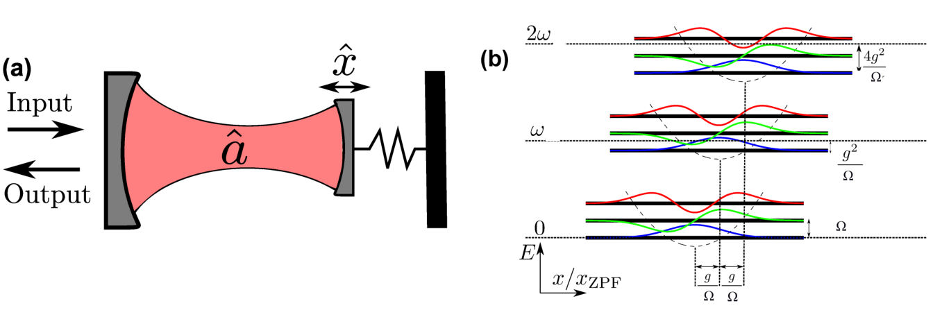
In 2011, Rabl reported on the occurrence of photon blockade (see sec. 2.3.3 for a discussion in terms of the JC dynamics), ascertained from photon antibunching in coincidence measurements on the output of a weakly-driven optomechanical system Rabl 2011. Concurrently, Nunenkamp and coworkers focused on the consequences of the single-photon strong-coupling regime , allowing radiation pressure of a single photon to displace the mechanical oscillator by more than its zero-point uncertainty. They showed that in this regime the power spectrum has multiple sidebands and that the cavity response has several resonances in the resolved-sideband limit Nunnenkamp et al. 2011a. The nonlinear quantum Langevin equations are solved in the weak-drive limit after diagonalizing the optomechanical Hamiltonian (805) via the polaron transformation with [see also eq. (223)]. The mean intracavity photon number in the steady state evinces a series of resonance peaks spaced apart by the mechanical frequency :
| (817) |
where is the thermal occupation of the mechanical bath, are the dissipation rates for the optical mode and the mechanical system, respectively, and is the mean photon number on resonance in the cavity (with the coherent amplitude of the input light). For only terms with contribute, and we find that the resonance peaks are weighted by a Poisson distribution of variance and have widths . The resonances occur if the laser frequency matches the frequency difference between the vacuum state and the manifold of the one-photon eigenstates , satisfying , while the Poisson weights originate from the Franck-Condon factors [see also the Hamiltonian spectrum depicted in fig. 77(b)]
| (818) |
Moreover, for , multiphoton transitions occur between the vacuum state and the lowest-energy -photon state (since ) and the system is in the Franck-Condon blockade regime with all intermediate transitions being off-resonant. In 2015, a design of cavity optomechanics in the microwave frequency regime was proposed, involving a Josephson junction qubit; the radiation-pressure interaction was enhanced by six orders of magnitude, accessing the strong-coupling regime Pirkkalainen et al. 2015.
Elste et al. Elste et al. 2009 proposed a novel kind of optomechanics, where the mechanical motion modulates the linewidth of the cavity. In this case, the radiation pressure force spectrum features a Fano resonance, substantially modifying the interaction between light and mechanical degrees of freedom. The potential of dissipative optomechanics as a source for producing squeezed light and correlated photons was explored in Kilda and Nunnenkamp 2015.
We should also add here a short comment on dispersive optomechanics, focusing on a so-called ‘membrane in the middle’ of a cavity configuration Jayich et al. 2008. Such an optomechanical device can be operated in a regime where the cavity frequency depends directly on –the position squared of the macroscopic mechanical oscillator. As a consequence, the experimenter can perform a direct measurement to determine the energy of the oscillator, , where is the number of phonons in the state of the membrane Thompson et al. 2008a. If the cavity is driven on resonance, the phase of the transmitted beam is proportional to the energy . Such a measurement allows the detection of energy quantization, something which is not possible with a cavity whose frequency directly depends on . Such a linear-position detection, like the ones we have discussed above in this section, is limited by quantum backaction Braginsky and Khalili 1996.
Controlling the external degree of freedom of trapped molecular ions to eliminate systematic effects such as Doppler shifts is paramount for their applications to spectroscopy, precision measurements of fundamental constants, and quantum information technology. The experiment conducted by Qi and collaborators Qi et al. 2023 has recently attained near ground-state cooling of the axial motional modes of a calcium mono-oxide ion via sympathetic sideband cooling with a co-trapped calcium ion Kielpinski et al. 2000 [see also the ion-cooling experiments discussed in sec. 5.4]. Remarkably, the phonon state of the axial out-of-phase mode of the ion chain has been preserved as the mode frequency is adiabatically varied. In the sub-field of active optomechanics, where the energy source is the intracavity active medium, the motion of a mechanical oscillator may be also detected by measuring the laser intensity, spectral broadening, and laser frequency stability Yu and Vollmer 2022.
The ability to achieve coherent quantum control over the center of mass motion of massive mechanical objects provides a powerful scheme to conduct experiments to assess the foundations of quantum theory Kippenberg and Vahala 2008; Aspelmeyer et al. 2014a. Optomechanical systems are also very good candidates for detecting quantum signatures of gravity. The models of Karolyhazy 1966; Diósi 1984; Penrose 1996 identify gravity as the dominant agent of the state-vector collapse. A notable example in a different direction is provided in Pikovski et al. 2012, where a protocol is proposed using quantum optical control and readout of a mechanical system to probe possible deviations from the quantum commutation relation even at the Planck scale.
7.6.2 Cavity optomechanics II: Photon-phonon interaction formulated as a scattering problem
Quantum optics experiments are scattering experiments, where the experimenter controls the applied inputs and measures the generated outputs. We will now formalize further the photon-phonon interaction as a scattering problem, following closely the analysis of Maurer et al. 2023a where the motional quantum dynamics of a levitated dielectric sphere interacting with the quantum electromagnetic field are discussed beyond the point-dipole approximation. The Hamiltonian is formulated under the assumption that the dielectric sphere of mass primarily interacts only with electromagnetic field modes in a sufficiently narrow frequency window, so that its electromagnetic response can be described by a single scalar and real relative permittivity . For sufficiently small center-of-mass displacements, meaning that the standard deviation is smaller than any relevant length scale associated with the variation of the electromagnetic field, the total Hamiltonian describing the interaction between the center-of-mass motion and the electromagnetic field – whose deterministic part generates the conservative confining potential – reads
| (819) |
where is the radiation-pressure force operator, which does not commute with the Hamiltonian describing the free evolution of the electromagnetic field. From the Hamiltonian (819), the Heisenberg equation of motion for the -component of the center-of-mass position vector is
| (820) |
where is the corresponding frequency of the (anisotropic) harmonic trap. The right-hand side of eq. (820) is the radiation pressure exerted by self-consistent electromagnetic fields, expressed as a surface integral of the Maxwell stress tensor in the far field of the dielectric sphere and defined as
| (821) |
The electric and magnetic field operators can be expanded in terms of the normalized eigenmodes for a scattering problem where the sphere is motionless and placed at the origin of coordinates,
| (822a) | ||||
| (822b) | ||||
where the normalized scattering eigenmodes are labeled by the multi-index , with the polarization index and the wavevector. They comprise a plane-wave contribution alongside an elastically-scattered field off the dielectric sphere. All the elastic scattering processes arise as solutions of the Lorenz-Mie problem Mie 1908; Maurer et al. 2023b. Now, expressing the Hamiltonian (819) in terms of photons interacting with center-of-mass phonons, we may write
| (823) |
The third term accounts for the two fundamental processes that make the optomechanical light-matter interaction: (i) Stokes processes where a photon in mode is inelastically scattered into a lower-frequency photon in mode by generating a phonon in mode , and (ii) anti-Stokes processes where a photon in mode is inelastically scattered into a higher-frequency photon in mode by absorbing a phonon in mode . The photon-phonon interaction is captured by the coupling rates , which can be written as a surface integral of a far-field quantity depending on the normalized scattering eigenmodes:
| (824) |
containing products of vector spherical harmonics Neves and Cesar 2019 and expressed as a sum of discrete angular momentum states with and polarization indicating TE or TM modes.
We will now specialize to the case where some of the electromagnetic field modes are in a coherent state, given by
| (825) |
with an associated electric field
| (826) |
Assuming that all modes found in the coherent state generated by a monochromatic laser have the same frequency , the linearized Hamiltonian accounting for the fluctuations of the electromagnetic field about in a frame rotating with is given by
| (827) |
where and . For example, in the case of a single Gaussian beam propagating along the positive -axis with a focus at the origin of co-ordinates, the corresponding coherent amplitudes for each polarization are
| (828) |
where is the optical power of the focused field, is the numerical aperture of the lens, and is the filling factor over the lens, guaranteeing maximum focusing of the beam Novotny and Hecht 2012.
![[Uncaptioned image]](2202.00330v4/OptSc1.png)
![[Uncaptioned image]](2202.00330v4/OptSc2.png)
![[Uncaptioned image]](2202.00330v4/OptSc3.png)
The linearized Hamiltonian of eq. (827), modeling both Stokes and anti-Stokes processes as depicted in fig. 78(a), describes two important phenomena: (a) the laser-light recoil heating (dissipation of the center-of-mass motion) and (b) the scattering of light from the dielectric sphere, yielding information on the position fluctuation of the center of mass. The angular distribution of the scattered light is termed information radiation pattern (IRP), which will be determined below through the scattering amplitudes.
The transition amplitudes associated with these processes are evaluated with respect to the input and output states as
| (829) |
The input is formed by the product state (the first component refers to the center-of-mass degrees of freedom with ), while the output state is and for the Stokes and anti-Stokes transitions, respectively. The time-evolution operator is given as , where is the Hamiltonian (819). For to be nonzero, the incoming photon must belong to a mode excited by the classical electromagnetic field, whereas the photon scattered into the mode may belong to any of the available electromagnetic field modes.
Using Fermi’s golden rule, one may calculate the transition probability rates for the two processes under consideration in the asymptotic limit as
| (830a) | |||
| (830b) | |||
where
| (831) |
Since the linearized couplings extend over a broad frequency range set by , we may consider
| (832) |
The above equality does not hold in environments that modify the mode structure of the electromagnetic field.
The optical configuration is displayed in fig. 78(b). Photon scattering via Stokes () or anti-Stokes () processes yields information about the center-of-mass motion about a particular axis via the information radiation pattern (IRP)
| (833) |
a normalized quantity providing the solid-angle probability distribution of a photon scattered either through a Stokes or an anti-Stokes process. In the broadband coupling regime, the IRP is the same for both Stokes and anti-Stokes processes, which means that these can be distinguished by means of the frequency of a scattered photon but not its angular distribution.
The determination of the laser recoil heating rate and the IRP – both of which can be derived from the coupling rates and the coherent-state amplitudes associated with a classical electromagnetic field in a linearized treatment – is indispensable for the implementation of active feedback cooling through optical detection Magrini et al. 2021; Tebbenjohanns et al. 2021; Kamba et al. 2022. In the experiment of Tebbenjohanns et al. 2021, in particular, a silica nanoparticle is optically levitated in a cryogenic environment. The light scattered off the particle in the backwards direction is split between heterodyne and homodyne receivers. A linear filter then processes the homodyne signal and feeds it back to the trap in the form of a Coulomb force exerted to the charged particle in order to cool its centre-of-mass motion along the optical axis. The minimum attainable phonon-occupation number is given by the formula
| (834) |
where denotes the total efficiency of the cooling. It is formed by the product of three individual efficiencies: the detection efficiency
| (835) |
evaluated over the solid angle subtended by the collection lens [see figs. 78(c, d)], the efficiency associated with information loss to the environment,
| (836) |
where is the heating rate due to the presence of the environmental gas at pressure and temperature . The last term in the product making the total efficiency is an efficiency coefficient amassing the contribution from all other information channels in the active feedback scheme. Scattering of a two-photon state off a dielectric sphere leads to a vanishing simultaneous joint detection probability of the two scattered photons along diagonal stripes in the second-order correlation function due to the Hong-Ou-Mandel interference Maurer et al. 2023b. Tuneable interactions between different mechanical modes mediated by photons scattered by spatially separated particles have been recently demonstrated in the experiment of Vijayan et al. 2024, where measured spectrograms reveal the normal mode splittings arising from cavity mediated particle-particle interactions for different values of the cavity detuning.
7.6.3 Coherent interaction of a magnon and a qubit
The collective bosonic spin excitations of magnets are called magnons. An anisotropic ferromagnet can host magnons with a controllable degree of intrinsic squeezing in equilibrium, while exchange-coupling a single qubit with this ferromagnet can realize the quantum Rabi model. In the limit of zero anisotropy, the mapping reduces to the JC Hamiltonian.
Ferromagnetic films often exhibit strong shape anisotropy on top of magnetocrystalline anisotropies Kamra and Belzig 2016a. These effects are modeled by including a single-ion anisotropy contribution to the isotropic terms. We consider a spin model (where the spin operator at lattice site is denoted by ) with nearest-neighbor interactions (the sum over which is indicated by ). The total spin Hamiltonian in a ferromagnet of lattice sites includes the Zeeman energy induced by an external magnetic field (taken along the direction of the -axis), the exchange interaction between nearest neighbors and a possible (generalized) anisotropy term:
| (837) |
where is the gyromagnetic ratio, is the applied external field in the direction of the -axis and is the exchange coupling strength . The coefficients , and characterize the magnetic anisotropy Skogvoll et al. 2021; Kamra and Belzig 2016b; Römling et al. 2023. Assuming only small deviations from the ground state, where the spins point in the direction owing to a dominant Zeeman-energy contribution, we can operate under the spin wave approximation Auerbach 1994b using the Holstein-Primakoff transformations Holstein and Primakoff 1940
| (838) |
where and stands for the magnitude of the spin (see also the application of these transformations to derived the ’bosonised Dicke Hamiltonian’ (324) in sec. 2.5.5). The bosonic magnon operator – defined in the context of the above transformation – creates a “spin flip” at lattice site . Taking the corresponding Fourier transform we write
| (839) |
Using the Holstein-Primakoff relations (838) and the Fourier decomposition, and retaining only the magnon mode with by focusing on coherent resonant interactions, it can be shown Skogvoll et al. 2021 that the ferromagnetic Hamiltonian (837) is recast into the form
| (840) |
where . The constant reflects the impact of the external magnetic field, while the constant directly reflects the transverse anisotropy as . The Hamiltonian (840) can be diagonalized via a Bogoliubov transformation, defining a so-called bare squeezed magnon:
| (841) |
and the single-mode squeeze operator , defined in eq. (238), employed in the transformation
| (842) |
The diagonalized Hamiltonian then reads
| (843) |
which sets and as requirements for stability. A uniformly ordered ground state can be maintained for a sufficiently large applied magnetic field . In typical experiments, it is shown that Kamra and Belzig 2016a; Kamra and Belzig 2016b.
Having noted the link between anisotropy and squeezing, let us now see how the dipolar interaction of a single qubit with the ferromagnet can lead to coherent dynamics described by a Jaynes-Cummings Hamiltonian Skogvoll et al. 2021; Trifunovic et al. 2013. The interfacial exchange interaction is parametrized via the operator
| (844) |
where labels the interfacial site. The ferromagnetic spin represented by the operator is coupled to the electronic states comprising the qubit of spin , with the interfacial coupling strength . The qubit spin can be expressed in terms of the Pauli matrices as , where is the spatial wavefunction amplitude of the qubit orbital at position , and . Writing the interfacial interaction in the form of a central spin model (see sec. 2.5.7)
| (845) |
using the Fourier decomposition and the Holstein-Primakoff relations, and retaining only the uniform magnon mode (), we find that the term in parentheses describes a coherent interaction between the magnon and the qubit, which can be expressed as
| (846) |
In the above formula, is the wavefunction averaged over the interfacial sites. Breaking the symmetry in the plane transverse to the equilibrium spin order generates squeezing, while a uniaxial anisotropy does not. For this configuration one obtains Skogvoll et al. 2021
| (847) |
showing that the squeeze parameter controls the relative importance of the rotating and counter-rotating terms. The coupling strengths can also reach the deep-strong regime. The composite nature of the squeezed magnon enables a simultaneous excitation of three spin qubits coupled to the same ferromagnet. This allows for the robust generation of three-qubit Greenberger-Horne-Zeilinger (GHZ) and related states Skogvoll et al. 2021 needed for implementing Shor’s quantum error-correction code Shor 1995; Neeley et al. 2010; DiCarlo et al. 2010; Reed et al. 2012.
Finally, summing over non-uniform modes, the first term in eq. (845) can be recast in the form
| (848) |
The first term amounts to a mere renormalization of the qubit frequency, and assuming to be spatially independent we may sum over the interfacial sites to obtain
| (849) |
Limiting once again our attention to the uniform magnon mode, we end up in an effective dispersive interaction of the form Römling et al. 2023, which we have already met in sec. 4.2.
Following up our discussion in secs. 2.4 and 2.5, we note that a hybrid quantum system, consisting of a single-mode cavity simultaneously coupled to both a two-level system and an yttrium-iron-garnet (YIG) sphere supporting magnons with Kerr nonlinearity has recently been proposed to restore the supperradiant phase transition against the term Liu et al. 2023b. It is found that the Kerr-magnon-induced phase transition can occur in both cases of ignoring and including the intrinsic diamagnetic term. Regarding now extended systems, a central element in an array of YIG spheres coupled to identical lossy cavity modes is driven by an external quantum squeezed drive in a magnon-magnon entanglement generation scheme proposed to generate bipartite and tripartite entanglement between distant magnon modes across the entire array Ullah et al. 2023.
7.6.4 Further hybrid setups
According to the proposal of Pályi et al. 2012, a quantum dot with an odd number of electrons can be modelled by the Jaynes-Cummings Hamiltonian in the strong-coupling regime. A quantized flexural mode of the suspended tube plays the role of the optical mode while two distinct two-level subspaces – for small and large magnetic fields – can be modelled by two-state atoms in this nanomechanical setup. The authors start from the Hamiltonian
| (850) |
where and are the spin-orbit and intervalley couplings, and () are the Pauli matrices for the valley and spin degrees of freedom, is the tangent vector along the carbon nanotube (CNT) axis, and denotes the applied magnetic field.
A generic deformation of the CNT with deflection makes the tangent vector coordinate-dependent. Expanding for small deflections, we rewrite the coupling terms in Hamiltonian (850)) as and . The deflection is then expressed in terms of the creation and annihilation operators and for a quantized flexural phonon mode, , where and are the waveform and zero-point amplitude of the phonon mode. Then, each of the three qubit types (spin, spin-valley qubits) acquires a coupling to the oscillator mode which can be modeled as
| (851) |
In the above Hamiltonian, a term describing external driving of the oscillator with frequency and coupling strength has been included, which can be achieved by coupling to the ac electric field of a nearby antenna. The coupling strength is directly proportional to as well as to the derivative of the waveform corresponding to the phonon mode averaged against the electron density profile in the quantum dot. Upon effecting the RWA, the authors employ the standard master equation in Lindblad form to study strong-coupling conditions at finite temperatures.
An optomechanical setup consisting of a laser-pumped cavity partitioned by a flexible membrane which is partially transmissive to light, and thereby subject to radiation pressure, has been proposed as a comparison to the critical behaviour encountered in the Dicke model Mumford et al. 2015. This proposal follows the consideration of a Fabry-Pérot cavity with a moveable mirror to realize the Dicke–Hepp–Lieb phase transition in Bhattacherjee 2013. The authors report on a new type of superradiance effect in this system for a very low value of the coupling between the optical and mechanical mode.
The simplest many-body description for bosons in a double-well potential is the single-band two-site Bose-Hubbard model. For a small overlap between the two condensates the ground state is a macroscopic Schrödinger cat state Cirac et al. 1998. The “size of the cat” is inversely proportional to the overlap. With the addition of an atomic impurity, the Hamiltonian of the system reads
| (852) |
Here, is the number difference operator between the two wells confining the bosons, and is the boson hopping operator responsible for the coherence between the two wells. Likewise, and are the equivalent operators for the impurity. We assume that both the boson and impurity creation/annihilation operators obey the standard bosonic commutation relations, i.e., with and all the remaining commutators are identically zero. parametrizes the boson-impurity interaction, while and are the hopping amplitudes for the bosons and the impurity, respectively. Using similar notation, and are the respective differences between the zero-point energies of the two wells, i.e., the tilt for the bosons and the impurity.
The Hamiltonian of eq. (852) can be recast in a simpler form via a spin notation which makes use of the symmetric/antisymmetric (S/AS) modes instead of the left/right (L/R) modes as a basis. The S/AS modes are the eigenmodes of the single-particle problem, i.e., in the absence of interactions. Therefore, in the limit , the ground state corresponds to all the particles belonging to the S mode, since it has a lower energy. Using a simple Hadamard rotation of the L/R creation (annihilation) operators we have,
| (853) | |||||
| (854) |
and similar expressions hold for the impurity operators. In the new basis, and for vanishing tilts , eq. (852) takes the form
| (855) |
where we have used the Schwinger spin representation Sakurai 1994, i.e., and . Apart from the trivial symmetry related to particle conservation, we note that the Hamiltonian supports a parity symmetry under the transformation , , , and likewise for the impurity spin operators. This spin rotation preserves the angular momentum commutation relations. Note that in the original L/R-basis this symmetry is nothing but a reflection of the double-well about the origin. It follows that a non-zero tilt or breaks this symmetry.
The model Hamiltonian written in the form of eq. (855) shows some resemblance to the Dicke Hamiltonian
| (856) |
Here, are photon, i.e., bosonic creation (annihilation) operators and and are spin operators. eq. (856) describes a spin- system coupled to the position coordinate of a harmonic oscillator. The frequencies and are the spin precession and harmonic oscillator frequencies, respectively, and is the coupling strength. As we have seen many times so far, this system experiences a QPT at a certain critical value Mumford et al. 2014. Meanwhile, the semiclassical dynamical behaviour of a fermionic condensate interacting with a single bosonic mode is studied via a generalization of the Tavis-Cummings model in Yuzbashyan et al. 2005.
Collapses and revivals typical of the JC dynamics can be observed in the regime of perfect Rydberg blockade where the mesoscopic atomic ensemble is effectively a two-level system with two levels represented by collective Dicke states, say and . The ‘atom’ is initially prepared in the state , and the field is in state , where the probability to find photons in the field mode is . The number of photons in a coherent state of the electromagnetic field (with average photon number ) follows the Poissonian distribution Loudon 1983,
| (857) |
Following up our discussion from sec. 2.2.2, we note that the solution of Schrödinger’s equation yields the probability to find the atom in the excited state Gea-Banacloche 1990b,
| (858) |
The familiar dependence in eq. (858) arises from matrix elements of creation and annihilation operators. Similarly, due to the dependence of the Rabi frequency of single-atom excitation in Rydberg-blockaded ensembles on the number of atoms, the probability of single-atom excitation in an ensemble with a random number of atoms is given by
| (859) |
where is the probability to have atoms in the ensemble. Given the similarity between eqs. (858) and (859), one can introduce a new quantum number for the mesoscospic ensemble of atoms which is equivalent to the number of photons and is described by similar annihilation and creation operators Beterov et al. 2014. Moving on to a hybrid system of ultracold atoms in interaction with the field of waveguide resonators, coherent coupling of a Rydberg transition of atoms trapped inside an integrated superconducting chip to the microwave field of an on-chip coplanar waveguide resonator has been very recently reported in Kaiser et al. 2022. The setup supports cavity-driven Rabi oscillations between a pair of Rydberg states of atoms in an inhomogeneous electric field near the atom chip surface.
The photonic realization of the quantum Rabi model in a Hilbert space, based on a semi-infinite curved binary waveguide array, was analyzed in Crespi et al. 2012. The experiment and the accompanying simulations were performed in the deep strong-coupling regime (). In the limit where the qubit frequency tends to zero, strictly periodic temporal dynamics of photon number distribution were observed, with the periodicity dictated by the frequency of the quantized field. Alternatively, for a cloud of ultracold atoms subjected to two laser-induced potentials, a periodic lattice and a harmonic trap, when the system state which is fully contained in the first Brillouin zone the system Hamiltonian can be mapped to the quantum Rabi model in terms of the momentum operator and in a rotated spin basis Felicetti et al. 2017. Similarly, the anisotropic 1D spin-orbit coupling realized in a trapped cold atomic gas has been mapped to the quantum Rabi model with spin-momentum coupling in Hu and Chen 2013. The energy spectrum is extracted from the zeros of a transcendental equation in the spirit of Braak 2011.
Reporting from the experimental front once again, a hybrid quantum system that combines two heterogeneous collective-excitation modes -- a narrow-linewidth magnetostatic mode and a superconducting qubit – was modeled by a JC-type Hamiltonian to interpret the normal-mode splitting arising due to strong coupling between the qubit and the magnon Tabuchi et al. 2015. A couple of years later, magnon number states were resolved by employing a qubit dispersively coupled to a harmonic oscillator for the experiment reported in Lachance-Quirion et al. 2017. At the same time, two-level hybrid-spin qubits can be defined using magnetic dipole coupling of an ensemble of spins to microstrip cavities with an embedded nonlinear subsystem such as a transmon qubit Imamoğlu 2009.
We conclude this section with a brief reference to solid-state devices and models that have been of paramount importance throughout the last two decades up to our days. The cyclotron motion in graphene monolayers positioned perpendicular to a magnetic field is described by a Hamiltonian which is formally equivalent to the JC model Schliemann 2008. Within that correspondence, the solution for the time-dependent position operators in the Heisenberg picture is considerably simplified if one assumes that the electron energy is larger than the characteristic energy scale of the Hamiltonian, set by the magnetic length and the Fermi velocity in graphene. In connection to graphene and its relativistic Landau levels, and anti-JC term arises when modelling the quantum Hall effect in square lattice subjected to a non-Abelian gauge potential Goldman et al. 2009. Fermionic degrees of freedom are also involved in the edge dynamics of a spin-Hall insulator interacting with circularly polarized quantized electromagnetic field through a Zeeman term were considered in Gulácsi and Dóra 2015. The pertinent Hamiltonian reads
| (860) |
Here, is the Fermi velocity of the edge state, and denote the resonance frequency and annihilation operator of the cavity mode, while annihilates an electron with momentum and spin . The last term describes the Zeeman interaction with the spin operators expressed as and . The Zeeman coupling depends on the photon frequency as . Considering a single momentum , the Hamiltonian reduces to the Jaynes-Cummings model. Hence, the spectrum consists of the energy doublet
| (861) |
with being a positive integer, plus a single mode . The Purcell enhancement factor and the excited-state population dynamics for a quantum emitter in the vicinity of a graphene nanodisk were calculated in Thanopulos et al. 2022, and distinct signatures of non-Markovianity were identified.
A very recent notable proposal in solid-state quantum technology concerns the use of nuclear spin states of magnetic ions. The hyperfine interaction with an electronic spin mediates the coupling of nuclear spins to to electromagnetic radiation, enhancing the nuclear Rabi frequencies with respect to those of isolated nuclei Hussain et al. 2018. This enhancement can be of use when exploring the coupling of on-chip superconducting resonators to the nuclear spins of magnetic molecules Gaita-Ariño et al. 2019. Avoided crossings have been experimentally observed when the level splittings of 171Yb and 173Yb are brought into resonance with the cavity photons Rollano et al. 2022.
Furthermore, we mention that Sommerfeld’s theory Sommerfeld 1928 of the free electron gas has been revisited in the framework of cavity quantum electrodynamics. Rokaj and coworkers find that the electron-photon ground state is a Fermi liquid containing virtual photons. In contrast to models of finite systems, no ground state exists if the diamagentic term is omitted. Furthermore, linear response theory shows that the cavity field induces plasmon-polariton excitations, and alters the optical and the DC conductivity of the electron gas Rokaj et al. 2022. Furthermore, The Tavis-Cummings Hamiltonian has been used in Lei et al. 2023 to model an inhomogeneously broadened ensemble of solid-state emitters coupled with high cooperativity to a nanophotonic resonator under strong excitation. A collectively induced transparency in the cavity reflection spectrum results from quantum interference as a collective effect, while the coherent excitation of the system produces a nonlinear response spanning a broad range from subradiance to superradiance.
Opening a new path, Karnieli and coworkers have developed a unified theory to account for the quantum three-particle interaction of a free electron, a bound electron, and a photon in a single-mode resonator Karnieli et al. 2023. Modeling the bound-electron system by a two-state atom, they are able to reduce the problem to the JC interaction and the free-electron bound-electron resonant interaction models for the coupling to the cavity field and the free electron, respectively. The coupling between the free electron and the cavity field is generally captured by the quantum photon–induced near-field electron microscopy model . This simplified formulation can be extended to include a wide range of models for the emitter-cavity system, including the quantum Rabi model for ultrastrong light-matter coupling, the Dicke model for an ensemble of emitters, or the Hopfield model for collective matter excitations. The latter may replace the JC model, e.g, in dielectric micro- and nanocavities, accounting for a larger Rabi splitting.
8 Extensions to many-body configurations and additional degrees of freedom
Some years after the millennium, we saw the first realization of the Mott-insulator phase transition in an ultracold atomic system Greiner et al. 2002. This was a breakthrough demonstrating how truly strongly interacting many-body quantum systems could be studied in a quantum optical setting. These systems had a clear advantage over many other systems in the condensed matter community due to their flexibility and controllability. This spurred the quest for realizing quantum simulators, i.e., controllable quantum systems mimicking other quantum systems which are not subject to the same control and are too complicated to be simulated on a classical computer. Apart from being capable of realizing known many-body systems from (mainly) the condensed-matter physics community, these atomic setups also enable the study of novel systems lacking counterparts in other communities. An avalanche of experimental and theoretical activities set off, and it did not take long before new proposals of different systems implementing quantum simulators popped up Carusotto and Ciuti 2013; Georgescu et al. 2014. In 2006, two notable works suggested how one may simulate interacting many-body systems with photons Hartmann et al. 2006a; Greentree et al. 2006a. Following in particular the footsteps of the development of circuit QED (see section 4), it was explained how to couple Jaynes-Cummings (JC) sub-systems into a lattice—the Jaynes-Cummings-Hubbard model: each JC sub-system, comprising a qubit and a photon mode, becomes connected by allowing for photons to tunnel between neighboring JC systems. The JC nonlinearity induces the effective interaction, and it was argued how the strongly-correlated regime could be reached making truly ‘many-body’ systems beyond the perturbative regime. Another feature of interest, not as important for ultracold atoms in optical lattices, is the nonequilibrium character of the system; typically one has in mind driven-dissipative resonators. These types of systems will be discussed in sec. 8.1 below. Roughly at the same time, people started to think what new physics will emerge by coupling condensed atoms to a single mode of an optical resonator Brennecke et al. 2007; Colombe et al. 2007. We have already seen two phenomena where the atom number plays an important role; in sec. 3.1.1 we discussed optical bistability and how the coupling of thermal atomic gases to the cavity field may cause a bistable behaviour, and in sec 2.5.5 the superradiance was considered. By lowering the temperature of the atomic gas such that the atoms condense, a new regime is reached where the typical atomic kinetic energy, set by the recoil energy , becomes comparable to other energy scales, see sec. 2.5.4. In a condensate, contrary to a thermal gas, we expect long-range order meaning that the atomic gas shows quantum coherence over large spatial distances, and it makes sense to talk about collective excitation modes of the condensate rather than individual atomic excitations. An important ingredient in these systems, which are discussed in sec. 8.2, that makes them different from other ultracold atomic setups, is the infinite-range interaction between the atoms stemming from the common coupling to the quantized light field in the cavity. This leads to, as we will show, a set of novel phenomena. Finally, in this section we also discuss a relatively young field where one lets a gas of molecules, rather than atoms, be coherently coupled to optical resonators. While not condensed, the molecular cavity QED setting still adds a complexity in terms of the internal molecular structures. In a Born-Oppenheimer picture, the electronic transition frequencies are set by the internuclear distances, which of course are dynamical degrees of freedom. Thus, apart from the energy exchange between electronic transitions and photons, we also derive results concerning transitions in the molecular vibrations. One idea is that ‘dressing the molecules’ with the cavity photons can alter chemical reactions, and thereby control them to some extent.
8.1 Jaynes-Cummings-Hubbard models
The Jaynes-Cummings Hubbard (JCH) Hamiltonian was formulated to describe an optical system displaying strong correlations on a mesoscopic scale; in other words, we are dealing with a model imitating equilibrium predictions in situations where the photon number is not conserved. The original setup, proposed in 2006 Greentree et al. 2006b, comprised a two-dimensional array of connected cavities coupled to two-level atoms such that photon blockade occurs, which means that absorption of one photon and the formation of a vacuum Rabi resonance ‘‘blocks’’ the absorption of a second. This behavior is generalized to multiphoton resonances which, however, do not present an absolute barrier to the absorption of additional photons since, in a nonequilibrium configuration, the coherent drive strength broadens the energy levels Carmichael 2015. Onsite JC interactions with photon hopping between cavities and an appropriate chemical-potential term comprise the JCH Hamiltonian,
| (862) |
where are the hopping coefficients, is the total (photonic and atomic) excitation number operator at site (where commutes with ), associated with the chemical potential . Assuming zero disorder, introducing a superfluid order parameter , and applying the decoupling transformation , results in the mean-field single-site Hamiltonian
| (863) |
where is the number of nearest neighbors, between which inter-cavity hopping occurs with frequency . When the order parameter is zero (), one encounters a Mott phase with a fixed number of excitations per site in the absence of fluctuations; the presence of a finite order parameter, , on the other hand, indicates a superfluid phase.
The extent of the characteristic Mott-insulator lobes is determined by an appropriate boundary set by the critical chemical potential; such a potential corresponds to the increment of the excitation per site by one, yielding
| (864) |
where now we have taken into account a detuning between the onsite coupled cavity mode and two-level atom , featuring in the familiar Rabi frequencies . The phase diagram is depicted in fig. 79 (a).


The number of excitations per site, , in each lobe of the Mott-insulator phase has been computed post-minimization for the ground state, following the expression as a function of and in a grand-canonical ensemble formulation. The produced plateaus point to regimes of constant density and incompressibility, attributed to the gapped Mott-insulator phase. In Greentree et al. 2006b, negatively-charged NV centers, placed inside each cavity of the ensemble, have been proposed as a promising candidate for realizing this equilibrium quantum phase transition of light.
The Bose-Hubbard Hamiltonian and the corresponding two phases of matter has been associated with hopping of cavity polaritons due to the mode-profile overlap of adjacent resonators. Atoms coupled to the intracavity modes are driven by external detuned coherent fields Hartmann et al. 2006b. To generate repulsion between polaritons, four-level atoms are driven in such a fashion to emulate Electromagnetically Induced Transparency Werner and Imamoḡlu 1999. With reference to the level-structure of fig. 79, in a frame rotating with the Hamiltonian
the interaction Hamiltonian of the atoms coupled to the cavity mode reads
| (865) |
where the operator projects the level to the level of the atom, is the cavity resonance frequency, is the Rabi frequency determined by the laser driving, and are the dipole coupling strengths of the cavity mode to the respective atomic transitions.
We are interested in the situations where there is on average one excitation per cavity; hence, we consider states with at most two excitations per cavity, suppressed by a Kerr nonlinearity. Neglecting two-photon detuned transitions and the coupling to the atomic level 4 Rebić et al. 2002, as illustrated in fig. 79 (b), the Hamiltonian of eq. (865) can be reduced to include interactions between three species of polaritons when the number of atoms is large (). These polaritons, i.e., quasi particles formed by an atomic and a photonic contribution, are created by three operators, denoted by , in the subspace of at most two excitations. After defining collective spin operators and alongside the renormalized coupling rates , and , the aforementioned creation operators assume the form
| (866) |
These operators satisfy the familiar bosonic commutation relations , , with . For and , the Hamiltonian of eq. (865) is then reduced to
| (867) |
with new frequencies , . We now need to write the full interaction Hamiltonian in the polariton basis, expressing the operators and in terms of , and decoupling the fourth level from the dynamics. In the two-excitation manifold and the rotating-wave approximation, we express the coupling of the polaritons to the level in question as
where . In a frame rotating with respect to the Hamiltonian of eq. (867), the operator rotates at the frequency . In the hierarchy of timescales set by
| (868) |
we neglect all terms rotating with the frequencies , , which amounts to eliminating the interactions coupling and to the remaining polaritons. If we further assume that , the presence of the fourth level results only in an energy shift of , where (see eq. 5 of Werner and Imamoḡlu 1999)
| (869) |
A state containing one excitation of the operator comes with a probability , which determines an effective decay rate for the polariton species via the route of spontaneous emission from the fourth level. Similarly, the two-photon detuning is responsible for an energy shift , playing the role of a chemical potential in the resulting effective Hamiltonian in the perturbative regime,
| (870) |
which is the normally-ordered Hamiltonian of the nonlinear polarizability model Drummond and Walls 1980b —the second term accounting for the Kerr nonlinearity and the associated repulsion. Photon loss at a rate and spontaneous emission from the fourth atomic level at a rate lead to the following decoherence rate
| (871) |
To close this subsection out, we mention that a trapped-ion quantum simulator with up to 32 ions has been used to study the transition from Markovian to non-Markovian spin dynamics in different regimes of the JCH model, tuning the spin frequencies to different locations of the phonon band. In addition, collapse and revival signals provide evidence for the occurrence of localization Li et al. 2022f. The ground state quantum phase transition in the Rabi-Hubbard model has been experimentally observed via a slow quench of the coupling strength once again in a system of trapped ions, while the dynamical evolution for average spin inversion, phonon number and entanglement entropy is displayed for a set of parameter regimes in Mei et al. 2022.
An array of coupled cavities in the photon blockade regime can be mapped to the transverse-field anisotropic model Bardyn and İmamoǧlu 2012 (see also subsec. 5.4). Two-time correlations leading to the absorption and fluorescence spectra for such an array were calculated in Kilda and Keeling 2019; Kilda 2020. The structure of the distribution function, calculated by the applying the fluctuation dissipation theorem Breuer and Petruccione 2002; Sieberer et al. 2016a, and the associated thermalization can be understood by using a spin-wave theory, while the Fourier-transform of fluorescence in momentum space reveals the nature of quasiparticle excitations in the quasithermal state.
8.2 Many-body cavity QED
In sec. 2.5.4, we saw that as the atomic kinetic energy is lowered, the motional states of the atoms couple to the other degrees of freedom via absorption/emission of cavity photons. This implies the alteration of their kinetic energy by one recoil-energy unit, , introduced in that subsection (here we also define the recoil frequency ). By ‘‘many-body cavity QED’’ we envisage a large number of ultracold atoms coherently coupled to the cavity mode Ritsch et al. 2013; Mivehvar et al. 2021. Thus, in this section the motional degrees of freedom are considered, while they were not taken into account when discussing the TC and Dicke models in sec. 2.5.5. Instead of coupling the individual atomic kinetic energies to the light field, it is often more convenient to think in terms of collective effects where low-energy phonon modes of the atomic cloud interact with the photons Ritsch et al. 2013; Mivehvar et al. 2021. These collective modes become relevant once the atoms are condensed and coherences extend over the full atomic cloud Pethick and Smith 2008. At these low temperatures an additional effect that may arise is that of atom-atom interaction, which may indeed qualitatively modify the picture Lewenstein et al. 2007a; Bloch et al. 2008a.
With the development of experimental techniques in laser cooling and trapping of neutral atoms it became feasible to also couple a gas of ultracold, or even condensed, atoms to the cavity field. In these first pioneering experiments, the collective ultrastrong coupling regime of a large number of two-level atoms was demonstrated in two back-to-back papers by the ETH group of T. Esslinger Brennecke et al. 2007 and the ENS group of J. Reichel Colombe et al. 2007. The square-root dependence of the collective coupling on the number of atoms, , was verified in both experiments. The reason why the coupling scales as and not simply as can be found in the construction of the Dicke states (61). This is similar to the enhancement of collective spontaneous emission – the superradiance we discussed in sec. 2.5.5. In a strict sense, for the results of these works it was not crucial that the atoms were condensed. Nevertheless, at least in the ETH experiment, condensation was confirmed. After these experiments, a couple of independent experimental works on optical bistability followed, in Fabry-Pérot cavities Gupta et al. 2007; Brennecke et al. 2008 and in a ring cavity Schmidt et al. 2014. It turned out that these systems were excellent candidates for studying optomechanics Brooks et al. 2012, i.e. the coupling between light and mechanical modes we discuss in sec. 7.6. The last decade has seen tremendous progress in this field, both theoretically and experimentally, which we will briefly discuss in this section. The interest is two-fold; the system can be tailored in order to study known exotic models and phenomena, falling in the realm of quantum simulators, but also new phases of matter may emerge with no known counterparts in other systems. An important feature is that these systems are open by nature since photons are inevitably lost, and one ends up with nonequilibrium configurations.
Schmit and collaborators have developed a quantum kinetic theory for describing the dynamics of atoms interacting with a multimode high-finesse cavity or multiple cavities. The recent study of atomic self-organization is based on the formulation of a quantum master equation for many-body QED, which is obtained after adiabatic elimination of the cavity degree of freedom via a Schrieffer-Wolff transformation Jäger et al. 2022.
8.2.1 Mean-field explorations
Let us for now focus on bosonic atoms. Until nowadays, they are the ones considered in experiments. When exploring many-body systems composed of a large number of identical particles, it is convenient to employ the method of second quantization. In this monograph we do not go through the ideas behind the method, but instead refer the reader to books like Altland and Simons 2010; Nagaosa 2013. We introduce the atomic field operators and , that create respectively annihilate an atom at position . For bosons they obey the commutation relations and . For fermions we need to replace the commutators by anti-commutators. We note that for a complete orthonormal set of functions , the field operators can be expanded as
| (872) |
where the ’s are bosonic operators, i.e. and so on. Thus, the operator () creates (annihilates) an atom in the single-particle state, which is often called orbital, . A Fock state represents a state with atoms in the orbital , atoms in the orbital , and so on. Hence, we may think of second quantization as a way to determine the occupation of particles in different orbitals, to be compared with first quantization where we instead look for the particular wave-function attributed to the particles.
Expanding the field operators as in (872) is usually practical when considering various approximations Lewenstein et al. 2007a; Bloch et al. 2008a, often restricting the states to low-energy modes – projecting the Hilbert space to a low-energy sector. There are two special sets of functions used for the expansion (872):
- 1)
When the particles experience a relatively strong periodic potential , it is customary to use the orthonormal Wannier fuctions, . These are exponentially localized functions centered around the position of site in the periodic potential Kohn 1959. The quantum number is the eigenenergy band index. The eigenfunctions of a single-particle periodic Hamiltonian are the (unnormalized) Bloch functions , and the Wannier functions are given in terms of these as
(873) where the integration is over the first Brillouin zone (This is not a unique definition of the Wannier functions, but the most common one.). For ultracold atoms, and relatively deep lattice potentials, it is often justified to restrict the expansion (872) to Wannier functions of the lowest energy band, , – the so-called single-band approximation Lewenstein et al. 2007a; Bloch et al. 2008a.
- 2)
The expansion in terms of Wannier functions is particularly suited for strongly-interacting systems, e.g. for describing the Mott insulating physics of the Bose-Hubbard model Jaksch et al. 1998b. For weakly-interacting systems, on the other hand, the relevant degrees of freedom might not be those tied to the sites, but rather the collective ones. For a condensate these are the phonon vibrational modes characterized by some momentum . Here it might be convenient to expand in plane-wave Fourier components instead.
We will consider both choices in what follows.
Almost exclusively, we will furthermore assume that the internal atomic hyperfine level has been adiabatically eliminated, see Subsec. 2.1. In this respect, we do not need to specify the internal atomic state for the field operators . In case we consider both internal states we would need two field operators . For bosonic atoms the many-body Hamiltonian becomes (in one dimension for simplicity) Ritsch et al. 2013; Mivehvar et al. 2021
| (874) |
where is the atomic mass, the cavity-pump detuning (i.e. we imagine a pumped system with the pump frequency), and is the effective interaction strength (to a good approximation being proportional to the -wave scattering length ; Jaksch et al. 1998b), The ‘potential’ includes the Stark shifts felt by the atoms and depends on the particular situation under consideration. The two most common setups are transverse or longitudinal (also called on-axial) pumping, see Fig 28. In the first, a laser illuminates the atomic cloud such that photons can be scattered by the atoms into the cavity via a two-photon process. This process takes place in two steps: () a photon is absorbed from the laser and emitted into the cavity or vice versa, and () a cavity photon is absorbed and emitted back into the cavity (the process involving two laser photons is left out as it constitutes an overall constant energy shift within our one-dimensional treatment). With the mode function of the cavity , the effective potential for transverse pumping takes the form Domokos and Ritsch 2002; Asbóth et al. 2005; Vukics et al. 2007; Maschler et al. 2008; Nagy et al. 2008; Fernández-Vidal et al. 2010; Nagy et al. 2010; Ritsch et al. 2013; Mivehvar et al. 2021
| (875) |
with the vacuum Rabi frequency, the pump with a possible transverse spatial dependence ( is taken as the transverse direction), and the atom-pump detuning. Since the effective potential is generated from the quantized cavity field, this type of optical lattice is sometimes referred to as quantum optical lattice Maschler et al. 2008; Ritsch et al. 2013; Caballero-Benitez and Mekhov 2015; Caballero-Benitez et al. 2016. For the case of longitudinal pumping, the cavity is directly excited via a one-end mirror, and the second term of (875) is strictly zero, leaving us with
| (876) |
The pump term (see sec. 2.3.1)
| (877) |
in turn, must be added to the full Hamiltonian (874). The Hamiltonian (874), together with the explicit potentials (875) and (876), form the starting point for deriving an effective low-energy many-body Hamiltonian. The procedure goes on with expanding the field operators in the appropriate basis. However, before discussing the full many-body problem we pause to consider the mean-field approximation.
For an atomic condensate containing thousands of atoms, a series of phenomena experimentally explored to date can be qualitatively (and sometimes quantitatively) understood from a mean-field treatment Ritsch et al. 2013; Pethick and Smith 2002. Introducing an optical lattice is a means to enhance the role of atom-atom interactions and thereby access a strongly-correlated regime in which the mean-field treatment breaks down. When the mean-field approximation is valid, the field operators are replaced by their expectations . The function serves as the condensate order parameter, i.e. it typically assumes non-zero values when the atoms condense. The mean-field version of (874) is a modified Gross-Pitaevskii equation Nagy et al. 2008
| (878) |
accompanied by the (mean-field) equation for the photon field amplitude
| (879) |
where is the number of atoms such that we have normalized the order parameter , is the photon decay rate and we have assumed a zero-temperature photon bath (i.e. the Langevin noise terms vanish, see eq. (157) and corresponding discussion), and
| (880) |
gives the single-atom dispersive frequency shift of the cavity resonance, and finally
| (881) |
The two quantities and have been referred to as order parameter and bunching parameter respectively Nagy et al. 2008. When the quantity sets the fast time scale we may adiabatically eliminate the photon degrees of freedom Fernández-Vidal et al. 2010 [see eqs. (22) and (23)], i.e., solve for the steady state
| (882) |
and insert into the Gross-Pitaevskii equation (878). Even in the absence of interatomic interactions (), the resulting equation is nonlinear since , and possibly also , depend on . It is clear that the nonlinearity is not local Venkatesh et al. 2011, which is a manifestation of the cavity-mediated infinite-range interaction between the atoms Bhaseen et al. 2012; Landig et al. 2016; Klinder et al. 2015a. When working in the full quantum picture, care has to be taken when eliminating the photon degrees of freedom since operators may not commute Larson et al. 2008a; Larson et al. 2008b; Larson et al. 2008c; Fernández-Vidal et al. 2010. Another approximation deriving from eliminating the cavity degrees of freedom amounts to neglecting any quantum correlations between the matter and light subsystems. In particular, the evolution of the matter fields will be fully coherent, while, in a more complete picture, its effective evolution would be non-unitary. This question has only been raised in a preliminary fashion in Szirmai et al. 2009, where the effect of the fluctuations induced upon the condensate due to the coupling to the quantized photon field was analyzed. Such noise tends to deplete the condensate, meaning that the condensate fraction decreases.

Since the order parameter depends on the photon amplitude , the nonlinearity naturally also shows up in the light intensity,
| (883) |
where we introduced the functions for . The physical picture is that the atoms constitute an index of refraction which in turn shifts the effective mode frequency; the atomic state is then to be determined by the light field, which yields the backaction interaction between the two subfields. Going back to the expressions for the effective potentials, eqs. (875) and (876), we notice that bistable behavior in this configuration already emerges when the photonic part of the Hamiltonian is quadratic. This is a new type of optical bistability compared to that discussed in sec. 3.1.1 which requires a Kerr-type nonlinearity. The present type of bistability, encapsulated in the functions on the mean-field level, results from the quantization of the atomic degrees of freedom. This has been verified from a set of experiments for on-axis pumping by varying the drive frequency and detecting the output field intensity (which is proportional to of eq. (883)) Gupta et al. 2007; Brennecke et al. 2008; Ritter et al. 2009; Purdy et al. 2010, see fig. 80 for one of the experimental results. We note that optical bistability was also demonstrated earlier for a thermal gas in a ring cavity Nagorny et al. 2003; Elsässer et al. 2004.
The multistability deriving from eq. (486) is limited to bistability – at most three solutions for the mean-field photon number exist; two of them are stable and the other is unstable to fluctuations. To achieve genuine multistability, higher-order terms in the Kerr Hamiltonian (482) need to be included. Such terms are, however, typically very small. The nonlinearity of (883) can in principle be strong enough to induce multistability Venkatesh et al. 2011. The bistability shown in Figs. 57 and 80 appears in the intracavity photon number , but it is clear that it might manifest in other quantities as well. Going back to the Gross-Pitaevskii equation (878) and letting , we note that we are actually dealing with a periodic (nonlinear) Schrödinger equation, for which we may expect a band spectrum. For the regular Gross-Pitaevskii equation, in which the nonlinearity stems from atom-atom interaction (), such energy dispersion has been studied in the past Diakonov et al. 2002; Machholm et al. 2003. Hysteresis appears here in what has been called ‘swallow-tail loops’. The cavity-induced nonlinearity is in a sense more complex, and so are also the resulting swallow-tail loops Venkatesh et al. 2011; Zheng et al. 2012b. One example can be seen in fig. 81, where, contrary to the ordinary case, the loops are formed around quasi-momenta different from 0 or . In this example, two additional solutions of the nonlinear equations emerge, but for other parameters it is possible to identify cases with more solutions, i.e., genuine multistability.

Paradigmatic systems displaying hysteresis are the ones encountered in cavity optomechanics Aspelmeyer et al. 2014b and discussed in sec. 7.6. In these, light modes of the cavity are coherently coupled to mechanical oscillators, typically an end mirror Dorsel et al. 1983 of a Fabry-Pérot cavity or some membrane Thompson et al. 2008b inserted into the resonator. The light fields induce effective forces felt by the oscillators, analogous to that discussed in sec. 3.2 for atomic cooling. The ultimate aim is to cool down macroscopic objects to the quantum regime, e.g. prepare macroscopic entangled or superposition states or use these for metrology. For such optomechanical purposes, the atomic BEC is an attractive candidate. In this setting, the vibrational (phonon) modes characterizing the BEC properties, are coherently coupled to the cavity mode Brennecke et al. 2008. Hamiltonians emulating the exemplary optomechanical systems can then be realized Nagy et al. 2009. In the many-body cavity QED setting, cooling the oscillator is much simpler than cooling a mirror or membrane, and several experiments have reached the deep quantum regime Brennecke et al. 2008; Kanamoto and Meystre 2010; Purdy et al. 2010; Brooks et al. 2012. The possibility to reach this regime relies of course on the fact that the atoms can be efficiently laser-cooled before being coupled to the cavity mode. As for other optomechanical systems, it has been recently investigated whether quantum entanglement could be sustained in two spatially separated condensates interacting with the same optical mode Joshi and Larson 2015. Even when taking photon losses into account it was found that these condensates may exhibit steady-state entanglement.
For transverse pumping, see eq. (875), a phenomenon called self-organization occurs above a critical effective pump amplitude Domokos and Ritsch 2002; Asbóth et al. 2005; Nagy et al. 2008. After the photon degree of freedom is eliminated, the effective potential felt by the atoms has the form of a superlattice . Such a superimposed lattice potential comprises either a double-well structure whose minima are separated by alternating large or low potential barriers, or potential minima with alternating depths. The actual situation we are dealing with is determined by the signs of the amplitudes and (which depend nonlinearly on the condensate state ). In particular, if the second case occurs Nagy et al. 2008. As a consequence, the atoms will tend to populate the deep potential sites more than the shallow ones. However, there is a trade-off between the involved terms; forming such modulations in the BEC incurs a cost in kinetic energy which, for weak potentials, doesn’t prove favorable. By increasing the pump amplitude, the system will not be able to sustain a small potential, but photons will scatter into the cavity and build up a field of amplitude given by eq. (882) simultaneously with the repopulation of atoms dictated by the potential profile. This occurs for a critical pump amplitude: below threshold, , the condensate is uniformly distributed, while above threshold it forms a periodic structure with period . As this happens, the self-organization order parameter turns from zero to a finite value; the mean-field steady state solutions undergo a pitchfork bifurcation identical to the one we encounter in the Dicke model, depicted in fig. 32. As we will see in the next section, the accompanying phase transition can be identified as the Dicke PT, and the spontaneously-broken -parity symmetry reflects the fact that the condensate populates either even or odd sites in the lattice.
Already from the very first experiments on atomic condensation it was realized that these systems provide clean and controllable platforms in which macroscopic quantum phenomena can be studied. Superfluidity and superconductivity are among the most spectacular examples where quantum mechanics manifests at a scale visible to the bare eye. For many applications, it would be desirable to couple the neutrally-charged atomic BEC to some analog of an external magnetic field. In the early days of the field, this was achieved by rotating the condensates and identifying the emerging Coriolis force with an effective Lorentz force Pethick and Smith 2008. A drawback of such method of realizing synthetic magnetic fields is that not very strong fields can be sustained. Strong fields entail such a rapid rotation that the condensate does not stay trapped and flies apart. As a result, new methods with laser-induced synthetic gauge fields were developed Dalibard et al. 2011; Larson et al. 2020a. These ideas can be extended to gauge fields induced by cavity fields Dong et al. 2014; Mivehvar and Feder 2014; Deng et al. 2014; Padhi and Ghosh 2014; Dong et al. 2015.
This identification has already been introduced in sec. 2.4 when we considered the quantum Rabi model. We recall the quantum Rabi Hamiltonian (214), expressed in the quadrature representation, has the general form
| (884) |
where the “potential” is -dependent and has a matrix structure. Upon diagonalizing the potential-matrix , a synthetic gauge potential with the same matrix dimension as arises. The size of the matrix will depend on the number of internal atomic states, e.g. for the quantum Rabi model we obtain
| (885) |
In higher dimensions, the gauge potentials becomes a vector field: in three dimensions. Since the ’s are matrices, they do not necessarily commute. For non-commuting components, the vector field is termed non-Abelian, as already discussed in sec. 2.5.2, in connection to the bimodal quantum Rabi model (245).
In the above example of the quantum Rabi model, the operator represents a quadrature of the field, while for synthetic gauge-field experiments with cold atoms it represents the center-of-mass position of the atom or condensate much like the emergence of gauge fields in eq. (283) of sec. 2.5.4. Hence, there is a conceptual difference between the synthetic gauge fields discussed in secs. 2.4 and 2.5 for cavity QED models, and those for ultracold atoms in spatially dependent fields as in sec. 2.5.4. In the latter, the potential derives from dressing the condensate with classical laser fields with a spatial -dependence, e.g. with standing-wave or traveling-wave fields Dalibard et al. 2011; Larson et al. 2020a. The emerging gauge fields will represent classical synthetic electromagnetic fields – classical in the sense that they will not be quantized. To mimic gauge theories akin to those arising in high energy physics, it is, however, desirable to come up with schemes generating dynamical gauge fields, where comprises dynamical degrees of freedom. This is the main motivation behind introducing “cavity-induced gauge potentials” Dong et al. 2015.
Let us visualize the idea by considering an atomic configuration (see fig. 22) coupled to two degenerate quantized cavity modes and in a Raman setup similar to ref. Mivehvar and Feder 2014. In fact, most works to date have in mind the setup, but with one classical and one quantized field rather than both fields quantized. We assume now that the atom is confined to move on a 2D plane, and that the cavity modes have some profiles within this plane. Furthermore, we consider longitudinal pumping for the two modes, and we adiabatically eliminate the excited state of the atomic system such that we are left with a two-photon transition between the two lower atomic states. We find the effective Hamiltonian
| (886) |
Here, we use the same notation as in eq. (247), i.e. , and the atomic field operator is written as , while . Let us now consider the mean-field case as in eq. (878), and adiabatically eliminate the photon fields. Their steady-state solutions read
| (887) |
where
| (888) |
and
| (889) |
Within the mean-field approach, and neglecting atom-atom interaction, the equation of motion for the atomic order parameters becomes
| (890) |
with the coherent field amplitudes and given in eq. (887). In the Born-Oppenheimer approximation (BOA) we move to an adiabatic basis which diagonalizes the matrix in (890), i.e. , and the resulting gauge potential is given by (217). Alternatively, denoting the adiabatic states by (the unitary operator is ), we can write the components of the vector potential as Ruseckas et al. 2005; Dalibard et al. 2011; Larson et al. 2020a
| (891) |
while the scalar potential is given by
| (892) |
The corresponding magnetic field is
| (893) |
where is the ’th component of the vector potential, and the last term of the field tensor stems from the non-Abelian property of the vector potential Wong 1970. These expressions for the synthetic potentials are, of course, general and do not only apply to the studied model. For a real , the adiabatic states are given by (215). Our potential is in general complex, and in polar coordinates , we instead have
| (894) |
where the angles and are in general spatially dependent. The vector potential takes the form
| (895) |
Let us look at one example of two traveling waves Günter et al. 2009, which could be implemented with two ring cavities overlapping in the region where the condensate forms. Here,
| (896) |
in dimensionless variables, where is the displacement and the mode waist. With this, the vector potential becomes
| (897) |
and the synthetic magnetic field, which points in the perpendicular -direction, assumes the form
| (898) |

In fig. 82, we give an example of how the synthetic magnetic field creates vortices in the ground state. We propagate the Hamiltonian (890) in imaginary time such that the initial state ‘relaxes’ towards the system ground state. We have propagated the state long enough to reach convergence, and we have also taken atom-atom scattering into account while including a harmonic trap for the atoms. The parameters used in the figure have been chosen to represent realistic experimental values (see caption). It is evident that the presence of the magnetic field creates vortices forming in the superfluid condensate, similar to what is found in a superconductor Goodstein 2014. The same type of patterns have been found in atomic condensates dressed with spatially-dependent classical laser fields Lin et al. 2009. Here, the emerging magnetic field (898) is dynamical in the sense that it depends on the condensate order parameter, and the ground state has to be solved self-consistently. However, with a single cavity mode the gauge field is still acting globally, making it impossible to simulate something like the Meissner effect in which the magnetic field is expelled from the condensate/superconductor. To overcome this problem of locality, Ballentinne et al. extended the problem of a cavity-induced gauge field to a multi-mode cavity, and realized a close analogue of the Meissner effect Ballantine et al. 2017.
In their initial work on cavity-induced synthetic magnetic fields, the authors of Dong et al. 2014 considered a generalization of the scheme used for implementing spin-orbit couplings in bosonic condensates Lin et al. 2011 [it should be remembered that spin-orbit couplings have an underlying gauge structure, as we pointed out in sec. 2.5.2, see eq. (245)]. The 1D spin-orbit coupling in the cold-atom community has the structure of a quantum Rabi interaction, i.e. , and, interestingly, in the pioneering work Lin et al. 2011 the corresponding normal-superradiant PT was experimentally demonstrated for a Rb87 atomic condensate coupled to a laser field. The spin-orbit coupling becomes especially simple if the two transitions in the system are driven by counter-propagating plane waves Zhu et al. 2016b. After eliminating the excited atomic level in the dispersive regime, the Hamiltonian becomes
| (899) |
Going to an interaction picture with removes the -dependence,
| (900) |
Hence, we are left with a Hamiltonian which is diagonal in the momentum representation, and the effect of the spin-orbit coupling is to shift the momentum by one wave number depending on the state inversion. In ref. Dong et al. 2014 the Raman transition is driven by one classical laser field and one cavity field. It was shown that, on the mean-field level, as the cavity field is adiabatically eliminated, the dispersion builds up loops like those depicted in fig. 81. Thus, we are again dealing with the case where the intrinsic atom-light effective nonlinearity induces a hysteresis behavior. The zero-temperature mean-field phase diagram for a related setup was first discussed in ref. Deng et al. 2014. It was found that in the superradiant phase, as the energy dispersion builds up a double-well structure [which is evident from the kinetic term of in eq. (900)], the condensate ground state is formed from counter-propagating phonon modes, and the density follows a striped pattern – the striped phase (see also Mivehvar and Feder 2015). The striped phase is also found in the spin-orbit coupled BEC using classical lasers Li et al. 2012b; Zhang et al. 2012. However, due to the self-organization occurring in these systems (see next subsection), an additional checkerboard phase has been identified. In this phase, the two condensate components arrange themselves in a lattice structure such that they avoid one another, while on top of this arrangement a vortex/anti-vortex lattice forms with alternating clockwise/anti-clockwise vortices. For the bimodal case, with two parallel traveling waves similar to those given in eq. (896), plus two classical drives of the system, the phase diagram was discussed in ref. Mivehvar and Feder 2014. What is different in these works is that they do not consider the mean-field approximation, but they instead look at the full Hamiltonian, like in sec. 2.5.4 where we discussed the JC model with quantized atomic motion included. The adiabatic states are then the well- known dressed states introduced in 2.5.4, i.e. the JC dressed states (14) complemented with the atomic motional degrees of freedom. The bimodal JC-like Hamiltonian, in the bare basis, has a potential term in matrix form as we saw for example in eq. (280). This large matrix structure, deriving from the photon degrees of freedom, results in a whole set of energy dispersion curves, which, however, split into two branches due to the internal two-level structure of the atom. The spin-orbit coupling, giving rise to the synthetic magnetic field, implies that the lower branch forms the well-known double-well shape within the mean-field treatment brought up in our discussion above. Since the photonic field is not eliminated in this approach, the emerging synthetic magnetic field will depend on the bosonic degrees of freedom rather than indirectly on the degrees of freedom for the atom. One reason which allows the full problem to be handled in Mivehvar and Feder 2014 is that photon losses are not being considered.
A ‘dynamical’ spin-orbit coupling has been experimentally realized in the group of B. Lev Kroeze et al. 2019. In particular, in Kroeze et al. 2019 the Raman transition within a 87Rb atomic condensate was considered with two classical drives and one standing-wave mode supported by a Fabry-Pérot cavity. As in eq. (900), this coupling causes a state-dependent shift of the atomic momentum, and the lower dispersion solution may form a double-well structure above a critical coupling, controlled by the classical pump amplitudes. Like for the self-organization Dicke PT discussed below, above the critical pumping the photon scattering from the classical pump fields into the cavity mode is enhanced thanks to constructive interference, and the condensate builds up a coherent spin texture. In such a superradiant phase, the condensate spontaneously arranges itself around either momentum following a symmetry breaking. Spin textures of a dipolar 87Rb condensate coupled to a cavity were also demonstrated in Landini et al. 2018, for a slightly different coupling scheme. Dreon and collaborators realized a synthetic crystal by a 87Rb BEC self-organizing in an optical cavity Dreon et al. 2022. The atoms were illuminated by a pair of counter-propagating laser beams, with different Rabi frequencies, intersecting the cavity mode at an angle . Photons scatter in the cavity from this pair of imbalanced transverse beams and leak out of the cavity, and the field is being recorded by a heterodyne detection setup. A finite photon occupation in the real (Q) or imaginary (P) quadrature of the cavity field breaks a symmetry. In the absence of dissipation, increasing the coupling strength results in a structural phase transition between the two symmetry-broken states. Dissipation comes in to mix the optical quadratures, and a third regime appears between these states, in which the cavity field undergoes persistent oscillations.
Raman transitions have been suggested to control the tunneling rates of atoms in optical lattices, and in Zheng and Cooper 2016 this idea was generalized to the construction of a Raman-transition scheme employing one classical field and one cavity field. Thus, an atom at site can transfer to site via an absorption/emission of one cavity and one laser photon. By considering a lossy cavity it is possible to get a directed motion in the lattice; for motion towards the right a laser photon is absorbed and emitted into the cavity, while for moving to the left a cavity photon is absorbed from the cavity and emitted into the laser beam. However, if the cavity is kept in the vacuum state, one finds a net flow to the right. The steady state of this setup, for a finite system, accumulates particles at the right edge of the lattice, similar to what in modern days has been termed the non-Hermitian skin effect. The same idea of using the irreversibility of photon losses to bring about directed motion was also suggested in ref. Larson 2011b in order to realize a ‘diode’ for an atomic condensate.
The Peierls substitution is a standard approach when describing the dynamics of a charged particle in a periodic potential and in the presence of a magnetic field. Given a rather smooth magnetic field, when we start from a minimal coupling Hamiltonian, and introduce the second quantization to the model in site-localized states, i.e. bringing the Wannier functions (873) in, the tunneling amplitudes will acquire complex phases, Larson et al. 2020a. Summing these phases around a loop in the lattice gives the magnetic flux through the loop. The flux is a gauge invariant quantity, while the tunneling phases are not. Usually one talks about the magnetic flux penetrating a single plaquette in the lattice. Hence, for example, when dealing with cold atoms in optical lattices or photons in photonic lattices, the aim is to control the phases of the tunneling amplitudes Dalibard et al. 2011. For cold atoms, this is typically achieved via laser-assisted Raman transitions between neighboring sites, or lattice shaking. An exemplary model is that of a single particle in a square tight-binding lattice with a constant flux through each plaquette, the so-called Harper model Harper 1955; Hofstadter 1976. The flux typically breaks the periodicity of the lattice, except for integer values , for which the unit cell becomes enlarged and includes many lattice sites. As a result, the spectrum, called the Hofstadter butterfly, consists of a single energy band for , and forms several fractal sub-bands whenever , while if is irrational it becomes point-like. In refs. Sheikhan et al. 2016; Colella et al. 2019, such a Harper/Hofstadter model was analyzed in the situation where the gauge field was induced partly by a dynamical cavity field. In particular, as the atoms enter into the superradiant phase (see section below), a dynamical version of the Harper model is realized within the tight-binding approximation. Furthermore, the normal-superradiant PT may turn into a first-order PT in this model and, in the classical limit of very large pumping, the dynamical model can be approximated with the static Harper model as expected.
In a 1D lattice, any phase factors of the tunneling amplitudes can be gauged away, unless one considers periodic boundary conditions Nunnenkamp et al. 2011b. This follows since there are no loops that can be formed in 1D. The ladder lattices consist of connected 1D chains, with hopping along the rungs. Here a synthetic magnetic field is non-trivial since it is possible to form loops. The simplest ladder is that with two legs, and for a constant magnetic field through the plaquettes it can be seen as a quasi 1D Harper model. Kollath et al. considered spin-less fermions in two-leg ladder system in the presence of a cavity-induced synthetic magnetic field Kollath et al. 2016; Sheikhan et al. 2016. The magnetic field breaks time-reversal symmetry and it is possible to construct chiral liquids in which the atoms move upwards along one leg and downwards along the other leg, as observed experimentally for a cold atomic bose gas in an optical lattice Atala et al. 2014. Using the cavity for such realizations opens up two nice possibilities: the chiral currents can be easily switched and the output cavity field can work as a probe for the atomic state. We will talk about such cavity-photon probes in more detail below. The above ladder system was also numerically analyzed for interacting bosons, i.e. the Bose-Hubbard ladder Halati et al. 2017. Once again, chiral liquid states were found, together with vortex phases.
The construction of low-energy tight-binding Hamiltonians for condensed-matter systems with a strong coupling to the quantized electromagnetic field are customarily obtained by projecting the continuum theory onto a given set of Wannier orbitals. However, different representations of the continuum theory lead to different low-energy formulations since they may transform orbitals into light-matter hybrid states before the projection. The Coulomb-gauge Hamiltonian is contrasted to the dipolar-gauge Hamiltonian in Li et al. 2020b when studying the coupling of a 1D solid to a quantized cavity mode, which renormalizes the band-structure into electron-polariton bands. A model of a 1D chain of interacting spinless fermions coupled to the first transmittance resonance of a cavity in the dipole approximation, fixing the wave vector perpendicular to the direction of the chain, has been very recently considered in Passetti et al. 2023. The authors find that quantum fluctuations of the current operator (material system) play a pivotal role in achieving light-matter entanglement; in turn, such an entanglement is the key to understand the modification of the electronic properties by the cavity field.
8.2.2 Critical phenomena I – bosons
Cavity systems are inevitably open due to photon losses. As a result, in order to study the physical behavior governed by Hermitian Hamiltonians, the experiments have to be performed on times much shorter than the inverse photon decay rate. Such finite time scales limit what can be explored in the lab. However, we have mentioned repeatedly in this monograph that critical phenomena may also appear for open quantum systems in which losses and driving balance. Such nonequilibrium driven-dissipative PTs have gained enormous attention within the last decade Sieberer et al. 2013; Sieberer et al. 2016b. For the high- optical cavities we have considered here, photon losses can be accurately captured with the Lindblad equation (131). Since there is no ground state for the open system, one is interested in the steady state, . Criticality is then manifested as non-analyticity in for some critical parameter when the thermodynamic limit is taken. Criticality in these systems arises from different mechanisms Hedvall and Larson 2017, delineated below:
- (i)
The system Hamiltonian is already critical, and fluctuations induced by the dissipation are not sufficient to disrupt the PT and the order in the symmetry-broken phase. In this case, the phases may carry on, but they can possibly also change, and the universality can be different. The open Dicke and critical quantum Rabi model exemplify this case. The two models may remain critical even when photon losses are included in the dynamics, and we find a normal and a superradiant phase Larson and Irish 2017. The universality is altered by the open nature of the system, since the critical exponents are not the same for the open and closed versions of the model Nagy et al. 2010; Nagy et al. 2011; Öztop et al. 2012; Nagy and Domokos 2015; Hwang et al. 2018. The TC and critical JC models, on the other hand, are not critical as photon losses are taken into account; the normal phase extends for all parameters.
- (ii)
The interplay between unitary and dissipative evolution underlies the displayed criticality. For a single Lindblad jump operator we then have , and the Hamiltonian ground state cannot be dark, i.e. . The two terms favour different steady states. An example related to the present section on many-body cavity QED is given by and with the collective spin- operators describing a set of two-level atoms Drummond and Carmichael 1978; Puri and Lawande 1979; Schneider and Milburn 2002. Separately, both the Hamiltonian and the dissipation are trivial; the Hamiltonian ground state simply describes all atomic dipoles pointing in the -direction – the paramagnetic phase, while the dissipator pushes the atoms into their lower state – the magnetic phase. There is a continuous PT between these two phases in the thermodynamic limit , but interestingly it is not related to any sort of symmetry breaking Hannukainen and Larson 2018, which demonstrates how these types of PTs can be conceptually different from QPTs. Note though that for open systems Noether’s theorem does not apply, whence symmetries and conserved quantities cease to be connected in a profound way Albert and Jiang 2014.
- (iii)
Finally we can imagine a situation in which criticality emerges solely from the action of the dissipators. In the simplest case , and we have two jump operators and , such that . In fact, given an initial multi-qubit state , it can be shown that any target state can be reached utilizing only dissipative evolution generated by some set of Lindblad jump operators Verstraete et al. 2009.
It is often argued that the onset of laser action was the first example in which nonequilibrium driven-dissipative PTs were discussed for a quantum system involving light-matter interaction Graham and Haken 1970; Haken 1975. In a certain class of these systems, a classical EM field drives an active medium confined inside a resonator, and, above some critical pump amplitude , intense scattering of photons into the cavity sets off and a large-amplitude coherent cavity field is established. The transition for the onset of lasing can be envisaged as a continuous PT accompanied with a spontaneous symmetry breaking of the coherent phase. In practice, the prescribed definite phase of the electric field above threshold diffuses due to fluctuations, giving the laser a nonzero linewidth -- the well-known Schawlow-Townes linewidth . Photon losses limit the steady-state field amplitude; the turning on of the laser is caused by an explosion of stimulated emission, an explosion which is held in check below threshold by the cavity loss Rice and Carmichael 1994. The lasing PT shows many similarities with the Dicke PT, as we will discuss in some more detail below, which complements the more general discussion on the Dicke PT presented in sec. 2.5.5.
Coherence for an ideal laser beam can be construed as the number of photons emitted consecutively into the beam with the same phase. The bound on this number has been recently reappraised and established as being on the order of the fourth power of the number of photons in the laser cavity Baker et al. 2021. The Heisenberg limit, which is the ultimate quantum limit, fares quadratically better than the standard Schawlow-Townes limit. Besides, using atoms with an ultranarrow clock transition (on the scale of mHz), Liu and collaborators have predicted that a laser linewidth (the reciprocal of the coherence time) below Hz can in principle be attained Liu et al. 2021.
As already discussed in subsecs. 2.5.5 and 2.7.5, reaching the normal-superradiant critical point in a closed quantum system is at the present stage experimentally unrealistic, and the light-matter coupling must be instead indirectly controlled via an external pump. In the Raman setting for the atoms, with one transition driven by a classical laser field and one transition coupled via the cavity field, according to eqs. (251) and (336), the effective light-matter coupling, after eliminating the excited atomic state, becomes with proportional to laser pump amplitude and the detuning of the excited atomic level from the pump and cavity frequencies. Since the diamagnetic self-energy does not depend on , the light-matter coupling can become sufficiently large while keeping the diamagnetic term negligible Dimer et al. 2007. The emergence of superradiance in such a setup was experimentally demonstrated in a thermal gas of a few hundreds of thousands of 87Rb atoms Raman-coupled to a high finesse cavity mode Baden et al. 2014. The two internal atomic levels were taken as two hyperfine levels [ and ] of the rubidium atoms. Depending on the specific Raman coupling considered it is possible to engineer the anisotropic Dicke model (239) (for an analysis of the dynamics of the anisotropic Dicke model see refs. Keeling et al. 2010; Bhaseen et al. 2012), and both limiting cases of the symmetric Dicke and the TC models were considered in the experiment. A similar coupling scheme was also employed in ref. Ferri et al. 2021. Here, Zeeman levels of a 87Rb condensate were Raman-coupled with two external fields and the cavity mode, and by tuning the drive amplitudes it was possible to explore the influence of photon losses on the phase diagram. At strong anisotropy, the superradiant phase became unstable and a dissipation-stabilized normal phase and multistability was found, first predicted in Soriente et al. 2018; Stitely et al. 2020. We recall from sec. 2.5.5 that the Dicke PT survives moderate photon losses, while the TC PT does not, which is a result of the lower symmetry of the Dicke model, a discrete , compared to the TC model which has a continuous symmetry. When the anisotropy of the model is increased, the gap in the Higgs mode gradually decreases, giving rise to a gapless Goldstone mode, while the dissipation-induced fluctuations destabilize the ordered superradiant phase. Multistability was experimentally explored by tuning the system through the critical point, and hysteresis was observed Ferri et al. 2021. In addition to the ground-state quantum phase transition from the normal to the superradiant phase, the anisotropic Dicke model also exhibits other transitions, namely the excited state quantum phase transition, the ergodic to nonergodic transition, and the temperature-dependent phase transition [see also sec. 2.5.5]. These transitions have been recently assessed with recourse to eigenvector quantities, such as the von Neumann entanglement entropy and the participation ratio Das et al. 2023.
Let us spend some time to understand how the Dicke model can emerge through the coupling of photon and phonon modes in systems where the atomic BEC interacts with a single mode supported by a high-finesse cavity. With a transverse standing-wave pump, i.e. when an optical lattice arises from the action of an external laser field, according to eqs. (874) and (875) the (atomic) single-particle Hamiltonian reads
| (901) |
where is the classical pump amplitude, the pump frequency is taken the same as that of the cavity mode, and we have replaced the bosonic field operators by their steady states (882). The steady-state value of the cavity-field amplitude determines the shape of the effective potential felt by the atom. For a non-zero the lattice is a square superlattice meaning that shallow and deep sites alternate, whence a unit cell contains two lattice sites. The phase of determines which sites will be the deep or shallow, and, as we will see, this appearance of these two possibilities is a manifestation of the parity symmetry breaking in the Dicke model.
As explained above, in turning from Hamiltonian (901) in the first quantization to a many-body Hamiltonian, via the process of second quantization, we need to identify the appropriate low-energy expansion of the atomic field operators (872). At this stage we are not interested in the strong-coupling regime, but in superfluid phases whose properties are assumed to be mainly governed by the single-particle Hamiltonian. For , the ground state is a flat distribution with the number of atoms and the size of the square lattice. This is clearly a zero-momentum state minimizing the kinetic energy (it also minimizes the repulsive-interaction energy as it is the most extended state). The emerging lattice will couple the state to momentum modes for integers . It is apparent that the kinetic energy grows with , and, as we get close to the onset of the superradiant transition when becomes non-zero, we may restrict our analysis to the momentum eigenstates and . The momentum modes with represent the first-excited condensate phonon modes. Populating these modes causes a modulation of the condensate profile, which will no longer be completely uniform. One can see this as if the condensate adjusts to the potential and tries to avoid the potential heights. When expanding the field operators (872) we include the zero-momentum mode and the symmetric combination of the other four modes (which should have the lowest energy) Nagy et al. 2010; Baumann et al. 2010
| (902) |
This is of course an approximation; as we go deeper into the superradiant phase the photon number increases and higher modes will get populated. However, this low-energy model is adequate for our purposes, since it captures criticality.
Having identified the relevant modes we now proceed to derive the many-body Hamiltonian by plugging (902) into eq. (874), resulting in
| (903) |
where we have used the Schwinger-boson mapping Sakurai et al. 1995; Auerbach 1994a
| (904) |
The parameters involved in this expression are: the shifted photon resonance , the effective atomic transition frequency equal to four recoil energies, , and the coupling . Apart from the last term, the Hamiltonian identifies the Dicke Hamiltonian (294). This last term scales as to be compared against the other interaction term scaling as ; since we may neglect it Bhaseen et al. 2012. Note that this term does not break the parity symmetry of the Dicke model. Atom-atom interactions could be effectively described by a term proportional to , which again would not alter the parity symmetry Dalafi et al. 2015, yet it shifts the value of the critical coupling.
It is important to appreciate that the effective model described by the Hamiltonian (902) emerges in a driven system – the atomic condensate is pumped transversely by a classical laser field. This is indirectly reflected in the Raman-induced coupling strength that is proportional to the pump amplitude . Further, the Hamiltonian is given in an interaction picture rotating with the laser frequency. The ground state of should therefore be regarded as a nonequilibrium state. As mentioned several times already (see sec. 2.5.5), owing to this configuration, neither the Dicke no-go theorem Bialynicki-Birula and Rzažewski 1979 nor the Thomas-Reiche-Kuhn sum rule Rzazewski et al. 1975 apply, and it is therefore possible to ramp up the light-matter coupling beyond the critical value (337). Physically, the mechanism behind the normal-superradiant phase transition can be explained by the scattering of laser photons into the cavity. In the normal phase, and , such that the condensate density is uniform, and destructive interference prohibits photons to be scattered into the cavity – as a result, . On the other hand, when higher-phonon modes of the condensate start to get populated, the scattering becomes coherent, leading to constructive interference and the photon field rapidly builds up.
The phase diagram, including the normal and the superradiant phases, was experimentally mapped out in the plane by measuring the output cavity field in ref. Baumann et al. 2010. Note that in order for the expansion of the atomic field operator in terms of the collective phonon modes to make sense, we need to assume a condensate and not a thermal gas of atoms. The coherent coupling of an atomic condensate to the quantized EM cavity field had been demonstrated Brennecke et al. 2007, but it was the experimental realization of the nonequilibrium Dicke PT that really caused a resurgence of interest in the community. Under such control, several known models could be emulated. The same group pushed the explorations of the Dicke PT further in a couple of follow-up works. In ref. Baumann et al. 2011, the focus was on breaking the -parity symmetry in the superradiant phase. Recall that the parity symmetry manifests as an invariance under the simultaneous change and , such that in the symmetry-broken superradiant phase, the phase of the field . Hence, upon entering this phase, the order parameter (in the rotating frame) will be real and either positive or negative, determined in a random fashion. This was experimentally shown in Baumann et al. 2011, as well as in studies on the conservation of coherence in the system. The dynamical quench response across the critical point was explored in the Hamburg setup Klinder et al. 2015b. The difference with this experiment compared to the above ETH one is the much lower decay rate . The most interesting result reported therein was the observation of hysteresis across the critical point; by ramping the parameters from the normal up to the superradiant phase the transition occurred in a sudden jump, and upon quenching back into the normal state no such jump was found. Furthermore, the amount of excitations followed a power-law behaviour with respect to the ramp velocity, as predicted by the Kibble-Zurek mechanism Zurek et al. 2005. Finally, numerical simulations showed that the hysteresis area decreased as was increased. The aspect studied in Brennecke et al. 2013 was how the reservoir-induced fluctuations affect criticality. In particular, the dynamical critical exponent defined in. eq. (338) is either or , depending on whether the system is closed or open respectively Nagy et al. 2010; Nagy et al. 2011; Öztop et al. 2012; Nagy and Domokos 2015; Hwang et al. 2018. In the experiment they found indeed that the openness due to photon losses cannot be disregarded; the extracted exponent is more in line with the predicted exponent for an open system.
At the critical point, when the atoms start to coherently scatter photons into the cavity, the mode gets macroscopically populated and the condensate density changes accordingly. As pointed out above, the effective potential formed when will be a square lattice with alternating deep and shallow sites, and the polaritonic condensate (the atomic condensate gets dressed by the cavity photons) will predominantly populate the deep sites in a ‘checkerboard’ manner. This is reminiscent of a supersolid phase, in which a superfluid builds up a spatial structure (in this case the structure derives from the cavity induced dynamical lattice) Léonard et al. 2017b; Léonard et al. 2017a. Actually, before phrasing things in terms of a Dicke PT, we note that the transition in question had been studied in the realm of what is called self-organization Domokos and Ritsch 2002; Asbóth et al. 2005; Nagy et al. 2008. The self-ordering, or equivalently the Dicke transition, has also been studied for a spinor Bose-Einstein condensate Kroeze et al. 2018, i.e. several Zeeman levels of the condensate atoms play a role. In particular, two classical transverse drive fields were considered and two detuned Raman transitions (one for each drive field together with the cavity field) coupling two hyperfine levels, say and , of 87Rb atoms. The detunings were chosen such that the and atoms felt opposite effective potentials in the superradiant phase; the alternating deep/shallow sites were shifted between the two hyperfine levels. As a result, the condensate populates different sites depending on the internal state. As we see in eqs. (331) and (352), the photon field induces an effective spin-spin coupling among the atoms. This has been experimentally explored in a thermal gas of 87Rb atoms, in which three internal hyperfine levels, , were coupled via Raman transitions Davis et al. 2019. Initializing the atoms in the states a coherent population of the states was observed, which can be understood from the spin-exchange interactions. Collective tunneling has been recently implemented via cavity-assisted Raman scattering of photons by a spinor BEC into an optical cavity Rosa-Medina et al. 2022. The field responsible for the tunneling processes suffers from dissipation, giving rise to an effective directional dynamics in a non-Hermitian formulation.
For a set of two-level atoms identically coupled to the light mode, the adiabatic elimination of the cavity mode results in the effective spin Hamiltonian of Lipkin-Meshkov-Glick (331) Morrison and Parkins 2008; Larson 2010c. In ref. Muniz et al. 2020 one version of the LMG model was realized in a gas of roughly a million 88Sr thermal atoms. The focus of this work was on the exploration of the dynamical phase diagram. By a dynamical phase transition we mean that criticality is found in the time averages of physical quantities as the system parameters are varied. To understand the dynamical phase diagram it is instructive to return to the Dicke model. In the superradiant phase, the ground state is a Schrödinger cat, which in the thermodynamic limit becomes (308). It can be understood from the Born-Oppenheimer approximation, see eq. (312), in which the lowest adiabatic potential (335) takes the form of a double-well potential; see also fig 18 depicting the adiabatic potential for the quantum Rabi model. From the mean-field Dicke Hamiltonian (312), the semiclassical steady-state solutions display the typical pitchfork bifurcation portrayed in fig. 32; the Dicke PT occurs as one goes from a single to two solutions. A state initialized in one of the potential minima will eventually tunnel through the barrier to the other minimum Irish and Gea-Banacloche 2014. The tunneling time diverges in the thermodynamic limit as the potential barrier becomes infinite. Now, if we initialize the state in one minimum and then perturb it slightly it will start to oscillate around the steady state solution. The Bloch vector will approximately precess around a given axis on the Bloch sphere. Upon time averaging, , for instance, will show a non-zero value. If the light-matter coupling strength is lowered, the potential barrier also decreases and the system may start to oscillate between the two potential minima; as a consequence, the time average of vanishes. The time average as a function of shows resemblances of a continuous phase transition which was demonstrated in Muniz et al. 2020. The authors therein compare this behavior to the bosonic Josephson effect, which can be realized with an atomic condensate in a double-well potential. This system may as well, in certain approximations, be mapped onto the LMG model Cirac et al. 1998, and for strong enough atom-atom interaction it enters into a self-trapped state. In the present setup this represents the phases in which the time-averaged is non-zero. A recent connection between the unbalanced Dicke model, with unequal coupling strengths for the co- and counter-rotating interaction terms, and the LMG model is explored in Stitely et al. 2022.

In sec. 2.5.5 we mentioned the Dicke model of eq. (340), which couples two boson modes to three-level atoms according to the -configuration shown in fig. 22 (b). As for the regular Dicke model, its version can also be effectively studied with an atomic condensate coupled this time to two cavity modes. The setup is presented in fig. 83: two Fabry-Perot cavities are crossed together with an external standing wave laser. They are forming an angle of 60 degrees with each other, such that the three standing-wave fields form a perfect triangular lattice in the region of overlap where also the condensate is held fixed by a harmonic trap. This system was experimentally realized in the ETH group Léonard et al. 2017a; Léonard et al. 2017b. The qualitatively new physics of the Dicke model is the presence of a continuous symmetry, as discussed in more depth in sec. 2.5.5. This symmetry emerges in the isotropic case when and . In this case, there is no a priori preferred cavity into which the photons will be scattered. If the isotropy condition is lifted, either the or the cavity will get populated once the pumping amplitude exceeds the critical value. Hence, there exist four phases as depicted in fig. 39: a normal phase N, two superradiant phases – SR-A and SR-B – with either of the two cavities populated, or a superradiant phase SR-. In the SR- phase the symmetry has been spontaneously broken. Furthermore, this is a gapless phase, as demonstrated in fig. 40 which gives plots of the different excitation modes. The setup can be changed so that the experiment operates on either isotropy point or such that it avoids both, and the excitations can be subsequently probed. In this way it is possible to demonstrate how the massive Higgs mode turns into a massless Goldstone mode Léonard et al. 2017a, while the spontaneous breaking of the continuous symmetry was explored in some detail in Léonard et al. 2017b by, e.g., measuring the field amplitudes of the two cavities. The above enhanced symmetry created when going from one to two crossed cavities can be expanded to more cavities, and for three crossed cavities it is possible to realize an effective low-energy model supporting an rotational symmetry [rather than the symmetry], and thereby two massless Goldstone modes Chiacchio and Nunnenkamp 2018. A continuous symmetry also emerges in the ring-cavity setup. Here, instead of a standing-wave cavity mode, the condensate couples to two counter-propagating travelling-wave modes. The self-organization transition has been recently demonstrated in such a system Schuster et al. 2020.
So far we have discussed mainly a realization in which the role of quantum fluctuations is not prominent. The systems are well described by mean-field theories and hence, they don’t truly belong to the class of ‘quantum many-body models’. In the realm of quantum simulators Buluta and Nori 2009; Hauke et al. 2012 or the study of quantum phases of matter, the importance of quantum fluctuations should be extensive in the system size. Optical lattices have been utilized for this purpose when it comes to ultracold atoms Lewenstein et al. 2007b; Bloch et al. 2008b; for sufficiently strong lattices the atoms get tightly confined within the light-induced potential minima, something which greatly enhances the atom-atom interaction. It was theoretically suggested Jaksch et al. 1998a, and experimentally realized Greiner et al. 2002, that ultracold bosonic atoms can realize the paradigmatic Mott-superfluid QPT. The insulating Mott phase cannot be correctly described with an effective few-mode model, even though in 2D and 3D mean-field methods like the Gutzwiller approximation provide a qualitatively accurate picture.
The many-body Hamiltonian for the ultracold atoms confined within the cavity was given by eq. (874), together with the equations for the effective potentials, (875) and (876) for transverse and on-axial pumping respectively. We recall here the approximations imposed in order to arrive at this Hamiltonian: we assume a JC type dipole interaction between every atom and the quantized mode; we then turn to a rotating frame and adiabatically eliminate the excited atomic level in the large detuning regime. The same approximations also lie behind the models describing ultracold atoms in laser-induced optical lattices, and indeed we find such models by replacing the bosonic operators by -numbers, e.g. is proportional to the laser amplitude. What is new here is that the periodic potentials thus generated, given by eqs. (875) or (876), are dynamical. One early idea was actually to employ the dynamical structure of the lattices in order to build quantum simulators that could realize ‘phonon-like physics’ Lewenstein et al. 2006, i.e. the particles would exchange momentum with the underlying lattice via scattering processes involving the vibrational modes. However, in typical model Hamiltonians the matter field couples to a continuum of phonon modes, while in the single-mode approximation of cavity QED there is only a single momentum component involved and the interaction is completely non-local. Including many cavity modes is a way to, on the one hand realize purely quantum many-body states, and, on the other hand construct models with a local atom-light interaction, as mentioned above in terms of the proposal for realizing the Meissner effect Ballantine et al. 2017. This direction was mainly initiated by the group of Lev in 2009 Gopalakrishnan et al. 2009, and it has since then been greatly developed, both theoretically Gopalakrishnan et al. 2010; Gopalakrishnan et al. 2011; Strack and Sachdev 2011; Müller et al. 2012; Buchhold et al. 2013; Rylands et al. 2020; Kollár et al. 2017; Guo et al. 2021; Erba et al. 2021 and experimentally Kollár et al. 2015; Kollár et al. 2017; Vaidya et al. 2018; Guo et al. 2019a; Guo et al. 2019b. Considering a Fabry-Pérot cavity, the modes can be arranged into the family of Hermite-Gaussian modes, labeled TEMnm (Transverse Electromagnetic). The subscripts and denote the number of nodes in the two transverse directions and . The fundamental mode, TEM00 has a simple Gaussian transverse mode shape as mentioned in sec. 2.5.4, see eq. (286). Typically it is this mode considered in the cavity QED experiments since it is more stable – the higher-order modes have a larger photon decay rate. The actual shape of the cavity can be designed in order to control the photon frequencies; for a confocal cavity the TEM-modes are almost degenerate, while a more planar cavity lifts this degeneracy and individual modes can be singled out Kollár et al. 2015; Mivehvar et al. 2021. As an example, for the cavity used at ETH for the observation of the Dicke PT, the frequency difference between two consecutive modes, TEM and TEM, is GHz Baumann et al. 2010, while for the multimode cavity used at Stanford it can be adjusted in the range MHz Kollár et al. 2015. For further parameter values and other details of the specific cavities we refer the reader to the review Mivehvar et al. 2021. The atom-light coupling strengths depend on the subscripts and , and they are now denoted by ; the multi-mode JC coupling term (252) can be written as
| (905) |
where the first sum runs over the atoms, and the second over the cavity modes. Combining many of the TEM-modes gives rise to a complex potential landscape felt by the atoms. The normal-superradiant transition in this scenario implies scattering of photons into a set of distinct cavity modes, a supermode Kollár et al. 2017. Due to the specific mode patterns, the self-organized condensate will in this case display a complicated structure with, for example, matter-wave phase slips. In addition, a strong transverse pump forms an optical lattice in this direction and the atoms move on effective 2D planes. Each plane has a somewhat different effective light-induced potential. The atoms can thereby self-organize differently on the various planes. This is sometimes called a Brazovskii transition, and, since there are many possible configurations in which the atoms can build up density modulations with almost the same energy, the system becomes frustrated. This was suggested in ref. Gopalakrishnan et al. 2009 by deriving an effective low-energy action for the motional states of the atoms (after integrating out the cavity and internal atomic degrees of freedom).
The complicated mode structure emerging when many modes are taken into account lends itself to the realization of various disordered models. We mentioned that upon eliminating the cavity field one derives an effective model for the atoms which – to the lowest order – comprises an Ising-type interaction, see eq. (352). The spin-spin coupling between spins and has the form Gopalakrishnan et al. 2011; Strack and Sachdev 2011. In a ring cavity, where travelling waves are sustained, we simply have , and such spin models can be used in order to study a type of interaction called RKKY (Ruderman-Kittel-Kasuya-Yosida), which is thought to be able to explain some unexpected observations, like the line broadening of some metals. For the more involved TEM-modes, the quasidisordered coupling may result in a spin glass phase provided that sufficiently many cavity modes contribute to the interaction. The number of modes can effectively be thought of as controlling the disorder strength. As the number of modes is increased, the self-organized state (or the normal phase, depending on the strength of the light-matter coupling) will go through a transition into the quantum spin glass phase. In fact, a set of different models can be realized by simply adding more modes Gopalakrishnan et al. 2011. In the language of ‘‘hard-core bosons’’ one can map the above model to a disordered Bose-Hubbard Hamiltonian, where the spin states represent empty or occupied sites. The above references did not provide a detailed study on whether the glassy phases would actually survive fluctuations stemming from photon losses, e.g. can the decay rate act as some effective temperature, and how will universality be affected by the fluctuations? These questions were addressed in Buchhold et al. 2013 by implementing the Keldysh path integral method to open systems Dalla Torre et al. 2013; Sieberer et al. 2016b. It was found that the glassiness may indeed survive photon losses, but the universality is altered. The glassy phases have also been explored by starting from a Hubbard model of spinless fermions (obtained from considering ultracold fermionic atoms in an optical lattice) and then inducing a long-range interaction among the fermions via coupling to a cavity. Again, in the multimode configuration, this interaction will be quasidisordered, and as a result various types of glassy phases are possible Müller et al. 2012. A confocal cavity QED spin system is employed in Marsh et al. 2024 to show that quantum trajectories avoid a semiclassical energy barrier severely inhibiting passage to a low-energy manifold of states in a dissipative spin glass, where a replica symmetry breaking occurs.
A pump is a transport mechanism, which can have topological origin, where a cyclic evolution of the potential generates direct currents. An emergent mechanism of the kind for a quantum gas coupled to an optical resonator has been realized without recourse to an external drive Dreon et al. 2022. Besides, a topological Thouless pump with fully tuneable Hubbard interactions in an optical lattice has been recently realized in the experiment by A.-S. Walter and coworkers Walter et al. 2023. They observed regimes with robust pumping, as well as a breakdown of transport for strong repulsive interactions. A dynamically tuneable superlattice is attained by superimposing phase-controlled standing waves with an additional running-wave component and the experiment assesses the topological charge pumping in the periodically driven, interacting Rice-Mele model.
As we have already pointed out, one of the initial motivations for studying these types of systems was to find pure quantum many-body lattice systems, in which the lattices are somehow dynamical. What forms the background is, of course, the inspiration drawn from real metals with the electrons coupled to phonon modes, e.g. Fröhlich-type models Mahan 2013. The single-mode case would be a small step in this direction, but it would not lead alone to some Fröhlich Hamiltonian. In this respect, it is the cavity mode that provides the periodic potential for the atoms. This was first studied in ref. Maschler and Ritsch 2005, and later elaborated in refs. Larson et al. 2008a; Larson et al. 2008b. Below we will also study the many-body case in which an external classical potential forms the lattice, and the cavity field is only additionally coupled to the atoms. Furthermore, we assume that the cavity is pumped longitudinally (on-axis), such that the light-induced potential has the form (876). Thus, the dynamics of the lattice potential depend on its amplitude , and are therefore global. Turning to the strongly coupled regime in which atom-atom interactions play a major role, it is no longer practical to expand the atomic field operators (872) in terms of Fourier modes, but rather use the localized Wannier functions , see eq. (873). Recall that these are typically exponentially localized around the potential minima at , and form an -basis. To derive a tractable low-energy model we impose the single-band approximation, i.e., we limit the expansion to Wannier functions of the first band with . Furthermore, for sufficiently deep lattices we can impose the tight-binding approximation. This means that the overlap integrals satisfy
| (906) |
Here, is the onsite energy and is the tunneling amplitude/rate. In addition to the above, the tight-binding approximation usually also entails limiting the atom-atom interaction to occur only onsite, and not between neighbouring sites. From the equation (874), we then find an interaction term in the language of second quantization as
| (907) |
One could easily generalize (906) to more complicated lattices such that and have a spatial dependence, but for the simple potential (876) we do not have such dependence. One important example of such a situation occurs when one takes a harmonic trapping potential into account. Assuming that this potential is smooth on the scale of the lattice wavelength, it is then justified to assume that the potential only shifts the onsite energies locally, while it does not alter the tunneling amplitudes – the so-called local density approximation Lewenstein et al. 2007b; Bloch et al. 2008b. This procedure of expanding in a Wannier basis and imposing the single-band and tight-binding approximations is identical to the standard procedure for describing strongly-interacting ultracold atoms in optical lattices Jaksch et al. 1998a. What is new here is that the lattice amplitude of (876), depends explicitly on the photon number . Since the Wannier functions depend on the potential amplitude, they become ‘operator-valued’, , where we simplified the notation by omitting the band index and in 1D we label the site by the index . This, of course, implies that the coefficients and also become operator-valued. This qualification was overlooked in the original work Maschler and Ritsch 2005, but was handled with care in Larson et al. 2008a; Larson et al. 2008b. It is especially when the cavity field is eliminated, under the assumption that sets the fast timescale, that this may cause some technical problems. The problem arises from non-commuting atomic operators. Once expressed in terms of the atomic operators, one may expand the results as a function of the total atomic number (), and the resulting Hamiltonian has a Bose-Hubbard structure Larson et al. 2008b:
| (908) |
with density-dependent coefficients and , and we have included a chemical potential (also depending on ) which determines the number of atoms [the onsite energies proportional to are included into the last term]. The -dependence of the coefficients is understood as a result of the cavity-induced infinite range atom-atom interaction.

Bose-Hubbard models with density-dependent coefficients may result in exotic phases Maik et al. 2013, like charge density waves (see more below). However, such phases were not found in Larson et al. 2008a; Larson et al. 2008b, which looked at the Mott insulators with an integer number of atoms per sites and the superfluid phase. As we are dealing with a 1D model, pertubative methods yield more accurate results than mean-field explorations. The resulting phase diagram, obtained using the strong coupling expansion method Freericks and Monien 1996 is shown in fig. 84 for one set of physically relevant parameters. The ‘‘Mott insulating lobes’’ show similar features as for the regular Bose-Hubbard model Freericks and Monien 1996; Jaksch et al. 1998a, with the exception that, given a chemical potential, there might exist multiple solutions evidenced by the ‘‘overlapping’’ insulating phases. This is a manifestation of the light-matter backaction, discussed earlier at the mean-field level as hysteresis and multistability. Here it appears at the quantum level, and the true ground state in the overlapping regime is the one with the lowest energy. The example of the figure is given for a positive pump-atom detuning , while for a negative (red vs. blue detuning) the Mott lobes may be even more strangely shaped: disconnected, showing re-entrant behaviour, and subject to a first-order PT Larson et al. 2008b.
Another type of cavity Bose-Hubbard Hamiltonian is obtained by forming the actual lattice by means of an external optical lattice and confining it within the resonator, as realized in the experiment Landig et al. 2016. This means expanding the setup used for the realization of the Dicke PT Baumann et al. 2010; Klinder et al. 2015b into the strongly-correlated regime where atom-atom interactions get strong enough to localize the atoms. More precisely, in this scenario a 2D square optical lattice was formed and the cavity field was aligned along one of the axes. Generalizing eq. (901), this potential takes the form
| (909) |
A reasonable assumption is that the classical optical lattice forms the main lattice felt by the atoms, and we can thereby expand in its corresponding Wannier functions. Hence, the light-matter backaction is not taken into account at this level, in contrast to what we discussed above, and the overlap integrals (906) will not depend on the cavity properties. Within this regime one derives the 2D tight-binding model Li et al. 2013; Maschler et al. 2008; Bakhtiari et al. 2015; Landig et al. 2016
| (910) |
with the overlap integrals
| (911) |
After eliminating the cavity field one obtains the effective model for the atoms Landig et al. 2016
| (912) |
where is the number of sites, and denotes even/odd sites. The separation into even/odd sites derives from the superlattice structure induced by the second term in (909), while the cavity-induced infinite-range interaction is captured by the term proportional to ; by squaring this term one finds all combinations of density-density interactions . Whenever or , this interaction term is attractive/repulsive for positive/negative. The sign of exhibits a particular dependence on the detuning Landig et al. 2016. The attractiveness/repulsiveness is reversed for and (or vice versa). It is this combination of attractive and repulsive interaction at infinite length scales that makes the model qualitatively different from a regular Bose-Hubbard model – an interplay between short and infinite range interactions emerges. The phase diagram was studied theoretically in Bakhtiari et al. 2015; Lin et al. 2021 and in Chen et al. 2020b for finite temperature, and experimentally in Klinder et al. 2015a; Landig et al. 2016; Lin et al. 2021. We already know from our discussion above that in the superfluid regime, where the tunneling dominates over the onsite interaction (set by ), the system is either in a regular superfluid or in a state reminiscent of a supersolid. These two phases correspond to the normal and superradiant phase respectively (In ref. Klinder et al. 2015a they are actually referred to as normal superfluid and self-organized superfluid). A natural question that arises is whether the insulating phase also displays some sort of self-ordering transition, just like the superfluid. This happens indeed, and one finds four phases characterized according to table 5.
| Phase | ||
|---|---|---|
| Superfluid SF | Broken | Not broken |
| Supersolid SS | Broken | Broken |
| Mott insulator MI | Not broken | Not broken |
| Charge density wave CDW | Not broken | Broken |
The charge density wave state is a phase in which there is a population imbalance between even and odd sites, but no superfluid order. Thus, this is the self-organized insulating phase. A word of caution is warranted here, since the correctness of the phrasing “supersolid” and “charge density wave” is a matter of ongoing debate. Normally such phases are connected to a breaking of translational invariance of the underlying lattice, e.g. if there is an imbalance between consecutive sites, the period of the state is double that of the underlying lattice. However, in the present setup where the atoms self-organize, the profile of the light-induced potential has the same period as that of the atomic state. In both experiments Klinder et al. 2015a; Landig et al. 2016 the phase diagram was mapped out. The atomic condensate coherence shows up in a time-of-flight measurement which is a standard experimental technique in cold-atom experiments Bloch et al. 2008b. That is, at some set time, the optical lattices together with the trapping potential are suddenly switched off and the atoms freely expand as they fall in the gravity field and are being detected by a CCD camera. The expansion time is long enough, ensuring that what is detected by the camera is actually an image of the atomic momentum distribution. In the insulating phase, there is no long-range order coherence of the atoms, and the time-of-flight image lacks interference structures. In the superfluid phase, as the atoms are condensed, long-range order is established and the detection reveals coherences in terms of Bragg peaks. For the present experiments, such measurements are capable of detecting the transitions between the insulating and the superfluid phase, i.e. the breaking of the symmetry. The breaking of the symmetry is reflected in the build-up of the intra cavity field. We may note that both the theoretical Bakhtiari et al. 2015 and the experimental Klinder et al. 2015a works seem to have overlooked the presence of a regular Mott insulating phase with preserved symmetry. The Bose-Hubbard model (912) with infinite-range interaction can be mapped onto a spin-1/2 chain in the hard-core boson limit Li et al. 2020c; Li et al. 2021b. In this limit the repulsive onsite interaction is taken so large that no two atoms can populate the same site, and the number of atoms on each site is then limited 0 or 1. This can then be described by a spin-1/2 particle per site, and one finds a 1D Heisenberg model accompanied by an infinite spin-exchange interaction term akin to those of the Lipkin-Meshkov-Glick models, see eq. (331).

One essential aspect of many-body cavity QED is the openness arising due to photon losses. On the one hand, losses induce noise and bring about decoherence which is felt by the atoms, but on the other hand they form an output channel carrying with them information about the atomic state. We have met examples of this a few times already in section 3 for single atoms, as for example the ‘atomic microscope’ where the out-put cavity field revealed the presence or absence of an atom inside the cavity Hood et al. 2000; Pinkse et al. 2000. This idea relies on the frequency shift of the light field induced by the single atom in the cavity. Already back in 1997 this was extended to atomic many-body states in terms of a condensate in a double-well potential Corney and Milburn 1998. The atomic condensate trapped in a double-well potential has been used to realize a bosonic analogue of the Josephson effect Albiez et al. 2005, and the theoretical proposal of ref. Corney and Milburn 1998 suggests using a cavity to non-destructively measure the coherent Josephson oscillations. The bosonic double-well problem can be seen as a two-site Bose-Hubbard model, and when only two localized modes are considered in the expansion (872) one derives a Lipkin-Meshkov-Glick model, see eq. (331). The homodyne detection scheme of Corney and Milburn 1998 measures essentially the population of bosons in either potential well. This has not been demonstrated experimentally, but instead a cavity QED non-demolition measurement of an atomic condensate undergoing Bloch oscillations has been performed Keßler et al. 2016; Georges et al. 2017. The second-order coherence of the two bosonic modes alongside the emergence of limit cycles in the phase-space profile for the Bose-Hubbard dimer were studied in Lledó and Szymańska 2020. Of course, probing more involved quantum many-body state requires that information beyond the atomic number/density can be extracted. In the following analysis we will assume that the properties of the system to be probed are primarily determined by cold atoms loaded in an optical lattice; the cavity acts as a probe and does not appreciably affect the atomic dynamics Mekhov et al. 2007a; Mekhov et al. 2007b; Mekhov et al. 2007c; Mekhov and Ritsch 2009; Mekhov and Ritsch 2012. For ultracold bosonic atoms in a 1D optical lattice, and for moderate interaction and lattice strengths, the physical response can be accurately captured by a Bose-Hubbard Hamiltonian (908) (with -independent and ) and one is often interested in its possible ground states; i.e. the Mott insulating phase and the superfluid phase Jaksch et al. 1998a. In the former, the superfluid order parameter is , with given in eq. (872), where we assume an expansion in terms of Wannnier functions (873). To lowest order in the expansion in powers of the ratio , we may approximate the quantum many-body states by
| (913) |
where is the number of sites and the number of atoms. The system setup for the non-demolition detection is sketched in fig. 85; the atoms are trapped in a horizontal optical lattice, surrounded by a cavity whose symmetry axis forms an angle to the lattice potential. We can consider either transverse pumping of the atoms or longitudinal pumping of the cavity, and in either case the photons leaking through the cavity are detected. As we have already mentioned, the optical lattice, formed by a classical standing-wave laser field, mainly dictates the potential felt by the atoms, which motivates the expansion of the atomic operators in terms of the Wannier functions, while imposing the single-band and tight-binding approximations. If we consider transverse pumping, the many-body Hamiltonian has a similar form to that of equation (874), but we have to take into account more than one dimensions, i.e. the single-particle Hamiltonian in the present case reads
| (914) |
where provides the classical optical lattice potential, and are the mode profiles for the cavity/probe fields (taken to be real). We assume that the two last terms are smooth and weak compared to the classical field such that we can neglect any tunneling induced by them. These terms will, however, induce onsite energy shifts in the Bose-Hubbard model that describes the atomic motion. That is, we should include additional terms
| (915) |
with amplitudes
| (916) |
If the optical lattice strongly localizes the atomic onsite states on the scale of the mode profiles we can replace the integrals by . We can now follow the scheme above by assuming that the cavity field reaches steady state on a short time scale and, similar to eq. (882), we can write down the steady state solutions of the field operators, which will now be slaved to the atomic operators, i.e . Since the output cavity field contains the information of the field operators it carries over information about the atomic state, and in particular about the coherence of the atoms; i.e. whether they belong to an insulating or a superfluid state. Upon varying the detuning, an insulating atomic state will typically display a single broadened resonance peak in the field intensity, while a superfluid displays several peaks that reflect the number fluctuations Mekhov et al. 2007a.
As mentioned, the loss of photons causes an indirect decoherence of the atomic states Szirmai et al. 2009. Similarly, by recording photons escaping the cavity we extract information about the atomic state, which must be updated accordingly. This is a realization of a quantum non-demolition measurement first discussed in sec. 2.2. It turns out that this measurement-induced backaction may lead to drastic effects Mazzucchi et al. 2016; Mekhov and Ritsch 2009. Utilizing such backactions in order to prepare non-classical atomic states, like number squeezed and Schrödinger cat states was first suggested in Mekhov and Ritsch 2009 in a quantum-trajectory approach Carmichael 2008 where detection of a leaking photon updates the state as up to a normalization constant. Between such jumps the system evolves according to the non-Hermitian Hamiltonian . The photon detections are stochastic processes, and for a quantum trajectory labelled by counts, the state is pure and characterized by the applications of at times – see the photon counting records for a decaying even-cat state in subsec. 2.3.2. In fig. 4 we explained how the shift of the atomic Bloch vector depends on the field intensity (number of photons); the larger the field amplitude the larger the displacement of the Bloch vector towards the equator of the Bloch sphere. Alternatively, in fig. 8 we turned things around and thought of the dispersive interaction from the perspective of the photon field instead. If the latter is initially in a coherent state, the atom-induced shift will effectively act as a coherent displacement operation. The same idea can be extended to many atoms – naturally the displacement will get enhanced with increased atom number. Nevertheless, in the quadratic approximation, an initial coherent field state will remain coherent even in the presence of photon loss Gardiner and Zoller 2004. Within this regime, it is possible to find an analytic expression for the evolved state , given, say, detection events. Assuming the existence of the superfluid phase, the atom-number fluctuations at a given site approximately follow a Poissonian distribution, but consecutive photon detections narrow down the atomic distribution to become sub-Poissonian, much in the same way as the filter functions Larson and Stenholm 2003b discussed in relation to eq. (498). In secs. 2.2 and. 3.1.2 we explained a similar idea behind trapping states Meystre et al. 1988; Slosser et al. 1989 for the photon field of the cavity. Hence, this localization (squeezing) bears similarities to the trapping states but now for the atomic field instead. The measurement-induced backaction was further analyzed in refs. Mazzucchi et al. 2016; Ivanov et al. 2020, extending the earlier works to dynamical studies. It was shown, for example, how initially localized states undergo large-amplitude oscillations within the lattice, and how the information feedback into the system may lead to a critical response. We conclude this subsection by mentioning that a continuous time crystal – in the form of a temporally robust limit cycle – has been very recently reported for a transversely pumped atom-cavity system with an optical pump lattice which is blue -detuned with respect to an atomic transition Kongkhambut et al. 2022. Ergodicity breaking holds the key to discrete time crystals, while the delaying of ergodicity is the source of several phenomena that share many of the properties of discrete time crystals, including the ac Josephson effect, coupled map lattices, and Faraday waves Zaletel et al. 2023.
8.2.3 Critical phenomena II – fermions
Fermions, contrary to bosons, obey the Pauli exclusion principle, i.e. any two fermions cannot occupy the same quantum state. This, of course, has far-reaching consequences for several kinds of physical phenomena, and we may ask how things change as we consider fermions instead of bosons, with reference to our previous section. Will, for example, the superradiant PT occur in a system of ultracold fermionic atoms? That is, instead of populating predominantly the momentum mode at zero temperature, we now fill up a Fermi sea with a range of different momenta. For a thermal gas, in which both bosons and fermions obey a Maxwell-Boltzmann distribution a superradiant transition has been observed Black et al. 2003, which is not, however, guaranteed to survive at lower temperatures in the fermionic case.
Considering spin-polarized fermions and the transverse pumping setup, the many-body Hamiltonian is , with the single-particle Hamiltonian given by (901). The atomic-field operators obey now the fermionic anti-commutation relations, e.g. . For spin-full fermions we need to add a subscript to the atomic operators in order to refer to their corresponding spin, and we may then have to include also interaction terms between atoms with different spins. Since the potential is periodic, we expect a band spectrum, but it must be remembered that, just like for bosons, the same backaction between the cavity field and the atoms exists; the resulting equations become nonlinear and must be solved self-consistently. In fact, this nonlinearity was the topic of one of the very first studies on many-body cavity QED with fermions Larson et al. 2008c. The cavity hysteresis was studied, and the topology of the Fermi sea was also explored numerically; one would imagine that the light-matter nonlinear interaction could give rise to exotic Fermi surfaces including those which are not simply connected. This was, however, not found. The cavity hysteresis was further considered in Kanamoto and Meystre 2010 in the realm of optomechanics. The light-induced potential, being expressed in terms of a few trigonometric functions, (901), will couple different momentum modes in a rather simple manner, especially in 1D (if we impose a tight transverse confinement). We will see that this will have consequences for the phase diagram. In a sense, the fermionic problem becomes more complex since we must include more momentum modes, i.e. the low-energy bosonic expansion (902) of the field operators is not justified for fermions. Let us expand the field operator in plane waves
| (917) |
where the fermionic operators obey . The Hamiltonian in the second quantization (unscaled units) becomes
| (918) |
In the ground state the Fermi sea is filled, i.e. for the occupied momentum modes and for the unoccupied modes. The Fermi momentum marks the surface of the Fermi sea, which for the regular geometry indicates the maximum momentum among the occupied modes. It should be clear that the Fermi momentum relative to the lattice momentum will play an important role for the possible phases, e.g. whether self-organization can occur for incommensurate momenta. In the 1D setup, where the atoms are tightly confined in the transverse direction, the last sum runs only over . If the wave number of the lattice is exactly twice the Fermi momentum, , we encounter a perfect Fermi surface nesting Chen et al. 2014b, meaning that the shape of the Fermi sea is recovered upon a shift by . Alternatively, states at the Fermi surface undergo Umklapp scattering processes as momentum is exchanged with the optical lattice Piazza and Strack 2014. A result of this is that in 1D, and for a particular filling such that , the normal phase is unstable and any pumping, no matter how weak, causes the state of the system to become superradiant. This was demonstrated in refs. Chen et al. 2014b; Piazza and Strack 2014 by analyzing the free energy in the thermodynamic limit with the mean-field description of the cavity field, similar to the original analysis by Wang and Hioe for the Dicke-model phase transition Wang and Hioe 1973. Photon losses will, however, stabilize the normal phase for small pump amplitudes Piazza and Strack 2014; Keeling et al. 2014. In 2D, perfect nesting is not obtained, yet the larger the nesting, the weaker the critical pump amplitude for attaining superradiance Chen et al. 2014b. Thus, the counterpart of the normal-superradiant transition found for bosons survives at for the fermion case as well, and the Pauli exclusion even enhances superradiance. In refs. Keeling et al. 2014, the same system was analyzed also in terms of its free energy, and it was argued that the normal-superradiant transition can become first order for certain cavity-pump detunings. This reference also considered fermionic fillings beyond the first band, such that the second band gets partly occupied. The onsite orbitals on the second band are and and, for an isotropic square lattice, these are degenerate. However, in the general case they do not need to be degenerate, and it was found that there is a crossing between them leading to a first-order transition connecting two possible phases called high-field and low-field superradiant phase, where high/low refers to the cavity-field amplitude.
The above three references, Keeling et al. 2014; Chen et al. 2014b; Piazza and Strack 2014, appeared back-to-back and were the first to demonstrate a fermionic normal-superradiant phase transition. The following year, it was shown that the superradiant phase can be topologically non-trivial if the system is extended to include spin-full fermions Pan et al. 2015. Let us recall the SSH (Su-Schrieffer-Heeger) model Su et al. 1979 of sec. 2.6, represented by the 1D tight-binding lattice model
| (919) |
This is a dimerized model with the unit cell comprising two lattice sites; is the intra-cell tunneling rate and the inter-cell tunneling rate. It is straightforward to diagonalize the Hamiltonian by turning to the momentum representation, as was done in sec. 2.6.4. The Bloch Hamiltonian is a Hamiltonian and its eigenstates can be represented on the Bloch sphere. As a function of the quasi momentum , these states map out a curve in the -plane; for the origin lies within this curve, but not for . One finds that the Zak phase
| (920) |
equals either or in the two cases. In the first case, one says that the state is topologically non-trivial, and, according to the bulk-boundary correspondence Hasan and Kane 2010 we know that in a finite system there are two energy eigenstates localized to the edges of the chain, the so-called edge states. To realize the SSH model as an effective low-energy model, we need a superlattice potential with two sites within every unit cell. This is what happens in the superradiant phase with the self-contained potentials given by eq. (875). We remember that the symmetry breaking is reflected in the sign of the amplitude , leading to the fact that even sites are either deeper or shallower than odd ones. Such a superlattice gives a dimerized lattice model when we expand in the Wannier basis (873) and impose the tight-binding approximation, but it will not be of the SSH form due to the energy offset between the sites. However, this can be adjusted by flipping the sign of the atom-pump detuning , i.e. consider blue instead of red detuning. In this case, the entire potential changes sign and is flipped upside-down. We thus obtain a chain of double-well potentials, which is exactly what is required for realizing the SSH model. Such a model still supports a symmetry, and any breaking of it would manifest in the double-wells being formed between even-odd sites or between odd-even sites. We note that the SSH model may serve as a simple model demonstrating the Peierls transition Voit 1995. For a 1D system at half filling, the Peierls instability occurs when the atoms in a crystal deform such that the period is doubled, while a gap opens up in the lowest band at the Fermi momentum . By causing this deformation (every second atom is slightly closer to its right than to its left neighbour), and the cavity-induced lattice serves precisely that role. The deformation will result in tunneling amplitudes alternating between the neighbouring sites, which is the characteristic of the SSH model. For the Peierls transition one needs a dynamical lattice (or possibly long range interaction), but that we have in the present case with the cavity induced lattice.
In ref. Pan et al. 2015, the setup is pretty much the same as for the transversely-pumped configuration, but it is modified to a Raman transition between two lower atomic Zeeman levels, such that the fermions possess two internal states which are flipped upon scattering cavity photons. This coupling therefore realizes a spin-orbit type of coupling, similar to that discussed in terms of synthetic gauge fields in sec. 8.2.1. By again analyzing the free energy we find a critical pump amplitude for the normal-superradiant transition, and furthermore that the superradiant phase may either be topological or topologically trivial, i.e. the corresponding Zak phase is non-vanishing or zero, and there exist zero-energy edge states. Such localized edge states are described by Majorana fermions, i.e. they are their own anti-particles. The mean-field phase diagram was mapped out in the pump-Zeeman field plane, with the Zeeman field marking the energy offset between the two atomic Zeeman levels. Apart from the two superradiant phases, the normal phases split in two, one gapless metallic and one insulating.
It was later shown that in order to realize a topological superradiant phase it is not necessary to consider fermions with internal degrees of freedom; it may also be realized with polarized fermions by using the aforementioned blue detuning Mivehvar et al. 2017. In this situation, as soon as the system is subject to a spontaneous breaking of the symmetry and becomes superradiant, the emerging effective potential will have the desired double-well structure akin to the SSH model, for a Zak phase . As we have mentioned above, the Peierls instability depends on the filling, such that the Fermi momentum becomes a relevant parameter in determining the phase diagram. For half filling, when lies at the center of the Brillouin zone, a Peierls transition occurs as the pump amplitude is increased beyond a critical value and the system transitions from a metallic Fermi gas to a superradiant insulator which can either be trivial or topological. For other fillings, the superradiant phase is instead metallic, i.e. the bulk is gapless.

Topological states in fermionic many-body cavity QED systems were also studied in Kollath et al. 2016; Sheikhan et al. 2016. A topological insulator is characterized by a gapped bulk and conducting edges, by which we mean that in a finite (but large) system with open boundary conditions one finds eigenstates localized in the bulk organized with a clear band gap separating them, while in addition there are gapless states localized to the boundary. This does not contradict the Bloch theorem, as the system is finite and translational symmetry has been broken. For a trivial, or non-topological, insulator there will be no conducting edge states. The Haldane model is an example of a 2D topological model Larson et al. 2020a. It describes a hexagonal lattice with nearest and next nearest neighbouring tunneling. For nearest neighbour tunneling, i.e. the tight-binding limit, one recovers a gapless spectrum where the two points meet in points of conical intersections or, as they also are called, in the Dirac points. While the spectrum is not gapped as the Fermi surface, this is actually not a true metal since the density of states at the Fermi surface vanishes (the Fermi surface reduces to single points for unit filling). It is not an insulator either. To achieve an insulator one must open up a gap, which can be achieved by inducing an energy offset between the neighbouring sites in the hexagonal lattice. This offset breaks the inversion symmetry of the model, but, as it turns out, it is not enough for establishing a topological insulator. With real nearest neighbouring tunneling rates, the model also possess a chiral symmetry, and this can be broken by adding complex next nearest neighbouring tunneling rates, which is what happens in the Haldane model. Hence, breaking a chiral symmetry can be accomplished by introducing a gauge field that makes the tunneling rates complex (this follows from the Peierls substitution Larson et al. 2020a). In refs. Kollath et al. 2016; Sheikhan et al. 2016 the gauge field is induced by the cavity field, following similar ideas to those discussed above. The polarized fermions sit on a 2D lattice created by three standing-wave laser fields; in the transverse direction it is a regular potential, while in the longitudinal direction two lasers form a superlattice; see fig. 86 for a sketch of the setup. As shown in the figure, the system comprises a set of ladders. Each ladder has two legs and a large number of rungs. The sites along the two legs have an energy offset, and, employing a transverse classical pump, a Raman transition is driven from sites along one leg to sites along the other leg. The two-photon Raman transition involves the pump and the cavity mode, and with a plane-wave pump field one achieves a synthetic gauge field representing a constant flux through every plaquette along the ladders. The synthetic flux translates into complex tunneling rates along the rungs, and also a broken chiral symmetry. This implies the formation of edge currents, rotating clockwise or anti-clockwise, along the legs of the ladders and for certain fillings. Chiral states appear for non-zero fluxes , which are in turn non-zero only after the onset of self-organization when the cavity field builds up. This reflects the dynamic nature of the gauge field. The edge currents carry a non-zero momentum along the -direction, reminiscent of the shifted minima of the dispersion to non-zero momenta (see fig. 21 for an example where the zero momentum is no longer at the origin). Depending on the filling, the superradiant chiral phase will either be an insulator or a liquid, e.g. half filling results in an insulator given the flux , while a quarter filling gives a liquid. The ladder formation was extended to interacting spin- fermions in Sheikhan and Kollath 2019. The focus was not on the synthetic flux and chirality, but the appearance of a charge density wave state with a wavevenumber equal to . To treat an interacting many-body system of that sort, more sophisticated numerical methods were employed, namely DMRG (density matrix renormalization group).
Our basic understanding of superconductivity relies on the BCS theory (Bardeen-Cooper-Schrieffer). The coupling of electrons to nuclei (phonons) causes an effective positive electron-electron interaction between electrons in a small momentum window around the Fermi surface. A small attractive electron-electron interaction gives rise to what is called the Cooper instability; electrons with opposite spins, and momenta, and , bind to form a Cooper pair. Such Cooper pairs are bosonic and at low temperatures they may condense. Altland and Simons 2010. In its simplest form, the BCS Hamiltonian is given by
| (921) |
At the mean-field level, the quartic interaction is handled by introducing the order parameter
| (922) |
with the ground state. The resulting Bogoliubov-de Gennes Hamiltonian
| (923) |
is then quadratic and analytically solvable. Such mean-field treatment is capable of identifying a critical temperature at which the Cooper instability occurs, i.e. when the order parameter becomes non-zero Altland and Simons 2010. Thus, a weak attractive interaction among ultracold fermions may cause the formation of Cooper pairs. The properties of the state are determined by the -dependence of the order parameter. Examples of a -wave superconductor have
| (924) |
where the first example preserves chiral symmetry but instead breaks time-reversal symmetry, and vice versa for the second example. Only the first example gives rise to a topological superconductor. Examples of a -wave superconductor include
| (925) |
If the interaction between the fermions becomes strongly attractive, the BCS state formed by Cooper pairs will not survive and instead fermions bind in pairs in real space as bosonic molecules, which can form a Bose-Einstein condensate. This instance is called the BCS-BEC crossover Bloch et al. 2008b.
Ultracold atomic experiments are ideal for studying this crossover since the interaction between the fermionic atoms can be largely controlled via the so-called Feshbach resonances Bloch et al. 2008b. Neutral ultracold atoms scatter predominantly via -waves (with no angular dependence), and the interaction strength is determined by a single quantity, the -wave scattering length . In the presence of magnetic fields, the atomic Zeeman levels can be Stark shifted, and one can tune across these resonances in order to move from weak to strong interaction, and from attractive to repulsive. The quantity is usually taken as the knob controlling the BCS-BEC crossover; in the BCS limit , while in the BEC limit . In these two limits, the gas obeys mainly fermionic or bosonic statistics, respectively. It is interesting to explore how the cavity-induced long-range fermion-fermion interaction affects this behavior, which was the topic of refs. Colella et al. 2018; Schlawin and Jaksch 2019; Chen et al. 2015b. For example, we have so far studied the bosonic and fermionic versions of self-organization and the transition to a superradiant phase, but at the Feshbach resonance, when diverges, we have and the system cannot correctly be described by neither fermionic nor bosonic statistics. In general, the critical pump amplitude at which the system becomes superradiant can be expressed as Baumann et al. 2010; Chen et al. 2014b; Chen et al. 2015b
| (926) |
where is the shifted cavity detuning, and is a density-wave susceptibility. Normally we have , where and are the fermion and boson susceptibilities respectively, and the superrariant transition occurs for weaker pump amplitudes in the fermionic case. In Chen et al. 2015b, it was shown that the susceptibility can be decomposed into a fermionic and a bosonic part, . On the BCS side, , on the BEC side , while at the Feshbach resonance both terms contribute.
In ref. Schlawin and Jaksch 2019 a different setup was considered (see also Camacho-Guardian et al. 2017); two perpendicularly crossed ring cavities in the -plane. The atomic cloud is located at the overlapping region of the two cavities and experiences a square lattice potential; in addition it is pumped by a classical field. The cavity-induced long-range interaction causes exotic pairing of the fermions, i.e. the order parameter attains an interesting momentum dependence. For a cubic lattice, it was shown that -, -, and -wave pairings are quasi degenerate. However, this degeneracy is lifted by symmetry-breaking perturbations, like for example a contact interaction induced by Feshbach resonances, or a spin imbalance. Such perturbations will determine the state of the system, and they may thereby also serve as control parameters for switching between different phases. The chiral -wave state is topological, contrary to the topologically trivial -wave state. For a spin-balanced gas, with positive local interaction the ground state is a -wave superconductor which is topological and hosts zero-energy Majorana edge states. These states are localized at the corners of the 2D lattice in the -plane.
In the setup of a transversely pumped cavity, the mean-field Hamiltonian (corresponding to the Bogoliubov-de Gennes Hamiltonian) becomes Colella et al. 2018
| (927) |
where is the optical-lattice wave vector. Here, is the free-energy dispersion, and is a spin density-wave order parameter. Hence, the long-range interaction brings in an additional term that will compete with the Cooper pairing; in particular, this term favours a spin density-wave. The mean-field Hamiltonian must be solved self-consistently, since both order parameters depend on the system ground state. This can typically be done iteratively. In ref. Colella et al. 2018 the analysis of the Hamiltonian (927) was complemented with exact diagonalization in a bosonization procedure. The system was found to be either a superfluid or a spin density-wave, depending on the sign of the effective interaction strength. On the experimental side, the first experiment achieving a coherent coupling between a fermionic gas and an optical cavity was reported in Braverman et al. 2019. In this experiment, a thermal gas of about 1000 171Yb atoms, with effectively two involved Zeeman levels, interacted with a single-mode cavity. The single-atom cooperativity, (481), in the experiment is , indicating coherent evolution. This work revealed a very high degree of spin squeezing, see sec. 2.2.5, which, as an entanglement witness, signifies the presence of entanglement between the two-level atoms forming the thermal gas. The first demonstration of coherent coupling with a degenerate unitary Fermi gas, i.e. one where the states up to the Fermi energy are occupied, appeared one year later, in 2020 Roux et al. 2020 (see ref. Roux et al. 2021 for technical details on the experiment). This work benchmarks the system, in the same way as refs. Brennecke et al. 2007; Colombe et al. 2007 did for the bosonic case. The transition between two internal Zeeman levels of gas of 6Li atoms was driven by a cavity field. Like in the squeezing experiment, the cooperativity exceeded unity, . About atoms were coupled to the cavity mode, and the population imbalance between the two levels was tuned, such that both the polarized and balanced cases could be studied. The transmission spectroscopy, i.e. pumping the cavity longitudinally and detecting the output cavity-field intensity as a function of the atom-pump detuning, was used in order to demonstrate the JC-like avoided crossing between the resonances (dressed states). That is, upon varying the detuning, different bare states become degenerate, but due to the light-matter coupling the crossing becomes an avoided crossing in the dressed basis. It was found that other modes, besides the fundamental , could play a role, and their corresponding resonances were identified. The multi-mode contribution effectively scales the light-matter coupling, as we discussed in sec. 2.7.2, which was further confirmed by ab initio numerical calculations. In the balanced case, a few additional avoided crossings appeared, an effect that could be due to the transitions between different Zeeman levels.
In a recent proposal to realize the Sachdev-Ye-Kitaev (SYK) model, a quasi-two dimensional cloud of fermionic atoms is to be trapped at an antinode of a longitudinal mode supported by a multimode optical cavity, while a random phase mask (speckle) is imprinted on a light-shift beam focused onto the atomic cloud to create a disordered intensity distribution Uhrich et al. 2023. Driving the cloud and subjecting it to a spatially disordered AC-Stark shift emulates the physical behaviour of the SYK model characterized by random all-to-all interactions and fast scrambling. Data for the OTOC and the spectral form factor have been obtained in Uhrich et al. 2023 for a system of 10 and 14 fermionc nodes at half filling, averaged over realizations governed by the SYK Hamiltonian with Cauchy-distributed interactions.
8.3 Polaritonic chemistry
Rydberg atoms (section 3) or superconducting q-dots (section 4), in conjunction with a high- cavity/resonator, are ideal building blocks for realizing the JC model. The discrete energy level structure of such atoms/q-dots is simple enough such that single transitions can be isolated and the two-level approximation, see sec. 2.7.3, is applicable. The internal energies of molecules, comprising electronic, vibrational, and rotational contributions, are typically much more complex (as briefly mentioned in sec. 2.5.4 when we discussed cavity cooling) and one would expect the light-matter interaction to be too complicated to allow drawing any simple conclusions. In this section we will show that it is in fact still possible to say much from rather simple models. We will focus on simple molecules, like diatomic and triatomic ones, but experiments have demonstrated that many phenomena seen for very complex polyatomic organic molecules coupled to quantized cavity fields can be explained with basic cavity QED knowledge, for example by invoking the concept of Rabi splitting. Currently, the field has attracted much attention in both theory and experiment.
In the next subsection we provide a very short introduction to the Born-Oppenheimer approach as applied to molecular physics. This is used once the molecules are coupled to the light field, as we did in the preceding subsection. We will recognize many steps in the derivations from earlier sections like 2.4 and 2.5.4. We will, for example, see how, in certain approximations, the resulting Hamiltonian shares the same shape as the one for an ultracold two-level atom in a cavity, eq. (280).
8.3.1 Born-Oppenheimer theory
On several occasions in the monograph, we have talked about the Born-Oppenheimer approximation (BOA), see e.g., sec. 2.4. In the JC setting it naturally emerges in the quadrature representation (51), in which the boson degree of freedom is expressed in terms of a ‘position’ and ‘momentum’ operator rather than the creation/annihilation operators. We then diagonalized the Hamiltonian within the spin subspace under the assumption that the field evolves on a much slower time-scale than the spin. The origin of the BOA comes from molecular/chemical physics, where such separation of time-scales arises naturally due to the large mass difference between the electrons and nuclei forming the molecule. We will sketch the general method here, not because we will need the actual approximation so much, but since it gives a representative idea about the structure of molecules.
We may assign coordinates to the nuclei and coordinates to the electrons, with corresponding masses and and conjugate momenta and (hence, and so on). The Hilbert space for the full system can be written as , with the ‘slow’ and ‘fast’ parts comprising the nuclear and electron degrees of freedom and respectively. We do not need to care about the spin for this demonstration, nor about the actual shape of the potential capturing the interaction among all electrons and nuclei. The Hamiltonian becomes
| (928) |
where we defined the electronic Hamiltonian which is parametrized with respect to the coordinates of the nuclei . We assume that behaves well as is varied (we omit the index for brevity), i.e. we can parametrize its eigenstates and eigenvalues with ;
| (929) |
with . Note that the eigenstates and eigenvalues are truly many-body wavefunctions and energies (for frozen nuclear coordinates ). The eigenenergies are the adiabatic potential surfaces, to be compared with, for example, eq. (218) which derives from diagonalizing the light-matter interaction term of the quantum Rabi model, while here the corresponding quantities are eigenvalues of the electronic Hamiltonian .
We are seeking the solution to the full eigenvalue problem
| (930) |
with the corresponding wavefunction . In the Born-Oppenheimer expansion the full wavefunction is expanded as
| (931) |
such that the are -dependent coefficients. Likewise, any eigenstate of the full Hamiltonian can also be expanded as
| (932) |
Inserting this ansatz into (930), and multiplying from the left with , we derive Baer 2006; Larson et al. 2020a; Bohm et al. 2013
| (933) |
where the matrix
| (934) |
is the synthetic gauge connection, which comprises the non-adiabatic coupling terms. It is in general non-diagonal, which causes transitions between the various electronic levels . By introducing , we may write the above vibrational Schrödinger equation as
| (935) |
With the large mass difference between the electrons and the nuclei, we expect the electronic many-body eigenstates to vary very smoothly with respect to the nuclear coordinates , and the gauge connection (934) can be neglected; in other words, we obtain the equation for the nuclear motion,
| (936) |
which is diagonal in terms of the ’s. This is the molecular Born-Oppenheimer approximation (BOA) that was discussed first in sec. 2.4 for the quantum Rabi model, and later in, for example, sec. 2.5.4 for the ultracold cavity QED setting. The validity of this approximation relies on the separation of characteristic time-scales. It is important to note that despite the large mass difference, (or other differences, like for the quantum Rabi model), it might break down for certain nuclear distances , typically when the energy separation between the neighbouring electronic energies becomes close to zero. In sec. 2.5.4, the gauge connection is explicitly written out for the JC model with quantized atomic motion and, provided that the light-matter coupling is not varying too rapidly, we see that in the large-detuning limit , i.e. when the bare/dressed energies are well separated.
Within the BOA, , according to eq. (936) we find that only the eigenstates of are needed in order to solve for the nuclear wavefunction . In practice, well-developed quantum chemistry codes are typically used for solving for the eigenvalues , and these codes need not be efficient in order to extract the eigenstates required for calculating . Hence, in quantum chemistry numerics, it is often the adiabatic Schrödinger equation (936) that is given, while in quantum optical systems one often has access to the diabatic Hamiltonian, e.g. the JC one. If we are to solve the full problem beyond the BOA, we must somehow also determine .
To build a better understanding of the molecular system, as presented in the Born-Oppenheimer approach, let us consider the most simple configuration, namely a diatomic molecule where we truncate the electronic configuration space to only two states and . Hence, we invoke the correspondence to the two-level approximation discussed in sec. 2.7.3. Turning to spherical coordinates (assuming Coulomb interactions) we simplify the nuclear problem with a single coordinate labeling the distance between the two nuclei, while becomes now the reduced mass . The rotation and central motion of the molecule are constants of motion and we leave them aside. We thereby obtain
| (937) |
with , and the centrifugal term has been absorbed into the adiabatic potentials . In fig. 87, we give an example on how the adiabatic potential curves and the amplitude of the non-adiabatic coupling may look like as a function of the internuclear distance . Loosely speaking, the Hamiltonian in eq. (937) is our molecular counterpart of the bare atomic term in eq. (9) giving the definition of the JC Hamiltonian. If is considered to be frozen, the kinetic term vanishes, and so do the off-diagonal terms ; the system thus obtained is equivalent to the atomic two-level case. Remember, though, that the electronic potential curves and the states are true many-body states, while for a Rydberg atom the two electronic states can (approximately) be thought of as single-particle states. The fact that the nuclei are not static causes the bare system to become dynamic, and it is this change that gives rise to non-adiabatic transitions between the adiabatic states with energies . In the figure we picture two curves; one which supports bound vibrational states and one purely dissociative. In the former, when localized discrete states are present, the molecule can be bound and oscillate around the potential minima . In the latter, the molecule is dissociative and the distance between the two nuclei will grow as time evolves. However, we also imagine that the two curves cross at ; in the vicinity of that point, the amplitude of the non-adiabatic coupling term becomes non-negligible. For a localized wavepacket , when we approach the crossing region around there will be a population transfer between the levels Baer 2006.

8.3.2 Molecular JC Hamiltonian
Next we wish to couple the molecules to the quantized radiation of an optical resonator, whence we are dealing with some Hamiltonian of the form
| (938) |
with the bare molecular Hamiltonian of eq. (928), and capturing the light-matter interaction. Like for the atoms, the molecule will be dressed by the photons to form polaritons. Let us for simplicity impose the single-mode approximation, see sec. 2.7.2 (its validity is, of course, more questionable in this more complex molecular setting). In the quadrature representation, eq (51),
| (939) |
and it becomes clear that the photon field introduces an additional continuous degree of freedom. Following the Born-Oppenheimer approach of the previous section we now split the system into the subsystems formed by the vibrational, electronic and photonic degrees of freedom. Refs. Flick et al. 2017b; Flick et al. 2017a discuss the Born-Oppenheimer treatment in the presence of a quantized photon field, labeled cavity Born-Oppenheimer approximation. The idea is to treat the quadrature photon degrees of freedom like the coordinates and for the nuclei, while the electronic Hamiltonian will be parametrized by and the -quadratures of the boson fields (it may also depend on the -quadratures, e.g. in a RWA). The interaction term in the dipole approximation (see sec. 2.7.1) becomes
| (940) |
where the ’s give the coupling strengths as discussed in section 2.7. Here we have not included the diamagnetic self-energy term (446). Following our discussion in secs. 2.5.5 and 2.7.5, this term is expected to conceptually alter the system properties beyond the ultrastrong coupling regime, see tab. 1. This was also numerically verified in Flick et al. 2017b by diagonalizing the full Hamiltonian for a diatomic system with two electrons and a single photon mode. It has also been argued that this term may be important for the complete understanding of some experimental results George et al. 2016. Within the cavity Born-Oppenheimer treatment, the dimension of the adiabatic potential surfaces obtained from diagonalizing the electronic Hamiltonian will now be increased to include the photon degrees of freedom, whence we write the eigenvalues as Flick et al. 2017b; Flick et al. 2017a. In molecular physics, the coordinates are cleverly chosen in order to decouple as many of them as possible, i.e. block-diagonalize the vibrational Hamiltonian. Such coordinates describe the normal modes; for a diatomic molecule there is only a single vibrational mode, but already for a triatomic molecule one finds more vibrational modes. The cavity Born-Oppenheimer approach shows how the normal modes will couple the vibrational excitations (phonons) of the molecule to the photons. Like a classical field, the coupling to a quantized field may break some symmetries and therefore qualitatively affect the system. As an example, triatomic molecules (all three atoms identical) support a rotational planar symmetry, while it is common to find conical intersections among the lower adiabatic potential surfaces in such systems Larson et al. 2020a. These are point degeneracies of two adiabatic potential surfaces at some nuclear configuration , . We have already discussed conical intersection in some depth in sec. 2.5.2 for the Jahn-Teller Hamiltonian (244), with the corresponding adiabatic potential surfaces depicted in fig. 21. In that setting it described a two-level atom coupled to two boson modes. For a triatomic molecule, the model may derive from expanding the vibrational Hamiltonian to linear order in . Note that if one is interested in the breakdown of the BOA, such a linear expansion may be sufficient, and, furthermore, for the topological properties only the presence or absence of the conical intersection matters; a conical intersection always hosts a synthetic magnetic -flux penetrating it. There exists also glancing intersections, or Renner-Teller models, where the linear term vanishes while the quadratic term is non-zero Larson et al. 2020a. Here the two surfaces touch, but not intersect, and in this case the geometric phase related to the sysnthetic magnetic flux is trivial, i.e. a multiple of . In the triatomic molecular system the potential surfaces are actually 3D, but one direction, representing a symmetric stretch vibrational mode, is trivial – for any plane perpendicular to this one finds a conical intersection. The remaining two coordinates are called reaction coordinates. Now, if such a triatomic molecule supporting a conical intersection is coupled to a single cavity mode, the field polarization will determine whether the conical intersection survives or not Flick et al. 2017b; Galego et al. 2015. As such, lifting the intersection off implies a decrease in the non-adiabatic couplings, which can, in principle, restore the BOA.
Many works do not approach the problem from the cavity Born-Oppenheimer point of view, but instead add the coupling to the photon field once the standard molecular separation has been performed. Hence, the bare Hamiltonian for the molecule in this case is the vibrational term of eq. (935). If, furthermore, one imposes the two-level, single-mode, and dipole approximations together with the molecular BOA, one finds the full Hamiltonian Kowalewski et al. 2016a; Kowalewski et al. 2016b; Csehi et al. 2019
| (941) |
where and . By including the non-adiabatic coupling terms (i.e., by giving up the BOA) we get an -dependent term proportional to , which – in our language of sec. 2.3 – represents a drive of the two-level system. Apart from the constant potential term , note how the Hamiltonian has the same form as the JC model with quantized atomic motion (280). We have not performed the RWA in the above equation though. The physical meaning is different for the two cases: in (280) the additional degree of freedom corresponds to the atomic motion, while in the cavity-molecular Hamiltonian (941) it describes the molecular vibrations. Furthermore, the main spatial dependence is in the transition frequency and not in the light-matter coupling amplitude as is the case for the moving atoms. In sec. 2.5.4 we introduced the concept of well-dressed states, and the same could be considered here. The two-level system is then dressed by both photons (polariton) and phonons. In the above Hamiltonian, we consider a coupling between the electronic states corresponding to the adiabatic potentials . We could also imagine a situation in which the lower adiabatic potential supports a set of molecular bound states separated by some characteristic energy scale . If the photon frequency is such that , and at the same time the first excited electronic state is far off in energy, one can adiabatically eliminate the latter, as we have done for the JC model in sec. 2.1, and we are then left with an effective model coupling phonons to photons. However, let us instead consider Hamiltonian (941), and assume that there exists some internuclear distance such that . In fig. 87 we mark such distance with the green arrow. For this distance , the transition becomes resonant with the photon energy.
Returning to the example of fig. 87, as we have already mentioned, the breakdown of the molecular BOA implies population transfer between the adiabatic states. The vibrational motion of the molecule can thereby become very complex if the potentials display many crossings; interference between the different paths will occur, and for unbound dissociative states the molecule might break apart. Understanding such evolution may be necessary in order to correctly describe chemical reactions. The coupling to the photon field will modify this energy landscape and will affect the reactions Kowalewski et al. 2016a; Kowalewski et al. 2016b; Csehi et al. 2019; Galego et al. 2015; Herrera and Spano 2016; Hutchison et al. 2012; Ebbesen 2016; Ribeiro et al. 2018. We could in principle perform an adiabatic diagonalization of (941), and we would then find that the corresponding non-adiabatic coupling terms will be non-vanishing around meaning that the main population transfer between the two internal states occurs at that point. However, depending on all the involved timescales, the picture might well be more involved than such simple arguments, e.g. if the light-matter coupling is small compared to the characteristic vibrational frequency, the cavity has a small influence over one oscillation period. In ref. Kowalewski et al. 2016a, the authors numerically solved for the evolution generated by the Hamiltonian (941). Computationally it appears favorable to propagate the state in the quadrature representation (939) rather than expanding in photon Fock states. They considered the diatomic molecule NaI, and obtained the adiabatic potential curves from quantum chemistry calculations. The actual potentials are similar in shape to those of fig. 87 depicting the crossing between a bound and a dissociative potential. The analysis focused on the survival probability of the molecule; we recall that the molecule breaks apart as it oscillates and populates the dissociative level. It was found that the coupling of the cavity mode to the material system could stabilize the molecule. Similar potential curves have also been found for the LiF molecule Csehi et al. 2019. By analyzing the adiabatic potential surfaces when the photon degree of freedom is taken into account, giving rise to , the crossing of the curves becomes a proper conical intersection. Again the influence of the cavity field on the dissociation rate was considered, and like for the NaI molecule it was found that the survival time could be controlled and enhanced by the dressing of the photon field. Another exploration into how the chemical reactions are modified due to the cavity field was presented in Herrera and Spano 2016. This study did not involve any ab initio chemical calculations, but the arguments were based on a toy model in which the adiabatic potentials were given by displaced harmonic oscillators, coupled via the cavity field. In particular, molecules identically coupled to the cavity mode were considered. It was shown, using the polaron transfomration (19), similar to what was employed for a mean-field decoupling in refs. Kurcz et al. 2014; Gagge and Larson 2020 for the Jaynes-Cummings-Hubbard models, that in the ultrastrong coupling regime the system decouples into a symmetric and non-symmetric manifold. The symmetric manifold is spanned by the product state with all molecules in the lower electronic level, , and the symmetric state with one molecule with an excited electronic state, i.e. the first excited Dicke state (61). In this regime where the Rabi frequency dominates over the molecular vibrational frequencies, the phonon degrees of freedom decouple from the electronic ones, and the effective model becomes a simple JC model, that parametrically depends on the phonon degrees of freedom such that a self-consistent solution is called upon. It was argued that this decoupling will actually influence chemical processes within the molecular cloud.
As we have seen, vibrational degrees of freedom are crucial for the proper description of organic molecular cavity QED systems. This introduces additional phonon modes and qubit–phonon couplings in the Tavis-Cummings Hamiltonian, yielding the Holstein-Tavis-Cummings (HTC) model describing phonon sidebands in absorption or emission spectra. At the same time, for molecules placed inside a cavity, inhomogeneities in the material, different levels of aggregation, or solvent fluctuations are sources of disorder in the molecular energy levels. Using the disordered Tavis-Cummings model, Gera and Sebastian report on a disorder-induced width of the polaritonic peak, presenting results for several densities of states and the absorption spectrum. The authors conclude that the variation of the width of the polaritonic peaks as a function of the Rabi splitting indicates the distribution of molecular energy levels Gera and Sebastian 2022. Moreover, Sun and collaborators report on the dynamics of the TC model and the HTC models in the presence of diagonal disorder and cavity-qubit coupling disorder Sun et al. 2022.
The current experiments do not operate at the level of individual molecules, contrary to what has been achieved with atoms in cavity QED, see section 3. Instead, ensembles (or thin films) of polyatomic organic molecules are coupled to low- optical cavities formed for example by metallic plates. Both the strong Lidzey et al. 1998; Lidzey et al. 2000; Tischler et al. 2005; Kéna-Cohen et al. 2008; Hutchison et al. 2012; Kéna-Cohen and Forrest 2010 and ultrastrong coupling George et al. 2015; Schwartz et al. 2011; Kéna-Cohen et al. 2013; Thomas et al. 2016 regimes have been demonstrated. It should be clear that for such complex molecules the model Hamiltonian is not as simple as (941), yet coherent Rabi oscillations have been verified Schwartz et al. 2011 alongside the modification of the dissociation and other reaction rates Hutchison et al. 2012; Thomas et al. 2016. It’s worth remarking here that the Franck-Condon principle has been recently incorporated into a nonadditive master equation Maguire et al. 2019 – see subec. 2.3.4.
Another interesting aspect related to molecular cavity QED is the photonic Bose-Einstein condensate. Photons are massless and their chemical potential which fixes their number vanishes. As a result, the number of photons is not preserved and, as the temperature is lowered or the density is increased, the photons should not go through a critical point and condense. Nevertheless, by using a cavity filled with dye molecules, an effective mass can be ascribed to the photons and condensation becomes possible. This has been experimentally verified in the group of Martin Weitz Klaers et al. 2010. Their results sparked numerous discussions since these are manifestly nonequilibrium systems and the fluctuations due to photon losses could prohibit condensation Kirton and Keeling 2013; Sieberer et al. 2013; Sieberer et al. 2016b.
9 Conclusions – a projection for the coming decades
Upon reading the historical note by Cummings on how it all started and how the JC model came about Cummings 2013, it is evident that the impact of the model was not anticipated at that stage. The present monograph, celebrating the model and exploring its numerous ramifications, attempts to provide an account on what has emerged in the wake of the 1963 report whose principal aim was “to clarify the relationship between the quantum theory of radiation, where the electromagnetic field-expansion coefficients satisfy commutation relations, and the semiclassical theory, where the electromagnetic field is considered as a definite function of time rather than as an operator” Jaynes and Cummings 1963. Like any process, it is hard to predict how things would have turned out differently if the setting had been changed, “What if…”? Hence, we cannot with certainty pinpoint the significance of the JC model in deterministically shaping the development of quantum optics and related fields. Nevertheless, it should stand clear that it has been one of the most paradigmatic models in the development of modern quantum mechanics—one that initiated a progressive yet visible shift from the laser (maser) it was supposed to describe—and that it will carry on serving that purpose over the coming half-century as well. It is also clear that the initial focus has been de facto reappraised since 1963, as the JC report laid more emphasis on the successes of semiclassical theory rather than on the need for a treatment which is fully quantum Carmichael 2015.
Quantum optics as a research field is rather young compared to other branches of quantum physics. The interaction between light and matter is as old as other fields, but the systematic studies on the importance of the quantum nature of the electromagnetic field were established primarily in the course of the last 50-60 years. Glauber, Klauder, Sudarshan, Eberly and others started exploring the quantum nature of the light fields in the first half of the 1960s, but the emphasis was not so much laid on the importance of such a quantization in conjunction with single atoms in their idealized two-state form -- the JC model. Even if Jaynes and Cummings did not foresee the potential of their model and its exemplary nonlinearity to reveal quantum coherence, it actually became quickly the theoretical workhorse in a subfield of quantum optics where tailored processes were devised. Today, the study of multiphoton quantum-nonlinear optics is a topic that has been subject of extensive research due to the exquisite control acquired over cavity and circuit quantum electrodynamics architectures; some of them have been extensively visited in the corresponding sections. In addition, other quantum optical systems like ultracold atoms and optical lattices (not ab initio in need of a quantized field theory) are key players in the study of coherent quantum processes. Nevertheless, in the late 1980s and early 1990s, cavity QED advanced to such degree such that the JC model and its predictions became most relevant, as discussed in section 3. In some sense, this takes us back to the 1920s and the heydays of quantum physics. The thought experiments of the pioneers of quantum mechanics with, at best, quasimonochromatic blackbody radiation at their disposal, were no longer an unattainable vision. Isolated quantum processes, working deep in the quantum regime where quantum fluctuations cannot be overlooked nor reduced to classical noise, were demonstrated. This marks the departure from the theory developed for the laser in the late 1960s and the representation of two-level atoms by means of a characteristic function and a corresponding distribution by Haken and others Haken 1970; Carmichael 1999a. In addition, sustainable coherence was achieved in order to demonstrate the first quantum logic gates. These demonstrations signal the breakthrough of reaching the strong-coupling regime of cavity QED. About the same time, in the quest for quantum information processing (QIP), the trapped ion physics also demonstrated isolated coherent evolution at the single particle(s) level, see section 5. In fact, as we explained in this section, the first two-qubit logic gate was demonstrated in a trapped ion system relying on JC physics. The discovery that classically driven harmonically trapped ions could realize JC physics was also a first example in which the model goes beyond light-matter interactions; matter coherently coupled to phonons. In this monograph we have seen other examples of this, specifically in sec. 4 which demonstrates how the JC model can be realized in a solid-state setup comprised of superconducting quantum dots coherently coupled to transmission lines. Here, the two-level systems emerge from collective electronic states of quantum dots.
As Wiseman and Milburn remark in their book Wiseman and Milburn 2009b, projective measurements on their own are insufficient for describing real measurements since an experimenter never measures directly the system of interest. Rather, the system under study, say a two-level atom or a laser, interacts with its environment which is a continuum of electromagnetic field modes. To substantiate this interaction, P. Rice, in his pedagogical account on quantum optics, defines the photon as “click in an absorptive detector…It is not a particle, or a wave, but an excitation of a bosonic field. So, how [does one] tell whether the light is coming from an incandescent bulb or a He-Ne laser? Glauber Glauber 1963 taught us that the difference is in photon correlations. One must look past expectation values and examine two-time correlations at the least….”
When collecting data to determine these correlations, the experimenter, in fact, observes the effect of the system on the radiated field or rather the field interacting with the photodetector, with an observable sequence of stimuli leading to the decision on the result of measurement. This chain of systems is known as a von Neumann chain von Neumann 1932. What is essential to note is that, at some stage before reaching the mind of the observer, one needs to cut the chain by applying the projection postulate. This cut is termed the Heisenberg’s cut, the instance at which one considers that the measurement has been effected Heisenberg 1930. A direct application of the projection postulate directly to the system would yield wrong predictions. However, assuming a projective measurement on the field will generate results which are negligibly different to those obtained by performing a projective measurement at any later stage. This is due to the rapid decoherence of macroscopic objects such as photodetectors. It is therefore sufficient to consider the field to be measured projectively. Since the field has interacted with the system, their quantum states are correlated. The projective measurement on the field is then effectively a measurement on the system. This type of measurement, however, is not projective, whence we are in need of a more general formalism to account for it.
We have already mentioned that the JC physics, expressed in the guise of cavity QED, trapped ions, and later circuit QED, enabled the study of ‘textbook quantum mechanics’ in the lab at a level not envisaged so far. But it also went further, to traverse a long path with exploring the meaning of quantum measurements and the appearance of a ‘classical world’ within quantum mechanics. Especially the seminal work on the in situ measurement of the progressive decoherence of the Schrödinger cat state as discussed in sec. 3.3.2, took the field into a new direction. This was followed by many theoretical and experimental works, including quantum jumps and quantum trajectories, interaction-free and quantum non-demolition measurements, quantum Zeno measurements, weak measurements, decoherence and the quantum-to-classical transition. In short, the field has given us glimpses into what is usually known as the “measurement problem” or the “state collapse”. In more recent years, the inherently open character of quantum systems has raised a plethora of new research problems, like the manifestation of criticality in driven-dissipative configurations and the role of a strong-coupling ‘‘thermodynamic limit’’ in zero dimensions, as well as the requirement for a formalism with a new conceptual outlook. Photon antibunching advocates the discrete nature of light (particles), in contrast to amplitude squeezing, which speaks of the continuous (waves). One hundred years after Planck stated his law for the blackbody radiation for the first time in public, the tension between particles and waves was found at the focus of experiments which combined the measurement strategies used to observe these nonclassical behaviors of light Carmichael 2001. Moreover, the quantum trajectory theory accounts for many possible unravelings of an open system evolution, each one matched to the nonlocal action of the system in question upon a specific environment – the crux of Bohr’s complementarity Carmichael 2008; Carmichael 1999b. These aspects are briefly discussed in secs. 2.3 and 3.6.
Another fundamental topic, brought up in sec. 2.7 and concerning a more fundamental aspect, concerns the gauge invariance of the JC model and the truncation of the material system to two levels. Keeping in mind the importance of the model, it is surprising that it took more than half a century to thoroughly appreciate this issue. Naturally, it is only in the advent of circuit QED that the approximations stemming from truncation of the Hilbert spaces were cast into doubt. It was the development of this new field since the early 2000s that drove the interest in the facets of gauge invariance. The last word has not been said on this topic, since there is no consensus on the problem, i.e., which is the most accurate low-energy effective model within some two-level and single/few-mode approximations?
On the theory side, we must also alight to the work of Braak on the integrability/solvability of the quantum Rabi model, see sec. 2.4.3. His report not only initiated a debate on the completeness of its solution, but an avalanche of studies on generalizations of the solution to other systems. The work has gained much attention in the community, but it has also made researchers interested in integrable models to open their eyes up for fully- connected quantum optical models. Braak’s results are not so much of practical interest, as they are important from a fundamental point of view. The meaning of ‘quantum integrability’ is debated, and the solvability of the driven quantum Rabi model, which lacks any avoided energy crossings, “..signifies that integrability and solvability are not equivalent in the realm of quantum physics”.
Let us try to summarize the developments related to the JC model during the last 50-60 years in some general terms. The field has been driven much by technological advancements in cavity QED and trapped ions, and later in other systems. Early on, QIP was a key factor motivating this progress, but, as we have already mentioned, other aspects emerging from the investigation of isolated quantum systems constituted an additional drive. In later years, we have witnessed a clear tendency towards larger system sizes, primarily by increasing the number of degrees of freedom. Many trapped-ion experiments go towards quantum simulators, where Coulomb crystals of trapped ions are prepared, focusing primarily on their evolution. In cavity QED, single two-level atoms have been replaced by atomic Bose-Einstein condensates, and, once again, collective phenomena rather than an evolution at the level of individual quanta are considered. One motivation with circuit QED, apart from achieving desirable system parameters, was the scalability of these systems. It is much easier to increase the number of qubits, and keep control and access to individual ones, in such systems than in, say, cavity QED. This is also what is envisioned by commercial companies, like Google and IBM, in their striving towards quantum supremacy and building reliable quantum computers. We have also seen how new physical systems are entering the game in sec. 7. In general, on the experimental side, much has been about “pushing boundaries”, with the goal of tackling either questions of fundamental quantum nature, or finding applications in QIP or quantum simulations.
One can only speculate on what the coming decades will bring in the footsteps of the JC physics. One trend lately is going towards hybrid systems. The idea is to ‘make the best out of several worlds’ and combine them; e.g. photons can transmit information between remote places, and matter can store information. The JC-type models will keep showing up in other fields. Already today, the boundaries between different communities have become fuzzier. We have seen numerous examples of this in our monograph, especially as JC physics moves in the direction of many-body problems which have a much longer history in condensed-matter physics than in quantum optics. Techniques and knowledge are bound to become more universal than community based. Technological advancements are still partly driven by QIP - faster gates, higher fidelities, implementing error correction codes, larger system sizes and the like. Yet, after three decades of QIP, we see a broadening of perspective from universal digital QIP to analog systems like quantum simulators. Phenomena like quantum thermalization and scrambling, quantum chaos, many-body localization, and quantum scarring have become of interest in the community during the last years, intertwined with critical nonequilibrium phenomena. While we already have experimental results at hand along these lines, one can question whether a quantum simulator in its proper sense has been realized. The idea of a quantum simulator is to provide answers to open questions or give insight beyond present understanding. We might not be there at this stage, but it should only be a question of time until we are.
Other young fields gathering much momentum at the moment include quantum thermodynamics, quantum machine learning, and quantum feedback control. We have met some examples of these fields in our monograph, but we expect many more to appear in the near future. The JC systems, being highly and precisely controllable as well as versatile, are natural candidates for implementing diverse schemes in these disciplines. Such configurations typically need to include a very large number of degrees of freedom, but most theoretical proposals are dealing with small systems at the moment. There are still many gaps in our fundamental understanding, and we do not yet know all possible applications that may emerge. Related to our partial understanding is the ever-unresolved problem of quantum measurement that we touched upon before. The JC physics, lying at the core of low-energy light-matter interaction, has proved so far a very suitable framework for addressing this problem, and we may expect new insights particularly when investigating the nature of quantum jumps.
References
- Allen and Eberly (1975) L. Allen and J. L. Eberly, Optical resonance and two-level atoms (Dover Publications, 1975).
- Paul (1989) W. Paul, “Nobel lecture,” (1989).
- Dehmelt (1989) H. G. Dehmelt, “Nobel lecture,” (1989).
- Plenio and Knight (1998) M. B. Plenio and P. L. Knight, Rev. Mod. Phys. 70, 101 (1998).
- Wineland (2012) D. J. Wineland, “Nobel lecture,” (2012).
- Haroche (2012) S. Haroche, “Nobel lecture,” (2012).
- Cohen-Tannoudji (1997) C. Cohen-Tannoudji, “Nobel lecture,” (1997).
- Chu (1997) S. Chu, “Nobel lecture,” (1997).
- Philips (1997) W. D. Philips, “Nobel lecture,” (1997).
- Hänsch (2005) T. W. Hänsch, “Nobel lecture,” (2005).
- Hall (2005) J. L. Hall, “Nobel lecture,” (2005).
- Glauber (2005) R. J. Glauber, “Nobel lecture,” (2005).
- Cornell (2001) E. A. Cornell, “Nobel lecture,” (2001).
- Wieman (2001) C. E. Wieman, “Nobel lecture,” (2001).
- Ketterle (2001) W. Ketterle, “Nobel lecture,” (2001).
- Jaksch et al. (1998a) D. Jaksch, C. Bruder, J. I. Cirac, C. W. Gardiner, and P. Zoller, Physical Review Letters 81, 3108 (1998a).
- Greiner et al. (2002) M. Greiner, O. Mandel, T. Esslinger, T. W. Hänsch, and I. Bloch, nature 415, 39 (2002).
- Cummings (2013) F. W. Cummings, Journal of Physics B: Atomic, Molecular and Optical Physics 46, 220202 (2013).
- Jaynes and Cummings (1963) E. T. Jaynes and F. W. Cummings, Proceedings of the IEEE 51, 89 (1963).
- Gibbs (1972) H. M. Gibbs, Phys. Rev. Lett. 29, 459 (1972).
- Gibbs (1973) H. M. Gibbs, Phys. Rev. A 8, 456 (1973).
- Nesbet (1971) R. K. Nesbet, Phys. Rev. Lett. 27, 553 (1971).
- Eberly et al. (1980) J. Eberly, N. Narozhny, and J. Sanchez-Mondragon, Phys. Rev. Lett.;(United States) 44 (1980).
- Rempe et al. (1987) G. Rempe, H. Walther, and N. Klein, Physical review letters 58, 353 (1987).
- Rabi (1937a) I. I. Rabi, Phys. Rev. 51, 652 (1937a).
- Lee (1954) T. D. Lee, Phys. Rev. 95, 1329 (1954).
- Stenholm (2000) S. Stenholm, Optics Communications 179, 247 (2000).
- Friedrichs (1948) K. O. Friedrichs, Communications on Pure and Applied Mathematics 1, 361 (1948), https://onlinelibrary.wiley.com/doi/pdf/10.1002/cpa.3160010404 .
- Dicke (1954a) R. H. Dicke, Phys. Rev. 93, 99 (1954a).
- Meschede et al. (1985) D. Meschede, H. Walther, and G. Müller, Physical review letters 54, 551 (1985).
- Dutra (2005) S. M. Dutra, Cavity quantum electrodynamics: the strange theory of light in a box (John Wiley & Sons, 2005).
- Blockley et al. (1992) C. Blockley, D. Walls, and H. Risken, EPL (Europhysics Letters) 17, 509 (1992).
- Monroe et al. (1995) C. Monroe, D. Meekhof, B. King, W. Itano, and D. Wineland, Physical Review Letters 75, 4714 (1995).
- Nakamura et al. (1999a) Y. Nakamura, Y. A. Pashkin, and J. Tsai, nature 398, 786 (1999a).
- Wallraff et al. (2004) A. Wallraff, D. I. Schuster, A. Blais, L. Frunzio, R.-S. Huang, J. Majer, S. Kumar, S. M. Girvin, and R. J. Schoelkopf, Nature 431, 162 (2004).
- Brennecke et al. (2007) F. Brennecke, T. Donner, S. Ritter, T. Bourdel, M. Köhl, and T. Esslinger, Nature 450, 268 (2007).
- Smith et al. (2016) J. Smith, A. Lee, P. Richerme, B. Neyenhuis, P. W. Hess, P. Hauke, M. Heyl, D. A. Huse, and C. Monroe, Nature Physics 12, 907 (2016).
- Stockklauser et al. (2017) A. Stockklauser, P. Scarlino, J. V. Koski, S. Gasparinetti, C. K. Andersen, C. Reichl, W. Wegscheider, T. Ihn, K. Ensslin, and A. Wallraff, Physical Review X 7, 011030 (2017).
- Fitzpatrick et al. (2017) M. Fitzpatrick, N. M. Sundaresan, A. C. Li, J. Koch, and A. A. Houck, Physical Review X 7, 011016 (2017).
- Hepp and Lieb (1973) K. Hepp and E. H. Lieb, Annals of Physics 76, 360 (1973).
- Meystre et al. (1973) P. Meystre, E. Geneux, A. Faist, and A. Quattropani, Lettere al Nuovo Cimento (1971-1985) 6, 287 (1973).
- Phoenix and Knight (1988) S. Phoenix and P. Knight, Annals of Physics 186, 381 (1988).
- Cirac et al. (1995) J. I. Cirac, P. Zoller, et al., Physical review letters 74, 4091 (1995).
- Brune et al. (1996a) M. Brune, F. Schmidt-Kaler, A. Maali, J. Dreyer, E. Hagley, J. Raimond, and S. Haroche, Physical Review Letters 76, 1800 (1996a).
- Birnbaum et al. (2005a) K. M. Birnbaum, A. Boca, R. Miller, A. D. Boozer, T. E. Northup, and H. J. Kimble, Nature 436, 87 (2005a).
- Hartmann et al. (2006a) M. J. Hartmann, F. G. Brandao, and M. B. Plenio, Nature Physics 2, 849 (2006a).
- Greentree et al. (2006a) A. D. Greentree, C. Tahan, J. H. Cole, and L. C. Hollenberg, Nature Physics 2, 856 (2006a).
- Forn-Díaz et al. (2010) P. Forn-Díaz, J. Lisenfeld, D. Marcos, J. J. García-Ripoll, E. Solano, C. Harmans, and J. Mooij, Physical review letters 105, 237001 (2010).
- Niemczyk et al. (2010) T. Niemczyk, F. Deppe, H. Huebl, E. Menzel, F. Hocke, M. Schwarz, J. Garcia-Ripoll, D. Zueco, T. Hümmer, E. Solano, et al., Nature Physics 6, 772 (2010).
- Braak (2011) D. Braak, Physical Review Letters 107, 100401 (2011).
- Rozmej and Arvieu (1999a) P. Rozmej and R. Arvieu, Journal of Physics A: Mathematical and General 32, 5367 (1999a).
- Gerritsma et al. (2010) R. Gerritsma, G. Kirchmair, F. Zähringer, E. Solano, R. Blatt, and C. Roos, Nature 463, 68 (2010).
- Wilson et al. (2011) C. M. Wilson, G. Johansson, A. Pourkabirian, M. Simoen, J. R. Johansson, T. Duty, F. Nori, and P. Delsing, Nature 479, 376 (2011).
- Goldman et al. (2009) N. Goldman, A. Kubasiak, A. Bermudez, P. Gaspard, M. Lewenstein, and M. Martin-Delgado, Physical review letters 103, 035301 (2009).
- Beterov et al. (2014) I. Beterov, T. Andrijauskas, D. Tretyakov, V. Entin, E. Yakshina, I. Ryabtsev, and S. Bergamini, Physical Review A 90, 043413 (2014).
- Schliemann (2008) J. Schliemann, New Journal of Physics 10, 043024 (2008).
- Tabuchi et al. (2015) Y. Tabuchi, S. Ishino, A. Noguchi, T. Ishikawa, R. Yamazaki, K. Usami, and Y. Nakamura, Science 349, 405 (2015).
- Lachance-Quirion et al. (2017) D. Lachance-Quirion, Y. Tabuchi, S. Ishino, A. Noguchi, T. Ishikawa, R. Yamazaki, and Y. Nakamura, Science advances 3, e1603150 (2017).
- Shore and Knight (1993) B. W. Shore and P. L. Knight, Journal of Modern Optics 40, 1195 (1993).
- Mandel and Wolf (1995) L. Mandel and E. Wolf, Optical coherence and quantum optics (Cambridge university press, 1995).
- Scully et al. (1999) M. O. Scully, M. S. Zubairy, and I. A. Walmsley, American Journal of Physics 67, 648 (1999).
- Walls and Milburn (2007) D. F. Walls and G. J. Milburn, Quantum optics (Springer Science & Business Media, 2007).
- Meystre and Sargent (2007) P. Meystre and M. Sargent, Elements of quantum optics (Springer, 2007).
- Ficek and Wahiddin (2016) Z. Ficek and M. R. Wahiddin, Quantum optics for beginners (Jenny Stanford Publishing, 2016).
- Klimov and Chumakov (2009) A. B. Klimov and S. M. Chumakov, A group-theoretical approach to quantum optics: models of atom-field interactions (John Wiley & Sons, 2009).
- Orszag (2008) M. Orszag, Quantum optics: including noise reduction, trapped ions, quantum trajectories, and decoherence (Springer, 2008).
- Vogel and Welsch (2006) W. Vogel and D.-G. Welsch, Quantum optics (John Wiley & Sons, 2006).
- Schleich (2011) W. P. Schleich, Quantum optics in phase space (Wiley. com, 2011).
- Garrison and Chiao (2008) J. Garrison and R. Chiao, Quantum optics (Oxford University Press, 2008).
- Wang and Hioe (1973) Y. K. Wang and F. Hioe, Physical Review A 7, 831 (1973).
- Rzazewski et al. (1975) K. Rzazewski, K. Wódkiewicz, and W. Zakowicz, Physical Review Letters 35, 432 (1975).
- Bialynicki-Birula and Rzažewski (1979) I. Bialynicki-Birula and K. Rzažewski, Physical Review A 19, 301 (1979).
- Andolina et al. (2019) G. Andolina, F. Pellegrino, V. Giovannetti, A. MacDonald, and M. Polini, Physical Review B 100, 121109 (2019).
- Dimer et al. (2007) F. Dimer, B. Estienne, A. Parkins, and H. Carmichael, Physical Review A 75, 013804 (2007).
- Baumann et al. (2010) K. Baumann, C. Guerlin, F. Brennecke, and T. Esslinger, Nature 464, 1301 (2010).
- Baden et al. (2014) M. P. Baden, K. J. Arnold, A. L. Grimsmo, S. Parkins, and M. D. Barrett, Physical review letters 113, 020408 (2014).
- Lin et al. (2011) Y.-J. Lin, K. Jiménez-García, and I. B. Spielman, Nature 471, 83 (2011).
- Cirac and Zoller (2012) J. I. Cirac and P. Zoller, Nature Physics 8, 264 (2012).
- Fano (1961) U. Fano, Phys. Rev. 124, 1866 (1961).
- Gerry and Knight (2004) C. Gerry and P. Knight, Introductory quantum optics (Cambridge University Press, 2004).
- Fink et al. (2008a) J. Fink, M. Göppl, M. Baur, R. Bianchetti, P. Leek, A. Blais, and A. Wallraff, Nature 454, 315 (2008a).
- Kasprzak et al. (2010a) J. Kasprzak, S. Reitzenstein, E. Muljarov, C. Kistner, C. Schneider, M. Strauss, S. Höfling, A. Forchel, and W. Langbein, Nature materials 9, 304 (2010a).
- Wang et al. (2008) D. Wang, T. Hansson, Å. Larson, H. O. Karlsson, and J. Larson, Physical Review A 77, 053808 (2008).
- Rebic et al. (1999) S. Rebic, S. Tan, A. Parkins, and D. Walls, Journal of Optics B: Quantum and Semiclassical Optics 1, 490 (1999).
- Ridolfo et al. (2012) A. Ridolfo, M. Leib, S. Savasta, and M. J. Hartmann, Physical review letters 109, 193602 (2012).
- Sanchez-Mondragon et al. (1983) J. Sanchez-Mondragon, N. Narozhny, and J. Eberly, Physical review letters 51, 550 (1983).
- Agarwal (1984) G. Agarwal, Physical review letters 53, 1732 (1984).
- Bernardot et al. (1992) F. Bernardot, P. Nussenzveig, M. Brune, J. Raimond, and S. Haroche, EPL (Europhysics Letters) 17, 33 (1992).
- Thompson et al. (1992) R. Thompson, G. Rempe, and H. Kimble, Physical Review Letters 68, 1132 (1992).
- Lamb Jr and Retherford (1947) W. E. Lamb Jr and R. C. Retherford, Physical Review 72, 241 (1947).
- Carbonaro et al. (1979a) P. Carbonaro, G. Compagno, and F. Persico, Physics Letters A 73, 97 (1979a).
- Klimov et al. (2002a) A. Klimov, L. Sánchez-Soto, A. Navarro, and E. Yustas, Journal of Modern Optics 49, 2211 (2002a).
- Boissonneault et al. (2009) M. Boissonneault, J. M. Gambetta, and A. Blais, Physical Review A 79, 013819 (2009).
- Roy and Hughes (2011a) C. Roy and S. Hughes, Phys. Rev. Lett. 106, 247403 (2011a).
- Hausinger and Grifoni (2010) J. Hausinger and M. Grifoni, Physical Review A 82, 062320 (2010).
- Ilderton (2020) A. Ilderton, Phys. Rev. Lett. 125, 130402 (2020).
- Alsing et al. (1992a) P. Alsing, D.-S. Guo, and H. Carmichael, Physical Review A 45, 5135 (1992a).
- Imamoğlu et al. (1997) A. Imamoğlu, H. Schmidt, G. Woods, and M. Deutsch, Physical Review Letters 79, 1467 (1997).
- Grigolini and Marchesoni (1985) P. Grigolini and F. Marchesoni, Advances in Chemical Physics: Memory Function Approahes to Stochastic Problems in Condensed Matter, Volume 62 , 29 (1985).
- Sanz et al. (2016) M. Sanz, E. Solano, and Í. L. Egusquiza, in Applications+ Practical Conceptualization+ Mathematics= fruitful Innovation (Springer, 2016) pp. 127–142.
- Gardiner and Zoller (2004) C. Gardiner and P. Zoller, Quantum noise: a handbook of Markovian and non-Markovian quantum stochastic methods with applications to quantum optics, Vol. 56 (Springer, 2004).
- Gardiner and Zoller (2014) C. Gardiner and P. Zoller, (2014).
- Larson and Stenholm (2006) J. Larson and S. Stenholm, Physical Review A 73, 033805 (2006).
- Cohen-Tannoudji and Reynaud (1977) C. Cohen-Tannoudji and S. Reynaud, Journal of Physics B: Atomic and Molecular Physics 10, 345 (1977).
- Rice and Carmichael (1988) P. R. Rice and H. J. Carmichael, J. Opt. Soc. Am. B 5, 1661 (1988).
- Carmichael (1999a) H. J. Carmichael, Statistical Methods in Quantum Optics 1: Master Equations and Fokker-Planck Equations (Springer, Berlin, 1999).
- Mollow (1969) B. R. Mollow, Phys. Rev. 188, 1969 (1969).
- Muller et al. (2007) A. Muller, E. B. Flagg, P. Bianucci, X. Y. Wang, D. G. Deppe, W. Ma, J. Zhang, G. J. Salamo, M. Xiao, and C. K. Shih, Phys. Rev. Lett. 99, 187402 (2007).
- Xu et al. (2007) X. Xu, B. Sun, P. R. Berman, D. G. Steel, A. S. Bracker, D. Gammon, and L. J. Sham, Science 317, 929 (2007).
- Flagg et al. (2009) E. B. Flagg, A. Muller, J. W. Robertson, S. Founta, D. G. Deppe, M. Xiao, W. Ma, G. J. Salamo, and C. K. Shih, Nature Physics 5, 203 (2009).
- Abdumalikov et al. (2011) A. A. Abdumalikov, O. V. Astafiev, Y. A. Pashkin, Y. Nakamura, and J. S. Tsai, Phys. Rev. Lett. 107, 043604 (2011).
- Toyli et al. (2016) D. M. Toyli, A. W. Eddins, S. Boutin, S. Puri, D. Hover, V. Bolkhovsky, W. D. Oliver, A. Blais, and I. Siddiqi, Phys. Rev. X 6, 031004 (2016).
- Carmichael (2016) H. J. Carmichael, Physics 9 (2016), 10.1103/Physics.9.77.
- Gardiner (1986) C. W. Gardiner, Phys. Rev. Lett. 56, 1917 (1986).
- Carmichael et al. (1987) H. J. Carmichael, A. S. Lane, and D. F. Walls, Phys. Rev. Lett. 58, 2539 (1987).
- Dalton et al. (1999) B. J. Dalton, Z. Ficek, and S. Swain, Journal of Modern Optics 46, 379 (1999).
- Murch et al. (2013) K. W. Murch, S. J. Weber, K. M. Beck, E. Ginossar, and I. Siddiqi, Nature 499, 62 (2013).
- Omolo (2022) J. A. Omolo, arXiv:2207.02730 [quant-ph] (2022).
- Raimond and Haroche (2006) J.-M. Raimond and S. Haroche, Exploring the quantum (Oxford University Press, Oxford, 2006).
- Krause et al. (1986) J. Krause, M. O. Scully, and H. Walther, Physical Review A 34, 2032 (1986).
- Scully and Walther (1991) M. O. Scully and H. Walther, Physical Review A 44, 5992 (1991).
- Walther (1992) H. Walther, Physics reports 219, 263 (1992).
- An et al. (1994) K. An, J. J. Childs, R. R. Dasari, and M. S. Feld, Physical review letters 73, 3375 (1994).
- Berman (1994) P. R. Berman, Cavity quantum electrodynamics (Academic Press, Inc., Boston, MA (United States), 1994).
- Englert (2002) B.-G. Englert, arXiv preprint quant-ph/0203052 (2002).
- Meystre et al. (1988) P. Meystre, G. Rempe, and H. Walther, Optics letters 13, 1078 (1988).
- Slosser et al. (1989) J. J. Slosser, P. Meystre, and S. L. Braunstein, Physical review letters 63, 934 (1989).
- Weidinger et al. (1999) M. Weidinger, B. T. Varcoe, R. Heerlein, and H. Walther, Physical review letters 82, 3795 (1999).
- Varcoe et al. (2000) B. T. Varcoe, S. Brattke, M. Weidinger, and H. Walther, Nature 403, 743 (2000).
- Cirac and Sánchez-Soto (1990) J. Cirac and L. Sánchez-Soto, Physical Review A 42, 2851 (1990).
- Poizat et al. (1994) J.-P. Poizat, J.-F. Roch, and P. Grangier, in Annales de Physique, Vol. 19 (Les Editions de Physique, 1994) pp. 265–297.
- Grangier et al. (1998) P. Grangier, J. A. Levenson, and J.-P. Poizat, Nature 396, 537 (1998).
- Elitzur and Vaidman (1993) A. C. Elitzur and L. Vaidman, Foundations of Physics 23, 987 (1993).
- Gambetta et al. (2006) J. Gambetta, A. Blais, D. I. Schuster, A. Wallraff, L. Frunzio, J. Majer, M. H. Devoret, S. M. Girvin, and R. J. Schoelkopf, Physical Review A 74, 042318 (2006).
- Schuster et al. (2007) D. Schuster, A. Houck, J. Schreier, A. Wallraff, J. Gambetta, A. Blais, L. Frunzio, J. Majer, B. Johnson, M. Devoret, et al., Nature 445, 515 (2007).
- Johnson et al. (2010) B. Johnson, M. Reed, A. Houck, D. Schuster, L. S. Bishop, E. Ginossar, J. Gambetta, L. DiCarlo, L. Frunzio, S. Girvin, et al., Nature Physics 6, 663 (2010).
- Heeres et al. (2015) R. W. Heeres, B. Vlastakis, E. Holland, S. Krastanov, V. V. Albert, L. Frunzio, L. Jiang, and R. J. Schoelkopf, Physical review letters 115, 137002 (2015).
- Glauber (1963) R. J. Glauber, Physical Review 131, 2766 (1963).
- Gazeau (2009) J.-P. Gazeau, Coherent states in quantum physics (Wiley, 2009).
- Scully and Zubairy (1997) M. O. Scully and M. S. Zubairy, Quantum Optics (Cambridge University Press, Cambridge, 1997).
- Brune et al. (1992) M. Brune, S. Haroche, J. Raimond, L. Davidovich, and N. Zagury, Physical Review A 45, 5193 (1992).
- Guo and Zheng (1996) G.-C. Guo and S.-B. Zheng, Physics Letters A 223, 332 (1996).
- Stenholm (1981) S. Stenholm, Optics Communications 36, 75 (1981).
- Bargmann (1961) V. Bargmann, Communications on pure and applied mathematics 14, 187 (1961).
- Mohamadian et al. (2019) T. Mohamadian, J. Negro, L. M. Nieto, and H. Panahi, The European Physical Journal Plus 134, 363 (2019).
- Larson (2007) J. Larson, Physica Scripta 76, 146 (2007).
- Rozmej and Arvieu (1999b) P. Rozmej and R. Arvieu, Journal of Physics A: Mathematical and General 32, 5367 (1999b).
- Bermudez et al. (2007) A. Bermudez, M. Martin-Delgado, and E. Solano, Physical Review A 76, 041801 (2007).
- Song and Zhang (2020) W.-Y. Song and F.-L. Zhang, Chinese Physics Letters 37, 050301 (2020).
- Andreev and Lerner (1989) V. Andreev and P. Lerner, Physics Letters A 134, 507 (1989).
- Tomka et al. (2015) M. Tomka, M. Pletyukhov, and V. Gritsev, Scientific reports 5, 13097 (2015).
- Maldonado-Villamizar et al. (2021) F. Maldonado-Villamizar, C. González-Gutiérrez, L. Villanueva-Vergara, and B. Rodríguez-Lara, Scientific Reports 11, 1 (2021).
- Nielsen and Chuang (2010) M. A. Nielsen and I. L. Chuang, Quantum computation and quantum information (Cambridge university press, 2010).
- Sakurai et al. (1995) J. J. Sakurai, S.-F. Tuan, and E. D. Commins, American Journal of Physics 63, 93 (1995).
- Stenholm and Suominen (2005) S. Stenholm and K.-A. Suominen, Quantum approach to informatics (John Wiley & Sons, 2005).
- Jaeger (2007) G. Jaeger, Quantum information (Springer, 2007).
- Lücke et al. (2014) B. Lücke, J. Peise, G. Vitagliano, J. Arlt, L. Santos, G. Tóth, and C. Klempt, Physical review letters 112, 155304 (2014).
- Gea-Banacloche (1992) J. Gea-Banacloche, Optics communications 88, 531 (1992).
- Allen and Eberly (1987) L. Allen and J. H. Eberly, Optical resonance and two-level atoms, Vol. 28 (Courier Corporation, 1987).
- Mathisen and Larson (2018) T. Mathisen and J. Larson, Entropy 20, 20 (2018).
- Wehrl (1978) A. Wehrl, Reviews of Modern Physics 50, 221 (1978).
- Amico et al. (2008) L. Amico, R. Fazio, A. Osterloh, and V. Vedral, Reviews of modern physics 80, 517 (2008).
- Mandel (1982) L. Mandel, Physical Review Letters 49, 136 (1982).
- Davidovich (1996) L. Davidovich, Reviews of Modern Physics 68, 127 (1996).
- Carmichael (1985) H. Carmichael, Physical review letters 55, 2790 (1985).
- Loudon and Knight (1987) R. Loudon and P. L. Knight, Journal of Modern Optics 34, 709 (1987).
- Walls and Milburn (2008) D. F. Walls and G. G. J. Milburn, Quantum optics (Springer, 2008).
- Agarwal and Wolf (1970) G. Agarwal and E. Wolf, Physical Review D 2, 2161 (1970).
- Sudarshan (1963) E. C. G. Sudarshan, Physical Review Letter 10, 277 (1963).
- Husimi (1940) K. Husimi, in Proc. Phys.-Math. Soc. Japan, Vol. 22 (1940) pp. 264–314.
- Wigner (1932) E. Wigner, Physical Review 40, 749 (1932).
- Arecchi et al. (1972a) F. Arecchi, E. Courtens, R. Gilmore, and H. Thomas, Physical Review A 6, 2211 (1972a).
- Rajagopal (1983) A. Rajagopal, Physical Review A 27, 558 (1983).
- Gea-Banacloche (1991) J. Gea-Banacloche, Physical Review A 44, 5913 (1991).
- Eiselt and Risken (1991a) J. Eiselt and H. Risken, Physical Review A 43, 346 (1991a).
- Bužek et al. (1992a) V. Bužek, A. Vidiella-Barranco, and P. Knight, Physical Review A 45, 6570 (1992a).
- Garraway and Knight (1992) B. Garraway and P. Knight, Physical Review A 46, R5346 (1992).
- Orl et al. (1995) A. Orl, H. Paul, G. Kastelewicz, et al., Physical Review A 52, 1621 (1995).
- de Matos Filho and Vogel (1996a) R. de Matos Filho and W. Vogel, Physical Review A 54, 4560 (1996a).
- Bužek et al. (1997) V. Bužek, G. Drobnỳ, M. Kim, G. Adam, and P. Knight, Physical Review A 56, 2352 (1997).
- Haken et al. (1967) H. Haken, H. Risken, and W. Weidlich, Zeitschrift für Physik 206, 355 (1967).
- Weidlich et al. (1967) W. Weidlich, H. Risken, and H. Haken, Zeitschrift für Physik A Hadrons and nuclei 204, 223 (1967).
- Haken (1970) H. Haken, Handbuch der Physik, ed. by L. Genzel, Vol. XXV/2c (Springer-Verlag, Berlin, 1970).
- Radcliffe (1971a) J. M. Radcliffe, Journal of Physics A: General Physics 4, 313 (1971a).
- Arecchi et al. (1972b) F. T. Arecchi, E. Courtens, R. Gilmore, and H. Thomas, Phys. Rev. A 6, 2211 (1972b).
- Lee (1984) C. T. Lee, Phys. Rev. A 30, 3308 (1984).
- Altland and Haake (2012) A. Altland and F. Haake, Physical Review Letters 108, 073601 (2012).
- Cahill and Glauber (1999) K. E. Cahill and R. J. Glauber, Phys. Rev. A 59, 1538 (1999).
- Plimak et al. (2001) L. I. Plimak, M. J. Collett, and M. K. Olsen, Phys. Rev. A 64, 063409 (2001).
- Anastopoulos and Hu (2000) C. Anastopoulos and B. L. Hu, Phys. Rev. A 62, 033821 (2000).
- Dalton et al. (2013) B. Dalton, B. Garraway, J. Jeffers, and S. Barnett, Annals of Physics 334, 100 (2013).
- Eiselt and Risken (1991b) J. Eiselt and H. Risken, Phys. Rev. A 43, 346 (1991b).
- Chough and Carmichael (1996) Y. Chough and H. Carmichael, Physical Review A 54, 1709 (1996).
- Cummings (1965) F. Cummings, Physical Review 140, A1051 (1965).
- Robinett (2004) R. W. Robinett, Physics Reports 392, 1 (2004).
- Meystre et al. (1975) P. Meystre, E. Geneux, A. Quattropani, and A. Faist, Il Nuovo Cimento B (1971-1996) 25, 521 (1975).
- Narozhny et al. (1981) N. Narozhny, J. Sanchez-Mondragon, and J. Eberly, Physical Review A 23, 236 (1981).
- Buck and Sukumar (1981) B. Buck and C. Sukumar, Physics Letters A 81, 132 (1981).
- Yoo et al. (1981) H. Yoo, J. Sanchez-Mondragon, and J. Eberly, Journal of Physics A: Mathematical and General 14, 1383 (1981).
- Knight and Radmore (1982) P. Knight and P. Radmore, Physics Letters A 90, 342 (1982).
- Milburn (1984) G. Milburn, Journal of Modern Optics 31, 671 (1984).
- Barnett and Knight (1986) S. Barnett and P. Knight, Physical Review A 33, 2444 (1986).
- Puri and Agarwal (1986) R. Puri and G. Agarwal, Physical review A 33, 3610 (1986).
- Filipowicz (1986) P. Filipowicz, Journal of Physics A: Mathematical and General 19, 3785 (1986).
- Wright and Meystre (1989) E. M. Wright and P. Meystre, Optics letters 14, 177 (1989).
- Meekhof et al. (1996) D. Meekhof, C. Monroe, B. King, W. Itano, and D. Wineland, Physical review letters 76, 1796 (1996).
- Fleischhauer and Schleich (1993) M. Fleischhauer and W. Schleich, Physical review A 47, 4258 (1993).
- Satyanarayana et al. (1989) M. V. Satyanarayana, P. Rice, R. Vyas, and H. Carmichael, JOSA B 6, 228 (1989).
- Rekdal et al. (2004) P. K. Rekdal, B.-S. K. Skagerstam, and P. L. Knight, Journal of Modern Optics 51, 75 (2004).
- Stoler et al. (1985) D. Stoler, B. Saleh, and M. Teich, Journal of Modern Optics 32, 345 (1985).
- Joshi and Puri (1987) A. Joshi and R. Puri, Journal of Modern Optics 34, 1421 (1987).
- Joshi and Puri (1989a) A. Joshi and R. Puri, Journal of Modern Optics 36, 557 (1989a).
- Joshi and Lawande (1989) A. Joshi and S. Lawande, Optics communications 70, 21 (1989).
- Chumakov et al. (1993) S. Chumakov, M. Kozierowski, and J. Sanchez-Mondragon, Physical Review A 48, 4594 (1993).
- Vidiella-Barranco et al. (1992) A. Vidiella-Barranco, H. Moya-Cessa, and V. Bužek, Journal of Modern Optics 39, 1441 (1992).
- Joshi and Puri (1989b) A. Joshi and R. Puri, Journal of Modern Optics 36, 557 (1989b).
- Zhou et al. (1992) P. Zhou, Z. L. Hu, and J. S. Peng, Journal of Modern Optics 39, 49 (1992).
- Zaheer and Zubairy (1989a) K. Zaheer and M. Zubairy, Physical Review A 39, 2000 (1989a).
- Góra and Jedrzejek (1993) P. Góra and C. Jedrzejek, Physical Review A 48, 3291 (1993).
- Moya-Cessa et al. (1999) H. Moya-Cessa, A. Vidiella-Barranco, J. Roversi, D. S. Freitas, and S. Dutra, Physical Review A 59, 2518 (1999).
- Fang et al. (2000a) M.-F. Fang, S. Swain, and P. Zhou, Physical Review A 63, 013812 (2000a).
- Averbukh and Perelman (1989) I. S. Averbukh and N. Perelman, Physics Letters A 139, 449 (1989).
- Averbukh (1992) I. S. Averbukh, Physical Review A 46, R2205 (1992).
- Klimov and Chumakov (1999) A. Klimov and S. Chumakov, Physics Letters A 264, 100 (1999).
- AZUMA (2010) H. AZUMA, International Journal of Modern Physics C 21, 1021 (2010).
- Karatsuba and Karatsuba (2009) A. A. Karatsuba and E. A. Karatsuba, Journal of Physics A: Mathematical and Theoretical 42, 195304 (2009).
- Pavlik (2023) S. I. Pavlik, Physica Scripta 99, 015113 (2023).
- Német et al. (2019) N. Német, A. Carmele, S. Parkins, and A. Knorr, Phys. Rev. A 100, 023805 (2019).
- Parker and Stroud (1987) J. Parker and C. R. Stroud, Phys. Rev. A 35, 4226 (1987).
- Hasebe et al. (2022) K. Hasebe, A. Nakayama, T. Okubo, and M. Yamanoi, Phys. Rev. A 106, 062201 (2022).
- Islam and Biswas (2022) N. Islam and S. Biswas, Optik 254, 168631 (2022).
- Brune et al. (1996b) M. Brune, F. Schmidt-Kaler, A. Maali, J. Dreyer, E. Hagley, J. M. Raimond, and S. Haroche, Phys. Rev. Lett. 76, 1800 (1996b).
- LaPierre (2022) R. LaPierre, Getting Started in Quantum Optics (Springer International Publishing, Cham, 2022) pp. 183–203, light–Matter Interaction.
- Zhang et al. (1990) W.-M. Zhang, R. Gilmore, et al., Reviews of Modern Physics 62, 867 (1990).
- Weedbrook et al. (2012) C. Weedbrook, S. Pirandola, R. García-Patrón, N. J. Cerf, T. C. Ralph, J. H. Shapiro, and S. Lloyd, Reviews of Modern Physics 84, 621 (2012).
- Gea-Banacloche (1990a) J. Gea-Banacloche, Physical review letters 65, 3385 (1990a).
- Bužek et al. (1992b) V. Bužek, H. Moya-Cessa, P. Knight, and S. Phoenix, Physical Review A 45, 8190 (1992b).
- Phoenix and Knight (1991a) S. J. Phoenix and P. Knight, Physical review letters 66, 2833 (1991a).
- Allen (1975) L. C. Allen, Optical Resonance and Two-Level Atoms. (Dover publications, 1975).
- Gerry and Knight (1997) C. Gerry and P. Knight, American Journal of Physics 65, 964 (1997).
- Orszag et al. (1992) M. Orszag, J. Retamal, and C. Saavedra, Physical Review A 45, 2118 (1992).
- Knöll et al. (1995) L. Knöll, A. Orl, et al., Physical Review A 51, 1622 (1995).
- Jozsa (1994) R. Jozsa, Journal of Modern Optics 41, 2315 (1994).
- Horodecki et al. (2009) R. Horodecki, P. Horodecki, M. Horodecki, and K. Horodecki, Reviews of Modern Physics 81, 865 (2009).
- Aravind and Hirschfelder (1984) P. Aravind and J. Hirschfelder, The Journal of Physical Chemistry 88, 4788 (1984).
- Phoenix and Knight (1991b) S. J. Phoenix and P. Knight, Physical Review A 44, 6023 (1991b).
- Gea-Banacloche (1993) J. Gea-Banacloche, Physical Review A 47, 2221 (1993).
- Guo and Zheng (1997) G.-C. Guo and S.-B. Zheng, Optics communications 133, 142 (1997).
- Furuichi and Ohya (1999) S. Furuichi and M. Ohya, Letters in Mathematical Physics 49, 279 (1999).
- Furuichi and Abdel-Aty (2001) S. Furuichi and M. Abdel-Aty, Journal of Physics A: Mathematical and General 34, 6851 (2001).
- Bose et al. (2001) S. Bose, I. Fuentes-Guridi, P. Knight, and V. Vedral, Physical review letters 87, 050401 (2001).
- Son et al. (2002) W. Son, M. Kim, J. Lee, and D. Ahn, Journal of Modern Optics 49, 1739 (2002).
- Scheel et al. (2003) S. Scheel, J. Eisert, P. Knight, and M. Plenio, Journal of Modern Optics 50, 881 (2003).
- Boukobza and Tannor (2005) E. Boukobza and D. Tannor, Physical Review A 71, 063821 (2005).
- Ghosh et al. (2007) B. Ghosh, A. Majumdar, and N. Nayak, International Journal of Quantum Information 5, 169 (2007).
- Akhtarshenas and Farsi (2007) S. Akhtarshenas and M. Farsi, Physica Scripta 75, 608 (2007).
- Araki and Lieb (2002) H. Araki and E. H. Lieb, in Inequalities (Springer, 2002) pp. 47–57.
- Vedral et al. (1997) V. Vedral, M. B. Plenio, M. A. Rippin, and P. L. Knight, Phys. Rev. Lett. 78, 2275 (1997).
- Vidal and Werner (2002) G. Vidal and R. F. Werner, Phys. Rev. A 65, 032314 (2002).
- Nha and Carmichael (2004) H. Nha and H. J. Carmichael, Phys. Rev. Lett. 93, 120408 (2004).
- Wootters (1998) W. K. Wootters, Physical Review Letters 80, 2245 (1998).
- Plenio (2005) M. B. Plenio, Physical review letters 95, 090503 (2005).
- Chen et al. (2011a) W.-X. Chen, X.-Q. Xi, X.-L. Tian, and Z.-C. Zou, The Journal of China Universities of Posts and Telecommunications 18, 137 (2011a).
- Megier et al. (2021) N. Megier, A. Smirne, and B. Vacchini, Phys. Rev. Lett. 127, 030401 (2021).
- Dai et al. (2020) H. Dai, S. Fu, and S. Luo, Physics Letters A 384, 126371 (2020).
- Paul et al. (1995) H. Paul, G. Kastelewicz, et al., Physical Review A 52, 1621 (1995).
- Yu and Eberly (2009) T. Yu and J. Eberly, Science 323, 598 (2009).
- Ficek and Tanaś (2008) Z. Ficek and R. Tanaś, Physical Review A 77, 054301 (2008).
- Almeida et al. (2007) M. Almeida, F. de Melo, M. Hor-Meyll, A. Salles, S. Walborn, P. S. Ribeiro, and L. Davidovich, Science 316, 579 (2007).
- Yönaç et al. (2006) M. Yönaç, T. Yu, and J. Eberly, Journal of Physics B: Atomic, Molecular and Optical Physics 39, S621 (2006).
- Man et al. (2008) Z.-X. Man, Y.-J. Xia, and N. B. An, Journal of Physics B: Atomic, Molecular and Optical Physics 41, 085503 (2008).
- Sainz and Björk (2007) I. Sainz and G. Björk, Physical Review A 76, 042313 (2007).
- Abdel-Aty et al. (2011) M. Abdel-Aty, J. Larson, H. Eleuch, and A.-S. Obada, Physica E: Low-dimensional Systems and Nanostructures 43, 1625 (2011).
- Yönaç et al. (2007) M. Yönaç, T. Yu, and J. Eberly, Journal of Physics B: Atomic, Molecular and Optical Physics 40, S45 (2007).
- Cui et al. (2007) H. Cui, K. Li, and X. Yi, Physics Letters A 365, 44 (2007).
- Qiang et al. (2008) Z. Qiang, Z. Xiao-Ping, and R. Zhong-Zhou, Chinese Physics B 17, 3553 (2008).
- Zhang et al. (2009a) Y.-J. Zhang, Z.-X. Man, and Y.-J. Xia, Journal of Physics B: Atomic, Molecular and Optical Physics 42, 095503 (2009a).
- Zhang et al. (2009b) J.-S. Zhang, J.-B. Xu, and Q. Lin, The European Physical Journal D 51, 283 (2009b).
- Sadiek et al. (2019) G. Sadiek, W. Al-Drees, and M. S. Abdallah, Optics Express 27, 33799 (2019).
- Ollivier and Zurek (2001) H. Ollivier and W. H. Zurek, Physical review letters 88, 017901 (2001).
- Henderson and Vedral (2001) L. Henderson and V. Vedral, Journal of physics A: mathematical and general 34, 6899 (2001).
- Datta et al. (2008) A. Datta, A. Shaji, and C. M. Caves, Physical review letters 100, 050502 (2008).
- Wang et al. (2011a) C.-Z. Wang, C.-X. Li, L.-Y. Nie, and J.-F. Li, Journal of Physics B: Atomic, Molecular and Optical Physics 44, 015503 (2011a).
- Fanchini et al. (2010) F. Fanchini, T. Werlang, C. Brasil, L. Arruda, and A. Caldeira, Physical Review A 81, 052107 (2010).
- Domokos et al. (1995) P. Domokos, J.-M. Raimond, M. Brune, and S. Haroche, Physical Review A 52, 3554 (1995).
- Rauschenbeutel et al. (1999) A. Rauschenbeutel, G. Nogues, S. Osnaghi, P. Bertet, M. Brune, J. Raimond, and S. Haroche, Physical Review Letters 83, 5166 (1999).
- Zubairy et al. (2003) M. S. Zubairy, M. Kim, and M. O. Scully, Physical Review A 68, 033820 (2003).
- Larson and Garraway (2004) J. Larson and B. Garraway, Journal of Modern Optics 51, 1691 (2004).
- Biswas and Agarwal (2004a) A. Biswas and G. S. Agarwal, Phys. Rev. A 70, 022323 (2004a).
- Imamoğlu et al. (1999) A. Imamoğlu, D. D. Awschalom, G. Burkard, D. P. DiVincenzo, D. Loss, M. Sherwin, A. Small, et al., Physical Review Letters 83, 4204 (1999).
- Zheng and Guo (2000) S.-B. Zheng and G.-C. Guo, Physical review letters 85, 2392 (2000).
- Jane et al. (2002) E. Jane, M. Plenio, and D. Jonathan, Physical review A 65, 050302R (2002).
- Pachos and Walther (2002) J. Pachos and H. Walther, Physical review letters 89, 187903 (2002).
- Zheng (2002) S.-B. Zheng, Physical Review A 66, 060303 (2002).
- Yang et al. (2003) C.-P. Yang, S.-I. Chu, and S. Han, Physical Review A 67, 042311 (2003).
- Song et al. (2005) K.-H. Song, Z.-W. Zhou, and G.-C. Guo, Physical Review A 71, 052310 (2005).
- Feng et al. (2007) X.-L. Feng, Z. Wang, C. Wu, L. Kwek, C. Lai, and C. Oh, Physical Review A 75, 052312 (2007).
- Zhu et al. (2005a) S.-L. Zhu, Z. Wang, and P. Zanardi, Physical review letters 94, 100502 (2005a).
- Farhi et al. (2000) E. Farhi, J. Goldstone, S. Gutmann, and M. Sipser, arXiv preprint quant-ph/0001106 (2000).
- Recati et al. (2002) A. Recati, T. Calarco, P. Zanardi, J. Cirac, and P. Zoller, Physical review A 66 (2002).
- Zheng (2004) S.-B. Zheng, Physical Review A 70, 052320 (2004).
- Zheng (2005) S.-B. Zheng, Physical review letters 95, 080502 (2005).
- Lacour et al. (2006) X. Lacour, N. Sangouard, S. Guerin, and H.-R. Jauslin, Physical Review A 73, 042321 (2006).
- Song et al. (2007a) J. Song, Y. Xia, H.-S. Song, J.-L. Guo, and J. Nie, EPL (Europhysics Letters) 80, 60001 (2007a).
- Solinas et al. (2003) P. Solinas, P. Zanardi, N. Zanghì, and F. Rossi, Physical Review B 67, 121307 (2003).
- Xue and Wang (2007) Z.-Y. Xue and Z. Wang, Physical Review A 75, 064303 (2007).
- Berry (1984) M. V. Berry, Proceedings of the Royal Society of London. A. Mathematical and Physical Sciences 392, 45 (1984).
- Bohm et al. (2003) A. Bohm, H. Koizumi, J. Zwanziger, A. Mostafazadeh, and Q. Niu, The Geometric Phase in Quantum Systems: Foundations, Mathematical Concepts, and Applications in Molecular and Condensed Matter Physics (Springer Berlin, 2003).
- Andreev et al. (1989) V. A. Andreev, A. B. Klimov, and P. B. Lerner, Pis’ma Zh. Eksp. Teor. Fiz. (JETP Lett.) 50, 63 (1989).
- Krause et al. (1987) J. Krause, M. O. Scully, and H. Walther, Phys. Rev. A 36, 4547 (1987).
- Viotti et al. (2022) L. Viotti, F. C. Lombardo, and P. I. Villar, Phys. Rev. A 105, 022218 (2022).
- Drummond and Ficek (2004) P. D. Drummond and Z. Ficek, Quantum squeezing, Vol. 27 (Springer, 2004).
- Peěrina et al. (1984) J. Peěrina, V. Peěrinová, and J. Koďousek, Optics communications 49, 210 (1984).
- Kopp et al. (2022) M. Kopp, V. Fragkos, and I. Pikovski, Phys. Rev. D 106, 043517 (2022).
- Meystre and Zubairy (1982) P. Meystre and M. Zubairy, Physics Letters A 89, 390 (1982).
- Knight (1986) P. Knight, Physica scripta 1986, 51 (1986).
- Kukliński and Madajczyk (1988) J. Kukliński and J. Madajczyk, Physical Review A 37, 3175 (1988).
- Hillery (1989) M. Hillery, Physical Review A 39, 1556 (1989).
- Gerry and Moyer (1988) C. C. Gerry and P. J. Moyer, Physical Review A 38, 5665 (1988).
- Aravind and Hu (1988) P. Aravind and G. Hu, Physica B+ C 150, 427 (1988).
- Woods and Gea-Banacloche (1993) C. W. Woods and J. Gea-Banacloche, Journal of Modern Optics 40, 2361 (1993).
- Gerry and Ghosh (1997) C. C. Gerry and H. Ghosh, Physics Letters A 229, 17 (1997).
- Li et al. (1989a) X.-s. Li, D. Lin, and T. F. George, Physical Review A 40, 2504 (1989a).
- Hu and Aravind (1989) G. Hu and P. Aravind, JOSA B 6, 1757 (1989).
- Xie (1996) R.-h. Xie, Physical Review A 53, 2897 (1996).
- Ramon et al. (1998) G. Ramon, C. Brif, and A. Mann, Physical Review A 58, 2506 (1998).
- Fang et al. (2000b) M.-F. Fang, P. Zhou, and S. Swain, Journal of Modern Optics 47, 1043 (2000b).
- Kitagawa and Ueda (1993) M. Kitagawa and M. Ueda, Physical review. A 47, 5138 (1993).
- Alsing and Carmichael (1991a) P. Alsing and H. Carmichael, Quantum Optics: Journal of the European Optical Society Part B 3, 13 (1991a).
- Shirley (1965) J. H. Shirley, Physical Review 138, B979 (1965).
- Carmichael (2015) H. J. Carmichael, Phys. Rev. X 5, 031028 (2015).
- Bishop et al. (2010a) L. S. Bishop, E. Ginossar, and S. Girvin, Physical review letters 105, 100505 (2010a).
- Klimov et al. (2003) A. Klimov, J. Romero, J. Delgado, and L. Sanchez-Soto, Journal of Optics B: Quantum and Semiclassical Optics 5, 34 (2003).
- Atkins and Friedman (1997) P. W. Atkins and R. S. Friedman, Molecular quantum mechanics, Vol. 3 (Oxford university press Oxford, 1997).
- Larson (2012) J. Larson, Physical review letters 108, 033601 (2012).
- Flick et al. (2017a) J. Flick, H. Appel, M. Ruggenthaler, and A. Rubio, Journal of chemical theory and computation 13, 1616 (2017a).
- Peano and Thorwart (2010a) V. Peano and M. Thorwart, Physical Review B 82, 155129 (2010a).
- Jyotsna and Agarwal (1993) I. Jyotsna and G. Agarwal, Optics communications 99, 344 (1993).
- Larson et al. (2013a) J. Larson, B. M. Anderson, and A. Altland, Physical Review A 87, 013624 (2013a).
- Bonifacio and Lugiato (1978a) R. Bonifacio and L. Lugiato, Physical Review A 18, 1129 (1978a).
- Drummond and Walls (1980a) P. Drummond and D. Walls, Journal of Physics A: Mathematical and General 13, 725 (1980a).
- Armen and Mabuchi (2006) M. A. Armen and H. Mabuchi, Physical Review A 73, 063801 (2006).
- Savage and Carmichael (1988) C. Savage and H. Carmichael, Quantum Electronics, IEEE Journal of 24, 1495 (1988).
- Kilin and Krinitskaya (1991) S. Y. Kilin and T. Krinitskaya, JOSA B 8, 2289 (1991).
- Peano and Thorwart (2010b) V. Peano and M. Thorwart, EPL (Europhysics Letters) 89, 17008 (2010b).
- Rempe et al. (1991) G. Rempe, R. Thompson, R. Brecha, W. Lee, and H. Kimble, Physical review letters 67, 1727 (1991).
- Solano et al. (2003) E. Solano, G. Agarwal, and H. Walther, Physical review letters 90, 027903 (2003).
- Ballester et al. (2012) D. Ballester, G. Romero, J. J. García-Ripoll, F. Deppe, and E. Solano, Physical Review X 2, 021007 (2012).
- Tian and Carmichael (1990) L. Tian and H. J. Carmichael, in Optical Society of America Annual Meeting (Optica Publishing Group, 1990) p. WS3.
- Breuer and Petruccione (2002) H. P. Breuer and F. Petruccione, The theory of open quantum systems (Oxford university press, 2002).
- Breuer et al. (2009) H.-P. Breuer, E.-M. Laine, and J. Piilo, Physical review letters 103, 210401 (2009).
- McIntyre and Coish (2022) Z. McIntyre and W. A. Coish, Phys. Rev. Research 4, L042039 (2022).
- Yamaguchi et al. (2022) M. Yamaguchi, A. Lyasota, T. Yuge, and Y. Ota, Phys. Rev. Research 4, 023052 (2022).
- Lindblad (1976) G. Lindblad, Communications in Mathematical Physics 48, 119 (1976).
- Quang et al. (1991) T. Quang, P. Knight, and V. Buek, Physical Review A 44, 6092 (1991).
- Daeubler et al. (1992) B. Daeubler, H. Risken, and L. Schoendorff, Physical Review A 46, 1654 (1992).
- Van Wonderen (1997) A. Van Wonderen, Physical Review A 56, 3116 (1997).
- de Faria and Nemes (1999) J. P. de Faria and M. Nemes, Physical Review A 59, 3918 (1999).
- Diehl et al. (2008) S. Diehl, A. Micheli, A. Kantian, B. Kraus, H. Büchler, and P. Zoller, Nature Physics 4, 878 (2008).
- Bardyn et al. (2013) C.-E. Bardyn, M. Baranov, C. Kraus, E. Rico, A. Imamoglu, P. Zoller, and S. Diehl, New Journal of Physics 15, 085001 (2013).
- Lidar et al. (1998) D. A. Lidar, I. L. Chuang, and K. B. Whaley, Physical Review Letters 81, 2594 (1998).
- Walls and Milburn (1985) D. Walls and G. Milburn, Physical Review A 31, 2403 (1985).
- Phoenix (1990) S. J. Phoenix, Physical Review A 41, 5132 (1990).
- Carmichael (2013) H. J. Carmichael, in Strong Light-Matter Coupling: From Atoms to Solid-state Systems (World Scientific Publishing, 2013) Chap. 4, pp. 99–153.
- Zurek (2003) W. H. Zurek, Reviews of Modern Physics 75, 715 (2003).
- Kim and Bužek (1992) M. Kim and V. Bužek, Physical Review A 46, 4239 (1992).
- Puri and Agarwal (1987) R. Puri and G. Agarwal, Physical Review A 35, 3433 (1987).
- Barnett and Jeffers (2007) S. M. Barnett and J. Jeffers, Journal of Modern Optics 54, 2033 (2007).
- Joshi and Lawande (1994) A. Joshi and S. Lawande, Physics Letters A 184, 390 (1994).
- Joshi (1995) A. Joshi, Journal of modern optics 42, 2561 (1995).
- Ghoshal et al. (2020) A. Ghoshal, S. Das, A. Sen(De), and U. Sen, Phys. Rev. A 101, 053805 (2020).
- Plenio et al. (1999) M. Plenio, S. Huelga, A. Beige, and P. Knight, Physical Review A 59, 2468 (1999).
- Badveli et al. (2020) R. Badveli, V. Jagadish, S. Akshaya, R. Srikanth, and F. Petruccione, Open Systems & Information Dynamics 27, 2050004 (2020), https://doi.org/10.1142/S1230161220500043 .
- Boissonneault et al. (2008) M. Boissonneault, J. Gambetta, and A. Blais, Physical Review A 77, 060305 (2008).
- Clemens and Rice (2000) J. Clemens and P. Rice, Physical Review A 61, 063810 (2000).
- Wilson-Rae and Imamoğlu (2002) I. Wilson-Rae and A. Imamoğlu, Phys. Rev. B 65, 235311 (2002).
- Obada and Hessian (2004) A.-S. Obada and H. A. Hessian, JOSA B 21, 1535 (2004).
- Larson and Moya-Cessa (2008) J. Larson and H. Moya-Cessa, Physica Scripta 77, 065704 (2008).
- Rendell and Rajagopal (2003) R. Rendell and A. Rajagopal, Physical Review A 67, 062110 (2003).
- Gonzalez-Tudela et al. (2010) A. Gonzalez-Tudela, E. del Valle, E. Cancellieri, C. Tejedor, D. Sanvitto, and F. Laussy, Optics Express 18, 7002 (2010).
- Auffèves et al. (2010) A. Auffèves, D. Gerace, J.-M. Gérard, M. F. Santos, L. Andreani, and J.-P. Poizat, Physical Review B 81, 245419 (2010).
- Moya-Cessa et al. (1993) H. Moya-Cessa, V. Bužek, M. Kim, and P. Knight, Physical Review A 48, 3900 (1993).
- Milburn (1991) G. Milburn, Physical Review A 44, 5401 (1991).
- Werlang et al. (2008) T. Werlang, A. Dodonov, E. Duzzioni, and C. Villas-Bôas, Physical Review A 78, 053805 (2008).
- Carmichael and Walls (1973) H. Carmichael and D. Walls, Journal of Physics A: Mathematical, Nuclear and General 6, 1552 (1973).
- Cresser (1992) J. Cresser, Journal of Modern Optics 39, 2187 (1992).
- Briegel and Englert (1993) H.-J. Briegel and B.-G. Englert, Physical Review A 47, 3311 (1993).
- Scala et al. (2007) M. Scala, B. Militello, A. Messina, J. Piilo, and S. Maniscalco, Physical Review A 75, 013811 (2007).
- Beaudoin et al. (2011a) F. Beaudoin, J. M. Gambetta, and A. Blais, Physical Review A 84, 043832 (2011a).
- Agarwal et al. (2013) S. Agarwal, S. H. Rafsanjani, and J. Eberly, Journal of Physics B: Atomic, Molecular and Optical Physics 46, 224017 (2013).
- Nathan and Rudner (2020) F. Nathan and M. S. Rudner, Phys. Rev. B 102, 115109 (2020).
- Gardiner and Collett (1985) C. Gardiner and M. Collett, Physical Review A 31, 3761 (1985).
- Lawande and Joshi (1994) S. Lawande and A. Joshi, Physical Review A 50, 1692 (1994).
- Cirac et al. (1997) J. Cirac, P. Zoller, H. Kimble, and H. Mabuchi, Physical Review Letters 78, 3221 (1997).
- Mabuchi and Wiseman (1998) H. Mabuchi and H. Wiseman, Physical review letters 81, 4620 (1998).
- Law et al. (2000) C. Law, T. Chen, and P. Leung, Physical Review A 61, 023808 (2000).
- Sarovar et al. (2005) M. Sarovar, H.-S. Goan, T. Spiller, and G. Milburn, Physical Review A 72, 062327 (2005).
- An et al. (2009) J.-H. An, M. Feng, and C. Oh, Physical Review A 79, 032303 (2009).
- De Liberato et al. (2009) S. De Liberato, D. Gerace, I. Carusotto, and C. Ciuti, Physical Review A 80, 053810 (2009).
- Verstraete et al. (2009) F. Verstraete, M. M. Wolf, and J. I. Cirac, Nature Physics 5, 633 (2009).
- Barreiro et al. (2011) J. T. Barreiro, M. Müller, P. Schindler, D. Nigg, T. Monz, M. Chwalla, M. Hennrich, C. F. Roos, P. Zoller, and R. Blatt, Nature 470, 486 (2011).
- Kastoryano et al. (2011) M. J. Kastoryano, F. Reiter, and A. S. Sørensen, Physical review letters 106, 090502 (2011).
- Busch et al. (2011) J. Busch, S. De, S. Ivanov, B. Torosov, T. Spiller, and A. Beige, Physical Review A 84, 022316 (2011).
- Reiter et al. (2012) F. Reiter, M. J. Kastoryano, and A. S. Sørensen, New Journal of Physics 14, 053022 (2012).
- Sweke et al. (2013) R. Sweke, I. Sinayskiy, and F. Petruccione, Physical Review A 87, 042323 (2013).
- Cho et al. (2011) J. Cho, S. Bose, and M. Kim, Physical Review Letters 106, 020504 (2011).
- Müller et al. (2011) M. Müller, K. Hammerer, Y. Zhou, C. Roos, and P. Zoller, New Journal of Physics 13, 085007 (2011).
- Wiseman and Milburn (2010) H. M. Wiseman and G. J. Milburn, Quantum measurement and control (Cambridge University Press, 2010).
- Misra and Sudarshan (1977) B. Misra and E. C. G. Sudarshan, Journal of Mathematical Physics 18, 756 (1977).
- Larson (2011a) J. Larson, Physical Review A 83, 052103 (2011a).
- Lizuain et al. (2010) I. Lizuain, J. Casanova, J. J. García-Ripoll, J. Muga, and E. Solano, Physical Review A 81, 062131 (2010).
- Bernu et al. (2008) J. Bernu, S. Deléglise, C. Sayrin, S. Kuhr, I. Dotsenko, M. Brune, J.-M. Raimond, and S. Haroche, Physical review letters 101, 180402 (2008).
- Gagen and Milburn (1992) M. Gagen and G. Milburn, Physical Review A 45, 5228 (1992).
- Helmer et al. (2009) F. Helmer, M. Mariantoni, E. Solano, and F. Marquardt, Physical Review A 79, 052115 (2009).
- Maniscalco et al. (2007) S. Maniscalco, F. Francica, R. L. Zaffino, N. L. Gullo, and F. Plastina, Physical Review Letters 100, 090503 (2007).
- Imoto et al. (1990) N. Imoto, M. Ueda, and T. Ogawa, Physical Review A 41, 4127 (1990).
- Clerk and Utami (2007) A. Clerk and D. W. Utami, Physical Review A 75, 042302 (2007).
- Gambetta et al. (2008) J. Gambetta, A. Blais, M. Boissonneault, A. Houck, D. Schuster, and S. Girvin, Physical Review A 77, 012112 (2008).
- Hausinger and Grifoni (2008) J. Hausinger and M. Grifoni, New Journal of Physics 10, 115015 (2008).
- Boissonneault et al. (2012) M. Boissonneault, A. Doherty, F. Ong, P. Bertet, D. Vion, D. Esteve, and A. Blais, Physical Review A 85, 022305 (2012).
- Woolley et al. (2010) M. Woolley, A. Doherty, and G. Milburn, Physical Review B 82, 094511 (2010).
- Everitt et al. (2009) M. J. Everitt, W. Munro, and T. Spiller, Physical Review A 79, 032328 (2009).
- Li et al. (2022a) H.-C. Li, W. Xiong, G.-Q. Ge, and M. S. Zubairy, Phys. Rev. A 105, 052208 (2022a).
- Minganti et al. (2018) F. Minganti, A. Biella, N. Bartolo, and C. Ciuti, Phys. Rev. A 98, 042118 (2018).
- Rivas and Huelga (2011) A. Rivas and S. F. Huelga, Open Quantum Systems: An Introduction, Springer Briefs in Physics (Springer, Berlin, 2011).
- Macieszczak et al. (2016) K. Macieszczak, M. u. u. u. u. Guţă, I. Lesanovsky, and J. P. Garrahan, Phys. Rev. Lett. 116, 240404 (2016).
- Kato (1995) T. Kato, Perturbation Theory for Linear Operators, Classics in Mathematics (Springer-Verlag, Berlin, Heidelberg, 1995).
- Kessler et al. (2012) E. M. Kessler, G. Giedke, A. Imamoglu, S. F. Yelin, M. D. Lukin, and J. I. Cirac, Phys. Rev. A 86, 012116 (2012).
- Horstmann et al. (2013) B. Horstmann, J. I. Cirac, and G. Giedke, Phys. Rev. A 87, 012108 (2013).
- Beaulieu et al. (2023) G. Beaulieu, F. Minganti, S. Frasca, V. Savona, S. Felicetti, R. D. Candia, and P. Scarlino, (2023), 10.48550/arXiv.2310.13636.
- Curtis et al. (2021) J. B. Curtis, I. Boettcher, J. T. Young, M. F. Maghrebi, H. Carmichael, A. V. Gorshkov, and M. Foss-Feig, Phys. Rev. Research 3, 023062 (2021).
- Dayan et al. (2008) B. Dayan, A. Parkins, T. Aoki, E. Ostby, K. Vahala, and H. Kimble, Science 319, 1062 (2008).
- Hamsen et al. (2017) C. Hamsen, K. N. Tolazzi, T. Wilk, and G. Rempe, Phys. Rev. Lett. 118, 133604 (2017).
- Hoffman et al. (2011) A. J. Hoffman, S. J. Srinivasan, S. Schmidt, L. Spietz, J. Aumentado, H. E. Türeci, and A. A. Houck, Physical review letters 107, 053602 (2011).
- Tang et al. (2019) J. Tang, Y. Deng, and C. Lee, Phys. Rev. Applied 12, 044065 (2019).
- Muñoz et al. (2014) C. S. Muñoz, E. del Valle, A. G. Tudela, K. Müller, S. Lichtmannecker, M. Kaniber, C. Tejedor, J. J. Finley, and F. P. Laussy, Nature Photonics 8, 550 (2014).
- Lang et al. (2011) C. Lang, D. Bozyigit, C. Eichler, L. Steffen, J. Fink, A. Abdumalikov Jr, M. Baur, S. Filipp, M. Da Silva, A. Blais, et al., Physical review letters 106, 243601 (2011).
- Liew and Savona (2010) T. Liew and V. Savona, Physical Review Letters 104, 183601 (2010).
- Bamba et al. (2011) M. Bamba, A. Imamoğlu, I. Carusotto, and C. Ciuti, Physical Review A 83, 021802 (2011).
- Snijders et al. (2018) H. Snijders, J. Frey, J. Norman, H. Flayac, V. Savona, A. Gossard, J. Bowers, M. van Exter, D. Bouwmeester, and W. Löffler, Physical review letters 121, 043601 (2018).
- Zhang and Duan (2023) H. Zhang and Z. Duan, Opt. Express 31, 22580 (2023).
- Tian and Carmichael (1992) L. Tian and H. J. Carmichael, Phys. Rev. A 46, R6801 (1992).
- Carmichael (2008) H. J. Carmichael, Statistical Methods in Quantum Optics 2: Non-Classical Fields (Springer, Berlin, 2008).
- Shamailov et al. (2010) S. Shamailov, A. Parkins, M. Collett, and H. Carmichael, Optics Communications 283, 766 (2010), quo vadis Quantum Optics?
- Najer et al. (2019) D. Najer, I. Söllner, P. Sekatski, V. Dolique, M. C. Löbl, D. Riedel, R. Schott, S. Starosielec, S. R. Valentin, A. D. Wieck, N. Sangouard, A. Ludwig, and R. J. Warburton, Nature 575, 622 (2019).
- Gutiérrez-Jáuregui and Carmichael (2018) R. Gutiérrez-Jáuregui and H. J. Carmichael, Physica Scripta 93, 104001 (2018).
- Fink et al. (2017) J. M. Fink, A. Dombi, A. Vukics, A. Wallraff, and P. Domokos, Physical Review X 7, 011012 (2017).
- Sett et al. (2022) R. Sett, F. Hassani, D. Phan, S. Barzanjeh, A. Vukics, and J. M. Fink, (2022), 10.48550/arXiv.2210.14182.
- Gutiérrez-Jáuregui and Carmichael (2018) R. Gutiérrez-Jáuregui and H. J. Carmichael, Phys. Rev. A 98, 023804 (2018).
- Clark et al. (2022) T. W. Clark, A. Dombi, F. I. B. Williams, A. Kurkó, J. Fortágh, D. Nagy, A. Vukics, and P. Domokos, Phys. Rev. A 105, 063712 (2022).
- Dalibard et al. (1992) J. Dalibard, Y. Castin, and K. Mølmer, Phys. Rev. Lett. 68, 580 (1992).
- Dum et al. (1992) R. Dum, P. Zoller, and H. Ritsch, Phys. Rev. A 45, 4879 (1992).
- Brandes (2008) T. Brandes, Annalen der Physik 520, 477 (2008).
- Kelley and Kleiner (1964) P. L. Kelley and W. H. Kleiner, Phys. Rev. 136, A316 (1964).
- Carmichael et al. (1989) H. J. Carmichael, S. Singh, R. Vyas, and P. R. Rice, Phys. Rev. A 39, 1200 (1989).
- Carmichael (1999b) H. J. Carmichael, in Quantum Future From Volta and Como to the Present and Beyond, edited by P. Blanchard and A. Jadczyk (Springer Berlin Heidelberg, Berlin, Heidelberg, 1999) pp. 15–36.
- Carmichael et al. (2004) H. Carmichael, G. Foster, L. Orozco, J. Reiner, and P. Rice, “Intensity-field correlations of non-classical light,” (Elsevier, 2004) pp. 355–404.
- Carmichael (1993a) H. J. Carmichael, Phys. Rev. Lett. 70, 2273 (1993a).
- Gardiner (1993) C. W. Gardiner, Phys. Rev. Lett. 70, 2269 (1993).
- Kiilerich and Mølmer (2019) A. H. Kiilerich and K. Mølmer, Phys. Rev. Lett. 123, 123604 (2019).
- Chough and Carmichael (2001) Y.-T. Chough and H. Carmichael, in Directions in Quantum Optics, edited by H. J. Carmichael, R. J. Glauber, and M. O. Scully (Springer Berlin Heidelberg, Berlin, Heidelberg, 2001) pp. 333–346.
- Carmichael (2001) H. J. Carmichael, (2001), 10.48550/arXiv.quant-ph/0104073.
- Bohr et al. (1924) N. Bohr, H. Kramers, and J. Slater, The London, Edinburgh, and Dublin Philosophical Magazine and Journal of Science 47, 785 (1924).
- Slater (1924) J. C. Slater, Nature 113, 307 (1924).
- Einstein (1916) A. Einstein, Verh. Dtsch. Phys. Ges, 18, 318 (1916).
- Einstein (1917) A. Einstein, Physikalische Zeitschrift 18 (1917).
- Bothe and Geiger (1925) W. Bothe and H. Geiger, Zeitschrift für Physik 32, 639 (1925).
- Compton and Simon (1925) A. H. Compton and A. W. Simon, Phys. Rev. 26, 289 (1925).
- Dirac and Fowler (1926) P. A. M. Dirac and R. H. Fowler, Proceedings of the Royal Society of London. Series A, Containing Papers of a Mathematical and Physical Character 112, 661 (1926).
- Dirac and Bohr (1927) P. A. M. Dirac and N. H. D. Bohr, Proceedings of the Royal Society of London. Series A, Containing Papers of a Mathematical and Physical Character 114, 243 (1927).
- Carmichael (1997) H. J. Carmichael, Phys. Rev. A 56, 5065 (1997).
- May and Kühn (2011) V. May and O. Kühn, Charge and Energy Transfer Dynamics in Molecular Systems (Wiley-VCH Verlag, 2011).
- Maguire et al. (2019) H. Maguire, J. Iles-Smith, and A. Nazir, Phys. Rev. Lett. 123, 093601 (2019).
- Yoshihara et al. (2017a) F. Yoshihara, T. Fuse, S. Ashhab, K. Kakuyanagi, S. Saito, and K. Semba, Nature Physics 13, 44 (2017a).
- Ashida et al. (2021) Y. Ashida, A. m. c. İmamoğlu, and E. Demler, Phys. Rev. Lett. 126, 153603 (2021).
- Frasca (2003) M. Frasca, Annals of Physics 306, 193 (2003).
- De Bernardis et al. (2018a) D. De Bernardis, T. Jaako, and P. Rabl, Physical Review A 97, 043820 (2018a).
- De Bernardis et al. (2018b) D. De Bernardis, P. Pilar, T. Jaako, S. De Liberato, and P. Rabl, Physical Review A 98, 053819 (2018b).
- Stokes and Nazir (2019) A. Stokes and A. Nazir, Nature communications 10, 1 (2019).
- Di Stefano et al. (2019) O. Di Stefano, A. Settineri, V. Macrì, L. Garziano, R. Stassi, S. Savasta, and F. Nori, Nature Physics 15, 803 (2019).
- Casanova et al. (2010) J. Casanova, G. Romero, I. Lizuain, J. J. García-Ripoll, and E. Solano, Physical review letters 105, 263603 (2010).
- Rossatto et al. (2017) D. Z. Rossatto, C. J. Villas-Bôas, M. Sanz, and E. Solano, Physical Review A 96, 013849 (2017).
- Forn-Díaz et al. (2019) P. Forn-Díaz, L. Lamata, E. Rico, J. Kono, and E. Solano, Reviews of Modern Physics 91, 025005 (2019).
- Kockum et al. (2019) A. F. Kockum, A. Miranowicz, S. De Liberato, S. Savasta, and F. Nori, Nature Reviews Physics 1, 19 (2019).
- Settineri et al. (2021) A. Settineri, O. Di Stefano, D. Zueco, S. Hughes, S. Savasta, and F. Nori, Phys. Rev. Research 3, 023079 (2021).
- Le Boité (2020) A. Le Boité, Advanced Quantum Technologies , 1900140 (2020).
- Lamata (2020) L. Lamata, EPL (Europhysics Letters) 132, 20002 (2020).
- Mueller et al. (2020) N. S. Mueller, Y. Okamura, B. G. Vieira, S. Juergensen, H. Lange, E. B. Barros, F. Schulz, and S. Reich, Nature 583, 780 (2020).
- Devoret et al. (2007a) M. Devoret, S. Girvin, and R. Schoelkopf, Annalen der Physik 16, 767 (2007a).
- Rabi (1936) I. Rabi, Physical Review 49, 324 (1936).
- Rabi (1937b) I. Rabi, Physical Review 51, 652 (1937b).
- Ashhab and Nori (2010) S. Ashhab and F. Nori, Physical Review A 81, 042311 (2010).
- Grosso and Parravicini (2000) G. Grosso and G. P. Parravicini, Solid state physics (Academic press, 2000).
- Hines et al. (2004) A. P. Hines, C. M. Dawson, R. H. McKenzie, and G. Milburn, Physical Review A 70, 022303 (2004).
- Zhi-Hai and Duan-Lu (2013) W. Zhi-Hai and Z. Duan-Lu, Chinese Physics B 22, 114205 (2013).
- Irish et al. (2005) E. Irish, J. Gea-Banacloche, I. Martin, and K. Schwab, Physical Review B 72, 195410 (2005).
- Ashhab (2013) S. Ashhab, Physical Review A 87, 013826 (2013).
- Ying et al. (2015) Z.-J. Ying, M. Liu, H.-G. Luo, H.-Q. Lin, and J. You, Physical Review A 92, 053823 (2015).
- Ermann et al. (2020) L. Ermann, G. G. Carlo, A. D. Chepelianskii, and D. L. Shepelyansky, Physical Review A 102, 033729 (2020).
- Lo et al. (1998) C. F. Lo, K. Liu, K. Ng, and P. Yuen, Quantum and Semiclassical Optics: Journal of the European Optical Society Part B 10, L63 (1998).
- Bakemeier et al. (2012) L. Bakemeier, A. Alvermann, and H. Fehske, Physical Review A 85, 043821 (2012).
- Larson and Irish (2017) J. Larson and E. K. Irish, Journal of Physics A: Mathematical and Theoretical 50, 174002 (2017).
- Hwang et al. (2015) M.-J. Hwang, R. Puebla, and M. B. Plenio, Physical review letters 115, 180404 (2015).
- Cai et al. (2021) M.-L. Cai, Z.-D. Liu, W.-D. Zhao, Y.-K. Wu, Q.-X. Mei, Y. Jiang, L. He, X. Zhang, Z.-C. Zhou, and L.-M. Duan, Nature Communications 12, 1126 (2021).
- Srivastava and Sen (2020) C. Srivastava and U. Sen, arXiv preprint arXiv:2012.04568 (2020).
- Irish and Gea-Banacloche (2014) E. K. Irish and J. Gea-Banacloche, Phys. Rev. B 89, 085421 (2014).
- Chen et al. (2007a) G. Chen, Z. Chen, and J. Liang, Physical Review A 76, 045801 (2007a).
- Grimsmo and Parkins (2013) A. L. Grimsmo and S. Parkins, Physical Review A 87, 033814 (2013).
- Muñoz et al. (2020) C. S. Muñoz, A. F. Kockum, A. Miranowicz, and F. Nori, Physical Review A 102, 033716 (2020).
- Langford et al. (2017) N. Langford, R. Sagastizabal, M. Kounalakis, C. Dickel, A. Bruno, F. Luthi, D. Thoen, A. Endo, and L. DiCarlo, Nature communications 8, 1 (2017).
- Dalibard et al. (2011) J. Dalibard, F. Gerbier, G. Juzeliūnas, and P. Öhberg, Reviews of Modern Physics 83, 1523 (2011).
- Zhang et al. (2013) Y. Zhang, G. Chen, and C. Zhang, Scientific reports 3 (2013).
- Wang et al. (2012a) P. Wang, Z.-Q. Yu, Z. Fu, J. Miao, L. Huang, S. Chai, H. Zhai, and J. Zhang, Physical Review Letters 109, 095301 (2012a).
- Cheuk et al. (2012) L. W. Cheuk, A. T. Sommer, Z. Hadzibabic, T. Yefsah, W. S. Bakr, and M. W. Zwierlein, Physical Review Letters 109, 095302 (2012).
- Bloch and Siegert (1940) F. Bloch and A. Siegert, Physical Review 57, 522 (1940).
- Graham and Höhnerbach (1984a) R. Graham and M. Höhnerbach, Zeitschrift für Physik B Condensed Matter 57, 233 (1984a).
- Zaheer and Zubairy (1989b) K. Zaheer and M. Zubairy, Optics communications 73, 325 (1989b).
- Zhang et al. (2011) Y. Zhang, G. Chen, L. Yu, Q. Liang, J.-Q. Liang, and S. Jia, Phys. Rev. A 83, 065802 (2011).
- Qing-Hu et al. (2012) C. Qing-Hu, L. Lei, L. Tao, and W. Ke-Lin, Chinese Physics Letters 29, 014208 (2012).
- Law (2013) C. Law, Physical Review A 87, 045804 (2013).
- Shore and Sander (1973) H. B. Shore and L. M. Sander, Physical Review B 7, 4537 (1973).
- Chen et al. (1989) H. Chen, Y.-M. Zhang, and X. Wu, Physical Review B 40, 11326 (1989).
- Fessatidis et al. (2002) V. Fessatidis, J. D. Mancini, and S. P. Bowen, Physics Letters A 297, 100 (2002).
- Liu et al. (2007) T. Liu, K.-L. Wang, and M. Feng, Journal of Physics B: Atomic, Molecular and Optical Physics 40, 1967 (2007).
- Xiao-Hong et al. (2009) L. Xiao-Hong, W. Ke-Lin, and L. Tao, Chinese Physics Letters 26, 044212 (2009).
- Hwang and Choi (2010) M.-J. Hwang and M.-S. Choi, Physical Review A 82, 025802 (2010).
- Hirokawa and Hiroshima (2012) M. Hirokawa and F. Hiroshima, arXiv preprint arXiv:1207.4020 (2012).
- Phoenix (1991) S. J. Phoenix, Journal of Modern Optics 38, 695 (1991).
- Lais and Steimle (1990) P. Lais and T. Steimle, Optics communications 78, 346 (1990).
- Xie et al. (1995) R.-h. Xie, G.-o. Xu, and D.-h. Liu, Physics Letters A 202, 28 (1995).
- Phoenix (1989) S. Phoenix, Journal of Modern Optics 36, 1163 (1989).
- Zaheer and Zubairy (1988) K. Zaheer and M. Zubairy, Physical Review A 37, 1628 (1988).
- Bonci et al. (1991) L. Bonci, R. Roncaglia, B. J. West, and P. Grigolini, Physical review letters 67, 2593 (1991).
- He et al. (2014) S. He, Y. Zhao, and Q.-H. Chen, Physical Review A 90, 053848 (2014).
- Huang et al. (2017) J.-F. Huang, J.-Q. Liao, L. Tian, and L.-M. Kuang, Physical Review A 96, 043849 (2017).
- Fang and Zhou (1996) M.-F. Fang and P. Zhou, Physica A: Statistical Mechanics and its Applications 234, 571 (1996).
- Jing et al. (2009) J. Jing, Z.-G. Lü, and Z. Ficek, Phys. Rev. A 79, 044305 (2009).
- Chen et al. (2010) Q.-H. Chen, Y. Yang, T. Liu, and K.-L. Wang, Physical Review A 82, 052306 (2010).
- Lee and Law (2013) K. M. Lee and C. Law, Physical Review A 88, 015802 (2013).
- Wang et al. (2010) Y.-D. Wang, S. Chesi, D. Loss, and C. Bruder, Physical Review B 81, 104524 (2010).
- Sabín et al. (2010) C. Sabín, J. J. García-Ripoll, E. Solano, and J. León, Physical Review B 81, 184501 (2010).
- Ma et al. (2012) J. Ma, Z. Sun, X. Wang, and F. Nori, Physical Review A 85, 062323 (2012).
- Altintas and Eryigit (2013) F. Altintas and R. Eryigit, Physical Review A 87, 022124 (2013).
- Romero et al. (2012) G. Romero, D. Ballester, Y. Wang, V. Scarani, and E. Solano, Physical review letters 108, 120501 (2012).
- Wang et al. (2012b) Y. Wang, D. Ballester, G. Romero, V. Scarani, and E. Solano, Physica Scripta 2012, 014031 (2012b).
- Lü et al. (2012) X.-Y. Lü, S. Ashhab, W. Cui, R. Wu, and F. Nori, New Journal of Physics 14, 073041 (2012).
- Scully et al. (2022) M. O. Scully, A. Svidzinsky, and W. Unruh, Phys. Rev. Res. 4, 033010 (2022).
- Irish (2007) E. Irish, Physical review letters 99, 173601 (2007).
- Wu and Yang (1997a) Y. Wu and X. Yang, Physical review letters 78, 3086 (1997a).
- Gan and Zheng (2010) C. Gan and H. Zheng, The European Physical Journal D 59, 473 (2010).
- Li et al. (2021a) Z.-M. Li, D. Ferri, D. Tilbrook, and M. T. Batchelor, Journal of Physics A: Mathematical and Theoretical 54, 405201 (2021a).
- Sornborger et al. (2004) A. T. Sornborger, A. N. Cleland, and M. R. Geller, Physical Review A 70, 052315 (2004).
- Pereverzev and Bittner (2006) A. Pereverzev and E. R. Bittner, Physical Chemistry Chemical Physics 8, 1378 (2006).
- Mahan (2000) G. D. Mahan, Many-Particle Physics 3rd ed. (KA/PP, New York, 2000).
- Wagner (1986) M. Wagner, Unitary transformations in solid state physics, Vol. 15 (North-Holland Amsterdam, 1986).
- Yu et al. (2012) L. Yu, S. Zhu, Q. Liang, G. Chen, and S. Jia, Physical Review A 86, 015803 (2012).
- Lang and Firsov (1963) I. Lang and Y. A. Firsov, Sov. Phys. JETP 16, 1301 (1963).
- He et al. (2012) S. He, C. Wang, Q.-H. Chen, X.-Z. Ren, T. Liu, and K.-L. Wang, Physical Review A 86, 033837 (2012).
- Liu et al. (2009a) T. Liu, K. Wang, and M. Feng, EPL (Europhysics Letters) 86, 54003 (2009a).
- Chen et al. (2011b) Q.-H. Chen, T. Liu, Y.-Y. Zhang, and K.-L. Wang, EPL (Europhysics Letters) 96, 14003 (2011b).
- Horn and Weinstein (1984) D. Horn and M. Weinstein, Physical Review D 30, 1256 (1984).
- Koç et al. (2002) R. Koç, M. Koca, and H. Tütüncüler, Journal of Physics A: Mathematical and General 35, 9425 (2002).
- Braak (2013a) D. Braak, Journal of Physics A: Mathematical and Theoretical 46, 175301 (2013a).
- Ziegler (2012) K. Ziegler, Journal of physics. A, Mathematical and theoretical 45 (2012).
- Stolze and Müller (1990) J. Stolze and L. Müller, Physical Review B 42, 6704 (1990).
- Bishop et al. (1999) R. Bishop, N. Davidson, R. Quick, and D. Van der Walt, Physics Letters A 254, 215 (1999).
- Finney and Gea-Banacloche (1994) G. Finney and J. Gea-Banacloche, Physical Review A 50, 2040 (1994).
- Caux and Mossel (2011) J.-S. Caux and J. Mossel, Journal of Statistical Mechanics: Theory and Experiment 2011, P02023 (2011).
- Arnol’d (1989) V. I. Arnol’d, Mathematical methods of classical mechanics, Vol. 60 (Springer, 1989).
- Gutzwiller (1990) M. C. Gutzwiller, Chaos in classical and quantum mechanics, Vol. 1 (Springer, 1990).
- Bina et al. (2012) M. Bina, G. Romero, J. Casanova, J. J. García-Ripoll, A. Lulli, and E. Solano, The European Physical Journal Special Topics 203, 207 (2012).
- Larson (2008a) J. Larson, in Journal of Physics: Conference Series, Vol. 99(1) (IOP Publishing, 2008) p. 012011.
- Gardas and Dajka (2013) B. Gardas and J. Dajka, J. Phys. A: Math. Theor. 46, 265302 (2013).
- Larson (2013a) J. Larson, Physica Scripta 2013, 014040 (2013a).
- Zueco et al. (2009) D. Zueco, G. M. Reuther, S. Kohler, and P. Hänggi, Physical Review A 80, 033846 (2009).
- Larson (2013b) J. Larson, Journal of Physics B: Atomic, Molecular and Optical Physics 46, 224016 (2013b).
- Milonni et al. (1983) P. Milonni, J. Ackerhalt, and H. Galbraith, Physical Review Letters 51, 1108 (1983).
- Kujawski (1988) A. Kujawski, Physical Review A 37, 1386 (1988).
- Heller (1984) E. J. Heller, Physical Review Letters 53, 1515 (1984).
- Villaseñor et al. (2020) D. Villaseñor, S. Pilatowsky-Cameo, M. A. Bastarrachea-Magnani, S. Lerma-Hernández, L. F. Santos, and J. G. Hirsch, New Journal of Physics 22, 063036 (2020).
- Sinha et al. (2021) S. Sinha, S. Ray, and S. Sinha, Journal of Physics: Condensed Matter 33, 174005 (2021).
- Pilatowsky-Cameo et al. (2021a) S. Pilatowsky-Cameo, D. Villaseñor, M. A. Bastarrachea-Magnani, S. Lerma-Hernández, L. F. Santos, and J. G. Hirsch, Nature communications 12, 1 (2021a).
- Haake (2010) F. Haake, Quantum signatures of chaos, Vol. 54 (Springer, 2010).
- Zhong et al. (2013) H. Zhong, Q. Xie, M. T. Batchelor, and C. Lee, Journal of Physics A: Mathematical and Theoretical 46, 415302 (2013).
- Reik and Doucha (1986) H. Reik and M. Doucha, Physical review letters 57, 787 (1986).
- Reik et al. (1987) H. Reik, P. Lais, M. Stutzle, and M. Doucha, Journal of Physics A: Mathematical and General 20, 6327 (1987).
- Kus and Lewenstein (1986) M. Kus and M. Lewenstein, Journal of Physics A: Mathematical and General 19, 305 (1986).
- Reik and Wolf (1994) H. Reik and G. Wolf, Journal of Physics A: Mathematical and General 27, 6907 (1994).
- Szopa and Ceulemans (1997) M. Szopa and A. Ceulemans, Journal of Physics A: Mathematical and General 30, 1295 (1997).
- Judd (1979) B. Judd, Journal of Physics C: Solid State Physics 12, 1685 (1979).
- Maciejewski et al. (2013) A. J. Maciejewski, M. Przybylska, and T. Stachowiak, Physics Letters A (2013).
- Wang and Liu (2015) Q.-W. Wang and Y.-L. Liu, arXiv preprint arXiv:1510.00768 (2015).
- Chen et al. (2012) Q.-H. Chen, C. Wang, S. He, T. Liu, and K.-L. Wang, Physical Review A 86, 023822 (2012).
- Moroz (2012) A. Moroz, Euro. Phys. Lett. 100, 60010 (2012).
- Moroz (2013) A. Moroz, Ann. Phys. 338, 319 (2013).
- Turbiner and Ushveridze (1987) A. Turbiner and A. Ushveridze, Physics Letters A 126, 181 (1987).
- Bender and Dunne (1996) C. M. Bender and G. V. Dunne, Journal Mathematical Physics 37, 6 (1996).
- Debergh and Klimov (2001) N. Debergh and A. Klimov, International Journal of Modern Physics A 16, 4057 (2001).
- Braak (2013b) D. Braak, Annalen der Physik 525, L23 (2013b), https://onlinelibrary.wiley.com/doi/pdf/10.1002/andp.201200270 .
- Maciejewski et al. (2012a) A. J. Maciejewski, M. Przybylska, and T. Stachowiak, arXiv:1210.1130[quant-ph] (2012a).
- Maciejewski et al. (2012b) A. J. Maciejewski, M. Przybylska, and T. Stachowiak, arXiv:1211.4639[quant-ph] (2012b).
- Maciejewski et al. (2014) A. J. Maciejewski, M. Przybylska, and T. Stachowiak, Physics Letters A 378, 16 (2014).
- Wakayama and Yamasaki (2014) M. Wakayama and T. Yamasaki, Journal of Physics A: Mathematical and Theoretical 47, 335203 (2014).
- Braak (2019) D. Braak, Symmetry 11 (2019), 10.3390/sym11101259.
- Reyes-Bustos et al. (2021) C. Reyes-Bustos, D. Braak, and M. Wakayama, Journal of Physics A: Mathematical and Theoretical 54, 285202 (2021).
- (606) D. Braak, private communication.
- Larson (2013c) J. Larson, Journal of Physics B: Atomic, Molecular and Optical Physics 46, 224016 (2013c).
- Duan (2022) L. Duan, New Journal of Physics 24, 083045 (2022).
- Emary and Bishop (2002) C. Emary and R. F. Bishop, Journal of Physics A: Mathematical and General 35, 8231 (2002).
- Duan et al. (2016) L. Duan, Y.-F. Xie, D. Braak, and Q.-H. Chen, Journal of Physics A: Mathematical and Theoretical 49, 464002 (2016).
- (611) D. Braak, Annalen der Physik , 2200519https://onlinelibrary.wiley.com/doi/pdf/10.1002/andp.202200519 .
- Ashhab (2020) S. Ashhab, Physical Review A 101, 023808 (2020).
- Batchelor et al. (2015) M. T. Batchelor, Z.-M. Li, and H.-Q. Zhou, Journal of Physics A: Mathematical and Theoretical 49, 01LT01 (2015).
- Li et al. (2020a) Z.-M. Li, D. Ferri, D. Tilbrook, and M. T. Batchelor, arXiv preprint arXiv:2007.11969 (2020a).
- Li and Batchelor (2015) Z.-M. Li and M. T. Batchelor, Journal of Physics A: Mathematical and Theoretical 48, 454005 (2015).
- Li and Batchelor (2021) Z.-M. Li and M. T. Batchelor, Phys. Rev. A 103, 023719 (2021).
- Mangazeev et al. (2021) V. V. Mangazeev, M. T. Batchelor, and V. V. Bazhanov, Journal of Physics A: Mathematical and Theoretical 54, 12LT01 (2021).
- Lu et al. (2022) X. Lu, Z.-M. Li, V. V. Mangazeev, and M. T. Batchelor, Chinese Physics B 31, 014210 (2022).
- Reyes-Bustos and Wakayama (2021) C. Reyes-Bustos and M. Wakayama, arXiv preprint arXiv:2106.08916 (2021).
- Ying (2022) Z.-J. Ying, Advanced Quantum Technologies 5, 2100088 (2022).
- Shi et al. (2022) Y.-Q. Shi, L. Cong, and H.-P. Eckle, Phys. Rev. A 105, 062450 (2022).
- Feranchuk et al. (2020) I. Feranchuk, N. San, A. Leonau, and O. Skoromnik, arXiv preprint arXiv:2002.03702 (2020).
- Braak (2013c) D. Braak, Journal of Physics B: Atomic, Molecular and Optical Physics 46, 224007 (2013c).
- Peng et al. (2014) J. Peng, Z. Ren, D. Braak, G. Guo, G. Ju, X. Zhang, and X. Guo, Journal of Physics A: Mathematical and Theoretical 47, 265303 (2014).
- Peng et al. (2021) J. Peng, J. Zheng, J. Yu, P. Tang, G. A. Barrios, J. Zhong, E. Solano, F. Albarrán-Arriagada, and L. Lamata, Phys. Rev. Lett. 127, 043604 (2021).
- Tomka et al. (2014) M. Tomka, O. El Araby, M. Pletyukhov, and V. Gritsev, Phys. Rev. A 90, 063839 (2014).
- Xie et al. (2014) Q.-T. Xie, S. Cui, J.-P. Cao, L. Amico, and H. Fan, Physical Review X 4, 021046 (2014).
- Zhang and Zhu (2015) G. Zhang and H. Zhu, Scientific reports 5 (2015).
- Joshi et al. (2016) C. Joshi, J. Larson, and T. P. Spiller, Physical Review A 93, 043818 (2016).
- Liu et al. (2017) M. Liu, S. Chesi, Z.-J. Ying, X. Chen, H.-G. Luo, and H.-Q. Lin, Phys. Rev. Lett. 119, 220601 (2017).
- Zhang and Chen (2017) Y.-Y. Zhang and X.-Y. Chen, Physical Review A 96, 063821 (2017).
- Wang et al. (2018) Y. Wang, W.-L. You, M. Liu, Y.-L. Dong, H.-G. Luo, G. Romero, and J. You, New Journal of Physics 20, 053061 (2018).
- Chen et al. (2021a) X.-Y. Chen, L. Duan, D. Braak, and Q.-H. Chen, Phys. Rev. A 103, 043708 (2021a).
- Mahmoodian (2019) S. Mahmoodian, Physical review letters 123, 133603 (2019).
- Gutiérrez-Jáuregui and Agarwal (2021) R. Gutiérrez-Jáuregui and G. S. Agarwal, Phys. Rev. A 103, 023714 (2021).
- Wolf et al. (2013) F. A. Wolf, F. Vallone, G. Romero, M. Kollar, E. Solano, and D. Braak, Physical Review A 87, 023835 (2013).
- Eckle and Johannesson (2017) H.-P. Eckle and H. Johannesson, Journal of Physics A: Mathematical and Theoretical 50, 294004 (2017).
- Xie et al. (2019) Y.-F. Xie, L. Duan, and Q.-H. Chen, Journal of Physics A: Mathematical and Theoretical 52, 245304 (2019).
- Xie et al. (2020) Y.-F. Xie, X.-Y. Chen, X.-F. Dong, and Q.-H. Chen, Physical Review A 101, 053803 (2020).
- Xie and Chen (2019) Y.-F. Xie and Q.-H. Chen, Communications in Theoretical Physics 71, 623 (2019).
- Chen et al. (2020a) X.-Y. Chen, Y.-F. Xie, and Q.-H. Chen, Phys. Rev. A 102, 063721 (2020a).
- Bertet et al. (2005) P. Bertet, I. Chiorescu, C. Harmans, and J. Mooij, arXiv preprint cond-mat/0507290 (2005).
- Felicetti et al. (2018) S. Felicetti, D. Rossatto, E. Rico, E. Solano, and P. Forn-Díaz, Physical Review A 97, 013851 (2018).
- Rico et al. (2020) R. A. Rico, F. Maldonado-Villamizar, and B. Rodriguez-Lara, Physical Review A 101, 063825 (2020).
- Ying (2021) Z.-J. Ying, Phys. Rev. A 103, 063701 (2021).
- Maciejewski and Stachowiak (2019) A. J. Maciejewski and T. Stachowiak, Journal of Physics A: Mathematical and Theoretical 52, 485303 (2019).
- Grimaudo et al. (2018) R. Grimaudo, A. S. Magalhães de Castro, H. Nakazato, and A. Messina, Annalen der Physik 530, 1800198 (2018).
- Belousov et al. (2021) Y. Belousov, R. Grimaudo, A. Messina, A. Migliore, and A. Sergi, AIP Conference Proceedings 2362, 040001 (2021).
- Grimaudo et al. (2023) R. Grimaudo, A. S. M. a. de Castro, A. Messina, E. Solano, and D. Valenti, Phys. Rev. Lett. 130, 043602 (2023).
- Zhuang et al. (2023) W.-F. Zhuang, Y.-T. Yang, H.-G. Luo, M. Gong, and G.-C. Guo, (2023), 10.48550/arXiv.2311.06920.
- De Filippis et al. (2023) G. De Filippis, A. de Candia, G. Di Bello, C. A. Perroni, L. M. Cangemi, A. Nocera, M. Sassetti, R. Fazio, and V. Cataudella, Phys. Rev. Lett. 130, 210404 (2023).
- Liu et al. (2023a) W.-Y. Liu, L.-B. Fan, Y.-X. Zeng, J.-F. Huang, and J.-Q. Liao, Annalen der Physik 535, 2200502 (2023a).
- Gietka et al. (2023) K. Gietka, C. Hotter, and H. Ritsch, Phys. Rev. Lett. 131, 223604 (2023).
- Bužek and Jex (1990) V. Bužek and I. Jex, Optics Communications 78, 425 (1990).
- Bužek and Jex (1991) V. Bužek and I. Jex, Journal of modern optics 38, 987 (1991).
- Joshi and Puri (1992) A. Joshi and R. Puri, Physical Review A 45, 5056 (1992).
- Alsing and Zubairy (1987) P. Alsing and M. S. Zubairy, JOSA B 4, 177 (1987).
- Sukumar and Buck (1981) C. Sukumar and B. Buck, Physics Letters A 83, 211 (1981).
- Singh (1982) S. Singh, Physical Review A 25, 3206 (1982).
- Kochetov (1987) E. Kochetov, Journal of Physics A: Mathematical and General 20, 2433 (1987).
- Chaichian et al. (1990) M. Chaichian, D. Ellinas, and P. Kulish, Physical Review Letters 65, 980 (1990).
- Yang et al. (1997) X. Yang, Y. Wu, and Y. Li, Physical Review A 55, 4545 (1997).
- Črnugelj et al. (1994) J. Črnugelj, M. Martinis, and V. Mikuta-Martinis, Physical Review A 50, 1785 (1994).
- Shumovsky et al. (1987) A. Shumovsky, F. L. Kien, and E. Aliskenderov, Physics Letters A 124, 351 (1987).
- Buzek (1989) V. Buzek, Physical Review A 39, 3196 (1989).
- Bužek (1989) V. Bužek, Journal of Modern Optics 36, 1151 (1989).
- Gerry (1988) C. C. Gerry, Physical Review A 37, 2683 (1988).
- Guo et al. (2011) J.-L. Guo, Y.-B. Sun, and Z.-D. Li, Optics Communications 284, 896 (2011).
- Abdel-Aty et al. (2002) M. Abdel-Aty, S. Furuichi, and A. F. Obada, Journal of Optics B: Quantum and Semiclassical Optics 4, 37 (2002).
- Puri and Agarwal (1988) R. Puri and G. Agarwal, Physical Review A 37, 3879 (1988).
- Werner and Risken (1991) M. Werner and H. Risken, Quantum Optics: Journal of the European Optical Society Part B 3, 185 (1991).
- Obada et al. (1998) A.-S. Obada, A. Abdel-Hafez, and M. Abdelaty, The European Physical Journal D-Atomic, Molecular, Optical and Plasma Physics 3, 289 (1998).
- Gora and Jedrzejek (1992) P. Gora and C. Jedrzejek, Physical review. A 45, 6816 (1992).
- Fang and Liu (1995) M.-F. Fang and H.-E. Liu, Physics Letters A 200, 250 (1995).
- Yu-Qing et al. (2010) Z. Yu-Qing, T. Lei, Z. Zhong-Hua, X. Zu-Zhou, and L. Li-Wei, Chinese Physics B 19, 024210 (2010).
- Tara et al. (1993) K. Tara, G. Agarwal, and S. Chaturvedi, Physical Review A 47, 5024 (1993).
- Wang et al. (2021a) C.-H. Wang, K. Noh, J. Lebreuilly, S. Girvin, and L. Jiang, Physical Review Applied 15, 044026 (2021a).
- Yoo and Eberly (1985) H.-I. Yoo and J. Eberly, Physics Reports 118, 239 (1985).
- Messina et al. (2003) A. Messina, S. Maniscalco, and A. Napoli, Journal of Modern Optics 50, 1 (2003).
- Benivegna and Messina (1994) G. Benivegna and A. Messina, Journal of Modern Optics 41, 907 (1994).
- Napoli and Messina (1996) A. Napoli and A. Messina, Journal of Modern Optics 43, 649 (1996).
- Gerry (1997) C. C. Gerry, Physical Review A 55, 2478 (1997).
- Wildfeuer and Schiller (2003) C. Wildfeuer and D. Schiller, Physical Review A 67, 053801 (2003).
- Larson (2006) J. Larson, Journal of Modern Optics 53, 1867 (2006).
- Mattinson et al. (2001) F. Mattinson, M. Kira, and S. Stenholm, Journal of Modern Optics 48, 889 (2001).
- Benivegna (1996) G. Benivegna, Journal of Modern Optics 43, 1589 (1996).
- Seke (1985) J. Seke, JOSA B 2, 968 (1985).
- Lo (1997) C. Lo, NUOVO CIMENTO-SOCIETA ITALIANA DI FISICA SEZIONE D 19, 749 (1997).
- Wickenbrock et al. (2013) A. Wickenbrock, M. Hemmerling, G. R. Robb, C. Emary, and F. Renzoni, Physical Review A 87, 043817 (2013).
- Alaeian et al. (2019) H. Alaeian, C. W. S. Chang, M. V. Moghaddam, C. M. Wilson, E. Solano, and E. Rico, Physical Review A 99, 053834 (2019).
- Hung et al. (2021) J. S. C. Hung, J. H. Busnaina, C. W. S. Chang, A. M. Vadiraj, I. Nsanzineza, E. Solano, H. Alaeian, E. Rico, and C. M. Wilson, Phys. Rev. Lett. 127, 100503 (2021).
- Larson (2008b) J. Larson, Physical Review A 78, 033833 (2008b).
- Longuet-Higgins et al. (1958) H. Longuet-Higgins, U. Opik, M. Pryce, and R. Sack, Proceedings of the Royal Society of London. Series A. Mathematical and Physical Sciences 244, 1 (1958).
- Lamata et al. (2007) L. Lamata, J. León, T. Schätz, and E. Solano, Physical review letters 98, 253005 (2007).
- Larson (2010a) J. Larson, Physica Scripta 2010, 014025 (2010a).
- Mead (1992) C. A. Mead, Reviews of modern physics 64, 51 (1992).
- Baer (2006) M. Baer, Beyond Born-Oppenheimer: electronic nonadiabatic coupling terms and conical intersections (Wiley. com, 2006).
- Valahu et al. (2022) C. H. Valahu, V. C. Olaya-Agudelo, R. J. MacDonell, T. Navickas, A. D. Rao, M. J. Millican, J. B. Pérez-Sánchez, J. Yuen-Zhou, M. J. Biercuk, C. Hempel, T. R. Tan, and I. Kassal, (2022), doi.org/10.48550/arXiv.2211.07320.
- Whitlow et al. (2022) J. Whitlow, Z. Jia, Y. Wang, C. Fang, J. Kim, and K. R. Brown, (2022), 10.48550/arXiv.2211.07319.
- Bychkov and Rashba (1984) Y. A. Bychkov and E. I. Rashba, Journal of physics C: Solid state physics 17, 6039 (1984).
- Larson and Levin (2009) J. Larson and S. Levin, Physical review letters 103, 013602 (2009).
- Larson et al. (2013b) J. Larson, E. N. Ghassemi, and Å. Larson, EPL (Europhysics Letters) 101, 43001 (2013b).
- Larson (2010b) J. Larson, Physical Review A 81, 051803 (2010b).
- Georgi (2018) H. Georgi, Lie algebras in particle physics: from isospin to unified theories (CRC Press, 2018).
- Kimura (2003) G. Kimura, Physics Letters A 314, 339 (2003).
- Bertlmann and Krammer (2008) R. A. Bertlmann and P. Krammer, Journal of Physics A: Mathematical and Theoretical 41, 235303 (2008).
- Puri and Bullough (1988) R. Puri and R. Bullough, JOSA B 5, 2021 (1988).
- Phoenix and Knight (1990) S. Phoenix and P. Knight, JOSA B 7, 116 (1990).
- Gerry and Eberly (1990) C. C. Gerry and J. Eberly, Physical Review A 42, 6805 (1990).
- Ashraf et al. (1990) I. Ashraf, J. Gea-Banacloche, and M. Zubairy, Physical Review A 42, 6704 (1990).
- Cardimona et al. (1991) D. Cardimona, V. Kovanis, M. Sharma, and A. Gavrielides, Physical Review A 43, 3710 (1991).
- Alexanian and Bose (1995) M. Alexanian and S. K. Bose, Physical Review A 52, 2218 (1995).
- Wu (1996) Y. Wu, Physical Review A 54, 1586 (1996).
- Wu and Yang (1997b) Y. Wu and X. Yang, Physical Review A 56, 2443 (1997b).
- Unanyan et al. (1999) R. Unanyan, B. Shore, and K. Bergmann, Physical Review A 59, 2910 (1999).
- Lai et al. (1991) W. Lai, V. Buek, and P. Knight, Physical Review A 44, 6043 (1991).
- Gou (1990) S.-C. Gou, Physics Letters A 147, 218 (1990).
- Agarwal (1993) G. S. Agarwal, Physical review letters 71, 1351 (1993).
- Li and Peng (1995) G.-X. Li and J.-s. Peng, Physical Review A 52, 465 (1995).
- Abdel-Aty (2000) M. Abdel-Aty, Journal of Physics B: Atomic, Molecular and Optical Physics 33, 2665 (2000).
- Villas-Bôas et al. (2003) C. Villas-Bôas, N. de Almeida, R. Serra, and M. Moussa, Physical Review A 68, 061801 (2003).
- Joshi and Puri (1990) A. Joshi and R. Puri, Physical Review A 42, 4336 (1990).
- Abdalla et al. (1990) M. S. Abdalla, M. Ahmed, and A.-S. Obada, Physica A: Statistical Mechanics and its Applications 162, 215 (1990).
- Lin et al. (2022) R. Lin, R. Rosa-Medina, F. Ferri, F. Finger, K. Kroeger, T. Donner, T. Esslinger, and R. Chitra, Phys. Rev. Lett. 128, 153601 (2022).
- Bogolubov et al. (1984) N. Bogolubov, F. L. Kien, and A. Shumovski, Physics Letters A 101, 201 (1984).
- Li and Bei (1984) X.-s. Li and N.-y. Bei, Physics Letters A 101, 169 (1984).
- Bogolubov Jr et al. (1985) N. Bogolubov Jr, F. Le Kien, and A. Shumovsky, Physics Letters A 107, 456 (1985).
- Li and Peng (1985) X.-s. Li and Y.-n. Peng, Physical Review A 32, 1501 (1985).
- Li et al. (1987) X.-s. Li, D. Lin, and C.-d. Gong, Physical Review A 36, 5209 (1987).
- Li et al. (1989b) X.-s. Li, D. Lin, T. F. George, and Z.-d. Liu, Physical Review A 40, 228 (1989b).
- Mahran (1990) M. Mahran, Physical Review A 42, 4199 (1990).
- Ashraf (1994) M. M. Ashraf, Phys. Rev. A 50, 5116 (1994).
- Cardimona (1990) D. Cardimona, Physical Review A 41, 5016 (1990).
- Poizat et al. (1992) J. P. Poizat, M. Collett, and D. Walls, Physical Review A 45, 5171 (1992).
- Nha et al. (2000) H. Nha, Y.-T. Chough, and K. An, Physical Review A 63, 010301 (2000).
- Ficek et al. (1995) Z. Ficek, B. Dalton, and P. Knight, Physical Review A 51, 4062 (1995).
- Ikram and Saif (2002) M. Ikram and F. Saif, Physical Review A 66, 014304 (2002).
- Abdel-Aty and Obada (2003) M. Abdel-Aty and A.-S. F. Obada, The European Physical Journal D-Atomic, Molecular, Optical and Plasma Physics 23, 155 (2003).
- Li et al. (2007) G.-x. Li, H.-t. Tan, and M. Macovei, Physical Review A 76, 053827 (2007).
- Jian-Wu et al. (2006) C. Jian-Wu, F. Mao-Fa, L. Xiang-Ping, and Z. Xiao-Juan, Chinese Physics 15, 2518 (2006).
- Biswas and Agarwal (2004b) A. Biswas and G. Agarwal, journal of modern optics 51, 1627 (2004b).
- Abdel-Aty (2003) M. Abdel-Aty, Journal of Modern Optics 50, 161 (2003).
- Zhou et al. (2006) L. Zhou, H. Xiong, and M. S. Zubairy, Physical Review A 74, 022321 (2006).
- Buck and Sukumar (1984) B. Buck and C. Sukumar, Journal of Physics A: Mathematical, Nuclear and General 17, 877 (1984).
- Abdel-Hafez et al. (1987) A. Abdel-Hafez, A.-S. Obada, and M. Ahmad, Journal of Physics A: Mathematical and General 20, L359 (1987).
- Liu et al. (1988) Z.-D. Liu, S.-Y. Zhu, and X.-S. Li, Journal of Modern Optics 35, 833 (1988).
- Rebić et al. (2002) S. Rebić, A. Parkins, and S. Tan, Physical Review A 65, 043806 (2002).
- Abdel-Wahab (2007) N. Abdel-Wahab, Journal of Physics B: Atomic, Molecular and Optical Physics 40, 4223 (2007).
- Lü et al. (2008a) X.-Y. Lü, J.-B. Liu, L.-G. Si, and X. Yang, Journal of Physics B: Atomic, Molecular and Optical Physics 41, 035501 (2008a).
- Groß et al. (2018) H. Groß, J. M. Hamm, T. Tufarelli, O. Hess, and B. Hecht, Science Advances 4, eaar4906 (2018).
- Tang and Deng (2022) J. Tang and Y. Deng, (2022), 10.48550/arXiv.2209.13390.
- Tufarelli et al. (2021) T. Tufarelli, D. Friedrich, H. Groß, J. Hamm, O. Hess, and B. Hecht, Physical Review Research 3, 033103 (2021).
- Leggett et al. (1987) A. J. Leggett, S. Chakravarty, A. Dorsey, M. P. Fisher, A. Garg, and W. Zwerger, Reviews of Modern Physics 59, 1 (1987).
- Weiss (2012) U. Weiss, Quantum dissipative systems, Vol. 13 (World Scientific Publishing Company, 2012).
- Recati et al. (2005) A. Recati, P. Fedichev, W. Zwerger, J. Von Delft, and P. Zoller, Physical review letters 94, 040404 (2005).
- Spohn and Dümcke (1985) H. Spohn and R. Dümcke, Journal of statistical physics 41, 389 (1985).
- Chin and Turlakov (2006) A. Chin and M. Turlakov, Physical Review B 73, 075311 (2006).
- Kehrein and Mielke (1996) S. K. Kehrein and A. Mielke, Physics Letters A 219, 313 (1996).
- Shnirman et al. (2002) A. Shnirman, Y. Makhlin, and G. Schön, Physica Scripta 2002, 147 (2002).
- Bulla et al. (2003) R. Bulla, N.-H. Tong, and M. Vojta, Physical review letters 91, 170601 (2003).
- Vojta et al. (2005) M. Vojta, N.-H. Tong, and R. Bulla, Physical review letters 94, 070604 (2005).
- Sachdev (2007) S. Sachdev, Quantum phase transitions (Wiley Online Library, 2007).
- Winter et al. (2009) A. Winter, H. Rieger, M. Vojta, and R. Bulla, Physical review letters 102, 030601 (2009).
- Alvermann and Fehske (2009) A. Alvermann and H. Fehske, Physical review letters 102, 150601 (2009).
- Vojta (2012) M. Vojta, Physical Review B 85, 115113 (2012).
- Fritz and Vojta (2004) L. Fritz and M. Vojta, Physical Review B 70, 214427 (2004).
- Le Hur et al. (2007) K. Le Hur, P. Doucet-Beaupré, and W. Hofstetter, Physical review letters 99, 126801 (2007).
- Hur (2008) K. L. Hur, Annals of Physics 323, 2208 (2008).
- Wenderoth et al. (2021) S. Wenderoth, H.-P. Breuer, and M. Thoss, Phys. Rev. A 104, 012213 (2021).
- Roy and Hughes (2011b) C. Roy and S. Hughes, Phys. Rev. X 1, 021009 (2011b).
- Roy et al. (2012) C. Roy, H. Kim, E. Waks, and S. Hughes, Photonics and Nanostructures-Fundamentals and Applications 10, 359 (2012).
- Kaer et al. (2010) P. Kaer, T. R. Nielsen, P. Lodahl, A.-P. Jauho, and J. Mørk, Physical review letters 104, 157401 (2010).
- Henriet et al. (2014) L. Henriet, Z. Ristivojevic, P. P. Orth, and K. Le Hur, Phys. Rev. A 90, 023820 (2014).
- Zhu et al. (2005b) K.-D. Zhu, Z.-J. Wu, X.-Z. Yuan, and H. Zheng, Physical Review B 71, 235312 (2005b).
- Carmele et al. (2013) A. Carmele, A. Knorr, and F. Milde, New Journal of Physics 15, 105024 (2013).
- Wai-Sang and Ka-Di (2003) L. Wai-Sang and Z. Ka-Di, Chinese physics letters 20, 1568 (2003).
- Harouni et al. (2009) M. B. Harouni, R. Roknizadeh, and M. Naderi, Physical Review B 79, 165304 (2009).
- Ptaszyński (2022) K. Ptaszyński, Phys. Rev. E 106, 014114 (2022).
- Schlicher (1989) R. R. Schlicher, Optics communications 70, 97 (1989).
- Larson and Stenholm (2003a) J. Larson and S. Stenholm, Journal of Modern Optics 50, 1663 (2003a).
- Nikitin and Umanskii (1984) E. E. Nikitin and S. I. Umanskii, Springer Verlag Springer Series on Chemical Physics 30 (1984).
- Kyoseva and Vitanov (2006) E. Kyoseva and N. Vitanov, Physical Review A 73, 023420 (2006).
- Landau (1932) L. D. Landau, Phys. Z. Sowjetunion 2, 46 (1932).
- Zener (1932) C. Zener, Proc. R. Soc. London, Series A 137, 696 (1932).
- Rosen and Zener (1932) N. Rosen and C. Zener, Physical Review 40, 502 (1932).
- Demkov and Kunike (1969) Y. N. Demkov and M. Kunike, Vestn. Leningr. Univ. Ser. 4: Fiz., Khim. 16, 39 (1969).
- Carroll and Hioe (1986) C. Carroll and F. Hioe, Journal of Physics A: Mathematical and General 19, 3579 (1986).
- Larson and Stenholm (2004) J. Larson and S. Stenholm, Journal of Modern Optics 51, 129 (2004).
- Keeling and Gurarie (2008) J. Keeling and V. Gurarie, Physical review letters 101, 033001 (2008).
- Larson and Stenholm (2003b) J. Larson and S. Stenholm, Journal of Modern Optics 50, 2705 (2003b).
- Dasgupta (1999) A. Dasgupta, Journal of Optics B: Quantum and Semiclassical Optics 1, 14 (1999).
- Prants and Yacoupova (1992) S. Prants and L. Yacoupova, Journal of Modern Optics 39, 961 (1992).
- Ashhab et al. (2023) S. Ashhab, T. Fuse, F. Yoshihara, S. Kim, and K. Semba, New Journal of Physics 25, 093011 (2023).
- Yang and Luo (2023) Y.-T. Yang and H.-G. Luo, Chinese Physics Letters 40, 020502 (2023).
- Ashhab and Semba (2017) S. Ashhab and K. Semba, Phys. Rev. A 95, 053833 (2017).
- Paauw et al. (2009) F. G. Paauw, A. Fedorov, C. J. P. M. Harmans, and J. E. Mooij, Phys. Rev. Lett. 102, 090501 (2009).
- Zhu et al. (2010) X. Zhu, A. Kemp, S. Saito, and K. Semba, Applied Physics Letters 97, 102503 (2010).
- Saito et al. (2004) S. Saito, M. Thorwart, H. Tanaka, M. Ueda, H. Nakano, K. Semba, and H. Takayanagi, Phys. Rev. Lett. 93, 037001 (2004).
- Brundobler and Elser (1993) S. Brundobler and V. Elser, Journal of Physics A: Mathematical and General 26, 1211 (1993).
- Malla et al. (2021) R. K. Malla, V. Y. Chernyak, and N. A. Sinitsyn, Phys. Rev. B 103, 144301 (2021).
- Wilkens and Meystre (1992) M. Wilkens and P. Meystre, Optics communications 94, 66 (1992).
- Ren et al. (1992) W. Ren, J. Cresser, and H. Carmichael, Physical Review A 46, 7162 (1992).
- Fang (1998) M.-F. Fang, Physica A: Statistical Mechanics and its Applications 259, 193 (1998).
- Xie et al. (2009) S. Xie, F. Jia, and Y. Yang, Optics Communications 282, 2642 (2009).
- Joshi and Lawande (1993) A. Joshi and S. Lawande, Physical Review A 48, 2276 (1993).
- Ballentine (1998) L. E. Ballentine, Quantum mechanics: a modern development (World Scientific, 1998).
- Bergmann et al. (1998) K. Bergmann, H. Theuer, and B. Shore, Reviews of Modern Physics 70, 1003 (1998).
- Vitanov et al. (2001) N. V. Vitanov, T. Halfmann, B. W. Shore, and K. Bergmann, Annual review of physical chemistry 52, 763 (2001).
- Shore (2011) B. W. Shore, Manipulating quantum structures using laser pulses (Cambridge University Press, 2011).
- Vitanov et al. (1999) N. Vitanov, K. Suominen, and B. Shore, Journal of Physics B: Atomic, Molecular and Optical Physics 32, 4535 (1999).
- Parkins et al. (1993) A. Parkins, P. Marte, P. Zoller, and H. Kimble, Physical review letters 71, 3095 (1993).
- Kuhn et al. (1999) A. Kuhn, M. Hennrich, T. Bondo, and G. Rempe, Applied Physics B 69, 373 (1999).
- Hennrich et al. (2000) M. Hennrich, T. Legero, A. Kuhn, and G. Rempe, Physical review letters 85, 4872 (2000).
- Amniat-Talab et al. (2005a) M. Amniat-Talab, S. Guérin, N. Sangouard, and H. Jauslin, Physical Review A 71, 023805 (2005a).
- Lange and Kimble (2000) W. Lange and H. Kimble, Physical Review A 61, 063817 (2000).
- Deng et al. (2006) Z. Deng, K. Gao, and M. Feng, Physical Review A 74, 064303 (2006).
- Amniat-Talab et al. (2005b) M. Amniat-Talab, S. Guérin, and H.-R. Jauslin, Physical Review A 72, 012339 (2005b).
- Parkins et al. (1995) A. Parkins, P. Marte, P. Zoller, O. Carnal, and H. Kimble, Physical Review A 51, 1578 (1995).
- Larson and Andersson (2005) J. Larson and E. Andersson, Physical Review A 71, 053814 (2005).
- Chen et al. (2021b) Y.-H. Chen, W. Qin, X. Wang, A. Miranowicz, and F. Nori, Physical Review Letters 126, 023602 (2021b).
- Torrontegui et al. (2013) E. Torrontegui, S. Ibánez, S. Martínez-Garaot, M. Modugno, A. del Campo, D. Guéry-Odelin, A. Ruschhaupt, X. Chen, and J. G. Muga, Advances in atomic, molecular, and optical physics 62, 117 (2013).
- Lukin et al. (2000) M. Lukin, S. Yelin, and M. Fleischhauer, Physical review letters 84, 4232 (2000).
- Song et al. (2007b) J. Song, Y. Xia, and H.-S. Song, Journal of Physics B: Atomic, Molecular and Optical Physics 40, 4503 (2007b).
- Chen et al. (2007b) L.-B. Chen, M.-Y. Ye, G.-W. Lin, Q.-H. Du, and X.-M. Lin, PHYSICAL REVIEW A: atomic, molecular, and optical physics 76, 62304 (2007b).
- Ye et al. (2008) S.-Y. Ye, Z.-R. Zhong, and S.-B. Zheng, Physical Review A 77, 014303 (2008).
- Lü et al. (2008b) X.-Y. Lü, J.-B. Liu, C.-L. Ding, and J.-H. Li, Physical Review A 78, 032305 (2008b).
- Zhou et al. (2009) Y. Zhou, Y. Wang, L. Liang, and C. Li, Physical Review A 79, 044304 (2009).
- Møller et al. (2008) D. Møller, L. B. Madsen, and K. Mølmer, Physical review letters 100, 170504 (2008).
- Goto and Ichimura (2004) H. Goto and K. Ichimura, Physical Review A 70, 012305 (2004).
- Meystre et al. (1989) P. Meystre, E. Schumacher, and S. Stenholm, Optics communications 73, 443 (1989).
- Englert et al. (1991) B.-G. Englert, J. Schwinger, A. Barut, and M. Scully, EPL (Europhysics Letters) 14, 25 (1991).
- Haroche et al. (1991) S. Haroche, M. Brune, and J. Raimond, EPL (Europhysics Letters) 14, 19 (1991).
- Scully et al. (1996) M. O. Scully, G. M. Meyer, and H. Walther, Physical review letters 76, 4144 (1996).
- Larson et al. (2020a) J. Larson, E. Sjöqvist, and P. Öhberg, Conical Intersections in Physics (Springer, 2020).
- Kollár et al. (2015) A. J. Kollár, A. T. Papageorge, K. Baumann, M. A. Armen, and B. L. Lev, New Journal of Physics 17, 043012 (2015).
- Pinkse et al. (2000) P. Pinkse, T. Fischer, P. Maunz, and G. Rempe, Nature 404, 365 (2000).
- Hood et al. (2000) C. Hood, T. Lynn, A. Doherty, A. Parkins, and H. Kimble, Science 287, 1447 (2000).
- Meyer et al. (1997) G. M. Meyer, M. O. Scully, and H. Walther, Physical Review A 56, 4142 (1997).
- Schröder et al. (1997) M. Schröder, K. Vogel, W. P. Schleich, M. O. Scully, and H. Walther, Physical Review A 56, 4164 (1997).
- Landau et al. (1958) L. D. Landau, E. Lifshitz, J. Sykes, J. Bell, and M. Rose, Physics Today 11, 56 (1958).
- Löffler et al. (1998) M. Löffler, G. Meyer, and H. Walther, EPL (Europhysics Letters) 41, 593 (1998).
- Larson (2009) J. Larson, Journal of Physics B: Atomic, Molecular and Optical Physics 42, 044015 (2009).
- Arun and Agarwal (2001) R. Arun and G. Agarwal, Physical Review A 64, 065802_1 (2001).
- Bastin and Martin (2003) T. Bastin and J. Martin, Physical Review A 67, 053804 (2003).
- Arun et al. (2000) R. Arun, G. Agarwal, M. Scully, and H. Walther, Physical Review A 62, 023809 (2000).
- Agarwal and Arun (2000) G. Agarwal and R. Arun, Physical review letters 84, 5098 (2000).
- Zhang et al. (1999) Z.-M. Zhang, Z.-Y. Lu, and L.-S. He, Physical Review A 59, 808 (1999).
- Zhi-ming and Lin-sheng (1999) Z. Zhi-ming and H. Lin-sheng, Chinese physics letters 16, 26 (1999).
- Zhang and He (1998) Z.-M. Zhang and L.-S. He, Optics communications 157, 77 (1998).
- Zhi-Ming et al. (2000) Z. Zhi-Ming, L. Wen-Qing, and X. Sheng-Wu, Chinese Physics 9, 900 (2000).
- Zhi-Ming et al. (2001) Z. Zhi-Ming, L. Wen-Qing, and X. Sheng-Wu, Chinese Physics Letters 18, 223 (2001).
- Ai-Dong et al. (2005) Z. Ai-Dong, Z. Shou, and Z. Yong-Fang, Chinese Physics 14, 1152 (2005).
- Larson (2005a) J. Larson, Extended Jaynes-Cummings models in cavity QED (http://kth.diva-portal.org/smash/get/diva2:10520/FULLTEXT01, 2005).
- Vernooy and Kimble (1997) D. Vernooy and H. Kimble, Physical Review A 56, 4287 (1997).
- Ashcroft and Mermin (1976) N. W. Ashcroft and N. D. Mermin, Solid State Physics (Saunders, Philadelphia), 1976).
- Ren and Carmichael (1995) W. Ren and H. Carmichael, Physical Review A 51, 752 (1995).
- Larson et al. (2005) J. Larson, J. Salo, and S. Stenholm, Physical Review A 72, 013814 (2005).
- Zwillinger (1998) D. Zwillinger, Handbook of differential equations, Vol. 1 (Gulf Professional Publishing, 1998).
- Vaglica (1995) A. Vaglica, Physical Review A 52, 2319 (1995).
- Chough et al. (2002) Y.-T. Chough, S.-H. Youn, H. Nha, S. W. Kim, and K. An, Physical Review A 65, 023810 (2002).
- Leach and Rice (2004) J. Leach and P. Rice, Physical review letters 93, 103601 (2004).
- Larson and Abdel-Aty (2009) J. Larson and M. Abdel-Aty, Physical Review A 80, 053609 (2009).
- Quadt et al. (1995) R. Quadt, M. Collett, and D. F. Walls, Physical review letters 74, 351 (1995).
- Holland et al. (1991) M. Holland, D. Walls, and P. Zoller, Physical review letters 67, 1716 (1991).
- Herkommer et al. (1992) A. Herkommer, V. Akulin, and W. Schleich, Physical review letters 69, 3298 (1992).
- Wang et al. (2015) D.-W. Wang, R.-B. Liu, S.-Y. Zhu, and M. O. Scully, Phys. Rev. Lett. 114, 043602 (2015).
- Wilkens et al. (1992) M. Wilkens, Z. Bial, P. Meystre, et al., Physical Review A 45, 477 (1992).
- Doherty et al. (1998) A. Doherty, A. Parkins, S. Tan, and D. Walls, Physical Review A 57, 4804 (1998).
- Averbukh et al. (1994) I. S. Averbukh, V. Akulin, and W. Schleich, Physical review letters 72, 437 (1994).
- Freyberger and Herkommer (1994) M. Freyberger and A. Herkommer, Physical review letters 72, 1952 (1994).
- Domokos and Ritsch (2003) P. Domokos and H. Ritsch, JOSA B 20, 1098 (2003).
- Black et al. (2005) A. T. Black, J. K. Thompson, and V. Vuletić, Journal of Physics B: Atomic, Molecular and Optical Physics 38, S605 (2005).
- Horak et al. (1997) P. Horak, G. Hechenblaikner, K. M. Gheri, H. Stecher, and H. Ritsch, Physical review letters 79 (1997).
- Hechenblaikner et al. (1998) G. Hechenblaikner, M. Gangl, P. Horak, and H. Ritsch, Physical Review A 58, 3030 (1998).
- Domokos et al. (2001) P. Domokos, P. Horak, and H. Ritsch, Journal of Physics B: Atomic, Molecular and Optical Physics 34, 187 (2001).
- Metcalf and Van der Straten (1999) H. J. Metcalf and P. Van der Straten, Laser cooling and trapping (Springer, 1999).
- Vukics et al. (2005) A. Vukics, J. Janszky, and P. Domokos, Journal of Physics B: Atomic, Molecular and Optical Physics 38, 1453 (2005).
- Vuletić and Chu (2000) V. Vuletić and S. Chu, Physical Review Letters 84, 3787 (2000).
- Vuletić et al. (2001) V. Vuletić, H. W. Chan, and A. T. Black, Physical Review A 64, 033405 (2001).
- Lev et al. (2008) B. L. Lev, A. Vukics, E. R. Hudson, B. C. Sawyer, P. Domokos, H. Ritsch, and J. Ye, Physical Review A 77, 023402 (2008).
- Morigi et al. (2007) G. Morigi, P. W. Pinkse, M. Kowalewski, and R. de Vivie-Riedle, Physical review letters 99, 073001 (2007).
- Domokos and Ritsch (2002) P. Domokos and H. Ritsch, Physical review letters 89, 253003 (2002).
- Asbóth et al. (2005) J. Asbóth, P. Domokos, H. Ritsch, and A. Vukics, Physical Review A 72, 053417 (2005).
- Diedrich et al. (1989) F. Diedrich, J. Bergquist, W. M. Itano, and D. Wineland, Physical Review Letters 62, 403 (1989).
- Zippilli and Morigi (2005a) S. Zippilli and G. Morigi, Physical review letters 95, 143001 (2005a).
- Zippilli and Morigi (2005b) S. Zippilli and G. Morigi, Physical Review A 72, 053408 (2005b).
- Bienert and Morigi (2012) M. Bienert and G. Morigi, Physical Review A 86, 053402 (2012).
- Murr et al. (2006) K. Murr, S. Nußmann, T. Puppe, M. Hijlkema, B. Weber, S. Webster, A. Kuhn, and G. Rempe, Physical Review A 73, 063415 (2006).
- Steck et al. (2006) D. A. Steck, K. Jacobs, H. Mabuchi, S. Habib, and T. Bhattacharya, Physical Review A 74, 012322 (2006).
- Chan et al. (2003) H. W. Chan, A. T. Black, and V. Vuletić, Physical review letters 90, 063003 (2003).
- Maunz et al. (2004) P. Maunz, T. Puppe, I. Schuster, N. Syassen, P. Pinkse, and G. Rempe, Nature 428, 50 (2004).
- Nußmann et al. (2005) S. Nußmann, K. Murr, M. Hijlkema, B. Weber, A. Kuhn, and G. Rempe, Nature Physics 1, 122 (2005).
- Boozer et al. (2006) A. Boozer, A. Boca, R. Miller, T. Northup, and H. J. Kimble, Physical review letters 97, 083602 (2006).
- Leibrandt et al. (2009) D. R. Leibrandt, J. Labaziewicz, V. Vuletić, and I. L. Chuang, Physical review letters 103, 103001 (2009).
- Wolke et al. (2012) M. Wolke, J. Klinner, H. Keßler, and A. Hemmerich, Science 337, 75 (2012).
- Dicke (1954b) R. H. Dicke, Physical Review 93, 99 (1954b).
- Garraway (2011) B. M. Garraway, Philosophical Transactions of the Royal Society A: Mathematical, Physical and Engineering Sciences 369, 1137 (2011).
- Kirton et al. (2019) P. Kirton, M. M. Roses, J. Keeling, and E. G. Dalla Torre, Advanced Quantum Technologies 2, 1800043 (2019).
- Roses and Dalla Torre (2020) M. M. Roses and E. G. Dalla Torre, PloS one 15, e0235197 (2020).
- Tavis and Cummings (1968) M. Tavis and F. W. Cummings, Physical Review 170, 379 (1968).
- Bogoliubov et al. (1996) N. Bogoliubov, R. Bullough, and J. Timonen, Journal of Physics A: Mathematical and General 29, 6305 (1996).
- Gaudin (1976) M. Gaudin, Journal de Physique 37, 1087 (1976).
- Seke (1991) J. Seke, Quantum Optics: Journal of the European Optical Society Part B 3, 127 (1991).
- Li et al. (2012a) Y. Li, J. Evers, H. Zheng, and S.-Y. Zhu, Physical Review A 85, 053830 (2012a).
- Tóth (2007) G. Tóth, JOSA B 24, 275 (2007).
- Gühne and Tóth (2009) O. Gühne and G. Tóth, Physics Reports 474, 1 (2009).
- Agarwal (1998) G. Agarwal, Journal of Modern Optics 45, 449 (1998).
- Vetter et al. (2016) P. A. Vetter, L. Wang, D.-W. Wang, and M. O. Scully, Physica Scripta 91, 023007 (2016).
- Ribeiro et al. (2018) R. F. Ribeiro, L. A. Martínez-Martínez, M. Du, J. Campos-Gonzalez-Angulo, and J. Yuen-Zhou, Chemical science 9, 6325 (2018).
- Scully and Svidzinsky (2009) M. O. Scully and A. A. Svidzinsky, Science 325, 1510 (2009).
- Wiegner et al. (2011) R. Wiegner, J. von Zanthier, and G. Agarwal, Physical Review A 84, 023805_1 (2011).
- Duan et al. (2001a) L.-M. Duan, M. Lukin, J. I. Cirac, and P. Zoller, Nature 414, 413 (2001a).
- Gross and Haroche (1982) M. Gross and S. Haroche, Physics Reports 93, 301 (1982).
- Ficek and Tanaś (2002) Z. Ficek and R. Tanaś, Physics Reports 372, 369 (2002).
- Scully (2015) M. O. Scully, Physical review letters 115, 243602 (2015).
- Piñeiro Orioli et al. (2022) A. Piñeiro Orioli, J. K. Thompson, and A. M. Rey, Phys. Rev. X 12, 011054 (2022).
- Guo et al. (2002) G.-P. Guo, C.-F. Li, J. Li, and G.-C. Guo, Physical Review A 65, 042102 (2002).
- Tessier et al. (2003) T. Tessier, I. Deutsch, A. Delgado, and I. Fuentes-Guridi, Physical Review A 68, 062316 (2003).
- Hou and Hu (2004) X.-W. Hou and B. Hu, Physical Review A 69, 042110 (2004).
- Schneider and Milburn (2002) S. Schneider and G. Milburn, Physical Review A 65, 042107 (2002).
- Latorre et al. (2005) J. I. Latorre, R. Orús, E. Rico, and J. Vidal, Physical Review A 71, 064101 (2005).
- Chen et al. (2008) Q.-H. Chen, Y.-Y. Zhang, T. Liu, and K.-L. Wang, Physical Review A 78, 051801 (2008).
- Larson (2010c) J. Larson, EPL (Europhysics Letters) 90, 54001 (2010c).
- Joshi and Larson (2015) C. Joshi and J. Larson, Atoms 3, 348 (2015).
- Yavuz (2014) D. D. Yavuz, JOSA B 31, 2665 (2014).
- Hillery and Zubairy (2006) M. Hillery and M. S. Zubairy, Phys. Rev. Lett. 96, 050503 (2006).
- Cheng and Gea-Banacloche (2022) W. Cheng and J. Gea-Banacloche, Phys. Rev. A 106, 042425 (2022).
- Sørensen and Mølmer (2001) A. S. Sørensen and K. Mølmer, Physical review letters 86, 4431 (2001).
- Song et al. (2009) L. Song, D. Yan, J. Ma, and X. Wang, Physical Review E 79, 046220 (2009).
- Butler and Drummond (1986) M. Butler and P. Drummond, Journal of Modern Optics 33, 1 (1986).
- Li et al. (1990) F.-l. Li, X.-s. Li, D. Lin, and T. F. George, Physical Review A 41, 2712 (1990).
- Retamal et al. (1997) J. Retamal, C. Saavedra, A. Klimov, and S. Chumakov, Physical Review A 55, 2413 (1997).
- Chumakov and Kozierowski (1996) S. Chumakov and M. Kozierowski, Quantum and Semiclassical Optics: Journal of the European Optical Society Part B 8, 775 (1996).
- Blaha et al. (2022) M. Blaha, A. Johnson, A. Rauschenbeutel, and J. Volz, Phys. Rev. A 105, 013719 (2022).
- Lieb (1973) E. H. Lieb, Communications in Mathematical Physics 31, 327 (1973).
- Perelomov (1977) A. M. Perelomov, Soviet Physics Uspekhi 20, 703 (1977).
- Relaño et al. (2017) A. Relaño, M. Bastarrachea-Magnani, and S. Lerma-Hernández, EPL (Europhysics Letters) 116, 50005 (2017).
- Brandes (2013) T. Brandes, Physical Review E 88, 032133 (2013).
- Puebla et al. (2020) R. Puebla, A. Smirne, S. F. Huelga, and M. B. Plenio, Physical Review Letters 124, 230602 (2020).
- Garbe (2020) L. Garbe, arXiv preprint arXiv:2011.01995 (2020).
- Mallory (1969) W. R. Mallory, Physical Review 188, 1976 (1969).
- Hillery and Mlodinow (1985) M. Hillery and L. D. Mlodinow, Physical Review A 31, 797 (1985).
- Gammelmark and Mølmer (2011) S. Gammelmark and K. Mølmer, New Journal of Physics 13, 053035 (2011).
- Hioe (1973) F. Hioe, Physical Review A 8, 1440 (1973).
- Carmichael et al. (1973) H. Carmichael, C. Gardiner, and D. Walls, PHYSICS LETTERS (1973).
- Cheng et al. (2022) G.-J. Cheng, D. Fallas Padilla, T. Deng, Y.-Y. Zhang, and H. Pu, Quantum Frontiers 1, 18 (2022).
- Radcliffe (1971b) J. Radcliffe, Journal of Physics A: General Physics 4, 313 (1971b).
- Müller et al. (1991) L. Müller, J. Stolze, H. Leschke, and P. Nagel, Physical Review A 44, 1022 (1991).
- Larson and Horsdal (2011) J. Larson and M. Horsdal, Physical Review A 84, 021804 (2011).
- Bhaseen et al. (2012) M. Bhaseen, J. Mayoh, B. Simons, and J. Keeling, Physical Review A 85, 013817 (2012).
- Furuya et al. (1998) K. Furuya, M. Nemes, and G. Pellegrino, Physical review letters 80, 5524 (1998).
- Emary and Brandes (2003a) C. Emary and T. Brandes, Physical review letters 90, 044101 (2003a).
- Emary and Brandes (2003b) C. Emary and T. Brandes, Physical Review E 67, 066203 (2003b).
- Tabor (1989) M. Tabor, Chaos and integrability in nonlinear dynamics (Wiley, 1989).
- Quiroz-Juárez et al. (2020) M. A. Quiroz-Juárez, J. Chávez-Carlos, J. L. Aragón, J. G. Hirsch, and R. d. J. León-Montiel, Phys. Rev. Research 2, 033169 (2020).
- Maldacena and Stanford (2016) J. Maldacena and D. Stanford, Physical Review D 94, 106002 (2016).
- Fan et al. (2017) R. Fan, P. Zhang, H. Shen, and H. Zhai, Science bulletin 62, 707 (2017).
- Swingle (2018) B. Swingle, Nature Physics 14, 988 (2018).
- Hogan and Martin (2022) A. R. Hogan and A. M. Martin, (2022), 10.48550/ARXIV.2210.01355.
- Beleño et al. (2024) Z. Beleño, M. F. Santos, and F. Barra, New Journal of Physics 26, 073049 (2024).
- Fox and Eidson (1987) R. F. Fox and J. C. Eidson, Physical Review A 36, 4321 (1987).
- Graham and Höhnerbach (1984b) R. Graham and M. Höhnerbach, Physics Letters A 101, 61 (1984b).
- Pérez-Fernández et al. (2011) P. Pérez-Fernández, A. Relaño, J. M. Arias, P. Cejnar, J. Dukelsky, and J. E. García-Ramos, Physical Review E 83, 046208 (2011).
- Santos and Rigol (2010) L. F. Santos and M. Rigol, Physical Review E 81, 036206 (2010).
- Bastarrachea-Magnani et al. (2024) M. A. Bastarrachea-Magnani, D. Villaseñor, J. Chávez-Carlos, S. Lerma-Hernández, L. F. Santos, and J. G. Hirsch, Phys. Rev. E 109, 034202 (2024).
- Cejnar et al. (2021) P. Cejnar, P. Stránský, M. Macek, and M. Kloc, Journal of Physics A: Mathematical and Theoretical 54, 133001 (2021).
- Lewis-Swan et al. (2021) R. J. Lewis-Swan, S. R. Muleady, D. Barberena, J. J. Bollinger, and A. M. Rey, Phys. Rev. Research 3, L022020 (2021).
- Bastidas et al. (2012) V. Bastidas, C. Emary, B. Regler, and T. Brandes, Physical review letters 108, 043003 (2012).
- and (2022) T. S. and, Symmetry, Integrability and Geometry: Methods and Applications (2022), 10.3842/sigma.2022.074.
- Yang (1967) C. N. Yang, Phys. Rev. Lett. 19, 1312 (1967).
- Baxter and Domb (1978) R. J. Baxter and C. Domb, Philosophical Transactions of the Royal Society of London. Series A, Mathematical and Physical Sciences 289, 315 (1978).
- Kurlov et al. (2023) D. V. Kurlov, A. K. Fedorov, A. Garkun, and V. Gritsev, (2023), 10.48550/arXiv.2309.12984.
- Villaseñor et al. (2023) D. Villaseñor, S. Pilatowsky-Cameo, M. A. Bastarrachea-Magnani, S. Lerma-Hernández, L. F. Santos, and J. G. Hirsch, Entropy 25 (2023), 10.3390/e25010008.
- Mandelbrot (1974) B. B. Mandelbrot, Journal of Fluid Mechanics 62, 331–358 (1974).
- Wang and Robnik (2021) Q. Wang and M. Robnik, Entropy 23 (2021), 10.3390/e23101347.
- Hentschel and Procaccia (1983) H. Hentschel and I. Procaccia, Physica D: Nonlinear Phenomena 8, 435 (1983).
- Halsey et al. (1986) T. C. Halsey, M. H. Jensen, L. P. Kadanoff, I. Procaccia, and B. I. Shraiman, Phys. Rev. A 33, 1141 (1986).
- Batchelor and Zhou (2015) M. T. Batchelor and H.-Q. Zhou, Physical Review A 91, 053808 (2015).
- He et al. (2015) S. He, L. Duan, and Q.-H. Chen, New Journal of Physics 17, 043033 (2015).
- Babelon and Talalaev (2007) O. Babelon and D. Talalaev, Journal of Statistical Mechanics: Theory and Experiment 2007, P06013 (2007).
- Tiwari and Banerjee (2023) D. Tiwari and S. Banerjee, Proceedings of the Royal Society A: Mathematical, Physical and Engineering Sciences 479, 20230431 (2023).
- Kirkova and Ivanov (2023) A. V. Kirkova and P. A. Ivanov, Physica Scripta 98, 045105 (2023).
- Tian et al. (2022) Z. Tian, Y. Lin, U. R. Fischer, and J. Du, The European Physical Journal C 82, 212 (2022).
- Bhattacharya et al. (2000) T. Bhattacharya, S. Habib, and K. Jacobs, Physical review letters 85, 4852 (2000).
- Peres (2006) A. Peres, Quantum theory: concepts and methods, Vol. 57 (Springer Science & Business Media, 2006).
- Safavi-Naini et al. (2018) A. Safavi-Naini, R. Lewis-Swan, J. G. Bohnet, M. Gärttner, K. A. Gilmore, J. E. Jordan, J. Cohn, J. K. Freericks, A. M. Rey, and J. J. Bollinger, Physical review letters 121, 040503 (2018).
- Lewis-Swan et al. (2019) R. Lewis-Swan, A. Safavi-Naini, J. Bollinger, and A. Rey, Nature communications 10, 1581 (2019).
- Chávez-Carlos et al. (2019) J. Chávez-Carlos, B. López-del Carpio, M. A. Bastarrachea-Magnani, P. Stránskỳ, S. Lerma-Hernández, L. F. Santos, and J. G. Hirsch, Physical review letters 122, 024101 (2019).
- Alavirad and Lavasani (2019) Y. Alavirad and A. Lavasani, Physical Review A 99, 043602 (2019).
- Sun et al. (2020) Z.-H. Sun, J.-Q. Cai, Q.-C. Tang, Y. Hu, and H. Fan, Annalen der Physik 532, 1900270 (2020).
- Hu and Wan (2021) J. Hu and S. Wan, Communications in Theoretical Physics 73, 125703 (2021).
- D’Alessio et al. (2016) L. D’Alessio, Y. Kafri, A. Polkovnikov, and M. Rigol, Advances in Physics 65, 239 (2016).
- Manfredi and Feix (2000) G. Manfredi and M. Feix, Physical Review E 62, 4665 (2000).
- Hu et al. (2023a) Y. Hu, Y. Zhou, W. Luo, A. Trombettoni, and G. Huang, New Journal of Physics 25, 053001 (2023a).
- Pilatowsky-Cameo et al. (2021b) S. Pilatowsky-Cameo, D. Villaseñor, M. A. Bastarrachea-Magnani, S. Lerma-Hernández, L. F. Santos, and J. G. Hirsch, New Journal of Physics 23, 033045 (2021b).
- Holstein and Primakoff (1940) T. Holstein and H. Primakoff, Physical Review 58, 1098 (1940).
- Ressayre and Tallet (1975) E. Ressayre and A. Tallet, Physical Review A 11, 981 (1975).
- Persico and Vetri (1975) F. Persico and G. Vetri, Physical Review A 12, 2083 (1975).
- Auerbach (1994a) A. Auerbach, Interacting electrons and quantum magnetism (Springer, 1994).
- Vidal and Dusuel (2006) J. Vidal and S. Dusuel, EPL (Europhysics Letters) 74, 817 (2006).
- Lipkin et al. (1965) H. J. Lipkin, N. Meshkov, and A. Glick, Nuclear Physics 62, 188 (1965).
- Morrison and Parkins (2008) S. Morrison and A. Parkins, Physical review letters 100, 040403 (2008).
- Li et al. (2022b) Z. Li, B. Braverman, S. Colombo, C. Shu, A. Kawasaki, A. F. Adiyatullin, E. Pedrozo-Peñafiel, E. Mendez, and V. Vuletić, PRX Quantum 3, 020308 (2022b).
- Soriente et al. (2018) M. Soriente, T. Donner, R. Chitra, and O. Zilberberg, Physical review letters 120, 183603 (2018).
- Stitely et al. (2020) K. C. Stitely, A. Giraldo, B. Krauskopf, and S. Parkins, Physical Review Research 2, 033131 (2020).
- Mottl et al. (2012) R. Mottl, F. Brennecke, K. Baumann, R. Landig, T. Donner, and T. Esslinger, Science 336, 1570 (2012).
- Bastarrachea-Magnani and Hirsch (2011) M. A. Bastarrachea-Magnani and J. G. Hirsch, arXiv preprint arXiv:1108.0703 (2011).
- Baumann et al. (2011) K. Baumann, R. Mottl, F. Brennecke, and T. Esslinger, Physical review letters 107, 140402 (2011).
- Ivanov et al. (2015) P. A. Ivanov, K. Singer, N. V. Vitanov, and D. Porras, Phys. Rev. Applied 4, 054007 (2015).
- Dusuel and Vidal (2005) S. Dusuel and J. Vidal, Physical Review B 71, 224420 (2005).
- Liu et al. (2009b) T. Liu, Y.-Y. Zhang, Q.-H. Chen, and K.-L. Wang, Physical Review A 80, 023810 (2009b).
- Castaños et al. (2012) O. Castaños, E. Nahmad-Achar, R. López-Peña, and J. G. Hirsch, Physical Review A 86, 023814 (2012).
- Puebla et al. (2013) R. Puebla, A. Relaño, and J. Retamosa, Physical Review A 87, 023819 (2013).
- Hu et al. (2023b) G. Hu, Z. Lü, H. Lin, and H. Zheng, Phys. Rev. A 108, 023723 (2023b).
- Sela et al. (2011) E. Sela, A. Altland, and A. Rosch, Phys. Rev. B 84, 085114 (2011).
- Lambert et al. (2004) N. Lambert, C. Emary, and T. Brandes, Physical review letters 92, 073602 (2004).
- Wang and Sanders (2003) X. Wang and B. C. Sanders, Physical Review A 68, 012101 (2003).
- Messikh et al. (2003) A. Messikh, Z. Ficek, and M. Wahiddin, Physical Review A 68, 064301 (2003).
- Tóth et al. (2007) G. Tóth, C. Knapp, O. Gühne, and H. J. Briegel, Phys. Rev. Lett. 99, 250405 (2007).
- Mumford et al. (2014) J. Mumford, J. Larson, and D. O’Dell, Physical Review A 89, 023620 (2014).
- Li et al. (2022c) Z. Li, B. Braverman, S. Colombo, C. Shu, A. Kawasaki, A. F. Adiyatullin, E. Pedrozo-Peñafiel, E. Mendez, and V. Vuletić, PRX Quantum 3, 020308 (2022c).
- Cohen-Tannoudji et al. (1997) C. Cohen-Tannoudji, J. Dupont-Roc, and G. Grynberg, Photons and Atoms-Introduction to Quantum Electrodynamics, by Claude Cohen-Tannoudji, Jacques Dupont-Roc, Gilbert Grynberg, pp. 486. ISBN 0-471-18433-0. Wiley-VCH, February 1997. , 486 (1997).
- Mallory (1975) W. R. Mallory, Physical Review A 11, 1088 (1975).
- Reiche and Thomas (1925) F. Reiche and W. Thomas, Zeitschrift für Physik 34, 510 (1925).
- Andolina et al. (2022) G. M. Andolina, F. M. D. Pellegrino, A. Mercurio, O. Di Stefano, M. Polini, and S. Savasta, The European Physical Journal Plus 137, 1348 (2022).
- Keeling (2007) J. Keeling, Journal of Physics: Condensed Matter 19, 295213 (2007).
- Al-Saidi and Stroud (2002) W. Al-Saidi and D. Stroud, Physical Review B 65, 224512 (2002).
- Vukics and Domokos (2012) A. Vukics and P. Domokos, Physical Review A 86, 053807 (2012).
- Vukics et al. (2014) A. Vukics, T. Grießer, and P. Domokos, Physical review letters 112, 073601 (2014).
- Nataf and Ciuti (2010a) P. Nataf and C. Ciuti, Nature communications 1, 72 (2010a).
- Viehmann et al. (2011) O. Viehmann, J. von Delft, and F. Marquardt, Physical review letters 107, 113602 (2011).
- Jaako et al. (2016) T. Jaako, Z.-L. Xiang, J. J. Garcia-Ripoll, and P. Rabl, Physical Review A 94, 033850 (2016).
- Chen et al. (2021c) X. Chen, Z. Wu, M. Jiang, X.-Y. Lü, X. Peng, and J. Du, Nature Communications 12, 6281 (2021c).
- Mu et al. (2020) F. Mu, Y. Gao, H. Yin, and G. Wang, Opt. Express 28, 39574 (2020).
- Xie et al. (2022) D. Xie, C. Xu, and A. M. Wang, The European Physical Journal Plus 137, 1323 (2022).
- Nagy et al. (2010) D. Nagy, G. Kónya, G. Szirmai, and P. Domokos, Physical review letters 104, 130401 (2010).
- Brennecke et al. (2013) F. Brennecke, R. Mottl, K. Baumann, R. Landig, T. Donner, and T. Esslinger, Proceedings of the National Academy of Sciences 110, 11763 (2013).
- Nagy et al. (2011) D. Nagy, G. Szirmai, and P. Domokos, Physical Review A 84, 043637 (2011).
- Öztop et al. (2012) B. Öztop, M. Bordyuh, Ö. E. Müstecaplıoğlu, and H. E. Türeci, New Journal of Physics 14, 085011 (2012).
- Nagy and Domokos (2015) D. Nagy and P. Domokos, Physical Review Letters 115, 043601 (2015).
- Hwang et al. (2018) M.-J. Hwang, P. Rabl, and M. B. Plenio, Physical Review A 97, 013825 (2018).
- Gu et al. (2008) S.-J. Gu, H.-M. Kwok, W.-Q. Ning, H.-Q. Lin, et al., Physical Review B 77, 245109 (2008).
- Cozzini et al. (2007) M. Cozzini, R. Ionicioiu, and P. Zanardi, Physical Review B 76, 104420 (2007).
- Mumford et al. (2015) J. Mumford, D. O’Dell, and J. Larson, Annalen der Physik 527, 115 (2015).
- Hamner et al. (2014) C. Hamner, C. Qu, Y. Zhang, J. Chang, M. Gong, C. Zhang, and P. Engels, Nature Communications 5 (2014).
- Zou et al. (2013) J. Zou, T. Liu, M. Feng, W. Yang, C. Chen, and J. Twamley, New Journal of Physics 15, 123032 (2013).
- Zhu et al. (2016a) H. Zhu, G. Zhang, and H. Fan, Scientific Reports 6, 19751 (2016a).
- Boneberg et al. (2022) M. Boneberg, I. Lesanovsky, and F. Carollo, Phys. Rev. A 106, 012212 (2022).
- Emary and Brandes (2004) C. Emary and T. Brandes, Physical Review A 69, 053804 (2004).
- Ivanov et al. (2013) P. A. Ivanov, D. Porras, S. S. Ivanov, and F. Schmidt-Kaler, Journal of Physics B: Atomic, Molecular and Optical Physics 46, 104003 (2013).
- Fan et al. (2014) J. Fan, Z. Yang, Y. Zhang, J. Ma, G. Chen, and S. Jia, Physical Review A 89, 023812 (2014).
- Hayn et al. (2011) M. Hayn, C. Emary, and T. Brandes, Physical Review A 84, 053856 (2011).
- Léonard et al. (2017a) J. Léonard, A. Morales, P. Zupancic, T. Donner, and T. Esslinger, Science 358, 1415 (2017a).
- Cordero et al. (2021) S. Cordero, E. Nahmad-Achar, R. López-Peña, and O. Castaños, Physica Scripta 96, 035104 (2021).
- López-Peña et al. (2021) R. López-Peña, S. Cordero, E. Nahmad-Achar, and O. Castaños, Physica Scripta 96, 035103 (2021).
- Sedov et al. (2020) D. Sedov, V. Kozin, and I. Iorsh, Physical Review Letters 125, 263606 (2020).
- Zhang et al. (2020) Y. Zhang, B.-B. Mao, D. Xu, Y.-Y. Zhang, W.-L. You, M. Liu, and H.-G. Luo, Journal of Physics A: Mathematical and Theoretical (2020).
- Nikolić et al. (2005) B. K. Nikolić, L. P. Zârbo, and S. Welack, Physical Review B 72, 075335 (2005).
- Wong (1970) S. Wong, Il Nuovo Cimento A (1965-1970) 65, 689 (1970).
- Zhu et al. (2020) H.-J. Zhu, K. Xu, G.-F. Zhang, and W.-M. Liu, Physical Review Letters 125, 050402 (2020).
- Larson and Lewenstein (2009) J. Larson and M. Lewenstein, New Journal of Physics 11, 063027 (2009).
- Bužek et al. (2005) V. Bužek, M. Orszag, and M. Roško, Physical review letters 94, 163601 (2005).
- Bazhenov et al. (2021) A. Y. Bazhenov, D. V. Tsarev, and A. P. Alodjants, Phys. Rev. E 103, 062309 (2021).
- Gopalakrishnan et al. (2011) S. Gopalakrishnan, B. L. Lev, and P. M. Goldbart, Physical review letters 107, 277201 (2011).
- Strack and Sachdev (2011) P. Strack and S. Sachdev, Physical review letters 107, 277202 (2011).
- Buchhold et al. (2013) M. Buchhold, P. Strack, S. Sachdev, and S. Diehl, Physical Review A 87, 063622 (2013).
- Rotondo et al. (2015) P. Rotondo, M. C. Lagomarsino, and G. Viola, Physical review letters 114, 143601 (2015).
- Fiorelli et al. (2020) E. Fiorelli, M. Marcuzzi, P. Rotondo, F. Carollo, and I. Lesanovsky, Physical Review Letters 125, 070604 (2020).
- Carollo and Lesanovsky (2021) F. Carollo and I. Lesanovsky, Phys. Rev. Lett. 126, 230601 (2021).
- Roati et al. (2008) G. Roati, C. D’Errico, L. Fallani, M. Fattori, C. Fort, M. Zaccanti, G. Modugno, M. Modugno, and M. Inguscio, Nature 453, 895 (2008).
- Habibian et al. (2013) H. Habibian, A. Winter, S. Paganelli, H. Rieger, and G. Morigi, Physical review letters 110, 075304 (2013).
- Gopalakrishnan et al. (2009) S. Gopalakrishnan, B. L. Lev, and P. M. Goldbart, Nature Physics 5, 845 (2009).
- Tolkunov and Solenov (2007) D. Tolkunov and D. Solenov, Physical Review B 75, 024402 (2007).
- Gagge and Larson (2020) A. Gagge and J. Larson, Physical Review A 102, 063711 (2020).
- Kurcz et al. (2014) A. Kurcz, A. Bermudez, and J. J. Garcia-Ripoll, Physical review letters 112, 180405 (2014).
- Xu et al. (2021) Y. Xu, D. Fallas Padilla, and H. Pu, Phys. Rev. A 104, 043708 (2021).
- Wilczek (2012) F. Wilczek, Physical review letters 109, 160401 (2012).
- Sacha and Zakrzewski (2017) K. Sacha and J. Zakrzewski, Reports on Progress in Physics 81, 016401 (2017).
- Khemani et al. (2019) V. Khemani, R. Moessner, and S. Sondhi, arXiv preprint arXiv:1910.10745 (2019).
- Bayfield (1999) J. E. Bayfield, Quantum evolution: An introduction to time-dependent quantum mechanics (Wiley-VCH, 1999).
- Russomanno et al. (2017) A. Russomanno, F. Iemini, M. Dalmonte, and R. Fazio, Physical Review B 95, 214307 (2017).
- Gong et al. (2018) Z. Gong, R. Hamazaki, and M. Ueda, Physical review letters 120, 040404 (2018).
- Keßler et al. (2019) H. Keßler, J. G. Cosme, M. Hemmerling, L. Mathey, and A. Hemmerich, Physical Review A 99, 053605 (2019).
- Zhu et al. (2019) B. Zhu, J. Marino, N. Y. Yao, M. D. Lukin, and E. A. Demler, New Journal of Physics 21, 073028 (2019).
- Cosme et al. (2019) J. G. Cosme, J. Skulte, and L. Mathey, Physical Review A 100, 053615 (2019).
- Berges et al. (2004) J. Berges, S. Borsányi, and C. Wetterich, Physical review letters 93, 142002 (2004).
- Gring et al. (2012) M. Gring, M. Kuhnert, T. Langen, T. Kitagawa, B. Rauer, M. Schreitl, I. Mazets, D. A. Smith, E. Demler, and J. Schmiedmayer, Science 337, 1318 (2012).
- Skulte et al. (2021) J. Skulte, P. Kongkhambut, H. Keßler, A. Hemmerich, L. Mathey, and J. G. Cosme, Phys. Rev. A 104, 063705 (2021).
- Kongkhambut et al. (2021) P. Kongkhambut, H. Keßler, J. Skulte, L. Mathey, J. G. Cosme, and A. Hemmerich, Phys. Rev. Lett. 127, 253601 (2021).
- Kongkhambut et al. (2022) P. Kongkhambut, J. Skulte, L. Mathey, J. G. Cosme, A. Hemmerich, and H. Keßler, Science 377, 670 (2022).
- Qin and Park (2023) P. Qin and H. C. Park, Phys. Rev. A 107, 013712 (2023).
- Ahn et al. (2023) W. Ahn, J. F. Triana, F. Recabal, F. Herrera, and B. S. Simpkins, Science 380, 1165 (2023).
- Yu and Bowman (2023) Q. Yu and J. M. Bowman, Nature Communications 14, 3527 (2023).
- Triana and Herrera (2023) J. F. Triana and F. Herrera, (2023), 10.26434/chemrxiv-2023-x82w3-v2.
- Davidsson and Kowalewski (2023) E. Davidsson and M. Kowalewski, The Journal of Chemical Physics 159, 044306 (2023).
- Mukamel (2008) D. Mukamel, AIP Conference Proceedings 970, 22 (2008).
- Defenu et al. (2023) N. Defenu, T. Donner, T. Macrì, G. Pagano, S. Ruffo, and A. Trombettoni, Rev. Mod. Phys. 95, 035002 (2023).
- Mori (2010) T. Mori, Phys. Rev. E 82, 060103 (2010).
- Mori (2012) T. Mori, Phys. Rev. E 86, 021132 (2012).
- Cohen and Mukamel (2012) O. Cohen and D. Mukamel, Journal of Statistical Mechanics: Theory and Experiment 2012, P12017 (2012).
- Román-Roche et al. (2023) J. Román-Roche, V. Herráiz-López, and D. Zueco, Phys. Rev. B 108, 165130 (2023).
- Román-Roche et al. (2021) J. Román-Roche, F. Luis, and D. Zueco, Phys. Rev. Lett. 127, 167201 (2021).
- Román-Roche and Zueco (2022) J. Román-Roche and D. Zueco, SciPost Phys. Lect. Notes , 50 (2022).
- Lehmberg (1970a) R. H. Lehmberg, Phys. Rev. A 2, 883 (1970a).
- Lehmberg (1970b) R. H. Lehmberg, Phys. Rev. A 2, 889 (1970b).
- Smirnov et al. (1973) D. F. Smirnov, I. V. Sokolov, and E. D. Trifonov, Zh. Eksp. Teor. Fiz. (Soviet Physics JETP) 36, 2105 (1973).
- Clemens et al. (2003) J. P. Clemens, L. Horvath, B. C. Sanders, and H. J. Carmichael, Phys. Rev. A 68, 023809 (2003).
- Carmichael and Kim (2000) H. Carmichael and K. Kim, Optics Communications 179, 417 (2000).
- Ressayre and Tallet (1976) E. Ressayre and A. Tallet, Phys. Rev. Lett. 37, 424 (1976).
- Ressayre and Tallet (1977) E. Ressayre and A. Tallet, Phys. Rev. A 15, 2410 (1977).
- Vivas-Viaña and Sánchez Muñoz (2021) A. Vivas-Viaña and C. Sánchez Muñoz, Phys. Rev. Res. 3, 033136 (2021).
- Ernst and Stehle (1968) V. Ernst and P. Stehle, Phys. Rev. 176, 1456 (1968).
- Sakurai (1994) J. J. Sakurai, Modern quantum mechanics; rev. ed. (Addison-Wesley, Reading, MA, 1994).
- Cardy (1996) J. Cardy, Scaling and renormalization in statistical physics, Vol. 5 (Cambridge university press, 1996).
- Goldenfeld (2018) N. Goldenfeld, Lectures on phase transitions and the renormalization group (CRC Press, 2018).
- Botet et al. (1982) R. Botet, R. Jullien, and P. Pfeuty, Physical Review Letters 49, 478 (1982).
- Botet and Jullien (1983) R. Botet and R. Jullien, Physical Review B 28, 3955 (1983).
- Altland and Simons (2010) A. Altland and B. D. Simons, Condensed matter field theory (Cambridge university press, 2010).
- Khalouf-Rivera et al. (2023) J. Khalouf-Rivera, J. Gamito, F. Pérez-Bernal, J. M. Arias, and P. Pérez-Fernández, Phys. Rev. E 107, 064134 (2023).
- Puebla et al. (2016) R. Puebla, M.-J. Hwang, and M. B. Plenio, Physical Review A 94, 023835 (2016).
- Puebla et al. (2017) R. Puebla, M.-J. Hwang, J. Casanova, and M. B. Plenio, Physical review letters 118, 073001 (2017).
- Mermin (1991) N. D. Mermin, Physica A: Statistical Mechanics and its Applications 177, 561 (1991).
- Levine (2000) G. Levine, Physical Review B 61, 4636 (2000).
- Garmon et al. (2011) S. S. Garmon, P. Ribeiro, and R. Mosseri, Physical Review E 83, 041128 (2011).
- Breuer et al. (2004) H.-P. Breuer, D. Burgarth, and F. Petruccione, Physical Review B 70, 045323 (2004).
- Ellinas and Kovanis (1995) D. Ellinas and V. Kovanis, Physical Review A 51, 4230 (1995).
- Lonigro (2022) D. Lonigro, Journal of Mathematical Physics 63, 072105 (2022).
- Lill and Lonigro (2023) S. Lill and D. Lonigro, (2023), https://doi.org/10.48550/arXiv.2307.14727.
- Lonigro (2023) D. Lonigro, Mathematical Physics, Analysis and Geometry 26, 15 (2023).
- Lonigro and Chruściński (2022) D. Lonigro and D. Chruściński, Phys. Rev. A 105, 052435 (2022).
- Bloch et al. (2008a) I. Bloch, J. Dalibard, and W. Zwerger, Rev. Mod. Phys. 80, 885 (2008a).
- Wang et al. (2016) D.-W. Wang, H. Cai, R.-B. Liu, and M. O. Scully, Physical review letters 116, 220502 (2016).
- Cai and Wang (2020) H. Cai and D.-W. Wang, National Science Review 8 (2020), 10.1093/nsr/nwaa196, nwaa196, https://academic.oup.com/nsr/article-pdf/8/1/nwaa196/38882032/nwaa196_supplemental_file.pdf .
- Saugmann and Larson (2023) P. Saugmann and J. Larson, Phys. Rev. A 108, 033721 (2023).
- Deng et al. (2022) J. Deng, H. Dong, C. Zhang, Y. Wu, J. Yuan, X. Zhu, F. Jin, H. Li, Z. Wang, H. Cai, C. Song, H. Wang, J. Q. You, and D.-W. Wang, Science 378, 966 (2022).
- Creutz (1999) M. Creutz, Physical review letters 83, 2636 (1999).
- Lieb (1989) E. H. Lieb, Physical review letters 62, 1201 (1989).
- Su et al. (1979) W. Su, J. Schrieffer, and A. J. Heeger, Physical review letters 42, 1698 (1979).
- Dong et al. (2023) J. Dong, B. Zou, and Y. Zhang, Phys. Rev. A 108, 023513 (2023).
- Bienias et al. (2022) P. Bienias, I. Boettcher, R. Belyansky, A. J. Kollár, and A. V. Gorshkov, Phys. Rev. Lett. 128, 013601 (2022).
- Kollár et al. (2019) A. J. Kollár, M. Fitzpatrick, and A. A. Houck, Nature 571, 45 (2019).
- Hofstadter (1976) D. R. Hofstadter, Physical review B 14, 2239 (1976).
- Christandl et al. (2004) M. Christandl, N. Datta, A. Ekert, and A. J. Landahl, Physical review letters 92, 187902 (2004).
- Hopfield (1958) J. Hopfield, Physical Review 112, 1555 (1958).
- Batra and Sheet (2020) N. Batra and G. Sheet, Resonance 25, 765 (2020).
- Hasan and Kane (2010) M. Z. Hasan and C. L. Kane, Reviews of modern physics 82, 3045 (2010).
- Li et al. (2022d) S. Li, X.-X. Yan, J.-H. Gao, and Y. Hu, Opt. Express 30, 17054 (2022d).
- Feranchuk et al. (2016) I. Feranchuk, A. Leonov, and O. Skoromnik, Journal of Physics A: Mathematical and Theoretical 49, 454001 (2016).
- Power and Zienau (1959) E. A. Power and S. Zienau, Philosophical Transactions of the Royal Society of London. Series A, Mathematical and Physical Sciences 251, 427 (1959).
- Gasiorowicz (2007) S. Gasiorowicz, Quantum physics (John Wiley & Sons, 2007).
- Shankar (2012) R. Shankar, Principles of quantum mechanics (Springer Science & Business Media, 2012).
- Sundaresan et al. (2015) N. M. Sundaresan, Y. Liu, D. Sadri, L. J. Szőcs, D. L. Underwood, M. Malekakhlagh, H. E. Türeci, and A. A. Houck, Physical Review X 5, 021035 (2015).
- Gely et al. (2017a) M. F. Gely, A. Parra-Rodriguez, D. Bothner, Y. M. Blanter, S. J. Bosman, E. Solano, and G. A. Steele, Physical Review B 95, 245115 (2017a).
- Peskin (2018) M. Peskin, An introduction to quantum field theory (CRC press, 2018).
- Houck et al. (2008) A. Houck, J. Schreier, B. Johnson, J. Chow, J. Koch, J. Gambetta, D. Schuster, L. Frunzio, M. Devoret, S. Girvin, et al., Physical review letters 101, 080502 (2008).
- Filipp et al. (2011) S. Filipp, M. Göppl, J. Fink, M. Baur, R. Bianchetti, L. Steffen, and A. Wallraff, Physical Review A 83, 063827 (2011).
- Malekakhlagh et al. (2017) M. Malekakhlagh, A. Petrescu, and H. E. Türeci, Physical review letters 119, 073601 (2017).
- Muñoz et al. (2018) C. S. Muñoz, F. Nori, and S. De Liberato, Nature communications 9, 1 (2018).
- Nigg et al. (2012) S. E. Nigg, H. Paik, B. Vlastakis, G. Kirchmair, S. Shankar, L. Frunzio, M. Devoret, R. Schoelkopf, and S. Girvin, Physical Review Letters 108, 240502 (2012).
- Solgun et al. (2014) F. Solgun, D. W. Abraham, and D. P. DiVincenzo, Physical Review B 90, 134504 (2014).
- Hood et al. (2001) C. J. Hood, H. Kimble, and J. Ye, Physical Review A 64, 033804 (2001).
- Egger and Wilhelm (2013) D. J. Egger and F. K. Wilhelm, Physical review letters 111, 163601 (2013).
- Blais et al. (2004) A. Blais, R.-S. Huang, A. Wallraff, S. M. Girvin, and R. J. Schoelkopf, Phys. Rev. A 69, 062320 (2004).
- Bosman et al. (2017) S. J. Bosman, M. F. Gely, V. Singh, A. Bruno, D. Bothner, and G. A. Steele, npj Quantum Information 3, 1 (2017).
- Sletten et al. (2019) L. R. Sletten, B. A. Moores, J. J. Viennot, and K. W. Lehnert, Physical Review X 9, 021056 (2019).
- Blais et al. (2007) A. Blais, J. Gambetta, A. Wallraff, D. Schuster, S. Girvin, M. Devoret, and R. Schoelkopf, Physical Review A 75, 032329 (2007).
- Moya-Cessa et al. (1991) H. Moya-Cessa, V. Bužek, and P. Knight, Optics communications 85, 267 (1991).
- Villanueva-Vergara et al. (2020) L. Villanueva-Vergara, F. Soto-Eguibar, and H. M. Moya-Cessa, The European Physical Journal Plus 135, 614 (2020).
- Manucharyan et al. (2017) V. E. Manucharyan, A. Baksic, and C. Ciuti, Journal of Physics A: Mathematical and Theoretical 50, 294001 (2017).
- Kaur et al. (2021) K. Kaur, T. Sépulcre, N. Roch, I. Snyman, S. Florens, and S. Bera, Phys. Rev. Lett. 127, 237702 (2021).
- Lescanne et al. (2019) R. Lescanne, L. Verney, Q. Ficheux, M. H. Devoret, B. Huard, M. Mirrahimi, and Z. Leghtas, Physical Review Applied 11, 014030 (2019).
- Barton (1974) G. Barton, Journal of Physics B: Atomic and Molecular Physics 7, 2134 (1974).
- Stokes and Nazir (2022) A. Stokes and A. Nazir, Rev. Mod. Phys. 94, 045003 (2022).
- Savasta et al. (2021) S. Savasta, O. Di Stefano, A. Settineri, D. Zueco, S. Hughes, and F. Nori, Phys. Rev. A 103, 053703 (2021).
- Stokes and Nazir (2020) A. Stokes and A. Nazir, arXiv preprint arXiv:2005.06499 (2020).
- Garziano et al. (2020) L. Garziano, A. Settineri, O. Di Stefano, S. Savasta, and F. Nori, Phys. Rev. A 102, 023718 (2020).
- Salmon et al. (2022) W. Salmon, C. Gustin, A. Settineri, O. D. Stefano, D. Zueco, S. Savasta, F. Nori, and S. Hughes, Nanophotonics 11, 1573 (2022).
- Franke et al. (2019) S. Franke, S. Hughes, M. K. Dezfouli, P. T. Kristensen, K. Busch, A. Knorr, and M. Richter, Phys. Rev. Lett. 122, 213901 (2019).
- Franke et al. (2020) S. Franke, M. Richter, J. Ren, A. Knorr, and S. Hughes, Phys. Rev. Research 2, 033456 (2020).
- Gustin et al. (2023) C. Gustin, S. Franke, and S. Hughes, Phys. Rev. A 107, 013722 (2023).
- Healy (1980) W. P. Healy, Phys. Rev. A 22, 2891 (1980).
- Power and Thirunamachandran (1980) E. A. Power and T. Thirunamachandran, Phys. Rev. A 22, 2894 (1980).
- Mercurio et al. (2022) A. Mercurio, V. Macrì, C. Gustin, S. Hughes, S. Savasta, and F. Nori, Phys. Rev. Research 4, 023048 (2022).
- Arwas et al. (2023) G. Arwas, V. E. Manucharyan, and C. Ciuti, Phys. Rev. A 108, 023714 (2023).
- Hughes et al. (2024) S. Hughes, C. Gustin, and F. Nori, Optica Quantum 2, 133 (2024).
- Burgarth et al. (2022) D. Burgarth, P. Facchi, G. Gramegna, and K. Yuasa, Quantum 6, 737 (2022).
- Burgarth et al. (2024) D. Burgarth, P. Facchi, R. Hillier, and M. Ligabò, Quantum 8, 1262 (2024).
- Wang et al. (2023) P. Wang, E. Hiltunen, and J. C. Schotland, (2023), 10.48550/arXiv.2311.02670.
- Ciuti and Nataf (2012) C. Ciuti and P. Nataf, Physical review letters 109, 179301 (2012).
- Nataf and Ciuti (2010b) P. Nataf and C. Ciuti, Physical review letters 104, 023601 (2010b).
- Lolli et al. (2015) J. Lolli, A. Baksic, D. Nagy, V. E. Manucharyan, and C. Ciuti, Physical review letters 114, 183601 (2015).
- Schäfer et al. (2020) C. Schäfer, M. Ruggenthaler, V. Rokaj, and A. Rubio, ACS photonics 7, 975 (2020).
- Malekakhlagh and Türeci (2016) M. Malekakhlagh and H. E. Türeci, Phys. Rev. A 93, 012120 (2016).
- Sakhi et al. (2019) Z. Sakhi, A. Chentouf, and M. Bennai, in EPJ Web of Conferences, Vol. 198 (EDP Sciences, 2019) p. 00011.
- Castanos-Cervantes (2023) L. O. Castanos-Cervantes, Journal of Physics: Conference Series 2448, 012009 (2023).
- Rzazewski and Wodkiewicz (2006) K. Rzazewski and K. Wodkiewicz, Physical Review Letters 96, 089301 (2006).
- Garcia-Ripoll et al. (2015) J. J. Garcia-Ripoll, B. Peropadre, and S. De Liberato, Scientific reports 5, 16055 (2015).
- Tufarelli et al. (2015) T. Tufarelli, K. McEnery, S. Maier, and M. Kim, Physical Review A 91, 063840 (2015).
- Rossi et al. (2017) M. A. Rossi, M. Bina, M. G. Paris, M. G. Genoni, G. Adesso, and T. Tufarelli, Quantum Science and Technology 2, 01LT01 (2017).
- Gleyzes et al. (2007) S. Gleyzes, S. Kuhr, C. Guerlin, J. Bernu, S. Deleglise, U. B. Hoff, M. Brune, J.-M. Raimond, and S. Haroche, Nature 446, 297 (2007).
- Wang et al. (2017) Y. Wang, M. Um, J. Zhang, S. An, M. Lyu, J.-N. Zhang, L.-M. Duan, D. Yum, and K. Kim, Nature Photonics 11, 646 (2017).
- Wang et al. (2021b) P. Wang, C.-Y. Luan, M. Qiao, M. Um, J. Zhang, Y. Wang, X. Yuan, M. Gu, J. Zhang, and K. Kim, Nature Communications 12, 233 (2021b).
- Auffeves et al. (2003) A. Auffeves, P. Maioli, T. Meunier, S. Gleyzes, G. Nogues, M. Brune, J.-M. Raimond, and S. Haroche, Physical review letters 91, 230405 (2003).
- Yamaguchi et al. (2002) F. Yamaguchi, P. Milman, M. Brune, J. Raimond, and S. Haroche, Physical Review A 66, 010302 (2002).
- Leibfried et al. (2003a) D. Leibfried, B. DeMarco, V. Meyer, D. Lucas, M. Barrett, J. Britton, W. Itano, B. Jelenković, C. Langer, T. Rosenband, et al., Nature 422, 412 (2003a).
- Benhelm et al. (2008) J. Benhelm, G. Kirchmair, C. F. Roos, and R. Blatt, Nature Physics 4, 463 (2008).
- Stojanović et al. (2012) V. M. Stojanović, A. Fedorov, A. Wallraff, and C. Bruder, Physical Review B 85, 054504 (2012).
- Barends et al. (2014) R. Barends, J. Kelly, A. Megrant, A. Veitia, D. Sank, E. Jeffrey, T. C. White, J. Mutus, A. G. Fowler, B. Campbell, et al., Nature 508, 500 (2014).
- Puri and Blais (2016) S. Puri and A. Blais, Physical review letters 116, 180501 (2016).
- Krinner et al. (2020) S. Krinner, P. Kurpiers, B. Royer, P. Magnard, I. Tsitsilin, J.-C. Besse, A. Remm, A. Blais, and A. Wallraff, Physical Review Applied 14, 044039 (2020).
- Purcell (1946) E. M. Purcell, Physical Review 69, 681 (1946).
- Paul (1963) H. Paul, Annalen der Physik 466, 411 (1963).
- Gordon et al. (1954) J. P. Gordon, H. J. Zeiger, and C. H. Townes, Physical Review 95, 282 (1954).
- Gordon et al. (1955) J. P. Gordon, H. J. Zeiger, and C. H. Townes, Physical Review 99, 1264 (1955).
- Schawlow and Townes (1958) A. L. Schawlow and C. H. Townes, Physical Review 112, 1940 (1958).
- H. (1960) M. T. H., Nature 187, 493 (1960).
- Brune et al. (1987a) M. Brune, J. Raimond, P. Goy, L. Davidovich, and S. Haroche, Physical review letters 59, 1899 (1987a).
- Raizen et al. (1989) M. Raizen, R. Thompson, R. Brecha, H. Kimble, and H. Carmichael, Physical Review Letters 63, 240 (1989).
- J.H. (1998) K. J.H., Physica Scripta T76, 127 (1998).
- Brattke et al. (2001) S. Brattke, B. T. Varcoe, and H. Walther, Physical Review Letters 86, 3534 (2001).
- Ye et al. (1999) J. Ye, D. Vernooy, and H. Kimble, Physical Review Letters 83, 4987 (1999).
- Maunz et al. (2005) P. Maunz, T. Puppe, I. Schuster, N. Syassen, P. W. Pinkse, and G. Rempe, Physical review letters 94, 033002 (2005).
- Bonifacio and Lugiato (1978b) R. Bonifacio and L. Lugiato, Physical Review Letters 40, 1023 (1978b).
- Lugiato (1984a) L. A. Lugiato, in IN: Progress in optics. Volume 21 (A84-49622 24-74). Amsterdam, North-Holland Physics Publishing, 1984, p. 69-216., Vol. 21 (1984) pp. 69–216.
- Filipowicz et al. (1986) P. Filipowicz, J. Javanainen, and P. Meystre, Physical Review A 34, 3077 (1986).
- Drummond and Walls (1981) P. Drummond and D. Walls, Physical Review A 23, 2563 (1981).
- Ben-Aryeh et al. (1986) Y. Ben-Aryeh, C. Bowden, and J. Englund, Physical Review A 34, 3917 (1986).
- Dombi et al. (2013) A. Dombi, A. Vukics, and P. Domokos, Journal of Physics B: Atomic, Molecular and Optical Physics 46, 224010 (2013).
- Harshawardhan and Agarwal (1996) W. Harshawardhan and G. Agarwal, Physical Review A 53, 1812 (1996).
- Fleischhauer et al. (2005) M. Fleischhauer, A. Imamoglu, and J. P. Marangos, Reviews of modern physics 77, 633 (2005).
- Imamoğlu and Harris (1989) A. Imamoğlu and S. E. Harris, Optics letters 14, 1344 (1989).
- Schmidt and Imamoglu (1996) H. Schmidt and A. Imamoglu, Optics letters 21, 1936 (1996).
- Lukin et al. (1998) M. D. Lukin, M. Fleischhauer, M. O. Scully, and V. L. Velichansky, Optics letters 23, 295 (1998).
- Wang et al. (2000) H. Wang, D. Goorskey, W. Burkett, and M. Xiao, Optics letters 25, 1732 (2000).
- Mücke et al. (2010) M. Mücke, E. Figueroa, J. Bochmann, C. Hahn, K. Murr, S. Ritter, C. J. Villas-Boas, and G. Rempe, Nature 465, 755 (2010).
- Werner and Imamoğlu (1999) M. J. Werner and A. Imamoğlu, Physical Review A 61, 011801 (1999).
- Lugiato et al. (1987) L. Lugiato, M. Scully, and H. Walther, Physical Review A 36, 740 (1987).
- Graham and Haken (1970) R. Graham and H. Haken, Zeitschrift für Physik 237, 31 (1970).
- Rempe and Walther (1990) G. Rempe and H. Walther, Physical Review A 42, 1650 (1990).
- Bergou et al. (1989) J. Bergou, L. Davidovich, M. Orszag, C. Benkert, M. Hillery, and M. O. Scully, Physical Review A 40, 5073 (1989).
- Garrahan et al. (2011) J. P. Garrahan, A. D. Armour, and I. Lesanovsky, Physical Review E 84, 021115 (2011).
- Benson et al. (1994) O. Benson, G. Raithel, and H. Walther, Physical review letters 72, 3506 (1994).
- Vogel et al. (1993) K. Vogel, W. Schleich, M. Scully, and H. Walther, Physical Review A 48, 813 (1993).
- Quang et al. (1993) T. Quang, G. Agarwal, J. Bergou, M. Scully, H. Walther, K. Vogel, and W. Schleich, Physical Review A 48, 803 (1993).
- Scully and Lamb Jr (1967) M. O. Scully and W. E. Lamb Jr, Physical Review 159, 208 (1967).
- Brune et al. (1987b) M. Brune, J. Raimond, and S. Haroche, Physical Review A 35, 154 (1987b).
- Davidovich et al. (1987) L. Davidovich, J. Raimond, M. Brune, and S. Haroche, Physical Review A 36, 3771 (1987).
- Larson (2005b) J. Larson, Time-dependent processes in cavity QED (http://www.diva-portal.org/smash, 2005).
- Löffler et al. (1997) M. Löffler, G. M. Meyer, M. Schröder, M. O. Scully, and H. Walther, Physical Review A 56, 4153 (1997).
- Phoenix and Barnett (1993) S. J. Phoenix and S. M. Barnett, Journal of Modern Optics 40, 979 (1993).
- Miller et al. (2005) R. Miller, T. Northup, K. Birnbaum, A. Boca, A. Boozer, and H. Kimble, Journal of Physics B: Atomic, Molecular and Optical Physics 38, S551 (2005).
- Doherty et al. (2000) A. Doherty, T. Lynn, C. Hood, and H. Kimble, Physical Review A 63, 013401 (2000).
- Schön and Cirac (2003) C. Schön and J. I. Cirac, Physical Review A 67, 043813 (2003).
- Fischer et al. (2002) T. Fischer, P. Maunz, P. Pinkse, T. Puppe, and G. Rempe, Physical review letters 88, 163002 (2002).
- Mabuchi et al. (1996) H. Mabuchi, Q. Turchette, M. Chapman, and H. Kimble, Optics letters 21, 1393 (1996).
- Hood et al. (1998) C. Hood, M. Chapman, T. Lynn, and H. Kimble, Physical review letters 80, 4157 (1998).
- Münstermann et al. (1999) P. Münstermann, T. Fischer, P. Maunz, P. Pinkse, and G. Rempe, Physical review letters 82, 3791 (1999).
- Vaneph et al. (2018) C. Vaneph, A. Morvan, G. Aiello, M. Féchant, M. Aprili, J. Gabelli, and J. Estève, Physical review letters 121, 043602 (2018).
- Hennrich et al. (2005) M. Hennrich, A. Kuhn, and G. Rempe, Physical review letters 94, 053604 (2005).
- Carmichael et al. (1978) H. Carmichael, P. Drummond, P. Meystre, and D. Walls, Journal of Physics A: Mathematical and General 11, L121 (1978).
- Allcock et al. (2022) T. Allcock, W. Langbein, and E. A. Muljarov, Phys. Rev. Lett. 128, 123602 (2022).
- Santos et al. (2001) M. F. Santos, E. Solano, and R. de Matos Filho, Physical review letters 87, 093601 (2001).
- Bertet et al. (2002a) P. Bertet, S. Osnaghi, P. Milman, A. Auffeves, P. Maioli, M. Brune, J.-M. Raimond, and S. Haroche, Physical review letters 88, 143601 (2002a).
- Brown et al. (2003) K. Brown, K. Dani, D. Stamper-Kurn, and K. Whaley, Physical Review A 67, 043818 (2003).
- Kuhn and Ljunggren (2010) A. Kuhn and D. Ljunggren, Contemporary Physics 51, 289 (2010).
- Wodkiewicz et al. (1987) K. Wodkiewicz, P. Knight, S. J. Buckle, and S. Barnett, Physical Review A 35, 2567 (1987).
- Brune et al. (1996c) M. Brune, E. Hagley, J. Dreyer, X. Maitre, A. Maali, C. Wunderlich, J. Raimond, and S. Haroche, Physical Review Letters 77, 4887 (1996c).
- Davidovich et al. (1996) L. Davidovich, M. Brune, J. Raimond, and S. Haroche, Physical Review A 53, 1295 (1996).
- Deleglise et al. (2008) S. Deleglise, I. Dotsenko, C. Sayrin, J. Bernu, M. Brune, J.-M. Raimond, and S. Haroche, Nature 455, 510 (2008).
- Raimond et al. (2001a) J.-M. Raimond, M. Brune, and S. Haroche, Reviews of Modern Physics 73, 565 (2001a).
- Rempe et al. (1990) G. Rempe, F. Schmidt-Kaler, and H. Walther, Physical review letters 64, 2783 (1990).
- Krause et al. (1989) J. Krause, M. O. Scully, T. Walther, and H. Walther, Physical Review A 39, 1915 (1989).
- Hofheinz et al. (2009) M. Hofheinz, H. Wang, M. Ansmann, R. C. Bialczak, E. Lucero, M. Neeley, A. O’connell, D. Sank, J. Wenner, J. M. Martinis, et al., Nature 459, 546 (2009).
- Domokos et al. (1998) P. Domokos, M. Brune, J. Raimond, and S. Haroche, The European Physical Journal D-Atomic, Molecular, Optical and Plasma Physics 1, 1 (1998).
- Kuhn et al. (2002) A. Kuhn, M. Hennrich, and G. Rempe, Physical review letters 89, 067901 (2002).
- McKeever et al. (2004) J. McKeever, A. Boca, A. Boozer, R. Miller, J. Buck, A. Kuzmich, and H. Kimble, Science 303, 1992 (2004).
- Hijlkema et al. (2007) M. Hijlkema, B. Weber, H. P. Specht, S. C. Webster, A. Kuhn, and G. Rempe, Nature Physics 3, 253 (2007).
- Walker et al. (2020) T. Walker, S. V. Kashanian, T. Ward, and M. Keller, Phys. Rev. A 102, 032616 (2020).
- Hong et al. (1987) C.-K. Hong, Z.-Y. Ou, and L. Mandel, Physical review letters 59, 2044 (1987).
- Schmit et al. (2021) T. Schmit, L. Giannelli, A. S. Sørensen, and G. Morigi, Phys. Rev. A 104, 062607 (2021).
- Geremia (2006) J. Geremia, Physical Review Letters 97, 073601 (2006).
- Sayrin et al. (2011) C. Sayrin, I. Dotsenko, X. Zhou, B. Peaudecerf, T. Rybarczyk, S. Gleyzes, P. Rouchon, M. Mirrahimi, H. Amini, M. Brune, et al., Nature 477, 73 (2011).
- Wiseman and Milburn (2009a) H. M. Wiseman and G. J. Milburn, Quantum measurement and control (Cambridge university press, 2009).
- Bransden et al. (2003) B. H. Bransden, C. J. Joachain, and T. J. Plivier, Physics of atoms and molecules (Pearson Education India, 2003).
- Guerlin et al. (2007) C. Guerlin, J. Bernu, S. Deleglise, C. Sayrin, S. Gleyzes, S. Kuhr, M. Brune, J.-M. Raimond, and S. Haroche, Nature 448, 889 (2007).
- Andersen and Mølmer (2022) A. L. Andersen and K. Mølmer, Phys. Rev. Lett. 129, 120402 (2022).
- Yurke and Stoler (1986) B. Yurke and D. Stoler, Physical review letters 57, 13 (1986).
- Gilchrist et al. (2004) A. Gilchrist, K. Nemoto, W. J. Munro, T. C. Ralph, S. Glancy, S. L. Braunstein, and G. J. Milburn, Journal of Optics B: Quantum and Semiclassical Optics 6, S828 (2004).
- Ourjoumtsev et al. (2006) A. Ourjoumtsev, R. Tualle-Brouri, J. Laurat, and P. Grangier, Science 312, 83 (2006).
- Vlastakis et al. (2013) B. Vlastakis, G. Kirchmair, Z. Leghtas, S. E. Nigg, L. Frunzio, S. M. Girvin, M. Mirrahimi, M. H. Devoret, and R. J. Schoelkopf, Science 342, 607 (2013).
- Kira et al. (2011) M. Kira, S. W. Koch, R. Smith, A. Hunter, and S. Cundiff, Nature Physics 7, 799 (2011).
- Savage et al. (1990) C. M. Savage, S. L. Braunstein, and D. F. Walls, Optics letters 15, 628 (1990).
- Toscano et al. (2006) F. Toscano, D. A. Dalvit, L. Davidovich, and W. H. Zurek, Physical Review A 73, 023803 (2006).
- Morigi et al. (2002) G. Morigi, E. Solano, B.-G. Englert, and H. Walther, Physical Review A 65, 040102 (2002).
- Meunier et al. (2005) T. Meunier, S. Gleyzes, P. Maioli, A. Auffeves, G. Nogues, M. Brune, J. Raimond, and S. Haroche, Physical review letters 94, 010401 (2005).
- Agarwal et al. (1997) G. S. Agarwal, R. Puri, and R. Singh, Physical Review A 56, 2249 (1997).
- Maitre et al. (1997) X. Maitre, E. Hagley, G. Nogues, C. Wunderlich, P. Goy, M. Brune, J. Raimond, and S. Haroche, Physical review letters 79, 769 (1997).
- Hagley et al. (1997) E. Hagley, X. Maitre, G. Nogues, C. Wunderlich, M. Brune, J.-M. Raimond, and S. Haroche, Physical Review Letters 79, 1 (1997).
- Rauschenbeutel et al. (2000) A. Rauschenbeutel, G. Nogues, S. Osnaghi, P. Bertet, M. Brune, J.-M. Raimond, and S. Haroche, Science 288, 2024 (2000).
- Osnaghi et al. (2001) S. Osnaghi, P. Bertet, A. Auffeves, P. Maioli, M. Brune, J.-M. Raimond, and S. Haroche, Physical Review Letters 87, 037902 (2001).
- Duan and Kimble (2003) L.-M. Duan and H. Kimble, Physical review letters 90, 253601 (2003).
- Sørensen and Mølmer (2003) A. S. Sørensen and K. Mølmer, Physical review letters 90, 127903 (2003).
- Chen et al. (2015a) W. Chen, J. Hu, Y. Duan, B. Braverman, H. Zhang, and V. Vuletić, Physical review letters 115, 250502 (2015a).
- Browne et al. (2003) D. E. Browne, M. B. Plenio, and S. F. Huelga, Physical review letters 91, 067901 (2003).
- Casabone et al. (2013) B. Casabone, A. Stute, K. Friebe, B. Brandstätter, K. Schüppert, R. Blatt, and T. Northup, Physical review letters 111, 100505 (2013).
- Shankar et al. (2013) S. Shankar, M. Hatridge, Z. Leghtas, K. Sliwa, A. Narla, U. Vool, S. M. Girvin, L. Frunzio, M. Mirrahimi, and M. H. Devoret, Nature 504, 419 (2013).
- Lin et al. (2013) Y. Lin, J. Gaebler, F. Reiter, T. R. Tan, R. Bowler, A. Sørensen, D. Leibfried, and D. J. Wineland, Nature 504, 415 (2013).
- del Campo (2013) A. del Campo, Phys. Rev. Lett. 111, 100502 (2013).
- Chen et al. (2011c) X. Chen, E. Torrontegui, and J. G. Muga, Physical Review A 83, 062116 (2011c).
- Lu et al. (2014) M. Lu, Y. Xia, L.-T. Shen, J. Song, and N. B. An, Physical Review A 89, 012326 (2014).
- Chen et al. (2014a) Y.-H. Chen, Y. Xia, Q.-Q. Chen, and J. Song, Physical Review A 89, 033856 (2014a).
- Chen et al. (2016) Z. Chen, Y.-H. Chen, Y. Xia, J. Song, and B.-H. Huang, Scientific reports 6, 22202 (2016).
- Chen and Wei (2017) J. Chen and L. Wei, Physical Review A 95, 033838 (2017).
- Yin et al. (2022) Z. Yin, C. Li, J. Allcock, Y. Zheng, X. Gu, M. Dai, S. Zhang, and S. An, Nature Communications 13, 188 (2022).
- Cárdenas-López and Chen (2022) F. Cárdenas-López and X. Chen, Phys. Rev. Applied 18, 034010 (2022).
- Abah et al. (2020) O. Abah, R. Puebla, and M. Paternostro, Phys. Rev. Lett. 124, 180401 (2020).
- Zavatta et al. (2004) A. Zavatta, S. Viciani, and M. Bellini, Science 306, 660 (2004).
- Yang et al. (2023) X. Yang, Y. Xie, J. Zhang, M. Zhang, C. Wu, W. Wu, T. Chen, and P.-X. Chen, New Journal of Physics 25, 083050 (2023).
- Welte et al. (2017) S. Welte, B. Hacker, S. Daiss, S. Ritter, and G. Rempe, Physical review letters 118, 210503 (2017).
- Stute et al. (2012) A. Stute, B. Casabone, P. Schindler, T. Monz, P. Schmidt, B. Brandstätter, T. Northup, and R. Blatt, Nature 485, 482 (2012).
- Rauschenbeutel et al. (2001) A. Rauschenbeutel, P. Bertet, S. Osnaghi, G. Nogues, M. Brune, J. M. Raimond, and S. Haroche, Phys. Rev. A 64, 050301 (2001).
- Chai (1992) C.-L. Chai, Physical Review A 46, 7187 (1992).
- van Enk and Hirota (2001) S. J. van Enk and O. Hirota, Physical Review A 64, 022313 (2001).
- Sanders (2012) B. C. Sanders, Journal of Physics A: Mathematical and Theoretical 45, 244002 (2012).
- Joo et al. (2011) J. Joo, W. J. Munro, and T. P. Spiller, Physical review letters 107, 083601 (2011).
- Wang and Sanders (2001) X. Wang and B. C. Sanders, Phys. Rev. A 65, 012303 (2001).
- Gerry (1996) C. C. Gerry, Physical Review A 54, R2529 (1996).
- Yang et al. (2013a) C.-P. Yang, Q.-P. Su, S.-B. Zheng, and S. Han, Physical Review A 87, 022320 (2013a).
- Léonard et al. (2017b) J. Léonard, A. Morales, P. Zupancic, T. Esslinger, and T. Donner, Nature 543, 87 (2017b).
- Zou and Mathis (2005) X. Zou and W. Mathis, Physical Review A 72, 013809 (2005).
- Cho and Lee (2005) J. Cho and H.-W. Lee, Physical review letters 95, 160501 (2005).
- Nikoghosyan et al. (2012) G. Nikoghosyan, M. J. Hartmann, and M. B. Plenio, Physical review letters 108, 123603 (2012).
- Merkel and Wilhelm (2010) S. T. Merkel and F. K. Wilhelm, New Journal of Physics 12, 093036 (2010).
- Hong and Lee (2002) J. Hong and H.-W. Lee, Physical review letters 89, 237901 (2002).
- Stockton et al. (2004) J. K. Stockton, R. van Handel, and H. Mabuchi, Physical Review A 70, 022106 (2004).
- Haas et al. (2014) F. Haas, J. Volz, R. Gehr, J. Reichel, and J. Estève, Science 344, 180 (2014).
- Zhao et al. (2021) Y. Zhao, R. Zhang, W. Chen, X.-B. Wang, and J. Hu, npj Quantum Information 7, 24 (2021).
- Jeong and An (2006) H. Jeong and N. B. An, Physical Review A 74, 022104 (2006).
- Hastrup and Andersen (2022) J. Hastrup and U. L. Andersen, Phys. Rev. Lett. 128, 170503 (2022).
- Moyal (1949) J. E. Moyal, in Mathematical Proceedings of the Cambridge Philosophical Society, Vol. 45(1) (Cambridge University Press, 1949) pp. 99–124.
- Vogel and Risken (1989) K. Vogel and H. Risken, Physical Review A 40, 2847 (1989).
- Collett et al. (1987) M. Collett, R. Loudon, and C. Gardiner, Journal of Modern Optics 34, 881 (1987).
- Welsch et al. (1999) D.-G. Welsch, W. Vogel, and T. Opatrnỳ, in Progress in Optics, Vol. 39 (Elsevier, 1999) pp. 63–211.
- Lutterbach and Davidovich (1997) L. Lutterbach and L. Davidovich, Physical review letters 78, 2547 (1997).
- Cahill and Glauber (1969) K. Cahill and R. Glauber, Physical Review 177, 1882 (1969).
- Nogues et al. (2000) G. Nogues, A. Rauschenbeutel, S. Osnaghi, P. Bertet, M. Brune, J. Raimond, S. Haroche, L. Lutterbach, and L. Davidovich, Physical Review A 62, 054101 (2000).
- Bertet et al. (2002b) P. Bertet, A. Auffeves, P. Maioli, S. Osnaghi, T. Meunier, M. Brune, J.-M. Raimond, and S. Haroche, Physical Review Letters 89, 200402 (2002b).
- Brun (2002) T. A. Brun, American Journal of Physics 70, 719 (2002).
- Diósi et al. (1995) L. Diósi, N. Gisin, J. Halliwell, and I. C. Percival, Phys. Rev. Lett. 74, 203 (1995).
- Brun (1997) T. A. Brun, Phys. Rev. Lett. 78, 1833 (1997).
- Brun (2000) T. A. Brun, Phys. Rev. A 61, 042107 (2000).
- Sørensen and Mølmer (2000) A. Sørensen and K. Mølmer, Physical Review A 62, 022311 (2000).
- Jin et al. (2005) L.-H. Jin, X.-R. Jin, and S. Zhang, Physical Review A 72, 024305 (2005).
- Yang et al. (2006) W.-X. Yang, Z.-X. Gong, W.-B. Li, and X.-X. Yang, Journal of Physics A: Mathematical and Theoretical 40, 155 (2006).
- Deng et al. (2005a) Z. Deng, M. Feng, and K. Gao, Physical Review A 72, 034306 (2005a).
- Bennett et al. (1996) C. H. Bennett, H. J. Bernstein, S. Popescu, and B. Schumacher, Physical Review A 53, 2046 (1996).
- Yang et al. (2005a) M. Yang, Y. Zhao, W. Song, and Z.-L. Cao, Physical Review A 71, 044302 (2005a).
- Zheng (2003) S.-B. Zheng, Physical Review A 68, 035801 (2003).
- Ye and Guo (2005) L. Ye and G.-C. Guo, Physical Review A 71, 034304 (2005).
- Bose et al. (1999) S. Bose, P. Knight, M. Plenio, and V. Vedral, Physical Review Letters 83, 5158 (1999).
- Boozer et al. (2007) A. D. Boozer, A. Boca, R. Miller, T. E. Northup, and H. J. Kimble, Physical Review Letters 98, 193601 (2007).
- Kimble (2008) H. J. Kimble, Nature 453, 1023 (2008).
- Reiserer and Rempe (2015) A. Reiserer and G. Rempe, Reviews of Modern Physics 87, 1379 (2015).
- Wilk et al. (2007) T. Wilk, S. C. Webster, A. Kuhn, and G. Rempe, Science 317, 488 (2007).
- Ritter et al. (2012) S. Ritter, C. Nölleke, C. Hahn, A. Reiserer, A. Neuzner, M. Uphoff, M. Mücke, E. Figueroa, J. Bochmann, and G. Rempe, Nature 484, 195 (2012).
- Ramette et al. (2022) J. Ramette, J. Sinclair, Z. Vendeiro, A. Rudelis, M. Cetina, and V. Vuletić, PRX Quantum 3, 010344 (2022).
- Najera-Santos et al. (2020) B.-L. Najera-Santos, P. A. Camati, V. Métillon, M. Brune, J.-M. Raimond, A. Auffèves, and I. Dotsenko, Phys. Rev. Research 2, 032025 (2020).
- Meher and Sivakumar (2022) N. Meher and S. Sivakumar, The European Physical Journal Plus 137, 985 (2022).
- Lugiato (1984b) L. A. Lugiato, “II Theory of Optical Bistability,” (Elsevier, 1984) pp. 69 – 216.
- Carmichael (1986) H. J. Carmichael, Phys. Rev. A 33, 3262 (1986).
- Carmichael et al. (1991) H. Carmichael, R. Brecha, and P. Rice, Optics Communications 82, 73 (1991).
- Mielke et al. (1998) S. L. Mielke, G. T. Foster, and L. A. Orozco, Phys. Rev. Lett. 80, 3948 (1998).
- Foster et al. (2000a) G. T. Foster, L. A. Orozco, H. M. Castro-Beltran, and H. J. Carmichael, Phys. Rev. Lett. 85, 3149 (2000a).
- Foster et al. (2000b) G. T. Foster, S. L. Mielke, and L. A. Orozco, Phys. Rev. A 61, 053821 (2000b).
- Planck (1900) M. Planck, Verh. dt. Phys. Ges. 2, 202 (1900).
- Brown and Twiss (1956) R. H. Brown and R. Q. Twiss, Nature 177, 27 (1956).
- Brown et al. (1958) R. H. Brown, R. Q. Twiss, and A. C. B. Lovell, Proceedings of the Royal Society of London. Series A. Mathematical and Physical Sciences 243, 291 (1958).
- Foster et al. (2000c) G. T. Foster, L. A. Orozco, H. M. Castro-Beltran, and H. J. Carmichael, Phys. Rev. Lett. 85, 3149 (2000c).
- Reiner et al. (2001) J. E. Reiner, W. P. Smith, L. A. Orozco, H. J. Carmichael, and P. R. Rice, J. Opt. Soc. Am. B 18, 1911 (2001).
- Carmichael et al. (2000) H. J. Carmichael, H. M. Castro-Beltran, G. T. Foster, and L. A. Orozco, Phys. Rev. Lett. 85, 1855 (2000).
- Alsing and Carmichael (1991b) P. Alsing and H. J. Carmichael, Quantum Optics: Journal of the European Optical Society Part B 3, 13 (1991b).
- Carmichael (1993b) H. J. Carmichael, An Open Systems Approach to Quantum Optics, Lecture Notes in Physics, New Series m: Monographs, m18 (Springer-Verlag, Berlin, Heidelberg, 1993).
- Denisov et al. (2002) A. Denisov, H. M. Castro-Beltran, and H. J. Carmichael, Phys. Rev. Lett. 88, 243601 (2002).
- Eckern et al. (1984) U. Eckern, G. Schön, and V. Ambegaokar, Phys. Rev. B 30, 6419 (1984).
- Schoelkopf and Girvin (2008) R. Schoelkopf and S. Girvin, Nature 451, 664 (2008).
- Mamgain et al. (2023) A. Mamgain, S. S. Khaire, U. Singhal, I. Ahmad, L. A. Patel, K. D. Helambe, S. Majumder, V. Singh, and B. Suri, Journal of the Indian Institute of Science 103, 633 (2023).
- García Ripoll (2022) J. J. García Ripoll, “Quantum circuit theory,” in Quantum Information and Quantum Optics with Superconducting Circuits (Cambridge University Press, 2022) p. 34–62.
- Bouchiat et al. (1998) V. Bouchiat, D. Vion, P. Joyez, D. Esteve, and M. H. Devoret, Physica Scripta 1998, 165 (1998).
- Nakamura et al. (1999b) Y. Nakamura, Y. A. Pashkin, and J. S. Tsai, Nature 398, 786 (1999b).
- Ambegaokar and Baratoff (1963) V. Ambegaokar and A. Baratoff, Phys. Rev. Lett. 10, 486 (1963).
- Koch et al. (2007a) J. Koch, T. M. Yu, J. Gambetta, A. A. Houck, D. I. Schuster, J. Majer, A. Blais, M. H. Devoret, S. M. Girvin, and R. J. Schoelkopf, Phys. Rev. A 76, 042319 (2007a).
- Gu et al. (2017) X. Gu, A. F. Kockum, A. Miranowicz, Y. xi Liu, and F. Nori, Physics Reports 718-719, 1 (2017).
- Chiorescu et al. (2003) I. Chiorescu, Y. Nakamura, C. J. P. M. Harmans, and J. E. Mooij, Science 299, 1869 (2003).
- Yoshihara et al. (2022) F. Yoshihara, S. Ashhab, T. Fuse, M. Bamba, and K. Semba, Scientific Reports 12, 6764 (2022).
- Raimond et al. (2001b) J. M. Raimond, M. Brune, and S. Haroche, Rev. Mod. Phys. 73, 565 (2001b).
- Devoret et al. (2007b) M. Devoret, S. Girvin, and R. Schoelkopf, Annalen der Physik 16, 767 (2007b).
- Esteve et al. (2003) D. Esteve, J.-M. Raimond, and J. Dalibard, eds., Quantum Entanglement and Information Processing: Lecture Notes of the Les Houches Summer School 2003, 1st ed., Vol. 79 (Elsevier, 2003).
- Bladh et al. (2005) K. Bladh, T. Duty, D. Gunnarsson, and P. Delsing, New Journal of Physics 7, 180 (2005).
- Martinis et al. (2002) J. M. Martinis, S. Nam, J. Aumentado, and C. Urbina, Phys. Rev. Lett. 89, 117901 (2002).
- Nayfeh and Mook (2008) A. H. Nayfeh and D. T. Mook, Nonlinear oscillations (John Wiley & Sons, 2008).
- Bishop et al. (2008) L. S. Bishop, J. M. Chow, J. Koch, A. A. Houck, M. H. Devoret, E. Thuneberg, S. M. Girvin, and R. J. Schoelkopf, Nature Physics 5, 105 EP (2008).
- Beaudoin et al. (2011b) F. Beaudoin, J. M. Gambetta, and A. Blais, Phys. Rev. A 84, 043832 (2011b).
- Dykman (2012) M. I. Dykman, ed., Fluctuating Nonlinear Oscillators. From nanomechanics to quantum superconducting circuits (Oxford University Press, 2012).
- Fink et al. (2008b) J. M. Fink, M. Göppl, M. Baur, R. Bianchetti, P. J. Leek, A. Blais, and A. Wallraff, Nature 454, 315 (2008b).
- Fink et al. (2009) J. Fink, R. Bianchetti, M. Baur, M. Göppl, L. Steffen, S. Filipp, P. Leek, A. Blais, and A. Wallraff, Physical review letters 103, 083601 (2009).
- Deppe et al. (2008) F. Deppe, M. Mariantoni, E. P. Menzel, A. Marx, S. Saito, K. Kakuyanagi, H. Tanaka, T. Meno, K. Semba, H. Takayanagi, E. Solano, and R. Gross, Nature Physics 4, 686 (2008).
- Bonsen et al. (2022) T. Bonsen, P. Harvey-Collard, M. Russ, J. Dijkema, A. Sammak, G. Scappucci, and L. M. K. Vandersypen, (2022), 10.48550/arXiv.2203.05668.
- Mlynek et al. (2014) J. Mlynek, A. Abdumalikov, C. Eichler, and A. Wallraff, Nature communications 5, 5186 (2014).
- Sank et al. (2016) D. Sank, Z. Chen, M. Khezri, J. Kelly, R. Barends, B. Campbell, Y. Chen, B. Chiaro, A. Dunsworth, A. Fowler, E. Jeffrey, E. Lucero, A. Megrant, J. Mutus, M. Neeley, C. Neill, P. J. J. O’Malley, C. Quintana, P. Roushan, A. Vainsencher, T. White, J. Wenner, A. N. Korotkov, and J. M. Martinis, Phys. Rev. Lett. 117, 190503 (2016).
- Raimond et al. (2001c) J. M. Raimond, M. Brune, and S. Haroche, Rev. Mod. Phys. 73, 565 (2001c).
- Bishop et al. (2010b) L. S. Bishop, E. Ginossar, and S. M. Girvin, Phys. Rev. Lett. 105, 100505 (2010b).
- Carbonaro et al. (1979b) P. Carbonaro, G. Compagno, and F. Persico, Physics Letters A 73, 97 (1979b).
- Drummond and Walls (1980b) P. D. Drummond and D. F. Walls, Journal of Physics A: Mathematical and General 13, 725 (1980b).
- Baur et al. (2009) M. Baur, S. Filipp, R. Bianchetti, J. Fink, M. Göppl, L. Steffen, P. Leek, A. Blais, and A. Wallraff, Physical review letters 102, 243602 (2009).
- Buks et al. (2016) E. Buks, C. Deng, J.-L. F. X. Orgazzi, M. Otto, and A. Lupascu, Phys. Rev. A 94, 033807 (2016).
- von Lüpke et al. (2022) U. von Lüpke, Y. Yang, M. Bild, L. Michaud, M. Fadel, and Y. Chu, Nature Physics 18, 794 (2022).
- Bamba and Ogawa (2014) M. Bamba and T. Ogawa, Phys. Rev. A 89, 023817 (2014).
- Parra-Rodriguez et al. (2018) A. Parra-Rodriguez, E. Rico, E. Solano, and I. L. Egusquiza, Quantum Science and Technology 3, 024012 (2018).
- Parra-Rodriguez (2021) A. Parra-Rodriguez, arXiv:2104.09410v1 [quant-ph] (2021).
- Gely et al. (2017b) M. F. Gely, A. Parra-Rodriguez, D. Bothner, Y. M. Blanter, S. J. Bosman, E. Solano, and G. A. Steele, Phys. Rev. B 95, 245115 (2017b).
- Yoshihara et al. (2017b) F. Yoshihara, T. Fuse, S. Ashhab, K. Kakuyanagi, S. Saito, and K. Semba, Phys. Rev. A 95, 053824 (2017b).
- Ashhab et al. (2024) S. Ashhab, Z. Ao, F. Yoshihara, A. Lupascu, and K. Semba, Physica Scripta 99, 045116 (2024).
- Ao et al. (2023) Z. Ao, S. Ashhab, F. Yoshihara, T. Fuse, K. Kakuyanagi, S. Saito, T. Aoki, and K. Semba, Scientific Reports 13, 11340 (2023).
- Sáez-Blázquez et al. (2023) R. Sáez-Blázquez, D. de Bernardis, J. Feist, and P. Rabl, Phys. Rev. Lett. 131, 013602 (2023).
- Devoret and Schoelkopf (2013) M. H. Devoret and R. J. Schoelkopf, Science 339, 1169 (2013).
- Wang et al. (2011b) H. Wang, M. Mariantoni, R. C. Bialczak, M. Lenander, E. Lucero, M. Neeley, A. O’Connell, D. Sank, M. Weides, J. Wenner, et al., Physical review letters 106, 060401 (2011b).
- Flurin et al. (2012) E. Flurin, N. Roch, F. Mallet, M. H. Devoret, and B. Huard, Physical review letters 109, 183901 (2012).
- Migliore and Messina (2022) A. Migliore and A. Messina, Annalen der Physik 534, 2200304 (2022).
- Napoli and Messina (1997) A. Napoli and A. Messina, Quantum and Semiclassical Optics: Journal of the European Optical Society Part B 9, 587 (1997).
- Qi and Jing (2023) S.-f. Qi and J. Jing, Phys. Rev. A 107, 042412 (2023).
- Pan et al. (2023) X. Pan, J. Schwinger, N.-N. Huang, P. Song, W. Chua, F. Hanamura, A. Joshi, F. Valadares, R. Filip, and Y. Y. Gao, Phys. Rev. X 13, 021004 (2023).
- Zhang et al. (2022a) Z. Zhang, X. Jiang, and S. Tang, Symmetry 14 (2022a), 10.3390/sym14091951.
- Yang et al. (2013b) C.-P. Yang, Q.-P. Su, and F. Nori, New Journal of Physics 15, 115003 (2013b).
- Pfaff et al. (2017) W. Pfaff, C. J. Axline, L. D. Burkhart, U. Vool, P. Reinhold, L. Frunzio, L. Jiang, M. H. Devoret, and R. J. Schoelkopf, Nature Physics 13, 882 (2017), article.
- Campagne-Ibarcq et al. (2018) P. Campagne-Ibarcq, E. Zalys-Geller, A. Narla, S. Shankar, P. Reinhold, L. Burkhart, C. Axline, W. Pfaff, L. Frunzio, R. J. Schoelkopf, and M. H. Devoret, Phys. Rev. Lett. 120, 200501 (2018).
- Chiaro et al. (2022) B. Chiaro, C. Neill, A. Bohrdt, M. Filippone, F. Arute, K. Arya, R. Babbush, D. Bacon, J. Bardin, R. Barends, S. Boixo, D. Buell, B. Burkett, Y. Chen, Z. Chen, R. Collins, A. Dunsworth, E. Farhi, A. Fowler, B. Foxen, C. Gidney, M. Giustina, M. Harrigan, T. Huang, S. Isakov, E. Jeffrey, Z. Jiang, D. Kafri, K. Kechedzhi, J. Kelly, P. Klimov, A. Korotkov, F. Kostritsa, D. Landhuis, E. Lucero, J. McClean, X. Mi, A. Megrant, M. Mohseni, J. Mutus, M. McEwen, O. Naaman, M. Neeley, M. Niu, A. Petukhov, C. Quintana, N. Rubin, D. Sank, K. Satzinger, T. White, Z. Yao, P. Yeh, A. Zalcman, V. Smelyanskiy, H. Neven, S. Gopalakrishnan, D. Abanin, M. Knap, J. Martinis, and P. Roushan, Phys. Rev. Research 4, 013148 (2022).
- Lledó et al. (2023) C. Lledó, R. Dassonneville, A. Moulinas, J. Cohen, R. Shillito, A. Bienfait, B. Huard, and A. Blais, Nature Communications 14, 6313 (2023).
- Alsing et al. (1992b) P. M. Alsing, D. A. Cardimona, and H. J. Carmichael, Phys. Rev. A 45, 1793 (1992b).
- Muñoz-Arias et al. (2023) M. H. Muñoz-Arias, C. Lledó, and A. Blais, (2023), 10.48550/arXiv.2305.00895.
- Chakram et al. (2021) S. Chakram, A. E. Oriani, R. K. Naik, A. V. Dixit, K. He, A. Agrawal, H. Kwon, and D. I. Schuster, Phys. Rev. Lett. 127, 107701 (2021).
- Stein et al. (2023) S. Stein, F. Hua, C. Liu, C. Guinn, J. Ang, E. Zhang, S. Chakram, Y. Ding, and A. Li, (2023), 10.48550/arXiv.2309.15994.
- Eickbusch et al. (2022) A. Eickbusch, V. Sivak, A. Z. Ding, S. S. Elder, S. R. Jha, J. Venkatraman, B. Royer, S. M. Girvin, R. J. Schoelkopf, and M. H. Devoret, Nature Physics 18, 1464 (2022).
- Minev et al. (2019) Z. K. Minev, S. O. Mundhada, S. Shankar, P. Reinhold, R. Gutiérrez-Jáuregui, R. J. Schoelkopf, M. Mirrahimi, H. J. Carmichael, and M. H. Devoret, Nature 570, 200 (2019).
- Cook and Kimble (1985) R. J. Cook and H. J. Kimble, Phys. Rev. Lett. 54, 1023 (1985).
- Neuhauser et al. (1980) W. Neuhauser, M. Hohenstatt, P. Toschek, and H. Dehmelt, Physical Review A 22, 1137 (1980).
- Wineland and Itano (1981) D. Wineland and W. M. Itano, Physics Letters A 82, 75 (1981).
- Wineland et al. (1998) D. J. Wineland, C. Monroe, W. Itano, D. Leibfried, B. King, and D. Meekhof, J. Res. Natl. Inst. Stand. Technol. 103, 259 (1998).
- Leibfried et al. (2003b) D. Leibfried, R. Blatt, C. Monroe, and D. Wineland, Reviews of Modern Physics 75, 281 (2003b).
- Steane (1997) A. Steane, Applied Physics B: Lasers and Optics 64, 623 (1997).
- Esteve et al. (2004) D. Esteve, J.-M. Raimond, and J. Dalibard, Quantum Entanglement and Information Processing: Lecture Notes of the Les Houches Summer School 2003 (Elsevier, 2004).
- Häffner et al. (2008) H. Häffner, C. F. Roos, and R. Blatt, Physics Reports 469, 155 (2008).
- Johanning et al. (2009) M. Johanning, A. F. Varón, and C. Wunderlich, Journal of Physics B: Atomic, Molecular and Optical Physics 42, 154009 (2009).
- Blatt and Roos (2012) R. Blatt and C. Roos, Nature Physics 8, 277 (2012).
- Monroe et al. (2021) C. Monroe, W. C. Campbell, L.-M. Duan, Z.-X. Gong, A. V. Gorshkov, P. Hess, R. Islam, K. Kim, N. M. Linke, G. Pagano, et al., Reviews of Modern Physics 93, 025001 (2021).
- Vogel and de Matos Filho (1995) W. Vogel and R. de Matos Filho, Physical Review A 52, 4214 (1995).
- Huang and Rhys (1950) K. Huang and A. Rhys, Proceedings of the Royal Society of London. Series A. Mathematical and Physical Sciences 204, 406 (1950).
- Shen et al. (2014) L.-T. Shen, Z.-B. Yang, M. Lu, R.-X. Chen, and H.-Z. Wu, Applied Physics B 117, 195 (2014).
- Rodriguez-Lara et al. (2005) B. Rodriguez-Lara, H. Moya-Cessa, and A. Klimov, Physical Review A 71, 23811 (2005).
- Wei et al. (2002) L. Wei, S. Liu, and X. Lei, Physical Review A 65, 062316 (2002).
- Garcıa-Ripoll et al. (2003) J. Garcıa-Ripoll, P. Zoller, and J. Cirac, Phys. Rev. Lett 91, 157901 (2003).
- Wei et al. (2004) L. Wei, Y.-x. Liu, and F. Nori, Physical Review A 70, 063801 (2004).
- Moya-Cessa et al. (2000) H. Moya-Cessa, A. Vidiella-Barranco, J. Roversi, and S. Dutra, Journal of Optics B: Quantum and Semiclassical Optics 2, 21 (2000).
- Moya-Cessa et al. (2003) H. Moya-Cessa, D. Jonathan, and P. Knight, Journal of Modern Optics 50, 265 (2003).
- Casanova et al. (2018) J. Casanova, R. Puebla, H. Moya-Cessa, and M. B. Plenio, npj Quantum Information 4, 47 (2018).
- Puebla et al. (2019) R. Puebla, J. Casanova, O. Houhou, E. Solano, and M. Paternostro, Phys. Rev. A 99, 032303 (2019).
- McAleese et al. (2023) H. McAleese, M. Paternostro, and R. Puebla, (2023), 10.48550/arXiv.2309.10060.
- Magnus (1954) W. Magnus, Communications on Pure and Applied Mathematics 7, 649 (1954), https://onlinelibrary.wiley.com/doi/pdf/10.1002/cpa.3160070404 .
- Cirac et al. (1992) J. I. Cirac, R. Blatt, P. Zoller, and W. D. Phillips, Phys. Rev. A 46, 2668 (1992).
- Cirac et al. (1993a) J. I. Cirac, R. Blatt, A. S. Parkins, and P. Zoller, Phys. Rev. Lett. 70, 762 (1993a).
- Cirac et al. (1993b) J. I. Cirac, A. S. Parkins, R. Blatt, and P. Zoller, Phys. Rev. Lett. 70, 556 (1993b).
- Katz et al. (2023) O. Katz, M. Cetina, and C. Monroe, PRX Quantum 4, 030311 (2023).
- Kneer and Law (1998) B. Kneer and C. Law, Physical Review A 57, 2096 (1998).
- Cirac et al. (1993c) J. I. Cirac, R. Blatt, A. Parkins, and P. Zoller, Physical review letters 70, 762 (1993c).
- Roos et al. (1999) C. Roos, T. Zeiger, H. Rohde, H. Nägerl, J. Eschner, D. Leibfried, F. Schmidt-Kaler, and R. Blatt, Physical Review Letters 83, 4713 (1999).
- Myatt et al. (2000) C. J. Myatt, B. E. King, Q. A. Turchette, C. A. Sackett, D. Kielpinski, W. M. Itano, C. Monroe, and D. J. Wineland, Nature 403, 269 (2000).
- Gou et al. (1997) S.-C. Gou, J. Steinbach, and P. Knight, Physical Review A 55, 3719 (1997).
- Monroe et al. (1996) C. Monroe, D. Meekhof, B. King, and D. Wineland, Science 272, 1131 (1996).
- de Matos Filho and Vogel (1996b) R. de Matos Filho and W. Vogel, Physical review letters 76, 608 (1996b).
- Zheng (1998) S.-B. Zheng, Physical Review A 58, 761 (1998).
- Itano et al. (1990) W. M. Itano, D. J. Heinzen, J. Bollinger, and D. Wineland, Physical Review A 41, 2295 (1990).
- Ballentine (1991) L. E. Ballentine, Phys. Rev. A 43, 5165 (1991).
- Pan et al. (2020) Y. Pan, J. Zhang, E. Cohen, C.-w. Wu, P.-X. Chen, and N. Davidson, Nature Physics 16, 1206 (2020).
- Aharonov et al. (1988) Y. Aharonov, D. Z. Albert, and L. Vaidman, Physical review letters 60, 1351 (1988).
- Turchette et al. (2000) Q. Turchette, C. Myatt, B. King, C. Sackett, D. Kielpinski, W. Itano, C. Monroe, and D. Wineland, Physical Review A 62, 053807 (2000).
- Wallentowitz and Vogel (1995) S. Wallentowitz and W. Vogel, Physical review letters 75, 2932 (1995).
- Bardroff et al. (1996) P. Bardroff, C. Leichtle, G. Schrade, and W. Schleich, Physical review letters 77, 2198 (1996).
- Leibfried et al. (1996) D. Leibfried, D. Meekhof, B. King, C. Monroe, W. Itano, and D. Wineland, Physical review letters 77, 4281 (1996).
- Poyatos et al. (1996) J. Poyatos, R. Walser, J. Cirac, P. Zoller, and R. Blatt, Physical Review A 53, R1966 (1996).
- Giurgica-Tiron et al. (2022) T. Giurgica-Tiron, S. Johri, I. Kerenidis, J. Nguyen, N. Pisenti, A. Prakash, K. Sosnova, K. Wright, and W. Zeng, Phys. Rev. Research 4, 033034 (2022).
- Blatt and Wineland (2008) R. Blatt and D. Wineland, Nature 453, 1008 (2008).
- Singer et al. (2010) K. Singer, U. Poschinger, M. Murphy, P. Ivanov, F. Ziesel, T. Calarco, and F. Schmidt-Kaler, Reviews of Modern Physics 82, 2609 (2010).
- Schmidt-Kaler et al. (2003) F. Schmidt-Kaler, H. Häffner, M. Riebe, S. Gulde, G. P. Lancaster, T. Deuschle, C. Becher, C. F. Roos, J. Eschner, and R. Blatt, Nature 422, 408 (2003).
- Turchette et al. (1998) Q. Turchette, C. Wood, B. King, C. Myatt, D. Leibfried, W. Itano, C. Monroe, and D. Wineland, Physical Review Letter , 3631 (1998).
- Sørensen and Mølmer (1999) A. Sørensen and K. Mølmer, Physical review letters 82, 1971 (1999).
- Mølmer and Sørensen (1999) K. Mølmer and A. Sørensen, Physical review letters 82, 1835 (1999).
- Andrade et al. (2022) B. Andrade, Z. Davoudi, T. Graß, M. Hafezi, G. Pagano, and A. Seif, Quantum Science and Technology 7, 034001 (2022).
- Milburn et al. (2000) G. Milburn, S. Schneider, and D. James, Fortschritte der Physik 48, 801 (2000).
- Poyatos et al. (1998) J. Poyatos, J. Cirac, and P. Zoller, in Quantum Electronics Conference, 1998. IQEC 98. Technical Digest. Summaries of papers presented at the International (IEEE, 1998) p. 23.
- Jonathan et al. (2000) D. Jonathan, M. Plenio, and P. Knight, Physical Review A 62, 042307 (2000).
- Steane et al. (2000) A. Steane, C. F. Roos, D. Stevens, A. Mundt, D. Leibfried, F. Schmidt-Kaler, and R. Blatt, Physical Review A 62, 042305 (2000).
- Childs and Chuang (2000) A. M. Childs and I. L. Chuang, Physical Review A 63, 012306 (2000).
- Duan et al. (2001b) L.-M. Duan, J. Cirac, and P. Zoller, Science 292, 1695 (2001b).
- Zhu and Wang (2003) S.-L. Zhu and Z. Wang, Physical review letters 91, 187902 (2003).
- Sackett et al. (2000) C. Sackett, D. Kielpinski, B. King, C. Langer, V. Meyer, C. Myatt, M. Rowe, Q. Turchette, W. Itano, D. Wineland, et al., Nature 404, 256 (2000).
- Leibfried et al. (2004) D. Leibfried, M. Barrett, T. Schaetz, J. Britton, J. Chiaverini, W. Itano, J. Jost, C. Langer, and D. Wineland, Science 304, 1476 (2004).
- Harty et al. (2014) T. P. Harty, D. T. C. Allcock, C. J. Ballance, L. Guidoni, H. A. Janacek, N. M. Linke, D. N. Stacey, and D. M. Lucas, Phys. Rev. Lett. 113, 220501 (2014).
- Monz et al. (2009) T. Monz, K. Kim, W. Hänsel, M. Riebe, A. Villar, P. Schindler, M. Chwalla, M. Hennrich, and R. Blatt, Physical review letters 102, 040501 (2009).
- Wang et al. (2001) X. Wang, A. Sørensen, and K. Mølmer, Physical review letters 86, 3907 (2001).
- Yang et al. (2005b) W.-X. Yang, Z.-M. Zhan, and J.-H. Li, Physical Review A 72, 062108 (2005b).
- Gulde et al. (2003) S. Gulde, M. Riebe, G. P. Lancaster, C. Becher, J. Eschner, H. Häffner, F. Schmidt-Kaler, I. L. Chuang, and R. Blatt, Nature 421, 48 (2003).
- Barrett et al. (2004) M. Barrett, J. Chiaverini, T. Schaetz, J. Britton, W. Itano, J. Jost, E. Knill, C. Langer, D. Leibfried, R. Ozeri, et al., Nature 429, 737 (2004).
- Loss and DiVincenzo (1998) D. Loss and D. P. DiVincenzo, Physical Review A 57, 120 (1998).
- Cirac and Zoller (2000) J. I. Cirac and P. Zoller, Nature 404, 579 (2000).
- Kielpinski et al. (2002) D. Kielpinski, C. Monroe, and D. J. Wineland, Nature 417, 709 (2002).
- Kielpinski et al. (2001) D. Kielpinski, V. Meyer, M. Rowe, C. Sackett, W. Itano, C. Monroe, and D. Wineland, Science 291, 1013 (2001).
- Duan et al. (2004) L.-M. Duan, B. Blinov, D. Moehring, and C. Monroe, arXiv preprint quant-ph/0401020 (2004).
- Blinov et al. (2004) B. Blinov, D. Moehring, L.-M. Duan, and C. Monroe, Nature 428, 153 (2004).
- Simon and Irvine (2003) C. Simon and W. T. Irvine, Physical review letters 91, 110405 (2003).
- Mundt et al. (2002) A. Mundt, A. Kreuter, C. Becher, D. Leibfried, J. Eschner, F. Schmidt-Kaler, and R. Blatt, Physical review letters 89, 103001 (2002).
- Keller et al. (2004) M. Keller, B. Lange, K. Hayasaka, W. Lange, and H. Walther, Nature 431, 1075 (2004).
- Steiner et al. (2013) M. Steiner, H. M. Meyer, C. Deutsch, J. Reichel, and M. Köhl, Physical Review Letters 110, 043003 (2013).
- Herskind et al. (2009) P. F. Herskind, A. Dantan, J. P. Marler, M. Albert, and M. Drewsen, Nature Physics 5, 494 (2009).
- Peng et al. (2023) J. Peng, J. Tang, P. Tang, Z. Ren, J. Tian, N. Barraza, G. A. Barrios, L. Lamata, E. Solano, and F. Albarrán-Arriagada, Phys. Rev. A 108, L031701 (2023).
- Häffner et al. (2005) H. Häffner, W. Hänsel, C. Roos, J. Benhelm, M. Chwalla, T. Körber, U. Rapol, M. Riebe, P. Schmidt, C. Becher, et al., Nature 438, 643 (2005).
- Leibfried et al. (2005) D. Leibfried, E. Knill, S. Seidelin, J. Britton, R. B. Blakestad, J. Chiaverini, D. B. Hume, W. M. Itano, J. D. Jost, C. Langer, et al., Nature 438, 639 (2005).
- Lanyon et al. (2011) B. Lanyon, C. Hempel, D. Nigg, M. Müller, R. Gerritsma, F. Zähringer, P. Schindler, J. Barreiro, M. Rambach, G. Kirchmair, et al., Science 334, 57 (2011).
- Monz et al. (2011) T. Monz, P. Schindler, J. T. Barreiro, M. Chwalla, D. Nigg, W. A. Coish, M. Harlander, W. Hänsel, M. Hennrich, and R. Blatt, Physical Review Letters 106, 130506 (2011).
- Roos et al. (2004) C. Roos, G. Lancaster, M. Riebe, H. Häffner, W. Hänsel, S. Gulde, C. Becher, J. Eschner, F. Schmidt-Kaler, and R. Blatt, Physical review letters 92, 220402 (2004).
- Schmitz et al. (2009) H. Schmitz, R. Matjeschk, C. Schneider, J. Glueckert, M. Enderlein, T. Huber, and T. Schaetz, Physical review letters 103, 090504 (2009).
- Zähringer et al. (2010) F. Zähringer, G. Kirchmair, R. Gerritsma, E. Solano, R. Blatt, and C. Roos, Physical review letters 104, 100503 (2010).
- Travaglione and Milburn (2002) B. C. Travaglione and G. J. Milburn, Physical Review A 65, 032310 (2002).
- Schneider et al. (2012) C. Schneider, D. Porras, and T. Schaetz, Reports on Progress in Physics 75, 024401 (2012).
- Feynman (1982) R. P. Feynman, International journal of theoretical physics 21, 467 (1982).
- Roos et al. (2011) C. Roos, R. Gerritsma, G. Kirchmair, F. Zähringer, E. Solano, and R. Blatt, in Journal of Physics: Conference Series, Vol. 264(1) (IOP Publishing, 2011) p. 012020.
- Gerritsma et al. (2011) R. Gerritsma, B. Lanyon, G. Kirchmair, F. Zähringer, C. Hempel, J. Casanova, J. J. García-Ripoll, E. Solano, R. Blatt, and C. F. Roos, Physical review letters 106, 060503 (2011).
- Bermudez et al. (2008) A. Bermudez, M. Martin-Delgado, and A. Luis, Physical Review A 77, 033832 (2008).
- Lamata et al. (2011) L. Lamata, J. Casanova, R. Gerritsma, C. F. Roos, J. J. García-Ripoll, and E. Solano, New Journal of Physics 13, 095003 (2011).
- Qu et al. (2013) C. Qu, C. Hamner, M. Gong, C. Zhang, and P. Engels, Physical Review A 88, 021604 (2013).
- Salger et al. (2011) T. Salger, C. Grossert, S. Kling, and M. Weitz, Physical review letters 107, 240401 (2011).
- Tenev et al. (2013) T. G. Tenev, P. A. Ivanov, and N. V. Vitanov, Physical Review A 87, 022103 (2013).
- Alsing et al. (2005) P. M. Alsing, J. P. Dowling, and G. Milburn, Physical review letters 94, 220401 (2005).
- Schützhold et al. (2007) R. Schützhold, M. Uhlmann, L. Petersen, H. Schmitz, A. Friedenauer, and T. Schätz, Physical review letters 99, 201301 (2007).
- Casanova et al. (2012) J. Casanova, A. Mezzacapo, L. Lamata, and E. Solano, Physical review letters 108, 190502 (2012).
- Noh et al. (2012) C. Noh, B. Rodriguez-Lara, and D. G. Angelakis, New Journal of Physics 14, 033028 (2012).
- Uhdre et al. (2022) G. M. Uhdre, D. Cius, and F. M. Andrade, Phys. Rev. A 105, 013703 (2022).
- Larson et al. (2020b) J. Larson, E. Sjökvist, and P. Öhberg, Conical Intersections in Physics (Springer Cham, 2020).
- Porras and Cirac (2004) D. Porras and J. Cirac, Physical review letters 92, 207901 (2004).
- Deng et al. (2005b) X.-L. Deng, D. Porras, and J. Cirac, Physical Review A 72, 063407 (2005b).
- Gong and Duan (2013) Z.-X. Gong and L. Duan, New Journal of Physics 15, 113051 (2013).
- Kaplan et al. (2020) H. B. Kaplan, L. Guo, W. L. Tan, A. De, F. Marquardt, G. Pagano, and C. Monroe, Phys. Rev. Lett. 125, 120605 (2020).
- Shao et al. (2023) L. Shao, R. Zhang, W. Lu, Z. Zhang, and X. Wang, Phys. Rev. A 107, 013714 (2023).
- Swingle et al. (2016) B. Swingle, G. Bentsen, M. Schleier-Smith, and P. Hayden, Physical Review A 94, 040302 (2016).
- Joshi et al. (2020) M. K. Joshi, A. Elben, B. Vermersch, T. Brydges, C. Maier, P. Zoller, R. Blatt, and C. F. Roos, Phys. Rev. Lett. 124, 240505 (2020).
- Gärttner et al. (2017) M. Gärttner, J. G. Bohnet, A. Safavi-Naini, M. L. Wall, J. J. Bollinger, and A. M. Rey, Nature Physics 13, 781 (2017).
- Young et al. (2023) D. J. Young, A. Chu, E. Y. Song, D. Barberena, D. Wellnitz, Z. Niu, V. M. Schäfer, R. J. Lewis-Swan, A. M. Rey, and J. K. Thompson, (2023), 10.48550/arXiv.2306.00066.
- Zhang et al. (2017) J. Zhang, P. Hess, A. Kyprianidis, P. Becker, A. Lee, J. Smith, G. Pagano, I.-D. Potirniche, A. C. Potter, A. Vishwanath, et al., Nature 543, 217 (2017).
- Kyprianidis et al. (2021) A. Kyprianidis, F. Machado, W. Morong, P. Becker, K. S. Collins, D. V. Else, L. Feng, P. W. Hess, C. Nayak, G. Pagano, N. Y. Yao, and C. Monroe, Science 372, 1192 (2021), https://science.sciencemag.org/content/372/6547/1192.full.pdf .
- Friedenauer et al. (2008) A. Friedenauer, H. Schmitz, J. T. Glueckert, D. Porras, and T. Schätz, Nature Physics 4, 757 (2008).
- Kim et al. (2010) K. Kim, M.-S. Chang, S. Korenblit, R. Islam, E. Edwards, J. Freericks, G.-D. Lin, L.-M. Duan, and C. Monroe, Nature 465, 590 (2010).
- Islam et al. (2011) R. Islam, E. Edwards, K. Kim, S. Korenblit, C. Noh, H. Carmichael, G.-D. Lin, L.-M. Duan, C.-C. J. Wang, J. Freericks, et al., Nature communications 2, 377 (2011).
- Hauke et al. (2010) P. Hauke, F. M. Cucchietti, A. Müller-Hermes, M.-C. Bañuls, J. I. Cirac, and M. Lewenstein, New Journal of Physics 12, 113037 (2010).
- Richerme et al. (2013) P. Richerme, C. Senko, S. Korenblit, J. Smith, A. Lee, R. Islam, W. Campbell, and C. Monroe, Physical Review Letters 111, 100506 (2013).
- Islam et al. (2013) R. Islam, C. Senko, W. Campbell, S. Korenblit, J. Smith, A. Lee, E. Edwards, C.-C. Wang, J. Freericks, and C. Monroe, Science 340, 583 (2013).
- Chertkov et al. (2022) E. Chertkov, J. Bohnet, D. Francois, J. Gaebler, D. Gresh, A. Hankin, K. Lee, D. Hayes, B. Neyenhuis, R. Stutz, A. C. Potter, and M. Foss-Feig, Nature Physics 18, 1074 (2022).
- Buluta and Nori (2009) I. Buluta and F. Nori, Science 326, 108 (2009).
- Hauke et al. (2012) P. Hauke, F. M. Cucchietti, L. Tagliacozzo, I. Deutsch, and M. Lewenstein, Reports on Progress in Physics 75, 082401 (2012).
- Britton et al. (2012) J. W. Britton, B. C. Sawyer, A. C. Keith, C.-C. J. Wang, J. K. Freericks, H. Uys, M. J. Biercuk, and J. J. Bollinger, Nature 484, 489 (2012).
- Mivehvar (2023) F. Mivehvar, (2023), 10.48550/arXiv.2307.05686.
- Casanova et al. (2011) J. Casanova, C. Sabín, J. León, I. Egusquiza, R. Gerritsma, C. F. Roos, J. J. García-Ripoll, and E. Solano, Physical Review X 1, 021018 (2011).
- Hauke et al. (2013) P. Hauke, D. Marcos, M. Dalmonte, and P. Zoller, Physical Review X 3, 041018 (2013).
- García-Álvarez et al. (2017) L. García-Álvarez, I. Egusquiza, L. Lamata, A. Del Campo, J. Sonner, and E. Solano, Physical review letters 119, 040501 (2017).
- Mezzacapo et al. (2012) A. Mezzacapo, J. Casanova, L. Lamata, and E. Solano, Physical review letters 109, 200501 (2012).
- Havlíček et al. (2017) V. Havlíček, M. Troyer, and J. D. Whitfield, Physical Review A 95, 032332 (2017).
- Pérez-Fernández et al. (2022) P. Pérez-Fernández, J.-M. Arias, J.-E. García-Ramos, and L. Lamata, Physics Letters B 829, 137133 (2022).
- Martinez et al. (2016) E. A. Martinez, C. A. Muschik, P. Schindler, D. Nigg, A. Erhard, M. Heyl, P. Hauke, M. Dalmonte, T. Monz, P. Zoller, and R. Blatt, Nature 534, 516 (2016).
- Nguyen et al. (2022) N. H. Nguyen, M. C. Tran, Y. Zhu, A. M. Green, C. H. Alderete, Z. Davoudi, and N. M. Linke, PRX Quantum 3, 020324 (2022).
- Schiffer (1993) J. Schiffer, Physical review letters 70, 818 (1993).
- Dubin (1993) D. H. Dubin, Physical review letters 71, 2753 (1993).
- Fishman et al. (2008) S. Fishman, G. De Chiara, T. Calarco, and G. Morigi, Physical Review B 77, 064111 (2008).
- Waki et al. (1992) I. Waki, S. Kassner, G. Birkl, and H. Walther, Physical review letters 68, 2007 (1992).
- Del Campo et al. (2010) A. Del Campo, G. De Chiara, G. Morigi, M. Plenio, and A. Retzker, Physical review letters 105, 075701 (2010).
- Ulm et al. (2013) S. Ulm, J. Roßnagel, G. Jacob, C. Degünther, S. Dawkins, U. Poschinger, R. Nigmatullin, A. Retzker, M. Plenio, F. Schmidt-Kaler, et al., Nature communications 4 (2013).
- Porras et al. (2012) D. Porras, P. A. Ivanov, and F. Schmidt-Kaler, Physical review letters 108, 235701 (2012).
- Porras et al. (2008) D. Porras, F. Marquardt, J. Von Delft, and J. Cirac, Physical Review A 78, 010101 (2008).
- Barreiro et al. (2010) J. T. Barreiro, P. Schindler, O. Gühne, T. Monz, M. Chwalla, C. F. Roos, M. Hennrich, and R. Blatt, Nature Physics 6, 943 (2010).
- Cole et al. (2021) D. C. Cole, J. J. Wu, S. D. Erickson, P.-Y. Hou, A. C. Wilson, D. Leibfried, and F. Reiter, New Journal of Physics (2021).
- Zipkes et al. (2010) C. Zipkes, S. Palzer, C. Sias, and M. Köhl, Nature 464, 388 (2010).
- Schmid et al. (2010) S. Schmid, A. Härter, and J. H. Denschlag, Physical review letters 105, 133202 (2010).
- Noel et al. (2022) C. Noel, P. Niroula, D. Zhu, A. Risinger, L. Egan, D. Biswas, M. Cetina, A. V. Gorshkov, M. J. Gullans, D. A. Huse, and C. Monroe, Nature Physics 18, 760 (2022).
- Sierant et al. (2022) P. Sierant, G. Chiriacò, F. M. Surace, S. Sharma, X. Turkeshi, M. Dalmonte, R. Fazio, and G. Pagano, Quantum 6, 638 (2022).
- Hilder et al. (2022) J. Hilder, D. Pijn, O. Onishchenko, A. Stahl, M. Orth, B. Lekitsch, A. Rodriguez-Blanco, M. Müller, F. Schmidt-Kaler, and U. G. Poschinger, Phys. Rev. X 12, 011032 (2022).
- Foss-Feig et al. (2022) M. Foss-Feig, S. Ragole, A. Potter, J. Dreiling, C. Figgatt, J. Gaebler, A. Hall, S. Moses, J. Pino, B. Spaun, B. Neyenhuis, and D. Hayes, Phys. Rev. Lett. 128, 150504 (2022).
- Morong et al. (2022) W. Morong, K. S. Collins, A. De, E. Stavropoulos, T. You, and C. Monroe, (2022), 10.48550/arXiv.2209.05509.
- Feng et al. (2023) L. Feng, O. Katz, C. Haack, M. Maghrebi, A. V. Gorshkov, Z. Gong, M. Cetina, and C. Monroe, Nature 623, 713 (2023).
- Hunanyan et al. (2023) G. R. Hunanyan, J. Koch, S. Moll, E. Rico, E. Solano, and M. Weitz, (2023), 10.48550/arXiv.2307.06956.
- Koch et al. (2023) J. Koch, G. R. Hunanyan, T. Ockenfels, E. Rico, E. Solano, and M. Weitz, Nature Communications 14, 954 (2023).
- Valahu et al. (2023) C. H. Valahu, V. C. Olaya-Agudelo, R. J. MacDonell, T. Navickas, A. D. Rao, M. J. Millican, J. B. Pérez-Sánchez, J. Yuen-Zhou, M. J. Biercuk, C. Hempel, T. R. Tan, and I. Kassal, Nature Chemistry (2023), 10.1038/s41557-023-01300-3.
- Agarwal (1975a) G. S. Agarwal, Phys. Rev. A 12, 1475 (1975a).
- Drexhage (1974) K. H. Drexhage, in Progress in Optics XII,, edited by E. Wolf (North-Holland,, 1974) pp. 163–232.
- Carniglia and Mandel (1971) C. K. Carniglia and L. Mandel, Phys. Rev. D 3, 280 (1971).
- Agarwal (1975b) G. S. Agarwal, Phys. Rev. A 11, 230 (1975b).
- Hagstrum (1954) H. D. Hagstrum, Phys. Rev. 96, 336 (1954).
- Courtois et al. (1996) J.-Y. Courtois, J.-M. Courty, and J. C. Mertz, Phys. Rev. A 53, 1862 (1996).
- Zhou and Spruch (1995) F. Zhou and L. Spruch, Phys. Rev. A 52, 297 (1995).
- Henkel and Courtois (1998) C. Henkel and J.-Y. Courtois, The European Physical Journal D - Atomic, Molecular, Optical and Plasma Physics 3, 129 (1998).
- van Loo et al. (2013) A. F. van Loo, A. Fedorov, K. Lalumière, B. C. Sanders, A. Blais, and A. Wallraff, Science 342, 1494 (2013), https://science.sciencemag.org/content/342/6165/1494.full.pdf .
- Lalumière et al. (2013) K. Lalumière, B. C. Sanders, A. F. van Loo, A. Fedorov, A. Wallraff, and A. Blais, Phys. Rev. A 88, 043806 (2013).
- Koch et al. (2007b) J. Koch, T. M. Yu, J. Gambetta, A. A. Houck, D. I. Schuster, J. Majer, A. Blais, M. H. Devoret, S. M. Girvin, and R. J. Schoelkopf, Phys. Rev. A 76, 042319 (2007b).
- Ficek and Tana (2002) Z. Ficek and R. Tana, Physics Reports 372, 369 (2002).
- Le Kien et al. (2005a) F. Le Kien, S. D. Gupta, K. P. Nayak, and K. Hakuta, Phys. Rev. A 72, 063815 (2005a).
- Gonzalez-Tudela et al. (2011) A. Gonzalez-Tudela, D. Martin-Cano, E. Moreno, L. Martin-Moreno, C. Tejedor, and F. J. Garcia-Vidal, Phys. Rev. Lett. 106, 020501 (2011).
- Zueco et al. (2012) D. Zueco, J. J. Mazo, E. Solano, and J. J. García-Ripoll, Phys. Rev. B 86, 024503 (2012).
- Chang et al. (2012) D. E. Chang, L. Jiang, A. V. Gorshkov, and H. J. Kimble, New Journal of Physics 14, 063003 (2012).
- Le Kien et al. (2005b) F. Le Kien, S. Dutta Gupta, V. I. Balykin, and K. Hakuta, Phys. Rev. A 72, 032509 (2005b).
- Shen and Fan (2007) J.-T. Shen and S. Fan, Phys. Rev. Lett. 98, 153003 (2007).
- Anderson (1961) P. W. Anderson, Phys. Rev. 124, 41 (1961).
- Shen and Fan (2005a) J.-T. Shen and S. Fan, Phys. Rev. Lett. 95, 213001 (2005a).
- Kawakami and Okiji (1981) N. Kawakami and A. Okiji, Physics Letters A 86, 483 (1981).
- Roy (2011) D. Roy, Phys. Rev. Lett. 106, 053601 (2011).
- Zheng et al. (2012a) H. Zheng, D. J. Gauthier, and H. U. Baranger, Phys. Rev. A 85, 043832 (2012a).
- Carmichael (1993c) H. J. Carmichael, Phys. Rev. Lett. 70, 2273 (1993c).
- Astafiev et al. (2010) O. Astafiev, A. M. Zagoskin, A. A. Abdumalikov, Y. A. Pashkin, T. Yamamoto, K. Inomata, Y. Nakamura, and J. S. Tsai, Science 327, 840 (2010).
- Abdumalikov et al. (2010) A. A. Abdumalikov, O. Astafiev, A. M. Zagoskin, Y. A. Pashkin, Y. Nakamura, and J. S. Tsai, Phys. Rev. Lett. 104, 193601 (2010).
- Claudon et al. (2010) J. Claudon, J. Bleuse, N. S. Malik, M. Bazin, P. Jaffrennou, N. Gregersen, C. Sauvan, P. Lalanne, and J.-M. Gérard, Nature Photonics 4, 174 (2010).
- Bleuse et al. (2011) J. Bleuse, J. Claudon, M. Creasey, N. S. Malik, J.-M. Gérard, I. Maksymov, J.-P. Hugonin, and P. Lalanne, Phys. Rev. Lett. 106, 103601 (2011).
- Hoi et al. (2011) I.-C. Hoi, C. M. Wilson, G. Johansson, T. Palomaki, B. Peropadre, and P. Delsing, Phys. Rev. Lett. 107, 073601 (2011).
- Zheng et al. (2010) H. Zheng, D. J. Gauthier, and H. U. Baranger, Phys. Rev. A 82, 063816 (2010).
- Zheng and Baranger (2013) H. Zheng and H. U. Baranger, Phys. Rev. Lett. 110, 113601 (2013).
- Milonni et al. (1995) P. W. Milonni, D. F. V. James, and H. Fearn, Phys. Rev. A 52, 1525 (1995).
- Longo et al. (2010) P. Longo, P. Schmitteckert, and K. Busch, Phys. Rev. Lett. 104, 023602 (2010).
- Le Jeannic (2022) H. et al.. Le Jeannic, arXiv:2112.06820v1 [quant-ph] (2022).
- Le Jeannic et al. (2022) H. Le Jeannic, A. Tiranov, J. Carolan, T. Ramos, Y. Wang, M. H. Appel, S. Scholz, A. D. Wieck, A. Ludwig, N. Rotenberg, L. Midolo, J. J. García-Ripoll, A. S. Sørensen, and P. Lodahl, Nature Physics 18, 1191 (2022).
- Li et al. (2022e) Z.-R. Li, J. Dong, Y. Xu, B. Zou, and Y. Zhang, Phys. Rev. A 105, 053712 (2022e).
- Robicheaux (2021) F. Robicheaux, Phys. Rev. A 104, 063706 (2021).
- Cardenas-Lopez et al. (2023) S. Cardenas-Lopez, S. J. Masson, Z. Zager, and A. Asenjo-Garcia, Phys. Rev. Lett. 131, 033605 (2023).
- Liedl et al. (2023) C. Liedl, S. Pucher, F. Tebbenjohanns, P. Schneeweiss, and A. Rauschenbeutel, Phys. Rev. Lett. 130, 163602 (2023).
- Frisk Kockum et al. (2014) A. Frisk Kockum, P. Delsing, and G. Johansson, Phys. Rev. A 90, 013837 (2014).
- Gustafsson et al. (2014) M. V. Gustafsson, T. Aref, A. F. Kockum, M. K. Ekström, G. Johansson, and P. Delsing, Science 346, 207 (2014).
- Santos and Bachelard (2023) A. C. Santos and R. Bachelard, Phys. Rev. Lett. 130, 053601 (2023).
- Wang et al. (2024) X. Wang, H.-B. Zhu, T. Liu, and F. Nori, Phys. Rev. Res. 6, 013279 (2024).
- Gao et al. (2024) Z.-M. Gao, J.-Q. Li, Y.-H. Wu, W.-X. Liu, and X. Wang, (2024), 10.48550/arXiv.2406.12414.
- Alushi et al. (2023) U. Alushi, T. Ramos, J. J. García-Ripoll, R. Di Candia, and S. Felicetti, PRX Quantum 4, 030326 (2023).
- Shapiro (2006) J. H. Shapiro, Phys. Rev. A 73, 062305 (2006).
- Gea-Banacloche (2010) J. Gea-Banacloche, Phys. Rev. A 81, 043823 (2010).
- Nysteen et al. (2017) A. Nysteen, D. P. S. McCutcheon, M. Heuck, J. Mørk, and D. R. Englund, Phys. Rev. A 95, 062304 (2017).
- Chang et al. (2007) D. E. Chang, A. S. Sørensen, E. A. Demler, and M. D. Lukin, Nature Physics 3, 807 (2007).
- Akimov et al. (2007) A. V. Akimov, A. Mukherjee, C. L. Yu, D. E. Chang, A. S. Zibrov, P. R. Hemmer, H. Park, and M. D. Lukin, Nature 450, 402 (2007).
- Hennessy et al. (2007) K. Hennessy, A. Badolato, M. Winger, D. Gerace, M. Atatüre, S. Gulde, S. Fält, E. L. Hu, and A. Imamoğlu, Nature 445, 896 (2007).
- Takahara et al. (1997) J. Takahara, S. Yamagishi, H. Taki, A. Morimoto, and T. Kobayashi, Opt. Lett. 22, 475 (1997).
- Genet and Ebbesen (2007) C. Genet and T. W. Ebbesen, Nature 445, 39 (2007).
- Klimov et al. (2002b) V. Klimov, M. Ducloy, and V. Letokhov, Chemical Physics Letters 358, 192 (2002b).
- Smolyaninov et al. (2005) I. I. Smolyaninov, J. Elliott, A. V. Zayats, and C. C. Davis, Phys. Rev. Lett. 94, 057401 (2005).
- Zayats et al. (2005) A. V. Zayats, J. Elliott, I. I. Smolyaninov, and C. C. Davis, Applied Physics Letters 86, 151114 (2005).
- Kneipp et al. (1997) K. Kneipp, Y. Wang, H. Kneipp, L. T. Perelman, I. Itzkan, R. R. Dasari, and M. S. Feld, Phys. Rev. Lett. 78, 1667 (1997).
- Nie and Emory (1997) S. Nie and S. R. Emory, Science 275, 1102 (1997).
- Shen and Fan (2005b) J. T. Shen and S. Fan, Opt. Lett. 30, 2001 (2005b).
- Mollow (1975) B. R. Mollow, Phys. Rev. A 12, 1919 (1975).
- Rice and Carmichael (1988) P. R. Rice and H. J. Carmichael, IEEE Journal of Quantum Electronics 24, 1351 (1988).
- Lodahl et al. (2015) P. Lodahl, S. Mahmoodian, and S. Stobbe, Rev. Mod. Phys. 87, 347 (2015).
- Lodahl et al. (2017) P. Lodahl, S. Mahmoodian, S. Stobbe, A. Rauschenbeutel, P. Schneeweiss, J. Volz, H. Pichler, and P. Zoller, Nature 541, 473 (2017).
- Ricco et al. (2022) L. S. Ricco, V. K. Kozin, A. C. Seridonio, and I. A. Shelykh, Phys. Rev. A 106, 023702 (2022).
- Gutiérrez-Jáuregui and Asenjo-Garcia (2022) R. Gutiérrez-Jáuregui and A. Asenjo-Garcia, Phys. Rev. Res. 4, 013080 (2022).
- Andreani et al. (1999) L. C. Andreani, G. Panzarini, and J.-M. Gérard, Physical Review B 60, 13276 (1999).
- Aoki et al. (2006) T. Aoki, B. Dayan, E. Wilcut, W. P. Bowen, A. S. Parkins, T. Kippenberg, K. Vahala, and H. Kimble, Nature 443, 671 (2006).
- Balasubramanian et al. (2009) G. Balasubramanian, P. Neumann, D. Twitchen, M. Markham, R. Kolesov, N. Mizuochi, J. Isoya, J. Achard, J. Beck, J. Tissler, V. Jacques, P. R. Hemmer, F. Jelezko, and J. Wrachtrup, Nature Materials 8, 383 (2009).
- Buckley et al. (2010) B. B. Buckley, G. D. Fuchs, L. C. Bassett, and D. D. Awschalom, Science 330, 1212 (2010).
- Jelezko et al. (2004) F. Jelezko, T. Gaebel, I. Popa, A. Gruber, and J. Wrachtrup, Phys. Rev. Lett. 92, 076401 (2004).
- Jelezko et al. (2002) F. Jelezko, I. Popa, A. Gruber, C. Tietz, J. Wrachtrup, A. Nizovtsev, and S. Kilin, Applied Physics Letters 81, 2160 (2002), https://doi.org/10.1063/1.1507838 .
- Hanson et al. (2006) R. Hanson, O. Gywat, and D. D. Awschalom, Phys. Rev. B 74, 161203 (2006).
- Park et al. (2006) Y.-S. Park, A. K. Cook, and H. Wang, Nano Letters 6, 2075 (2006), pMID: 16968028, https://doi.org/10.1021/nl061342r .
- Buck and Kimble (2003) J. R. Buck and H. J. Kimble, Phys. Rev. A 67, 033806 (2003).
- Schietinger et al. (2008) S. Schietinger, T. Schröder, and O. Benson, Nano Letters 8, 3911 (2008), https://doi.org/10.1021/nl8023627 .
- Barclay et al. (2009) P. E. Barclay, C. Santori, K.-M. Fu, R. G. Beausoleil, and O. Painter, Opt. Express 17, 8081 (2009).
- Albrecht et al. (2013) R. Albrecht, A. Bommer, C. Deutsch, J. Reichel, and C. Becher, Physical Review Letters 110, 243602 (2013).
- Zhang et al. (2018) J. L. Zhang, S. Sun, M. J. Burek, C. Dory, Y.-K. Tzeng, K. A. Fischer, Y. Kelaita, K. G. Lagoudakis, M. Radulaski, Z.-X. Shen, N. A. Melosh, S. Chu, M. Lonar, and J. Vukovic, Nano Letters 18, 1360 (2018), pMID: 29377701, https://doi.org/10.1021/acs.nanolett.7b05075 .
- Lenzini et al. (2018) F. Lenzini, N. Gruhler, N. Walter, and W. H. P. Pernice, Advanced Quantum Technologies 1, 1800061 (2018), https://onlinelibrary.wiley.com/doi/pdf/10.1002/qute.201800061 .
- Berthel et al. (2015) M. Berthel, O. Mollet, G. Dantelle, T. Gacoin, S. Huant, and A. Drezet, Phys. Rev. B 91, 035308 (2015).
- Hausmann et al. (2012) B. J. M. Hausmann, B. Shields, Q. Quan, P. Maletinsky, M. McCutcheon, J. T. Choy, T. M. Babinec, A. Kubanek, A. Yacoby, M. D. Lukin, and M. Lonciar, Nano Letters 12, 1578 (2012), pMID: 22339606, https://doi.org/10.1021/nl204449n .
- Acosta et al. (2012) V. M. Acosta, C. Santori, A. Faraon, Z. Huang, K.-M. C. Fu, A. Stacey, D. A. Simpson, K. Ganesan, S. Tomljenovic-Hanic, A. D. Greentree, S. Prawer, and R. G. Beausoleil, Phys. Rev. Lett. 108, 206401 (2012).
- Faraon et al. (2011) A. Faraon, P. E. Barclay, C. Santori, K.-M. C. Fu, and R. G. Beausoleil, Nature Photonics 5, 301 EP (2011).
- Li et al. (2015) L. Li, T. Schröder, E. H. Chen, M. Walsh, I. Bayn, J. Goldstein, O. Gaathon, M. E. Trusheim, M. Lu, J. Mower, M. Cotlet, M. L. Markham, D. J. Twitchen, and D. Englund, Nature Communications 6, 6173 (2015).
- Michl et al. (2014) J. Michl, T. Teraji, S. Zaiser, I. Jakobi, G. Waldherr, F. Dolde, P. Neumann, M. W. Doherty, N. B. Manson, J. Isoya, and J. Wrachtrup, Applied Physics Letters 104, 102407 (2014), https://doi.org/10.1063/1.4868128 .
- Schukraft et al. (2016) M. Schukraft, J. Zheng, T. Schröder, S. L. Mouradian, M. Walsh, M. E. Trusheim, H. Bakhru, and D. R. Englund, APL Photonics 1, 020801 (2016), https://doi.org/10.1063/1.4948746 .
- Chu et al. (2014) Y. Chu, N. de Leon, B. Shields, B. Hausmann, R. Evans, E. Togan, M. J. Burek, M. Markham, A. Stacey, A. Zibrov, A. Yacoby, D. Twitchen, M. Loncar, H. Park, P. Maletinsky, and M. Lukin, Nano Letters 14, 1982 (2014), pMID: 24588353, https://doi.org/10.1021/nl404836p .
- Song et al. (2015) W. Song, W. Yang, Q. Chen, Q. Hou, and M. Feng, Opt. Express 23, 13734 (2015).
- Zhang et al. (2022b) Y. Zhang, Q. Wu, S.-L. Su, Q. Lou, C. Shan, and K. Mølmer, Phys. Rev. Lett. 128, 253601 (2022b).
- Yablonovitch (1987) E. Yablonovitch, Phys. Rev. Lett. 58, 2059 (1987).
- John (1987) S. John, Phys. Rev. Lett. 58, 2486 (1987).
- Ho et al. (1990) K. M. Ho, C. T. Chan, and C. M. Soukoulis, Phys. Rev. Lett. 65, 3152 (1990).
- Lin et al. (1998) S. Y. Lin, J. G. Fleming, D. L. Hetherington, B. K. Smith, R. Biswas, K. M. Ho, M. M. Sigalas, W. Zubrzycki, S. R. Kurtz, and J. Bur, Nature 394, 251 (1998).
- John and Quang (1994) S. John and T. Quang, Phys. Rev. A 50, 1764 (1994).
- John and Quang (1995) S. John and T. Quang, Phys. Rev. Lett. 74, 3419 (1995).
- McCall and Hahn (1967) S. L. McCall and E. L. Hahn, Phys. Rev. Lett. 18, 908 (1967).
- McCall and Hahn (1969) S. L. McCall and E. L. Hahn, Phys. Rev. 183, 457 (1969).
- John and Rupasov (1999) S. John and V. I. Rupasov, Europhysics Letters 46, 326 (1999).
- Sich et al. (2016) M. Sich, D. V. Skryabin, and D. N. Krizhanovskii, Comptes Rendus Physique 17, 908 (2016), polariton physics / Physique des polaritons.
- Fieramosca et al. (2018) A. Fieramosca, L. De Marco, M. Passoni, L. Polimeno, A. Rizzo, B. L. T. Rosa, G. Cruciani, L. Dominici, M. De Giorgi, G. Gigli, L. C. Andreani, D. Gerace, D. Ballarini, and D. Sanvitto, ACS Photonics 5, 4179 (2018).
- Fieramosca et al. (2019) A. Fieramosca, L. Polimeno, V. Ardizzone, L. D. Marco, M. Pugliese, V. Maiorano, M. D. Giorgi, L. Dominici, G. Gigli, D. Gerace, D. Ballarini, and D. Sanvitto, Science Advances 5, eaav9967 (2019).
- Suárez (2023) I. Suárez, in Metal Halide Perovskites for Generation, Manipulation and Detection of Light, Photonic Materials and Applications, edited by J. P. Martínez-Pastor, P. P. Boix, and G. Xing (Elsevier, 2023) pp. 145–182.
- Akahane et al. (2003) Y. Akahane, T. Asano, B.-S. Song, and S. Noda, Nature 425, 944 (2003).
- Yoshie et al. (2004) T. Yoshie, A. Scherer, J. Hendrickson, G. Khitrova, H. M. Gibbs, G. Rupper, C. Ell, O. B. Shchekin, and D. G. Deppe, Nature 432, 200 (2004).
- Kasprzak et al. (2010b) J. Kasprzak, S. Reitzenstein, E. A. Muljarov, C. Kistner, C. Schneider, M. Strauss, S. Höfling, A. Forchel, and W. Langbein, Nature Materials 9, 304 (2010b).
- Faraon et al. (2008) A. Faraon, I. Fushman, D. Englund, N. Stoltz, P. Petroff, and J. Vuckovic, Nature Physics 4, 859 (2008).
- Majumdar et al. (2012) A. Majumdar, M. Bajcsy, and J. Vučković, Physical Review A 85, 041801 (2012).
- Birnbaum et al. (2005b) K. M. Birnbaum, A. Boca, R. Miller, A. D. Boozer, T. E. Northup, and H. J. Kimble, Nature 436, 87 (2005b).
- Vrajitoarea et al. (2022) A. Vrajitoarea, R. Belyansky, R. Lundgren, S. Whitsitt, A. V. Gorshkov, and A. A. Houck, (2022), 10.48550/arXiv.2209.14972.
- Lyasota et al. (2022) A. Lyasota, C. Jarlov, M. Nyman, A. Miranda, M. Calic, B. Dwir, A. Rudra, A. Shevchenko, and E. Kapon, Phys. Rev. X 12, 021042 (2022).
- Hughes and Carmichael (2013) S. Hughes and H. J. Carmichael, New Journal of Physics 15, 053039 (2013).
- Kumar and Vedeshwar (2022) P. Kumar and A. G. Vedeshwar, Phys. Rev. A 105, 033710 (2022).
- Besombes et al. (2001) L. Besombes, K. Kheng, L. Marsal, and H. Mariette, Phys. Rev. B 63, 155307 (2001).
- Ramsay et al. (2010) A. J. Ramsay, A. V. Gopal, E. M. Gauger, A. Nazir, B. W. Lovett, A. M. Fox, and M. S. Skolnick, Phys. Rev. Lett. 104, 017402 (2010).
- Ulrich et al. (2011) S. M. Ulrich, S. Ates, S. Reitzenstein, A. Löffler, A. Forchel, and P. Michler, Phys. Rev. Lett. 106, 247402 (2011).
- Förstner et al. (2003) J. Förstner, C. Weber, J. Danckwerts, and A. Knorr, Phys. Rev. Lett. 91, 127401 (2003).
- Hughes and Kamada (2004) S. Hughes and H. Kamada, Phys. Rev. B 70, 195313 (2004).
- Krummheuer et al. (2002) B. Krummheuer, V. M. Axt, and T. Kuhn, Phys. Rev. B 65, 195313 (2002).
- McCutcheon and Nazir (2010) D. P. S. McCutcheon and A. Nazir, New Journal of Physics 12, 113042 (2010).
- Takagahara (1999) T. Takagahara, Phys. Rev. B 60, 2638 (1999).
- Savage (1988) C. M. Savage, Phys. Rev. Lett. 60, 1828 (1988).
- Hughes and Carmichael (2011) S. Hughes and H. J. Carmichael, Phys. Rev. Lett. 107, 193601 (2011).
- Leek et al. (2009) P. J. Leek, S. Filipp, P. Maurer, M. Baur, R. Bianchetti, J. M. Fink, M. Göppl, L. Steffen, and A. Wallraff, Phys. Rev. B 79, 180511 (2009).
- Gribben et al. (2022) D. Gribben, D. M. Rouse, J. Iles-Smith, A. Strathearn, H. Maguire, P. Kirton, A. Nazir, E. M. Gauger, and B. W. Lovett, PRX Quantum 3, 010321 (2022).
- Gribben et al. (2020) D. Gribben, A. Strathearn, J. Iles-Smith, D. Kilda, A. Nazir, B. W. Lovett, and P. Kirton, Phys. Rev. Research 2, 013265 (2020).
- Cygorek et al. (2022) M. Cygorek, M. Cosacchi, A. Vagov, V. M. Axt, B. W. Lovett, J. Keeling, and E. M. Gauger, Nature Physics 18, 662 (2022).
- Pollock et al. (2018) F. A. Pollock, C. Rodríguez-Rosario, T. Frauenheim, M. Paternostro, and K. Modi, Phys. Rev. A 97, 012127 (2018).
- Jørgensen and Pollock (2019) M. R. Jørgensen and F. A. Pollock, Phys. Rev. Lett. 123, 240602 (2019).
- Fux et al. (2023) G. E. Fux, D. Kilda, B. W. Lovett, and J. Keeling, Phys. Rev. Res. 5, 033078 (2023).
- Bañuls et al. (2009) M. C. Bañuls, M. B. Hastings, F. Verstraete, and J. I. Cirac, Phys. Rev. Lett. 102, 240603 (2009).
- Lerose et al. (2021) A. Lerose, M. Sonner, and D. A. Abanin, Phys. Rev. X 11, 021040 (2021).
- Fux et al. (2021) G. E. Fux, E. P. Butler, P. R. Eastham, B. W. Lovett, and J. Keeling, Phys. Rev. Lett. 126, 200401 (2021).
- Sonner et al. (2021) M. Sonner, A. Lerose, and D. A. Abanin, Annals of Physics 435, 168677 (2021), special issue on Philip W. Anderson.
- Ye and Chan (2021) E. Ye and G. K.-L. Chan, The Journal of Chemical Physics 155, 044104 (2021).
- Thoenniss et al. (2023) J. Thoenniss, A. Lerose, and D. A. Abanin, Phys. Rev. B 107, 195101 (2023).
- Daley et al. (2004) A. J. Daley, C. Kollath, U. Schollwöck, and G. Vidal, Journal of Statistical Mechanics: Theory and Experiment 2004, P04005 (2004).
- Zwolak and Vidal (2004) M. Zwolak and G. Vidal, Phys. Rev. Lett. 93, 207205 (2004).
- TEM (2023) “Oqupy: A python 3 package to efficiently compute non-markovian open quantum systems,” (2023).
- Medina et al. (2021) I. Medina, F. J. García-Vidal, A. I. Fernández-Domínguez, and J. Feist, Phys. Rev. Lett. 126, 093601 (2021).
- Buhmann and Welsch (2008) S. Y. Buhmann and D.-G. Welsch, Phys. Rev. A 77, 012110 (2008).
- Hümmer et al. (2013) T. Hümmer, F. J. García-Vidal, L. Martín-Moreno, and D. Zueco, Phys. Rev. B 87, 115419 (2013).
- Sánchez-Barquilla et al. (2020) M. Sánchez-Barquilla, R. E. F. Silva, and J. Feist, The Journal of Chemical Physics 152, 034108 (2020).
- Novotny and Hecht (2012) L. Novotny and B. Hecht, Principles of Nano-Optics (Cambridge University Press, Cambridge, England, 2012).
- Denning et al. (2019) E. V. Denning, J. Iles-Smith, and J. Mork, Phys. Rev. B 100, 214306 (2019).
- Imamoglu (1994) A. Imamoglu, Phys. Rev. A 50, 3650 (1994).
- González-Tudela et al. (2014) A. González-Tudela, P. A. Huidobro, L. Martín-Moreno, C. Tejedor, and F. J. García-Vidal, Phys. Rev. B 89, 041402 (2014).
- Delga et al. (2014) A. Delga, J. Feist, J. Bravo-Abad, and F. J. Garcia-Vidal, Phys. Rev. Lett. 112, 253601 (2014).
- Lednev et al. (2024) M. Lednev, F. J. García-Vidal, and J. Feist, Phys. Rev. Lett. 132, 106902 (2024).
- Ciuti (2021) C. Ciuti, Phys. Rev. B 104, 155307 (2021).
- Fradkin (2013) E. Fradkin, “Topology and the quantum hall effect,” in Field Theories of Condensed Matter Physics (Cambridge University Press, 2013) p. 432–479, 2nd ed.
- Paravicini-Bagliani et al. (2019) G. L. Paravicini-Bagliani, F. Appugliese, E. Richter, F. Valmorra, J. Keller, M. Beck, N. Bartolo, C. Rössler, T. Ihn, K. Ensslin, C. Ciuti, G. Scalari, and J. Faist, Nature Physics 15, 186 (2019).
- Malrieu et al. (1985) J. P. Malrieu, P. Durand, and J. P. Daudey, Journal of Physics A: Mathematical and General 18, 809 (1985).
- Moreira et al. (2002) I. d. P. R. Moreira, N. Suaud, N. Guihéry, J. P. Malrieu, R. Caballol, J. M. Bofill, and F. Illas, Phys. Rev. B 66, 134430 (2002).
- Chávez et al. (2021) N. C. Chávez, F. Mattiotti, J. A. Méndez-Bermúdez, F. Borgonovi, and G. L. Celardo, Phys. Rev. Lett. 126, 153201 (2021).
- Kubala et al. (2021) P. Kubala, P. Sierant, G. Morigi, and J. Zakrzewski, Phys. Rev. B 103, 174208 (2021).
- Dmytruk and Schirò (2023) O. Dmytruk and M. Schirò, (2023), 10.48550/arXiv.2310.01296.
- Gonzalez-Ballestero et al. (2021) C. Gonzalez-Ballestero, M. Aspelmeyer, L. Novotny, R. Quidant, and O. Romero-Isart, Science 374, eabg3027 (2021).
- Tebbenjohanns et al. (2023) F. Tebbenjohanns, J. Jia, M. Antesberger, A. S. Prasad, S. Pucher, A. Rauschenbeutel, J. Volz, and P. Schneeweiss, Phys. Rev. A 108, L031101 (2023).
- van der Laan et al. (2021) F. van der Laan, F. Tebbenjohanns, R. Reimann, J. Vijayan, L. Novotny, and M. Frimmer, Phys. Rev. Lett. 127, 123605 (2021).
- Abramovici et al. (1992) A. Abramovici, W. E. Althouse, R. W. P. Drever, Y. Gürsel, S. Kawamura, F. J. Raab, D. Shoemaker, L. Sievers, R. E. Spero, K. S. Thorne, R. E. Vogt, R. Weiss, S. E. Whitcomb, and M. E. Zucker, Science 256, 325 (1992).
- Aspelmeyer et al. (2014a) M. Aspelmeyer, T. J. Kippenberg, and F. Marquardt, Rev. Mod. Phys. 86, 1391 (2014a).
- Law (1995) C. K. Law, Phys. Rev. A 51, 2537 (1995).
- Genes et al. (2008) C. Genes, D. Vitali, P. Tombesi, S. Gigan, and M. Aspelmeyer, Phys. Rev. A 77, 033804 (2008).
- Marquardt et al. (2007) F. Marquardt, J. P. Chen, A. A. Clerk, and S. M. Girvin, Phys. Rev. Lett. 99, 093902 (2007).
- Wilson-Rae et al. (2007) I. Wilson-Rae, N. Nooshi, W. Zwerger, and T. J. Kippenberg, Phys. Rev. Lett. 99, 093901 (2007).
- Wang and Clerk (2012) Y.-D. Wang and A. A. Clerk, Phys. Rev. Lett. 108, 153603 (2012).
- Clerk et al. (2010) A. A. Clerk, M. H. Devoret, S. M. Girvin, F. Marquardt, and R. J. Schoelkopf, Rev. Mod. Phys. 82, 1155 (2010).
- Braginsky and Khalili (1996) V. B. Braginsky and F. Y. Khalili, Rev. Mod. Phys. 68, 1 (1996).
- Nunnenkamp et al. (2011a) A. Nunnenkamp, K. Børkje, and S. M. Girvin, Phys. Rev. Lett. 107, 063602 (2011a).
- Rabl (2011) P. Rabl, Phys. Rev. Lett. 107, 063601 (2011).
- Pirkkalainen et al. (2015) J.-M. Pirkkalainen, S. U. Cho, F. Massel, J. Tuorila, T. T. Heikkilä, P. J. Hakonen, and M. A. Sillanpää, Nature Communications 6, 6981 (2015).
- Elste et al. (2009) F. Elste, S. M. Girvin, and A. A. Clerk, Phys. Rev. Lett. 102, 207209 (2009).
- Kilda and Nunnenkamp (2015) D. Kilda and A. Nunnenkamp, Journal of Optics 18, 014007 (2015).
- Jayich et al. (2008) A. M. Jayich, J. C. Sankey, B. M. Zwickl, C. Yang, J. D. Thompson, S. M. Girvin, A. A. Clerk, F. Marquardt, and J. G. E. Harris, New Journal of Physics 10, 095008 (2008).
- Thompson et al. (2008a) J. D. Thompson, B. M. Zwickl, A. M. Jayich, F. Marquardt, S. M. Girvin, and J. G. E. Harris, Nature 452, 72 (2008a).
- Qi et al. (2023) L. Qi, E. C. Reed, and K. R. Brown, Phys. Rev. A 108, 013108 (2023).
- Kielpinski et al. (2000) D. Kielpinski, B. E. King, C. J. Myatt, C. A. Sackett, Q. A. Turchette, W. M. Itano, C. Monroe, D. J. Wineland, and W. H. Zurek, Phys. Rev. A 61, 032310 (2000).
- Yu and Vollmer (2022) D. Yu and F. Vollmer, Communications Physics 5, 61 (2022).
- Kippenberg and Vahala (2008) T. J. Kippenberg and K. J. Vahala, Science 321, 1172 (2008).
- Karolyhazy (1966) F. Karolyhazy, Il Nuovo Cimento A (1965-1970) 42, 390 (1966).
- Diósi (1984) L. Diósi, Physics Letters A 105, 199 (1984).
- Penrose (1996) R. Penrose, General Relativity and Gravitation 28, 581 (1996).
- Pikovski et al. (2012) I. Pikovski, M. R. Vanner, M. Aspelmeyer, M. S. Kim, and Č. Brukner, Nature Physics 8, 393 (2012).
- Maurer et al. (2023a) P. Maurer, C. Gonzalez-Ballestero, and O. Romero-Isart, Phys. Rev. A 108, 033714 (2023a).
- Mie (1908) G. Mie, Annalen der Physik 330, 377 (1908), https://onlinelibrary.wiley.com/doi/pdf/10.1002/andp.19083300302 .
- Maurer et al. (2023b) P. Maurer, C. Gonzalez-Ballestero, and O. Romero-Isart, J. Opt. Soc. Am. B 40, 3137 (2023b).
- Neves and Cesar (2019) A. A. R. Neves and C. L. Cesar, J. Opt. Soc. Am. B 36, 1525 (2019).
- Magrini et al. (2021) L. Magrini, P. Rosenzweig, C. Bach, A. Deutschmann-Olek, S. G. Hofer, S. Hong, N. Kiesel, A. Kugi, and M. Aspelmeyer, Nature 595, 373 (2021).
- Tebbenjohanns et al. (2021) F. Tebbenjohanns, M. L. Mattana, M. Rossi, M. Frimmer, and L. Novotny, Nature 595, 378 (2021).
- Kamba et al. (2022) M. Kamba, R. Shimizu, and K. Aikawa, Opt. Express 30, 26716 (2022).
- Vijayan et al. (2024) J. Vijayan, J. Piotrowski, C. Gonzalez-Ballestero, K. Weber, O. Romero-Isart, and L. Novotny, Nature Physics 20, 859 (2024).
- Kamra and Belzig (2016a) A. Kamra and W. Belzig, Phys. Rev. Lett. 116, 146601 (2016a).
- Skogvoll et al. (2021) I. C. Skogvoll, J. Lidal, J. Danon, and A. Kamra, Phys. Rev. Appl. 16, 064008 (2021).
- Kamra and Belzig (2016b) A. Kamra and W. Belzig, Phys. Rev. B 94, 014419 (2016b).
- Römling et al. (2023) A.-L. E. Römling, A. Vivas-Viaña, C. S. Muñoz, and A. Kamra, Phys. Rev. Lett. 131, 143602 (2023).
- Auerbach (1994b) A. Auerbach, “Spin wave theory,” in Interacting Electrons and Quantum Magnetism (Springer New York, New York, NY, 1994) pp. 113–127.
- Trifunovic et al. (2013) L. Trifunovic, F. L. Pedrocchi, and D. Loss, Phys. Rev. X 3, 041023 (2013).
- Shor (1995) P. W. Shor, Phys. Rev. A 52, R2493 (1995).
- Neeley et al. (2010) M. Neeley, R. C. Bialczak, M. Lenander, E. Lucero, M. Mariantoni, A. D. O’Connell, D. Sank, H. Wang, M. Weides, J. Wenner, Y. Yin, T. Yamamoto, A. N. Cleland, and J. M. Martinis, Nature 467, 570 (2010).
- DiCarlo et al. (2010) L. DiCarlo, M. D. Reed, L. Sun, B. R. Johnson, J. M. Chow, J. M. Gambetta, L. Frunzio, S. M. Girvin, M. H. Devoret, and R. J. Schoelkopf, Nature 467, 574 (2010).
- Reed et al. (2012) M. D. Reed, L. DiCarlo, S. E. Nigg, L. Sun, L. Frunzio, S. M. Girvin, and R. J. Schoelkopf, Nature 482, 382 (2012).
- Liu et al. (2023b) G. Liu, W. Xiong, and Z.-J. Ying, Phys. Rev. A 108, 033704 (2023b).
- Ullah et al. (2023) K. Ullah, M. T. Naseem, and O. E. Mustecaplioglu, (2023), 10.48550/arXiv.2308.13586.
- Pályi et al. (2012) A. Pályi, P. R. Struck, M. Rudner, K. Flensberg, and G. Burkard, Physical review letters 108, 206811 (2012).
- Bhattacherjee (2013) A. B. Bhattacherjee, Optik 124, 5267 (2013).
- Cirac et al. (1998) J. I. Cirac, M. Lewenstein, K. Mølmer, and P. Zoller, Physical Review A 57, 1208 (1998).
- Yuzbashyan et al. (2005) E. A. Yuzbashyan, V. B. Kuznetsov, and B. L. Altshuler, Physical Review B 72, 144524 (2005).
- Loudon (1983) R. Loudon, The Quantum Theory of Light (Oxford University Press, 1983).
- Gea-Banacloche (1990b) J. Gea-Banacloche, Phys. Rev. Lett. 65, 3385 (1990b).
- Kaiser et al. (2022) M. Kaiser, C. Glaser, L. Y. Ley, J. Grimmel, H. Hattermann, D. Bothner, D. Koelle, R. Kleiner, D. Petrosyan, A. Günther, and J. Fortágh, Phys. Rev. Research 4, 013207 (2022).
- Crespi et al. (2012) A. Crespi, S. Longhi, and R. Osellame, Physical Review Letters 108, 163601 (2012).
- Felicetti et al. (2017) S. Felicetti, E. Rico, C. Sabin, T. Ockenfels, J. Koch, M. Leder, C. Grossert, M. Weitz, and E. Solano, Physical Review A 95, 013827 (2017).
- Hu and Chen (2013) H. Hu and S. Chen, arXiv preprint arXiv:1302.5933 (2013).
- Imamoğlu (2009) A. Imamoğlu, Physical review letters 102, 083602 (2009).
- Gulácsi and Dóra (2015) B. Gulácsi and B. Dóra, Physical review letters 115, 160402 (2015).
- Thanopulos et al. (2022) I. Thanopulos, V. Karanikolas, and E. Paspalakis, Phys. Rev. A 106, 013718 (2022).
- Hussain et al. (2018) R. Hussain, G. Allodi, A. Chiesa, E. Garlatti, D. Mitcov, A. Konstantatos, K. S. Pedersen, R. De Renzi, S. Piligkos, and S. Carretta, Journal of the American Chemical Society 140, 9814 (2018).
- Gaita-Ariño et al. (2019) A. Gaita-Ariño, F. Luis, S. Hill, and E. Coronado, Nature Chemistry 11, 301 (2019).
- Rollano et al. (2022) V. Rollano, M. C. de Ory, C. D. Buch, M. Rubín-Osanz, D. Zueco, C. Sánchez-Azqueta, A. Chiesa, D. Granados, S. Carretta, A. Gomez, S. Piligkos, and F. Luis, (2022), 10.48550/arXiv.2203.00965.
- Sommerfeld (1928) A. Sommerfeld, Zeitschrift für Physik 47, 1 (1928).
- Rokaj et al. (2022) V. Rokaj, M. Ruggenthaler, F. G. Eich, and A. Rubio, Phys. Rev. Research 4, 013012 (2022).
- Lei et al. (2023) M. Lei, R. Fukumori, J. Rochman, B. Zhu, M. Endres, J. Choi, and A. Faraon, Nature 617, 271 (2023).
- Karnieli et al. (2023) A. Karnieli, S. Tsesses, R. Yu, N. Rivera, Z. Zhao, A. Arie, S. Fan, and I. Kaminer, Science Advances 9, eadd2349 (2023).
- Carusotto and Ciuti (2013) I. Carusotto and C. Ciuti, Reviews of Modern Physics 85, 299 (2013).
- Georgescu et al. (2014) I. M. Georgescu, S. Ashhab, and F. Nori, Reviews of Modern Physics 86, 153 (2014).
- Colombe et al. (2007) Y. Colombe, T. Steinmetz, G. Dubois, F. Linke, D. Hunger, and J. Reichel, Nature 450, 272 (2007).
- Greentree et al. (2006b) A. D. Greentree, C. Tahan, J. H. Cole, and L. C. L. Hollenberg, Nature Physics 2, 856 (2006b).
- Hartmann et al. (2006b) M. J. Hartmann, F. G. S. L. Brandão, and M. B. Plenio, Nature Physics 2, 849 (2006b).
- Werner and Imamoḡlu (1999) M. J. Werner and A. Imamoḡlu, Phys. Rev. A 61, 011801 (1999).
- Rebić et al. (2002) S. Rebić, A. S. Parkins, and S. M. Tan, Phys. Rev. A 65, 043806 (2002).
- Li et al. (2022f) B.-W. Li, Q.-X. Mei, Y.-K. Wu, M.-L. Cai, Y. Wang, L. Yao, Z.-C. Zhou, and L.-M. Duan, Phys. Rev. Lett. 129, 140501 (2022f).
- Mei et al. (2022) Q.-X. Mei, B.-W. Li, Y.-K. Wu, M.-L. Cai, Y. Wang, L. Yao, Z.-C. Zhou, and L.-M. Duan, Phys. Rev. Lett. 128, 160504 (2022).
- Bardyn and İmamoǧlu (2012) C.-E. Bardyn and A. İmamoǧlu, Phys. Rev. Lett. 109, 253606 (2012).
- Kilda and Keeling (2019) D. Kilda and J. Keeling, Phys. Rev. Lett. 122, 043602 (2019).
- Kilda (2020) D. Kilda, Tensor network simulations of open quantum systems, Ph.D. thesis, University of St Andrews (2020).
- Sieberer et al. (2016a) L. M. Sieberer, M. Buchhold, and S. Diehl, Reports on Progress in Physics 79, 096001 (2016a).
- Ritsch et al. (2013) H. Ritsch, P. Domokos, F. Brennecke, and T. Esslinger, Reviews of Modern Physics 85, 553 (2013).
- Mivehvar et al. (2021) F. Mivehvar, F. Piazza, T. Donner, and H. Ritsch, Advances in Physics 70, 1 (2021).
- Pethick and Smith (2008) C. J. Pethick and H. Smith, Bose–Einstein condensation in dilute gases (Cambridge university press, 2008).
- Lewenstein et al. (2007a) M. Lewenstein, A. Sanpera, V. Ahufinger, B. Damski, A. Sen, and U. Sen, Adv. Phys. 56, 243 (2007a).
- Gupta et al. (2007) S. Gupta, K. L. Moore, K. W. Murch, and D. M. Stamper-Kurn, Physical review letters 99, 213601 (2007).
- Brennecke et al. (2008) F. Brennecke, S. Ritter, T. Donner, and T. Esslinger, Science 322, 235 (2008).
- Schmidt et al. (2014) D. Schmidt, H. Tomczyk, S. Slama, and C. Zimmermann, Physical review letters 112, 115302 (2014).
- Brooks et al. (2012) D. W. Brooks, T. Botter, S. Schreppler, T. P. Purdy, N. Brahms, and D. M. Stamper-Kurn, Nature 488, 476 (2012).
- Jäger et al. (2022) S. B. Jäger, T. Schmit, G. Morigi, M. J. Holland, and R. Betzholz, Phys. Rev. Lett. 129, 063601 (2022).
- Nagaosa (2013) N. Nagaosa, Quantum field theory in condensed matter physics (Springer Science & Business Media, 2013).
- Kohn (1959) W. Kohn, Physical Review 115, 809 (1959).
- Jaksch et al. (1998b) D. Jaksch, C. Bruder, J. Cirac, C. W. Gardiner, and P. Zoller, Phys. Rev. Lett. 81, 3108 (1998b).
- Vukics et al. (2007) A. Vukics, C. Maschler, and H. Ritsch, New Journal of Physics 9, 255 (2007).
- Maschler et al. (2008) C. Maschler, I. B. Mekhov, and H. Ritsch, The European Physical Journal D 46, 545 (2008).
- Nagy et al. (2008) D. Nagy, G. Szirmai, and P. Domokos, The European Physical Journal D-Atomic, Molecular, Optical and Plasma Physics 48, 127 (2008).
- Fernández-Vidal et al. (2010) S. Fernández-Vidal, G. De Chiara, J. Larson, and G. Morigi, Physical Review A 81, 043407 (2010).
- Caballero-Benitez and Mekhov (2015) S. F. Caballero-Benitez and I. B. Mekhov, Physical review letters 115, 243604 (2015).
- Caballero-Benitez et al. (2016) S. F. Caballero-Benitez, G. Mazzucchi, and I. B. Mekhov, Physical Review A 93, 063632 (2016).
- Pethick and Smith (2002) C. J. Pethick and H. Smith, Bose-Einstein condensation in dilute gases (Cambridge University Press, 2002).
- Venkatesh et al. (2011) B. P. Venkatesh, J. Larson, and D. O’Dell, Physical Review A 83, 063606 (2011).
- Landig et al. (2016) R. Landig, L. Hruby, N. Dogra, M. Landini, R. Mottl, T. Donner, and T. Esslinger, Nature 532, 476 (2016).
- Klinder et al. (2015a) J. Klinder, H. Keßler, M. R. Bakhtiari, M. Thorwart, and A. Hemmerich, Physical review letters 115, 230403 (2015a).
- Larson et al. (2008a) J. Larson, B. Damski, G. Morigi, and M. Lewenstein, Physical review letters 100, 050401 (2008a).
- Larson et al. (2008b) J. Larson, S. Fernández-Vidal, G. Morigi, and M. Lewenstein, New Journal of Physics 10, 045002 (2008b).
- Larson et al. (2008c) J. Larson, G. Morigi, and M. Lewenstein, Physical Review A 78, 023815 (2008c).
- Szirmai et al. (2009) G. Szirmai, D. Nagy, and P. Domokos, Physical review letters 102, 080401 (2009).
- Ritter et al. (2009) S. Ritter, F. Brennecke, K. Baumann, T. Donner, C. Guerlin, and T. Esslinger, Applied Physics B: Lasers and Optics 95, 213 (2009).
- Purdy et al. (2010) T. P. Purdy, D. Brooks, T. Botter, N. Brahms, Z.-Y. Ma, and D. Stamper-Kurn, Physical review letters 105, 133602 (2010).
- Nagorny et al. (2003) B. Nagorny, T. Elsässer, and A. Hemmerich, Physical review letters 91, 153003 (2003).
- Elsässer et al. (2004) T. Elsässer, B. Nagorny, and A. Hemmerich, Physical Review A 69, 033403 (2004).
- Diakonov et al. (2002) D. Diakonov, L. Jensen, C. J. Pethick, and H. Smith, Physical Review A 66, 013604 (2002).
- Machholm et al. (2003) M. Machholm, C. Pethick, and H. Smith, Physical Review A 67, 053613 (2003).
- Zheng et al. (2012b) Q. Zheng, S. Li, and L. Fu, The European Physical Journal D-Atomic, Molecular, Optical and Plasma Physics 66, 1 (2012b).
- Venkatesh et al. (2009) B. P. Venkatesh, M. Trupke, E. Hinds, and D. O’Dell, Physical Review A 80, 063834 (2009).
- Venkatesh and O’Dell (2013) B. P. Venkatesh and D. O’Dell, Physical Review A 88, 013848 (2013).
- Aspelmeyer et al. (2014b) M. Aspelmeyer, T. J. Kippenberg, and F. Marquardt, Reviews of Modern Physics 86, 1391 (2014b).
- Dorsel et al. (1983) A. Dorsel, J. D. McCullen, P. Meystre, E. Vignes, and H. Walther, Physical Review Letters 51, 1550 (1983).
- Thompson et al. (2008b) J. D. Thompson, B. Zwickl, A. Jayich, F. Marquardt, S. Girvin, and J. Harris, Nature 452, 72 (2008b).
- Nagy et al. (2009) D. Nagy, P. Domokos, A. Vukics, and H. Ritsch, The European Physical Journal D 55, 659 (2009).
- Kanamoto and Meystre (2010) R. Kanamoto and P. Meystre, Physical review letters 104, 063601 (2010).
- Dong et al. (2014) L. Dong, L. Zhou, B. Wu, B. Ramachandhran, and H. Pu, Physical Review A 89, 011602 (2014).
- Mivehvar and Feder (2014) F. Mivehvar and D. L. Feder, Physical Review A 89, 013803 (2014).
- Deng et al. (2014) Y. Deng, J. Cheng, H. Jing, and S. Yi, Physical review letters 112, 143007 (2014).
- Padhi and Ghosh (2014) B. Padhi and S. Ghosh, Physical Review A 90, 023627 (2014).
- Dong et al. (2015) L. Dong, C. Zhu, and H. Pu, Atoms 3, 182 (2015).
- Ruseckas et al. (2005) J. Ruseckas, G. Juzeliūnas, P. Öhberg, and M. Fleischhauer, Physical review letters 95, 010404 (2005).
- Günter et al. (2009) K. J. Günter, M. Cheneau, T. Yefsah, S. P. Rath, and J. Dalibard, Physical Review A 79, 011604 (2009).
- Goodstein (2014) D. L. Goodstein, States of matter (Courier Corporation, 2014).
- Lin et al. (2009) Y.-J. Lin, R. L. Compton, K. Jiménez-García, J. V. Porto, and I. B. Spielman, Nature 462, 628 (2009).
- Ballantine et al. (2017) K. E. Ballantine, B. L. Lev, and J. Keeling, Physical review letters 118, 045302 (2017).
- Zhu et al. (2016b) C. Zhu, L. Dong, and H. Pu, Physical Review A 94, 053621 (2016b).
- Mivehvar and Feder (2015) F. Mivehvar and D. L. Feder, Physical Review A 92, 023611 (2015).
- Li et al. (2012b) Y. Li, L. P. Pitaevskii, and S. Stringari, Physical review letters 108, 225301 (2012b).
- Zhang et al. (2012) Y. Zhang, L. Mao, and C. Zhang, Physical review letters 108, 035302 (2012).
- Kroeze et al. (2019) R. M. Kroeze, Y. Guo, and B. L. Lev, Physical review letters 123, 160404 (2019).
- Landini et al. (2018) M. Landini, N. Dogra, K. Kröger, L. Hruby, T. Donner, and T. Esslinger, Physical review letters 120, 223602 (2018).
- Dreon et al. (2022) D. Dreon, A. Baumgärtner, X. Li, S. Hertlein, T. Esslinger, and T. Donner, Nature 608, 494 (2022).
- Zheng and Cooper (2016) W. Zheng and N. R. Cooper, Physical review letters 117, 175302 (2016).
- Larson (2011b) J. Larson, EPL (Europhysics Letters) 96, 50004 (2011b).
- Harper (1955) P. G. Harper, Proceedings of the Physical Society. Section A 68, 874 (1955).
- Sheikhan et al. (2016) A. Sheikhan, F. Brennecke, and C. Kollath, Physical Review A 93, 043609 (2016).
- Colella et al. (2019) E. Colella, F. Mivehvar, F. Piazza, and H. Ritsch, Physical Review B 100, 224306 (2019).
- Nunnenkamp et al. (2011b) A. Nunnenkamp, J. Koch, and S. Girvin, New Journal of Physics 13, 095008 (2011b).
- Kollath et al. (2016) C. Kollath, A. Sheikhan, S. Wolff, and F. Brennecke, Physical review letters 116, 060401 (2016).
- Atala et al. (2014) M. Atala, M. Aidelsburger, M. Lohse, J. T. Barreiro, B. Paredes, and I. Bloch, Nature Physics 10, 588 (2014).
- Halati et al. (2017) C.-M. Halati, A. Sheikhan, and C. Kollath, Physical Review A 96, 063621 (2017).
- Li et al. (2020b) J. Li, D. Golez, G. Mazza, A. J. Millis, A. Georges, and M. Eckstein, Phys. Rev. B 101, 205140 (2020b).
- Passetti et al. (2023) G. Passetti, C. J. Eckhardt, M. A. Sentef, and D. M. Kennes, Phys. Rev. Lett. 131, 023601 (2023).
- Sieberer et al. (2013) L. Sieberer, S. D. Huber, E. Altman, and S. Diehl, Physical review letters 110, 195301 (2013).
- Sieberer et al. (2016b) L. M. Sieberer, M. Buchhold, and S. Diehl, Reports on Progress in Physics 79, 096001 (2016b).
- Hedvall and Larson (2017) P. Hedvall and J. Larson, arXiv preprint arXiv:1712.01560 (2017).
- Drummond and Carmichael (1978) P. Drummond and H. Carmichael, Optics Communications 27, 160 (1978).
- Puri and Lawande (1979) R. Puri and S. Lawande, Physics Letters A 72, 200 (1979).
- Hannukainen and Larson (2018) J. Hannukainen and J. Larson, Physical Review A 98, 042113 (2018).
- Albert and Jiang (2014) V. V. Albert and L. Jiang, Physical Review A 89, 022118 (2014).
- Haken (1975) H. Haken, Reviews of modern physics 47, 67 (1975).
- Rice and Carmichael (1994) P. R. Rice and H. J. Carmichael, Phys. Rev. A 50, 4318 (1994).
- Baker et al. (2021) T. J. Baker, S. N. Saadatmand, D. W. Berry, and H. M. Wiseman, Nature Physics 17, 179 (2021).
- Liu et al. (2021) C. Liu, M. Mucci, X. Cao, M. V. G. Dutt, M. Hatridge, and D. Pekker, Nature Communications 12, 5620 (2021).
- Keeling et al. (2010) J. Keeling, M. Bhaseen, and B. Simons, Physical review letters 105, 043001 (2010).
- Ferri et al. (2021) F. Ferri, R. Rosa-Medina, F. Finger, N. Dogra, M. Soriente, O. Zilberberg, T. Donner, and T. Esslinger, Phys. Rev. X 11, 041046 (2021).
- Das et al. (2023) P. Das, D. S. Bhakuni, and A. Sharma, Phys. Rev. A 107, 043706 (2023).
- Dalafi et al. (2015) A. Dalafi, M. H. Naderi, and M. Soltanolkotabi, Journal of Physics B: Atomic, Molecular and Optical Physics 48, 115507 (2015).
- Klinder et al. (2015b) J. Klinder, H. Keßler, M. Wolke, L. Mathey, and A. Hemmerich, Proceedings of the National Academy of Sciences 112, 3290 (2015b).
- Zurek et al. (2005) W. H. Zurek, U. Dorner, and P. Zoller, Physical review letters 95, 105701 (2005).
- Kroeze et al. (2018) R. M. Kroeze, Y. Guo, V. D. Vaidya, J. Keeling, and B. L. Lev, Physical review letters 121, 163601 (2018).
- Davis et al. (2019) E. J. Davis, G. Bentsen, L. Homeier, T. Li, and M. H. Schleier-Smith, Physical review letters 122, 010405 (2019).
- Rosa-Medina et al. (2022) R. Rosa-Medina, F. Ferri, F. Finger, N. Dogra, K. Kroeger, R. Lin, R. Chitra, T. Donner, and T. Esslinger, Phys. Rev. Lett. 128, 143602 (2022).
- Muniz et al. (2020) J. A. Muniz, D. Barberena, R. J. Lewis-Swan, D. J. Young, J. R. Cline, A. M. Rey, and J. K. Thompson, Nature 580, 602 (2020).
- Stitely et al. (2022) K. C. Stitely, A. Giraldo, B. Krauskopf, and S. Parkins, Phys. Rev. Research 4, 023101 (2022).
- Chiacchio and Nunnenkamp (2018) E. R. Chiacchio and A. Nunnenkamp, Physical Review A 98, 023617 (2018).
- Schuster et al. (2020) S. Schuster, P. Wolf, S. Ostermann, S. Slama, and C. Zimmermann, Physical review letters 124, 143602 (2020).
- Lewenstein et al. (2007b) M. Lewenstein, A. Sanpera, V. Ahufinger, B. Damski, A. Sen, and U. Sen, Advances in Physics 56, 243 (2007b).
- Bloch et al. (2008b) I. Bloch, J. Dalibard, and W. Zwerger, Reviews of modern physics 80, 885 (2008b).
- Lewenstein et al. (2006) M. Lewenstein, A. Kubasiak, J. Larson, C. Menotti, G. Morigi, K. Osterloh, and A. Sanpera, in AIP Conference Proceedings, Vol. 869(1) (American Institute of Physics, 2006) pp. 201–211.
- Gopalakrishnan et al. (2010) S. Gopalakrishnan, B. L. Lev, and P. M. Goldbart, Physical Review A 82, 043612 (2010).
- Müller et al. (2012) M. Müller, P. Strack, and S. Sachdev, Physical Review A 86, 023604 (2012).
- Rylands et al. (2020) C. Rylands, Y. Guo, B. L. Lev, J. Keeling, and V. Galitski, Physical Review Letters 125, 010404 (2020).
- Kollár et al. (2017) A. J. Kollár, A. T. Papageorge, V. D. Vaidya, Y. Guo, J. Keeling, and B. L. Lev, Nature communications 8, 1 (2017).
- Guo et al. (2021) Y. Guo, R. M. Kroeze, B. P. Marsh, S. Gopalakrishnan, J. Keeling, and B. L. Lev, Nature 599, 211 (2021).
- Erba et al. (2021) V. Erba, M. Pastore, and P. Rotondo, Phys. Rev. Lett. 126, 183601 (2021).
- Vaidya et al. (2018) V. D. Vaidya, Y. Guo, R. M. Kroeze, K. E. Ballantine, A. J. Kollár, J. Keeling, and B. L. Lev, Physical Review X 8, 011002 (2018).
- Guo et al. (2019a) Y. Guo, R. M. Kroeze, V. D. Vaidya, J. Keeling, and B. L. Lev, Physical review letters 122, 193601 (2019a).
- Guo et al. (2019b) Y. Guo, V. D. Vaidya, R. M. Kroeze, R. A. Lunney, B. L. Lev, and J. Keeling, Physical Review A 99, 053818 (2019b).
- Dalla Torre et al. (2013) E. G. Dalla Torre, S. Diehl, M. D. Lukin, S. Sachdev, and P. Strack, Physical Review A 87, 023831 (2013).
- Marsh et al. (2024) B. P. Marsh, R. M. Kroeze, S. Ganguli, S. Gopalakrishnan, J. Keeling, and B. L. Lev, Phys. Rev. X 14, 011026 (2024).
- Walter et al. (2023) A.-S. Walter, Z. Zhu, M. Gächter, J. Minguzzi, S. Roschinski, K. Sandholzer, K. Viebahn, and T. Esslinger, Nature Physics (2023), 10.1038/s41567-023-02145-w.
- Mahan (2013) G. D. Mahan, Many-particle physics (Springer Science & Business Media, 2013).
- Maschler and Ritsch (2005) C. Maschler and H. Ritsch, Physical review letters 95, 260401 (2005).
- Maik et al. (2013) M. Maik, P. Hauke, O. Dutta, M. Lewenstein, and J. Zakrzewski, New Journal of Physics 15, 113041 (2013).
- Freericks and Monien (1996) J. Freericks and H. Monien, Physical Review B 53, 2691 (1996).
- Li et al. (2013) Y. Li, L. He, and W. Hofstetter, Physical Review A 87, 051604 (2013).
- Bakhtiari et al. (2015) M. R. Bakhtiari, A. Hemmerich, H. Ritsch, and M. Thorwart, Physical review letters 114, 123601 (2015).
- Lin et al. (2021) R. Lin, C. Georges, J. Klinder, P. Molignini, M. Büttner, A. U. J. Lode, R. Chitra, A. Hemmerich, and H. Keßler, SciPost Phys. 11, 030 (2021).
- Chen et al. (2020b) H.-J. Chen, Y.-Q. Yu, D.-C. Zheng, and R. Liao, Scientific Reports 10, 1 (2020b).
- Li et al. (2020c) Z. Li, S. Choudhury, and W. V. Liu, Physical Review Research 2, 043399 (2020c).
- Li et al. (2021b) Z. Li, S. Choudhury, and W. V. Liu, Phys. Rev. A 104, 013303 (2021b).
- Mekhov et al. (2007a) I. B. Mekhov, C. Maschler, and H. Ritsch, Nature Physics 3, 319 (2007a).
- Corney and Milburn (1998) J. Corney and G. J. Milburn, Physical Review A 58, 2399 (1998).
- Albiez et al. (2005) M. Albiez, R. Gati, J. Fölling, S. Hunsmann, M. Cristiani, and M. K. Oberthaler, Physical review letters 95, 010402 (2005).
- Keßler et al. (2016) H. Keßler, J. Klinder, B. P. Venkatesh, C. Georges, and A. Hemmerich, New Journal of Physics 18, 102001 (2016).
- Georges et al. (2017) C. Georges, J. Vargas, H. Keßler, J. Klinder, and A. Hemmerich, Physical Review A 96, 063615 (2017).
- Lledó and Szymańska (2020) C. Lledó and M. H. Szymańska, New Journal of Physics 22, 075002 (2020).
- Mekhov et al. (2007b) I. B. Mekhov, C. Maschler, and H. Ritsch, Physical review letters 98, 100402 (2007b).
- Mekhov et al. (2007c) I. B. Mekhov, C. Maschler, and H. Ritsch, Physical Review A 76, 053618 (2007c).
- Mekhov and Ritsch (2009) I. B. Mekhov and H. Ritsch, Physical review letters 102, 020403 (2009).
- Mekhov and Ritsch (2012) I. B. Mekhov and H. Ritsch, Journal of Physics B: Atomic, Molecular and Optical Physics 45, 102001 (2012).
- Mazzucchi et al. (2016) G. Mazzucchi, W. Kozlowski, S. F. Caballero-Benitez, T. J. Elliott, and I. B. Mekhov, Physical Review A 93, 023632 (2016).
- Ivanov et al. (2020) D. Ivanov, T. Y. Ivanova, S. Caballero-Benitez, and I. Mekhov, Physical review letters 124, 010603 (2020).
- Zaletel et al. (2023) M. P. Zaletel, M. Lukin, C. Monroe, C. Nayak, F. Wilczek, and N. Y. Yao, Rev. Mod. Phys. 95, 031001 (2023).
- Black et al. (2003) A. T. Black, H. W. Chan, and V. Vuletić, Physical review letters 91, 203001 (2003).
- Chen et al. (2014b) Y. Chen, Z. Yu, and H. Zhai, Physical review letters 112, 143004 (2014b).
- Piazza and Strack (2014) F. Piazza and P. Strack, Physical review letters 112, 143003 (2014).
- Keeling et al. (2014) J. Keeling, M. Bhaseen, and B. Simons, Physical review letters 112, 143002 (2014).
- Pan et al. (2015) J.-S. Pan, X.-J. Liu, W. Zhang, W. Yi, and G.-C. Guo, Physical review letters 115, 045303 (2015).
- Voit (1995) J. Voit, Reports on Progress in Physics 58, 977 (1995).
- Mivehvar et al. (2017) F. Mivehvar, H. Ritsch, and F. Piazza, Physical review letters 118, 073602 (2017).
- Sheikhan and Kollath (2019) A. Sheikhan and C. Kollath, Physical Review A 99, 053611 (2019).
- Colella et al. (2018) E. Colella, R. Citro, M. Barsanti, D. Rossini, and M.-L. Chiofalo, Physical Review B 97, 134502 (2018).
- Schlawin and Jaksch (2019) F. Schlawin and D. Jaksch, Physical review letters 123, 133601 (2019).
- Chen et al. (2015b) Y. Chen, H. Zhai, and Z. Yu, Physical Review A 91, 021602 (2015b).
- Camacho-Guardian et al. (2017) A. Camacho-Guardian, R. Paredes, and S. F. Caballero-Benítez, Physical Review A 96, 051602 (2017).
- Braverman et al. (2019) B. Braverman, A. Kawasaki, E. Pedrozo-Peñafiel, S. Colombo, C. Shu, Z. Li, E. Mendez, M. Yamoah, L. Salvi, D. Akamatsu, et al., Physical review letters 122, 223203 (2019).
- Roux et al. (2020) K. Roux, H. Konishi, V. Helson, and J.-P. Brantut, Nature Communications 11, 1 (2020).
- Roux et al. (2021) K. Roux, V. Helson, H. Konishi, and J.-P. Brantut, New Journal of Physics 23, 043029 (2021).
- Uhrich et al. (2023) P. Uhrich, S. Bandyopadhyay, N. Sauerwein, J. Sonner, J.-P. Brantut, and P. Hauke, (2023), 10.48550/arXiv.2303.11343.
- Bohm et al. (2013) A. Bohm, A. Mostafazadeh, H. Koizumi, Q. Niu, and J. Zwanziger, The Geometric phase in quantum systems: foundations, mathematical concepts, and applications in molecular and condensed matter physics (Springer Science & Business Media, 2013).
- Flick et al. (2017b) J. Flick, M. Ruggenthaler, H. Appel, and A. Rubio, Proceedings of the National Academy of Sciences 114, 3026 (2017b).
- George et al. (2016) J. George, T. Chervy, A. Shalabney, E. Devaux, H. Hiura, C. Genet, and T. W. Ebbesen, Physical review letters 117, 153601 (2016).
- Galego et al. (2015) J. Galego, F. J. Garcia-Vidal, and J. Feist, Physical Review X 5, 041022 (2015).
- Kowalewski et al. (2016a) M. Kowalewski, K. Bennett, and S. Mukamel, The journal of physical chemistry letters 7, 2050 (2016a).
- Kowalewski et al. (2016b) M. Kowalewski, K. Bennett, and S. Mukamel, The Journal of chemical physics 144, 054309 (2016b).
- Csehi et al. (2019) A. Csehi, M. Kowalewski, G. J. Halász, and Á. Vibók, New Journal of Physics 21, 093040 (2019).
- Herrera and Spano (2016) F. Herrera and F. C. Spano, Physical Review Letters 116, 238301 (2016).
- Hutchison et al. (2012) J. A. Hutchison, T. Schwartz, C. Genet, E. Devaux, and T. W. Ebbesen, Angewandte Chemie International Edition 51, 1592 (2012).
- Ebbesen (2016) T. W. Ebbesen, Accounts of chemical research 49, 2403 (2016).
- Gera and Sebastian (2022) T. Gera and K. L. Sebastian, The Journal of Chemical Physics 156, 194304 (2022).
- Sun et al. (2022) K. Sun, C. Dou, M. F. Gelin, and Y. Zhao, The Journal of Chemical Physics 156, 024102 (2022).
- Lidzey et al. (1998) D. G. Lidzey, D. Bradley, M. Skolnick, T. Virgili, S. Walker, and D. Whittaker, Nature 395, 53 (1998).
- Lidzey et al. (2000) D. G. Lidzey, D. D. Bradley, A. Armitage, S. Walker, and M. S. Skolnick, Science 288, 1620 (2000).
- Tischler et al. (2005) J. R. Tischler, M. S. Bradley, V. Bulović, J. H. Song, and A. Nurmikko, Physical review letters 95, 036401 (2005).
- Kéna-Cohen et al. (2008) S. Kéna-Cohen, M. Davanço, and S. Forrest, Physical review letters 101, 116401 (2008).
- Kéna-Cohen and Forrest (2010) S. Kéna-Cohen and S. Forrest, Nature Photonics 4, 371 (2010).
- George et al. (2015) J. George, S. Wang, T. Chervy, A. Canaguier-Durand, G. Schaeffer, J.-M. Lehn, J. A. Hutchison, C. Genet, and T. W. Ebbesen, Faraday discussions 178, 281 (2015).
- Schwartz et al. (2011) T. Schwartz, J. A. Hutchison, C. Genet, and T. W. Ebbesen, Physical review letters 106, 196405 (2011).
- Kéna-Cohen et al. (2013) S. Kéna-Cohen, S. A. Maier, and D. D. Bradley, Advanced Optical Materials 1, 827 (2013).
- Thomas et al. (2016) A. Thomas, J. George, A. Shalabney, M. Dryzhakov, S. J. Varma, J. Moran, T. Chervy, X. Zhong, E. Devaux, C. Genet, et al., Angewandte Chemie 128, 11634 (2016).
- Klaers et al. (2010) J. Klaers, J. Schmitt, F. Vewinger, and M. Weitz, Nature 468, 545 (2010).
- Kirton and Keeling (2013) P. Kirton and J. Keeling, Physical review letters 111, 100404 (2013).
- Wiseman and Milburn (2009b) H. M. Wiseman and G. J. Milburn, Quantum Measurement and Control (Cambridge University Press, 2009) pp. 1–50.
- von Neumann (1932) J. von Neumann, Mathematische Grundlagen der Quantenmechanik (Springer, Berlin, 1932) english translation by E. T. Beyer as Mathematical Foundations of Quantum Mechanics (Princeton University Press, Princeton, NJ, 1955).
- Heisenberg (1930) W. Heisenberg, The physical principles of the quantum theory (University of Chicago Press, Dover Publications, 1930).
Index
- -noise §2.5.2
- Abel-Plana formula §2.2.2
- Absorptive bistability §3.1.1
- Adiabatic
- Agassi model §5.4
- Aharonov-Bohm phase Figure 64
- Algorithm
- block decimation §7.3
- Allen-Eberly model §2.5.3
- Amplitude estimation §5.2
- Ancilla
- Anderson
- Angular momentum operator §2.1
- Anisotropic
- Anomalous Hall effect §2.5.2, §2.5.5
- Anti-ferromagnetic exchange interaction §5.4
- Anti-Jaynes-Cummings model §2.3.1, §5.1
- anti-Stokes process §7.6.2
- Antibunching §2.2.5, §2.3.3, §2.3.3, §3.2, §3.6, §7.1, §7.6.1
- Asymmetric quantum Rabi model §2.4.3
- Atom
- Atomic
- Atomic coherent states §2.2.1
- Auger recombination §7.2
- Avalanche photodiode (APD) Figure 63, §3.7, §3.7
- Axion §2.2.5
- Backaction §2.3.2, §2.5.4, §7.6.1, §8.2.3
- Background fluorescence §6.3
- Bad-cavity limit §2.5.4, §6.4
- Band spectrum Figure 27
- Bare states §2.1
- Bargmann
- BCS theory §8.2.3
- BCS-BEC crossover §8.2.3
- Beam-splitter §3.3.3
- interaction §7.6.1
- Bell
- Bergmann representation §2.2.1
- Berry phase §2.2.4, §2.2.4, §2.5.2
- Bessel function §2.7.6
- Bethe ansatz §2.4.3, §2.4.3, §2.5.5, §7.2
- Bimodal
- Binomial state §2.2.2
- BKS proposal §2.3.4
- Blackbody radiation §2.3.4, §3.6, §9, §9
- Blackbox quantization §2.7.2
- Bloch
- Blue
- Bogoliubov transformation §2.2.3, §2.4.3, §2.4.3, §2.5.5, §2.7.3, §2.7.5, §7.5, §7.6.1, §7.6.3
- Bogoliubov-de Gennes Hamiltonian §8.2.3
- Bohr radius §2.7.1
- Born approximation §2.3.2, §7.3
- Born-Oppenheimer approximation §2.3.1, §2.4, §2.5.3, §2.7.5, §2.7.6, §8.2.2, §8.3.1, §8.3.1
- Bose glass §2.5.5
- Bose-Einstein
- Bose-Hubbard
- Boson approximation §2.5.6, §2.5.6
- Brazovskii transition §8.2.2
- Bright
- Bright/dark subspace §2.5.5
- Brillouin zone §2.5.4, §2.5.4, §2.5.4, §2.6.3, §5.4, §7.6.4, Figure 81, item 1), §8.2.3
- Buck-Sukumar model §2.5.1
- Bulk-boundary correspondence §8.2.3
- Bunching parameter §8.2.1
- Butterfly effect §2.5.5
- -NOT gate §5.3
- Carrier transitions §5.1
- Carrol-Hioe model §2.5.3
- Cascaded
- Casimir operator §2.4.3
- Cat state §2.2.1, §2.2.3, §2.3.2, §2.3.2, §2.4.1, §2.5.1, §2.5.3, §2.5.5, §2.5.5, §2.7.7, §3.3, §3.3.2, §5.2
- Cavity
- Central spin model §2.5.7, §2.6.4, Table 2, §7.6.3
- XXZ §5.4
- Chaos
- Charge density wave §8.2.3, Table 5
- Charging energy §4.1
- Chern number §2.6.4, §2.6.4
- Chiral symmetry §2.4.3, §2.6.4, §2.6.4, §8.2.3
- Christandl-Datta-Ekert-Landahl model §2.6.4
- Cirac-Zoller gate §5.3
- Classical limit §2.2.3, §2.4
- Coarse-graining §3.1.2
- Coherence length §2.5.7
- Coherent state §2.2.1, §2.5.5, §3.3.1, §3.3.2, §3.3.2
- single-photon–added §3.3.3
- Collapse time §2.2.2, §2.3.1
- Collapse-revival Figure 30, §2.2.2, §2.5.2, §2.7.3
- Collective coordinate representation §2.3.4
- Collective spin operator §3.3.2
- Commutant §2.4.3, §2.4.3, §2.4.3
- Complementarity/contextuality §2.3.3, §9
- Concurrence §2.2.4, §2.5.5
- Conditional measurement §3.7
- Conical intersection Figure 21, §2.4.3, §2.5.2, §2.6.2, §5.4, §8.2.3, §8.3.2
- Consistent (coherent) histories §3.5
- Continuous spectrum §2.3.1, §2.3.3
- Cooper instability §8.2.3
- Cooper pair §2.2.1, §4.1, §4.1, §4.1, §4.1, §6.2, §8.2.3, §8.2.3, §8.2.3
- Cooperativity §3, §3.6, §8.2.3
- Copenhagen interpretation §9
- Coulomb gauge §2.5.5, §2.7, §2.7.3, §6.1, §8.2.1
- Counter rotating terms §2.4, §2.4, §2.4.1, §2.6.1
- Coupling area §2.5.3
- Creation/annihilation operators §2.1, §5.1
- Creutz ladder Figure 41
- Critical
- Damping
- Dark
- Decoherence §2.3.2
- Decoherence-free
- Deep strong coupling regime §2.4, §2.4, §2.7.3
- Delocalized
- Demkov-Kunike model §2.5.3
- Density operator §2.2.1
- Detailed balance §2.3.4, §2.3.4, §3.1.2, §3.7
- Devil’s staircase §5.4
- Diabatic
- Diamagnetic term Figure 52, §2.4.3, §2.5.5, §2.5.5, §2.5.5, §2.7, §2.7.2, §2.7.3, §2.7.5, §2.7.5, §2.7.5, §2.7.5, §2.7.5, §2.7.5, §7.5, §7.6.3, §7.6.4, §8.2.2, §8.3.2
- Dicke
- Dicke-Stark model §2.5.5
- Digital quantum simulator §5.4
- Dipole
- Dirac
- Dispersive
- Displaced Fock states §2.4.2
- Displacement
- Dissipation §2.3.2
- Dissipative
- Distribution
- angular §5.1
- bimodal Figure 15
- Bose-Einstein §2.3.4, §7.3
- Glauber-Sudarshan §3.1.1
- marginal §2.2.1
- Maxwell-Boltzmann §8.2.3
- of waiting times §2.3.3
- phase-space §2.2.1, §2.2.1, §2.2.1, §2.2.5, §3.3.2, §3.4, §6.1
- photon count §2.3.2
- Poisson §2.3.2, §2.5.5, §7.6.4
- Q Figure 15, Figure 6, §2.2.3, §2.2.4, §2.3.1, §3.4, §3.4
- radiation pattern §6.1
- sub-Poissonian §3.3.1
- vibrational §5.3
- Wigner Figure 6, §2.2.1, §2.2.1
- Wigner-Dyson §2.5.5
- Doppler
- Double-well potential §2.6
- Dressed
- Dressed JC eigenstates §2.3.1
- Dresselhaus spin-orbit coupling §2.5.2
- Dressing of the dressed states §2.3.3, §4.2
- Driven
- Duffing oscillator §4.1.2, §4.2
- Dynamical phase transition §8.2.2
- Dyson expansion §2.3.3
- ECD gate §4.4
- Echo measurement §3.3.2
- Edge state §2.6.4, §8.2.3
- Effective
- Eigenstate
- Einselection §2.3.2
- Einstein and theory Figure 1, §1, §2.3.4, §2.5.6, §6.1
- Electric dipole §2.7, §2.7, §6.2
- Electromagnetic self-energy §2.5.5
- Energy band spectrum §2.5.4
- Energy-dependent frequency shift §2.3.1
- Entangled coherent states §2.5.2, §2.5.3, §3.3.3, §3.3.3, §5.1
- Entanglement §2.2.4
- Entropy
- EPR state §2.2.1, §2.5.3, §2.7.2, §3.3.2, §3.3.3, §3.3.3, §3.3.3
- Ergodic Figure 29
- Ergodicity Figure 36, §2.5.5
- breaking §8.2.2
- Even Schrödinger cat state §3.3.2
- Evolution operator §2.2.1
- Excitation operator §2.1
- Excited state phase transition Figure 31, §2.5.5
- Extreme coupling regime §2.7.3
- Extreme strong coupling regime §2.4, §2.7.3
- Jahn-Teller model §2.4, §2.4.3
- Jahn-Teller Hamiltonian §8.3.2
- Jahn-Teller model §2.4, §2.5.2
- -STIRAP Figure 25
- Fabry-Pérot
- Fano
- Fault-tolerant computing §5.3
- Fermi
- Fermi’s golden rule §1, §2.3.4, §2.7.3, §6.3
- Ferromagnet §7.6.3, §7.6.3, §7.6.3
- Ferromagnetic
- Feshbach resonance §8.2.3
- Fidelity item 7
- susceptibility §2.5.5
- Fidelity susceptibility §2.5.5
- Field
- Field-pump detuning §2.3.1
- Fine structure constant §2.4
- Flat energy band §2.6.1
- Floquet theory §2.3.1, §2.5.5, §2.5.5
- Fluctuation-dissipation theorem §8.1
- Fock state §2.1, §3.1.2, §3.3, §3.3.3, §3.4, §5.2
- Fock-state lattice §2.6, §2.6, §2.6.1
- Fokker–Planck equation §2.2.1, §2.2.1, §2.3.2, §2.5.4, §2.5.5, §3.1.1, §3.1.1, §3.1.2, §4.2, §6.1
- linearized §3.6
- Form factor §2.5.8
- Fractal spectrum §2.6.3
- Fractional
- Franck-Condon
- Free electron gas §7.6.4
- Frequency cutoff §2.5.2, §4.3, §6.3
- Frustrated state §8.2.2
- Frustration §2.5.5, §5.4, §5.4
- Fröhlich model §8.2.2
- Fully connected models §2.5.7
- Gaudin model §2.5.5, §2.5.7
- Gauge
- Gaussian
- Gell-Mann matrices §2.5.2, §2.5.2, §2.5.2, §2.5.5, §2.5.5, §2.5.5, Table 2
- Generalized Dicke model §2.5.5
- Generalized rotating-wave approximation §2.4.2
- Geometric phase §2.2.4, §2.4.3, §2.5.3, §5.3, §5.4, §8.3.2
- Geometrical factor §2.1
- GHZ state §2.2.1, §2.4.1, §2.5.2, §2.5.3, §2.5.5, §3.3.3, §5.3, §5.4, §5.4
- Giant atom §6.3
- Ginzburg-Landau theory §2.5.7, §5.4
- Glancing intersection §8.3.2
- Glauber-Sudarshan -distribution §3.1.1
- Goldstone mode Figure 40, §2.5.5, §2.5.5, §8.2.2
- Grassmann
- Gross-Pitaevskii equation §8.2.1
- Group velocity §2.5.4, §2.7.6, §3.3.1, §6.2, §6.2, §6.3, §6.3, §6.4, §6.4, §7.2
- Gyromagnetic ratio §7.6.3
- Hadamard
- Haldane model §8.2.3
- Hanbury Brown and Twiss
- Hard-core bosons §6.3, §8.2.2
- Harper model §8.2.1
- Hawking temperature §2.5.5
- Heisenberg
- Heisenberg-Langevin equations §2.2.1, §2.3.2, §2.3.2, §2.3.3, §7.6.1
- Hermite-Gaussian mode §8.2.2
- Heterodyne detection Figure 65, §4.2, §4.2, §7.6.2, §8.2.1
- Hexagonal lattice Figure 42
- Hidden symmetry §2.4.3
- Higgs mode Figure 40, §2.5.5, §2.5.5, §8.2.2
- High- cavity Figure 56
- Hilbert space truncation §2.7.2
- Hofstadter butterfly §2.6.3, §8.2.1
- Holstein model §5.4
- Holstein-Primakoff
- Holstein-Tavis-Cummings model §8.3.2
- Homodyne detection §2.3.3, §2.5.5, §3.4, §8.2.2
- Honeycomb lattices §2.6.2
- Hong-Ou-Mandel
- Hopfield
- Hyperbolic lattice §2.6.2
- Hysteresis §8.2.1
- Infinite-range interaction §3.3.3, §5.4
- Information radiation pattern (IRP) Figure 78, §7.6.2, §7.6.2
- Input-output
- Instanton §4.1.2
- Integrable model §2.4.3, §2.5.5
- Integrable/non-integrable model §5.4
- Integrodifferential equation §2.2.2
- Interaction
- Interaction-free measurement §2.2.1
- Intrinsic decoherence §2.3.2
- intrinsic spin Hall effect §2.5.2
- Inverse partition ratio §2.5.5
- Inversion
- Ising
- Jahn-Teller effect §2.5.2
- Jahn-Teller model §2.4.3, §5.4
- Jaynes-Cummings
- Joint probability §2.5.6
- Jordan-Wigner transformation §5.4
- Josephson
- Juddian
- Jump operator §2.3.2, §2.3.2
- KAM-theorem §2.5.5
- Keldysh
- Kelley-Kleiner theory of photoelectric detection §2.3.3
- Kerr
- Kibble-Zurek mechanism §2.4, §5.4, §8.2.2
- Kitaev chain §7.5
- Klein paradox §5.4
- Kondo problem §2.5.2
- Kosterlitz-Thouless transition §2.5.2
- Ladder
- Lamb
- Lambda
- Lambert W-function §2.2.2
- Landau
- Landau-Zener model §2.5.3
- Lang-Firsov transformation §2.4.2
- Langevin noise §8.2.1
- Large detuning limit §2.1
- Lattice gauge model §5.4
- Laurent series §2.5.5
- Lax matrix §2.5.5
- LC oscillator §4.2
- Level
- Lewis-Riesenfeld invariants §3.3.3
- Lieb
- Light-matter coupling §2.1
- Lindblad
- Linear entropy item 3
- Linearized
- Linewidth §2.4, Figure 69, §7.6.4, §8.2.2
- Liouvillian
- Lipkin-Meshkov-Glick
- Local
- density approximation §8.2.2
- Localized phase §2.5.2
- Logarithmic negativity §2.2.4
- Longitudinal pumping §8.2.1
- Lorenz-Mie scattering §7.4, §7.6.2
- Loschmidt echo §2.5.5, §2.5.7, §5.4
- Lyapunov exponent §2.4.3, §2.5.5
- Mach-Zehnder interferometer Figure 61, Figure 63, §3.3.1
- Magnon §7.6.3
- bare squeezed §7.6.3
- Magnus expansion §5.1
- Majorana fermion §8.2.3
- representation §2.5.5
- Mandel -parameter Figure 5, item 4, §2.2.2, Figure 59
- Many-body
- Marginal distributions §2.2.1
- Markovian approximation §2.3.2
- Mass exponent §2.5.5
- Master Equation
- Master equation Figure 13, Figure 55, §2.3.2, §2.3.2, §2.3.2, §2.3.2, §2.3.2, §2.3.2, §2.3.2, §2.3.2, §2.3.2, §2.3.2, §2.3.2, §2.3.2, §2.3.3, §2.3.3, §2.3.4, §2.4.1, §2.5.2, §2.5.2, §2.5.6, §2.5.6, §2.7.3, §2.7.3, §2.7.3, Figure 63, §3.1.1, §3.1.2, §3.1.2, §3.7, §3.7, §3.7, §3.7, §3.7, §4.1.2, §4.1.2, §4.2, §5.1, §5.1, §6.1, §6.1, §6.1, §6.1, §6.2, §6.3, §6.3, §7, §7.1, §7.1, §7.3, §7.4, §7.4, §7.5, §7.6.4, §8.2
- Mathieu equation §2.5.4, §2.7.6, §4.1
- Maxwell stress tensor §7.6.2
- Maxwell-Bloch
- Maxwell-Boltzmann distribution §8.2.3
- Maxwell’s demon §3.5
- Mazer §2.5.4
- MBL phase §4.4
- Mead-Berry gauge theory §2.5.2
- Mean-field approximation §2.2.3, §2.5.5, Figure 57, §3.1.1, §5.4, §8.2.1
- Meissner effect §8.2.1
- Micromaser §2.2.1, §2.3.2, §2.5.4, §3.1.2
- Minimum uncertainty states §2.2.1
- Mixed state §2.2.1
- Mode
- Model
- Agassi §5.4
- Allen-Eberly §2.5.3
- anisotropic quantum Rabi §2.4.3, §2.6.4, Table 2
- anti-Jaynes-Cummings §2.3.1, §5.1
- asymmetric quantum Rabi §2.4.3
- bimodal Jaynes-Cummings §2.5.2, §2.5.3, Table 2, §3.3.3
- bimodal quantum Rabi Table 2
- Bose-Hubbard item 2)
- Buck-Sukumar §2.5.1
- Carrol-Hioe §2.5.3
- central spin §2.5.7, §2.6.4, Table 2, §7.6.3
- XXZ §5.4
- Christandl-Datta-Ekert-Landahl §2.6.4
- Creutz Figure 41
- Demkov-Kunike §2.5.3
- Dicke §2.7, §2.7.2
- two-mode §2.5.5
- Dicke-Stark §2.5.5
- driven Jaynes-Cummings §2.3.1
- driven quantum Rabi Table 2
- Jahn-Teller §2.4, §2.4.3
- Jahn-Teller §2.4, §2.5.2
- Gaudin §2.5.5, §2.5.7
- Gaudin type §2.5.5
- generalized Dicke §2.5.5
- Haldane §8.2.3
- Heisenberg §5.4
- Holstein §5.4
- Hopfield §2.6.4, §2.7.3
- Hopfield network §2.5.5
- Ising §5.4
- Ising-Rabi §2.5.5
- Jahn-Teller §5.4, §5.4
- Jaynes-Cummings §2.1
- periodically kicked §2.5.5
- Kerr Jaynes-Cummings §2.5.1
- kicked top §2.5.5
- Landau-Zener §2.5.3, §2.5.3
- Lipkin-Meshkov-Glick §2.5.5, §2.5.5, §2.7.2, §3.3.2, §3.3.3, §5.4
- Maxwell-Bloch
- quantum §7.2
- Near-field electron microscopy §7.6.4
- Nikitin §2.5.3
- open Jaynes-Cummings §2.3.2
- parametrically driven Jyanes-Cummings §2.4.3
- quantum Rabi §2.4
- dissipative §2.4.3
- Rabi §5.1
- Rabi-Stark §2.4.3, §2.4.3
- Rice-Mele §8.2.2
- Rosen-Zener §2.5.3
- spin star §2.5.7
- spin-boson §2.5.2, §2.7.5
- SSH Figure 42, §2.6.4
- Jaynes-Cummings §2.5.7
- Dicke §2.5.5
- Su-Schrieffer-Heeger §2.6.2, §2.6.4
- Tavis-Cummings Table 2, §3.3.2, §4.2
- transverse field Ising §5.4
- tripod Table 2
- two-photon Jaynes-Cummings §2.5.1
- Mollow
- Monte Carlo
- Motional degrees of freedom §8.2
- Mott
- Multifractality §2.5.5
- Multimode
- Boson approximation §2.5.6
- cavity §2.5.4, §2.5.5, §2.5.5, §8.2, §8.2.2, §8.2.3
- circuit QED system §2.7.2
- Dicke model §2.5.5, §2.5.5, §2.7.2
- excitation §5.1
- fluorescence §7.2
- Hamiltonian §6.2
- quantum Rabi model §2.7.2, §2.7.2
- extension §4.3
- state
- coherent entangled §3.3.3
- STIRAP §3.3.3
- theory §2.5.6
- vacuum §2.3.3
- Multiphoton
- Mølmer and Sørensen gate §5.3
- NN state §3.3.3, §4.4, §4.4, §5.1
- Negativity §2.2.4
- Neoclassical
- Neoclassical theory of radiation §1, Figure 15
- Nikitin model §2.5.3
- No-go theorem §2.7.3
- Noether’s theorem item (ii)
- Noise spectrum §7.6.1
- Non-Abelian §2.5.2, §2.5.2, §2.5.5, §5.3
- gauge field §2.5.5
- Non-adiabatic
- Non-classical state §5.2
- Non-demolition measurement §2.2.1, §2.5.4, §3.3.1, §4.2, §4.4, §7.6.1, §8.2.2
- Non-Hermitian
- Non-Markovian dissipation §2.5.2
- Non-unitary §2.2.1
- Nonequilibrium
- Nonequilibrium phase transition §2.3.3
- Nonlinear oscillator model §2.3.1
- Normal-superradiant phase transition §2.5.5, §2.7.2, §5.4, §8.2.2
- Nuclear
- Null measurement probability §2.3.2
- Number
- Number-split regime §2.2.1
- Odd Schrödinger cat state §3.3.2
- Ohmic bath §2.5.2
- Open Jaynes-Cummings model §2.3.2
- Operator
- Optical
- Order parameter §2.5.7, §3.1.2, §8.2.1, §8.2.1, §8.2.3
- Orthogonal symmetry class §2.5.5
- Out-of-time-order-correlator (OTOC) §2.5.5, §2.5.5
- Output state §3.3.1
- -quadrature §8.3.2
- Paramagnetic state §5.4
- Parametric
- coupling §7.6.1
- Parametrically driven Jaynes-Cummings model §2.4.3
- Parity symmetry §2.6.4
- Pauli
- Peierls
- Perfect revival §2.6.3
- Perovskite
- Phase qubit §4.1.2
- Phase transition
- classical §2.5.2
- continuous §2.5.7, §8.2.2
- Dicke Figure 31, §2.4.2, §2.5.2, §2.5.5, §2.7.5, §2.7.5, §5.4, §7.6.4, §8.2.1
- dissipative §5.4
- dynamical §8.2.2
- excited-state Figure 31, §2.5.5, §5.4
- first-order Figure 39, §3.1.2
- Mott-insulating phase §8
- Mott-superfluid §8.2.2
- normal-superradiant §2.5.3, §2.5.5, §2.7.2, §5.4, §8.2.2, §8.2.3
- out of equilibrium §3.1.2
- quantum §2.5.2, §2.5.2, §5.4, Figure 79
- second-order §5.4
- quantum §5.4
- Phase-space distribution §2.2.1, §2.2.2, §2.2.5, §2.3.1, §2.3.2, §3.3.2, §6.1
- Phonon mode item 2)
- Photoelectric detection §2.7.3, §2.7.3
- Photon
- Photonic band gap §7.2
- Pitchfork bifurcation §2.5.5
- Planck
- Poincaré
- Pointer state §2.3.2
- Poisson
- Poissonian §2.2.2
- level statistics §2.5.5
- Polariton §2.1, §2.3.3, §2.5.2, §2.5.5, §2.5.5, §7.5, §7.5, §7.6.4, §8.1, §8.1, §8.3.2, §8.3.2
- Polaron
- Positive operator valued measurement (POVM) §3.5
- Power-Zienau-Woolley transformation §2.7
- Prethermal state §5.4
- Prethermalization §2.5.5
- Process tensor §7.3
- Projective measurement §3.3.1, §3.3.2, §3.3.3, §3.3.3
- Propagator §2.3.3, §3.7
- Purcell enhancement §3, §3, §6.3, §6.4, §6.4, §6.4, §7.1, §7.6.4
- Pure state §2.2.1
- Pure-state factorization §3.6
- Purity item 2, item 3, §2.7.2
- Pöschl-Teller potential §2.5.4
- Q distribution Figure 15, Figure 6, §2.2.3, §2.2.4, §2.3.1, §3.4, §3.4
- -function Figure 15, §2.2.4, §3.4, §5.2
- -parameter Figure 30, §2.5.2
- QIP §2.5.3
- Quadrature operators item 6
- Quadrature representation §2.2.1, §2.4, §8.3.2
- Quantized atomic motion §2.7.6
- Quantum
- battery §2.5.5
- beat §2.3.3
- bus §2.2.4, §5.3
- chaos §2.5.5
- discord §2.2.4
- echo §2.5.4
- Fisher information §2.7.5
- integrability §2.4.3
- jumps §4.4
- logic gate §5.3
- long-range model §2.5.6
- memory §3.3.1, §3.3.3
- phase gate §2.2.4
- Rabi Hamiltonian §2.4
- Rabi model §2.4, §2.7, §2.7.4, §5.4
- regression formula §2.3.3, Figure 63, §3.7
- relative entropy §2.2.4
- revivals §2.3.2
- scar §2.4.3, §2.5.5
- simulator §8, §8.2
- thermalization Figure 29, §2.5.5
- trajectories §2.3.2, §2.3.3, §2.5.5, §2.5.6, §3.3.1, §3.5, §3.7, §3.7, §4.4, §6.4, §7.3, §8.2.2, §8.2.2
- walk §5.3
- Zeno effect §2.3.2, §2.3.2, §2.7.4, §5.2
- Quantum Hall effect §7.5
- Quasi
- Qubit §2.1, §4.4
- Qudit §2.5.2
- Qutrit §2.5.2, §4.4
- Rabi
- Rabi-Hubbard model §8.1
- Rabi-Stark model §2.4.3, §2.4.3
- Raman
- Raman-Nath approximation §2.5.4
- Ramsey
- Random matrix theory §2.5.5
- Rapidity §2.4.3, §7.2
- Rashba spin-orbit coupling §2.5.2
- Rays
- in collective atomic emission §2.5.6
- Re-entrance transition §2.5.2
- Recoil energy §2.5.4, §8.2
- Record probability §2.3.2
- Red
- Red/blue detuning §2.1
- Reduced
- Renner-Teller model §8.3.2
- Renormalization §2.7.2
- Resolved-sideband regime §7.6.1
- Resonance fluorescence
- Revival time §2.2.2, §2.2.3, §2.3.1, §2.6.4, §2.7.7
- Revivals §3.3.2
- RKKY interaction §8.2.2
- Rosen-Zener model §2.5.3
- Rotating frame §2.3.1
- Rotating-wave approximation §2.4, §2.7.3, §2.7.4, §2.7.6, §5.1, §5.1, §5.1, §7.6.1
- Rotational
- Roton mode §2.5.5
- Rydberg state §2.7.1, Figure 56, §3, §3
- Rényi
- Sachdev-Ye-Kitaev model §8.2.3
- Saddle-point
- Saturation §2.3.3, §6.3, §6.3, §6.4, §6.4
- Scarring §2.5.5
- Scattering length §8.2.3
- Schawlow-Townes
- Schrieffer-Wolff transformation §2.1, §2.3.1, §2.3.2, §2.5.2, §2.7.3, §8.2
- Schrödinger cat
- Schwartz inequality §3.6
- Schwinger spin-boson mapping §2.5.5, §2.6.4, §7.6.4
- Schwinger-boson mapping §2.5.6, §8.2.2
- Scrambling §2.5.5, §2.5.5, §2.5.5, §2.5.5, §8.2.3, §9
- Second quantization §8.2.1
- Second-order correlation function §2.3.3, §3.6, §6.4, §6.4, §7.2, §7.6.2
- Secular equation §2.3.2
- Selective measurement §3.3.3
- Self-
- Semiclassical
- Shortcut to adiabaticity §2.5.3, §3.3.3, §3.3.3
- Shor’s algorithm §7.6.3
- Shot noise §3.7, §3.7
- correlation function §3.7
- Sideband cooling §2.5.4
- Single-band approximation §2.6, item 1)
- Single-mode approximation §2.4
- Single-photon
- Sisyphus cooling §2.5.4
- Small-noise limit §3.6
- SNAP
- algebra §2.2.1
- Soliton §2.6.4
- Sommerfeld theory §7.6.4
- Spectral
- Spectrum
- Spin
- Spin wave approximation §7.6.3
- Spin-boson model §2.5.2, §2.7.2, §2.7.5
- Spin-orbit coupling §2.4, §2.5.2, §8.2.1
- Spinor Bose-Einstein condensate §8.2.2
- Spontaneous
- arrangement §8.2.1
- choosing §2.5.5
- down conversion §3.3.3
- dressed-state polarization §2.3.3, §2.3.3, §3.7
- emission §1, §1, §1, §2.3.2, §2.3.3, §2.3.3, §2.3.3, §2.3.4, §2.5.2, §2.5.3, §2.5.4, §2.5.4, §2.5.5, §2.5.5, §2.5.5, §2.5.6, §2.5.6, §2.7.2, §3.3.1, §3.7, §3.7, §5.1, §6.1, §6.1, §6.3, §6.3, §6.3, §6.3, §6.4, §7.2, §7.2, §8.1, §8.1
- radiation §2.5.5
- symmetry breaking §2.3.2, §2.3.3, §2.5.5, §2.5.5, §2.5.5, Figure 83, §8.2.1, §8.2.2, §8.2.2, §8.2.3, Table 5
- phase §3.1.2
- Squeezed
- Squeezing §2.1, §2.2.5, §2.4.1, §2.4.3, §2.5.2, §3.6, §7.6.3
- SQUID §4.1
- SSH model Figure 42, §2.6.4, §8.2.3
- Stabilizer Hamiltonian §5.1
- Stark shift §2.1, §2.7.3, §4.2, §4.2, §4.4, §5.3, §5.3, §8.2.1, §8.2.3, §8.2.3
- State
- adiabatic §2.5.3, §2.7.6
- ancilla Figure 62, §3.3.3, §3.5, §5.4
- Bell §2.2.1
- Cat §2.2.1
- coherent §2.2.1, §2.5.5, §3.3.1, §3.3.2, §3.3.2
- dark §2.2.4, §2.3.2, §2.5.2, §2.5.3, §2.5.3, §2.5.3, §2.5.3, §2.5.5, §2.6.1, §5.3, §5.4, Figure 69, §6.2
- decoherence-free §2.3.2, §2.3.2
- Dicke §2.2.1, §3.3.3, §3.6, §8.2
- dipole §2.2.3, §2.3.1
- displaced Fock §2.4.2
- entangled coherent §2.5.2, §2.5.3, §3.3.3, §3.3.3, §5.1
- EPR §2.2.1, §2.5.3, §2.7.2, §3.3.2, §3.3.3, §3.3.3
- even Schrödinger cat §3.3.2
- ferromagnetic §5.4
- fidelity §2.4.1, §2.7.4, §2.7.4, §2.7.7, §3.3.1
- Fock §2.1, §3.1.2, §3.3, §3.4, §5.2
- Gaussian §2.2.3
- GHZ §2.2.1, §2.5.2, §2.5.3, §2.5.5, §3.3.3, §5.3, §5.4, §5.4, §7.6.3
- mixed §2.2.1
- motional §8.2
- NN §4.4
- non-classical §5.2
- odd Schrödinger cat §3.3.2
- output §3.3.1
- paramagnetic §5.4
- pointer §2.3.2
- polariton §2.5.2
- prethermal §5.4
- pure §2.2.1
- scarred §2.5.5
- spin coherent §2.4.3, §2.5.5
- squeezed §2.5.2, §5.2
- thermal §2.2.2, §2.3.2
- coherent §2.2.2
- tomography §5.3
- trapping §3.1.2
- W §2.2.1, §2.5.2, §2.5.3, §2.5.3, §2.5.5, §5.3
- Yurke-Stoller §3.3.2
- State fidelity Figure 9, item 7
- Statistical mixture §2.3.2
- Steady state §2.1, §2.1, §2.3.2, §2.3.2, §2.3.2, §2.3.3, §2.3.4, §2.4, §2.4.1, §2.5.2, §2.5.5, §2.5.5, §3.1.1, §3.1.2, §3.1.2, §3.3.3, §3.7, §6.3, §7.6.1, §7.6.1, item (ii), §8.2.1, §8.2.2, §8.2.2, §8.2.2, §8.2.2
- Stimulated
- STIRAP §2.5.3, §3.3.1, §3.3.3, §3.3.3, §3.5, §5.3
- Stokes and anti-Stokes process §7.6.1
- Stokes process §7.6.2
- Strong coupling regime §3
- Strong-coupling “thermodynamic limit” §2.3.3
- algebra §2.5.2
- Jaynes-Cummings model §2.5.7
- algebra §2.5.2
- Dicke model §2.5.5, §8.2.2
- Su-Schrieffer-Heeger model §2.6.2, §2.6.4
- Sub-ohmic bath §2.5.2
- Sub-Poissonian Figure 30, item 4, item 5, §2.2.2, §2.2.5, §2.5.2, Figure 59, Figure 60, §3.1.2, §3.1.2, §3.3.1, §8.2.2
- Subradiance §2.5.5, §2.5.6, §2.5.6, §7.6.4
- Sum rule
- Super-ohmic bath §2.5.2
- Super-operator §2.3.2
- Super-Poissonian item 4, §2.5.2, Figure 59
- Superconducting qubit §4
- Superfluid §8.2.2
- Superlattice §2.6.4, §8.2.1
- Superradiance §2.5.2, §2.5.5, §5.3, §7.6.4, §7.6.4, §8
- Superradiant §2.7.4
- Supersolid phase §8.2.2, §8.2.2
- Supersymmetry §2.2.1
- Surface plasmons §6.4
- Symmetry breaking §2.5.7
- replica §8.2.2
- Sympathetic cooling §5.4, §7.6.1
- Symplectic symmetry class §2.5.5
- Synthetic
- Tavis-Cummings model §2.2.1, §2.5.5, §2.5.5, §2.5.5, §2.5.5, §2.5.5, §2.5.5, §2.5.5, Table 2, §3.3.2, §4.2, §7.6.4, §7.6.4, §8.3.2
- disordered §8.3.2
- Teleportation §3.5
- TEM mode §8.2.2
- TEMnm mode §2.5.4
- Tensor network
- Thermal state §2.2.2, §2.3.2
- coherent §2.2.2
- Thermodynamic limit §2.3.2, §2.3.2, §2.5.2, §2.5.5, §2.5.5, §2.5.5, §2.5.5, §2.5.5, §2.5.5, §2.5.5, §2.5.5, §2.5.5, §2.5.6, §2.5.6, §2.5.6, §2.5.6, §2.5.7, §2.5.7, §2.5.7, §2.6.4, §2.7.5, §2.7.5, §3.1.2, §5.4, §7.6.1, item (ii), §8.2.2, §8.2.2, §8.2.3
- Thouless pump §8.2.2
- Three-level atom §2.5.2, §2.5.2, §2.5.2, §2.5.2, §2.5.5, §2.5.5, §6.3, §8.2.2
- Three-mode Jaynes-Cummings model §2.6.4
- Tight-binding approximation §2.6.3, §8.2.2
- Time crystal §5.4
- Time-dependent solution §2.2.1
- Time-evolution operator §3.1.2
- Time-of-flight measurement §8.2.2
- Toffoli gate §5.3
- Tomography measurement §2.5.4
- Topological
- Trace distance item 7
- Transformation
- Translational
- Transmon qubit §2.7.3, §4.1.2, §4.2
- Transparency
- Transpilation §4.4
- Transverse pumping §8.2.1
- Transverse-field Ising model §5.4
- Trapping states §2.2.1, §3.1.2, §8.2.2
- Triangular lattice Figure 42
- Triple-well Figure 43
- Tripod
- Truncated Hilbert space §2.7.3
- Tsallis entropy item 3
- Two-level
- Two-mode approximation §2.6
- Two-photon
- blockade §2.3.3
- bound state §6.3, §6.3, §6.3
- correlation Figure 71, §6.3
- detection §6.3
- detuning §8.1
- dissipation §2.3.3
- dressing §2.3.3
- driven Kerr oscillator §2.3.2
- driving §4.2
- eigenstate §6.3
- excitation §7.3
- interaction §4.4
- Jaynes-Cummings model §2.5.1
- logic gate §6.3
- micromaser §3.1.2
- process §8.2.1
- quantum Rabi model §2.4.3, §2.4.3
- Rabi frequency §2.3.3
- resonance §2.3.3
- scattering §3.3.1, §6.3, §6.3, §6.3, §6.3
- transition §4.2, §4.4, §8.1, §8.2.1
- Raman §8.2.3
- transmission §6.3
- Two-point correlator §5.4
- symmetry §2.1, §2.4.3, §2.5.5, §2.5.5, §2.7.3
- Ultrastrong coupling regime §2.4, §2.7.2, §2.7.3, §2.7.4
- Umklapp processes §8.2.3
- Unitary symmetry class §2.5.5
- Universal quantum computing §2.5.3
- Universality §2.5.7
- atom §2.5.2
- Vacuum Rabi
- Vacuum-dielectric interface §6.1
- Vector potential §2.4, §2.5.5, §2.7, §2.7, §2.7.1, §2.7.3, §2.7.3, §4.1.2, §4.1.2, Figure 76, §7.5, §7.5, §8.2.1, §8.2.1, §8.2.1, §8.2.1
- Vector spherical harmonics §7.6.2
- Vee atom §2.5.2
- Virtual processes §2.4
- von Neumann
- W state §2.2.1, §2.5.2, §2.5.3, §2.5.3, §2.5.5, §3.3.3
- -state §5.3
- Wannier functions item 1), §8.2.2, §8.2.2
- Wave-particle correlator Figure 63, Figure 63
- Weak measurement §5.2
- Wehrl entropy §2.2.4
- Well-dressed states §2.5.4, §8.3.2
- Wigner
- Winding number §2.6.4
- WKB approximation §2.2.4, §4.1.2
- -quadrature §5.3, §8.3.2
- Young-Baxter equation §2.5.5
- Yurke-Stoller state §3.3.2
- Zak phase §2.6.4, §8.2.3
- Zeeman energy §7.6.3
- Zeno measurement §5.2
- Zero-point
- Zitterbewegung §1, §5.4, §5.4
- atom §2.5.2, §2.5.3
- system §8.2.1
- -configuration §5.4
- atom §2.5.2
- -pulse Figure 56, §3.3.1
- -nonlinearity §2.5.1
- -nonlinearity §2.5.1
- symmetry §2.5.4, §2.5.5, §8.2.1
- symmetry §2.5.5