Continuous Forecasting via Neural Eigen Decomposition
Abstract
Neural differential equations predict the derivative of a stochastic process. This allows irregular forecasting with arbitrary time-steps. However, the expressive temporal flexibility often comes with a high sensitivity to noise. In addition, current methods model measurements and control together, limiting generalization to different control policies. These properties severely limit applicability to medical treatment problems, which require reliable forecasting given high noise, limited data and changing treatment policies. We introduce the Neural Eigen-SDE algorithm (NESDE), which relies on piecewise linear dynamics modeling with spectral representation. NESDE provides control over the expressiveness level; decoupling of control from measurements; and closed-form continuous prediction in inference. NESDE is demonstrated to provide robust forecasting in both synthetic and real high-noise medical problems. Finally, we use the learned dynamics models to publish simulated medical gym environments.
Keywords sequential prediction, stochastic differential equations, Kalman filter, recurrent neural networks, medical drug control
1 Introduction
Sequential forecasting in irregular points of time is required in many real-world problems, such as medical applications. Consider a patient whose physiological or biochemical state requires continuous monitoring, while blood tests are only available with a limited frequency. Common forecasting approaches, such as Kalman filtering (Kalman 1960) and recurrent neural networks (Rumelhart et al. 1986), operate in constant time-steps; in their standard forms, they cannot provide predictions at arbitrarily specified points of time. By contrast, neural ordinary differential equation methods (neural-ODE, Chen et al. 2018; Liu et al. 2019) predict the derivative of the process. The estimated derivative can be used to make predictions with flexible time-steps, which indeed can be used for medical forecasting (Lu et al. 2021).
However, real-world forecasting remains a challenge for several reasons. First, neural-ODE methods are often data-hungry: they aggregate numerous derivatives provided by a non-linear neural network, which is often sensitive to noise. Training over a large dataset may stabilize the predictions, but data is often practically limited. Second, most neural-ODE methods only provide a point-estimate, while uncertainty estimation is often required as well. Third, the variation between patients often requires a personalized modeling that takes the patient properties into account. Fourth, for every single prediction, the neural-ODE runs a numeric ODE solver, along with multiple neural network calculations of the derivative. This computational overhead in inference may limit latency-sensitive applications.
A fifth challenge comes from control. In the framework of passive forecasting, and in particular in neural-ODE, a control signal is often considered part of the observation (De Brouwer et al. 2019). However, this approach raises difficulties if the control is observed at different times or more frequently than other observations. If the control is part of the model output, it may also bias the train loss away from the true objective. Finally, by treating control and observations together, the patterns learned by the model may overfit the control policy used in the data – and generalize poorly to new policies.
Generalization to out-of-distribution control policies is particularly essential when the predictive model supports decision making, as the control policy may indeed be modified according to the model. Such decision making is an important use-case of sequential prediction: model-based reinforcement learning and control problems require a reliable dynamics model (Moerland et al. 2020; Angermueller et al. 2019), in particular in risk-sensitive control (Yu et al. 2021; Greenberg et al. 2022; Greenberg and Mannor 2021). For example, biochemical forecasting may be used to tailor a medical treatment for the patient.
| Challenge | Solution | |||
|---|---|---|---|---|
| Sample efficiency |
| |||
| Uncertainty estimation |
| |||
| Personalized modeling |
| |||
| Fast continuous inference |
| |||
| Control generalization |
|
Section 4 introduces the Neural Eigen-SDE algorithm (NESDE) for continuous forecasting, which is designed to address the challenges listed above. NESDE relies on a piecewise-linear stochastic differential equation (SDE), represented in spectral form. The dynamics operator’s linearity increases robustness to noise, yet the model remains expressive by making the dynamics piecewise-linear and adding latent variables. The linear dynamics operator is occasionally updated by a hyper-neural-network, which captures high-level data such as patient information, allowing personalized forecasting. The update frequency determines the bias-variance tradeoff between simplicity and expressiveness. The dynamics operator is predicted directly in spectral form, permitting a fast closed-form solution at any point of time. The SDE derives a probabilistic model similar to Kalman filtering, which provides uncertainty estimation. Finally, the SDE decouples the control signal from other observations, to discourage the model from learning control patterns that may be violated under out-of-distribution control policies. Table 1 summarizes all these features.
Section 5 tests NESDE against both neural-ODE methods and recurrent neural networks. NESDE demonstrates robustness to both noise (by learning from little data) and out-of-distribution control policies. In Section E.1, the spectral SDE model of NESDE is shown to enable potential domain knowledge and provide interpretability of the learned model – both via the predicted SDE eigenvalues. Section E.2 demonstrates the disadvantage of discrete (non-differential) methods in continuous forecasting.
In Section 6, NESDE demonstrates high prediction accuracy in two medical forecasting problems with noisy and irregular real-world data. One problem – blood coagulation prediction given Heparin dosage – is essential for treating life-threatening blood clots, with dire implications to either underdosage (clot progression) or overdosage (severe bleeding). Yet, measurements are typically available via blood tests only once every few hours. The other problem – prediction of the Vancomycin (antibiotics) levels for patients who received it – which could reduce the risk of intoxication, while keeping effective levels of the antibiotics. All experiments are available in GitHub.
Contribution:
- •
We characterize the main challenges in continuous forecasting for model-based control in high-noise domains.
- •
We design the novel Neural Eigen-SDE algorithm (NESDE), which addresses the challenges as summarized in Table 1 and demonstrated over a variety of experiments.
- •
We use NESDE to improve the modeling accuracy of two medication dosing processes. Based on the learned models, we publish simulated gym environments for future research of control in healthcare.
1.1 Related Work
Classic filtering: Classic models for sequential prediction in time-series include ARIMA models (Moran and Whittle 1951) and the Kalman filter (KF) (Kalman 1960). The KF provides probabilistic distributions and in particular uncertainty estimation. While the classic KF is limited to linear dynamics, many non-linear extensions have been suggested (Krishnan et al. 2015; Coskun et al. 2017; Revach et al. 2021; Greenberg et al. 2021). However, such models are typically limited to a constant prediction horizon (time-step). Longer-horizon predictions are often made by applying the model recursively (Herrera et al. 2007; Bontempi et al. 2013), which poses several limitations. First, it is limited to integer multiplications of the time-interval. Second, if many predictions are required between consecutive observations, and the training is supervised by observations, then the learning becomes sparse through long recursive sequences. This poses a significant challenge to many optimization methods (Kolen and Kremer 2001), as also demonstrated in Section E.2. Third, recursive computations may be slow in inference.
Limited types of irregularity can also be handled by KF with intermittent observations (Park and Sahai 2011; Sinopoli et al. 2004) or periodical time-steps (Li et al. 2008).
Recurrent neural networks: Sequential prediction is often addressed via neural network models, relying on architectures such as RNN (Rumelhart et al. 1986), LSTM (Hochreiter and Schmidhuber 1997) and transformers (Vaswani et al. 2017). LSTM, for example, is a key component in many SOTA algorithms for non-linear sequential prediction (Neu et al. 2021). LSTM can be extended to a filtering framework to alternately making predictions and processing observations, and even to provide uncertainty estimation (Gao et al. 2019). However, these models are typically limited to constant time-steps, and thus suffer from the limitations discussed above.
Differential equation models: Parameterized ODE models can be optimized by propagating the gradients of a loss function through an ODE solver (Chen et al. 2018; Liu et al. 2019; Rubanova et al. 2019). By predicting the process derivative and using an ODE solver in real-time, these methods can choose the effective time-steps flexibly. Uncertainty estimation can be added via process variance prediction (De Brouwer et al. 2019). However, since neural-ODE methods learn a non-linear dynamics model, the ODE solver operates numerically and recursively on top of multiple neural network calculations. This affects running time, training difficulty and data efficiency as discussed above.
Our method uses SDE with piecewise-linear dynamics (note this is different from a piecewise linear process). The linear dynamics per time interval permit efficient and continuous closed-form forecasting of both mean and covariance. Schirmer et al. 2022 also rely on a linear ODE model, but only support operators with real-valued eigenvalues (which limits the modeling of periodic processes), and do not separate control signal from observations (which limits generalization to out-of-distribution control). Our piecewise linear architecture, tested below against alternative methods including De Brouwer et al. 2019 and Schirmer et al. 2022, is demonstrated to be more robust to noisy, sparse or small datasets, even under out-of-distribution control policies.
Neural-ODE models are particularly useful for medical applications with irregular data (Lu et al. 2021). Yet, the effect of Heparin on blood coagulation is usually modeled either using discrete models (Nemati et al. 2016) or manually based on domain knowledge (Delavenne et al. 2017).
2 Preliminaries: Linear SDE
We consider a particular case of the general linear Stochastic Differential Equation (SDE):
| (1) |
where is a time-dependent state; is a fixed dynamics operator; is the control signal; and is a Brownian motion vector with covariance .
General SDEs can be solved numerically using the first-order approximation , or using more delicate approximations (Wang and Lin 1998). The linear SDE, however, and in particular Eq. 1, can be solved analytically (Herzog 2013):
| (2) | ||||
where is an initial condition, and is the eigenfunction of the system. More specifically, if is the matrix whose columns are the eigenvectors of , and is the diagonal matrix whose diagonal contains the corresponding eigenvalues , then
| (3) | ||||
Note that if and , we have . In addition, if is complex, Eq. 4 may produce a complex solution; Appendix C explains how to use a careful parameterization to only calculate the real solutions.
3 Problem Setup: Sparsely-Observable SDE


We focus on online sequential prediction of a process . To predict at a certain , we can use noisy observations (at given times ), as well as a control signal ; offline data of and from other sequences; and one sample of contextual information per sequence (capturing properties of the whole sequence). The dynamics of are unknown and may vary between sequences. For example, sequences may represent different patients, each with its own dynamics; may represent patient information; and the objective is “zero-shot” learning upon arrival of a sequence of any new patient. In addition, the observations within a sequence are both irregular and sparse: they are received at arbitrary points of time, and are sparse in comparison to the required prediction frequency (i.e., continuous forecasting, as illustrated in Fig. 1).
To model the problem, we assume the observations to originate from an unobservable latent process (where is a hyperparameter). More specifically:
| (5) | ||||
where is a stochastic dynamics operator (which may depend on the context ); is simply the first coordinates of ; is the corresponding observation; and is its i.i.d Gaussian noise with zero-mean and (unknown) covariance (which may also depend on ). Our goal is to predict , where the dynamics are unknown and data of the latent subspace of is unavailable. In cases where data of is not available, we measure our prediction accuracy against . Notice that the control is modeled separately from , is not part of the prediction objective, and does not depend on or its dynamics.
4 Neural Eigen-SDE Algorithm
Model: In this section, we introduce the Neural Eigen-SDE algorithm (NESDE, shown in Algorithm 1 and Fig. 2). NESDE predicts the signal of Eq. 5 continuously at any required point of time . It relies on a piecewise linear approximation which reduces Eq. 5 into Eq. 1:
| (6) | ||||
where is a time interval, is a Brownian noise with covariance matrix , and form the linear dynamics model corresponding to the interval . In terms of Eq. 1, we substitute and . Note that if is a stable system and , the asymptotic state is . To solve Eq. 6 within every , NESDE has to learn the parameters .

The end of typically represents one of two events: either an update of the dynamics (allowing the piecewise linear dynamics), or the arrival of a new observation. A new observation at time triggers an update of according to the conditional distribution (this is a particular case of Kalman filtering, as shown in Appendix A). Then, the prediction continues for according to Eq. 6. Note that once is initialized to have a Normal distribution, it remains Normally-distributed throughout both the process dynamics (Eq. 4) and the observations filtering (Appendix A). This allows NESDE to efficiently capture the distribution of , where the estimated covariance represents the uncertainty.
Eigen-SDE solver – spectral dynamics representation: A key feature of NESDE is that is only represented implicitly through the parameters defining its eigenfunction of Eq. 3 (we drop the interval index with a slight abuse of notation). The spectral representation allows Eq. 4 to solve analytically for any at once: the predictions are not limited to predefined times, and do not require recursive iterations with constant time-steps. This is particularly useful in the sparsely-observable setup of Section 3, as it lets numerous predictions be made at once without being “interrupted” by a new measurement.
The calculation of Eq. 4 requires efficient integration. Many SDE solvers apply recursive numeric integration (Chen et al. 2018; De Brouwer et al. 2019). In NESDE, however, thanks to the spectral decomposition, the integration only depends on known functions of instead of (Eq. 4), hence recursion is not needed, and the computation can be paralleled. Furthermore, if the control is constant over an interval (or has any other analytically-integrable form), Appendix B shows how to calculate the integration analytically. Piecewise constant is common, for example, when the control is updated along with the observations.
In addition to simplifying the calculation, the spectrum of carries significant meaning about the dynamics. For example, negative eigenvalues correspond to a stable solution, whereas imaginary ones indicate periodicity. Note that the (possibly-complex) eigenvalues must be constrained to represent a real matrix . The constraints and the calculations in the complex space are detailed in Appendix C.
Note that if the process actually follows the piecewise linear model of Eq. 6, and the model parameters are known correctly, then the Eigen-SDE solver trivially returns the optimal predictions. The complete proposition and proof are provided in Appendix D.
Proposition 1 (Eigen-SDE solver optimality).
If follows Eq. 6 with the same parameters used by the Eigen-SDE solver, then under certain conditions, the solver prediction at any point of time optimizes both the expected error and the expected log-likelihood.
Proof Sketch.
If the process follows Eq. 6, the Eigen-SDE solver output corresponds to the true distribution for any . Thus, both the expected error and the expected log-likelihood are optimal.
∎
Updating solver and filter parameters: NESDE is responsible for providing the parameters to the Eigen-SDE solver, as well as the noise to the observation filter. As NESDE assumes a piecewise linear model, it separates the time into intervals (the interval length is a hyperparameter), and uses a dedicated model to predict new parameters at the beginning of every interval.
The model receives the current state and the contextual information , and returns the parameters for . Specifically, we use Hypernet (Ha et al. 2016), where one neural network returns the weights of a second network: . For the initial state, where is unavailable, we learn a state prior from by a dedicated network; this prior helps NESDE to function as a “zero-shot” model.
The Hypernet module implementation gives us control over the non-lineraity and non-stationarity of the model. In particular, in our current implementation only are renewed every time interval. (asymptotic signal) and (observation noise) are only predicted once per sequence, as we assume they are independent of the state. The control mapping is assumed to be a global parameter.
Training: As described above, the learnable parameters of NESDE are the control mapping and Hypernet’s parameters (which in turn determine the rest of the solver and filter parameters). To optimize them, the training relies on a dataset of sequences of control signals and (sparser and possibly irregular) states and observations (if is not available, we use instead as the training target).
The latent space dimension and the model-update frequency are determined as hyperparameters. Then, we use the standard Adam optimizer (Diederik P. Kingma 2015) to optimize the parameters with respect to the loss (where are predicted by NESDE sequentially from ). Each training iteration corresponds to a batch of sequences of data, where the is aggregated over all the samples of the sequences. Note that our supervision for the training is limited to the times of the observations, even if we wish to make more frequent predictions in inference.
As demonstrated below, the unique architecture of NESDE provides effective regularization and data efficiency (due to piecewise linearity), along with rich expressiveness (neural updates with controlled frequency). Yet, it is important to note that the piecewise linear SDE operator does limit the expressiveness of the model (e.g., in comparison to other neural-ODE models). Further, NESDE is only optimal under a restrictive set of assumptions, as specified in Proposition 1.
5 Synthetic Data Experiments
| Model | Complex dynamics eigenvalues | Real dynamics eigenvalues | ||
|---|---|---|---|---|
| MSE | OOD MSE | MSE | OOD MSE | |
| NESDE (ours) | ||||
| GRU-ODE-Bayes | ||||
| CRU | ||||
| LSTM | ||||
In this section, we test three main aspects of NESDE: (1) prediction from partial and irregular observations, (2) robustness to out-of-distribution control (OOD), and (3) sample efficiency. We experiment with data of a simulated stochastic process, designed to mimic partially observable medical processes with indirect control.
The simulated data includes trajectories of a 1-dimensional signal , with noiseless measurements at random irregular times. The goal is to predict the future values of given its past observations. However, is mixed with a latent (unobservable) variable, and they follow linear dynamics with both decay and periodicity (i.e., complex dynamics eigenvalues). In addition, we observe a control signal that affects the latent variable (hence affects , but only indirectly through the dynamics). The control is simulated as , where is a piecewise constant additive noise (changing 10 times per trajectory). Notice that the control is negatively-correlated with the variable of interest .
As baselines for comparison, we choose recent ODE-based methods that provide Bayesian uncertainty estimation: GRU-ODE-Bayes (De Brouwer et al. 2019) and CRU (Schirmer et al. 2022). In these methods, concatenating the control signal naively to the observation results in poor learning, as the control becomes part of the model output and dominates the loss function. To enable effective learning for the baselines, we mask-out the control from the loss. As an additional recurrent neural network baseline, we design a dedicated LSTM model that supports irregular predictions, as described in Section F.2.
Out-of-distribution control (OOD): We simulate two benchmarks – one with complex eigenvalues and another with real eigenvalues (no periodicity). We train all models on a dataset of 1000 random trajectories, and test on a separate dataset – with different trajectories that follow the same distribution. In addition, we use an OOD test dataset, where the control is modified to correlate positively with the observations: . This can simulate, for example, forecasting of the same biochemical process after changing the medicine dosage policy.
Table 2 and Fig. 3(a) summarize the prediction errors. Before changing the control policy, NESDE achieves the best accuracy in the complex dynamics, and is on par with GRU-ODE-Bayes in the real dynamics. Notice that CRU, which relies on a real-valued linear model in latent space, is indeed particularly sub-optimal under the complex dynamics, compared to NESDE and GRU-ODE-Bayes. The LSTM presents high errors in both benchmarks.
Once the control changes, all models naturally deteriorate. Yet, NESDE presents the smallest deterioration and best accuracy in the OOD test datasets – for both complex and real dynamics. In particular, NESDE provides a high prediction accuracy after mere 2 observations (Fig. 3(b)), making it a useful zero-shot model. The robustness to the modified control policy can be attributed to the model of NESDE in Eq. 6, which decouples the control from the observations.


In a similar setting in Section E.3, the control used in the training data has continuous knowledge of . Since the model only observes in a limited frequency, carries additional information about . This results in extreme overfitting and poor generalization to different control policies – for all methods except for NESDE, which maintains robust OOD predictions in this challenging setting.
Sample efficiency: To test sample efficiency, we train each method over datasets with different number of trajectories. Each model is trained on each dataset separately until convergence. As shown in Fig. 4, NESDE achieves the best test accuracy for every training dataset, and learns reliably even from as few as 100 trajectories. The other methods deteriorate significantly in the smaller datasets. Note that in the real dynamics, LSTM fails regardless of the amount of data, as also reflected in Table 2.
GRU-ODE-Bayes achieves the best sample efficiency among the baselines. In Section E.5, we use a benchmark from the study of GRU-ODE-Bayes itself (De Brouwer et al. 2019), and demonstrate the superior sample efficiency of NESDE in that benchmark as well. Section E.4 extends the notion of sample efficiency to sparse trajectories: for a constant number of training trajectories, it reduces the number of observations per trajectory. NESDE demonstrates high robustness to the amount of data in that setting as well.
Regular LSTM: Section E.2 extends the experiments for regular data with constant time-steps. In the regular setting, LSTM provides competitive accuracy when observations are dense. However, LSTM fails if the signal is only observed once in multiple time-steps, possibly because gradients have to be propagated over many steps. Hence, even in regular settings, LSTM struggles to provide predictions more frequent than the measurements.
6 Medication Dosing Regimes
| Model | UH Dosing | Vancomycin Dosing | ||
|---|---|---|---|---|
| MSE | NLL | MSE | NLL | |
| NESDE (ours) | ||||
| GRU-ODE-Bayes | ||||
| CRU | ||||
| LSTM | ||||
| Naive | ||||
As discussed in Section 1, many medical applications could potentially benefit from ODE-based methods. Specifically, we address medication dosing problems, where observations are often sparse, the dosing is a control signal, and uncertainty estimation is crucial. We test NESDE on two such domains, against the same baselines as in Section 5 (GRU-ODE-Bayes, CRU and an irregular LSTM). We also add a naive model with “no-dynamics” (whose prediction is identical to the last observation).
The benchmarks in this section were derived from the MIMIC-IV dataset (Johnson et al. 2020). Typically to electronic health records, the dataset contains a vast amount of side-information (e.g., weight and heart rate). We use some of this information as an additional input – for each model according to its structure (context-features for the hyper-network of NESDE, covariates for GRU-ODE-Bayes, state variables for CRU, and embedding units for the LSTM). Some context features correspond to online measurements and are occasionally updated. In both domains, we constraint the process eigenvalues to be negative, to reflect the stability of the biophysical processes. Indeed, the spectral representation of NESDE provides us with a natural way to incorporate such domain knowledge, which often cannot be used otherwise. For all models, in both domains, we use a 60-10-30 train-validation-test data partition. See more implementation details in Section F.1.
6.1 Unfractionated Heparin Dosing
Unfractionated Heparin (UH) is a widely used anticoagulant drug. It may be given in a continuous infusion to patients with life-threatening clots and works by interfering with the normal coagulation cascade. As the effect is not easily predicted, the drug’s actual activity on coagulation is traditionally monitored using a lab test performed on a blood sample from the patient: activated Partial Thromboplastin Time (aPTT) test. The clinical objective is to keep the aPTT value in a certain range. The problem poses several challenges: different patients are affected differently; the aPTT test results are delayed; monitoring and control are required in higher frequency than measurements; and deviations of the aPTT from the objective range may be fatal. In particular, underdosed UH may cause clot formation and overdosed UH may cause an internal bleeding (Landefeld et al. 1987). Dosage rates are typically decided by a physician, manually per patient, using simple protocols and trial-and-error over significant amounts of time. Here we focus on continuous prediction as a key component for aPTT control.
Following the preprocessing described in Section F.1, the MIMIC-IV dataset derives trajectories of a continuous UH control signal, an irregularly-observed aPTT signal (whose prediction is the goal), and context features. It is known that UH does not affect the coagulation time (aPTT) directly (but only through other unobserved processes, Delavenne et al. 2017); thus, we mask the control mapping to have no direct effect on the aPTT metric, but only on the latent variable (which can be interpreted as the body UH level). The control (UH) and observations (aPTT) are one-dimensional (), and we set the whole state dimension to .
6.2 Vancomycin Dosing


Vancomycin (VM) is an antibiotic that has been in use for several decades. However, the methodology of dosing VM remains a subject of debate in the medical community (Rybak et al. 2009), and there is a significant degree of variability in VM dynamics among patients (Marsot et al. 2012). The dosage of VM is critical; it could become toxic if overdosed (Filippone et al. 2017), and ineffective as an antibiotic if underdosed. The concentration of VM in the blood can be measured through lab test, but these tests are often infrequent and irregular, which fits into our problem setting.
Here, the goal is to predict the VM concentration in the blood at any given time, where the dosage and other patient measurements are known. Following the preprocessing described in Section F.1, the dataset derives trajectories of VM dosages at discrete times, blood concentration of VM () at irregular times, and similarly to Section 6.1, context features. This problem is less noisy than the UH dosing problem, as the task is to learn the direct dynamics of the VM concentration, and not the effects of the antibiotics. The whole state dimension is set to , and we also mask the control mapping to have no direct effect on the VM concentration, where the latent variable that directly affected could be viewed as the amount of drug within the whole body, which in turn affects the actual VM concentration in the blood.
6.3 Results

Fig. 5 displays sample trajectories predicted by NESDE in both domains. As summarized in Table 3, NESDE outperforms the other baselines in both UH and VM dosing tasks, in terms of both square errors (MSE) and likelihood (NLL). For the UH dosing problem, we also analyze the errors of the models with respect to the time from the last observation in Fig. 6. Evidently, NESDE provides the most accurate predictions in all the horizons. This analysis demonstrates the difficulty of recursive models when control inputs are dense w.r.t. measurements. Both the LSTM and GRU-ODE-Bayes have a difficulty to update smoothly, resulting in poor accuracy for the first hours after a measurement. CRU seems to provide smoother predictions in the UH dosing experiment. NESDE avoids recursive updates for the control input, and uses analytic solution instead, providing smooth and stable predictions.
Despite the large range of aPTT levels in the data (e.g., the top 5% are above and the bottom 5% are below ), 50% of all the predictions have errors lower than – an accuracy level that is considered clinically safe. Figure 6 shows that indeed, if at least 3 measurements were already observed, and up to 4 hours passed since the last lab test, then the average error is smaller than .
7 Conclusion
Motivated by medical forecasting and control problems, we characterized a set of challenges in continuous sequential prediction: sample efficiency, uncertainty estimation, personalized modeling, continuous inference and generalization to different control policies. To address these challenges, we introduced the novel NESDE algorithm, based on a stochastic differential equation with spectral representation. We demonstrated the reliability of NESDE in a variety of synthetic and real data experiments, including high noise, little training data, contextual side-information and out-of-distribution control signals. In addition, NESDE demonstrated high prediction accuracy after as few as 2 observations, making it a useful zero-shot model.
We applied NESDE to two real-life high-noise medical problems with sparse and irregular measurements: (1) blood coagulation forecasting in Heparin-treated patients, and (2) Vancomycin levels prediction in patients treated by antibiotics. In both problems, NESDE significantly improved the prediction accuracy compared to alternative methods.
As demonstrated in the experiments, NESDE provides robust, reliable and uncertainty-aware continuous forecasting. This paves the way to development of decision making in continuous high-noise decision processes, including medical treatment, finance and operations management. Future research may address medical optimization via both control policies (e.g., to control medication dosing) and sampling policies (to control measurements timing, e.g., of blood tests).
References
- Angermueller et al. [2019] Christof Angermueller, David Dohan, David Belanger, Ramya Deshpande, Kevin Murphy, and Lucy Colwell. Model-based reinforcement learning for biological sequence design. In International conference on learning representations, 2019.
- Bontempi et al. [2013] Gianluca Bontempi, Souhaib Ben Taieb, and Yann-Aël Le Borgne. Machine learning strategies for time series forecasting. Lecture Notes in Business Information Processing, 138, 01 2013. doi: 10.1007/978-3-642-36318-4˙3.
- Chen et al. [2018] Ricky TQ Chen, Yulia Rubanova, Jesse Bettencourt, and David Duvenaud. Neural ordinary differential equations. arXiv preprint arXiv:1806.07366, 2018.
- Coskun et al. [2017] Huseyin Coskun, Felix Achilles, Robert DiPietro, Nassir Navab, and Federico Tombari. Long short-term memory kalman filters:recurrent neural estimators for pose regularization. ICCV, 2017. URL https://github.com/Seleucia/lstmkf_ICCV2017.
- De Brouwer et al. [2019] Edward De Brouwer, Jaak Simm, Adam Arany, and Yves Moreau. Gru-ode-bayes: Continuous modeling of sporadically-observed time series. In H. Wallach, H. Larochelle, A. Beygelzimer, F. d'Alché-Buc, E. Fox, and R. Garnett, editors, Advances in Neural Information Processing Systems, volume 32. Curran Associates, Inc., 2019. URL https://proceedings.neurips.cc/paper/2019/file/455cb2657aaa59e32fad80cb0b65b9dc-Paper.pdf.
- Delavenne et al. [2017] X. Delavenne, E. Ollier, S. Chollet, F. Sandri, J. Lanoiselée, S. Hodin, A. Montmartin, J.-F. Fuzellier, P. Mismetti, and L. Gergelé. Pharmacokinetic/pharmacodynamic model for unfractionated heparin dosing during cardiopulmonary bypass. BJA: British Journal of Anaesthesia, 118(5):705–712, May 2017. ISSN 0007-0912. doi: 10.1093/bja/aex044. URL https://doi.org/10.1093/bja/aex044.
- Diederik P. Kingma [2015] Jimmy Ba Diederik P. Kingma. Adam: A method for stochastic optimization. ICLR, 2015. URL https://arxiv.org/abs/1412.6980.
- Eaton [1983] Morris L. Eaton. Multivariate Statistics: a Vector Space Approach. John Wiley and Sons, 1983.
- Filippone et al. [2017] Edward J Filippone, Walter K Kraft, and John L Farber. The nephrotoxicity of vancomycin. Clinical Pharmacology & Therapeutics, 102(3):459–469, 2017.
- Gao et al. [2019] Chang Gao, Junkun Yan, Shenghua Zhou, Bo Chen, and Hongwei Liu. Long short-term memory-based recurrent neural networks for nonlinear target tracking. Signal Processing, 164, 05 2019. doi: 10.1016/j.sigpro.2019.05.027.
- Greenberg and Mannor [2021] Ido Greenberg and Shie Mannor. Detecting rewards deterioration in episodic reinforcement learning. In International Conference on Machine Learning, pages 3842–3853. PMLR, 2021.
- Greenberg et al. [2021] Ido Greenberg, Netanel Yannay, and Shie Mannor. Noise estimation is not optimal: How to use kalman filter the right way. arXiv preprint arXiv:2104.02372, 2021.
- Greenberg et al. [2022] Ido Greenberg, Yinlam Chow, Mohammad Ghavamzadeh, and Shie Mannor. Efficient risk-averse reinforcement learning. Advances in Neural Information Processing Systems, 2022.
- Ha et al. [2016] David Ha, Andrew Dai, and Quoc V Le. Hypernetworks. arXiv preprint arXiv:1609.09106, 2016.
- Herrera et al. [2007] Luis Herrera, Hector Pomares, I. Rojas, Alberto Guillén, Alberto Prieto, and Olga Valenzuela. Recursive prediction for long term time series forecasting using advanced models. Neurocomputing, 70:2870–2880, 10 2007. doi: 10.1016/j.neucom.2006.04.015.
- Herzog [2013] Florian Herzog. Stochastic differential equations, 2013. URL https://ethz.ch/content/dam/ethz/special-interest/mavt/dynamic-systems-n-control/idsc-dam/Lectures/Stochastic-Systems/SDE.pdf.
- Hochreiter and Schmidhuber [1997] Sepp Hochreiter and Jurgen Schmidhuber. Long short-term memory. Neural Computation, 1997. URL https://direct.mit.edu/neco/article/9/8/1735/6109/Long-Short-Term-Memory.
- Johnson et al. [2020] A Johnson, L Bulgarelli, T Pollard, S Horng, LA Celi, and R Mark. Mimic-iv, 2020.
- Kalman [1960] R. E. Kalman. A New Approach to Linear Filtering and Prediction Problems. Journal of Basic Engineering, 82(1):35–45, 03 1960. ISSN 0021-9223. doi: 10.1115/1.3662552. URL https://doi.org/10.1115/1.3662552.
- Kolen and Kremer [2001] John F. Kolen and Stefan C. Kremer. Gradient Flow in Recurrent Nets: The Difficulty of Learning LongTerm Dependencies, pages 237–243. Wiley-IEEE Press, 2001. doi: 10.1109/9780470544037.ch14.
- Krishnan et al. [2015] Rahul G. Krishnan, Uri Shalit, and David Sontag. Deep kalman filters, 2015.
- Landefeld et al. [1987] C Seth Landefeld, E Francis Cook, Margaret Flatley, Monica Weisberg, and Lee Goldman. Identification and preliminary validation of predictors of major bleeding in hospitalized patients starting anticoagulant therapy. The American journal of medicine, 82(4):703–713, 1987.
- Li et al. [2008] Weihua Li, Sirish L. Shah, and Deyun Xiao. Kalman filters in non-uniformly sampled multirate systems: For fdi and beyond. Automatica, 44(1):199–208, jan 2008. ISSN 0005-1098. doi: 10.1016/j.automatica.2007.05.009. URL https://doi.org/10.1016/j.automatica.2007.05.009.
- Liu et al. [2019] Xuanqing Liu, Si Si, Qin Cao, Sanjiv Kumar, and Cho-Jui Hsieh. Neural sde: Stabilizing neural ode networks with stochastic noise. arXiv preprint arXiv:1906.02355, 2019.
- Lu et al. [2021] James Lu, Kaiwen Deng, Xinyuan Zhang, Gengbo Liu, and Yuanfang Guan. Neural-ode for pharmacokinetics modeling and its advantage to alternative machine learning models in predicting new dosing regimens. Iscience, 24(7):102804, 2021.
- Marsot et al. [2012] Amélie Marsot, Audrey Boulamery, Bernard Bruguerolle, and Nicolas Simon. Vancomycin. Clinical pharmacokinetics, 51(1):1–13, 2012.
- Moerland et al. [2020] Thomas M. Moerland, Joost Broekens, and Catholijn M. Jonker. Model-based reinforcement learning: A survey. CoRR, abs/2006.16712, 2020. URL https://arxiv.org/abs/2006.16712.
- Moran and Whittle [1951] P. A. P. Moran and Peter Whittle. Hypothesis testing in time series analysis, 1951.
- Nemati et al. [2016] Shamim Nemati, Mohammad M Ghassemi, and Gari D Clifford. Optimal medication dosing from suboptimal clinical examples: A deep reinforcement learning approach. In 2016 38th Annual International Conference of the IEEE Engineering in Medicine and Biology Society (EMBC), pages 2978–2981. IEEE, 2016.
- Neu et al. [2021] Dominic A. Neu, Johannes Lahann, and Peter Fettke. A systematic literature review on state-of-the-art deep learning methods for process prediction. CoRR, abs/2101.09320, 2021. URL https://arxiv.org/abs/2101.09320.
- Park and Sahai [2011] Se Yong Park and Anant Sahai. Intermittent kalman filtering: Eigenvalue cycles and nonuniform sampling. In Proceedings of the 2011 American Control Conference, pages 3692–3697, 2011. doi: 10.1109/ACC.2011.5991285.
- Revach et al. [2021] Guy Revach, Nir Shlezinger, Xiaoyong Ni, Adria Lopez Escoriza, Ruud J. G. van Sloun, and Yonina C. Eldar. Kalmannet: Neural network aided kalman filtering for partially known dynamics, 2021.
- Rubanova et al. [2019] Yulia Rubanova, Ricky T. Q. Chen, and David K Duvenaud. Latent ordinary differential equations for irregularly-sampled time series. In H. Wallach, H. Larochelle, A. Beygelzimer, F. d'Alché-Buc, E. Fox, and R. Garnett, editors, Advances in Neural Information Processing Systems, volume 32. Curran Associates, Inc., 2019. URL https://proceedings.neurips.cc/paper/2019/file/42a6845a557bef704ad8ac9cb4461d43-Paper.pdf.
- Rumelhart et al. [1986] David E. Rumelhart et al. Learning representations by back-propagating errors. Nature, 1986. URL https://www.nature.com/articles/323533a0.
- Rybak et al. [2009] Michael Rybak, Ben Lomaestro, John C. Rotschafer, Jr. Moellering, Robert, William Craig, Marianne Billeter, Joseph R. Dalovisio, and Donald P. Levine. Therapeutic monitoring of vancomycin in adult patients: A consensus review of the American Society of Health-System Pharmacists, the Infectious Diseases Society of America, and the Society of Infectious Diseases Pharmacists. American Journal of Health-System Pharmacy, 66(1):82–98, 01 2009. ISSN 1079-2082. doi: 10.2146/ajhp080434.
- Schirmer et al. [2022] Mona Schirmer, Mazin Eltayeb, Stefan Lessmann, and Maja Rudolph. Modeling irregular time series with continuous recurrent units. In International Conference on Machine Learning, pages 19388–19405. PMLR, 2022.
- Sinopoli et al. [2004] B. Sinopoli, L. Schenato, M. Franceschetti, K. Poolla, M.I. Jordan, and S.S. Sastry. Kalman filtering with intermittent observations. IEEE Transactions on Automatic Control, 49(9):1453–1464, 2004. doi: 10.1109/TAC.2004.834121.
- Vaswani et al. [2017] Ashish Vaswani, Noam Shazeer, Niki Parmar, Jakob Uszkoreit, Llion Jones, Aidan N. Gomez, Lukasz Kaiser, and Illia Polosukhin. Attention is all you need, 2017.
- Wang and Lin [1998] Yi-Jen Wang and Chin-Teng Lin. Runge-kutta neural network for identification of dynamical systems in high accuracy. IEEE Transactions on Neural Networks, 9(2):294–307, 1998.
- Yu et al. [2021] Chao Yu, Jiming Liu, Shamim Nemati, and Guosheng Yin. Reinforcement learning in healthcare: A survey. ACM Computing Surveys (CSUR), 55(1):1–36, 2021.
Appendices
Appendix A Observation Filtering: The Conditional Distribution and the Relation to Kalman Filtering
As described in Section 4, the NESDE algorithm keeps an estimated Normal distribution of the system state at any point of time. The distribution develops continuously through time according to the dynamics specified by Eq. 6, except for the discrete times where an observation is received: in every such point of time, the estimate is updated to be the conditional distribution .
Calculating the conditional Normal distribution: The conditional distribution can be derived as follows. Recall that (we remove the time index as we focus now on filtering at a single point of time). Denote where (similarly to Eq. 5) and ; and similarly, and
First consider a noiseless observation (): then according to Eaton 1983, the conditional distribution is given by , and , where
In the general case of , we can redefine the state to include the observation explicitly: , where of are adjusted by , , and . Then, the conditional distribution can be derived as in the noiseless case above, by simply considering the new observation as a noiseless observation of .
The relation to the Kalman filtering: The derivation of the conditional distribution is equivalent to the filtering step of the Kalman filter [Kalman 1960], where the (discrete) model is
Our setup can be recovered by substituting the following observation model , which observes the first coordinates of and ignores the rest:
and the Kalman filtering step is then
Note that while the standard Kalman filter framework indeed supports the filtering of distributions upon arrival of a new observation, its progress through time is limited to discrete and constant time-steps (see the model above), whereas our SDE-based model can directly make predictions to any arbitrary future time .
Appendix B Integrator Implementation
Below, we describe the implementation of the integrator of the Eigen-SDE solver mentioned in Section 4.
Numerical integration given : In the present of an arbitrary (continuous) control signal , it is impossible to compute the integral that corresponds with (Eq. 2) analytically. On the other hand, is given in advance, and the eigenfunction, , is a known function that can be calculated efficiently at any given time. By discretizing the time to any fixed , one could simply replace the integral by a sum term
while this sum represent calculations, it can be computed efficiently, as it does not require any recursive computation, as both and are pre-determined, known functions. Each element of the sum is independent of the other elements, and thus the computation could be parallelized.
Analytic integration: The control is often constant over any single time-interval (e.g., when the control is piecewise constant). In such cases, for a given interval in which , the integral could be solved analytically:
one might notice that for large time intervals this form is numerically unstable, to address this issue, note that this integral is multiplied (Eq. 2) by , hence we stabilize the solution with the latter exponent:
to achieve a numerically stable computation.
In addition to the integral over , we also need to calculate the integral over (Eq. 4). In this case, is constant, and the following holds;
where denotes the Hadamard product, and
In this form, it is possible to solve the integral analytically, similarly to the integral of the control signal, and again, we use the exponent term from to obtain a numerically stable computation.
Appendix C The Dynamics Spectrum and Complex Eigenfunction Implementation
The form of the eigenfunction matrix as presented in Section 2 is valid for real eigenvalues. Complex eigenvalues induce a slightly different form; firstly, they come in pairs, i.e., if is an eigenvalue of (Eq. 1), then (the complex conjugate of ) is an eigenvalue of . The corresponding eigenvector of is complex as well, denote it by , then (the complex conjugate of ) is the eigenvector that correspond to . Secondly, the eigenfunction matrix takes the form:
For brevity, we consider only the elements that correspond with , . To parametrize this form, we use the same number of parameters (each complex number need two parameters to represent, but since they come in pairs with their conjugates we get the same overall number) which are organized differently. Mixed eigenvalues (e.g., both real and complex) induce a mixed eigenfunction that is a concatenation of the two forms. Since the complex case requires a different computation, we leave the number of complex eigenvalues to be a hyperparameter. Same as for the real eigenvalues setting, it is possible to derive an analytical computation for the integrals. Here, it takes a different form, as the complex eigenvalues introduce trigonometric functions to the eigenfunction matrix. To describe the analytical computation, first notice that:
and thus:
Note that here we consider a two-dimensional SDE, for the general case the trigonometric matrix is a block-diagonal matrix, and the exponent becomes a diagonal matrix in which each element repeats twice. It is clear that similarly to the real eigenvalues case, the integral term that includes (as shown above) can be decomposed, and it is possible to derive an analytical solution for an exponent multiplied by sine or cosine. One major difference is that here we use matrix product instead of Hadamard product. The integral over becomes more tricky, but it can be separated and computed as well, with the assistance of basic linear algebra (both are implemented in our code).
Appendix D Solver Analysis
Below is a more complete version of Proposition 1 and its proof.
Proposition 2 (Eigen-SDE solver optimality: complete formulation).
Let be a signal that follows Eq. 6 for any time interval , and a control signal that is constant over for any . For any , consider the Eigen-SDE solver with the parameters corresponding to Eq. 6 (for the same ). Assume that the first solver () is initialized with the true initial distribution , and for , the ’th solver is initialized with the ’th output, along with an observation filter if an observation was received. For any interval and any time , consider the prediction of the solver. Then, minimizes the expected square error of the signal , and maximizes the expected log-likelihood of .
Proof.
We prove by induction over that for any and any , corresponds to the true distribution of the signal .
For , corresponds to the true initial distribution, and since there are no “interrupting” observations within , then the solution Eqs. 2 and 4 of Eq. 6 corresponds to the true distribution of for any . Since is constant over , then the prediction of the Eigen-SDE solver follows Eq. 4 accurately using the analytic integration (see Appendix B; note that if were not constant, the solver would still follow the solution up to a numeric integration error). Regarding , according to Appendix A, corresponds to the true distribution of after conditioning on the observation (if there was an observation at ; otherwise, no filtering is needed). This completes the induction basis. Using the same arguments, if we assume for an arbitrary that corresponds to the true distribution, then corresponds to the true distribution for any , completing the induction.
Now, for any , since is in fact the true distribution of , the expected square error is minimized by choosing ; and the expected log-likelihood is maximized by . ∎
Appendix E Extended Experiments
E.1 Interpretability: Inspecting the Spectrum
In addition to explicit predictions at flexible times, NESDE provides direct estimation of the process dynamics, carrying significant information about the essence of the process.


For example, consider the following 3 processes, each with one observable variable and one latent variable: with the corresponding eigenvalues ; with ; and with . As demonstrated in Fig. 7, the three processes have substantially different dynamics: roughly speaking, real negative eigenvalues correspond to decay, whereas imaginary eigenvalues correspond to periodicity.
For each process, we train NESDE over a dataset of 200 trajectories with 5-20 observations each. We set NESDE to assume an underlying dimension of (i.e., one latent dimension in addition to the observable variable); train it once in real mode (real eigenvalues) and once in complex mode (conjugate pairs of complex eigenvalues); and choose the model with the better NLL over the validation data. Note that instead of training twice, the required expressiveness could be obtained using in complex mode (see Appendix C); however, in this section we keep for the sake of spectrum interpretability.
As the processes have linear dynamics, for each of them NESDE learned to predict a consistent dynamics model: all estimated eigenvalues are similar over different trajectories, with standard deviations smaller than 0.1. The learned eigenvalues for the three processes are ; ; and . That is, NESDE recovers the eigenvalues class (complex, real, or imaginary), which captures the essence of the dynamics – even though it only observes one of the two dimensions of the process. The eigenvalues are not always recovered with high accuracy, possibly due to the latent dimensions making the dynamics formulation ambiguous.
E.2 Synthetic Data Experiments with Regular Observations
While NESDE (and ODE-based models) can provide predictions at any point of time, a vanilla LSTM is limited to the predefined prediction horizon. Shorter horizons provide higher temporal resolution, but this comes with a cost: more recursive computations are needed per time interval, increasing both learning complexity and running time. For example, if medical measurements are available once per hour while predictions are required every 10 seconds, the model would have to run recursively 360 times between consecutive measurements, and would have to be trained accordingly in advance. We use the synthetic data environment from Section 5, in the complex dynamics setting, and test both regularly and out-of-distribution control (see Section 5). Here, we use LSTM models trained with resolutions of 1, 8 and 50 predictions per observation. All the LSTM models receive the control and the current observation as an input, along with a boolean specifying observability: in absence of observation, we set and . The models consist of a linear layer on top of an LSTM layer, with 32 neurons between the two. To compare LSTMs with various resolutions, we work with regular samples, samples, one at each second. The control changes in a seconds’ resolution, and contains information about the true state.
In Fig. 8(c) we present a sample trajectory (without the control signal) with the predictions of the various LSTMs and NESDE. It can be observed that while NESDE provides continuous, smooth predictions, the resolution of the LSTMs must be adapted for a good performance. As shown in Fig. 8(a), all the methods perform well from time and on, still, NESDE and the low-resolution variants of LSTM attain the best results. The poor accuracy of the high-resolution LSTM demonstrates the accuracy-vs-resolution tradeoff in recursive models, moreover, GRUODE shows similar behavior in this analysis, which may hint on the recursive components within GRUODE.


The out-of-distribution test results (Fig. 8(b)) show that a change in the control policy could result with major errors; while NESDE achieves errors which are close to Fig. 8(a), the other methods deteriorate in their performance. Notice the scale difference between the figures. The high-resolution LSTM and the ODE-based methods suffer the most, and the low-resolution variants of the LSTM, demonstrate robustness to the control change. This result is similar to the results we present in Section 5, although here we see similarities between the variants of the LSTM and the ODE-based methods.
E.3 Model Expressiveness and Overfitting
It is well known that more complex models are capable to find complex connections within the data, but are also more likely to overfit the data. It is quite common that a data that involves control is biased or affected by confounding factors: a pilot may change his course of flight because he saw a storm that was off-the-radar; a physician could adapt his treatment according to some measure that is off-charts. Usually, using enough validation data could solve the overfitting issue, although sometimes the same confounding effects show in the validation data, which results in a model that is overfitted to the dataset. When targeting a model for control adjustment, it is important that it would be robust to changes in the control; a model that performs poorly when facing different control is unusable for control tuning. To exemplify an extreme case of confounding factors in the context of control, we add a correlation between the control (observed at all times) to the predictable measure (observed sparsely), in particular at times that the predictable is unobserved. We harness the same synthetic data benchmark as in Section 5, and use regular time samples, and the same LSTM baselines as in Section E.2 but here we generate different two types of control signals:
- 1.
Same Distribution (SD): at each time , the control .
- 2.
Out of Distribution(OOD): at each time , the control .
is a random piecewise constant and is the exact value of the measure we wish to predict. The first type is used to generate the train and the test sets, additionally we generate an out-of-distribution test-set using the second type. We observe in Fig. 9 that GRU-ODE-Bayes and the high-resolution LSTM achieve very low MSE over the SD as seen during training. CRU also achieves very low MSE, although not as much. The results over the OOD data show that the high performance over SD came with a cost – the better a model is over SD the worse it is over OOD. The results of LSTM 1:1 are not surprising, it sees the control signal only at observation-times, so it cannot exploit the hidden information within the control signal. NESDE does not ignore such information, while maintaining the robustness w.r.t. control.


E.4 Sparse Observations
This experiment addresses the sparsity of each trajectory. We use the same benchmark as in Section 5 and generate 4 train datasets, each one contains 400 trajectories, and a test set of 1000 trajectories. In each train-set, the trajectories have the same number of data samples, which varies between datasets (4,6,8,10). The test-set contains trajectories of varying number of observations, over the same support. For each train-set, we train all the models until convergence, and test them. Fig. 10 presents the MSE over the test set, for both the complex and the real eigenvalues settings. It is noticeable that even with very sparse observations, NESDE achieves good performance. Here, GRU-ODE-Bayes appears to be more sample-efficient than CRU and LSTM, but it is less sample efficient than NESDE.


E.5 Comparison to ODE-based Methods
Section 5 compares NESDE to GRU-ODE-Bayes [De Brouwer et al. 2019] – a recent ODE-based method that can provide an uncertainty estimation (which is a typical requirement in medical applications). Similarly to other recent ODE-based methods [Chen et al. 2018], GRU-ODE-Bayes relies on a non-linear neural network model for the differential equation. GRU-ODE-Bayes presents relatively poor prediction accuracy in Section 5, which may be partially attributed to the benchmark settings. First, the benchmark required GRU-ODE-Bayes to handle a control signal. As proposed in De Brouwer et al. 2019, we incorporated the control as part of the observation space. However, such a control-observation mix raises time synchrony issues (e.g., most training input samples include only control signal without observation) and even affect the training supervision (since the new control dimension in the state space affects the loss). Second, as discussed above, the piecewise linear dynamics of NESDE provide higher sample efficiency in face of the 1000 training trajectories in Section 5.
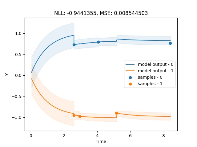
In this section, we explicitly study the sample efficiency of NESDE vs. GRU-ODE-Bayes in a problem with no control signal. Specifically, we generate data from the GitHub repository of De Brouwer et al. 2019. The data consists of irregular samples of the two-dimensional Ornstein-Uhlenbeck process, which follows the SDE
where the noise follows a Wiener process, which is set in this experiment to have the covariance matrix
The process is sparsely-observed: we use a sample rate of (approximately observations for 10 time units). Each sampled trajectory has a time support of 10 time units. The process has two dimensions, and each observation can include either of the dimensions or both of them. The dynamics of the process are linear and remain constant for all the trajectories; however, the stable “center” of the dynamics of each trajectory (similarly to in Eq. 6) is sampled from a uniform distribution, increasing the difficulty of the task and requiring to infer in an online manner.
Fig. 11 presents a sample of trajectory observations along with the corresponding predictions of the NESDE model (trained over 400 trajectories). Similarly to De Brouwer et al. 2019, the models are tested over each trajectory by observing all the measurements from times , and then predicting the process at the times of the remaining observations until the end of the trajectory.

To test for data efficiency, we train both models over training datasets with different numbers of trajectories. As shown in Fig. 12, the sparsely-observable setting with limited training data causes GRU-ODE-Bayes to falter, whereas NESDE learns robustly in this scenario. The advantage of NESDE over GRU-ODE-Bayes increases when learning from smaller datasets (Fig. 12, top), or when predicting for longer horizons (Fig. 12, bottom). This demonstrates the stability and data efficiency of the piecewise linear dynamics model of NESDE in comparison to non-linear ODE models.
Appendix F Medication Dosing Prediction: Implementation Details
Below, we elaborate on the implementation details of Section 6.
F.1 Data preprocessing
Heparin: We derive our data from the MIMIC-IV dataset [Johnson et al. 2020], available under the PhysioNet Credentialed Health Data License. For the UH dosing dataset, we extract the patients that were given UH during their intensive care unit (ICU) stay. We exclude patients that were treated with discrete (not continuous) doses of UH, or with other anticoagulants; or that were tested for aPTT less than two times. The control signal (UH dosing rate) is normalized by the patient weight. Each trajectory of measurements is set to begin one hour before the first UH dose, and is split in the case of 48 hours without UH admission. This process resulted with trajectories, containing a continuous UH signal, an irregularly-observed aPTT signal, and discretized context features. Note that we do not normalize the aPTT values.
Vancomycin: The VM dosing dataset derived similarly, from patients who received VM during their ICU stay, where we consider only patients with at least VM concentration measurements. Each trajectory begins at the patient’s admission time, and we also split in the case of 48 hours without VM dosage. Additionally, we add an artificial observation of at time , as the VM concentration is before any dose was given (we do not use these observations when computing the error).
General implementation details: For each train trajectory, we only sample some of the observations, to enforce longer and different prediction horizons, which was found to aid the training robustness. Hyperparameters (e.g., learning rate) were chosen by trial-and-error with respect to the validation-set (separately for each model).
Context variables are used in both domains. We extract features, some measured continuously (e.g., heart rate, blood pressure), some discrete (e.g., lab tests, weight) and some static (e.g., age, background diagnoses). Each feature is averaged (after removing outliers) over a fixed time-interval of four hours, and then normalized.
F.2 LSTM Baseline Implementation
The LSTM module we use as a baseline has been tailored specifically to the setting:
- 1.
It includes an embedding unit for the context, which is updated whenever a context is observed, and an embedded context is stored for future use.
- 2.
The inputs for the module include the embedded context, the previous observations, the control signal and the time difference between the current time and the next prediction time.
- 3.
Where the control signal is piecewise constant: any time it changes we produce predictions (even though no sample is observed) that are then used as an input for the model, to model the effect of the UH more accurately.
We train it with the same methodology we use for NESDE where the training hyperparameters chosen by the best performance over the validation data.
Architecture for the medication dosing benchmarks: The model contains two fully connected elements: one for the context, with two hidden layers of size and -dimensional output which is fed into a activation; the second one uses the LSTM output to produce a one-dimensional output, which is fed into a ReLU activation to produce positive outputs, its size determined by the LSTM dimensions. The LSTM itself has an input of dimensions; for the context, control, previous observations and the time interval to predict. It has a hidden size of and two recurrent layers, with dropout of . All the interconnections between the linear layers include ReLU activations.
Architecture for the synthetic data benchmarks: Here, there is no context, then the model contains one fully connected element that receives the LSTM output and has two linear layers of sizes and with a Tanh activation between them. The LSTM has an input of dimensions; for the state, control signal, and the time interval to predict. It has a hidden size of and two recurrent layers, with dropout of .