Magnitude-squared coherence: A powerful tool for disentangling Doppler planet discoveries from stellar activityJournal: AJFacilities: Keck (HIRES), ESO La Silla 3.6m (HARPS), Telescopio Nazionale Galileo (HARPS-N)NWelch (Dodson-Robinson 2022),
FINUFFT (Barnett et al. 2019; Barnett 2021),
astropy (Astropy Collaboration et al. 2013),
redfit-x (Ólafsdóttir et al. 2016)
Abstract
If Doppler searches for earth-mass, habitable planets are to succeed, observers must be able to identify and model out stellar activity signals. Here we demonstrate how to diagnose activity signals by calculating the magnitude-squared coherence between an activity indicator time series and the radial velocity (RV) time series . Since planets only cause modulation in RV, not in activity indicators, a high value of indicates that the signal at frequency has a stellar origin. We use Welch’s method to measure coherence between activity indicators and RVs in archival observations of GJ 581, Cen B, and GJ 3998. High RV-H coherence at the frequency of GJ 3998 b, and high RV-S index coherence at the frequency of GJ 3998 c, indicate that the planets may actually be stellar signals. We also replicate previous results showing that GJ 581 d and g are rotation harmonics and demonstrate that Cen B has activity signals that are not associated with rotation. Welch’s power spectrum estimates have cleaner spectral windows than Lomb-Scargle periodograms, improving our ability to estimate rotation periods. We find that the rotation period of GJ 581 is 132 days, with no evidence of differential rotation. Welch’s method may yield unacceptably large bias for datasets with observations and works best on datasets with . Tapering the time-domain data can reduce the bias of the Welch’s power spectrum estimator, but observers should not apply tapers to datasets with extremely uneven observing cadence. A software package for calculating magnitude-squared coherence and Welch’s power spectrum estimates is available on github.
Keywords:
Time series analysis (1916), Period search (1955), Astrostatistics techniques (1886), Radial velocity (1332), Stellar activity (1580), Stellar rotation (1629)I Introduction
Planets are often diagnosed in radial velocity (RV) periodograms as large peaks which register above some high significance level. While some periodogram peaks genuinely describe planets, others are spurious detections resulting from stellar rotation or activity (Saar & Donahue 1997; Hatzes 2002; Desort et al. 2007; Boisse et al. 2011; Robertson & Mahadevan 2014; Robertson et al. 2014; Newton et al. 2016; Suárez Mascareño et al. 2017; Rajpaul et al. 2021, e.g.). Now that extreme precision spectrographs are on the hunt for terrestrial planets (Jurgenson et al. 2016; González Hernández et al. 2018; Gupta et al. 2021), the need for high-performance activity diagnostics is urgent: while an earthlike planet orbiting a sunlike star yields an RV oscillation with semiamplitude cm s-1, that same star’s expected rotational RV modulation has amplitude m s-1 (Vanderburg et al. 2016). Doppler surveys won’t yield any Earth analogs unless stellar signals can be accurately identified and modeled.
A sure sign that a peak in the RV periodogram is caused by stellar activity is when the periodogram of a simultaneously measured activity indicator such as H, Mt. Wilson S-index, or bisector span shows the same peak (or its harmonic) (Queloz et al. 2001; Bonfils et al. 2007; Kane et al. 2016; Sarkis et al. 2018; Toledo-Padrón et al. 2019, e.g.). However, for quiet target stars with low-level variability, the signal in the activity-indicator power spectrum might not hit a statistically significant false alarm probability. In such cases, the connection between stellar activity and RV might be overlooked (Robertson et al. 2015; Bortle et al. 2021; Lubin et al. 2021, e.g.). Furthermore, aliasing, small sample size, and red noise can cause bootstrap false alarm level calculations to fail (Baluev 2008; Chernick 2008; Littlefair et al. 2016), making it difficult to correctly assess the significance of activity signals. Another common diagnostic of stellar activity—a linear regression of RV onto an activity indicator (Queloz et al. 2001; Huélamo et al. 2008; Queloz et al. 2009; Tal-Or et al. 2018, e.g.)—fails when the RV and activity signals are not in phase, as seen in the RV, S-index, and H-index measurements of 55 Cnc (Butler et al. 2017; Bourrier et al. 2018). To validate planet discoveries, we require analysis techniques that reveal all oscillatory components common to simultaneous time series, regardless of relative phase.
In this paper, we demonstrate the use of the magnitude-squared coherence in RV planet searches. This bivariate statistic diagnoses oscillations that manifest in more than one observable. Magnitude-squared coherence can be interpreted as a frequency-dependent correlation coefficient that describes the proportion of variance in one time series that can be explained by means of a lagged linear regression onto another time series. For example, if RV and and (Noyes et al. 1984) both oscillate at the star rotation frequency—as happened when Cen B had a large spot group in 2010 (Dumusque et al. 2012; Thompson et al. 2017)—the coherence would be high at that frequency, and it would be possible to predict RV using a lagged regression onto if the observations were regularly spaced in time (Shumway & Stoffer 2001). Bivariate statistics are used in a myriad of physical science applications, such as solar physics (Walker & Stephenson 2014), climatology (Thomson 1995), oceanography (Chave et al. 1992; Miller & Kelley 2021), atmospheric science (Krug et al. 2019), seismology (Scafetta & Mazzarella 2015), and others (Carter 1987).
This paper is organized as follows. In §II, we present the mathematical fundamentals of the magnitude-squared coherence and its two companion bivariate statistics, the cross-spectrum and phase spectrum. In §III, we describe computational methods used to estimate . In §IV, we demonstrate our methods’ stellar activity diagnostic power using published RV observations of Cen B, GJ 581, and GJ 3998. We present our conclusions and plans for future work in §V. Appendix A introduces our new publicly available software package, NWelch (Dodson-Robinson 2022), which was used for all calculations involving real RV data that are presented here.
| Symbol | Definition |
|---|---|
| time stamp | |
| time between observations | |
| , | time series |
| number of data points in time series | |
| expected value of series | |
| sample mean of series | |
| expected value | |
| cross-correlation between series and | |
| sample cross-correlation between series and | |
| time lag (independent variable in cross-correlation) | |
| (Nonuniform) Fourier transform | |
| cross-spectrum of time series and | |
| estimated cross-spectrum of time series and | |
| estimated cospectrum between time series and | |
| estimated quadrature spectrum between time series and | |
| estimated magnitude-squared coherence between and | |
| , | estimated power spectra of time series and |
| estimated relative phase spectrum of and | |
| convolution | |
| estimated value of | |
| variance | |
| Fisher’s variance-stabilizing transformation of | |
| taper coefficients | |
| spectral window | |
| number of segments used in Welch’s algorithm | |
| effective number of independent estimates , , | |
| , , | observations and taper coefficients belonging to segment |
| , , | , , estimated using , taken from segment |
| , , | tapered estimates of , |
| number of data points in segment | |
| Rayleigh resolution of | |
| approximate bias of magnitude-squared coherence estimator | |
| debiased magnitude-squared coherence estimate | |
| FAL | false-alarm level |
| false-alarm probability | |
| half-width of the main lobe of the spectral window | |
| maximum value | |
| threshold periodogram power for Fisher’s test | |
| threshold periodogram power for Siegel’s test | |
| number of entries in the frequency grid | |
| proportionality constant relating and | |
| Siegel’s test statistic |
II Mathematical fundamentals of magnitude-squared coherence
Suppose a planet-search team is lucky enough to have an extreme-precision spectrograph in space. There are no equipment problems that require telescope downtime, and all data downlinks can be completed in under 24 hours. The team has the luxury of observing a sunlike target at the same time every Earth day, with no interruptions, for many years. The resulting observations are evenly spaced, with constant day (where is a time stamp and is an integer index; symbol definitions are collected in Table 1). From each astronomical spectrum, the data pipeline returns RV plus dozens of activity indicators (Wise et al. 2018, e.g.). The team has assembled the perfect multivariate planet-search time series, which should allow members to characterize all stellar signals.
Knowing that any signal manifesting in both an activity indicator and RV time series cannot be driven by an earthlike planet (Shkolnik et al. 2003, after all, exo-Earths are too miniscule and too far from their host stars for tides to trigger stellar activity as in HD 179949;), the team decides to use the cross-correlation as an activity diagnostic. The cross-correlation between two jointly stationary time series and is defined as
| (1) |
where denotes expected value, , , and is an integer time lag. When observed at contiguous time points , can be estimated using the convolution formula (Shumway & Stoffer 2001, Equations (1.29), (1.40))
| (2) |
where is the sample mean of the series , is the sample mean of the series , and denotes an estimate of . Oscillations with period that manifest in both and will yield local maxima in at integer multiples of and local minima where the lag is such that the oscillation is perfectly out of phase, generating a wave pattern that is easy to see in a plot. The top panel of Figure 1 shows two synthetic regularly spaced time series with representing possible spacecraft measurements. Let denote a noisy activity indicator time series that records the star rotation with period days, while is the noisy RV time series that shows both the rotation and a planet with period days:
| (3) | ||||
| (4) |
where is the rotation frequency, is the planet frequency, and and denote uncorrelated Gaussian white noise processes with zero mean and unit variance. The middle panel of Figure 1, which shows as a function of , demonstrates that there is no zero-lag, straight-line relationship between the two observables because of both the phase shift in the shared rotation signal and the noise in each time series. But the shared oscillation is obvious in the bottom panel of Figure 1, which reveals a wave pattern with period in .

If the real data are noisier than our synthetic and or the two time series share more than one oscillation—such as rotation and a long-term activity cycle—it is more difficult to identify the periods of shared signals in a plot of . To pinpoint the frequencies of oscillations in common to both and , the planet-search team can estimate the (complex valued) frequency-dependent cross-correlation, or cross-spectrum, using
| (5) | ||||
| (6) |
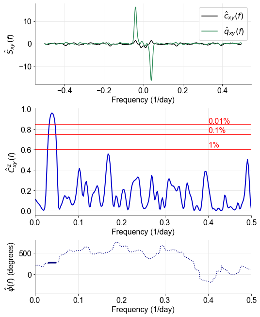
where is the frequency. In-phase and out-of-phase sinusoids that occur in both and yield delta functions in (the cospectrum)11 1 Actually the signals that appear in the cross-spectrum will be shaped by the spectral window (§III.3), but for this “perfect dataset” example they will approximate delta functions in the limit as ., while phase-shifted oscillations in common to and show up as delta functions in (the quadrature spectrum). In general, the cospectrum—an even function—is large when there is a small phase angle near zero, and the quadrature spectrum—an odd function—is large and positive when there is a phase angle near , and will be negative when the phase separation approaches 270∘. Coherent oscillations with relative phases that are not integer multiples of will yield delta functions in both the cospectrum and the quadrature spectrum. Where and share multiple oscillations, the cross-spectrum will have delta functions at all oscillation frequencies. The top panel of Figure 2 shows for our synthetic spacecraft dataset. The shared but phase-shifted rotation signal creates spikes in the quadrature spectrum at days-1.
One can normalize to produce the frequency-dependent cross-correlation coefficient, or magnitude squared coherence
| (7) | ||||
| (8) |
To compute power spectrum estimates and , replace the in Equation 6 with or . In Equation 8, and are normalization factors that control for the fact that different observables might have vastly different amplitude variations—for example, RV semiamplitudes are of order unity or larger even for quiet sunlike stars (Vanderburg et al. 2016), while the H index defined by Gomes da Silva et al. 2011 records oscillations at the 1% level (Robertson et al. 2015, e.g.). If and are activity indicator and RV, respectively, should be near zero at the orbital frequency of any planet candidate. As approaches unity, it lends more support to the hypothesis that the velocity signal at is caused by stellar activity. The estimated phase spectrum, or frequency-dependent phase lag between the two time series, is
| (9) |
is especially useful at frequencies where exceeds some threshold of statistical significance. The middle panel of Figure 2 shows the estimated magnitude-squared coherence between our example and , while the bottom panel shows the estimated phase spectrum . The shared rotation signal shows up in as a strong peak at , while the planet signal at that appears only in RV does not show up in at all. This example shows the power of magnitude-squared coherence in separating activity signals from planets.22 2 For our synthetic dataset, and were computed in python 3 with scipy.signal.csd and scipy.signal.coherence, respectively. To estimate , each time series was divided into six overlapping segments and a Blackman-Harris taper was applied to each segment. See §§III.1 and III.3 for more on segmenting and tapering the time series.
Of course, we do not have an extreme-precision spectrograph on a spacecraft with no-fail instrumentation and rapid downlink. Like all ground-based astronomical time series, RV and activity-indicator datasets are sampled at uneven intervals, with daytime and seasonal gaps. When the time between spectroscopic observations is not constant, no direct cross-correlation estimate can be calculated. But with a non-uniform fast Fourier transform algorithm, it is still possible to estimate the cross-spectrum between RV and an activity indicator (Scargle 1989). Define the nonuniform fast Fourier transform (NFFT) of the sequence observed on the sequence of times where implicitly as
| (10) |
where is the index of the frequency grid and has been standardized to the scaled time interval . That is, to solve for the coefficients one computes , the adjoint of the matrix with entries (Keiner et al. 2009), and multiplies by the column vector of observations (Springford et al. 2020). (See §A.2 for more on the NFFT algorithm.) In what follows, we use the notation to denote the NFFT on a grid of equally spaced Fourier frequencies . When the data are equally spaced in the time domain, the inverse transform can be easily written in closed form. Replacing the Fourier transform with NFFTs, one can obtain the following (normalized) power spectral density estimator
| (11) |
and similarly, an estimator for the cross spectrum
| (12) |
(where deontes complex conjugate), which has the desired property that convolution of the sequences and results in the multiplication of their Fourier transforms, i.e. . For a description of the NFFT algorithm, see §A.2.
Equation 12 reveals a trap for the unwary: if the magnitude-squared coherence is calculated based only on a single estimate of each of , , and , the disastrous result will be . To see why, we substitute Equation 12 into Equation 8: the result is . But if we have estimates of , say for , we can take advantage of the fact that
| (13) |
Thus a meaningful coherence estimate comes from averaging together multiple estimates of the numerator and denominator of Equation 8 before computing their ratio:
| (14) |
The question becomes, how do we obtain the ? For RV datasets, we will divide each time series into shorter segments and compute one estimate of each of , , and from each segment (§III.1). The signal processing literature describes this procedure as Welch’s method.
For bivariate frequency-domain analysis, there is one more useful mathematical operation. As mentioned above, is bounded between 0 and 1, which means is a function of (where denotes variance). In practical terms, this means the difference between (for example) and might be more statistically significant than the difference between and (depending on and ). To stabilize and remove some of its dependence on , we can use Fisher’s transformation (Fisher 1929; Jenkins & Watts 1968):
| (15) |
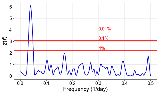
where is the inverse hyperbolic arctangent. The transformed coherence is approximately Student distributed (Thomson & Chave 1991). Figure 3 shows from the estimate plotted in Figure 2.
In the next section, we describe the computational methods used to estimate , , and for RV data.
III Computational methods
The biggest challenge in applying Equation 14 is obtaining multiple estimates of . For evenly spaced data (constant ), there are three possibilities: the multitaper method of Thomson 1982, where the time-domain data are multiplied by a set of orthogonal sequences (Slepian 1978) and the results from subsequent Fourier analysis are averaged together via jackknife mean (Thomson 1995, see a bivariate application of this technique in), smoothing the cross spectrum across frequency (Shumway & Stoffer 2001), or Welch’s method (Welch 1967).33 3 A forthcoming paper will extend multitaper analysis to RV data (Dodson-Robinson et al. in preparation). That paper will build on the work of Springford et al. 2020, who applied the multitaper technique to Kepler data with near-constant . Here we demonstrate how to apply the computationally lightweight Welch’s method to RV data. Our methods borrow heavily from the software package redfit-x (Ólafsdóttir et al. 2016) and its predecessor SPECTRUM (Schulz & Stattegger 1997), which implement Welch’s method for analysis of unevenly spaced, bivariate paleoclimate data.
III.1 Segmenting the data
Welch 1967 built on the work of Bartlett 1948, who proposed estimating the power spectrum of a stationary, regularly spaced time series by dividing the series into segments, computing a periodogram of each segment, and averaging the periodograms:
| (16) |
where is the number of segments and denotes the NFFT of the data subsequence of length .44 4 In Welch’s original work on regularly spaced time series, is the fast Fourier transform and for all . For bivariate time series observed at the same time stamps , one uses the same segmentation scheme for both and (i.e. two observables measured from the same astronomical spectrum taken at time are assigned to the same segment ) and computes , , and for each segment. Averaging together the different estimates of the cross-spectrum and power spectra yields , , and —all the ingredients needed to compute using Equation 14. Figure 4 shows the Dumusque et al. 2012 Cen B time series divided into non-overlapping segments in preparation for using Equation 16.

Bartlett 1948 and Welch 1967 explored time-series segmenting not because they wanted to compute magnitude-squared coherences, but because they were looking for a power spectrum estimator whose variance decreases as the number of observations increases. This is not true of either the standard periodogram (Schuster 1898) or the Lomb-Scargle periodogram (Lomb 1976; Scargle 1982): for both estimators, the variance is independent of the number of observations. Welch 1967 pointed out that non-overlapping segments (aka Bartlett’s method) are ideal for reducing the variance of any , as the various are fully independent of one another. But there is a catch. Although both the standard periodogram and the Lomb-Scargle periodogram are asymptotically unbiased—i.e. as —the bias can be severe for small or even not-so-small (Percival 1994, “tragedy of the periodogram,”). To understand bias, suppose an RV time series traces a planet in a circular orbit with period . Since the planet’s time domain signature is a perfect sinusoid, should have an infinitely thin delta function at . But the finite duration of creates spectral leakage: in , the planet’s signal will land mostly on the frequency nearest to , but there will be non-zero contributions to every frequency in the grid (Harris 1978, e.g.). This leakage is responsible for periodogram bias. Thus there is a tradeoff between bias and variance: we want a large number of segments in order to improve the consistency of , , and , but if is too low our power spectrum and coherence estimates will be consistently biased—that is, will be far away from —especially at high frequencies (Podesta 2006; Bronez 1992; Percival & Walden 2020, e.g.).
III.2 Overlapping segments
To reduce the bias of each while retaining most of the variance suppression associated with large , Welch 1967 proposed using tapered, overlapping segments (tapering is discussed in §III.3). In the 50% overlap scheme, we segment as follows:
Each 50% overlapping segment has data points, as opposed to for non-overlapping segments. But because of the overlap, the resulting spectral estimates are not independent. The variance reduction associated with overlapping segments is
| (17) |
where is an effective number of segments. The left panel of Figure 5 depicts the allocation of data points in a sample among segments in Welch’s 50% overlapping segment method.
 |
 |
III.3 Tapering
The value of depends on the type of taper (also called a window) applied to each segment. Tapers are functions that are pre-multiplied with and to minimize spectral leakage, and are especially valuable for detecting weak signals in the neighborhood of much stronger signals. They are normalized such that so as to conserve power. Figure 6 shows a synthetic RV dataset from a star with two unequal-mass planets in circular orbits:
| (18) |
where days-1 and days-1.55 5 From a dynamical perspective, such a planetary system is unlikely to be stable; we use it here merely for illustrative purposes. When no taper is applied (i.e. the dataset retains its rectangular or “boxcar” taper associated with the fact before and after the observing run such that ), one does not detect the signal associated with planet 2 in . But when a minimum 4-term Blackman-Harris taper (Harris 1978, equation 33 of) is applied to , so that the power spectrum estimate becomes
| (19) |
planet 2 is detected despite being responsible for only 0.028% of . Here is not computed with Welch’s algorithm—it is a standard Schuster 1898 periodogram. See §A.1 for reasons why Figure 6 and all subsequent power spectrum plots have logarithmic y-axes.
 |
 |
Viewing tapering from a frequency domain context, when the time series is evenly spaced with , we have the following (Percival & Walden 2020, p. 186):
| (20) |
which is a convolution between the true power spectrum and the spectral window , defined as
| (21) |
That is, the bias of the power spectrum estimator comes from convolving the true power spectrum with the spectral window. Since spectral leakage is created by the “smearing” effect of the Fourier transform of the spectral window, it’s best if resembles a delta function as closely as possible (Harris 1978). For RV datasets, we calculate using the adjoint NFFT by replacing with in Equation 10. Note that when generalizing Equation 20 to unevenly spaced time series, one does not strictly obtain a convolution between and , since in general the NFFT cannot simply be inverted (Scargle 1982, Appendix D). However, we will see in §IV that peaks in the RV power spectra are shaped like , and will follow Scargle 1982 in referring as the “spectral window.”
When applying Welch’s algorithm, tapering the overlapping segments not only mitigates spectral leakage—it also increases the independence of the various . To see why, we examine the right panel of Figure 5, which shows tapers applied to each segment depicted in the left panel of Figure 5. At data point , where is highest, is nearly zero. Where is at its maximum, overlapping tapers and are near zero, and so on. The tapers ensure that very little information contained in segment gets repeated in segments or . The effective number of segments is
| (22) |
where is a constant that depends on the type of taper applied (Welch 1967). The boxcar taper belonging to otherwise untapered segments has , while the minimum 4-term Blackman-Harris taper has , yielding . Figure 7 shows the GJ 3998 RV data of Affer et al. 2016 broken into two 50%-overlapping segments with the associated minimum 4-term Blackman-Harris tapers.

If all RV planet-search data were observed at evenly spaced time intervals, as in the spacecraft example in §II, the benefits of applying tapers to the Welch’s segments when computing , and would far outweigh the drawbacks.66 6 The high dynamic range delivered by the minimum 4-term Blackman-Harris taper and other similar spectral windows comes at the cost of some resolution in the frequency domain; see §III.6 for more on how tapering affects resolution. Re-examining Figure 6, we see that —the tapered power spectrum estimate of from Equation 18—has a dynamic range of over 13 orders of magnitude. This dynamic range would allow planet hunters to identify terrestrial planets, hot Jupiters, rotation, and activity cycles all in the same RV power spectrum estimate : there would be no need to fit the strongest signal, subtract it out, examine a periodogram of the residuals, and keep iterating until no more signals were found. When the temporal cadence is only mildly uneven—as is common in paleoclimatology—the Blackman-Harris window and other similar tapers retain most of their bias-suppression ability (Ólafsdóttir et al. 2016, e.g.).
But the wildly uneven observing cadence of RV time series often destroys the tapers (Scargle 1989, e.g.). Figure 8 shows the effect of tapering the 51 Peg b RV dataset of Butler et al. 2006. The top left shows the published data , while the bottom left shows , where is the minimum 4-term Blackman-Harris taper evaluated at the observation timepoints . The top right shows that the planet’s signal (black dotted line) is clearly visible in (blue dash-dot line), while on the bottom right, shows nothing but noise. Almost all of the 51 Peg observations took place at the very beginning and the very end of , when the interpolated is near zero, so tapering removes nearly all the information contained in the time series. When the observing cadence is extremely uneven, we revert to the boxcar tapers when computing . A good rule of thumb is that all tapers should retain the bell-like shapes shown in the right panel of Figure 5. If the ‘‘bell’’ is missing huge chunks or its shape is not recognizable when plotted, tapering may do more harm than good.77 7 Not all useful tapers have bell shapes in the time domain—in particular, higher-order multitapers have zero crossings (Slepian 1978; Thomson 1982)—but in this work we use only bell-shaped tapers.

III.4 Gaps, weighting, and number of data points per segment
Another consideration when applying Welch’s algorithm to RV data is that large gaps in the middle of a segment should be avoided when possible. Gappy segments are difficult to handle because the resolution limit of , , and is set by the time duration of the segments:
| (23) |
where is the final timestamp in segment , is the first timestamp in segment , and —called the Rayleigh resolution in analogy to Rayleigh’s criterion in optics—is both the smallest oscillation frequency that can be detected and the frequency separation of two barely resolved peaks (Godin 1972, e.g.). For evenly spaced data, is the same for all segments, but RV datasets always yield varying . A segment that contains one or more large gaps has a low apparent Rayleigh resolution, which makes one optimistic that low-frequency information missing from other segments might be available in . But is often misleading at small integer multiples of because the gaps make for poor phase coverage of low-frequency oscillations. Here we use the segment with the longest time duration88 8 The longest-duration segment does not necessarily have the highest number of data points ; it is simply the segment with the largest value of (Equation 23). to define the Rayleigh resolution of , , , and , but we urge caution when examining the low-frequency end of each statistic if one or more segments contains a large gap.
In practice it is difficult to keep the Welch’s segments gap-free, as seasons and telescope scheduling often combine to isolate a handful of data points from the rest of the time series. The Cen B time series of Dumusque et al. 2012 shown in Figure 4 would ideally be broken into four segments, but we use only three segments because the first observing season (modified Julian dates 54550–54650) recorded just 42 observations—not enough to yield a low-bias periodogram (Pukkila & Nyquist 1985; Springford et al. 2020). No tapers are applied to the Cen B data because of the gap in segment 1. With non-overlapping, boxcar-tapered segments, the Cen B segmenting scheme differs from Bartlett’s method only in that each segment has a different number of data points. For all segmenting patterns, the average cross-spectrum is weighted by the number of data points in each segment:
| (24) |
Average periodograms and are likewise weighted by .
To mitigate the worst manifestations of small-sample bias, we recommend that all segments have (Hannan & Nicholls 1977; Pukkila & Nyquist 1985), which requires for 50% overlapping segments. But many published RV datasets have fewer than 100 observations (a practice we do not endorse). Based on the simulations of Das et al. 2021, who generated small-sample realizations of AR and ARMA processes and compared the resulting periodograms with the processes’ analytically known power spectra, we consider a hard lower limit. This means the minimum number of astronomical observations required for Welch’s algorithm is 75 (two 50%-overlapping segments each with ), though more is much better. (In fact, Thomson & Haley 2014 present a time series with for which the periodogram, which records a power-law turbulent cascade, is still biased by more than seven orders of magnitude.) The transformed coherence and its noise properties can only be described analytically by Gaussian statistics when (Enochson & Goodman 1965; Jenkins & Watts 1968), which requires . With small , the false positive risk may depart from theoretical expectations in unpredictable ways (see below).
III.5 Bias correction and false alarm levels
While minimizing bias in , , and is always an important consideration when deploying Welch’s algorithm, an approximate bias correction to is possible. The bias on the magnitude-squared coherence measurement is
| (25) |
(Carter et al. 1973; Bendat & Piersol 2010). The debiased coherence estimate is therefore
| (26) |
All analyses of RV data presented in §IV use debiased coherence estimates.
One can also calculate analytical false alarm levels (FALs) for :
| (27) |
(Carter 1977; Schulz & Stattegger 1997), where FAL is the threshold associated with false-alarm probability . Equation 27 gives false alarm thresholds for given true coherence , i.e. the two time series trace completely unrelated physical phenomena. If a broad-spectrum random process (such as granulation) manifests in both and , then Equation 27 gives artificially low FALs for periodic signals because the two time series have some underlying non-zero coherence at all frequencies. The NWelch software package has an option for calculating frequency-dependent bootstrap FALs for in addition to using Equation 27. All FALs presented here are calculated using 10,000 bootstrap iterations.
III.6 Resolution and the spectral window
While the Rayleigh resolution (Equation 23) is the theoretical frequency separation between two barely resolved peaks in , , or , the true frequency resolution of each statistic is determined by the width of the main lobe in the spectral window . Resolution therefore depends on the choice of taper. In Figure 6, we see that the power spectrum peak associated with planet 1 is quite narrow when the boxcar taper is retained. Although the boxcar taper has poor statistical properties when it comes to leakage and bias, it works well for separating closely spaced signals of similar power. Thus boxcar tapers are useful for asteroseismologists who are trying to resolve modes separated by the small spacing, though they are not optimal for planet hunters who might have to deal with signals of widely varying power. The planet hunter’s penalty for using a taper to increase the dynamic range of is lower resolution in all . Following Harris 1978, we quantify the half-width of the main lobe in as the frequency interval over which a sinusoidal signal declines from its peak value by 6 deciBels (dB), or a factor of . One resolution unit is wide.
Harris 1978 calculated as a function of for a variety of tapers applied to evenly spaced time series. For the boxcar taper, .99 9 Astronomy students may find 1.21 an easy constant to remember, as it’s quite similar to the constant in the telescopic Rayleigh resolution equation for a circular aperture, (where is the telescope resolution limit, is the observation wavelength, and is the telescope diameter). The minimum 4-term Blackman-Harris taper has , while the Kaiser-Bessel window (another taper option available in NWelch; see §A) has . The fact that is a function of means harmonic analysis has a resolution-variance tradeoff in addition to the bias-variance tradeoff discussed in §III.1. Users of Welch’s method can either prioritize high resolution by constructing a small number of long-duration segments, or emphasize false positive suppression by deploying a larger number of shorter-duration segments. (Of course, small samples and seasonal gaps can constrain the segmenting scheme, making it difficult to find an optimal balance between resolution and variance.) Since almost all RV datasets require segments of varying duration (e.g. Figure 4), we estimate the main lobe half-width of the Welch’s estimator as the mean of the main lobe half-widths from the individual segments, weighted by number of points per segment:
| (28) |
where is defined in Equation 23.
In practice, the Welch’s estimator for unevenly spaced datasets has spectral resolution that depends on the exact timing of the observations, not just the segment durations. (The dependence on observation timing applies to the main-lobe width of the Lomb-Scargle spectral window as well.) It is therefore possible for the actual resolution unit to differ from given by Equation 28. NWelch allows the user to examine the specific associated with any Welch’s segmenting and tapering scheme. The software will then empirically calculate by finding the frequency at which , where is the maximum value.
We recommend examining not just to find the resolution of a given Welch’s estimator, but because changing the segmenting scheme can strongly alter the shape of the spectral window. For example, Figure 9 compares from the Lomb-Scargle periodogram and the 3-segment Welch’s estimator applied to the Dumusque et al. 2012 Cen B dataset (Figure 4). As we know from §III.3, a periodic signal does not yield a delta function in —it instead creates a copy of centered at the signal frequency. Since the Lomb-Scargle spectral window is beset by “ringing,” there can be no clean, isolated peaks in the Lomb-Scargle periodograms of RVs and activity indicators, as noted by Rajpaul et al. 2016. The Welch’s spectral window, which has a well-defined main lobe, is much better suited to identifying periodic signals. Figure 9 suggests that spectral window optimization using Welch’s method will be a productive avenue for future research.

III.7 Siegel’s test
The last computational method we will describe applies only to power spectrum estimates, not to magnitude-squared coherences, but it is useful for deciding whether a dataset contains periodic signals or just noise. Planet hunters often struggle with unrealistic-looking bootstrap false alarm levels (see §2.2 of Cumming 2004 for information on how to calculate bootstrap FALs). For example, the top left panel of Figure 10 shows the H-index time series measured by Robertson et al. 2015 from the Kapteyn’s star spectroscopic dataset of Anglada-Escude et al. 2014. The time series yields a Lomb-Scargle periodogram with signals that exceed the bootstrap 1% FAL (Figure 10, top right; periodogram computed with NWelch). But should we really believe that a time series with only 112 measurements can record 10 distinct oscillations? It’s more likely that the FALS are misleading (Robertson et al. 2015, indeed, the same false-alarm threshold problem can be seen in the Lomb-Scargle periodogram of the same dataset in Figure 1 of), with small-sample statistics, spectral leakage, and aliasing all contributing to the bootstrap failure (Chernick 2008, e.g.). The spectral window shown in the bottom panel of Figure 10 has a broad main lobe and a large number of spurious spikes, suggesting that periodogram peaks are window function artifacts.
 |
 |
 | |
In situations like this, we can deploy Siegel’s test for compound periodicity. Siegel 1980 developed an extension of Fisher’s test, which rejects the null hypothesis of white noise when the maximum power in the normalized periodogram exceeds the critical value . Percival & Walden 2020 approximate as
| (29) |
where is the number of entries in the frequency grid and is the false alarm risk (e.g. for 5% FAP). While Anderson 1971 notes that Fisher’s test is the most powerful identifier of simple periodicity (oscillation at one period only), the test won’t work when there are multiple oscillations—such as planet and rotation, rotation and long-term magnetic activity, or rotation with significant power at one or more harmonics. Siegel’s test uses a reduced threshold , where , and sums all periodogram power in excess of to compute the test statistic :
| (30) |
The value of is then compared with a threshold that depends on the number of entries in the frequency grid. If exceeds the threshold, the null hypothesis of white noise is rejected and the time series is considered to be periodic. When , Siegel’s test is conservatively optimized for two periodicities, whereas is sensitive to three or more periodicities but less robust against noise peaks. For the Kapteyn’s star periodogram in Figure 10, Siegel’s test does not reject the null hypothesis of white noise, even with : there is no evidence for periodicity in the time series. We will use Siegel’s test in §IV to see whether the alternative hypothesis of periodicity is supported for certain time series before using those time series to measure rotation periods. Note that Siegel’s test doesn’t differentiate between a smooth power spectrum with a large dynamic range and a power spectrum consisting of white noise plus a single large oscillation—red noise is a failure mode for both bootstrapping and Siegel’s test. We are currently incorporating FALs calculated against a red noise model into NWelch and will discuss these in a future publication.
IV Application to RV data
Here we use archival data to demonstrate the use of magnitude-squared coherence in diagnosing stellar RV signals. We select three test datasets that have concurrent RV and activity-indicator time series with . We begin by showing that GJ 581 has significant H-RV coherence at the frequencies of the stellar signals that were misidentified as planets GJ 581 d and GJ 581 g, and use a Welch’s power spectrum of the H index to show that both signals are rotation harmonics. Next we demonstrate that high-frequency stellar signals appear in the magnitude-squared coherences between RV and activity indicators in the Cen B dataset assembled by Dumusque et al. 2012. We then use coherence between Mt. Wilson S-index, H index, and RV to argue that GJ 3998 b and c may be misdiagnosed stellar activity signals. This section closes with a step-by-step guide to interpreting magnitude-squared coherence measurements.
IV.1 GJ 581
GJ 581 became the third M dwarf known to host a planetary system after Bonfils et al. 2005 used HARPS to discover a Neptune-mass planet with days. Udry et al. 2007 followed up with reports of planets c ( days) and d ( days), both in or near the habitable zone. Mayor et al. 2009 presented another compelling discovery: planet e ( days, ), one of only a handful of super-Earths discovered in multiplanet systems at the time. They also revised the period of planet d to days, arguing that the one-year alias introduced by Earth’s orbit caused some confusion in the Udry et al. 2007 study. Next, Vogt et al. 2010 used Keck HIRES data to add planets f ( days) and habitable-zone dweller g ( days) to the inventory. The six-planet system with three planets in or near the habitable zone became the object of intense climate modeling efforts (Pierrehumbert 2011; Wordsworth et al. 2011; von Bloh et al. 2011; Heng & Vogt 2011, e.g.).
But papers casting doubt on the existence of one or more of the planets began to emerge almost immediately after the report of planets f and g. Anglada-Escudé & Dawson 2010 suggested that planet g was an alias of an eccentricity harmonic of planet d, while Gregory 2011 argued that a Bayesian multiplanet Kepler periodogram could only reliably detect planets b and c. Forveille et al. 2011 questioned the statistical significance of planets f and g after obtaining 121 new HARPS observations. Baluev 2013 demonstrated that planets d, f, and g could be artifacts of red noise with a correlation timescale of 10 days. Finally, Robertson et al. 2014 demonstrated that ‘‘planet’’ d was actually a stellar signal that, when incorrectly modeled in the time domain, created the artifact interpreted as ‘‘planet’’ g. Today the Extrasolar Planets Encyclopedia1010 10 exoplanet.eu states that GJ 581 hosts only three planets: b, c, and e.
Since Robertson et al. 2014 identified signals d and g as rotation artifacts, we will start by measuring the star’s rotation period. Figure 11 shows Welch’s power spectrum estimates of the time series used in the Robertson et al. 2014 analysis: given (top) and given RV (bottom). Both power spectrum estimates were computed using three 50% overlapping segments with the minimum 4-term Blackman-Harris taper applied to each segment. As with the Cen B dataset, the Welch’s estimates have a much cleaner spectral window than the generalized Lomb-Scargle periodograms (Figure 12). Robertson et al. 2014 found a primary peak in the Lomb-Scargle periodogram at days plus a secondary peak at days and attributed the split peak to phase changes in the rotation signal. However, the signals at and are not quite separated by in the generalized Lomb-Scargle periodogram, so cannot be said to be truly distinct. The Welch’s power spectrum estimate shows a strong single peak that exceeds the 0.1% FAL at days ( days-1), which we take to be the true rotation period. There are also significant peaks at the first two rotation harmonics, and . Although spectral window of the Welch’s estimator is wide, the rotation signal and its harmonics are each separated by more than one resolution unit. The Welch’s RV power spectrum has a statistically significant peak at the orbital frequency of planet b ( days-1) plus a local maximum at the frequency of planet c ( days-1), but no obvious signals at the rotation frequency or its harmonics. The conservative Siegel’s test with finds a % chance that both time series are periodic, suggesting that the bootstrap FALs are realistic.


Robertson et al. 2014 used several lines of reasoning to argue that “planets” d and g were really stellar signals: they created a separate fit to RV as a function of for each observing season, identified correlations between and bisector inverse slope, and calculated a new RV model after subtracting off the best-fit seasonal straight-line models RV(). But a single calculation of is enough to reveal the stellar origins of the two signals. Figure 13 shows transformed magnitude-squared coherence given , RV. Gray bands of width are centered at the orbital frequencies of planets b and c. The yellow bands, also of width , are centered at the frequencies of “planets” d and g reported by Vogt et al. 2010. Vertical black dotted lines show rotation harmonics (where is an integer) near which exceeds the 5% FAL. “Planet” d sits right atop the first rotation harmonic () at the center of a resolution unit that includes two statistically significant coherence peaks, one of which exceeds the 1% FAL. “Planet” g is within half a resolution unit of the third rotation harmonic (), which is also the location of a coherence signal that almost reaches the 0.1% FAL. Significant -RV coherence can also be seen at other rotation harmonics: at both and , exceeds the 0.1% FAL. In contrast, the band centered on planet c is clean. The band centered on planet b includes a signal that rises above the 5% FAL. That signal is likely to be a false positive—indeed, we expect to see more than one false positive above the 5% FAL given that our coherence estimate has a frequency range far greater than 20 resolution units—but further study of the GJ 581 system that incorporates other activity indicators might be useful.

The strong signals at the rotation harmonics in Figures 11 and 13 suggest that GJ 581 has a complex rotation signal. Spectral power and coherence at high-order harmonics may result from the star hosting multiple large spots or spot groups (Rodono et al. 1986; Günther et al. 2020; Perger et al. 2021; Perugini et al. 2021, e.g.). In the next section, we will investigate coherent stellar signals that do not appear to be associated with the dominant rotation period, but which may be artifacts of differential rotation, giant cells, or supergranulation.
IV.2 Cen B
The Cen B dataset assembled by Dumusque et al. 2012 has proven to be useful for identifying spectroscopic signatures of stellar activity. While the star is generally quiet (Cincunegui et al. 2007), it developed one or more large spot groups that caused obvious rotational modulation in the time series from 2010 March 23 to 2010 June 12 (Thompson et al. 2017). This modulation is visible in Segment 2 of Figure 4. Wise et al. 2018 used the 2010 March-June data to find activity-sensitive absorption lines with modulation in either half-depth range or core flux, while Thompson et al. 2017 used the same data to identify pseudo-emission features with rotationally driven RV changes. Here we will search for stellar signals using Welch’s power spectra of the activity indicators and magnitude-squared coherence between activity indicators and RV.
Figure 14 shows Welch’s power spectra of full width at half maximum of the cross correlation between the spectrum and a digital mask (FWHM; Pepe et al. 2000, top left), bisector velocity span (BIS; Toner & Gray 1988, top right), (bottom left), and RV (bottom right) calculated using the segmenting scheme in Figure 4. Before applying Welch’s algorithm to the RV data, we removed the binary motion by subtracting the best-fit quadratic model (Endl et al. 2016). To suppress spectral leakage from the long-period activity cycle, each of FWHM, BIS, and and each of RV had a linear trend removed before was calculated. The combination of segmenting and detrending mimics the low-pass filtering applied by Dumusque et al. 2012 and the Gaussian process model constructed by Suárez Mascareño et al. 2017. Figure 14 also shows Lomb-Scargle periodograms in light blue. The Welch and Lomb-Scargle periodograms differ at low partly because the Welch’s estimator contains no information about signals with periods longer than the longest segment duration, and partly because of the detrending.1111 11 See §A for a “like-for-like” comparison between the single-segment, untapered NWelch power spectrum and the astropy.timeseries.LombScargle periodogram.
Although the Welch’s power spectrum of BIS is the only one that has a signal that exceeds the bootstrap white-noise 5% false alarm threshold, Siegel’s test finds that Welch’s power spectrum estimates of all of the activity-indicator time series (FWHM, BIS, ) show periodicity at the 95% significance level (§III.7). We therefore average the frequencies of maximum power in the BIS, FWHM, and periodograms to find the rotation period that best describes the Dumusque et al. 2012 dataset: days ( day-1), which is consistent with rotation period estimates from the literature (DeWarf et al. 2010; Brandenburg et al. 2017; Suárez Mascareño et al. 2017).1212 12 Since rotation signals are quasiperiodic, it’s common for estimates of the rotation period to vary slightly with activity cycle phase and/or number of spot groups on the star surface (Gilbert et al. 2021, e.g.), hence the variety of similar but not identical measurements from the literature. We will use our measured rotation period as a benchmark when searching for stellar signals. Vertical black dotted lines in Figure 14 show shared oscillations identified in the magnitude-squared coherences (see below).

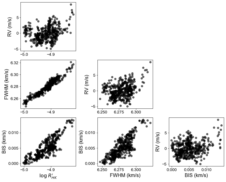
Before we examine any magnitude-squared coherence estimates, we pause to consider Figure 15, which shows scatter plots vs. for all pairs of observables. RV is not well described as a straight-line function of any activity indicator. We can optimistically hope that’s because activity signals are not manifesting in RV, but it’s possible that (a) the relationships between RV and activity indicators are nonlinear, phase-lagged (Figure 1), and/or noisy, or (b) , FWHM, and BIS do not provide a complete description of stellar activity. On the other hand, the activity indicators show obvious straight-line relationships with each other—particularly and FWHM—which suggests that they all trace the same underlying physical processes. In a magnitude-squared coherence analysis with two activity indicators as and , we should expect to see statistically significant values in and .
In Figure 16, we see our prediction of high coherences between the activity indicators borne out. The plots show , the -transformed magnitude-squared coherence, given , FWHM (top); , BIS (middle); and FWHM, BIS (bottom). Solid horizontal lines show false alarm thresholds calculated with Equation 27, while dotted horizontal lines show bootstrap false alarm thresholds (§A). The rotation frequency is marked with a black dash-dot line, with the resolution limit indicated in gray. As expected, all three plots show statistically significant across the entire rotation band. Other frequencies besides rotation at which exceeds the 1% false alarm threshold in at least two of three panels in Figure 16 are marked with vertical yellow dash-dot lines; if a signal at frequency is significant in two of three coherences between activity indicators, it means the oscillation is present in all three indicators. Coherent stellar signals are located at days-1, or days.
We know from Figure 9 that the shared signals are not window function artifacts, but their physical origin is unclear: most of them do not fall at simple rotation harmonics (, where is an integer), though days-1 is within half a resolution unit of the harmonic. Differential rotation sometimes creates secondary peaks in periodograms of photometry and activity indicators (Reinhold et al. 2013); our best guess is that we are seeing a secondary peak, perhaps along with some beating between differential rotation signals. Supergranulation and giant cells may be in play on the shorter timescales (Nordlund et al. 2009). If we re-examine the Welch’s power spectrum estimates of , FWHM, and BIS in Figure 14, we see that the shared signals (again marked by yellow dash-dot lines) are all at or near local maxima. Even though none of those local maxima appear statistically significant when compared with our bootstrap white-noise false alarm thresholds, the underlying oscillations may be real. The downward slopes of for FWHM, BIS, and suggest that false alarm thresholds in the Cen B power spectra should be computed from a red noise model (Ólafsdóttir et al. 2016, e.g.). We are developing this functionality and will include it in a future release of NWelch. Red noise has been incorporated in models of RV data by (e.g.) Baluev 2013, Tuomi et al. 2013, and Feng et al. 2016.

Now we turn to the magnitude-squared coherences between activity indicators and RV. Figure 17 shows given RV and FWHM (top), RV and BIS (middle), and RV and (bottom). The color scheme is the same as in Figure 16. Magnitude-squared coherences in the rotation band are near zero, indicating that no activity indicator is a good tracer of the way rotation manifests throughout the entire duration of the RV dataset. In each panel of Figure 17, signals that exceed the 1% FAL in the estimate shown in that panel only are marked with yellow dash-dot lines. The activity indicators’ shared signal at days-1 (Figure 16) also shows up in coherences between FWHM & RV and & RV. FWHM-RV coherence has a second peak at days-1 ( days, top panel). BIS-RV coherence has peaks at days-1 and days-1 (P = days and days, middle panel). The four coherent RV-activity indicator oscillations are marked in the Welch’s RV power spectrum in Figure 14 (lower-right panel). The FWHM-RV oscillation at days-1 coincides with a local maximum of the Welch’s RV power spectrum. The power spectrum also has a local maximum at days-1, though not the FWHM power spectrum. The coherent RV-BIS oscillation at days-1 is within one resolution unit of peaks in the FWHM and RV power spectra. All four power spectra have a local maximum at days-1.

Our analysis of the Dumusque et al. 2012 Cen B dataset shows that periodic short-timescale stellar activity occurs at other frequencies besides and its harmonics. We have identified seven oscillatory signals that are present in all three activity indicators, plus four coherent activity indicator-RV oscillations. Figure 15 demonstrates that the stellar RV signals could not have been diagnosed by fitting a straight-line model to RV as a function of an activity indicator. Accurately identifying the activity signals is an important step toward suppressing false positives in RV planet searches.
IV.3 GJ 3998
Since 2012, the HArps-N red Dwarf Exoplanet Survey (HADES) program has been surveying 78 early-type M dwarfs for Doppler shifts induced by rocky planets (Perger et al. 2017). The first HADES discovery paper featured two planets orbiting GJ 3998 with periods days and days (Affer et al. 2016). Aware of the tendency of M dwarfs to be more active than solar-type couterparts of the same age, the HADES team examined time series of and Mt. Wilson S-index measured from the same spectra as the RVs, as well as near-simultaneous EXORAP and APACHE photometry. Affer et al. 2016 identified two signals with periods days and days that were present in RV, , and S-index and posited that was the true rotation period while represented modulation due to differential rotation. The photometry was consistent with rotation period . Following Robertson et al. 2014, the HADES team verified that the planetary signals were present in generalized Lomb-Scargle periodograms of RV data from all observing seasons and demonstrated that the Spearman’s rank correlation coefficients of RV as a function of S-index and were insignificant. They then concluded that the signals at and were planetary in origin.
As with GJ 581 and Cen B, we begin our analysis by measuring the star rotation period from Welch’s power spectrum estimates with the segmentation and tapering scheme shown in Figure 7. Affer et al. 2016 explain how the traditional HARPS and HARPS-N way of measuring RVs, by cross-correlating with a mask consisting of a thin rectangle surrounding each spectral line center, is suboptimal for M dwarfs because their spectra feature substantial line blending. Accordingly, in Figure 18 we examine the Welch’s and generalized Lomb-Scargle periodograms from the RV, S-index, and time series measured with the TERRA pipeline (Anglada-Escudé & Butler 2012). The S-index and time series contain statistically significant peaks at 0.0321 days-1 and 0.0311 days-1, respectively, which we average together to find days-1 / days. Our rotation period is similar to identified by Affer et al. 2016. Although the stellar signal with frequency would be more than one resolution unit away from , the Welch’s power spectra do not show any evidence for such a signal.

We now turn to magnitude-squared coherence. Although Affer et al. 2016 emphasize that the TERRA pipeline is preferred over the CCF-based HARPS DRS pipeline for M dwarfs, they nevertheless present RVs measured with both methods. They also present a second set of activity indicator time series, with S-index measured according to Henry et al. 1996 and measured as in Robertson et al. 2013. Accordingly, we analyze coherences with TERRA S-index, H96 S-index, TERRA , and R13 , and with TERRA RV and CCF RV—eight measurements of in all. Figure 19 shows the four transformed coherence measurements with an S-index measurement as . Planets b and c are marked by vertical dash-dot black lines surrounded by a shaded region indicating the resolution unit. In three of four S-RV coherences, there is a peak within half a resolution unit of planet c that exceeds the 1% FAL. The fourth, with H96 S-index and CCF RV, has a signal at that exceeds the 5% FAL. As with GJ 581, we are also seeing high-order rotation harmonics: all estimates have high coherence at the fifth harmonic (), while estimates with CCF RV have high coherence at the third harmonic ().

If we examine the coherences with an measurement as plotted in Figure 20, we find evidence for a stellar signal at the frequency of planet b. When CCF RV, the -RV coherence at exceeds the 0.1% FAL. With the TERRA RVs, we find -RV coherence over the 5% FAL at and nearing the 1% FAL for TERRA . However, the band surrounding planet c is clean. does not have any coherent oscillations with RV directly at the rotation harmonics, though there is a coherence peak almost within a half resolution unit of for TERRA RV. The reason Affer et al. 2016 could not see a straight-line relationship between either and RV or S-index and RV is because there is more than one oscillation shared between RV and the activity indicators—in addition to the planet candidates, rotation harmonics are present, and so are higher-frequency signals that are not obviously associated with rotation, as in the Cen B data.

While we are not yet ready to state definitively that the GJ 3998 RVs show only stellar signals, the system requires further follow-up in light of our results. If coherence between RV and activity indicators at and persists after additional data are taken, that would suggest that the planets are not real. It’s also crucial to measure multiple activity indicators, since they may not all trace the same underlying physical phenomena. Indeed, Robertson et al. 2013 highlight the fact that Ca H&K and H emission come from different chromospheric depths and point out that signal-to-noise ratio is often problematic in the Ca H&K lines in M dwarf spectra.
IV.4 Interpreting magnitude-squared coherence measurements
What should observers look for when applying bivariate frequency-domain techniques to their own planet-search datasets? In our analyses of GJ 581, Cen B, and GJ 3998, we roughly followed the following procedure:
- 1.
Examine the spectral window of the Welch’s estimator. Look for sidelobes that could yield false positives in the power spectra. Calculate the Rayleigh resolution limit, the analytical resolution unit (Harris 1978, e.g.), and the empirical value of for a dataset’s specific observing cadence. NWelch automatically reports these numbers for each segmenting/tapering scheme. Be aware that two signals with a frequency separation of less than are not statistically distinguishable. It’s especially important to consider resolution when searching for planets near the star rotation period or differential rotation.
- 2.
Use Welch’s power spectra of the activity indicators to estimate the rotation period. While many planet-search targets will have previous rotation period measurements in the literature, the quasiperiodic nature of the rotation signal means one might recover a somewhat different rotation period depending on the observational epoch and activity cycle phase (Robertson et al. 2014). It’s important to determine how rotation is manifesting in the particular dataset under analysis. For the Cen B dataset, in which three activity indicators yielded three slightly different rotation period estimates, we averaged together the various estimates (§IV.2). It’s possible that the community will come up with a more sophisticated way to handle differing rotation period measurements.
- 3.
Search for coherence between RV and activity indicators within one resolution unit of the rotation period, the periods of planet candidates, and the harmonics of all of the above. For any planet that is not large enough or close enough to the star to trigger stellar activity, and should be impervious to eccentricity harmonics. Observers who find coherent RV-activity indicator signals at either their planet candidate frequency or its harmonics should use extreme caution before reporting a planet discovery.
It’s unclear how high up the overtone sequence we should expect to see rotation harmonics—for example, if there’s a peak in near the eighth harmonic (), is it truly rotation-related, or is its proximity to a harmonic just a coincidence? We hope stellar physicists will explore the complexity of rotation signals and the extent to which their harmonics should be traceable by RV datasets. We also hope stellar physicists will weigh in on possible sources of coherent RV-activity signals that are not related to rotation.
- 4.
When coherent RV-activity indicator signals are found, check to see whether they line up with local maxima in the power spectra. Sometimes a power spectrum peak that’s not significant when judged against a white noise model indicates a real signal. The signal processing literature features more sophisticated ways of checking the significance of power spectrum peaks, such as F-testing (Thomson 1994, e.g.), false alarm thresholds determined from red noise models (Ólafsdóttir et al. 2016, e.g.), and prewhitening followed by checking against the exponential quantiles. But these techniques are mostly unexplored for RV data. When a peak in corresponds to a local maximum in the RV and/or activity-indicator power spectrum, it lends support to the hypothesis that the coherence is real and not spurious. However, given that the geophysics literature features coherent signals that don’t correspond to power spectrum local maxima (Pardo-Igúzquiza & Rodríguez-Tovar 2012, see example in), one shouldn’t be too quick to dismiss any signals in as false positives.
V Conclusions and Plans for Future Work
Magnitude-squared coherence is a powerful tool for diagnosing stellar signals in bivariate RV-activity indicator time series. By combining Welch’s power spectrum estimates with magnitude-squared coherence measurements, we were able to identify the signals that were originally labeled GJ 581 d, g as rotation harmonics. In the Cen B dataset, we mapped bivariate oscillations onto non rotation-related local maxima in the Welch’s power spectrum estimates of FWHM, BIS, , and RV. Finally, in the GJ 3998 data, we found high coherence between , S-index, and RV at the frequencies of planet candidates b and c. Since it is now standard practice for planet hunters to analyze and publish activity indicator time series along with RVs (Dalba et al. 2021; González-Álvarez et al. 2021; Maldonado et al. 2021, e.g.), and since most stellar signals show up in some, but not all, activity indicators (§IV.3), we recommend that every planet discovery be vetted by analyzing the magnitude-squared coherence between RV and as many activity indicators as can be measured. Doing so is computationally cheap, and our NWelch software package is publicly available from a repository that contains examples of all functionality (§A). More generally, since the nonuniform Fourier transform can map to any set of frequencies, the frequency domain approach described here is the only way to properly describe correlations between lagged versions of two time series with unequal observing cadence—there is no time-domain approach to the problem that does not involve interpolation.
The Welch’s estimator that underlies our coherence measurements gives cleaner spectral windows and lower variance than generalized Lomb-Scargle periodograms (§IV.1), even when tapers are not applied to the segments (§IV.2). Magnitude-squared coherence is valuable primarily for its ability to identify stellar signals, but sometimes it is the spectral window and not the star that is responsible for false positives (Rajpaul et al. 2016, e.g.). Our results suggest that Welch’s method may be a valuable addition to the set of frequency-domain methods already in use in planet searches, such as the generalized Lomb-Scargle periodogram (Zechmeister & Kürster 2009, GLS,), the Bayesian GLS (Mortier et al. 2015), and the maximum-likelihood periodogram (Stoica et al. 1989). Again, it is computationally inexpensive to compute a Welch’s power spectrum estimate with NWelch, and we recommend that all planet hunters closely examine the Welch’s power spectra that are generated along with magnitude-squared coherence estimates.
In §III.3 we demonstrate how tapering can increase the dynamic range of the power spectrum estimator. The ability to see low-amplitude and high-amplitude signals in the same power spectrum estimate, without iteratively fitting and subtracting out signals one by one, would be invaluable in searches for earthlike planets. However, in both statistics and astronomy, almost all research on tapering has been confined to datasets with even or near-even observing cadence (Chave 2019; Springford et al. 2020, e.g.). Quantifying the dynamic range attainable by the Welch’s power spectrum estimator for different uneven observing cadences, taper types (e.g. Blackman-Harris, Kaiser-Bessel, Hann), and segmenting schemes would be a useful direction for future research.
Our findings show that star rotation signals can be complex, with significant RV-activity indicator coherence appearing at high-order rotation harmonics in our two example M dwarfs (§§IV.1, IV.3). Furthermore, the Cen B dataset has multivariate oscillations with unclear physical origins. At the short end of the period range ( days), the multivariate oscillations with may be associated with supergranulation or giant cells. The longer-period oscillations ( days) could be related to differential rotation and harmonics thereof—though the period separation between our measured rotation period of 37.7 days and the 21.7-day signal is above the % threshold selected by Reinhold et al. 2013 for detecting differential rotation in Kepler targets. We expect investigations of magnitude-squared coherence between RV and activity indicators to yield new insights into stellar physics.
The false positive rate of the magnitude-squared coherence estimator applied to RV data should be explored further. We have not yet encountered an RV dataset without statistically significant coherence between RV and an activity indicator at some frequency. This is to be expected: the precision achieved by the RV community in the past decade makes it inevitable that stellar signals will manifest in RV data instead of being subsumed by instrument noise, and even if that weren’t true, coherences have spurious signals just like any other statistic. But we do not yet know the extent to which broad-spectrum processes such as turbulence boost the RV-activity indicator coherence and complicate the interpretation of analytical false alarm thresholds in and . Furthermore, RV datasets have an observing cadence that is far more uneven than the paleoclimatology datasets on which the nonuniform Welch’s method is typically deployed, so astronomers might be dealing with different false positive rates than geophysicists. We expect the RV community to achieve better understanding of false positive rates as the magnitude-squared coherence estimator is applied to more datasets.
Appendix A NWelch software package
All Welch’s power spectrum and coherence estimates in this work were computed with the new NWelch software package (Dodson-Robinson 2022), written for python 3, which performs Fourier analysis of bivariate time series. NWelch borrows heavily from redfit-x, a package for cross-spectral analysis of paleoclimate time series written in fortran (Ólafsdóttir et al. 2016). NWelch is stored in a repository at https://github.com/sdrastro/NWelch; see the README for installation instructions and a complete listing of the software functionality. The software consists of two classes: a base class called TimeSeries, which implements the univariate calculations, and a derived class called Bivariate, which calculates , , and . Jupyter notebooks containing the calculations shown in §IV are located in the repository directories GJ581, aCenB, and GJ3998. The demo directory contains an example Jupyter notebook that demonstrates the full functionality of the TimeSeries class using the Barnard’s star activity indicator dataset of Toledo-Padrón et al. 2019.
A.1 Power spectrum plots: logarithmic or linear y-axis?
NWelch defaults to a logarithmic y-axis for all power spectrum plots. The user can select a linear y-axis (see the demo notebooks in the github repository for instructions), but there are good reasons to use logarithmic scaling (Thomson 1994, e.g.):
- •
Power spectrum peaks that aren’t significant when judged against a white noise model can correspond to coherence peaks that are significant, so it’s good to be able to see all the local maxima in the power spectrum (see the Cen B analysis in §IV.2),
- •
Human vision and hearing respond to the intensity of stimuli on a logarithmic scale,
- •
A downward slope in , which is easy to spot on a semilog-y plot, is an indicator of red noise,
- •
Multiplicative effects appear additive on a logarithmic scale, so convolution in the time domain—which is equivalent to multiplication in the frequency domain—yields simple addition in .
Finally, the convention in the signal processing literature is to use semilog-y plots for power spectra because engineering processes often use linear filters such as moving averages or Gaussian smoothing. A moving average applied to time-domain data is obvious on a semilog-y plot of the power spectrum because the plot will show the filter sidelobes. We recommend that all astronomers working in the frequency domain examine semilog-y plots of their power spectra.
A.2 Nonuniform Fourier transforms
The workhorse calculation that underlies all NWelch functionality is the non-uniform fast Fourier transform (NFFT). Here we provide a brief overview of the mathematics behind the NFFT. Lomb 1976 and Scargle 1982 were the first to develop periodogram (Fourier spectrum) analysis techniques that were quite powerful for finding and testing the significance of weak periodic signals in otherwise random, unevenly sampled data. Given a set of data values at respective observation times, the Lomb-Scargle periodogram is constructed as follows. First, compute the data’s mean and variance by
| (A1) |
Second, for each angular frequency of interest, compute a time-offset by
| (A2) |
Third, the Lomb-Scargle normalized periodogram (spectral power as a function of angular frequency ) is defined by
| (A3) |
The constant makes completely independent of shifting all the by any constant. Lomb (1976) showed that this particular choice of offset has another, deeper, effect: it makes equation A3 identical to the equation that one would obtain if one estimated the harmonic content of a data set, at a given frequency by linear least-squares fitting to the model
Lomb-Scargle periodograms can be approximated by employing an “extirpolation” process (interpolation of the unevenly spaced points onto a regular grid) using the Lagrange interpolation method, and then using the ordinary FFT (Press & Rybicki 1989). However, as described in Leroy 2012 (Springford et al. 2020, §7), one can employ the adjoint nonuniform FFT (Keiner et al. 2009) for a fast implementation which is not approximate. Briefly, one computes
| (A4) | ||||||
| (A5) |
then
| (A6) | ||||
| (A7) | ||||
| (A8) | ||||
| (A9) |
NWelch uses FINUFFT, the Flatiron Institute non-uniform fast Fourier transform,1313 13 https://finufft.readthedocs.io/en/latest/index.html to compute the adjoint NFFT. Methods for performing the exponential sums are given by Barnett et al. 2019 and Barnett 2020. For all power spectrum estimates (Figures 11, 14 and 18), NWelch uses the power spectral density normalization:
| (A10) |
where is the integer index of the frequency grid and is the frequency grid spacing.
A.3 Comparison with astropy.timeseries.LombScargle
The most basic NWelch task is to compute a periodogram of an unevenly spaced time series without tapering, detrending, or segmentation. Here we show that this task produces results that are consistent with astropy.timeseries.LombScargle. The top panel of Figure 21 shows two periodograms of the residuals of the Dumusque et al. 2012 Cen B RV data after subtracting a quadratic model of binary motion. The periodogram plotted with a dark blue, solid line comes from NWelch, while the periodogram plotted with the light blue, dashed line comes from astropy.timeseries.LombScargle. The periodograms are almost identical, as are their bootstrap 5% and 1% false alarm levels (purple and green, respectively, with dotted lines for NWelch FALs and solid lines for astropy.timeseries.LombScargle FALs). For simple Lomb-Scargle periodograms with bootstrap false alarm thresholds, NWelch and astropy.timeseries.LombScargle can be used interchangeably. However, NWelch does not include the Baluev 2008 method for calculating false alarm probabilities based on extreme value theory.

References
- Affer et al. (2016) Affer, L., Micela, G., Damasso, M., et al. 2016, A&A, 593, A117, doi: 10.1051/0004-6361/201628690
- Anderson (1971) Anderson, T. W. 1971, The Statistical Analysis of Time Series (John Wiley & Sons)
- Anglada-Escudé & Butler (2012) Anglada-Escudé, G., & Butler, R. P. 2012, ApJS, 200, 15, doi: 10.1088/0067-0049/200/2/15
- Anglada-Escudé & Dawson (2010) Anglada-Escudé, G., & Dawson, R. I. 2010, arXiv e-prints, arXiv:1011.0186. https://arxiv.org/abs/1011.0186
- Anglada-Escude et al. (2014) Anglada-Escude, G., Arriagada, P., Tuomi, M., et al. 2014, MNRAS, 443, L89, doi: 10.1093/mnrasl/slu076
- Astropy Collaboration et al. (2013) Astropy Collaboration, Robitaille, T. P., Tollerud, E. J., et al. 2013, A&A, 558, A33, doi: 10.1051/0004-6361/201322068
- Baluev (2008) Baluev, R. V. 2008, MNRAS, 385, 1279, doi: 10.1111/j.1365-2966.2008.12689.x
- Baluev (2013) —. 2013, MNRAS, 429, 2052, doi: 10.1093/mnras/sts476
- Barnett (2020) Barnett, A. H. 2020, Aliasing error of the exp kernel in the nonuniform fast Fourier transform. https://arxiv.org/abs/2001.09405
- Barnett (2021) —. 2021, Applied and Computational Harmonic Analysis, 51, 1, doi: https://doi.org/10.1016/j.acha.2020.10.002
- Barnett et al. (2019) Barnett, A. H., Magland, J., & af Klinteberg, L. 2019, SIAM Journal on Scientific Computing, 41, C479, doi: 10.1137/18M120885X
- Bartlett (1948) Bartlett, M. S. 1948, Nature, 161, 686, doi: 10.1038/161686a0
- Bendat & Piersol (2010) Bendat, J. S., & Piersol, A. G. 2010, Random Data: Analysis and Measurement Procedures (Wiley)
- Boisse et al. (2011) Boisse, I., Bouchy, F., Hébrard, G., et al. 2011, A&A, 528, A4, doi: 10.1051/0004-6361/201014354
- Bonfils et al. (2005) Bonfils, X., Forveille, T., Delfosse, X., et al. 2005, A&A, 443, L15, doi: 10.1051/0004-6361:200500193
- Bonfils et al. (2007) Bonfils, X., Mayor, M., Delfosse, X., et al. 2007, Astronomy & Astrophysics, 474, 293, doi: doi:10.1051/0004-6361:20077068
- Bortle et al. (2021) Bortle, A., Fausey, H., Ji, J., et al. 2021, AJ, 161, 230, doi: 10.3847/1538-3881/abec89
- Bourrier et al. (2018) Bourrier, V., Dumusque, X., Dorn, C., et al. 2018, A&A, 619, A1, doi: 10.1051/0004-6361/201833154
- Brandenburg et al. (2017) Brandenburg, A., Mathur, S., & Metcalfe, T. S. 2017, ApJ, 845, 79, doi: 10.3847/1538-4357/aa7cfa
- Bronez (1992) Bronez, T. P. 1992, ieeesp, 40, 2941
- Butler et al. (2006) Butler, R. P., Wright, J. T., Marcy, G. W., et al. 2006, ApJ, 646, 505, doi: 10.1086/504701
- Butler et al. (2017) Butler, R. P., Vogt, S. S., Laughlin, G., et al. 2017, AJ, 153, 208, doi: 10.3847/1538-3881/aa66ca
- Carter (1977) Carter, G. 1977, IEEE Transactions on Acoustics, Speech, and Signal Processing, 25, 90
- Carter (1987) Carter, G. C. 1987, procieee, 75, 236
- Carter et al. (1973) Carter, G. C., Knapp, C. H., & Nuttall, A. 1973, IEEE Transactions on Acoustics, Speech, and Signal Processing, 21, 337
- Chave (2019) Chave, A. D. 2019, Geophysical Journal International, 218, 2165
- Chave et al. (1992) Chave, A. D., Luther, D. S., Lanzerotti, L. J., & Medford, L. V. 1992, Geophys. Res. Lett., 19, 1411, doi: 10.1029/92GL01286
- Chernick (2008) Chernick, M. R. 2008, Bootstrap methods: A guide for practitioners and researchers, 2nd edn. (Wiley-Interscience)
- Cincunegui et al. (2007) Cincunegui, C., Díaz, R. F., & Mauas, P. J. D. 2007, A&A, 469, 309, doi: 10.1051/0004-6361:20066503
- Cumming (2004) Cumming, A. 2004, MNRAS, 354, 1165, doi: 10.1111/j.1365-2966.2004.08275.x
- Dalba et al. (2021) Dalba, P. A., Kane, S. R., Li, Z., et al. 2021, AJ, 162, 154, doi: 10.3847/1538-3881/ac134b
- Das et al. (2021) Das, S., Rao, S. S., & Yang, J. 2021, Journal of Time Series Analysis, doi: 10.1111/jtsa.12584
- Desort et al. (2007) Desort, M., Lagrange, A. M., Galland, F., Udry, S., & Mayor, M. 2007, A&A, 473, 983, doi: 10.1051/0004-6361:20078144
- DeWarf et al. (2010) DeWarf, L. E., Datin, K. M., & Guinan, E. F. 2010, ApJ, 722, 343, doi: 10.1088/0004-637X/722/1/343
- Dodson-Robinson (2022) Dodson-Robinson, S. 2022, NWelch: Spectral analysis of time series with nonuniform observing cadence, 1.0.0, Zenodo, doi: 10.5281/zenodo.5903196
- Dumusque et al. (2012) Dumusque, X., Pepe, F., Lovis, C., et al. 2012, Nature, 491, 207, doi: 10.1038/nature11572
- Endl et al. (2016) Endl, M., Brugamyer, E. J., Cochran, W. D., et al. 2016, ApJ, 818, 34, doi: 10.3847/0004-637X/818/1/34
- Enochson & Goodman (1965) Enochson, L. D., & Goodman, N. R. 1965, Gaussian approximations to the distribution of sample coherence, Tech. Rep. Technical Report AFFDL TR 65–67, Research and Tech. Div., AFSC, Wright–Patterson Air Force Base, Ohio
- Feng et al. (2016) Feng, F., Tuomi, M., Jones, H. R. A., Butler, R. P., & Vogt, S. 2016, MNRAS, 461, 2440, doi: 10.1093/mnras/stw1478
- Fisher (1929) Fisher, R. A. 1929, Metron, 1, 3
- Forveille et al. (2011) Forveille, T., Bonfils, X., Delfosse, X., et al. 2011, arXiv e-prints, arXiv:1109.2505. https://arxiv.org/abs/1109.2505
- Gilbert et al. (2021) Gilbert, E. A., Barclay, T., Quintana, E. V., et al. 2021, arXiv e-prints, arXiv:2109.03924. https://arxiv.org/abs/2109.03924
- Godin (1972) Godin, G. 1972, The Analysis of Tides (University of Toronto Press)
- Gomes da Silva et al. (2011) Gomes da Silva, J., Santos, N. C., Bonfils, X., et al. 2011, A&A, 534, A30, doi: 10.1051/0004-6361/201116971
- González-Álvarez et al. (2021) González-Álvarez, E., Petralia, A., Micela, G., et al. 2021, A&A, 649, A157, doi: 10.1051/0004-6361/202140490
- González Hernández et al. (2018) González Hernández, J. I., Pepe, F., Molaro, P., & Santos, N. C. 2018, ESPRESSO on VLT: An Instrument for Exoplanet Research, ed. H. J. Deeg & J. A. Belmonte, 157, doi: 10.1007/978-3-319-55333-7_157
- Gregory (2011) Gregory, P. C. 2011, MNRAS, 415, 2523, doi: 10.1111/j.1365-2966.2011.18877.x
- Günther et al. (2020) Günther, M. N., Berardo, D. A., Ducrot, E., et al. 2020, arXiv e-prints, arXiv:2008.11681. https://arxiv.org/abs/2008.11681
- Gupta et al. (2021) Gupta, A. F., Wright, J. T., Robertson, P., et al. 2021, AJ, 161, 130, doi: 10.3847/1538-3881/abd79e
- Hannan & Nicholls (1977) Hannan, E. J., & Nicholls, D. F. 1977, Journal of the American Statistical Association, 72, 834
- Harris (1978) Harris, F. J. 1978, Proceedings of the IEEE, 66, 51
- Hatzes (2002) Hatzes, A. P. 2002, Astronomische Nachrichten, 323, 392, doi: 10.1002/1521-3994(200208)323:3/4<392::AID-ASNA392>3.0.CO;2-M
- Heng & Vogt (2011) Heng, K., & Vogt, S. S. 2011, MNRAS, 415, 2145, doi: 10.1111/j.1365-2966.2011.18853.x
- Henry et al. (1996) Henry, T. J., Soderblom, D. R., Donahue, R. A., & Baliunas, S. L. 1996, AJ, 111, 439, doi: 10.1086/117796
- Huélamo et al. (2008) Huélamo, N., Figueira, P., Bonfils, X., et al. 2008, A&A, 489, L9, doi: 10.1051/0004-6361:200810596
- Jenkins & Watts (1968) Jenkins, G. M., & Watts, D. G. 1968, Spectral Analysis and its Applications (Holden-Day, San Francisco)
- Jurgenson et al. (2016) Jurgenson, C., Fischer, D., McCracken, T., et al. 2016, in Society of Photo-Optical Instrumentation Engineers (SPIE) Conference Series, Vol. 9908, Ground-based and Airborne Instrumentation for Astronomy VI, ed. C. J. Evans, L. Simard, & H. Takami, 99086T, doi: 10.1117/12.2233002
- Kane et al. (2016) Kane, S. R., Thirumalachari, B., Henry, G. W., et al. 2016, ApJ, 820, L5, doi: 10.3847/2041-8205/820/1/L5
- Keiner et al. (2009) Keiner, J., Kunis, S., & Potts, D. 2009, ACM Transactions on Mathematical Software (TOMS), 36, 1
- Krug et al. (2019) Krug, D., Baars, W. J., Hutchins, N., & Marusic, I. 2019, Boundary-Layer Meteorology, 172, 199, doi: 10.1007/s10546-019-00445-4
- Leroy (2012) Leroy, B. 2012, A&A, 545, A50
- Littlefair et al. (2016) Littlefair, S. P., Burningham, B., & Helling, C. 2016, Monthly Notices of the Royal Astronomical Society, 466, 4250, doi: 10.1093/mnras/stw3376
- Lomb (1976) Lomb, N. R. 1976, ApJS, 39, 447
- Lubin et al. (2021) Lubin, J., Robertson, P., Stefansson, G., et al. 2021, AJ, 162, 61, doi: 10.3847/1538-3881/ac0057
- Maldonado et al. (2021) Maldonado, J., Petralia, A., Damasso, M., et al. 2021, A&A, 651, A93, doi: 10.1051/0004-6361/202141141
- Mayor et al. (2009) Mayor, M., Bonfils, X., Forveille, T., et al. 2009, A&A, 507, 487, doi: 10.1051/0004-6361/200912172
- Miller & Kelley (2021) Miller, C. A., & Kelley, A. L. 2021, Limnology and Oceanography, 66, 1475, doi: https://doi.org/10.1002/lno.11698
- Mortier et al. (2015) Mortier, A., Faria, J. P., Correia, C. M., Santerne, A., & Santos, N. C. 2015, A&A, 573, A101, doi: 10.1051/0004-6361/201424908
- Newton et al. (2016) Newton, E. R., Irwin, J., Charbonneau, D., Berta-Thompson, Z. K., & Dittmann, J. A. 2016, ApJ, 821, L19, doi: 10.3847/2041-8205/821/1/L19
- Nordlund et al. (2009) Nordlund, Å., Stein, R. F., & Asplund, M. 2009, Living Reviews in Solar Physics, 6, 2, doi: 10.12942/lrsp-2009-2
- Noyes et al. (1984) Noyes, R. W., Hartmann, L. W., Baliunas, S. L., Duncan, D. K., & Vaughan, A. H. 1984, ApJ, 279, 763, doi: 10.1086/161945
- Ólafsdóttir et al. (2016) Ólafsdóttir, K. B., Schulz, M., & Mudelsee, M. 2016, Computers & Geosciences, 91, 11
- Pardo-Igúzquiza & Rodríguez-Tovar (2012) Pardo-Igúzquiza, E., & Rodríguez-Tovar, F. J. 2012, Computers & Geosciences, 49, 207, doi: https://doi.org/10.1016/j.cageo.2012.06.018
- Pepe et al. (2000) Pepe, F., Mayor, M., Delabre, B., et al. 2000, in Society of Photo-Optical Instrumentation Engineers (SPIE) Conference Series, Vol. 4008, Optical and IR Telescope Instrumentation and Detectors, ed. M. Iye & A. F. Moorwood, 582–592, doi: 10.1117/12.395516
- Percival (1994) Percival, D. B. 1994, Methods of Experimental Physics, 28, 313, doi: 10.1016/S0076-695X(08)60261-6
- Percival & Walden (2020) Percival, D. B., & Walden, A. T. 2020, Spectral Analysis for Physical Applications: Multitaper and Conventional Univariate Techniques (Cambridge University Press)
- Perger et al. (2021) Perger, M., Anglada-Escudé, G., Ribas, I., et al. 2021, A&A, 645, A58, doi: 10.1051/0004-6361/202039594
- Perger et al. (2017) Perger, M., García-Piquer, A., Ribas, I., et al. 2017, A&A, 598, A26, doi: 10.1051/0004-6361/201628985
- Perugini et al. (2021) Perugini, G. M., Marsden, S. C., Waite, I. A., et al. 2021, MNRAS, 508, 3304, doi: 10.1093/mnras/stab2711
- Pierrehumbert (2011) Pierrehumbert, R. T. 2011, ApJ, 726, L8, doi: 10.1088/2041-8205/726/1/L8
- Podesta (2006) Podesta, J. J. 2006, Journal of Geophysical Research: Space Physics, 111, doi: https://doi.org/10.1029/2005JA011233
- Press & Rybicki (1989) Press, W. H., & Rybicki, G. B. 1989, ApJ, 338, 277
- Pukkila & Nyquist (1985) Pukkila, T., & Nyquist, H. 1985, Biometrika, 72, 317
- Queloz et al. (2001) Queloz, D., Henry, G., Sivan, J., et al. 2001, A&A, 379, 279, doi: doi:10.1051/0004-6361:20011308
- Queloz et al. (2009) Queloz, D., Bouchy, F., Moutou, C., et al. 2009, A&A, 506, 303, doi: 10.1051/0004-6361/200913096
- Rajpaul et al. (2016) Rajpaul, V., Aigrain, S., & Roberts, S. 2016, MNRAS, 456, L6, doi: 10.1093/mnrasl/slv164
- Rajpaul et al. (2021) Rajpaul, V. M., Buchhave, L. A., Lacedelli, G., et al. 2021, MNRAS, doi: 10.1093/mnras/stab2192
- Reinhold et al. (2013) Reinhold, T., Reiners, A., & Basri, G. 2013, A&A, 560, A4, doi: 10.1051/0004-6361/201321970
- Robertson et al. (2013) Robertson, P., Endl, M., Cochran, W. D., & Dodson-Robinson, S. E. 2013, ApJ, 764, 3, doi: 10.1088/0004-637X/764/1/3
- Robertson & Mahadevan (2014) Robertson, P., & Mahadevan, S. 2014, ApJ, 793, L24, doi: 10.1088/2041-8205/793/2/L24
- Robertson et al. (2014) Robertson, P., Mahadevan, S., Endl, M., & Roy, A. 2014, Science, 345, 440, doi: 10.1126/science.1253253
- Robertson et al. (2015) Robertson, P., Roy, A., & Mahadevan, S. 2015, ApJ, 805, L22, doi: doi:10.1088/2041-8205/805/2/L22
- Rodono et al. (1986) Rodono, M., Cutispoto, G., Pazzani, V., et al. 1986, A&A, 165, 135
- Saar & Donahue (1997) Saar, S. H., & Donahue, R. A. 1997, ApJ, 485, 319, doi: 10.1086/304392
- Sarkis et al. (2018) Sarkis, P., Henning, T., Kürster, M., et al. 2018, AJ, 155, 257, doi: 10.3847/1538-3881/aac108
- Scafetta & Mazzarella (2015) Scafetta, N., & Mazzarella, A. 2015, Natural Hazards, 76, 1807. https://doi.org/10.1007/s11069-014-1571-z
- Scargle (1982) Scargle, J. D. 1982, ApJ, 263, 835
- Scargle (1989) —. 1989, ApJ, 343, 874
- Schulz & Stattegger (1997) Schulz, M., & Stattegger, K. 1997, Computers & Geosciences, 23, 929, doi: 10.1016/S0098-3004(97)00087-3
- Schuster (1898) Schuster, A. 1898, Terrestrial Magnetism and Atmospheric Electricity, 3, 13
- Shkolnik et al. (2003) Shkolnik, E., Walker, G. A. H., & Bohlender, D. A. 2003, ApJ, 597, 1092, doi: 10.1086/378583
- Shumway & Stoffer (2001) Shumway, R. H., & Stoffer, D. S. 2001, Time Series Analysis and Its Applications, 4th edn. (New York: Springer)
- Siegel (1980) Siegel, A. 1980, Journal of the American Statistical Association, 75, 345
- Slepian (1978) Slepian, D. 1978, Bell System Technical Journal, 57, 1371
- Springford et al. (2020) Springford, A., Eadie, G. M., & Thomson, D. J. 2020, AJ, 159, 205, doi: 10.3847/1538-3881/ab7fa1
- Stoica et al. (1989) Stoica, P., Moses, R. L., Friedlander, B., & Söderström, T. 1989, IEEE Trans. Acoust. Speech Signal Process., 37, 378
- Suárez Mascareño et al. (2017) Suárez Mascareño, A., Rebolo, R., González Hernández, J. I., & Esposito, M. 2017, MNRAS, 468, 4772, doi: 10.1093/mnras/stx771
- Tal-Or et al. (2018) Tal-Or, L., Zechmeister, M., Reiners, A., et al. 2018, A&A, 614, A122, doi: 10.1051/0004-6361/201732362
- Thompson et al. (2017) Thompson, A., Watson, C., de Mooij, E., & Jess, D. 2017, Monthly Notices of the Royal Astronomical Society: Letters, 468, L16, doi: doi:10.1093/mnrasl/slx018
- Thomson (1982) Thomson, D. J. 1982, Proceedings of the IEEE, 70, 1055
- Thomson (1994) Thomson, D. J. 1994, in Proceedings of ICASSP’94. IEEE International Conference on Acoustics, Speech and Signal Processing, Vol. 6, IEEE, VI–73
- Thomson (1995) Thomson, D. J. 1995, Science, 268, 59, doi: 10.1126/science.268.5207.59
- Thomson & Chave (1991) Thomson, D. J., & Chave, A. D. 1991, in Advances in Spectrum Analysis and Array Processing, ed. S. Haykin, Vol. 1 (Upper Saddle River, NJ: Prentice-Hall), 58–113
- Thomson & Haley (2014) Thomson, D. J., & Haley, C. L. 2014, Proceedings of the Royal Society A: Mathematical, Physical and Engineering Sciences, 470, 20140101, doi: 10.1098/rspa.2014.0101
- Toledo-Padrón et al. (2019) Toledo-Padrón, B., González Hernández, J., Rodríguez-López, C., et al. 2019, Monthly Notices of the Royal Astronomical Society, 488, 5145
- Toner & Gray (1988) Toner, C. G., & Gray, D. F. 1988, ApJ, 334, 1008, doi: 10.1086/166893
- Tuomi et al. (2013) Tuomi, M., Jones, H. R. A., Jenkins, J. S., et al. 2013, A&A, 551, A79, doi: 10.1051/0004-6361/201220509
- Udry et al. (2007) Udry, S., Bonfils, X., Delfosse, X., et al. 2007, A&A, 469, L43, doi: 10.1051/0004-6361:20077612
- Vanderburg et al. (2016) Vanderburg, A., Plavchan, P., Johnson, J. A., et al. 2016, MNRAS, 459, 3565, doi: 10.1093/mnras/stw863
- Vogt et al. (2010) Vogt, S. S., Butler, R. P., Rivera, E. J., et al. 2010, ApJ, 723, 954, doi: 10.1088/0004-637X/723/1/954
- von Bloh et al. (2011) von Bloh, W., Cuntz, M., Franck, S., & Bounama, C. 2011, A&A, 528, A133, doi: 10.1051/0004-6361/201116534
- Walker & Stephenson (2014) Walker, A. D. M., & Stephenson, J. A. E. 2014, Annales Geophysicae, 32, 1217, doi: 10.5194/angeo-32-1217-2014
- Welch (1967) Welch, P. 1967, IEEE Transactions on Audio and Electroacoustics, AU-15, 70
- Wise et al. (2018) Wise, A. W., Dodson-Robinson, S. E., Bevenour, K., & Provini, A. 2018, AJ, 156, 180, doi: 10.3847/1538-3881/aadd94
- Wordsworth et al. (2011) Wordsworth, R. D., Forget, F., Selsis, F., et al. 2011, ApJ, 733, L48, doi: 10.1088/2041-8205/733/2/L48
- Zechmeister & Kürster (2009) Zechmeister, M., & Kürster, M. 2009, A&A, 496, 577, doi: 10.1051/0004-6361:200811296