The goal of semantic segmentation is to produce a model capable of assigning a class for each pixel of a given input image. Let us denote as $\mathcal{X}$ the input space (i.e. the image space) and, without loss of generality, let us assume that each image $x\in\mathcal{X}$ is composed by a set of pixels $\mathcal{I}$ with constant cardinality $|\mathcal{I}|=N$. The output space is defined as $\mathcal{Y}^{N}$, with the latter denoting the product set of $N$-tuples with elements in a label space $\mathcal{Y}$. Given an image $x$ the goal of semantic segmentation is to assign each pixel $x_{i}$ of $x$ a label $y_{i}\in\mathcal{Y}$, representing its semantic class. The mapping is realized by learning a model $f_{\theta}$ with parameters $\theta$ from the image space $\mathcal{X}$ to a pixel-wise class probability vector, i.e. $f_{\theta}:\mathcal{X}\mapsto\mathcal{\real}^{N\times|\mathcal{Y}|}$. To learn the mapping, it is provided a training set $\mathcal{T}\subset\mathcal{X}\times(\mathcal{Y}\cup\mathtt{u})^{N}$, where $\mathtt{u}$ indicates pixels that are not labeled, either because they contain objects which are not of interest or the labeling is partial. The output segmentation mask is obtained as $y^{*}=\{\argmax_{c\in\mathcal{Y}}f_{\theta}(x)[i,c]\}_{i=1}^{N}$, where $f_{\theta}(x)[i,c]$ is the probability for class $c$ in pixel $i$. In the following, we will indicate the probability for class $c$ in pixel $i$ as $q_{x}(i,c)=f_{\theta}(x)[i,c]$.

Commonly, in the training procedure of semantic segmentation, unlabeled pixels are discarded from the loss computation since it is believed that they do not bring information or it is not known what loss function should be minimized on them. However, we argue that, if it is possible to make assumptions on the classes they belong to, these pixels carry useful information that can be used in the training procedure. In particular, denoting with $\mathcal{U}\subseteq\mathcal{Y}$ the set of classes to whom unlabeled pixels might belong to, we can define a loss function on an image $x$, with label $y$ as:

where $y_{i}$ is the ground truth label associated to pixel $i$ and $p_{x}$ is computed as follow:

The idea behind Eq. (1) and Eq. (2) is that unlabeled pixels should provide a positive feedback for all the semantic classes they might contain. Being simple and general, this loss allows to exploit the information provided by both the labeled pixels (it degenerates to the standard cross entropy when there are no unlabeled pixels) and the unlabeled ones, through the prior that we have on their semantic content.

In the following, we first show this idea can be effectively used to address the background shift problem of ICL in semantic segmentation. Next, we extend this idea to weakly-supervised learning, showing that modeling the unlabeled pixels is beneficial to improve the final performance.

A naive approach to address the ICL problem consists in retraining the model $f_{\theta^{t}}$ on each set $\mathcal{T}^{t}$ sequentially. When the predictor $f_{\theta^{t}}$ is realized through a deep architecture, this corresponds to fine-tuning the network parameters on the training set $\mathcal{T}^{t}$ initialized with the parameters $\theta^{t-1}$ from the previous stage. This approach is simple, but it leads to catastrophic forgetting. Indeed, when training using $\mathcal{T}^{t}$ no samples from the previously seen object classes are provided. This biases the new predictor $f_{\theta^{t}}$ towards the novel set of categories in $\mathcal{C}^{t}$ to the detriment of the classes from the previous sets. In the context of ICL for image-level classification, a standard way to address this issue is coupling the supervised loss on $\mathcal{T}^{t}$ with a regularization term, either taking into account the importance of each parameter for previous tasks [33, 29], or by distilling the knowledge using the predictions of the old model $f_{\theta^{t-1}}$ [15, 13, 16]. We take inspiration from the latter solution to initialize the overall objective function of our problem. In particular, we minimize a loss function of the form:

where $\ell_{ce}$ is a standard supervised loss (e.g. cross-entropy loss), $\ell_{kd}$ is the distillation loss and $\lambda>0$ is a hyper-parameter balancing the importance of the two terms.

As stated at the beginning of the Sec. 2, differently from standard ICL settings considered for image classification problems, in semantic segmentation we have that two different label sets $\mathcal{C}^{s}$ and $\mathcal{C}^{u}$ share the common background class $\mathtt{b}$. However, the distribution of the background class changes across different incremental steps. In fact, background annotations given in $\mathcal{T}^{t}$ refer to classes not present in $\mathcal{C}^{t}$, that might belong to the set of seen classes $\mathcal{Y}^{t-1}$ and/or to still unseen classes i.e. $\mathcal{C}^{u}$ with $u>t$. In the following, we show how to account for the semantic shift of the the background class by revisiting standard choices for the general objective defined in Eq. (3) with our formulation in III-B.

The problem with Eq. (4) is that the training set $\mathcal{T}^{t}$ we use to update the model only contains information about novel classes in $\mathcal{C}^{t}$. However, the unlabeled pixels in $\mathcal{T}^{t}$, that are assigned to the background class, might include also pixels associated to the previously seen classes in $\mathcal{Y}^{t-1}$. We argue that, without explicitly taking into account this aspect, the catastrophic forgetting problem would be even more severe. In fact, we would drive our model to predict the background label $\mathtt{b}$ for pixels of old classes, further degrading the capability of the model to preserve semantic knowledge of past categories. To avoid this issue, we propose to replace the cross-entropy loss in Eq. (4) with the loss function in Eq. (1), by considering $\mathcal{U}=\mathcal{Y}^{t-1}$. Therefore, we define:

where:

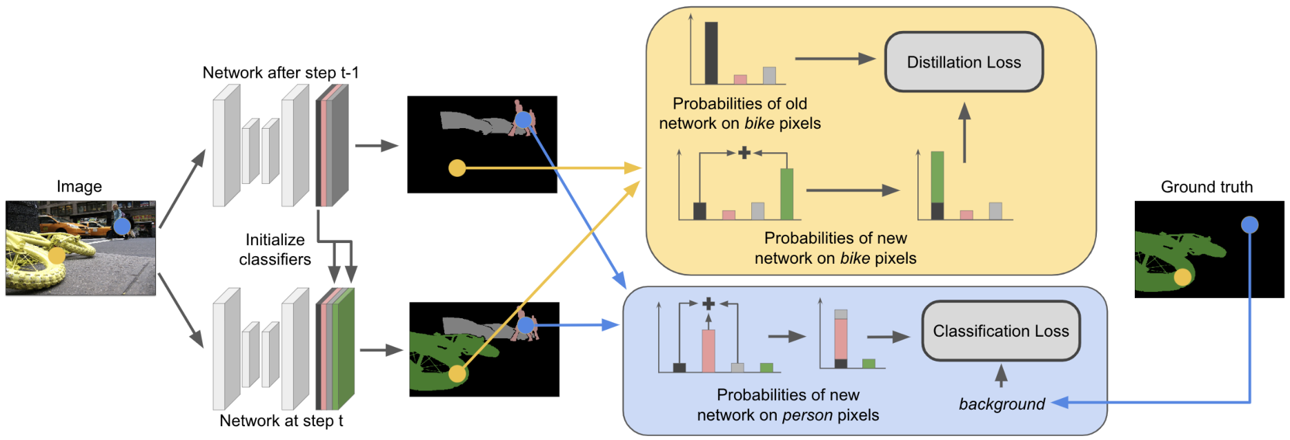
Our intuition is that by using Eq.(5) we can update the model to predict the new classes and, at the same time, account for the uncertainty over the actual content of the background class. In fact, in Eq. (5) the background class ground truth is not directly compared with its probabilities ${q}_{x}^{t}(i,\mathtt{b})$ obtained from the current model $f_{\theta^{t}}$, but with the probability of having either an old class or the background. A schematic representation of this procedure is depicted in Fig. 2 (blue block).

It is worth noting that the alternative of ignoring the unlabeled pixels within the cross-entropy loss is a worse solution than considering them as background. In fact, this would not allow the model to correctly update its classifier to update its representation of the background and to learn the boundary of novel objects. Moreover, it would not allow to exploit the information that new images might contain about old classes.

The rationale behind $\ell_{kd}$ is that $f_{\theta^{t}}$ should produce activations close to the ones produced by $f_{\theta^{t-1}}$. This regularizes the training procedure such that the parameters $\theta^{t}$ remain anchored to the solution found for classifying pixels of previous classes, i.e. $\theta^{t-1}$.

The loss defined in Eq. (7) has been used either in its base form or variants in different contexts, from incremental task [15] and class learning [13, 16] in object classification to complex scenarios such as detection [43] and segmentation [27]. Despite its success, it has a fundamental drawback in semantic segmentation: it completely ignores that the representation of the background class evolves over time. While with Eq. (5) we tackled the first problem linked to the semantic shift of the background (i.e. $\mathtt{b}\in\mathcal{T}^{t}$ contains pixels of $\mathcal{Y}^{t-1}$), we use the distillation loss to tackle the second: annotations for background in $\mathcal{T}^{s}$ with $s<t$ might include pixels of classes in $\mathcal{C}^{t}$. From the latter considerations, the background probabilities assigned to a pixel by the old predictor $f_{\theta^{t-1}}$ and by the current model $f_{\theta^{t}}$ do not share the same semantic content. More importantly, $f_{\theta^{t-1}}$ might predict as background pixels of classes in $\mathcal{C}^{t}$ that we are currently trying to learn. Notice that this aspect is peculiar to the segmentation task and it is not considered in previous incremental learning models.

To address the semantic shift of the background class between the old and the current model, we explicitly revise the distillation loss in Eq. (7). In particular, we extend the reasoning behind Sec.III-B to the distillation soft-targets and we design a novel distillation loss by rewriting the probability distribution $\hat{p}_{x}^{t}(i,c)$ in Eq. (8) as:

We note that Eq. (9) is identical to Eq. (2) by setting $\mathcal{U}=\mathcal{Y}^{t}$ and by substituting the background class $b$ to $\mathtt{u}$.

Similarly to Eq. (7), we still compare the probability of a pixel belonging to seen classes assigned by the old model, with its counterpart computed with the current parameters $\theta^{t}$. However, differently from classical distillation, in Eq. (9) the probabilities obtained with the current model are kept unaltered, i.e. normalized across the whole label space $\mathcal{Y}^{t}$ and not with respect to the subset $\mathcal{Y}^{t-1}$ (Eq. (8)). More importantly, the background class probability as given by $f_{\theta^{t-1}}$ is not directly compared with its counterpart in $f_{\theta^{t}}$, but with the probability of having either a new class or the background, as predicted by $f_{\theta^{t}}$ (see Fig. 2, yellow block).

We highlight that, with respect to Eq. (8) and other simple choices (e.g. ignoring unlabeled pixels from Eq. (8)) this solution has two advantages. First, we can use the full output space of the old model to distill knowledge in the current one, without ignoring any pixel or class. Second, we can propagate the uncertainty we have on the semantic content of the background in $f_{\theta^{t-1}}$ without penalizing the probabilities of new classes we are learning in the current step $t$.

To address this issue, we propose to initialize the classifier’s parameters for the novel classes in such a way that given an image $x$ and a pixel $i$, the probability of the background $q_{x}^{t-1}(i,\mathtt{b})$ is uniformly spread among the classes in $\mathcal{C}^{t}$, i.e. $q_{x}^{t}(i,c)=q_{x}^{t-1}(i,\mathtt{b})/|\mathcal{C}^{t}|\;\forall c\in\mathcal{C}^{t}$, where $|\mathcal{C}^{t}|$ is the number of new classes (notice that $\mathtt{b}\in\mathcal{C}^{t}$). To this extent, let us consider a standard fully connected classifier and let us denote as $\{\omega^{t}_{c},\beta^{t}_{c}\}\in\theta^{t}$ the classifier parameters for a class $c$ at learning step $t$, with $\omega$ and $\beta$ denoting its weights and bias respectively. We can initialize $\{\omega^{t}_{c},\beta^{t}_{c}\}$ as follows:

where $\{\omega_{\mathtt{b}}^{t-1},\beta_{\mathtt{b}}^{t-1}\}$ are the weights and bias of the background classifier at the previous learning step. The fact that the initialization defined in Eq.(10) and (11) leads to $q_{x}^{t}(i,c)=q_{x}^{t-1}(i,\mathtt{b})/|\mathcal{C}^{t}|\;\forall c\in\mathcal{C}^{t}$ is easy to obtain from $q_{x}^{t}(i,c)\propto\exp(\omega_{\mathtt{b}}^{t}\cdot x+\beta^{t}_{\mathtt{b}})$.

As we will show in the experimental analysis, this simple initialization procedure brings benefits in terms of both improving the learning stability of the model and the final results, since it eases the role of the supervision imposed by Eq.(5) while learning new classes and follows the same principles used to derive our distillation loss (Eq.(9)).

In weakly supervised segmentation using points or scribbles the goal is to obtain a model capable of predicting, for each pixel of the image, its correct semantic class, as in standard semantic segmentation. However, differently from the standard segmentation task, we train our model using a training set in which we do not have full pixel-level annotation, but just points or scribbles. In particular, for each instance of a class presented in a training image, only one or few contiguous annotated pixels are provided. Formally, considering an image $x$ and its label $y$ belonging to the training set $\mathcal{T}$, the annotation is provided only for pixels $\mathcal{I}^{x}_{S}=\{i:\;\forall\;i\in\mathcal{I}\;\text{s.t.}\;y_{i}\in\mathcal{Y}\}$, where $|\mathcal{I}^{x}_{S}|<<|\mathcal{I}|$. All the other image pixels are unlabeled.

We address three weakly semantic segmentation setting: point-based [12] and scribble-based [19] object segmentation, and point-based scene parsing [20]. The goal of object segmentation is to predict object classes in a target image, where the objects are countable things, such as cars, bikes, and dogs. All the pixels that do not fall in these categories are labeled as background, which is considered a class in the output space $\mathcal{Y}$ of our model, similarly to Sec. 2. Formally, given a training set $\mathcal{T}\subset\mathcal{X}\times(\mathcal{Y}\cup\mathtt{u})^{N}$, the goal is to learn a model able to predict, for each pixel $i$, a label $y_{i}\in(\mathcal{Y})$. Following the protocols defined in [12] and [19], the point annotations are given only for the objects, while no points are provided for the background class. Differently, the scribble annotations also contain a scribble for the background class.

Scene parsing, instead, is a more complex task where the goal is to obtain a model able to predict both countable things and stuff classes (i.e. all the non-countable classes, such as sky, road, ground, etc.). In this setting, all the pixels in the image contain a semantic category and the background class is not included in the label space. Formally, the goal is to learn a model able to map each pixel $i$ to a label $y_{i}\in\mathcal{Y}$. The mapping is learned using a training set $\mathcal{T}\subset\mathcal{X}\times(\mathcal{Y}\cup\mathtt{u})^{N}$.

Being provided few labeled pixels, previous approaches [12, 20] proposed to apply a cross-entropy loss directly on the labeled points. In particular, they defined a partial cross-entropy (PCE) loss that considered only the pixels for which an annotation is given. Formally, given an image $x$ and the respective annotation $y$, the PCE loss has the form:

This loss is crucial for the network to discriminate the classes and to localize them in the image. However, while this solution is simple and easy to implement, it completely discards the information provided by the unlabeled pixels. In Section III-B we showed a simple principle to extract value from them and in this section we will revisit the principle to adapt it in this scenario.

We start from the assumption that, for each instance of a class in the image it has been provided at least one labeled pixel. This assumption implies that we know which are the classes present in the image and that all the pixels in the image belong to one of those classes. Denoting the set of classes appearing in the label $y$ of an image $x$ as $\mathcal{U}_{x}=\{c:\exists\,i\in I^{x}_{S}\;\text{s.t.}\;c=y_{i}\}$ , we can use the loss in Eq. (1), with $\mathcal{U}=\mathcal{U}_{x}$ to consider the uncertainty we have on all the unlabeled pixels of the image. In particular, denoting as $\mathcal{I}^{x}_{u}=\mathcal{I}\setminus\mathcal{I}^{x}_{S}$ the set of unlabeled pixels, we propose to extend Eq. (1) as follows:

where $p_{x}$ is the probability distribution defined in Eq.(2) with $\mathcal{U}=\mathcal{U}_{x}$, and $\gamma$ is a hyper-parameter to weight the importance of unlabeled pixels since in this scenario unlabeled pixels are many more than the labeled ones.

Using the $\ell_{UNL}$ loss provides two important benefits to our training procedure when compared with $\ell_{PCE}$: (i) information from labeled pixels is propagated to unlabeled ones, providing an additional source of supervision; (ii) if the network predicts an unlabeled pixel as belonging to a class $c$ which is not in the current image (i.e. $c\notin\mathcal{U}_{x}$), receives a feedback on the error from the loss function.

To summarize, given a training set $\mathcal{T}$, we train the network to minimize the following objective function:

We note that this loss function can be applied without any modification both with point and scribble supervision to the object segmentation and to the scene parsing tasks. The only difference relies on the classes contained in the image, since for object segmentation the background class $\mathtt{b}$ belongs to every image, i.e. $\mathtt{b}\in\mathcal{U}_{x}\;\;\forall x\in\mathcal{T}$, while in scene parsing the background class is not considered. As far as we know, our method is the first applicable on point and scribble supervision both on object segmentation and scene parsing, achieving state of the art results without relying on any other prior learned on additional data (e.g. objectness prior [12]).

In this work, we use three datasets: Pascal-VOC 2012, ADE20K and Cityscapes. PASCAL-VOC 2012 [2] is a widely used benchmark that includes 20 foreground object classes. We use the extra annotation provided in [64], resulting in a dataset containing 10582 images in the training set and 1449 images in the validation. ADE20K [3] is a large-scale dataset that contains 150 classes. Differently from Pascal-VOC 2012, this dataset contains both stuff (e.g. sky, building, wall) and object classes. The dataset comprises more than 25K scene-centric images. Adopting the standard protocol [5] we use 20K images for training and we reported the results on the 2K images of the validation set. Cityscapes [18] is a dataset containing street-level images captured in central Europe that includes 19 classes, which are both objects or stuffs. The dataset provides high-resolution images with size $2048\times 1024$, which are splitted in 2975 images for training, 500 for validation and 1525 for testing. However, since the test set ground truth are not available, we report results on the validation set as done by [65]. We exclude from the training protocol the coarse-annotations, and we use only the fine-grained annotations.

References

- [1] J. Long, E. Shelhamer, and T. Darrell, “Fully convolutional networks for semantic segmentation,” in CVPR, 2015.
- [2] M. Everingham, L. Van Gool, C. K. I. Williams, J. Winn, and A. Zisserman, “The PASCAL Visual Object Classes Challenge 2012 (VOC2012) Results,” http://www.pascal-network.org/challenges/VOC/voc2012/workshop/index.html.
- [3] B. Zhou, H. Zhao, X. Puig, S. Fidler, A. Barriuso, and A. Torralba, “Scene parsing through ade20k dataset,” in CVPR, 2017.
- [4] L.-C. Chen, Y. Zhu, G. Papandreou, F. Schroff, and H. Adam, “Encoder-decoder with atrous separable convolution for semantic image segmentation,” in ECCV, 2018.
- [5] H. Zhao, J. Shi, X. Qi, X. Wang, and J. Jia, “Pyramid scene parsing network,” in CVPR, 2017.
- [6] G. Lin, A. Milan, C. Shen, and I. Reid, “Refinenet: Multi-path refinement networks for high-resolution semantic segmentation,” in CVPR, 2017.
- [7] Z. Zhang, X. Zhang, C. Peng, X. Xue, and J. Sun, “Exfuse: Enhancing feature fusion for semantic segmentation,” in ECCV, 2018.
- [8] L.-C. Chen, G. Papandreou, F. Schroff, and H. Adam, “Rethinking atrous convolution for semantic image segmentation,” 2017.
- [9] L.-C. Chen, G. Papandreou, I. Kokkinos, K. Murphy, and A. L. Yuille, “Deeplab: Semantic image segmentation with deep convolutional nets, atrous convolution, and fully connected crfs,” IEEE T-PAMI, vol. 40, no. 4, pp. 834–848, 2017.
- [10] L.-C. Chen, Y. Yang, J. Wang, W. Xu, and A. L. Yuille, “Attention to scale: Scale-aware semantic image segmentation,” in CVPR, 2016.
- [11] A. Kolesnikov and C. H. Lampert, “Seed, expand and constrain: Three principles for weakly-supervised image segmentation,” in European conference on computer vision. Springer, 2016, pp. 695–711.
- [12] A. Bearman, O. Russakovsky, V. Ferrari, and L. Fei-Fei, “What’s the point: Semantic segmentation with point supervision,” in European conference on computer vision. Springer, 2016, pp. 549–565.
- [13] S.-A. Rebuffi, A. Kolesnikov, G. Sperl, and C. H. Lampert, “icarl: Incremental classifier and representation learning,” in CVPR, 2017.
- [14] M. McCloskey and N. J. Cohen, “Catastrophic interference in connectionist networks: The sequential learning problem,” in Psychology of learning and motivation. Elsevier, 1989, vol. 24, pp. 109–165.
- [15] Z. Li and D. Hoiem, “Learning without forgetting,” IEEE T-PAMI, vol. 40, no. 12, pp. 2935–2947, 2017.
- [16] F. M. Castro, M. J. Marín-Jiménez, N. Guil, C. Schmid, and K. Alahari, “End-to-end incremental learning,” in ECCV, 2018.
- [17] G. Hinton, O. Vinyals, and J. Dean, “Distilling the knowledge in a neural network,” 2015.
- [18] M. Cordts, M. Omran, S. Ramos, T. Rehfeld, M. Enzweiler, R. Benenson, U. Franke, S. Roth, and B. Schiele, “The cityscapes dataset for semantic urban scene understanding,” in Proceedings of the IEEE conference on computer vision and pattern recognition, 2016, pp. 3213–3223.
- [19] D. Lin, J. Dai, J. Jia, K. He, and J. Sun, “Scribblesup: Scribble-supervised convolutional networks for semantic segmentation,” in Proceedings of the IEEE Conference on Computer Vision and Pattern Recognition, 2016, pp. 3159–3167.
- [20] R. Qian, Y. Wei, H. Shi, J. Li, J. Liu, and T. Huang, “Weakly supervised scene parsing with point-based distance metric learning,” in Proceedings of the AAAI Conference on Artificial Intelligence, vol. 33, 2019, pp. 8843–8850.
- [21] F. Cermelli, M. Mancini, S. R. Bulo, E. Ricci, and B. Caputo, “Modeling the background for incremental learning in semantic segmentation,” in Proceedings of the IEEE/CVF Conference on Computer Vision and Pattern Recognition, 2020, pp. 9233–9242.
- [22] V. Badrinarayanan, A. Kendall, and R. Cipolla, “Segnet: A deep convolutional encoder-decoder architecture for image segmentation,” IEEE T-PAMI, vol. 39, no. 12, pp. 2481–2495, 2017.
- [23] G. Ghiasi and C. C. Fowlkes, “Laplacian pyramid reconstruction and refinement for semantic segmentation,” in ECCV, 2016.
- [24] F. Ozdemir, P. Fuernstahl, and O. Goksel, “Learn the new, keep the old: Extending pretrained models with new anatomy and images,” in International Conference on Medical Image Computing and Computer-Assisted Intervention, 2018, pp. 361–369.
- [25] F. Ozdemir and O. Goksel, “Extending pretrained segmentation networks with additional anatomical structures,” International journal of computer assisted radiology and surgery, pp. 1–9, 2019.
- [26] O. Tasar, Y. Tarabalka, and P. Alliez, “Incremental learning for semantic segmentation of large-scale remote sensing data,” IEEE Journal of Selected Topics in Applied Earth Observations and Remote Sensing, vol. 12, no. 9, pp. 3524–3537, 2019.
- [27] U. Michieli and P. Zanuttigh, “Incremental learning techniques for semantic segmentation,” in ICCV-WS, 2019, pp. 0–0.
- [28] M. De Lange, R. Aljundi, M. Masana, S. Parisot, X. Jia, A. Leonardis, G. Slabaugh, and T. Tuytelaars, “Continual learning: A comparative study on how to defy forgetting in classification tasks,” 2019.
- [29] H. Shin, J. K. Lee, J. Kim, and J. Kim, “Continual learning with deep generative replay,” in NeurIPS, 2017.
- [30] S. Hou, X. Pan, C. C. Loy, Z. Wang, and D. Lin, “Learning a unified classifier incrementally via rebalancing,” in CVPR, 2019.
- [31] C. Wu, L. Herranz, X. Liu, J. van de Weijer, B. Raducanu et al., “Memory replay gans: Learning to generate new categories without forgetting,” in NeurIPS, 2018.
- [32] O. Ostapenko, M. Puscas, T. Klein, P. Jahnichen, and M. Nabi, “Learning to remember: A synaptic plasticity driven framework for continual learning,” in CVPR, 2019.
- [33] J. Kirkpatrick, R. Pascanu, N. Rabinowitz, J. Veness, G. Desjardins, A. A. Rusu, K. Milan, J. Quan, T. Ramalho, A. Grabska-Barwinska et al., “Overcoming catastrophic forgetting in neural networks,” Proceedings of the national academy of sciences, vol. 114, no. 13, pp. 3521–3526, 2017.
- [34] A. Chaudhry, P. K. Dokania, T. Ajanthan, and P. H. Torr, “Riemannian walk for incremental learning: Understanding forgetting and intransigence,” in ECCV, 2018.
- [35] F. Zenke, B. Poole, and S. Ganguli, “Continual learning through synaptic intelligence,” in ICML, 2017.
- [36] P. Dhar, R. V. Singh, K.-C. Peng, Z. Wu, and R. Chellappa, “Learning without memorizing,” in CVPR, 2019.
- [37] A. Mallya and S. Lazebnik, “Packnet: Adding multiple tasks to a single network by iterative pruning,” in CVPR, 2018.
- [38] A. Mallya, D. Davis, and S. Lazebnik, “Piggyback: Adapting a single network to multiple tasks by learning to mask weights,” in ECCV, 2018.
- [39] A. A. Rusu, N. C. Rabinowitz, G. Desjardins, H. Soyer, J. Kirkpatrick, K. Kavukcuoglu, R. Pascanu, and R. Hadsell, “Progressive neural networks,” 2016.
- [40] Y. Wu, Y. Chen, L. Wang, Y. Ye, Z. Liu, Y. Guo, and Y. Fu, “Large scale incremental learning,” in CVPR, 2019.
- [41] R. Aljundi, F. Babiloni, M. Elhoseiny, M. Rohrbach, and T. Tuytelaars, “Memory aware synapses: Learning what (not) to forget,” in ECCV, 2018.
- [42] E. Fini, S. Lathuilière, E. Sangineto, M. Nabi, and E. Ricci, “Online continual learning under extreme memory constraints,” ECCV, 2020.
- [43] K. Shmelkov, C. Schmid, and K. Alahari, “Incremental learning of object detectors without catastrophic forgetting,” in ICCV, 2017.
- [44] J. Lee, E. Kim, S. Lee, J. Lee, and S. Yoon, “Ficklenet: Weakly and semi-supervised semantic image segmentation using stochastic inference,” in Proceedings of the IEEE conference on computer vision and pattern recognition, 2019, pp. 5267–5276.
- [45] Z. Huang, X. Wang, J. Wang, W. Liu, and J. Wang, “Weakly-supervised semantic segmentation network with deep seeded region growing,” in Proceedings of the IEEE Conference on Computer Vision and Pattern Recognition, 2018, pp. 7014–7023.
- [46] G. Sun, W. Wang, J. Dai, and L. Van Gool, “Mining cross-image semantics for weakly supervised semantic segmentation,” in European conference on computer vision. Springer, 2020.
- [47] J. Dai, K. He, and J. Sun, “Boxsup: Exploiting bounding boxes to supervise convolutional networks for semantic segmentation,” in Proceedings of the IEEE international conference on computer vision, 2015, pp. 1635–1643.
- [48] G. Papandreou, L.-C. Chen, K. P. Murphy, and A. L. Yuille, “Weakly-and semi-supervised learning of a deep convolutional network for semantic image segmentation,” in Proceedings of the IEEE international conference on computer vision, 2015, pp. 1742–1750.
- [49] A. Khoreva, R. Benenson, J. Hosang, M. Hein, and B. Schiele, “Simple does it: Weakly supervised instance and semantic segmentation,” in Proceedings of the IEEE conference on computer vision and pattern recognition, 2017, pp. 876–885.
- [50] M. Tang, A. Djelouah, F. Perazzi, Y. Boykov, and C. Schroers, “Normalized cut loss for weakly-supervised cnn segmentation,” in Proceedings of the IEEE Conference on Computer Vision and Pattern Recognition, 2018, pp. 1818–1827.
- [51] S. J. Oh, R. Benenson, A. Khoreva, Z. Akata, M. Fritz, and B. Schiele, “Exploiting saliency for object segmentation from image level labels,” in 2017 IEEE conference on computer vision and pattern recognition (CVPR). IEEE, 2017, pp. 5038–5047.
- [52] J. Ahn and S. Kwak, “Learning pixel-level semantic affinity with image-level supervision for weakly supervised semantic segmentation,” in Proceedings of the IEEE Conference on Computer Vision and Pattern Recognition, 2018, pp. 4981–4990.
- [53] J. Ahn, S. Cho, and S. Kwak, “Weakly supervised learning of instance segmentation with inter-pixel relations,” in Proceedings of the IEEE/CVF Conference on Computer Vision and Pattern Recognition, 2019, pp. 2209–2218.
- [54] N. Araslanov and S. Roth, “Single-stage semantic segmentation from image labels,” in Proceedings of the IEEE/CVF Conference on Computer Vision and Pattern Recognition, 2020, pp. 4253–4262.
- [55] Y.-T. Chang, Q. Wang, W.-C. Hung, R. Piramuthu, Y.-H. Tsai, and M.-H. Yang, “Weakly-supervised semantic segmentation via sub-category exploration,” in Proceedings of the IEEE/CVF Conference on Computer Vision and Pattern Recognition, 2020, pp. 8991–9000.
- [56] B. Zhou, A. Khosla, A. Lapedriza, A. Oliva, and A. Torralba, “Learning deep features for discriminative localization,” in Proceedings of the IEEE conference on computer vision and pattern recognition, 2016, pp. 2921–2929.
- [57] R. R. Selvaraju, M. Cogswell, A. Das, R. Vedantam, D. Parikh, and D. Batra, “Grad-cam: Visual explanations from deep networks via gradient-based localization,” in Proceedings of the IEEE international conference on computer vision, 2017, pp. 618–626.
- [58] R. Adams and L. Bischof, “Seeded region growing,” IEEE Transactions on pattern analysis and machine intelligence, vol. 16, no. 6, pp. 641–647, 1994.
- [59] N. Srivastava, G. Hinton, A. Krizhevsky, I. Sutskever, and R. Salakhutdinov, “Dropout: a simple way to prevent neural networks from overfitting,” The journal of machine learning research, vol. 15, no. 1, pp. 1929–1958, 2014.
- [60] P. Arbeláez, J. Pont-Tuset, J. T. Barron, F. Marques, and J. Malik, “Multiscale combinatorial grouping,” in Proceedings of the IEEE conference on computer vision and pattern recognition, 2014, pp. 328–335.
- [61] C. Rother, V. Kolmogorov, and A. Blake, “” grabcut” interactive foreground extraction using iterated graph cuts,” ACM transactions on graphics (TOG), vol. 23, no. 3, pp. 309–314, 2004.
- [62] M. Tang, F. Perazzi, A. Djelouah, I. Ben Ayed, C. Schroers, and Y. Boykov, “On regularized losses for weakly-supervised cnn segmentation,” in Proceedings of the European Conference on Computer Vision (ECCV), 2018, pp. 507–522.
- [63] B. Wang, G. Qi, S. Tang, T. Zhang, Y. Wei, L. Li, and Y. Zhang, “Boundary perception guidance: a scribble-supervised semantic segmentation approach,” in IJCAI International Joint Conference on Artificial Intelligence, 2019.
- [64] B. Hariharan, P. Arbelaez, L. Bourdev, S. Maji, and J. Malik, “Semantic contours from inverse detectors,” in International Conference on Computer Vision (ICCV), 2011.
- [65] S. Rota Bulò, L. Porzi, and P. Kontschieder, “In-place activated batchnorm for memory-optimized training of dnns,” in CVPR, 2018.
- [66] K. He, X. Zhang, S. Ren, and J. Sun, “Deep residual learning for image recognition,” in CVPR, 2016.
- [67] S. Xie, R. Girshick, P. Dollár, Z. Tu, and K. He, “Aggregated residual transformations for deep neural networks,” in Proceedings of the IEEE conference on computer vision and pattern recognition, 2017, pp. 1492–1500.
- [68] P. Krähenbühl and V. Koltun, “Efficient inference in fully connected crfs with gaussian edge potentials,” Advances in neural information processing systems, vol. 24, pp. 109–117, 2011.
- [69] Y. Xian, S. Choudhury, Y. He, B. Schiele, and Z. Akata, “Semantic projection network for zero-and few-label semantic segmentation,” in Proceedings of the IEEE Conference on Computer Vision and Pattern Recognition, 2019, pp. 8256–8265.
![[Uncaptioned image]](2201.13338v1/bios/fabio.jpg) |
Fabio Cermelli is a Ph.D. student in Computer and Control Engineering at the Politecnico di Torino, funded by the Italian Insitute of Technology (IIT). He received his master thesis in Software Engineering (Computer Engineering) with honors at the Politecnico di Torino in 2018. He is member of the Visual Learning and Multimodal Applications Laboratory (VANDAL), supervised by Prof. Barbara Caputo. During his first year, he was a visiting Ph.D. student in the Technologies of Vision Laboratory at FBK. |