跳到论文正文
W Papers独立论文阅读器 arXiv:2201.13237 论文正文 计算阅读时间 · 0%
引用这篇论文根据当前论文元数据生成,正式投稿前建议核对。


License: arXiv.org perpetual non-exclusive license
arXiv:2201.13237v1 [math.NA] 11 Jan 2022

CDNNs: The coupled deep neural networks for coupling of the Stokes and Darcy-Forchheimer problems Thanks: .

Jing Yue Affiliation: School of Electrical and Control Engineering, School of Mathematics and Data Science, Shaanxi University of Science and Technology, Xi’an    Jian Li Thanks: Corresponding author(Jian Li) email: jianli@sust.edu.cn; jiaaanli@gmail.com. Affiliation: School of Electrical and Control Engineering, School of Mathematics and Data Science, Shaanxi University of Science and Technology, Xi’an    Wen Zhang Affiliation: School of Electrical and Control Engineering, School of Mathematics and Data Science, Shaanxi University of Science and Technology, Xi’an
Abstract

In this article, we present an efficient deep learning method called coupled deep neural networks (CDNNs) for coupled physical problems. Our method compiles the interface conditions of the coupled PDEs into the networks properly and can be served as an efficient alternative to the complex coupled problems. To impose energy conservation constraints, the CDNNs utilize simple fully connected layers and a custom loss function to perform the model training process as well as the physical property of the exact solution. The approach can be beneficial for the following reasons: Firstly, we sampled randomly and only input spatial coordinates without being restricted by the nature of samples. Secondly, our method is meshfree which makes it more efficient than the traditional methods. Finally, our method is parallel and can solve multiple variables independently at the same time. We give the theory to guarantee the convergence of the loss function and the convergence of the neural networks to the exact solution. Some numerical experiments are performed and discussed to demonstrate the performance of the proposed method.

Key words: Scientific computing, Machine learning, the Stokes equations, Darcy-Forchheimer problems, Beaver-Joseph-Saffman interface condition.

1 Introduction

The fluid flow between porous media and free-flow zones has extensive applications in hydrology, environmental science, and biofluid dynamics. A lot of researchers derive suitable mathematical and numerical models for fluid movement. The system can be viewed as a coupled problem with two physical systems interacting across an interface. The simplest mathematical formulation for the coupled problem is coupling of the Stokes and Darcy flow with proper interface conditions. The most suitable and popular interface conditions are called Beavers-Joseph-Saffman conditions [1]. However, Darcy’s law only provides a linear relationship between the gradient of pressure and velocity in the coupled model, which usually fails for complex physical problems. Forchheimer [2] conducted flow experiments in sand packs and recognized that for moderate Reynolds numbers (R​e>0.1Re>0.1 approximately), Darcy’s law is not adequate. He found that the pressure gradient and Darcy velocity should satisfy the Darcy-Forchheimer law. Since the great attention has received in the coupled model, a large number of traditional methods have been devoted to the coupled Stokes and Darcy flows problems [3, 4, 5, 6, 7, 8, 9, 10, 11, 12, 13]. However, the difficulty of the complicated high dimensional coupled problems causes the limitation of traditional methods.

Owing to the enormous potential in approximating high-dimensional nonlinear maps [17, 18, 19, 20, 21, 22, 23, 24], deep learning has attracted growing attention in many applications, such as image, speech, text recognition and scientific computing [14, 15, 16]. Many works have arisen based on the function approximation capabilities of the feed-forward fully-connected neural network to solve initial/boundary value problems [31, 32, 33, 34] in the past decades. The solution to the system of equations can be obtained by minimizing the loss function, which typically consists of the residual error of the governing Partial Differential Equations (PDEs) along with initial/boundary values. Resently, Raissi etc.[35, 36, 37] developed Physics Informed Neural Networks (PINNs) [38, 39, 40, 41, 42, 43]. Moreover, Sirignano and Spiliopoulos proposed the Deep learning Galerkin Method [45] for solving high dimensional PDEs. Additionally, some recent works have successfully solved the second-order linear elliptic equations and the high dimensional Stokes problems [25, 26, 27, 28]. Although several excellent works have been performed in applying deep learning to solve PDEs, the topic for solving complicated coupled interface problems remains to be investigated.

Considering the performance of deep learning for solving PDEs, our contribution is to design the CDNNs as an efficient alternative model for complicated coupled physical problems. We can encode any underlying physical laws naturally as prior information to obey the law of physics. To satisfy the differential operators, boundary conditions and divergence conditions, we train the neural networks on batches of randomly sampled points. The method only inputs random sampling spatial coordinates without considering the nature of samples. Notably, we take the interface conditions as the constraint for the CDNNs. The approach is parallel and solves multiple variables independently at the same time. Specially, the optimal solution can be obtained by using the appropriate optimization method instead of a linear combination of basic functions. Further more, we validate the convergence of the loss function under certain conditions and the convergence of the CDNNs to the exact solution. Several numerical experiments are conducted to investigate the performance of the CDNNs.

The article is organized as follows: Section 2 introduces the coupled model and the relation methodology. Section 3 discusses the convergence of the loss function J⁡(𝐔¯)J(\overline{\mathbf{U}}) and the convergence of the CDNNs to the exact solution. Section 4 reveals some numerical experiments to illustrate the efficiency of the CDNNs. The article ends with conclusion in section 5.

2 Methodology

Let ΩS\Omega_{S} and ΩD\Omega_{D} be two bounded and simply connected polygonal domains in ℝ2\mathbb{R}^{2} such that ∂ΩS∩∂ΩD=Γ≠∅\partial\Omega_{S}\cap\partial\Omega_{D}=\Gamma\neq\emptyset and ΩS∩ΩD=∅\Omega_{S}\cap\Omega_{D}=\emptyset. Then, let ΓS:=∂ΩS∖Γ,ΓD:=∂ΩD∖Γ\Gamma_{S}:=\partial\Omega_{S}\setminus\Gamma,\Gamma_{D}:=\partial\Omega_{D}\setminus\Gamma and 𝐧𝐒\bf{n}_{S} as the unit normal vector pointing from ΩS\Omega_{S} to ΩD\Omega_{D}, 𝐧D\mathbf{n}_{D} as the unit normal vector pointing from ΩD\Omega_{D} to ΩS\Omega_{S}, on the interface Γ\Gamma we have 𝐧D=−𝐧S\mathbf{n}_{D}=-\mathbf{n}_{S}. In addition, 𝐭\mathbf{t} represents the unit tangential vector along the interface Γ\Gamma. Figure 1 gives a schematic representation of the geometry.

When kinematic effects surpass viscous effects in a porous medium, the Darcy velocity 𝐮D\mathbf{u}_{D} and the pressure gradient ∇pD\nabla{p}_{D} does not satisfy a linear relation. Instead, a nonlinear approximation, known as the Darcy-Forchheimermodel, is considered. When it is imposed on the porous medium ΩD\Omega_{D} with homogeneous Dircihlet boundary condition on ΓD\Gamma_{D} the equations read:

∇⋅𝐮D\displaystyle\nabla\cdot\mathbf{u}_{D} =fD,i​n​ΩD,\displaystyle=f_{D},~~~in~\Omega_{D}, (1)
μρ​𝐊−1​𝐮D+βρ​∣𝐮D∣​𝐮D+∇pD\displaystyle\frac{\mu}{\rho}\mathbf{K}^{-1}\mathbf{u}_{D}+\frac{\beta}{\rho}\mid\mathbf{u}_{D}\mid\mathbf{u}_{D}+\nabla p_{D} =𝐠D,i​n​ΩD,\displaystyle=\mathbf{g}_{D},~~~in~\Omega_{D}, (2)
pD\displaystyle p_{D} =0,o​n​∂ΩD∖Γ,\displaystyle=0,~~~on~\partial\Omega_{D}\setminus\Gamma, (3)

where 𝐊\mathbf{K} is the permeability tensor, assumed to be uniformly positive definite and bounded, ρ\rho is the density of the fluid, μ\mu is its viscosity and β\beta is a dynamic viscosity, all assumed to be positive constants. In addition, 𝐠D\mathbf{g}_{D} and fDf_{D} are source terms. We remark that in this context we exploit homogeneous Dirichlet boundary condition, in fact, we can also consider homogeneous Neumann boundary condition, i.e., 𝐮D⋅𝐧D=0\mathbf{u}_{D}\cdot\mathbf{n}_{D}=0 on ΓD\Gamma_{D} and the arguments used in this paper are still true.

The fluid motion in ΩS\Omega_{S} is described by the Stokes equations:

−ν​Δ​𝐮S+∇pS\displaystyle-\nu\Delta\mathbf{u}_{S}+\nabla p_{S} =𝐟S,i​n​ΩS,\displaystyle=\mathbf{f}_{S},~~~in~\Omega_{S}, (4)
∇⋅𝐮S\displaystyle\nabla\cdot\mathbf{u}_{S} =0,o​n​ΩS,\displaystyle=0,~~~on~\Omega_{S}, (5)
𝐮S\displaystyle\mathbf{u}_{S} =0,o​n​∂ΩS∖Γ,\displaystyle=0,~~~on~\partial\Omega_{S}\setminus\Gamma, (6)

where ν>0\nu>0 denotes the viscosity of the fluid.

On the interface, we prescribe the following interface conditions

𝐮S⋅𝐧S\displaystyle\mathbf{u}_{S}\cdot\mathbf{n}_{S} =𝐮D⋅𝐧S,o​n​Γ,\displaystyle=\mathbf{u}_{D}\cdot\mathbf{n}_{S},~~~on~\Gamma, (7)
pS−ν​𝐧S​∂𝐮S∂𝐧S\displaystyle p_{S}-\nu\mathbf{n}_{S}\frac{\partial\mathbf{u}_{S}}{\partial\mathbf{n}_{S}} =pD,o​n​Γ,\displaystyle=p_{D},~~~on~\Gamma, (8)
−ν​𝐭​∂𝐮S∂𝐧S\displaystyle-\nu\mathbf{t}\frac{\partial\mathbf{u}_{S}}{\partial\mathbf{n}_{S}} =G​𝐮S⋅𝐭,o​n​Γ.\displaystyle=G\mathbf{u}_{S}\cdot\mathbf{t},~~~on~\Gamma. (9)

Condition (7) represents continuity of the fluid velocity’s normal components, (8) represents the balance of forces acting across the interface, and (9) is the Beaver-Joseph-Saffman condition [46]. The constant G>0G>0 is given and is usually obtained from experimental data.

Refer to caption
Figure 1: Coupled domain with interface Γ\Gamma.

For notational brevity, we set 𝐮¯=(𝐮S,𝐮D,pS,pD)\overline{\mathbf{u}}=(\mathbf{u}_{S},\mathbf{u}_{D},p_{S},p_{D}) and recall the classical Sobolev spaces

𝕏S0={vS∈[H1​(ΩS)]d:vS|ΓS=𝟎},\mathbb{X}_{S}^{0}=\{v_{S}\in[H^{1}(\Omega_{S})]^{d}:v_{S}|_{\Gamma_{S}}=\mathbf{0}\},
𝕐D={qD∈[W1,3/2​(ΩD)]2:qD|ΓD=0},\mathbb{Y}_{D}=\{q_{D}\in[W^{1,3/2}(\Omega_{D})]^{2}:q_{D}|_{\Gamma_{D}}=0\},
𝕏S={vS∈𝕏S0:d​i​v​vS=0},\mathbb{X}_{S}=\{v_{S}\in\mathbb{X}_{S}^{0}:div~v_{S}=0\},

where

Hk(Ω)={υ∈L2(Ω):Dwαυ∈L2(Ω),∀α:∣α∣≤k},H^{k}(\Omega)=\Big\{\upsilon\in L^{2}(\Omega):D_{w}^{\alpha}\upsilon\in L^{2}(\Omega),\forall\alpha:\mid\alpha\mid\leq k\Big\},

and their norm

∥υ∥k=(υ,υ)k={∑∣α∣=0k∫Ω(Dwαυ)2dx}12,∥υ∥Wk,p={∑|α|≤k∥υ∥Lpp}1/p.\parallel\upsilon\parallel_{k}=\sqrt{(\upsilon,\upsilon)_{k}}=\bigg\{\sum_{\mid\alpha\mid=0}^{k}\int_{\Omega}(D_{w}^{\alpha}\upsilon)^{2}dx\bigg\}^{\frac{1}{2}},~~\parallel\upsilon\parallel_{W_{k,p}}=\Big\{\sum_{|\alpha|\leq k}\|\upsilon\|^{p}_{L^{p}}\Big\}^{1/p}.

Particularly,

‖v‖k=‖v‖Wk,2\|v\|_{k}=\|v\|_{W^{k,2}}

where k>0k>0 is a positive integer and ∥υ∥0\parallel\upsilon\parallel_{0} denotes the norm on L2​(Ω)L^{2}(\Omega) or (L2​(Ω))2(L^{2}(\Omega))^{2}, Dwα​υD_{w}^{\alpha}\upsilon is the generalized derivative of υ\upsilon. Moreover, (⋅,⋅)D(\cdot,\cdot)_{D} represents the inner product in the domain DD and <⋅,⋅><\cdot,\cdot> represents the inner product on the interface Γ\Gamma.

Refer to caption
Figure 2: The structure of the CDNNs.

To solve coupling of the Stokes and Darcy-Forchheimer problems, we propose the CDNNs in Figure 2. Further more, we give observations of the state variable 𝐔¯​(x,θ)=(𝐔S​(x,θ1)CLOSE\overline{\mathbf{U}}(x;\theta)=\big(\mathbf{U}_{S}(x;\theta_{1}), 𝐔D​(x,θ2)\mathbf{U}_{D}(x;\theta_{2}), PS​(x,θ3)P_{S}(x;\theta_{3}), OPENPD​(x,θ4))P_{D}(x;\theta_{4})\big), which is the neural network solution to the coupled Stokes and Darcy-Forchheimer problem (1)-(9), (θ𝟏,θ𝟑)(\mathbf{\theta_{1}},\mathbf{\theta_{3}}) and (θ𝟐,θ𝟒)(\mathbf{\theta_{2}},\mathbf{\theta_{4}}) are the stacked parameters of θ\theta for Stokes and Darcy respectively. The following constrained optimization procedure aims to reconstruct the parameters θ\theta by minimizing the loss function

J⁡[𝐔¯]=JΩS∖Γ​[𝐔¯]+JΩD∖Γ​[𝐔¯]+JΓ​[𝐔¯].J[\overline{\mathbf{U}}]=J_{\Omega_{S}\setminus\Gamma}[\overline{\mathbf{U}}]+J_{\Omega_{D}\setminus\Gamma}[\overline{\mathbf{U}}]+J_{\Gamma}[\overline{\mathbf{U}}]. (10)

where

JΩS∖Γ​(𝐔¯)=‖𝐟S+ν​Δ​𝐔S​(x,θ1)−∇PS​(x,θ3)‖0,ΩS,ω12+‖∇⋅𝐔𝐒​(x,θ1)‖0,ΩS,ω12+‖𝐔𝐒​(x,θ1)‖0,∂ΩS∖Γ,ω22JΩD∖Γ​(𝐔¯)=‖fD−∇⋅𝐔D​(x,θ2)‖0,ΩD,ω12+‖μρ​𝐊−1​𝐔D​(x,θ2)+βρ​|𝐔D​(x,θ2)|​𝐔D​(x,θ2)+∇PD​(x,θ4)−𝐠D‖0,ΩD,ω12+‖PD​(x,θ4)‖0,∂ΩD∖Γ,ω22JΓ​(𝐔¯)=‖𝐔S​(x,θ1)⋅𝐧S−𝐔D​(x,θ2)⋅𝐧S‖0,Γ,ω32+‖PS​(x,θ3)−ν​𝐧S​∂𝐔S​(x,θ1)∂𝐧S−PD​(x,θ4)‖0,Γ,ω32+‖−ν​𝐭​∂𝐔S​(x,θ1)∂𝐧S−G​𝐔S​(x,θ1)⋅𝐭‖0,Γ,ω32\begin{split}J_{\Omega_{S}\setminus\Gamma}(\overline{\mathbf{U}})=&\Big\|\mathbf{f}_{S}+\nu\Delta\mathbf{U}_{S}(x;\theta_{1})-\nabla P_{S}(x;\theta_{3})\Big\|_{0,\Omega_{S},\omega_{1}}^{2}\\ &+\Big\|\nabla\cdot{\mathbf{U_{S}}}(x;\theta_{1})\Big\|_{0,\Omega_{S},\omega_{1}}^{2}+\Big\|\mathbf{U_{S}}(x;\theta_{1})\Big\|_{0,\partial\Omega_{S}\setminus\Gamma,\omega_{2}}^{2}\\ J_{\Omega_{D}\setminus\Gamma}(\overline{\mathbf{U}})=&\Big\|f_{D}-\nabla\cdot\mathbf{U}_{D}(x;\theta_{2})\Big\|_{0,\Omega_{D},\omega_{1}}^{2}\\ &+\Big\|\frac{\mu}{\rho}\mathbf{K}^{-1}\mathbf{U}_{D}(x;\theta_{2})+\frac{\beta}{\rho}\big|\mathbf{U}_{D}(x;\theta_{2})\big|\mathbf{U}_{D}(x;\theta_{2})+\nabla P_{D}(x;\theta_{4})-\mathbf{g}_{D}\Big\|_{0,\Omega_{D},\omega_{1}}^{2}\\ &+\Big\|P_{D}(x;\theta_{4})\Big\|_{0,\partial\Omega_{D}\setminus\Gamma,\omega_{2}}^{2}\\ J_{\Gamma}(\overline{\mathbf{U}})=&\Big\|\mathbf{U}_{S}(x;\theta_{1})\cdot\mathbf{n}_{S}-\mathbf{U}_{D}(x;\theta_{2})\cdot\mathbf{n}_{S}\Big\|_{0,\Gamma,\omega_{3}}^{2}\\ &+\Big\|P_{S}(x;\theta_{3})-\nu\mathbf{n}_{S}\frac{\partial\mathbf{U}_{S}(x;\theta_{1})}{\partial\mathbf{n}_{S}}-P_{D}(x;\theta_{4})\Big\|_{0,\Gamma,\omega_{3}}^{2}\\ &+\Big\|-\nu\mathbf{t}\frac{\partial\mathbf{U}_{S}(x;\theta_{1})}{\partial\mathbf{n}_{S}}-G\mathbf{U}_{S}(x;\theta_{1})\cdot\mathbf{t}\Big\|_{0,\Gamma,\omega_{3}}^{2}\\ \end{split} (11)

The nodal values of the parameters in the input layer admitted by the deep learning model. Furthermore, it should be noted that J⁡(𝐔¯)J(\overline{\mathbf{U}}) can measure how well the approximate solution satisfies differential operators, divergence conditions, boundary conditions and interface conditions. Notice that

‖f⁡(y)‖0,𝒴,ω=∫𝒴|f⁡(y)|2​ω​(y)​𝑑y,\big\|f(y)\big\|_{0,\mathcal{Y},\omega}=\int_{\mathcal{Y}}\big|f(y)\big|^{2}\omega(y)dy,

where ω⁡(y)\omega(y) is the probability density of yy in 𝒴\mathcal{Y}. Especially, if J⁡(𝐔¯)=0J(\overline{\mathbf{U}})=0 then 𝐔¯\overline{\mathbf{U}} is the solution to the coupled Stokes and Darcy-Forchheimer problems (1)-(9). Due to the infeasibility to estimate θ\theta by directly minimizing J⁡(𝐔¯)J(\overline{\mathbf{U}}) when integrated over a higher dimensional region, so we apply a sequence of randomly sampled points from domain instead forming mesh grid. The main steps of the CDNNs for the coupled Stokes and Darcy-Forchheimer equations are presented as Algorithm 1.

Input: ρω1(n)={xSn,xDn},ρω2(n)={rSn,rDn},ρω3(n)={rΓn)}\rho_{\omega_{1}}^{(n)}=\big\{x_{S}^{n},x_{D}^{n}\big\},\rho_{\omega_{2}}^{(n)}=\big\{r_{S}^{n},r_{D}^{n}\big\},\rho_{\omega_{3}}^{(n)}=\big\{r_{\Gamma}^{n})\big\}, max iterations MM, learning rate α\alpha
Output: θn+1\theta_{n+1}
1. Randomly generated sample points ρ(n)={ρω1(n),ρω2(n),ρω3(n)}\rho^{(n)}=\big\{\rho_{\omega_{1}}^{(n)},\rho_{\omega_{2}}^{(n)},\rho_{\omega_{3}}^{(n)}\big\} from (ΩS,ΩD)(\Omega_{S},\Omega_{D}), (∂ΩS\Γ,∂ΩD\Γ)(\partial\Omega_{S}\backslash\Gamma,\partial\Omega_{D}\backslash\Gamma) and Γ\Gamma by the respective probability densities ω1\omega_{1}, ω2\omega_{2} and ω3\omega_{3};
2. Initialize the parameters θ\theta;
3. while iterations ≤M\leq M do
read current;
G⁡(ρ(n),θn)\displaystyle G(\rho^{(n)},\theta^{n}) =GS​(ρ(n),θn)+GD​(ρ(n),θn)+GΓ​(ρ(n),θn),\displaystyle=G_{S}(\rho^{(n)},\theta^{n})+G_{D}(\rho^{(n)},\theta^{n})+G_{\Gamma}(\rho^{(n)},\theta^{n}),

where
GS​(ρ(n),θn)\displaystyle G_{S}(\rho^{(n)},\theta^{n}) =(𝐟S+ν​Δ​𝐔S​(xSn,θ1)−∇PS​(xSn,θ3))2\displaystyle=\Big(\mathbf{f}_{S}+\nu\Delta\mathbf{U}_{S}(x_{S}^{n};\theta_{1})-\nabla P_{S}(x_{S}^{n};\theta_{3})\Big)^{2}
+(∇⋅𝐔𝐒​(xSn,θ1))2+(𝐔𝐒​(rSn,θ1))2,\displaystyle+\Big(\nabla\cdot{\mathbf{U_{S}}}(x_{S}^{n};\theta_{1})\Big)^{2}+\Big(\mathbf{U_{S}}(r_{S}^{n};\theta_{1})\Big)^{2},
GD​(ρ(n),θn)\displaystyle G_{D}(\rho^{(n)},\theta^{n}) =(μρ​K−1​𝐔D​(xDn,θ2)+βρ​|𝐔D​(xDn,θ2)|​𝐔D​(xDn,θ2)+∇PD​(xDn,θ4)−𝐠D)2\displaystyle=\Big(\frac{\mu}{\rho}K^{-1}\mathbf{U}_{D}(x_{D}^{n};\theta_{2})+\frac{\beta}{\rho}\big|\mathbf{U}_{D}(x_{D}^{n};\theta_{2})\big|\mathbf{U}_{D}(x_{D}^{n};\theta_{2})+\nabla P_{D}(x_{D}^{n};\theta_{4})-\mathbf{g}_{D}\Big)^{2}
+(fD−∇⋅𝐔D​(xDn,θ2))2+(PD​(rDn,θ4))2,\displaystyle+\Big(f_{D}-\nabla\cdot\mathbf{U}_{D}(x_{D}^{n};\theta_{2})\Big)^{2}+\Big(P_{D}(r_{D}^{n};\theta_{4})\Big)^{2},

and
GΓ​(ρ(n),θn)\displaystyle G_{\Gamma}(\rho^{(n)},\theta^{n}) =(𝐔S​(x,θ1)⋅𝐧S−𝐔D​(x,θ2)⋅𝐧S)2\displaystyle=\Big(\mathbf{U}_{S}(x;\theta_{1})\cdot\mathbf{n}_{S}-\mathbf{U}_{D}(x;\theta_{2})\cdot\mathbf{n}_{S}\Big)^{2}
+(PS​(x,θ3)−ν​𝐧S​∂𝐔S​(x,θ1)𝐧S−PD​(x,θ4))2\displaystyle+\Big(P_{S}(x;\theta_{3})-\nu\mathbf{n}_{S}\frac{\partial\mathbf{U}_{S}(x;\theta_{1})}{\mathbf{n}_{S}}-P_{D}(x;\theta_{4})\Big)^{2}
+(−ν​𝐭​∂𝐔S​(x,θ1)∂𝐧S−G​𝐔S​(x,θ1)⋅𝐭)2,\displaystyle+\Big(-\nu\mathbf{t}\frac{\partial\mathbf{U}_{S}(x;\theta_{1})}{\partial\mathbf{n}_{S}}-G\mathbf{U}_{S}(x;\theta_{1})\cdot\mathbf{t}\Big)^{2},

and
θn+1=θn−α​∇θG​(ρ(n),θn).\theta^{n+1}=\theta_{n}-\alpha\nabla_{\theta}G(\rho^{(n)},\theta^{n}).

if limn→∞​‖∇θG​(ρ(n),θn)‖=0\underset{n\rightarrow\infty}{\lim}\|\nabla_{\theta}G(\rho^{(n)},\theta_{n})\|=0 then
    return the parameters θn+1\theta_{n+1};
       else
    go back to the beginning of current section.
Algorithm 1 The CDNNs for the coupled problems

Another noticeable point is that the term ∇θG​(θn,z(n))\nabla_{\theta}G(\theta^{n},z^{(n)}) is unbiased estimate of ∇θJ​(𝐔¯​(⋅,θn))\nabla_{\theta}J\big(\overline{\mathbf{U}}(\cdot;\theta^{n})\big) because the population parameters can be estimated by sample mathematical expectations.

3 Convergence

According to the definition of loss function J⁡(𝐔¯)J(\overline{\mathbf{U}}), it can measure how well 𝐔¯\overline{\mathbf{U}} satisfies the equations (1)-(9). Neural networks are a set of algorithms for classification and regression tasks inspired by the biological neural networks in brains. There have various types of neural networks with different neuron connection forms and architectures. According to the [20], if there is only one hidden layer and output, the set of functions implemented by following networks with m1,m2,m3m_{1},m_{2},m_{3} and m4m_{4} hidden units for coupling of the Stokes and Darcy-Forchheimer problems are

[ℭ𝐔Sm1​(φ)]d={Θ(x):ℝd↦ℝd|Θ(x)=∑i=1m1βiφ(∑j=1dσj,ixj+ci)},[ℭ𝐔Dm2​(ζ)]d={Λ(x):ℝd↦ℝd|Λ(x)=∑i=1m2β′iζ(∑j=1dσ′j,ixj+c′i)},ℭPSm3​(ψ)={Ψ(t,x):ℝd↦ℝ|Ψ(x)=∑i=1m3β′′iψ(∑j=1dσ′′j,ixj+c′′i)},ℭPDm4​(γ)={Υ(t,x):ℝd↦ℝ|Υ(x)=∑i=1m4β′′′iγ(∑j=1dσ′′′j,ixj+c′′′i)},\begin{split}[\mathfrak{C}_{\mathbf{U}_{S}}^{\mathrm{m_{1}}}(\varphi)]^{d}&=\Big\{\Theta(x):\mathbb{R^{\mathrm{d}}\mapsto\mathbb{R^{\mathrm{d}}}\Big|}\Theta(x)={\sum\limits_{i=1}^{m_{1}}}\beta_{i}\varphi\big({\sum\limits_{j=1}^{d}}\sigma_{j,i}x_{j}+c_{i}\big)\Big\},\\ [\mathfrak{C}_{\mathbf{U}_{D}}^{\mathrm{m_{2}}}(\zeta)]^{d}&=\Big\{\Lambda(x):\mathbb{R^{\mathrm{d}}\mapsto\mathbb{R^{\mathrm{d}}}\Big|}\Lambda(x)={\sum\limits_{i=1}^{m_{2}}}\beta^{\prime}_{i}\zeta\big({\sum\limits_{j=1}^{d}}\sigma^{\prime}_{j,i}x_{j}+c^{\prime}_{i}\big)\Big\},\\ \mathfrak{C}_{P_{S}}^{\mathrm{m_{3}}}(\psi)&=\Big\{\Psi(t,x):\mathbb{R^{\mathrm{d}}\mapsto\mathbb{R}\Big|}\Psi(x)={\sum\limits_{i=1}^{m_{3}}}\beta^{\prime\prime}_{i}\psi\big({\sum\limits_{j=1}^{d}}\sigma^{\prime\prime}_{j,i}x_{j}+c^{\prime\prime}_{i}\big)\Big\},\\ \mathfrak{C}_{P_{D}}^{\mathrm{m_{4}}}(\gamma)&=\Big\{\Upsilon(t,x):\mathbb{R^{\mathrm{d}}\mapsto\mathbb{R}\Big|}\Upsilon(x)={\sum\limits_{i=1}^{m_{4}}}\beta^{\prime\prime\prime}_{i}\gamma\big({\sum\limits_{j=1}^{d}}\sigma^{\prime\prime\prime}_{j,i}x_{j}+c^{\prime\prime\prime}_{i}\big)\Big\},\\ \end{split}

where Θ⁡(x)=(Θ1​(x),Θ2​(x),⋯,Θd​(x)),Λ⁡(x)=(Λ1​(x),Λ2​(x),⋯,Λd​(x))\Theta(x)=\big(\Theta_{1}(x),\Theta_{2}(x),\cdots,\Theta_{d}(x)\big),\Lambda(x)=\big(\Lambda_{1}(x),\Lambda_{2}(x),\cdots,\Lambda_{d}(x)\big), φ\varphi, ζ\zeta, ψ\psi and γ\gamma are the shared activation functions of the hidden units in 𝒞2​(Ω)\mathcal{C}^{2}(\Omega), bounded and non-constant. xjx_{j} is input, βi,βi′,βi′′,βi′′′,σj​i,σj​i′,σj​i′′\beta_{i},\beta^{\prime}_{i},\beta^{\prime\prime}_{i},\beta^{\prime\prime\prime}_{i},\sigma_{ji},\sigma^{\prime}_{ji},\sigma^{\prime\prime}_{ji}and σj​i′′′\sigma^{\prime\prime\prime}_{ji} are weights, ci,ci′,ci′′c_{i},c^{\prime}_{i},c^{\prime\prime}_{i} and ci′′′c^{\prime\prime\prime}_{i} are thresholds of the neural networks.

More generally, we use the similar notation

[ℭ𝐔S​(φ)]d×[ℭ𝐔D​(ζ)]d×ℭPS​(ψ)×ℭPD​(γ)[\mathfrak{C}_{\mathbf{U}_{S}}(\varphi)]^{d}\times[\mathfrak{C}_{\mathbf{U}_{D}}(\zeta)]^{d}\times\mathfrak{C}_{P_{S}}(\psi)\times\mathfrak{C}_{P_{D}}(\gamma)

for the multi layer neural networks with arbitrarily large number of hidden units m1,m2,m3m_{1},m_{2},m_{3} and m4m_{4}. In particular, the parameters and the activation function in each dimension of [ℭ𝐔Sm1​(φ)]d[\mathfrak{C}_{\mathbf{U}_{S}}^{m_{1}}(\varphi)]^{d} or [ℭ𝐔Dm2​(ζ)]d[\mathfrak{C}_{\mathbf{U}_{D}}^{\mathrm{m_{2}}}(\zeta)]^{d} are same as before, we set nn as the number of the neurons in numerical experiments. Then the parameters of the CDNNs can be formalized as follows

θ1k\displaystyle\theta_{1}^{k} =(β1,⋯,βn,σ11,⋯,σd​n,c1,⋯,cn),\displaystyle=(\beta_{1},\cdots,\beta_{n},\sigma_{11},\cdots,\sigma_{dn},c_{1},\cdots,c_{n}),
θ2k\displaystyle\theta_{2}^{k} =(β1′,⋯,βn,σ11′,⋯,σd​n′,c1′,⋯,cn′),\displaystyle=(\beta^{\prime}_{1},\cdots,\beta_{n},\sigma^{\prime}_{11},\cdots,\sigma^{\prime}_{dn},c^{\prime}_{1},\cdots,c^{\prime}_{n}),
θ3\displaystyle\theta_{3} =(β1′′,⋯,βn′,σ11′′,⋯,σd​n′′,c1′′,⋯,cn′′),\displaystyle=(\beta^{\prime\prime}_{1},\cdots,\beta^{\prime}_{n},\sigma^{\prime\prime}_{11},\cdots,\sigma^{\prime\prime}_{dn},c^{\prime\prime}_{1},\cdots,c^{\prime\prime}_{n}),
θ4\displaystyle\theta_{4} =(β1′′′,⋯,βn′′,σ11′′′,⋯,σd​n′′′,c1′′′,⋯,cn′′′),\displaystyle=(\beta^{\prime\prime\prime}_{1},\cdots,\beta^{\prime\prime}_{n},\sigma^{\prime\prime\prime}_{11},\cdots,\sigma^{\prime\prime\prime}_{dn},c^{\prime\prime\prime}_{1},\cdots,c^{\prime\prime\prime}_{n}),

where k=1,2,…,d,θ1∈ℝ(2+d)​n​d,θ2∈ℝ(2+d)​n​d,θ3∈ℝ(2+d)​nk=1,2,\ldots,d,\theta_{1}\in\mathbb{R}^{(2+d)nd},\theta_{2}\in\mathbb{R}^{(2+d)nd},\theta_{3}\in\mathbb{R}^{(2+d)n} and θ4∈ℝ(2+d)​n\theta_{4}\in\mathbb{R}^{(2+d)n}.

In the next two subsections, we prove that the neural network 𝐔¯n\overline{\mathbf{U}}^{n} with nn hidden units for 𝐔Sn,𝐔Dn,PSn\mathbf{U}_{S}^{n},\mathbf{U}_{D}^{n},P_{S}^{n} and PDnP_{D}^{n} satisfy the differential operators, boundary conditions, divergence conditions and interface conditions arbitrarily well for sufficiently large nn. More importantly, we confirm that there exists 𝐔¯n∈[ℭ𝐔S​(φ)]d×[ℭ𝐔D​(ζ)]d×ℭPS​(ψ)×ℭPD​(γ)\overline{\mathbf{U}}^{n}\in[\mathfrak{C}_{\mathbf{U}_{S}}(\varphi)]^{d}\times[\mathfrak{C}_{\mathbf{U}_{D}}(\zeta)]^{d}\times\mathfrak{C}_{P_{S}}(\psi)\times\mathfrak{C}_{P_{D}}(\gamma) such that J⁡(𝐔¯n)→0J(\overline{\mathbf{U}}^{n})\rightarrow 0 as n→∞n\rightarrow\infty. Another significant consideration, we give the convergence of 𝐔¯n→𝐮¯\overline{\mathbf{U}}^{n}\rightarrow\overline{\mathbf{u}} as n→∞n\rightarrow\infty where 𝐮¯\overline{\mathbf{u}} is the exact solution to the coupled equations (1)-(9).

3.1 Convergence of the loss function J⁡(𝐔¯)J(\overline{\mathbf{U}})

In this subsection, we prove the CDNNs 𝐔¯\overline{\mathbf{U}} can make the loss function J⁡(𝐔¯)J(\overline{\mathbf{U}}) arbitrarily small.

Assumption 3.1.

∇𝐯​(x),△​𝐯​(x)\nabla\mathbf{v}(x),\triangle\mathbf{v}(x) and ∇q​(x)\nabla q(x) are locally Lipschitz with Lipschitz coefficient that they have at most polynomial growth on 𝐯⁡(x)\mathbf{v}(x) and q⁡(x)q(x). Then, for some constants 0≤qi≤∞​(i=1,2,3,4)0\leq q_{i}\leq\infty(i=1,2,3,4) we have

|△​𝐕​(x,θ)−△​𝐯​(x)|≤(|∇𝐕​(x,θ)|q1/2+|∇𝐯​(x)|q2/2)​|∇𝐕​(x,θ)−∇v​(x)|,|\triangle\mathbf{V}(x;\theta)-\triangle\mathbf{v}(x)|\leq(|\nabla\mathbf{V}(x;\theta)|^{q_{1}/2}+|\nabla\mathbf{v}(x)|^{q_{2}/2})|\nabla\mathbf{V}(x;\theta)-\nabla v(x)|, (12)
|∇Q​(x,θ)−∇q​(x)|≤(|Q⁡(x,θ)|q3/2+|q⁡(x)|q4/2)​|Q⁡(x,θ)−q⁡(x)|,|\nabla Q(x;\theta)-\nabla q(x)|\leq(|Q(x;\theta)|^{q_{3}/2}+|q(x)|^{q_{4}/2})|Q(x;\theta)-q(x)|, (13)
|∇𝐕​(x,θ)−∇𝐯​(x)|≤(|𝐕⁡(x,θ)|q5/2+|𝐯⁡(x)|q6/2)​|𝐕⁡(x,θ)−𝐯⁡(x)|.|\nabla\mathbf{V}(x;\theta)-\nabla\mathbf{v}(x)|\leq(|\mathbf{V}(x;\theta)|^{q_{5}/2}+|\mathbf{v}(x)|^{q_{6}/2})|\mathbf{V}(x;\theta)-\mathbf{v}(x)|. (14)
Theorem 3.1.

Under the Assumption 3.1, there exists a neural network 𝐔¯∈[ℭ𝐔S​(φ)]d×[ℭ𝐔D​(ζ)]d×ℭPS​(ψ)×ℭPD​(γ)\overline{\mathbf{U}}\in[\mathfrak{C}_{\mathbf{U}_{S}}(\varphi)]^{d}\times[\mathfrak{C}_{\mathbf{U}_{D}}(\zeta)]^{d}\times\mathfrak{C}_{P_{S}}(\psi)\times\mathfrak{C}_{P_{D}}(\gamma), satisfying

J⁡(𝐔¯)≤C​ϵ2,∀ϵ>0,J(\overline{\mathbf{U}})\leq C\epsilon^{2},\ \forall\epsilon>0, (15)

where CC depends on the data {ΩS,ΩD,Γ,μ,ρ,β,K−1,ω1,ω2,ω3,fD,𝐠D,𝐟S}\{\Omega_{S},\Omega_{D},\Gamma,\mu,\rho,\beta,K^{-1},\omega_{1},\omega_{2},\omega_{3},f_{D},\mathbf{g}_{D},\mathbf{f}_{S}\}.

Proof.

From Theorem 3 of [20], we obtain that there exists 𝐔¯∈[ℭ𝐔S​(φ)]d×[ℭ𝐔D​(ζ)]d×ℭPS​(ψ)×ℭPD​(γ)\overline{\mathbf{U}}\in[\mathfrak{C}_{\mathbf{U}_{S}}(\varphi)]^{d}\times[\mathfrak{C}_{\mathbf{U}_{D}}(\zeta)]^{d}\times\mathfrak{C}_{P_{S}}(\psi)\times\mathfrak{C}_{P_{D}}(\gamma) which are uniformly 2-dense on compacts of 𝒞2​(Ω¯S)×𝒞2​(Ω¯D)×𝒞1​(Ω¯S)×𝒞1​(Ω¯D)\mathcal{C}^{2}(\bar{\Omega}_{S})\times\mathcal{C}^{2}(\bar{\Omega}_{D})\times\mathcal{C}^{1}(\bar{\Omega}_{S})\times\mathcal{C}^{1}(\bar{\Omega}_{D}). It means that for 𝐮¯​(x)∈𝒞2​(Ω¯S)×𝒞2​(Ω¯D)×𝒞1​(Ω¯S)×𝒞1​(Ω¯D),∀ϵ>0\overline{\mathbf{u}}(x)\in\mathcal{C}^{2}(\bar{\Omega}_{S})\times\mathcal{C}^{2}(\bar{\Omega}_{D})\times\mathcal{C}^{1}(\bar{\Omega}_{S})\times\mathcal{C}^{1}(\bar{\Omega}_{D}),\forall\epsilon>0, we confirm that

m​a​xa≤2​s​u​px∈ΩS​|∂xa𝐔S​(x,θ1)−∂xa𝐮S​(x)|<ϵ,\underset{a\leq 2}{max}\underset{x\in\Omega_{S}}{sup}|\partial_{x}^{a}\mathbf{U}_{S}(x;\theta_{1})-\partial_{x}^{a}\mathbf{u}_{S}(x)|<\epsilon, (16)
m​a​xa≤2​s​u​px∈ΩD​|∂xa𝐔D​(x,θ2)−∂xa𝐮D​(x)|<ϵ,\underset{a\leq 2}{max}\underset{x\in\Omega_{D}}{sup}|\partial_{x}^{a}\mathbf{U}_{D}(x;\theta_{2})-\partial_{x}^{a}\mathbf{u}_{D}(x)|<\epsilon, (17)
s​u​px∈ΩS​|PS​(x,θ3)−pS​(x)|<ϵ.\underset{x\in\Omega_{S}}{sup}|P_{S}(x;\theta_{3})-p_{S}(x)|<\epsilon. (18)
s​u​px∈ΩD​|PD​(x,θ4)−pD​(x)|<ϵ.\underset{x\in\Omega_{D}}{sup}|P_{D}(x;\theta_{4})-p_{D}(x)|<\epsilon. (19)

Firstly, we recall the form and discuss the convergence of JΩS∖Γ​(𝐔¯)J_{\Omega_{S}\setminus\Gamma}(\overline{\mathbf{U}}),

JΩS∖Γ​(𝐔¯)=‖𝐟S+ν​Δ​𝐔S​(x,θ1)−∇PS​(x,θ3)‖0,ΩS,ω12+‖∇⋅𝐔𝐒​(x,θ1)‖0,ΩS,ω12+‖𝐔𝐒​(x,θ1)‖0,∂ΩS∖Γ,ω22\begin{split}J_{\Omega_{S}\setminus\Gamma}(\overline{\mathbf{U}})&=\Big\|\mathbf{f}_{S}+\nu\Delta\mathbf{U}_{S}(x;\theta_{1})-\nabla P_{S}(x;\theta_{3})\Big\|_{0,\Omega_{S},\omega_{1}}^{2}\\ &+\Big\|\nabla\cdot{\mathbf{U_{S}}}(x;\theta_{1})\Big\|_{0,\Omega_{S},\omega_{1}}^{2}+\Big\|\mathbf{U_{S}}(x;\theta_{1})\Big\|_{0,\partial\Omega_{S}\setminus\Gamma,\omega_{2}}^{2}\\ \end{split} (20)

According to the Assumption 3.1, by using the Ho¨\ddot{o}lder inequality and Young inequality, setting conjugate numbers r1r_{1} and r2r_{2} such that 1r1+1r2=1\frac{1}{r_{1}}+\frac{1}{r_{2}}=1, it follows that

\displaystyle ∫ΩS|△​𝐔​(x,θ1)−△​𝐮​(x)|2​d​ω1​(x)\displaystyle\int_{\Omega_{S}}|\triangle\mathbf{U}(x;\theta_{1})-\triangle\mathbf{u}(x)|^{2}d\omega_{1}(x) (21)
≤\displaystyle\leq ∫ΩS(|∇𝐔​(x,θ1)|l1+|∇𝐮​(x)|l2)​(∇𝐔​(x,θ1)−∇𝐮​(x))2​d​ω1​(x)\displaystyle\int_{\Omega_{S}}\Big(|\nabla\mathbf{U}(x;\theta_{1})|^{l_{1}}+|\nabla\mathbf{u}(x)|^{l_{2}}\Big)\Big(\nabla\mathbf{U}(x;\theta_{1})-\nabla\mathbf{u}(x)\Big)^{2}d\omega_{1}(x)
≤\displaystyle\leq [∫ΩS(|∇𝐔​(x,θ1)|l1+|∇𝐮​(x)|l2)r1​d​ω1​(x)]1/r1\displaystyle\Big[\int_{\Omega_{S}}\Big(|\nabla\mathbf{U}(x;\theta_{1})|^{l_{1}}+|\nabla\mathbf{u}(x)|^{l_{2}}\Big)^{r_{1}}d\omega_{1}(x)\Big]^{1/r_{1}}
×[∫ΩS(∇𝐔​(x,θ1)−∇𝐮​(x))2​r2​d​ω1​(x)]1/r2\displaystyle\times\Big[\int_{\Omega_{S}}\Big(\nabla\mathbf{U}(x;\theta_{1})-\nabla\mathbf{u}(x)\Big)^{2r_{2}}d\omega_{1}(x)\Big]^{1/r_{2}}
≤\displaystyle\leq [∫ΩS(|∇𝐔​(x,θ1)−∇𝐮​(x)|l1+|∇𝐮​(x)|l1∨l2)r1​d​ω1​(x)]1/r1\displaystyle\Big[\int_{\Omega_{S}}\Big(|\nabla\mathbf{U}(x;\theta_{1})-\nabla\mathbf{u}(x)|^{l_{1}}+|\nabla\mathbf{u}(x)|^{l_{1}\vee l_{2}}\Big)^{r_{1}}d\omega_{1}(x)\Big]^{1/r_{1}}
×[∫ΩS(∇𝐔​(x,θ1)−∇𝐮​(x))2​r2​d​ω1​(x)]1/r2\displaystyle\times\Big[\int_{\Omega_{S}}\Big(\nabla\mathbf{U}(x;\theta_{1})-\nabla\mathbf{u}(x)\Big)^{2r_{2}}d\omega_{1}(x)\Big]^{1/r_{2}}
≤\displaystyle\leq OPENC⁡(ϵl1+s​u​pΩS​|∇𝐮​(x)|l1∨l2))​ϵ2,\displaystyle C\Big(\epsilon^{l_{1}}+\underset{{\Omega}_{S}}{sup}|\nabla\mathbf{u}(x)|^{l_{1}\vee l_{2}})\Big)\epsilon^{2},

here we set l1∨l2=m​a​x​{l1,l2}l_{1}\vee l_{2}=max\{l_{1},l_{2}\}. In the same way,

\displaystyle ∫ΩS|∇PS​(x,θ3)−∇pS​(x)|2​d​ω1​(x)\displaystyle\int_{\Omega_{S}}\Big|\nabla P_{S}(x;\theta_{3})-\nabla p_{S}(x)\Big|^{2}d\omega_{1}(x) (22)
≤\displaystyle\leq ∫ΩS(|PS​(x,θ3)|l3+|pS​(x)|l4)​(PS​(x,θ3)−pS​(x))2​d​ω1​(x)\displaystyle\int_{\Omega_{S}}\Big(|P_{S}(x;\theta_{3})|^{l_{3}}+|p_{S}(x)|^{l_{4}}\Big)\Big(P_{S}(x;\theta_{3})-p_{S}(x)\Big)^{2}d\omega_{1}(x)
≤\displaystyle\leq [∫ΩS(|PS​(x,θ3)|l3+|pS|l4)r3​d​ω1​(x)]1/r3×[∫ΩS(PS​(x,θ3)−pS​(x))2​r4​d​ω1​(x)]1/r4\displaystyle\Big[\int_{\Omega_{S}}\Big(|P_{S}(x;\theta_{3})|^{l_{3}}+|p_{S}|^{l_{4}}\Big)^{r_{3}}d\omega_{1}(x)\Big]^{1/r_{3}}\times\Big[\int_{\Omega_{S}}\Big(P_{S}(x;\theta_{3})-p_{S}(x)\Big)^{2r_{4}}d\omega_{1}(x)\Big]^{1/r_{4}}
≤\displaystyle\leq [∫ΩS(|PS​(x,θ3)−pS​(x)|l3+|pS​(x)|l3∨l4)r3​d​ω1​(x)]1/r3×[∫ΩS(PS​(x,θ3)−pS​(x))2​r4​d​ω1​(x)]1/r4\displaystyle\Big[\int_{\Omega_{S}}\Big(|P_{S}(x;\theta_{3})-p_{S}(x)|^{l_{3}}+|p_{S}(x)|^{l_{3}\vee l_{4}}\Big)^{r_{3}}d\omega_{1}(x)\Big]^{1/r_{3}}\times\Big[\int_{\Omega_{S}}\Big(P_{S}(x;\theta_{3})-p_{S}(x)\Big)^{2r_{4}}d\omega_{1}(x)\Big]^{1/r_{4}}
≤\displaystyle\leq OPENC⁡(ϵl3+s​u​pΩS​|pS​(x)|l3∨l4))​ϵ2,\displaystyle C\Big(\epsilon^{l_{3}}+\underset{{\Omega}_{S}}{sup}|p_{S}(x)|^{l_{3}\vee l_{4}})\Big)\epsilon^{2},

where 1r3+1r4=1\frac{1}{r_{3}}+\frac{1}{r_{4}}=1 and l3∨l4=m​a​x​{l3,l4}l_{3}\vee l_{4}=max\{l_{3},l_{4}\}.

For the boundary condition, we have

∫∂ΩS∖Γ|US​(x,θ1)−uS​(x)|2​d​ω2​(x)≤C​ϵ2.\displaystyle\int_{\partial\Omega_{S}\setminus\Gamma}|U_{S}(x;\theta_{1})-u_{S}(x)|^{2}d\omega_{2}(x)\leq C\epsilon^{2}. (23)

Owing to (21) - (23), we can conclude that

JΩS∖Γ​(𝐔¯)=\displaystyle J_{\Omega_{S}\setminus\Gamma}(\overline{\mathbf{U}})= ‖𝐟S+ν​Δ​𝐔S​(x,θ1)−∇PS​(x,θ3)‖0,ΩS,ω12\displaystyle\Big\|\mathbf{f}_{S}+\nu\Delta\mathbf{U}_{S}(x;\theta_{1})-\nabla P_{S}(x;\theta_{3})\Big\|_{0,\Omega_{S},\omega_{1}}^{2} (24)
+‖∇⋅𝐔𝐒​(x,θ1)‖0,ΩS,ω12+‖𝐔𝐒​(x,θ1)‖0,∂ΩS∖Γ,ω22\displaystyle+\Big\|\nabla\cdot{\mathbf{U_{S}}}(x;\theta_{1})\Big\|_{0,\Omega_{S},\omega_{1}}^{2}+\Big\|\mathbf{U_{S}}(x;\theta_{1})\Big\|_{0,\partial\Omega_{S}\setminus\Gamma,\omega_{2}}^{2}
≤\displaystyle\leq ν​‖Δ​𝐔S​(x,θ1)−Δ​𝐮S​(x)‖0,ΩS,ω12+‖∇PS​(x,θ3)−∇pS​(x)‖0,ΩS,ω12\displaystyle\nu\big\|\Delta\mathbf{U}_{S}(x;\theta_{1})-\Delta\mathbf{u}_{S}(x)\big\|_{0,\Omega_{S},\omega_{1}}^{2}+\big\|\nabla{P_{S}}(x;\theta_{3})-\nabla p_{S}(x)\big\|_{0,\Omega_{S},\omega_{1}}^{2}
+‖∇⋅𝐔S​(x,θ1)‖0,ΩS,ω12+‖𝐔⁡(x,θ1)‖0,∂ΩS∖Γ,ω22\displaystyle+\big\|\nabla\cdot{\mathbf{U}_{S}}(x;\theta_{1})\big\|_{0,\Omega_{S},\omega_{1}}^{2}+\big\|\mathbf{U}(x;\theta_{1})\big\|_{0,\partial\Omega_{S}\setminus\Gamma,\omega_{2}}^{2}
≤\displaystyle\leq ν​∫ΩS|△​𝐔S​(x,θ1)−△​𝐮S​(x)|2​d​ω1​(x)+∫ΩS|∇PS​(x,θ3)−∇pS​(x)|2​d​ω1​(x)\displaystyle\nu\int_{\Omega_{S}}|\triangle\mathbf{U}_{S}(x;\theta_{1})-\triangle\mathbf{u}_{S}(x)|^{2}d\omega_{1}(x)+\int_{\Omega_{S}}|\nabla P_{S}(x;\theta_{3})-\nabla p_{S}(x)|^{2}d\omega_{1}(x)
+∫ΩS|∇⋅𝐮S(x)|2dω1(x)+∫ΩS|∇⋅(𝐔S(x;θ1)−𝐮S(x))|2dω1(x)\displaystyle+\int_{\Omega_{S}}|\nabla\cdot\mathbf{u}_{S}(x)|^{2}d\omega_{1}(x)+\int_{\Omega_{S}}\Big|\nabla\cdot\Big(\mathbf{U}_{S}(x;\theta_{1})-\mathbf{u}_{S}(x)\Big)\Big|^{2}d\omega_{1}(x)
+∫∂ΩS∖Γ|𝐔S(x;θ1)−𝐮S(x)|2dω2(x)\displaystyle+\int_{\partial\Omega_{S}\setminus\Gamma}|\mathbf{U}_{S}(x;\theta_{1})-\mathbf{u}_{S}(x)|^{2}d\omega_{2}(x)
≤\displaystyle\leq C​ϵ2.\displaystyle C\epsilon^{2}.

Next, we remain to prove the convergence of JΩD∖Γ​(𝐔¯)J_{\Omega_{D}\setminus\Gamma}(\overline{\mathbf{U}}) and JΓ​(𝐔¯)J_{\Gamma}(\overline{\mathbf{U}}). We know that

JΩD∖Γ​(𝐔¯)=‖fD−∇⋅𝐔D​(x,θ2)‖0,ΩD,ω12+‖PD​(x,θ4)‖0,∂ΩD∖Γ,ω22+‖μρ​K−1​𝐔D​(x,θ2)+βρ​|𝐔D​(x,θ2)|​𝐔D​(x,θ2)+∇PD​(x,θ4)−𝐠D‖0,ΩD,ω12.\begin{split}J_{\Omega_{D}\setminus\Gamma}(\overline{\mathbf{U}})=&\Big\|f_{D}-\nabla\cdot\mathbf{U}_{D}(x;\theta_{2})\Big\|_{0,\Omega_{D},\omega_{1}}^{2}+\Big\|P_{D}(x;\theta_{4})\Big\|_{0,\partial\Omega_{D}\setminus\Gamma,\omega_{2}}^{2}\\ &+\Big\|\frac{\mu}{\rho}K^{-1}\mathbf{U}_{D}(x;\theta_{2})+\frac{\beta}{\rho}\big|\mathbf{U}_{D}(x;\theta_{2})\big|\mathbf{U}_{D}(x;\theta_{2})+\nabla P_{D}(x;\theta_{4})-\mathbf{g}_{D}\Big\|_{0,\Omega_{D},\omega_{1}}^{2}.\end{split} (25)

From (19), we have

∫ΩD|∇PD​(x,θ4)−∇pD​(x)|2​d​ω1​(x)\displaystyle\int_{\Omega_{D}}\Big|\nabla P_{D}(x;\theta_{4})-\nabla p_{D}(x)\Big|^{2}d\omega_{1}(x) (26)
≤\displaystyle\leq ∫ΩD(|PD​(x,θ4)|l5+|pD​(x)|l6)​(PD​(x,θ4)−pD​(x))2​d​ω1​(x),\displaystyle\int_{\Omega_{D}}\Big(|P_{D}(x;\theta_{4})|^{l_{5}}+|p_{D}(x)|^{l_{6}}\Big)\Big(P_{D}(x;\theta_{4})-p_{D}(x)\Big)^{2}d\omega_{1}(x),

which can be updated by using the Ho¨\ddot{o}lder inequality and Young inequality, thus we have

[∫ΩD(|PD​(x,θ4)|l5+|pD|l6)r5​d​ω1​(x)]1/r5\displaystyle\Big[\int_{\Omega_{D}}\Big(|P_{D}(x;\theta_{4})|^{l_{5}}+|p_{D}|^{l_{6}}\Big)^{r_{5}}d\omega_{1}(x)\Big]^{1/r_{5}} (27)
×[∫ΩD(PD(x;θ4)−pD(x))|2​r6dω1(x)]1/r6\displaystyle\times\Big[\int_{\Omega_{D}}(P_{D}(x;\theta_{4})-p_{D}(x))|^{2r_{6}}d\omega_{1}(x)\Big]^{1/r_{6}}
≤\displaystyle\leq [∫ΩD(|PD​(x,θ4)−pD​(x)|l5+|pD​(x)|l5∨l6)r5​d​ω1​(x)]1/r5\displaystyle\Big[\int_{\Omega_{D}}\Big(|P_{D}(x;\theta_{4})-p_{D}(x)|^{l_{5}}+|p_{D}(x)|^{l_{5}\vee l_{6}}\Big)^{r_{5}}d\omega_{1}(x)\Big]^{1/r_{5}}
×[∫ΩD(PD​(x,θ4)−pD​(x))2​r6​d​ω1​(x)]1/r6\displaystyle\times\Big[\int_{\Omega_{D}}\Big(P_{D}(x;\theta_{4})-p_{D}(x)\Big)^{2r_{6}}d\omega_{1}(x)\Big]^{1/r_{6}}
≤\displaystyle\leq OPENC⁡(ϵl5+s​u​pΩD​|pD​(x)|l5∨l6))​ϵ2,\displaystyle C\Big(\epsilon^{l_{5}}+\underset{{\Omega}_{D}}{sup}|p_{D}(x)|^{l_{5}\vee l_{6}})\Big)\epsilon^{2},

where 1r5+1r6=1\frac{1}{r_{5}}+\frac{1}{r_{6}}=1 and l5∨l6=m​a​x​{l5,l6}l_{5}\vee l_{6}=max\{l_{5},l_{6}\}.

Next we prove the boundedness of term |𝐔D​(x,θ2)|​𝐔D​(x,θ2)|\mathbf{U}_{D}(x;\theta_{2})\big|\mathbf{U}_{D}(x;\theta_{2}),

∫ΩD(|𝐔D​(x,θ2)|​𝐔D​(x,θ2)−|𝐮D​(x)|​𝐮D​(x))2​d​ω1​(x)=∫ΩD(𝐔D​(x,θ2)​(|𝐔D​(x,θ2)|−|𝐮D​(x)|)+|𝐮D​(x)|​(𝐔D​(x,θ2)−𝐮D​(x)))2​d​ω1​(x)=∫ΩD(𝐔D​(x,θ2)​(|𝐔D​(x,θ2)|−|𝐮D​(x)|))2​d​ω1​(x)+∫ΩD(|𝐮D​(x)|​(𝐔D​(x,θ2)−𝐮D​(x)))2​d​ω1​(x)+2∫ΩD(|𝐮D(x)|𝐔D(x;θ2)(|𝐔D(x;θ2)|−|𝐮D(x)|)(𝐔D(x;θ2)−𝐮D(x))dω1(x),\begin{split}&\int_{\Omega_{D}}\Big(|\mathbf{U}_{D}(x;\theta_{2})\big|\mathbf{U}_{D}(x;\theta_{2})-|\mathbf{u}_{D}(x)\big|\mathbf{u}_{D}(x)\Big)^{2}d\omega_{1}(x)\\ =&\int_{\Omega_{D}}\Big(\mathbf{U}_{D}(x;\theta_{2})\Big(|\mathbf{U}_{D}(x;\theta_{2})|-|\mathbf{u}_{D}(x)|\Big)+|\mathbf{u}_{D}(x)|\Big(\mathbf{U}_{D}(x;\theta_{2})-\mathbf{u}_{D}(x)\Big)\Big)^{2}d\omega_{1}(x)\\ =&\int_{\Omega_{D}}\Big(\mathbf{U}_{D}(x;\theta_{2})\Big(|\mathbf{U}_{D}(x;\theta_{2})|-|\mathbf{u}_{D}(x)|\Big)\Big)^{2}d\omega_{1}(x)+\int_{\Omega_{D}}\Big(|\mathbf{u}_{D}(x)|\Big(\mathbf{U}_{D}(x;\theta_{2})-\mathbf{u}_{D}(x)\Big)\Big)^{2}d\omega_{1}(x)\\ &+2\int_{\Omega_{D}}\Big(|\mathbf{u}_{D}(x)|\mathbf{U}_{D}(x;\theta_{2})\Big(|\mathbf{U}_{D}(x;\theta_{2})|-|\mathbf{u}_{D}(x)|\Big)\Big(\mathbf{U}_{D}(x;\theta_{2})-\mathbf{u}_{D}(x)\Big)d\omega_{1}(x),\end{split} (28)

where

∫ΩD(𝐔D​(x,θ2)​(|𝐔D​(x,θ2)|−|𝐮D​(x)|))2​d​ω1​(x)\displaystyle\int_{\Omega_{D}}\Big(\mathbf{U}_{D}(x;\theta_{2})\Big(|\mathbf{U}_{D}(x;\theta_{2})|-|\mathbf{u}_{D}(x)|\Big)\Big)^{2}d\omega_{1}(x) (29)
≤\displaystyle\leq [∫ΩD(𝐔D(x;θ2))2​r7dω1(x)]1/r7×[∫ΩD(|𝐔D(x;θ2)|+|𝐮D(x)|))2​r8dω1(x)]r8\displaystyle\Big[\int_{\Omega_{D}}\Big(\mathbf{U}_{D}(x;\theta_{2})\Big)^{2r_{7}}d\omega_{1}(x)\Big]^{1/{r_{7}}}\times\Big[\int_{\Omega_{D}}\Big(|\mathbf{U}_{D}(x;\theta_{2})|+|\mathbf{u}_{D}(x)|\Big)\Big)^{2r_{8}}d\omega_{1}(x)\Big]^{r_{8}}
≤\displaystyle\leq [∫ΩD((𝐔D​(x,θ2)−𝐮D​(x))+𝐮D​(x))2​r7​d​ω1​(x)]1/r7\displaystyle\Big[\int_{\Omega_{D}}\Big(\Big(\mathbf{U}_{D}(x;\theta_{2})-\mathbf{u}_{D}(x)\Big)+\mathbf{u}_{D}(x)\Big)^{2r_{7}}d\omega_{1}(x)\Big]^{1/{r_{7}}}
×[∫ΩD(|𝐔D​(x,θ2)−𝐮D​(x)|+|𝐮D​(x)|)2​r8​d​ω1​(x)]r8,\displaystyle\times\Big[\int_{\Omega_{D}}\Big(|\mathbf{U}_{D}(x;\theta_{2})-\mathbf{u}_{D}(x)|+|\mathbf{u}_{D}(x)|\Big)^{2r_{8}}d\omega_{1}(x)\Big]^{r_{8}},

by using the Ho¨\ddot{o}lder inequality and Young inequality, setting conjugate numbers r7r_{7} and r8r_{8} such that 1r7+1r8=1\frac{1}{r_{7}}+\frac{1}{r_{8}}=1.

Similarly, we can obtain

∫ΩD(|𝐮D​(x)|​(𝐔D​(x,θ2)−𝐮D​(x)))2​d​ω1​(x)\displaystyle\int_{\Omega_{D}}\Big(|\mathbf{u}_{D}(x)|\Big(\mathbf{U}_{D}(x;\theta_{2})-\mathbf{u}_{D}(x)\Big)\Big)^{2}d\omega_{1}(x) (30)
≤\displaystyle\leq [∫ΩD(|𝐮D(x)|)r9]1/r9×[∫ΩD(𝐔D(x;θ2)−𝐮D(x)))2​r10]1/r10dω1(x),\displaystyle[\int_{\Omega_{D}}\Big(|\mathbf{u}_{D}(x)|)^{r_{9}}]^{1/r_{9}}\times[\int_{\Omega_{D}}\Big(\mathbf{U}_{D}(x;\theta_{2})-\mathbf{u}_{D}(x)\Big)\Big)^{2r_{10}}]^{1/r_{10}}d\omega_{1}(x),

here 1r9+1r10=1\frac{1}{r_{9}}+\frac{1}{r_{10}}=1. Furthermore, we set 1r11+1r12=1\frac{1}{r_{11}}+\frac{1}{r_{12}}=1 and 1r13+1r14=1,\frac{1}{r_{13}}+\frac{1}{r_{14}}=1,

∫ΩD|𝐮D​(x)|​𝐔D​(x,θ2)​(|𝐔D​(x,θ2)|−|𝐮D​(x)|)​(𝐔D​(x,θ2)−𝐮D​(x))​d​ω1​(x)\displaystyle\int_{\Omega_{D}}|\mathbf{u}_{D}(x)|\mathbf{U}_{D}(x;\theta_{2})\Big(|\mathbf{U}_{D}(x;\theta_{2})|-|\mathbf{u}_{D}(x)|\Big)\Big(\mathbf{U}_{D}(x;\theta_{2})-\mathbf{u}_{D}(x)\Big)d\omega_{1}(x) (31)
≤\displaystyle\leq [∫ΩD(𝐔D​(x,θ2)​(|𝐔D​(x,θ2)|−|𝐮D​(x)|))r11​d​ω1​(x)]1/r11\displaystyle\Big[\int_{\Omega_{D}}\Big(\mathbf{U}_{D}(x;\theta_{2})\Big(|\mathbf{U}_{D}(x;\theta_{2})|-|\mathbf{u}_{D}(x)|\Big)\Big)^{r_{11}}d\omega_{1}(x)\Big]^{1/r_{11}}
×[∫ΩD(|𝐮D​(x)|​(𝐔D​(x,θ2)−𝐮D​(x)))r12​d​ω1​(x)]1/r12\displaystyle\times\Big[\int_{\Omega_{D}}\Big(|\mathbf{u}_{D}(x)|\Big(\mathbf{U}_{D}(x;\theta_{2})-\mathbf{u}_{D}(x)\Big)\Big)^{r_{12}}d\omega_{1}(x)\Big]^{1/r_{12}}
≤\displaystyle\leq [∫ΩD((𝐔D​(x,θ2)−𝐮D​(x))+𝐮D​(x))r11​r13]1/r11​r13\displaystyle\Big[\int_{\Omega_{D}}\Big(\Big(\mathbf{U}_{D}(x;\theta_{2})-\mathbf{u}_{D}(x)\Big)+\mathbf{u}_{D}(x)\Big)^{r_{11}r_{13}}]^{1/r_{11}r_{13}}
×[∫ΩD(|𝐔D​(x,θ2)−𝐮D​(x)|+|𝐮D​(x)|)r11​r13​d​ω1​(x)]1/r11​r13\displaystyle\times\Big[\int_{\Omega_{D}}\Big(|\mathbf{U}_{D}(x;\theta_{2})-\mathbf{u}_{D}(x)|+|\mathbf{u}_{D}(x)|\Big)^{r_{11}r_{13}}d\omega_{1}(x)\Big]^{1/r_{11}r_{13}}
×[∫ΩD|𝐮D​(x)|r12​r14​d​ω1​(x)]1/r12​r14×[∫ΩD(𝐔D​(x,θ2)−𝐮D​(x))r12​d​ω1​(x)]1/r12.\displaystyle\times\Big[\int_{\Omega_{D}}|\mathbf{u}_{D}(x)|^{r_{12}r_{14}}d\omega_{1}(x)\Big]^{1/r_{12}r_{14}}\times\Big[\int_{\Omega_{D}}\Big(\mathbf{U}_{D}(x;\theta_{2})-\mathbf{u}_{D}(x)\Big)^{r_{12}}d\omega_{1}(x)\Big]^{1/r_{12}}.

According to the inequalities (28) - (31), we conclude

∫ΩD(|𝐔D​(x,θ2)|​𝐔D​(x,θ2)−|𝐮D​(x)|​𝐮D​(x))2​d​ω1​(x)\displaystyle\int_{\Omega_{D}}\Big(|\mathbf{U}_{D}(x;\theta_{2})\big|\mathbf{U}_{D}(x;\theta_{2})-|\mathbf{u}_{D}(x)\big|\mathbf{u}_{D}(x)\Big)^{2}d\omega_{1}(x) (32)
≤\displaystyle\leq (ϵ2+s​u​pΩD​|𝐮D​(x)|2)2+s​u​pΩD​|𝐮D​(x)|​ϵ2+2​ϵ​s​u​pΩD​|𝐮D​(x)|​(ϵ+s​u​pΩD​|𝐮D​(x)|)2.\displaystyle(\epsilon^{2}+\underset{{\Omega}_{D}}{sup}|\mathbf{u}_{D}(x)|^{2})^{2}+\underset{{\Omega}_{D}}{sup}|\mathbf{u}_{D}(x)|\epsilon^{2}+2\epsilon\underset{{\Omega}_{D}}{sup}|\mathbf{u}_{D}(x)|(\epsilon+\underset{{\Omega}_{D}}{sup}|\mathbf{u}_{D}(x)|)^{2}.

For the boundary condition, we know

∫∂ΩD∖Γ|𝐔D​(x,θ2)−𝐮D​(x)|2​d​ω2​(x)≤C​ϵ2.\displaystyle\int_{\partial\Omega_{D}\setminus\Gamma}|\mathbf{U}_{D}(x;\theta_{2})-\mathbf{u}_{D}(x)|^{2}d\omega_{2}(x)\leq C\epsilon^{2}. (33)

Combining the equations (26) - (33), we obtain

JΩD∖Γ​(𝐔¯)=\displaystyle J_{\Omega_{D}\setminus\Gamma}(\overline{\mathbf{U}})= ‖fD−∇⋅𝐔D​(x,θ2)‖0,ΩD,ω12+‖PD​(x,θ4)‖0,∂ΩD∖Γ,ω22\displaystyle\Big\|f_{D}-\nabla\cdot\mathbf{U}_{D}(x;\theta_{2})\Big\|_{0,\Omega_{D},\omega_{1}}^{2}+\Big\|P_{D}(x;\theta_{4})\Big\|_{0,\partial\Omega_{D}\setminus\Gamma,\omega_{2}}^{2} (34)
+‖μρ​K−1​𝐔D​(x,θ2)+βρ​|𝐔D​(x,θ2)|​𝐔D​(x,θ2)+∇PD​(x,θ4)−𝐠D‖0,ΩD,ω12\displaystyle+\Big\|\frac{\mu}{\rho}K^{-1}\mathbf{U}_{D}(x;\theta_{2})+\frac{\beta}{\rho}\big|\mathbf{U}_{D}(x;\theta_{2})\big|\mathbf{U}_{D}(x;\theta_{2})+\nabla P_{D}(x;\theta_{4})-\mathbf{g}_{D}\Big\|_{0,\Omega_{D},\omega_{1}}^{2}
≤\displaystyle\leq ∫ΩD|∇⋅(𝐔D​(x,θ2)−𝐮D​(x))|2​d​ω1​(x)+∫∂ΩD∖Γ(PD​(x,θ4)−pD​(x))2​d​ω2​(x)\displaystyle\int_{\Omega_{D}}\Big|\nabla\cdot\Big(\mathbf{U}_{D}(x;\theta_{2})-\mathbf{u}_{D}(x)\Big)\Big|^{2}d\omega_{1}(x)+\int_{\partial\Omega_{D}\setminus\Gamma}\Big(P_{D}(x;\theta_{4})-p_{D}(x)\Big)^{2}d\omega_{2}(x)
+βρ∫ΩD(|𝐔D(x;θ2)|𝐔D(x;θ2)−|𝐮D(x)|𝐮D(x))dω1(x)\displaystyle+\frac{\beta}{\rho}\int_{\Omega_{D}}\Big(\big|\mathbf{U}_{D}(x;\theta_{2})\big|\mathbf{U}_{D}(x;\theta_{2})-\big|\mathbf{u}_{D}(x)\big|\mathbf{u}_{D}(x)\Big)d\omega_{1}(x)
+μρK−1∫ΩD(𝐔D(x;θ2)−𝐮D(x))2dω1(x)\displaystyle+\frac{\mu}{\rho}K^{-1}\int_{\Omega_{D}}\Big(\mathbf{U}_{D}(x;\theta_{2})-\mathbf{u}_{D}(x)\Big)^{2}d\omega_{1}(x)
+∫ΩD(∇𝐏D(x;θ4)−∇𝐩D(x))2dω1(x)\displaystyle+\int_{\Omega_{D}}\Big(\nabla\mathbf{P}_{D}(x;\theta_{4})-\nabla\mathbf{p}_{D}(x)\Big)^{2}d\omega_{1}(x)
≤\displaystyle\leq C​ϵ2.\displaystyle C\epsilon^{2}.

The loss in interface is referred in (11). According to the Assumption 3.1, we know that

\displaystyle ∫Γ|∇𝐔D​(x,θ2)−∇𝐮D​(x)|2​d​ω3​(x)\displaystyle\int_{\Gamma}\Big|\nabla\mathbf{U}_{D}(x;\theta_{2})-\nabla\mathbf{u}_{D}(x)\Big|^{2}d\omega_{3}(x) (35)
≤\displaystyle\leq ∫Γ(|𝐔D​(x,θ2)|l7+|𝐮D​(x)|l8)​(𝐔D​(x,θ2)−𝐮D​(x))2​d​ω3​(x),\displaystyle\int_{\Gamma}\Big(|\mathbf{U}_{D}(x;\theta_{2})|^{l_{7}}+|\mathbf{u}_{D}(x)|^{l_{8}}\Big)\Big(\mathbf{U}_{D}(x;\theta_{2})-\mathbf{u}_{D}(x)\Big)^{2}d\omega_{3}(x),

which can be updated by using the Ho¨\ddot{o}lder inequality and Young inequality, thus we have

\displaystyle [∫Γ(|𝐔D​(x,θ3)|l7+|𝐮D|l8)r15​d​ω3​(x)]1/r15\displaystyle\Big[\int_{\Gamma}\Big(|\mathbf{U}_{D}(x;\theta_{3})|^{l_{7}}+|\mathbf{u}_{D}|^{l_{8}}\Big)^{r_{15}}d\omega_{3}(x)\Big]^{1/r_{15}} (36)
×[∫Γ(𝐔D(x;θ3)−𝐮D(x))|2​r16dω3(x)]1/r16\displaystyle\times\Big[\int_{\Gamma}(\mathbf{U}_{D}(x;\theta_{3})-\mathbf{u}_{D}(x))|^{2r_{16}}d\omega_{3}(x)\Big]^{1/r_{16}}
≤\displaystyle\leq [∫Γ(|𝐔D​(x,θ3)−𝐮D​(x)|l7+|uD​(x)|l7∨l8)r15​d​ω3​(x)]1/r15\displaystyle\Big[\int_{\Gamma}\Big(|\mathbf{U}_{D}(x;\theta_{3})-\mathbf{u}_{D}(x)|^{l_{7}}+|u_{D}(x)|^{l_{7}\vee l_{8}}\Big)^{r_{15}}d\omega_{3}(x)\Big]^{1/r_{15}}
×[∫Γ(𝐔D​(x,θ3)−𝐮D​(x))2​r16​d​ω3​(x)]1/r16\displaystyle\times\Big[\int_{\Gamma}\Big(\mathbf{U}_{D}(x;\theta_{3})-\mathbf{u}_{D}(x)\Big)^{2r_{16}}d\omega_{3}(x)\Big]^{1/r_{16}}
≤\displaystyle\leq OPENC⁡(ϵl7+s​u​pΓ​|𝐮D​(x)|l7∨l8))​ϵ2,\displaystyle C\Big(\epsilon^{l_{7}}+\underset{\Gamma}{sup}|\mathbf{u}_{D}(x)|^{l_{7}\vee l_{8}})\Big)\epsilon^{2},

where 1r15+1r16=1\frac{1}{r_{15}}+\frac{1}{r_{16}}=1 and l7∨l8=m​a​x​{l7,l8}l_{7}\vee l_{8}=max\{l_{7},l_{8}\}.

Above all, we can obtain

JΓ​(𝐔¯)=‖𝐔S​(x,θ1)⋅𝐧S−𝐔D​(x,θ2)⋅𝐧S‖0,Γ,ω32+‖PS​(x,θ3)−ν​𝐧S​∂𝐔S​(x,θ1)∂𝐧S−PD​(x,θ4)‖0,Γ,ω32+‖−ν​𝐭​∂𝐔S​(x,θ1)∂𝐧S−G​𝐔S​(x,θ1)⋅𝐭‖0,Γ,ω32≤‖𝐔S​(x,θ2)−𝐮S​(x)‖0,Γ,ω32​‖𝐧S‖0,Γ,ω32+‖𝐔D​(x,θ2)−𝐮D​(x)‖0,Γ,ω32​‖𝐧S‖0,Γ,ω32+‖PS​(x,θ3)−pS​(x)‖0,Γ,ω32+‖PD​(x,θ4)−pD​(x)‖0,Γ,ω32+ν​‖𝐧S‖0,Γ,ω34​‖∇𝐔S​(x,θ1)−∇𝐮S​(x,θ1)‖0,Γ,ω32+G​‖𝐭‖0,Γ,ω32​‖𝐔S​(x,θ1)−𝐮S​(x)‖0,Γ,ω32+ν​‖𝐭‖0,Γ,ω32​‖∇𝐔S​(x,θ1)−∇𝐮S​(x,θ1)‖0,Γ,ω32​‖𝐧S‖0,Γ,ω32≤C​ϵ2,\begin{split}J_{\Gamma}(\overline{\mathbf{U}})=&\Big\|\mathbf{U}_{S}(x;\theta_{1})\cdot\mathbf{n}_{S}-\mathbf{U}_{D}(x;\theta_{2})\cdot\mathbf{n}_{S}\Big\|_{0,\Gamma,\omega_{3}}^{2}+\Big\|P_{S}(x;\theta_{3})-\nu\mathbf{n}_{S}\frac{\partial\mathbf{U}_{S}(x;\theta_{1})}{\partial\mathbf{n}_{S}}-P_{D}(x;\theta_{4})\Big\|_{0,\Gamma,\omega_{3}}^{2}\\ &+\Big\|-\nu\mathbf{t}\frac{\partial\mathbf{U}_{S}(x;\theta_{1})}{\partial\mathbf{n}_{S}}-G\mathbf{U}_{S}(x;\theta_{1})\cdot\mathbf{t}\Big\|_{0,\Gamma,\omega_{3}}^{2}\\ \leq&\big\|\mathbf{U}_{S}(x;\theta_{2})-\mathbf{u}_{S}(x)\big\|_{0,\Gamma,\omega_{3}}^{2}\Big\|\mathbf{n}_{S}\Big\|_{0,\Gamma,\omega_{3}}^{2}+\big\|\mathbf{U}_{D}(x;\theta_{2})-\mathbf{u}_{D}(x)\big\|_{0,\Gamma,\omega_{3}}^{2}\Big\|\mathbf{n}_{S}\Big\|_{0,\Gamma,\omega_{3}}^{2}\\ &+\big\|P_{S}(x;\theta_{3})-p_{S}(x)\big\|_{0,\Gamma,\omega_{3}}^{2}+\big\|P_{D}(x;\theta_{4})-p_{D}(x)\big\|_{0,\Gamma,\omega_{3}}^{2}\\ &+\nu\Big\|\mathbf{n}_{S}\Big\|_{0,\Gamma,\omega_{3}}^{4}\big\|\nabla\mathbf{U}_{S}(x;\theta_{1})-\nabla\mathbf{u}_{S}(x;\theta_{1})\big\|_{0,\Gamma,\omega_{3}}^{2}+G\Big\|\mathbf{t}\Big\|_{0,\Gamma,\omega_{3}}^{2}\big\|\mathbf{U}_{S}(x;\theta_{1})-\mathbf{u}_{S}(x)\big\|_{0,\Gamma,\omega_{3}}^{2}\\ &+\nu\Big\|\mathbf{t}\Big\|_{0,\Gamma,\omega_{3}}^{2}\big\|\nabla\mathbf{U}_{S}(x;\theta_{1})-\nabla\mathbf{u}_{S}(x;\theta_{1})\big\|_{0,\Gamma,\omega_{3}}^{2}\Big\|\mathbf{n}_{S}\Big\|_{0,\Gamma,\omega_{3}}^{2}\\ \leq&C\epsilon^{2},\end{split} (37)

which completes the proof. ∎

3.2 Convergence of the CDNNs to the exact solution

In the last subsection, we have proved the convergence of the loss function. In this subsection, we remain to discuss the convergence of the CDNNs to the exact solution. According to the Galerkin method, the neural networks satisfy

∇⋅𝐔Dn−fD\displaystyle\nabla\cdot\mathbf{U}^{n}_{D}-f_{D} =0,i​n​ΩD,\displaystyle=0,~~~in~\Omega_{D}, (38)
μρ​K−1​𝐔Dn+βρ​∣𝐔Dn∣​𝐔Dn+∇PDn−𝐠D\displaystyle\frac{\mu}{\rho}K^{-1}\mathbf{U}^{n}_{D}+\frac{\beta}{\rho}\mid\mathbf{U}^{n}_{D}\mid\mathbf{U}^{n}_{D}+\nabla P^{n}_{D}-\mathbf{g}_{D} =0,i​n​ΩD,\displaystyle=0,~~~in~\Omega_{D}, (39)
PDn\displaystyle P^{n}_{D} =0,o​n​∂ΩD∖Γ,\displaystyle=0,~~~on~\partial\Omega_{D}\setminus\Gamma, (40)
−ν​Δ​𝐔Sn+∇PSn−𝐟S\displaystyle-\nu\Delta\mathbf{U}^{n}_{S}+\nabla P^{n}_{S}-\mathbf{f}_{S} =0,i​n​ΩS,\displaystyle=0,~~~in~\Omega_{S}, (41)
∇⋅𝐔Sn\displaystyle\nabla\cdot\mathbf{U}^{n}_{S} =0,o​n​ΩS,\displaystyle=0,~~~on~\Omega_{S}, (42)
𝐔Sn\displaystyle\mathbf{U}^{n}_{S} =0,o​n​∂ΩS∖Γ,\displaystyle=0,~~~on~\partial\Omega_{S}\setminus\Gamma, (43)
𝐔Sn⋅𝐧S−𝐔Dn⋅𝐧S\displaystyle\mathbf{U}^{n}_{S}\cdot\mathbf{n}_{S}-\mathbf{U}^{n}_{D}\cdot\mathbf{n}_{S} =0,o​n​Γ,\displaystyle=0,~~~on~\Gamma, (44)
PSn−ν​𝐧S​∂𝐔Sn∂𝐧S−PDn\displaystyle P^{n}_{S}-\nu\mathbf{n}_{S}\frac{\partial\mathbf{U}^{n}_{S}}{\partial\mathbf{n}_{S}}-P^{n}_{D} =0,o​n​Γ,\displaystyle=0,~~~on~\Gamma, (45)
−ν​𝐭​∂𝐔Sn∂𝐧S−G​𝐔Sn⋅𝐭\displaystyle-\nu\mathbf{t}\frac{\partial\mathbf{U}^{n}_{S}}{\partial\mathbf{n}_{S}}-G\mathbf{U}^{n}_{S}\cdot\mathbf{t} =0,o​n​Γ.\displaystyle=0,~~~on~\Gamma. (46)

Based on the above system of equations, we give the following assumption and theorem to guarantee the convergency of the CDNNs to the exact solution.

Assumption 3.2.

We assume (𝐮S,𝐮D)∈Cξ​(Ω¯S)×Cξ​(Ω¯D)(\mathbf{u}_{S},\mathbf{u}_{D})\in C^{\xi}(\bar{\Omega}_{S})\times C^{\xi}(\bar{\Omega}_{D}) where ξ>2\xi>2 with itself and its first derivative bounded in Ω¯S×Ω¯D.\bar{\Omega}_{S}\times\bar{\Omega}_{D}. Moreover, for every n∈Nn\in N, 𝐔Sn×𝐔Dn∈C1,2​(Ω¯S)∩𝕏S×C1,2​(Ω¯D)∩L3​(ΩD)2\mathbf{U}_{S}^{n}\times\mathbf{U}_{D}^{n}\in C^{1,2}(\bar{\Omega}_{S})\cap\mathbb{X}_{S}\times C^{1,2}(\bar{\Omega}_{D})\cap L^{3}(\Omega_{D})^{2}. We assume that the subspace 𝕏Sn×L3​(ΩD)2×L2​(ΩS)×𝕐Dn⊂[ℭ𝐔S​(φ)]d×[ℭ𝐔D​(ζ)]d×ℭPS​(ψ)×ℭPD​(γ)\mathbb{X}_{S}^{n}\times L^{3}(\Omega_{D})^{2}\times L^{2}(\Omega_{S})\times\mathbb{Y}_{D}^{n}\subset[\mathfrak{C}_{\mathbf{U}_{S}}(\varphi)]^{d}\times[\mathfrak{C}_{\mathbf{U}_{D}}(\zeta)]^{d}\times\mathfrak{C}_{P_{S}}(\psi)\times\mathfrak{C}_{P_{D}}(\gamma) satisfies the discrete inf-sup condition.

Theorem 3.2.

Under the Assumption 3.1 and Theorem 3.1, the neural network 𝐔Sn{\mathbf{U}_{S}^{n}} can converge strongly to 𝐮S\mathbf{u}_{S} in L2L^{2}, PSn,𝐔Dn{P_{S}^{n}},~{\mathbf{U}_{D}^{n}} and PDn{P_{D}^{n}} can converge strongly to pS,𝐮Dp_{S},\mathbf{u}_{D} and pDp_{D} in H−1H^{-1}. In addition, if the sequences {𝐔Sn}n∈ℕ,{PSn}n∈ℕ,{𝐔Dn}n∈ℕ\{\mathbf{U}_{S}^{n}\}_{n\in\mathbb{N}},\{P_{S}^{n}\}_{n\in\mathbb{N}},\{\mathbf{U}_{D}^{n}\}_{n\in\mathbb{N}} and {PDn}n∈ℕ\{P_{D}^{n}\}_{n\in\mathbb{N}} are uniformly bounded and equicontinuous in ΩS\Omega_{S} and ΩD\Omega_{D}, they can converge to 𝐮S,pS,𝐮D\mathbf{u}_{S},~p_{S},\mathbf{u}_{D} and pDp_{D} respectively.

Proof.

Firstly, we give the weak formulation for (38)-(46). Multiplying (41) by 𝐕Sn∈𝕏S​⋂[ℭ𝐔S​(φ)]d\mathbf{V}^{n}_{S}\in\mathbb{X}_{S}\bigcap[\mathfrak{C}_{\mathbf{U}_{S}}(\varphi)]^{d} and (42) by QSn∈ℭPS​(ψ)Q^{n}_{S}\in\mathfrak{C}_{P_{S}}(\psi) and integration by parts yields

ν(∇𝐔Sn,∇𝐕Sn)ΩS−ν<∇𝐔Sn⋅𝐧S,𝐕Sn>Γ−(PSn,∇⋅𝐕Sn)ΩS+<PSn,𝐕Sn⋅𝐧S>Γ\displaystyle\nu(\nabla\mathbf{U}^{n}_{S},\nabla\mathbf{V}^{n}_{S})_{\Omega_{S}}-\nu<\nabla\mathbf{U}^{n}_{S}\cdot\mathbf{n}_{S},\mathbf{V}^{n}_{S}>_{\Gamma}-(P^{n}_{S},\nabla\cdot\mathbf{V}^{n}_{S})_{\Omega_{S}}+<P^{n}_{S},\mathbf{V}^{n}_{S}\cdot\mathbf{n}_{S}>_{\Gamma} =(𝐟S,𝐕Sn)ΩS,\displaystyle=(\mathbf{f}_{S},\mathbf{V}^{n}_{S})_{\Omega_{S}}, (47)
(∇⋅𝐔Sn,QSn)ΩS\displaystyle(\nabla\cdot\mathbf{U}^{n}_{S},Q^{n}_{S})_{\Omega_{S}} =0.\displaystyle=0. (48)

Multiplying (38) by QDn∈𝕐D​⋂ℭPD​(γ)Q^{n}_{D}\in\mathbb{Y}_{D}\bigcap\mathfrak{C}_{P_{D}}(\gamma) and (39) by 𝐕Dn∈[ℭ𝐔D​(ζ)]d\mathbf{V}^{n}_{D}\in[\mathfrak{C}_{\mathbf{U}_{D}}(\zeta)]^{d}, it then follows from integration by parts that

−(𝐔Dn,∇𝐐Dn)ΩD+<𝐔Dn⋅𝐧D,𝐐Dn>Γ\displaystyle-(\mathbf{U}^{n}_{D},\nabla\mathbf{Q}^{n}_{D})_{\Omega_{D}}+<\mathbf{U}^{n}_{D}\cdot\mathbf{n}_{D},\mathbf{Q}^{n}_{D}>_{\Gamma} =(fD,𝐐Dn)ΩD,\displaystyle=(f_{D},\mathbf{Q}^{n}_{D})_{\Omega_{D}}, (49)
μρ​(K−1​𝐔Dn,𝐕Dn)ΩD+βρ​(|𝐔Dn|​𝐔Dn,𝐕Dn)ΩD−(PDn,∇⋅𝐕Dn)ΩD+<PDn,𝐕Dn⋅𝐧D>Γ\displaystyle\frac{\mu}{\rho}(K^{-1}\mathbf{U}^{n}_{D},\mathbf{V}^{n}_{D})_{\Omega_{D}}+\frac{\beta}{\rho}(|\mathbf{U}^{n}_{D}|\mathbf{U}^{n}_{D},\mathbf{V}^{n}_{D})_{\Omega_{D}}-(P^{n}_{D},\nabla\cdot\mathbf{V}^{n}_{D})_{\Omega_{D}}+<P^{n}_{D},\mathbf{V}^{n}_{D}\cdot\mathbf{n}_{D}>_{\Gamma} =(𝐠D,𝐕Dn)ΩD.\displaystyle=(\mathbf{g}_{D},\mathbf{V}^{n}_{D})_{\Omega_{D}}. (50)

Considering the interface conditions, simple algebraic calculation yields

<∇𝐔nS𝐧S,𝐕nS>Γ=<𝐧S∇𝐔nS⋅𝐧S,𝐕nS⋅𝐧S>Γ+<𝐧S∇𝐔nS⋅𝐭,𝐕nS⋅𝐭>Γ<\nabla\mathbf{U}^{n}_{S}\mathbf{n}_{S},\mathbf{V}^{n}_{S}>_{\Gamma}=<\mathbf{n}_{S}\nabla\mathbf{U}^{n}_{S}\cdot\mathbf{n}_{S},\mathbf{V}^{n}_{S}\cdot\mathbf{n}_{S}>_{\Gamma}+<\mathbf{n}_{S}\nabla\mathbf{U}^{n}_{S}\cdot\mathbf{t},\mathbf{V}^{n}_{S}\cdot\mathbf{t}>_{\Gamma}

which gives by employing interface conditions (45) and (46)

<(PSnI−ν∇𝐔Sn)𝐧S,𝐕Sn>Γ=<PDn,𝐕Sn⋅𝐧S>Γ+G<𝐔Sn⋅𝐭,𝐕Sn⋅𝐭>Γ.\displaystyle<(P^{n}_{S}I-\nu\nabla\mathbf{U}^{n}_{S})\mathbf{n}_{S},\mathbf{V}^{n}_{S}>_{\Gamma}=<P^{n}_{D},\mathbf{V}^{n}_{S}\cdot\mathbf{n}_{S}>_{\Gamma}+G<\mathbf{U}^{n}_{S}\cdot\mathbf{t},\mathbf{V}^{n}_{S}\cdot\mathbf{t}>_{\Gamma}. (51)

For convenience of presentation, we introduce the nonlinear operator A:L3​(ΩD)2→L3/2​(ΩD)2A:L^{3}(\Omega_{D})^{2}\rightarrow L^{3/2}(\Omega_{D})^{2} defined by

A⁡(𝐕)=μ​K−1ρ​𝐕+βρ​|𝐕|​𝐕.\displaystyle A(\mathbf{V})=\frac{\mu K^{-1}}{\rho}\mathbf{V}+\frac{\beta}{\rho}|\mathbf{V}|\mathbf{V}. (52)

The definition of (52) gives

(A⁡(𝐔Dn),𝐔Dn)ΩD≥C⁡(‖𝐔Dn‖02+‖𝐔Dn‖L33).(A(\mathbf{U}^{n}_{D}),\mathbf{U}^{n}_{D})_{\Omega_{D}}\geq C(\|\mathbf{U}^{n}_{D}\|^{2}_{0}+\|\mathbf{U}^{n}_{D}\|^{3}_{L^{3}}).

According to the Assumption 3.2 and (50),

‖PDn‖0\displaystyle\|P^{n}_{D}\|_{0} ≤C​supVDn∈L3​(ΩD)2​⋂[ℭUD​(ζ)]d(A⁡(UDn),VDn)ΩD−(gD,VDn)ΩD‖VDn‖L3​(ΩD)\displaystyle\leq C\sup_{\textbf{V}^{n}_{D}\in L^{3}(\Omega_{D})^{2}\bigcap[\mathfrak{C}_{\textbf{U}_{D}}(\zeta)]^{d}}\frac{(A(\textbf{U}^{n}_{D}),\textbf{V}^{n}_{D})_{\Omega_{D}}-(g_{D},\textbf{V}^{n}_{D})_{\Omega_{D}}}{\|\textbf{V}^{n}_{D}\|_{L^{3}(\Omega_{D})}}
≤C⁡(‖𝐔Dn‖0+‖UDn‖L32+‖𝐠D‖0).\displaystyle\leq C(\|\mathbf{U}^{n}_{D}\|_{0}+\|\textbf{U}^{n}_{D}\|^{2}_{L^{3}}+\|\mathbf{g}_{D}\|_{0}).

Taking 𝐕Sn=𝐔Sn,QSn=PSn,𝐕Dn=𝐔Dn\mathbf{V}^{n}_{S}=\mathbf{U}^{n}_{S},Q^{n}_{S}=P^{n}_{S},\mathbf{V}^{n}_{D}=\mathbf{U}^{n}_{D} and QDn=PDnQ^{n}_{D}=P^{n}_{D} in (47)-(50) and adding the resulting equations (51) yields

ν​(∇𝐔Sn,∇𝐔Sn)ΩS+G​<𝐔Sn⋅𝐭,𝐔Sn⋅𝐭>Γ+12​(A⁡(𝐔Dn),𝐔Dn)ΩD\displaystyle\nu(\nabla\mathbf{U}^{n}_{S},\nabla\mathbf{U}^{n}_{S})_{\Omega_{S}}+G<\mathbf{U}^{n}_{S}\cdot\mathbf{t},\mathbf{U}^{n}_{S}\cdot\mathbf{t}>_{\Gamma}+\frac{1}{2}(A(\mathbf{U}^{n}_{D}),\mathbf{U}^{n}_{D})_{\Omega_{D}}
=(𝐟S,𝐔Sn)ΩS+(fD,PDn)ΩD+12​(𝐠D,𝐔Dn)ΩD.\displaystyle=(\mathbf{f}_{S},\mathbf{U}^{n}_{S})_{\Omega_{S}}+(f_{D},P^{n}_{D})_{\Omega_{D}}+\frac{1}{2}(\mathbf{g}_{D},\mathbf{U}^{n}_{D})_{\Omega_{D}}.

According to the definition of the H1H^{1} norm, the Young inequality and the P​o​i​n​c​a​r​e´Poincar\acute{e} inequality, we can obtain

‖𝐔Sn‖12+‖𝐔Dn‖02+‖𝐔Dn‖L33\displaystyle\|\mathbf{U}^{n}_{S}\|_{1}^{2}+\|\mathbf{U}^{n}_{D}\|^{2}_{0}+\|\mathbf{U}^{n}_{D}\|^{3}_{L^{3}}
≤\displaystyle\leq C⁡(‖𝐟S‖0​‖𝐔Sn‖0+‖fD‖0​‖PDn‖0+‖𝐠D‖0​‖𝐔Dn‖0)\displaystyle C(\|\mathbf{f}_{S}\|_{0}\|\mathbf{U}^{n}_{S}\|_{0}+\|f_{D}\|_{0}\|P^{n}_{D}\|_{0}+\|\mathbf{g}_{D}\|_{0}\|\mathbf{U}^{n}_{D}\|_{0})
≤\displaystyle\leq C⁡(‖𝐟S‖0​‖𝐔Sn‖0+‖fD‖0​(‖𝐔Dn‖0+‖𝐔Dn‖L32+‖𝐠D‖0)+‖𝐠D‖0​‖𝐔Dn‖0)\displaystyle C(\|\mathbf{f}_{S}\|_{0}\|\mathbf{U}^{n}_{S}\|_{0}+\|f_{D}\|_{0}(\|\mathbf{U}^{n}_{D}\|_{0}+\|\mathbf{U}^{n}_{D}\|^{2}_{L^{3}}+\|\mathbf{g}_{D}\|_{0})+\|\mathbf{g}_{D}\|_{0}\|\mathbf{U}^{n}_{D}\|_{0})
≤\displaystyle\leq C⁡(‖fD‖02+‖fD‖03+‖𝐟S‖02+‖𝐠D‖02).\displaystyle C(\|f_{D}\|^{2}_{0}+\|f_{D}\|^{3}_{0}+\|\mathbf{f}_{S}\|^{2}_{0}+\|\mathbf{g}_{D}\|^{2}_{0}).

Thus we have

‖PDn‖0\displaystyle\|P^{n}_{D}\|_{0} ≤C⁡(‖𝐔Dn‖0+‖𝐔D‖L32+‖𝐠D‖0)\displaystyle\leq C(\|\mathbf{U}^{n}_{D}\|_{0}+\|\mathbf{U}_{D}\|^{2}_{L^{3}}+\|\mathbf{g}_{D}\|_{0})
≤C⁡(‖fD‖0+‖fD‖02+‖𝐟S‖0+‖𝐟S‖02+‖𝐠D‖0+‖𝐠D‖02).\displaystyle\leq C(\|f_{D}\|_{0}+\|f_{D}\|^{2}_{0}+\|\mathbf{f}_{S}\|_{0}+\|\mathbf{f}_{S}\|^{2}_{0}+\|\mathbf{g}_{D}\|_{0}+\|\mathbf{g}_{D}\|^{2}_{0}).

According to the Assumption 3.2, (47) - (48) and (51)

‖PSn‖0\displaystyle\|P^{n}_{S}\|_{0} ≤C​sup𝐕Sn∈[𝕏S]2​⋂[ℭ𝐔S​(φ)]d(𝐟S,𝐕Sn)−(∇𝐔Sn,∇𝐕Sn)−<PDn,𝐕Sn⋅𝐧S>Γ−G​<𝐔Sn⋅𝐭,𝐕Sn⋅𝐭>Γ‖𝐕Sn‖0\displaystyle\leq C\sup_{\mathbf{V}^{n}_{S}\in[\mathbb{X}_{S}]^{2}\bigcap[\mathfrak{C}_{\mathbf{U}_{S}}(\varphi)]^{d}}\frac{(\mathbf{f}_{S},\mathbf{V}^{n}_{S})-(\nabla\mathbf{U}^{n}_{S},\nabla\mathbf{V}^{n}_{S})-<P^{n}_{D},\mathbf{V}^{n}_{S}\cdot\mathbf{n}_{S}>_{\Gamma}-G<\mathbf{U}^{n}_{S}\cdot\mathbf{t},\mathbf{V}^{n}_{S}\cdot\mathbf{t}>_{\Gamma}}{\|\mathbf{V}^{n}_{S}\|_{0}}
≤C⁡(‖fS‖0+‖∇𝐔Sn‖0+‖PDn‖0+‖𝐔Sn‖0)\displaystyle\leq C(\|\textbf{f}_{S}\|_{0}+\|\nabla\mathbf{U}^{n}_{S}\|_{0}+\|P^{n}_{D}\|_{0}+\|\mathbf{U}^{n}_{S}\|_{0})
≤C⁡(‖fD‖0+‖fD‖02+‖𝐟S‖0+‖𝐟S‖02+‖𝐠D‖0+‖𝐠D‖02).\displaystyle\leq C(\|f_{D}\|_{0}+\|f_{D}\|^{2}_{0}+\|\mathbf{f}_{S}\|_{0}+\|\mathbf{f}_{S}\|^{2}_{0}+\|\mathbf{g}_{D}\|_{0}+\|\mathbf{g}_{D}\|^{2}_{0}).

Up to now, we obtain

{𝐔Sn}n∈N​i​s​u​n​i​f​o​r​m​l​y​b​o​u​n​d​e​d​i​n​H1​(ΩS).\{\mathbf{U}_{S}^{n}\}_{n\in N}~~is~~uniformly~~bounded~~in~~H^{1}(\Omega_{S}). (53)

By using the uniformly boundedness of 𝐔Sn\mathbf{U}_{S}^{n}, we can extract a subsequence {𝐔Sn}n∈ℕ\{\mathbf{U}_{S}^{n}\}_{n\in\mathbb{N}} of 𝐔Sn\mathbf{U}_{S}^{n} which converge weakly in H1​(ΩS)H^{1}(\Omega_{S}). Due to the compact embedding H1​(ΩS)↪L2​(ΩS)H^{1}(\Omega_{S})\hookrightarrow L^{2}(\Omega_{S}), we have limn→∞∥𝐔Sn−𝐮S∥0,ΩS=0\underset{n\rightarrow\infty}{\lim}\parallel\mathbf{U}_{S}^{n}-\mathbf{u}_{S}\parallel_{0,\Omega_{S}}=0.

Similarly, we know L3​(ΩD)⊂L2​(ΩD)L^{3}(\Omega_{D})\subset L^{2}(\Omega_{D}), which implies that

{𝐔Dn}n∈N​i​s​u​n​i​f​o​r​m​l​y​b​o​u​n​d​e​d​i​n​L2​(ΩD).\{\mathbf{U}_{D}^{n}\}_{n\in N}~~is~~uniformly~~bounded~~in~~L^{2}(\Omega_{D}). (54)

Due to the compact embedding L2​(ΩD)↪H−1​(ΩD)L^{2}(\Omega_{D})\hookrightarrow H^{-1}(\Omega_{D}), we have limn→∞∥𝐔Dn−𝐮D∥−1,ΩD=0\underset{n\rightarrow\infty}{\lim}\parallel\mathbf{U}_{D}^{n}-\mathbf{u}_{D}\parallel_{-1,\Omega_{D}}=0.

The convergence of the PSnP_{S}^{n} and PDnP_{D}^{n} as follows

limn→∞∥PSn−PS∥−1,ΩS=0,limn→∞∥PDn−pD∥−1,ΩD=0.\underset{n\rightarrow\infty}{\lim}\parallel P_{S}^{n}-P_{S}\parallel_{-1,\Omega_{S}}=0,~~~\underset{n\rightarrow\infty}{\lim}\parallel P_{D}^{n}-p_{D}\parallel_{-1,\Omega_{D}}=0.

For all these reasons, {𝐔Sn}n∈ℕ\{\mathbf{U}_{S}^{n}\}_{n\in\mathbb{N}} converge strongly to 𝐮S\mathbf{u}_{S} in L2L^{2}, {PSn}n∈ℕ,{UDn}n∈ℕ\{P_{S}^{n}\}_{n\in\mathbb{N}},\{U_{D}^{n}\}_{n\in\mathbb{N}} and {PDn}n∈ℕ\{P_{D}^{n}\}_{n\in\mathbb{N}} converge strongly to pS,𝐮Dp_{S},\mathbf{u}_{D} and pDp_{D} in H−1H^{-1}. More generally, by the well known Arzela`\grave{a}-Ascoli theorem we can conclude that {𝐔Sn}n∈ℕ,{PSn}n∈ℕ,{𝐔Dn}n∈ℕ\{\mathbf{U}_{S}^{n}\}_{n\in\mathbb{N}},\{P_{S}^{n}\}_{n\in\mathbb{N}},\{\mathbf{U}_{D}^{n}\}_{n\in\mathbb{N}} and {PDn}n∈ℕ\{P_{D}^{n}\}_{n\in\mathbb{N}} converge uniformly to 𝐮S,pS,𝐮D\mathbf{u}_{S},p_{S},\mathbf{u}_{D} and pDp_{D} respectively. ∎

4 Numerical Experiments

The section presents several numerical tests to confirm the proposed theoretical results. We start with three examples with known exact solution to test the efficiency of the proposed method, where the permeability for the third example is highly oscillatory. Then, the fourth example with no exact solution shows the application of the proposed method to high contrast permeability problem. This section concludes with a physical flow. The numerical examples presented below could violate the interface conditions (8) and (9) [47], that is, (8) and (9) are replaced by

pS−ν​𝐧S​∂𝐮S∂𝐧S=pD+g1,o​n​Γ,\displaystyle p_{S}-\nu\mathbf{n}_{S}\frac{\partial\mathbf{u}_{S}}{\partial\mathbf{n}_{S}}=p_{D}+g_{1},~~~on~\Gamma, (55)
−ν​𝐭​∂𝐮S∂𝐧S=G​𝐮S⋅𝐭+g2,o​n​Γ,\displaystyle-\nu\mathbf{t}\frac{\partial\mathbf{u}_{S}}{\partial\mathbf{n}_{S}}=G\mathbf{u}_{S}\cdot\mathbf{t}+g_{2},~~~on~\Gamma, (56)

to deal with this case, the variational formulation has only a small change: The equation 51 now includes the two terms −<g1,𝐕S⋅𝐧S>Γ−<g2,𝐕S⋅𝐭>Γ-<g_{1},\mathbf{V}_{S}\cdot\mathbf{n}_{S}>_{\Gamma}-<g_{2},\mathbf{V}_{S}\cdot\mathbf{t}>_{\Gamma} on the right side. In addition, we utilize 16 neurons in each hidden layer and apply the relative L1L^{1} error (e​r​r​L1:‖𝐫−𝐑‖L1‖𝐫‖L1)(errL^{1}:\frac{\|\mathbf{r}-\mathbf{R}\|_{L^{1}}}{\|\mathbf{r}\|_{L^{1}}}) and relative L2L^{2} error (e​r​r​L2:‖𝐫−𝐑‖0‖𝐫‖0)(errL^{2}:\frac{\|\mathbf{r}-\mathbf{R}\|_{0}}{\|\mathbf{r}\|_{0}}) to reflect the accuracy between the results of the CDNNs and the exact solution (𝐫\mathbf{r}: the exact solution; 𝐑\mathbf{R}: the neural network).

4.1 Test 1

In this subsection we study the performance of the CDNNs for the benchmark problem presented in [47]. This problem is defined for ΩS=(0,1)2,ΩD=(0,1)×(1,2)\Omega_{S}=(0,1)^{2},~\Omega_{D}=(0,1)\times(1,2) and the interface Γ={0<x<1,y=1}\Gamma=\{0<x<1,~y=1\} as

𝐮S=(x2​π​s​i​n​(2​π​y)​(x−1)2−2​x​s​i​n​(y​π)2​(2​x−1)​(x−1)),pS=(c​o​s​(1)−1)​s​i​n​(1)+c​o​s​(y)​s​i​n​(x)\mathbf{u}_{S}=\left(\begin{array}[]{c}x^{2}\pi sin(2\pi y)(x-1)^{2}\\ -2xsin(y\pi)^{2}(2x-1)(x-1)\\ \end{array}\right),~~p_{S}=(cos(1)-1)sin(1)+cos(y)sin(x)

and

𝐮D=(s​i​n​(π​x)​s​i​n​(π​y)−2​x​s​i​n​(y​π)2​(2​x−1)),pD=s​i​n​(π​x)​c​o​s​(π​y).\mathbf{u}_{D}=\left(\begin{array}[]{c}sin(\pi x)sin(\pi y)\\ -2xsin(y\pi)^{2}(2x-1)\\ \end{array}\right),~~p_{D}=sin(\pi x)cos(\pi y).

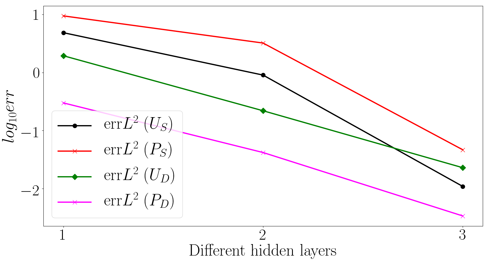
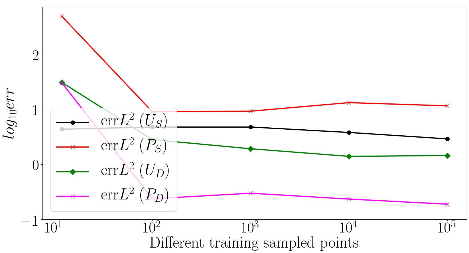
Similar to [47], we fix 𝐊\mathbf{K} to be the identity tensor in ℝ2×2,μ=ρ=β=ν=1\mathbb{R}^{2\times 2},~\mu=\rho=\beta=\nu=1. Due to the interface conditions (8) and (9) are violated, we exploit the interface conditions (55) and (56), where g1g_{1} and g2g_{2} can be computed by the exact solution. Specifically, the errors converge as the hidden layer increases in Figure 3(a). Figure 3(b) reveals that the change of data has no significant influence on errors once the size is larger than 10210^{2}. In particular, Figures 4 - 5 and Table 1 show the details of the results, this is consistent with our theory.
Refer to caption
(a) 400 training points
Refer to caption
(b) one hidden layer
Figure 3: The influence of different hidden layers and different training data on errL2L^{2} (Test 1).
Table 1: The relative errors of Test 1.
400 sampled points
1 layer 𝐔S\mathbf{U}_{S} PSP_{S} 𝐔D\mathbf{U}_{D} PDP_{D}
e​r​r​L1errL^{1} 2.49×1002.49\times 10^{0} 9.15×1009.15\times 10^{0} 8.72×1008.72\times 10^{0} 2.74×10−12.74\times 10^{-1}
e​r​r​L2errL^{2} 4.84×1004.84\times 10^{0} 9.42×1009.42\times 10^{0} 1.94×1001.94\times 10^{0} 2.99×10−12.99\times 10^{-1}
2 layers 𝐔S\mathbf{U}_{S} PSP_{S} 𝐔D\mathbf{U}_{D} PDP_{D}
e​r​r​L1errL^{1} 4.85×10−14.85\times 10^{-1} 3.59×1003.59\times 10^{0} 9.62×10−29.62\times 10^{-2} 4.03×10−24.03\times 10^{-2}
e​r​r​L2errL^{2} 9.01×10−19.01\times 10^{-1} 3.21×1003.21\times 10^{0} 2.19×10−12.19\times 10^{-1} 4.18×10−24.18\times 10^{-2}
3 layers 𝐔S\mathbf{U}_{S} PSP_{S} 𝐔D\mathbf{U}_{D} PDP_{D}
e​r​r​L1errL^{1} 5.80×10−35.80\times 10^{-3} 5.26×10−25.26\times 10^{-2} 1.01×10−21.01\times 10^{-2} 3.25×10−33.25\times 10^{-3}
e​r​r​L2errL^{2} 1.09×10−21.09\times 10^{-2} 4.66×10−24.66\times 10^{-2} 2.29×10−22.29\times 10^{-2} 3.38×10−33.38\times 10^{-3}
Refer to caption
Figure 4: The contrast of the exact solution and the CDNNs (Test 1).
Refer to caption
Figure 5: The point-wise errors (Test 1).

4.2 Test 2

In this example, we consider ΩS=(0,1)2,ΩD=(0,1)×(1,2)\Omega_{S}=(0,1)^{2},~\Omega_{D}=(0,1)\times(1,2) and the interface Γ={0<x<1,y=1}\Gamma=\{0<x<1,~y=1\} with an analytical solution presented in [47]. We set 𝐊\mathbf{K} to be the identity tensor in ℝ2×2,μ=ρ=β=ν=1\mathbb{R}^{2\times 2},~\mu=\rho=\beta=\nu=1, and the exact solution is given by

𝐮S=(−c​o​s2​(π​y2)​s​i​n​(π​x2)14​c​o​s​(π​x2)​(s​i​n​(π​y)+π​y)),pS=π4​c​o​s​(π​x2)​(y−2​c​o​s​(π​y2)2)\mathbf{u}_{S}=\left(\begin{array}[]{c}-cos^{2}(\frac{\pi y}{2})sin(\frac{\pi x}{2})\\ \frac{1}{4}cos(\frac{\pi x}{2})(sin(\pi y)+\pi y)\\ \end{array}\right),~~p_{S}=\frac{\pi}{4}cos(\frac{\pi x}{2})(y-2cos(\frac{\pi y}{2})^{2})

and

𝐮D=(−18​s​i​n​(π​x2)14​π​c​o​s​(π​x2)),pD=−π4​c​o​s​(π​x2)​y.\mathbf{u}_{D}=\left(\begin{array}[]{c}-\frac{1}{8}sin(\frac{\pi x}{2})\\ \frac{1}{4}\pi cos(\frac{\pi x}{2})\\ \end{array}\right),~~p_{D}=-\frac{\pi}{4}cos(\frac{\pi x}{2})y.
Table 2: The relative errors of Test 2.
400 sampled points
1 layer 𝐔S\mathbf{U}_{S} PSP_{S} 𝐔D\mathbf{U}_{D} PDP_{D}
e​r​r​L1errL^{1} 1.82×10−21.82\times 10^{-2} 1.19×10−11.19\times 10^{-1} 1.57×10−21.57\times 10^{-2} 1.08×10−21.08\times 10^{-2}
e​r​r​L2errL^{2} 3.66×10−23.66\times 10^{-2} 1.23×10−11.23\times 10^{-1} 4.62×10−24.62\times 10^{-2} 1.11×10−21.11\times 10^{-2}
2 layers 𝐔S\mathbf{U}_{S} PSP_{S} 𝐔D\mathbf{U}_{D} PDP_{D}
e​r​r​L1errL^{1} 2.27×10−42.27\times 10^{-4} 1.74×10−31.74\times 10^{-3} 1.04×10−41.04\times 10^{-4} 4.67×10−54.67\times 10^{-5}
e​r​r​L2errL^{2} 4.21×10−44.21\times 10^{-4} 2.00×10−32.00\times 10^{-3} 3.18×10−43.18\times 10^{-4} 5.55×10−55.55\times 10^{-5}
3 layers 𝐔S\mathbf{U}_{S} PSP_{S} 𝐔D\mathbf{U}_{D} PDP_{D}
e​r​r​L1errL^{1} 1.65×10−41.65\times 10^{-4} 1.01×10−31.01\times 10^{-3} 1.13×10−41.13\times 10^{-4} 7.69×10−57.69\times 10^{-5}
e​r​r​L2errL^{2} 3.37×10−43.37\times 10^{-4} 1.50×10−31.50\times 10^{-3} 3.44×10−43.44\times 10^{-4} 8.32×10−58.32\times 10^{-5}

Naturally, the corresponding 𝐟S,fD\mathbf{f}_{S},~f_{D}, and 𝐠D\mathbf{g}_{D} can be calculated by the exact solution. Note that this example satisfies the interface conditions (7) - (9). According to Test 1, we choose appropriate data and hidden layer to solve the second example. Figures 6 - 7 and Table 2 show the accuracy of the CDNNs for solving the coupled problems in detail.

Refer to caption
Figure 6: The contrast of the exact solution and the results of the CDNNs (Test 2).
Refer to caption
Figure 7: The point-wise errors (Test 2).

4.3 Test 3

In this subsection, we solve coupling of the Stokes and Darcy-Forchheimer problems with highly oscillatory permeability over domains ΩS=(0,1)×(0,1/2),ΩD=(0,1)×(1/2,1)\Omega_{S}=(0,1)\times(0,1/2),~\Omega_{D}=(0,1)\times(1/2,1) and the interface Γ={0<x<1,y=1/2}\Gamma=\{0<x<1,~y=1/2\} presented in [47]. Here we set μ=ρ=β=ν=1\mu=\rho=\beta=\nu=1, K−1=ϱ​IK^{-1}=\varrho I and ϱ\varrho is defined by

ϱ=2+1.8​s​i​n​(2​π​x/ε)2+1.8​s​i​n​(2​π​y/ε)+2+1.8​s​i​n​(2​π​y/ε)2+1.8​s​i​n​(2​π​x/ε),\varrho=\frac{2+1.8sin(2\pi x/\varepsilon)}{2+1.8sin(2\pi y/\varepsilon)}+\frac{2+1.8sin(2\pi y/\varepsilon)}{2+1.8sin(2\pi x/\varepsilon)},

where ε=1/16\varepsilon=1/16. The profile of ϱ\varrho is shown in Figure 8. The exact solution is given by

𝐮S=(16​y​c​o​s​(π​x)2​(y2−0.25)8​π​c​o​s​(π​x)​s​i​n​(π​x)​(y2−0.25)2),pS=x2\mathbf{u}_{S}=\left(\begin{array}[]{c}16ycos(\pi x)^{2}(y^{2}-0.25)\\ 8\pi cos(\pi x)sin(\pi x)(y^{2}-0.25)^{2}\\ \end{array}\right),~~p_{S}=x^{2}

and

𝐮D=(s​i​n​(2​π​x)​c​o​s​(2​π​y)−c​o​s​(2​π​x)​s​i​n​(2​π​y)),pD=c​o​s​(2​π​x)​c​o​s​(2​π​y).\mathbf{u}_{D}=\left(\begin{array}[]{c}sin(2\pi x)cos(2\pi y)\\ -cos(2\pi x)sin(2\pi y)\\ \end{array}\right),~~p_{D}=cos(2\pi x)cos(2\pi y).

We calculate the relative errors in Table 3 to reflect ability of the CDNNs for solving the coupled problems with highly oscillatory permeability. Figures 9 - 10 reveal that the CDNNs handle the highly oscillatory permeability coupled problems without losing accuracy.

Refer to caption
Figure 8: The value of ϱ\varrho (Test 3).
Table 3: The relative errors of Test 3.
400 sampled points
1 layer 𝐔S\mathbf{U}_{S} PSP_{S} 𝐔D\mathbf{U}_{D} PDP_{D}
e​r​r​L1errL^{1} 3.59×10−13.59\times 10^{-1} 5.03×1005.03\times 10^{0} 5.52×10−25.52\times 10^{-2} 7.59×10−27.59\times 10^{-2}
e​r​r​L2errL^{2} 6.79×10−16.79\times 10^{-1} 5.20×1005.20\times 10^{0} 1.73×10−11.73\times 10^{-1} 7.07×10−27.07\times 10^{-2}
2 layers 𝐔S\mathbf{U}_{S} PSP_{S} 𝐔D\mathbf{U}_{D} PDP_{D}
e​r​r​L1errL^{1} 8.42×10−48.42\times 10^{-4} 9.41×10−39.41\times 10^{-3} 1.15×10−31.15\times 10^{-3} 1.32×10−31.32\times 10^{-3}
e​r​r​L2errL^{2} 1.65×10−31.65\times 10^{-3} 1.05×10−21.05\times 10^{-2} 3.43×10−33.43\times 10^{-3} 1.56×10−31.56\times 10^{-3}
3 layers 𝐔S\mathbf{U}_{S} PSP_{S} 𝐔D\mathbf{U}_{D} PDP_{D}
e​r​r​L1errL^{1} 1.89×10−41.89\times 10^{-4} 3.04×10−33.04\times 10^{-3} 2.97×10−42.97\times 10^{-4} 6.70×10−56.70\times 10^{-5}
e​r​r​L2errL^{2} 3.65×10−43.65\times 10^{-4} 3.37×10−33.37\times 10^{-3} 8.98×10−48.98\times 10^{-4} 8.40×10−58.40\times 10^{-5}
Refer to caption
Figure 9: The contrast of the exact solution and the results of the CDNNs (Test 3).
Refer to caption
Figure 10: The point-wise errors (Test 3).

4.4 Test 4

The problems that we have studied so far have the exact solution. In this example, we consider coupling of the Stokes and Darcy-Forchheimer problems with no exact solution over ΩS=(−1/2,3/2)×(0,2),ΩD=(−1/2,3/2)×(−2,0)\Omega_{S}=(-1/2,3/2)\times(0,2),~\Omega_{D}=(-1/2,3/2)\times(-2,0) and the interface Γ={−1/2<x<3/2,y=0}\Gamma=\{-1/2<x<3/2,~y=0\}. Specifically, in the Stokes region, the Dirichlet boundary condition is given by Kovasznay flow [48],

𝐮S=(1−eλ​x​c​o​s​(2​π​y)λ2​π​eλ​x​s​i​n​(2​π​y)),\mathbf{u}_{S}=\left(\begin{array}[]{c}1-e^{\lambda x}cos(2\pi y)\\ \frac{\lambda}{2\pi}e^{\lambda x}sin(2\pi y)\\ \end{array}\right),

where λ=−8​π21+1+64​π2\lambda=\frac{-8\pi^{2}}{1+\sqrt{1+64\pi^{2}}}. Moreover, we set μ=ρ=β=ν=1\mu=\rho=\beta=\nu=1 and 𝐠D=𝟎,fD=0,𝐟S=𝟎\mathbf{g}_{D}=\mathbf{0},~f_{D}=0,~\mathbf{f}_{S}=\mathbf{0}. In addition, pDp_{D} satisfies the homogeneous Dirichlet boundary condition along y=−2y=-2, otherwise it has an homogeneous Neumann boundary condition. The permeability is taken to be K=ε​IK=\varepsilon I and the ε=104\varepsilon=10^{4}. Since the exact solution for this example is not available, we provide L2L^{2} error of interface to demonstrate the accuracy of the CDNNs in Table 4. Obviously, the error decreases gradually with the increasing of the hidden layers. Furthermore, Figures 11 - 12 display the exact solution and the results of CDNNs in detail.

Table 4: The error in interface of Test 4 (K=10000).
400 sampled points
I​n​t​e​r​f​a​c​e​1Interface1 I​n​t​e​r​f​a​c​e​2Interface2 I​n​t​e​r​f​a​c​e​3Interface3
1​l​a​y​e​r1~layer 6.49×10−26.49\times 10^{-2} 9.14×10−29.14\times 10^{-2} 3.03×10−23.03\times 10^{-2}
2​l​a​y​e​r​s2~layers 2.31×10−22.31\times 10^{-2} 4.74×10−24.74\times 10^{-2} 2.38×10−32.38\times 10^{-3}
3​l​a​y​e​r​s3~layers 2.12×10−22.12\times 10^{-2} 1.28×10−21.28\times 10^{-2} 4.94×10−44.94\times 10^{-4}
Refer to caption
Figure 11: The results of CDNNs (Test 4).
Refer to caption
(a) Stokes velocity.
Refer to caption
(b) Darcy velocity.
Figure 12: The velocity of Stokes and Darcy (Test 4).

4.5 Test 5

We conclude this section with a physical flow, where ΩS=(0,1)×(1,2),ΩD=(0,1)2\Omega_{S}=(0,1)\times(1,2),~\Omega_{D}=(0,1)^{2} and the interface Γ={0<x<1,y=1}\Gamma=\{0<x<1,~y=1\}. In ΩS\Omega_{S}, the boundaries of the cavity are walls with no-slip condition, except for the upper boundary where a uniform tangential velocity 𝐮S​(x,2)=(1,0)T\mathbf{u}_{S}(x,2)=(1,0)^{T} is imposed, which is driven cavity flow. And more precisely, we enforce homogeneous Neumann and Dirichlet boundary conditions, respectively, on ΓD,N={x=0ory=0}\Gamma_{D,N}=\{x=0~or~y=0\} and ΓD,D={x=1}\Gamma_{D,D}=\{x=1\}. In addition, we set KK to be the identity tensor in ℝ2×2,μ=ρ=β=ν=1\mathbb{R}^{2\times 2},~\mu=\rho=\beta=\nu=1, and fD=0,𝐟S=𝟎,𝐠D=𝟎f_{D}=0,~\mathbf{f}_{S}=\mathbf{0},~\mathbf{g}_{D}=\mathbf{0}. The results of the CDNNs are depicted in Figure 13. More vividly, we display the velocity flows of free-flow and porous media zones in Figure 13.

Refer to caption
Figure 13: The results of the CDNNs (Test 5).
Refer to caption
(a) Stokes velocity.
Refer to caption
(b) Darcy velocity.
Figure 14: The velocity flows of Stokes and Darcy (Test 5).

5 Conclusions

In this article, we proposed the CDNNs to study the coupled Stokes and Darcy-Forchheimer problems. This method can avoid many limitations of the traditional methods, such as decoupling, grid construction and the complicated interface conditions. Specially, we provide the convergence of the loss function and the convergence of the CDNNs to the exact solution. The numerical results are consistent with our theory sufficiently. Moreover, we leave the following issues subject to our future works, 1) Combining data-driven with model-driven to solve the high dimensional coupled problems; 2) Considering the specific size of the networks through theoretical analysis; 3) Combining traditional numerical methods with deep learning to solve more complicated high dimensional coupled problems.

References

  • [1] P. G. Saffman, On the boundary condition at the surface of a porous medium[J], Studies in Applied Mathematics, 1971 (50): 93-101.
  • [2] P. Forchheimer, Wasserbewegung durch Boden[J], Zeitz Vereines Deutsch Ingenieure, 1901 (45): 1782-1788.
  • [3] E. J. Park, Mixed finite element methods for nonlinear second order elliptic problems[J], SIAM Journal on Numerical Analysis, 1995 (32): 865-885.
  • [4] M. Y. Kim and E. J. park, Fully discrete mixed finite element approximations for non-Darcy flows in porous media[J], Computers and Mathematics with Applications, 1999 (38): 113-129.
  • [5] E. J. Park, Mixed finite element methods for generalized Forchheimer flow in porous media[J], Numerical Methods for Partial Differential Equations, 2005 (21): 213-228.
  • [6] M. Discacciati, E. Miglio, and A. Quarteroni, Mathematical and numerical models for coupling surface and groundwater flows[J], Applied Numerical Mathematics, 2002 (43): 57-74.
  • [7] W. J. Layton, F. Schieweck, and I. Yotov, Coupling fluid flow with porous media flow[J], SIAM Journal on Numerical Analysis, 2003 (40): 2195-2218.
  • [8] B. Rivie`\grave{e}re , Analysis of a discontinuous finite element method for the coupled Stokes and Darcy problems[J], Journal of Scientific Computing, 2005 (22): 479-500.
  • [9] B. Rivie`\grave{e}re and I. Yotov, Locally conservative coupling of Stokes and Darcy flows[J], SIAM Journal on Numerical Analysis, 2005 (42): 1959–1977.
  • [10] E. Burman and P. Hansbo, A unified stabilized method for Stokes’ and Darcy’s equations[J], Journal of Computational and Applied Mathematics, 2007 (198): 35-51.
  • [11] G. N. Gatica, R. Oyarzu´\acute{u}a, and F. J. Sayas, Analysis of fully mixed finite element methods for the Stokes-Darcy coupled problem[J], Mathematics of Computation, 2001 (80): 1911-1948.
  • [12] V. Girault, D. Vassilev, and I. Yotov, Mortar multiscale finite element methods for StokesDarcy flows[J], Numerische Mathematik, 2014 (127): 93-165.
  • [13] K. Lipnikov, D. Vassilev, and I. Yotov, Discontinuous Galerkin and mimetic finite difference methods for coupled Stokes-Darcy flows on polygonal and polyhedral grids[J], Numerische Mathematik, 2014 (126): 321-360.
  • [14] A. Krizhevsky, I. Sutskever, G.E. Hinton, Imagenet classification with deep convolutional neural networks[J], Advances in Neural Information Processing Systems. 2012: 1097-1105.
  • [15] G. Hinton, L. Deng, D. Yu, G.E. Dahl, A. rahman Mohamed, N. Jaitly, A. Senior, Approximation capabilities of multilayer feedforward networks[J], IEEE Signal Processing Magazine. 2012 (29): 82-97.
  • [16] K. He, X. Zhang, S. Ren, J. Sun, Deep residual learning for image recognition[J], Proceedings of the IEEE Conference on Computer Vision and Pattern Recognition, 2016: 770-778.
  • [17] N. E. Cotter, The Stone-Weierstrass theorem and its application to neural networks[J]. IEEE Transaction on Neural Networks. 1990, 1 (4): 290-295.
  • [18] K. Hornik, M. Stinchcombe and H. White, Multilayer feedforward networks are universal approximators[J]. Neural Networks. 1989, 2 (5): 359-366.
  • [19] K. Hornik, M. Stinchcombe and H. White, Universal approximation of an unknown mapping and its derivatives using multilayer feedforward networks[J]. Neural Networks. 1990: 3(5): 551-560.
  • [20] K. Hornik, Approximation capabilities of multilayer feedforward networks[J], Neural Networks. 1991 (4): 251-257.
  • [21] G. Cybenko, Approximations by superpositions of sigmoidal functions[J], Mathematics of Control, Signals, and Systems. 1989 (2): 303-314.
  • [22] B. C. Csa´\acute{a}ji, Approximation With Artificial Neural Networks[M], Faculty of Sciences, Eo¨\ddot{o}tvo¨\ddot{o}s Lora´\acute{a}nd University, 2001.
  • [23] M. Telgrasky, Benefits of depth in neural networks[J], Journal of Machine Learning Research: Workshop and Conference Proceedings. 2016 (49): 1-23.
  • [24] H. M. Q. Liao, T. Poggio, Learning functions: when is deep better than shallow[J], arXiv preprint arXiv:1603.00988v4, 2016. [Online]. Available: https://arxiv.org/abs/1603.00988.
  • [25] Y. Khoo, J. Lu, L. Ying, Solving parametric PDE problems with artificial neural networks[J], arXiv preprint arXiv:1707.03351, 2017. [Online]. Available: https://arxiv.org/abs/1707.03351.
  • [26] J. Li, J. Yue, W. Zhang, W. Duan, The Deep Learning Galerkin Method for the General Stokes Equations[J]. arXiv preprint arXiv:2009.11701, 2020. [Online]. Available: https://arxiv.org/abs/2009.11701.
  • [27] J. Li, W. Zhang and J. Yue, A Deep Learnign Galerkin Method for the Second-order linear elliptic equations[J]. International Journal of Numerical Analysis and Modeling. 2021, 18(4): 427-441.
  • [28] J. Yue, J. Li, The Deep Learning Galerkin Method for the unsteady Stokes Equations[J]. Journal of Computational Physics. Under review.
  • [29] Y. Fan, L. Lin, L. Ying, L. Zepeda-Nu´\acute{u}nez, A multiscale neural network based on hierarchical matrices[J], arXiv preprint arXiv:1807.01883, 2018. [Online]. Available: https://arxiv.org/abs/1807.01883.
  • [30] M. Wang , S. W. Cheung, E. T. Chung, et al. , Prediction of discretization of gmsfem using deep learning[J], arXiv preprint arXiv: 1810.12245, 2018. [Online]. Available: https://arxiv.org/abs/1810.12245.
  • [31] X. Li, Simultaneous approximations of multivariate functions and their derivatives by neural networks with one hidden layer[J]. Neurocomputing. 1996, 12(4): 327-343.
  • [32] I. E. Lagaris, A. C. Likas and D. I. Fotiadis, Artificial neural networks for solving ordinary and partial differential equations[J]. IEEE Transaction on Neural Networks. 1998, 9(5): 987-1000.
  • [33] I. E. Lagaris, A. C. Likas and D. G. Papageorgiou, Neural-network methods for boundary value problems with irregular boundaries[J]. IEEE Transaction on Neural Networks. 2000, 11(5): 1041-1049.
  • [34] K. S. McFall and J. R. Mahan, Artificial neural network method for solution of boundary value problems with exact satisfaction of arbitrary boundary conditions[J]. IEEE Transaction on Neural Networks. 2009, 20(8): 1221-1233.
  • [35] M. Raissi, P. Perdikaris and G. E. Karniadakis, Physics informed deep learning (Part I): Data-driven solutions of nonlinear partial differential equations[J]. 2017, arXiv:1711.10561. [Online]. Available: https://arxiv.org/abs/1711.10561.
  • [36] M. Raissi, P. Perdikaris and G. E. Karniadakis, Physics informed deep learning (Part II): Data-driven discovery of nonlinear partial differential equations[J]. 2017, arXiv:1711.10566. [Online]. Available: https://arxiv.org/abs/1711.10566.
  • [37] M. Raissi, P. Perdikaris and G. E. Karniadakis, Physics-informed neural networks: A deep learning framework for solving forward and inverse problems involving nonlinear partial differential equations[J]. Journal of Computational Physics. 2019 (378): 686-707.
  • [38] L. Yang, X. Meng, G. E. Karniadakis, B-PINNs: Bayesian Physics-Informed Neural Networks for Forward and Inverse PDE Problems with Noisy Data[J]. Journal of Computational Physics. 2021 (425): 109913.
  • [39] C. Rao, H. Sun and Y. Liu, Physics informed deep learning for computational elastodynamics without labeled data[J]. arXiv: 2006.08472v1. 2020. [Online]. Available: https://arxiv.org/abs/2006.08472.
  • [40] P. Olivier and R. Fablet. PDE-NetGen 1.0: from symbolic PDE representations of physical processes to trainable neural network representations[J]. arXiv:2002.01029. [Online]. Available: https://arxiv.org/abs/2002.01029 2020.
  • [41] L. Lu, X. Meng, Z. Mao and G. E. Karniadakis, DEEPXDE: A Deep Learning Library for solving differencial equations[J]. SIAM Review. 63(1), 208-228.
  • [42] Z. Fang and J. Zhan, A Physics-Informed Neural Network Framework for PDEs on 3D Surfaces: Time Independent Problems[J]. IEEE Access. 2020 (8): 26328-26335.
  • [43] G. Pang, L. Lu and G. E. Karniadakis, fPINNs: Fractional Physics-Informed Neural Networks[J]. SIAM Journal on Scientific Computing. 2018, 41(4): A2603-A2626.
  • [44] Y. Zhu, N. Zabaras, P.-S. Koutsourelakis, P. Perdikaris, Physics-constrained deep learning for high-dimensional surrogate modeling and uncertainty quantification without labeled data[J], Journal of Computational Physics. 2019 (394): 56-81.
  • [45] J. Sirignano and K. Spiliopoulos, DGM: A deep learning algorithm for solving partial differential equations[J]. Journal of Computational Physics. 2018 (375): 1339-1364.
  • [46] G. S. Beaver and D. D. Joseph, Boundary conditions at a naturally imperable wall[J], Journal of Fluid Mechanics, 1967 (30): 197-207.
  • [47] Zhao L., Chung E., Park E. J., et al. Staggered DG method for coupling of the Stokes and Darcy-Forchheimer problems[J]. SIAM Journal on Numerical Analysis. 2019, 59(1): 1-31.
  • [48] L. I. G. Kovasznay, Laminar flow behind a two-dimension grid[J], Mathematical Proceedings of the Cambridge Philosophical Society, 1948 (44): 58-62.
  • [49] Le´\acute{e}on Bottou: Stochastic Gradient Tricks, Neural Networks, Tricks of the Trade, Reloaded, 430-445, Edited by Gre´\acute{e}goire Montavon, Genevieve B. Orr and Klaus-Robert Mu¨\ddot{u}ller, Lecture Notes in Computer Science (LNCS 7700), Springer, 2012.