Dynamical Mean-Field Theory for spin-dependent electron transport in spin-valve devices

The typical system that we consider is shown schematically in Fig. 1 and represents a two-terminal device. The transport direction is along the $z$ Cartesian axis. We employ a linear combination of atomic orbitals (LCAO) basis set. The system is divided in three parts: a central region (CR) and left ($L$) and right ($R$) electrodes, from which electrons flow in and out. To start with, we assume that electrons in both the CR and the electrodes are effectively non-interacting. Each electrode is semi-infinite and periodic away from the CR; $\mathbf{k}=(k_{x},k_{y})$ indicates the wave-vector in the transverse direction. $H^{\sigma}(\mathbf{k})$ is the $\mathbf{k}$-dependent single-particle Hamiltonian of the CR for electrons of spin $\sigma=\uparrow,\downarrow$. Note that we assume that there are no spin-mixing terms in the Hamiltonian. Since in general the basis set is non-orthogonal, there is also a spin-independent orbital overlap $S(\mathbf{k})$ of the CR. We denote with $N$ the number of basis orbitals of the CR. $H^{\sigma}(\mathbf{k})$ and $S(\mathbf{k})$ are therefore matrices of dimension $N\times N$. Each electrode is in local thermal equilibrium at its own chemical potential $\mu_{L/R}$ due to its infinitely large size. When there is no applied bias voltage across the electrodes, we have $\mu_{L}=\mu_{R}=E_{F}$, where $E_{F}$ the Fermi energy. When a finite bias voltage $V$ is applied, the chemical potentials are shifted as $\mu_{L/R}=E_{F}\pm eV/2$, where $e$ is the electron charge.
To describe the electronic structure and the quantum transport properties of the device, we use the non-equilibrium Green’s function (NEGF) approachDatta 1995. The effect of electrodes on the CR is then captured via the momentum- and energy-dependent retarded electrode self-energies, $\Sigma^{\sigma}_{L}(\mathbf{k},E)$ and $\Sigma^{\sigma}_{R}(\mathbf{k},E)$. Their antihermitian parts

$$\Gamma^{\sigma}_{L/R}(\mathbf{k},E)=i[\Sigma^{\sigma}_{L/R}(\mathbf{k},E)-\Sigma^{\sigma}_{L/R}(\mathbf{k},E)^{\dagger}]$$

(1)

represent the strength of the electronic coupling between the electrodes and the CR. The properties of the CR are then fully described by the retarded and lesser CR Green’s functions, defined as

$$g^{\sigma}(\mathbf{k},E)=[ES(\mathbf{k})-H^{\sigma}(\mathbf{k})-\Sigma^{\sigma}_{L}(\mathbf{k},E)-\Sigma^{\sigma}_{R}(\mathbf{k},E)]^{-1},$$

(2)

$$g^{\sigma<}(\mathbf{k},E)=g^{\sigma}(\mathbf{k},E)[\Sigma^{\sigma<}_{L}(\mathbf{k},E)+\Sigma^{\sigma<}_{R}(\mathbf{k},E)]g^{\sigma}(\mathbf{k},E)^{\dagger},$$

(3)

where the lesser electrodes’ self-energies are

$$\Sigma^{\sigma<}_{L(R)}(\mathbf{k},E)=if_{L(R)}(E)\Gamma^{\sigma}_{L(R)}(\mathbf{k},E),$$

(4)

with $f_{L/R}(E)=[e^{\beta(E-\mu_{L/R})}+1]^{-1}$ the Fermi function of the left/right electrode; here $\beta=1/k_{\mathrm{B}}\theta$, with $k_{\mathrm{B}}$ representing the Boltzmann constant, and $\theta$ the electronic temperature. The Green’s functions of the CR and the self-energies are $N\times N$ matrices like $H^{\sigma}(\mathbf{k})$.
The density matrix of the CR is given by

$$\rho^{\sigma}=\frac{1}{N_{\mathbf{k}}}\sum_{\mathbf{k}}\bigg[\frac{1}{2\pi i}\int dE\;g^{\sigma<}(\mathbf{k},E)\bigg]$$

(5)

where $N_{\mathbf{k}}$ is the number of $\mathbf{k}$-points in the Brillouin zone. In our calculations, $H^{\sigma}(\mathbf{k})$ is the DFT Kohn-Sham Hamiltonian within the LSDA, and it is therefore density dependent. Eqs. (2), (3) and (5) need to be evaluated self-consistently Brandbyge et al. 2002; Rocha et al. 2006; Rungger et al. 2019. This method is usually called DFT+NEGF, and it is the state-of-the-art approach to study spin-dependent transport through nano-devices. Here, we use the implementation of DFT+NEGF in the Smeagol transport codeRocha et al. 2006; Rungger and Sanvito 2008, which obtains the LSDA Kohn-Sham Hamiltonian from the DFT package SiestaSoler et al. 2002.
The current across the CR for electrons of spin $\sigma$ is evaluated asDatta 1995; Brandbyge et al. 2002; Rocha et al. 2006; Rungger et al. 2019

$$I=\frac{e}{h}\sum_{\sigma}\int T^{\sigma}(E)[f_{L}(E)-f_{R}(E)]dE,$$

(6)

where $h$ is Planck’s constant, and

	$\displaystyle T^{\sigma}(E)=\frac{1}{N_{\mathbf{k}}}\sum_{\mathbf{k}}T^{\sigma}(\mathbf{k},E),$		(7)
	$\displaystyle T^{\sigma}(\mathbf{k},E)=\mathrm{Tr}\Big[\Gamma^{\sigma}_{L}(\mathbf{k},E)g^{\sigma}(\mathbf{k},E)^{\dagger}\Gamma^{\sigma}_{R}(\mathbf{k},E)g^{\sigma}(\mathbf{k},E)\Big]$

is the spin- and energy-dependent transmission coefficient. The device conductance is finally defined as $\mathfrak{G}=dI/dV$.
The approach described so far is general and can be applied to any electronic system. However, in the rest of this paper, our focus will be on metallic heterostructures. Because of electronic screening, there can be no bias voltage drop across the electrodes. Therefore, we take the linear-response limit, also denoted as zero-bias limit, $\mu_{L}-\mu_{R}\rightarrow 0$. At zero temperature ($\theta=0$) the conductance reduces to the well-known Landauer formula

$$\mathfrak{G}=\frac{\mathfrak{G}_{0}}{2}\sum_{\sigma}T^{\sigma}(E_{F}),$$

(8)

where $\mathfrak{G}_{0}=2e^{2}/h$ is the quantum of conductance. Notably, for non-interacting electrons, the Landauer and the so-called Kubo approaches are equivalentBaranger and Stone 1989; Fisher and Lee 1981, so that the linear-response transport properties of a system can be computed by either approach.

The described NEGF method for transport is formally extended beyond the effective single-particle picture by adding the many-body retarded and lesser self-energies, $\Sigma^{\sigma}_{MB}(\mathbf{k},E)$ and $\Sigma^{\sigma<}_{MB}(\mathbf{k},E)$ to Eqs. (2) and (3) (see, for example, Ref. Stefanucci and van Leeuwen 2013). Thus the Green’s functions of the CR with interacting electrons becomeFerretti et al. 2005a; Ferretti et al. 2005b; Thygesen and Rubio 2008

$$\begin{split}G^{\sigma}(\mathbf{k},E)=&[ES(\mathbf{k})-H^{\sigma}(\mathbf{k})-\Sigma^{\sigma}_{L}(\mathbf{k},E)-\Sigma^{\sigma}_{R}(\mathbf{k},E)\\ &-\Sigma^{\sigma}_{MB}(\mathbf{k},E)]^{-1},\end{split}$$

(9)

and

$$\begin{split}G^{\sigma<}(\mathbf{k},E)=&G^{\sigma}(\mathbf{k},E)[\Sigma^{\sigma<}_{L}(\mathbf{k},E)+\Sigma^{\sigma<}_{R}(\mathbf{k},E)\\ &+\Sigma^{\sigma<}_{MB}(\mathbf{k},E)]G^{\sigma}(\mathbf{k},E)^{\dagger}.\end{split}$$

(10)

Eq. (9) can be re-expressed as a Dyson equation

$$G^{\sigma}(\mathbf{k},E)=g^{\sigma}(\mathbf{k},E)+g^{\sigma}(\mathbf{k},E)\Sigma^{\sigma}_{MB}(\mathbf{k},E)G^{\sigma}(\mathbf{k},E),$$

(11)

which allows to obtain the retarded many-body Green’s function, also called dressed Green’s function, from the non-interacting, or bare, Green’s function $g^{\sigma}(\mathbf{k},E)$ of Eq. (2).
The formal introduction of the many-body self-energies shows that the electron-electron interaction effectively acts on the system as an additional electrode. We can then define the effective “coupling” matrixDroghetti and Rungger 2017

$$\Gamma_{MB}^{\sigma}(\mathbf{k},E)=i[\Sigma^{\sigma}_{MB}(\mathbf{k},E)-\Sigma^{\sigma}_{MB}(\mathbf{k},E)^{\dagger}],$$

(12)

and express $\Sigma^{<}_{MB}(\mathbf{k},E)$ asDroghetti and Rungger 2017

$$\Sigma^{\sigma<}_{MB}(\mathbf{k},E)=iF^{\sigma}_{MB}(\mathbf{k},E)\Gamma^{\sigma}_{MB}(\mathbf{k},E).$$

(13)

This equation has the same structure as Eq. (4), but $F^{\sigma}_{MB}(\mathbf{k},E)$ is a matrix, which describes the out-of-equilibrium distribution of the interacting electrons in the CR, and it is not the Fermi function. The resulting current was first computed by Meir and Wingreen in a seminal workMeir and Wingreen 1992, and can be written asDroghetti and Rungger 2017

$$I=I_{c}+I_{nc}.$$

(14)

$I_{c}$ is the coherent contribution expressed as in Eq. (6), but with the transmission coefficient $T^{\sigma}(E)$ evaluated with the retarded dressed Green’s function, i.e., replacing $T^{\sigma}(\mathbf{k},E)$ with

$$T^{\sigma}_{MB}(\mathbf{k},E)=\mathrm{Tr}\Big[\Gamma^{\sigma}_{L}(\mathbf{k},E)G^{\sigma}(\mathbf{k},E)^{\dagger}\Gamma^{\sigma}_{R}(\mathbf{k},E)G^{\sigma}(\mathbf{k},E)\Big].$$

(15)

$I_{nc}$ is the non-coherent contribution, and readsNess et al. 2010; Droghetti and Rungger 2017

$$\begin{split}I_{nc}=&\sum_{\sigma}\mathrm{Tr}\Big\{[F^{\sigma}_{MB}(\mathbf{k},E)-f_{R}(E)]\times\\ &\Gamma^{\sigma}_{MB}(\mathbf{k},E)G^{\sigma}(\mathbf{k},E)^{\dagger}\Gamma^{\sigma}_{MB}(\mathbf{k},E)G^{\sigma}(\mathbf{k},E)\Big\}.\end{split}$$

(16)

It accounts for an effective “interaction electrode”. Electrons can be seen as entering the interaction electrode, where they undergo some scattering processes losing coherence, before being re-injected into the systemFörster et al. 2007. The mathematical form of $I_{nc}$ resembles that of $I_{c}$. However, $F^{\sigma}_{MB}(\mathbf{k},E)$ cannot be brought outside the trace, and $I_{nc}$ cannot be associated to a transmission coefficient for the flow of electrons from the interaction electrode Ness et al. 2010.
Given Eq. (14), the conductance $\mathfrak{G}$ can similarly be separated into a coherent and non-coherent contribution. In the linear-response limit relevant for metallic heterostructures, the calculation of such non-coherent contribution is however an outstanding problem. To date, it has only been solved assuming either a specific shape for the matrix $F^{\sigma}_{MB}(\mathbf{k},E)$ (Refs. Ferretti et al. 2005a; Ng 1996), or that the CR consists of a single orbital, so that $\Gamma^{\sigma}_{L/R}$ are numbers instead of matricesMeir and Wingreen 1992. Alternatively, in the Kubo formalism, non-coherent contributions would be captured by vertex correctionsOguri 2001, but we are not aware of any study, where these have been derived from first-principles calculations. Since the goal of our paper is not to provide a solution for this problem, but to present our implementation of LSDA+DMFT, we focus here on analysis of the transmission coefficient in Eq. (15) rather than on the conductance. Importantly, $T^{\sigma}_{MB}(\mathbf{k},E_{F})$ can be directly measured in experiment through the injection of hot electrons or holes in metallic heterostructuresAlekhin et al. 2017; Banerjee et al. 2005; Kaidatzis et al. 2008. Therefore, our calculations can provide physically relevant and verifiable predictions on correlation effects in quantum transport. This will be further discussed in Sec. IV.2.
In the zero-bias limit implied for metallic systems, $T^{\sigma}_{MB}(\mathbf{k},E_{F})$ is calculated with the retarded dressed Green’s function evaluated in thermodynamics equilibrium. The fluctuation-dissipation theorem holds, and givesStefanucci and van Leeuwen 2013

$$G^{\sigma<}(\mathbf{k},E)=if(E)D^{\sigma}(\mathbf{k},E),$$

(17)

where $f(E)=f_{L}(E)=f_{R}(E)$, and

$$D^{\sigma}(\mathbf{k},E)=i[G^{\sigma}(\mathbf{k},E)-G^{\sigma}(\mathbf{k},E)^{\dagger}]$$

(18)

is the spectral function. Thus, only $G^{\sigma}(\mathbf{k},E)$ is required to fully describe the system. In summary, solving the interacting problem and calculating the transport properties within the mentioned approximations reduce to the evaluation of the retarded self-energy $\Sigma^{\sigma}_{MB}(\mathbf{k},E)$ and of the Dyson equation, Eq. (11).

The discussion in the previous section provided formal equations to study transport in correlated nano-devices. However, calculations including all the orbitals of the CR represent a great challenge in practical calculations. To simplify the problem, we take advantage of the fact that in the case of TM-based heterostructures there are $4s$ and $3d$ valence states. $4s$ states are delocalized forming energy bands with a large dispersion, and electronic correlations are well described at the effective single-particle Kohn-Sham level. In contrast, open $3d$ shells are more tightly bound to the ionic cores, and, as such, they are moderately correlated. We then define the “correlated subspace” ($\mathcal{C}$) as the subspace of the CR that includes all $3d$ orbitals. Assuming that there are $N_{\mathrm{TM}}$ TM atoms inside the CR, the correlated subspace $\mathcal{C}$ has dimension $2(5\times N_{\mathrm{TM}})$ (the factor $2$ accounts for the spin). The correlated subspace can be projected out from the rest of the system, which we refer to as the “bath” (B), and which includes the orthogonal subspace to $\mathcal{C}$ within both the CR and electrodes. To carry out such projection, we use the scheme presented in Ref. Droghetti and Rungger 2017, and we perform the basis change, which transforms the CR overlap and Hamiltonian matrix as

$$\begin{split}\bar{S}(\mathbf{k})=\left(\begin{array}[]{cc}1&0\\ 0&\bar{S}_{\mathrm{B}}(\mathbf{k})\\ \end{array}\right)=\\ =W(\mathbf{k})^{\dagger}S(\mathbf{k})W(\mathbf{k}),\end{split}$$

(19)

$$\begin{split}\bar{H}^{\sigma}(\mathbf{k})=\left(\begin{array}[]{cc}\bar{H}^{\sigma}_{\mathcal{C}}(\mathbf{k})&\bar{H}^{\sigma}_{\mathcal{C},\mathrm{B}}(\mathbf{k})\\ \bar{H}^{\sigma}_{\mathrm{B},\mathcal{C}}(\mathbf{k})&\bar{H}^{\sigma}_{\mathrm{B}}(\mathbf{k})\\ \end{array}\right)=\\ =W(\mathbf{k})^{\dagger}H^{\sigma}(\mathbf{k})W(\mathbf{k}).\end{split}$$

(20)

In the transformed matrices $\bar{S}(\mathbf{k})$ and $\bar{H}^{\sigma}(\mathbf{k})$ the top left block describes the correlated subspace $\mathcal{C}$, the bottom right block describes the part of the bath included in the CR, and the off-diagonal blocks describe the connection terms. The matrices $W(\mathbf{k})$ are defined in Eq. (10) of Ref. Droghetti and Rungger 2017 . The transformation is designed in such a way that the orbitals of $\mathcal{C}$ become orthogonal, and that they have zero overlap with the bath orbitals [see Eq. (19)].
$\bar{H}^{\sigma}_{\mathcal{C}}(\mathbf{k})$ in Eq. (20) is the non-interacting Hamiltonian matrix of $\mathcal{C}$ of dimension $5N_{\mathrm{TM}}\times 5N_{\mathrm{TM}}$. Using the second quantization formalism, we can introduce the Hamiltonian operator of $\mathcal{C}$

$$\hat{\bar{H}}^{\sigma}_{\mathcal{C}}(\mathbf{k})=\sum_{i,j,\lambda_{1},\lambda_{2},\sigma}[\bar{H}^{\sigma}_{\mathcal{C}}(\mathbf{k})]_{i\lambda_{1},j\lambda_{2}}\hat{d}_{i\lambda_{1}\sigma}^{{\dagger}}\hat{d}_{j\lambda_{2}\sigma},$$

(21)

where $\hat{d}_{i\lambda\sigma}^{{\dagger}}$ and $\hat{d}_{i\lambda\sigma}$ are the electron creation and annihilation operators at orbital $\lambda$ within the atom $i$ and spin $\sigma$ ($i=1,...,N_{\mathrm{TM}}$ and $\lambda=1,...,5$, $\sigma=\uparrow,\downarrow$). $[\bar{H}^{\sigma}_{\mathcal{}}(\mathbf{k})]_{i\lambda_{1},j\lambda_{2}}$ is the Hamiltonian matrix element between the $d$ orbital $\lambda_{1}$ of the atom $i$ and the $d$ orbital $\lambda_{2}$ of the atom $j$. Further, to describe the electron-electron interaction for the electrons in $\mathcal{C}$, we add an explicit Coulomb term as follows

$$\begin{split}&\hat{\bar{H}}^{\sigma}(\mathbf{k})_{\mathcal{C},U}=\hat{\bar{H}}^{\sigma}_{\mathcal{C}}(\mathbf{k})-\hat{H}^{\sigma}_{\mathcal{C},dc}+\\ &+\frac{1}{2}\sum_{\begin{subarray}{c}i,\lambda_{1},\lambda_{2},\lambda_{3},\\ \lambda_{4},\sigma_{1},\sigma_{2}\end{subarray}}U_{\lambda_{1},\lambda_{2},\lambda_{3},\lambda_{4}}d_{i\lambda_{1}\sigma_{1}}^{{\dagger}}d_{i\lambda_{2}\sigma_{2}}^{{\dagger}}d_{i\lambda_{4}\sigma_{2}}d_{i\lambda_{3}\sigma_{1}},\end{split}$$

(22)

where $U_{\lambda_{1},\lambda_{2},\lambda_{3},\lambda_{4}}$ are the four-index Hubbard-$U$ matrix elements, which account for the screened Coulomb interaction between all $3d$ orbitals located on the same atom. $U_{\lambda_{1},\lambda_{2},\lambda_{3},\lambda_{4}}$ are parameterized in terms of the average effective Coulomb interaction $U$ and exchange $J$ (Ref. Pavarini 2011)

	$\displaystyle U=\frac{1}{(2l+1)^{2}}\sum_{\lambda_{1},\lambda_{2}}U_{\lambda_{1},\lambda_{2},\lambda_{1},\lambda_{2}}$		(23)
	$\displaystyle J=\frac{1}{2l(2l+1)}\sum_{\lambda_{1}\neq\lambda_{2},\lambda_{2}}U_{\lambda_{1},\lambda_{2},\lambda_{2},\lambda_{1}}.$		(24)

The reason for using the multi-orbital Hubbard-like form is the local nature of the screened Coulomb interaction, which allows us to ignore the Coulomb integrals involving correlated orbitals of different atoms. $\hat{H}^{\sigma}_{\mathcal{C},dc}$ is the double-counting correction, which is needed to cancel the Coulomb interactions already taken into account in the LSDA exchange-correlation potential. The exact form of the double-counting correction is not known, but several approximations have been proposed and are used in practice Lichtenstein et al. 2001; Kotliar et al. 2006; Karolak et al. 2010; Haule et al. 2010. We will describe our practical treatment of the problem in Secs. II.6 and II.7.
We note that taking the static mean-field approximation for the Hubbard-like interaction in the Hamiltonian of Eq. (22) leads to the so-called LSDA+$U$ methodAnisimov et al. 1991; Liechtenstein et al. 1995; Dudarev et al. 1998; Cococcioni and de Gironcoli 2005. This is one of the simplest corrective approaches that were formulated to improve the accuracy of LSDA functionals for correlated materials. We will further discuss it in Sec. II.6 and present some calculations in Appendix A. LSDA+$U$ has found widespread use for the computational design of functional materials. However, it was already shown in early worksCococcioni and de Gironcoli 2005 that it can give worse results than LSDA for the electronic spectra and, therefore, the transport properties of the ferromagnetic metallic systems of our interest. To obtained improved results, the Hubbard-like interaction in $\hat{\bar{H}}^{\sigma}(\mathbf{k})_{\mathcal{C},U}$ needs to be treated beyond the static mean-field approximation introducing a many-body energy-dependent self-energy as we will describe in the rest of the paper.

The bare and dressed Green’s functions, $g^{\sigma}(\mathbf{k},E)$ and $G^{\sigma}(\mathbf{k},E)$, are expressed in the transformed basis asDroghetti and Rungger 2017

$$\begin{split}\bar{g}^{\sigma}(\mathbf{k},E)=\left(\begin{array}[]{cc}\bar{g}^{\sigma}_{\mathcal{C}}(\mathbf{k},E)&\bar{g}^{\sigma}_{\mathrm{\mathcal{C},B}}(\mathbf{k},E)\\ \bar{g}^{\sigma}_{\mathrm{B,\mathcal{C}}}(\mathbf{k},E)&\bar{g}^{\sigma}_{\mathrm{B}}(\mathbf{k},E)\\ \end{array}\right)=\\ =W(\mathbf{k})^{-1}g^{\sigma}(\mathbf{k},E)W(\mathbf{k})^{-1\dagger}\end{split}$$

(25)

and

$$\begin{split}\bar{G}^{\sigma}(\mathbf{k},E)=\left(\begin{array}[]{cc}\bar{G}^{\sigma}_{\mathcal{C}}(\mathbf{k},E)&\bar{G}^{\sigma}_{\mathrm{\mathcal{C},B}}(\mathbf{k},E)\\ \bar{G}^{\sigma}_{\mathrm{B,\mathcal{C}}}(\mathbf{k},E)&\bar{G}^{\sigma}_{\mathrm{B}}(\mathbf{k},E)\\ \end{array}\right)=\\ =W(\mathbf{k})^{-1}G^{\sigma}(\mathbf{k},E)W(\mathbf{k})^{-1\dagger},\end{split}$$

(26)

where $W(\mathbf{k})^{-1}$ is the inverse of the transformation matrix used in Eqs. (19) and (20). $\bar{g}^{\sigma}(\mathbf{k},E)$ and $\bar{G}^{\sigma}(\mathbf{k},E)$ have the same block structure as the Hamiltonian matrix in Eq. (20). The blocks $\bar{g}^{\sigma}_{\mathcal{C}}(\mathbf{k},E)$ and $\bar{G}^{\sigma}_{\mathcal{C}}(\mathbf{k},E)$ are the bare and dressed Green’s function matrices of the correlated subspace. They satisfy the Dyson equation for the correlated subspace

$$\bar{G}^{\sigma}_{\mathcal{C}}(\mathbf{k},E)=[\bar{g}^{\sigma}_{\mathcal{C}}(\mathbf{k},E)^{-1}-\bar{\Sigma}^{\sigma}_{\mathcal{C}}(\mathbf{k},E)]^{-1},$$

(27)

where $\bar{\Sigma}^{\sigma}_{\mathcal{C}}(\mathbf{k},E)$ is the many-body self-energy of $\mathcal{C}$ and includes also the double counting correction. This self-energy formally specifies the electron correlations inside $\mathcal{C}$ due to the interaction in Eq. (22). In the following sections we will see how $\bar{\Sigma}^{\sigma}_{\mathcal{C}}(\mathbf{k},E)$ is computed in practice.
From $\bar{\Sigma}^{\sigma}_{\mathcal{C}}(\mathbf{k},E)$ we can easily obtain the many-body self-energy of whole CR. In the transformed basis, it reads

$$\bar{\Sigma}^{\sigma}_{MB}(\mathbf{k},E)=\left(\begin{array}[]{cc}\bar{\Sigma}^{\sigma}_{\mathcal{C}}(\mathbf{k},E)&0\\ 0&0\\ \end{array}\right),$$

(28)

since the bath is non-interacting by construction. In the original basis the CR many-body self-energy is calculated as

$$\Sigma^{\sigma}_{MB}(\mathbf{k},E)=W(\mathbf{k})^{-1^{\dagger}}\bar{\Sigma}^{\sigma}_{MB}(\mathbf{k},E)W(\mathbf{k})^{-1}.$$

(29)

The many-body self-energy is therefore “propagated” to the bath.

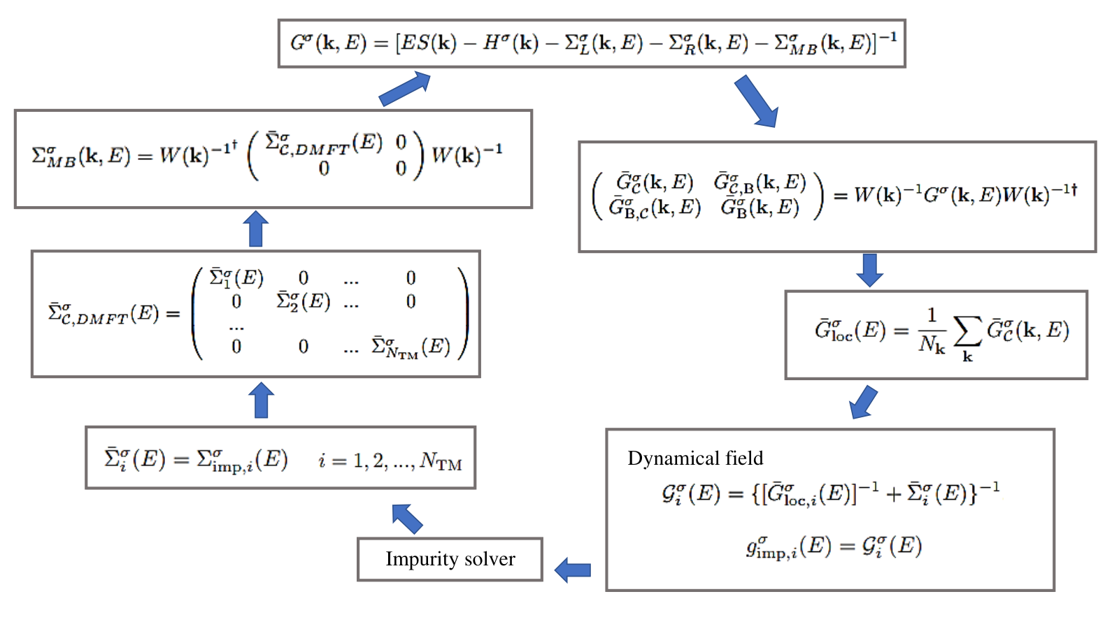
The many-body problem within the correlated subspace $\mathcal{C}$ is solved via DMFT, which means that we only consider electron correlations local in space. The self-energy $\bar{\Sigma}^{\sigma}_{\mathcal{C}}(\mathbf{k},E)$ of $\mathcal{C}$ is therefore approximated by the DMFT self-energy

$$\bar{\Sigma}^{\sigma}_{\mathcal{C},DMFT}(E)=\left(\begin{array}[]{cccc}\bar{\Sigma}^{\sigma}_{1}(E)&0&...&0\\ 0&\bar{\Sigma}^{\sigma}_{2}(E)&...&0\\ 0&0&...&\bar{\Sigma}^{\sigma}_{N_{\mathrm{TM}}}(E)\\ \end{array}\right),$$

(30)

where $\bar{\Sigma}^{\sigma}_{i}(E)$ is the $5\times 5$ block for the $3d$ orbitals of the atom $i$. We note that, in general, each block $\bar{\Sigma}^{\sigma}_{i}(E)$ can be non-diagonal. Eq. (30) generalizes to multi-orbital systems the DMFT self-energy used in layer-DMFT for tight-binding models Okamoto and Millis 2004; Potthoff and Nolting 1999; Valli et al. 2012. Practically $\bar{\Sigma}^{\sigma}_{\mathcal{C},DMFT}(E)$ is computed by mapping the correlated subspace into a set of auxiliary impurity problems, one per atom. Each impurity problem is numerically solved obtaining the correspondent (local) many-body self-energies $\bar{\Sigma}^{\sigma}_{i}(E)$. The procedure is embedded into a self-consistency loop presented in Fig. 2. Within our implementation, the CR is projected onto the correlated subspace at each DMFT iteration and, after solving the impurity problem, the self-energy is transformed back to the original space. By doing so, one retains more information about the states outside the correlated subspace. This is an approach that follows from previous implementations of LSDA+DMFT for periodic systems Anisimov et al. 2005; Lechermann et al. 2006; Amadon et al. 2008; Aichhorn et al. 2009; Plekhanov et al. 2018 and is here generalized to device setups. The self-consistent DMFT loop is summarized as follows:

• i)

  We compute the dressed CR Green’s function $G^{\sigma}(\mathbf{k},E)$ in Eq. (9). In the first iteration, we use $\Sigma^{\sigma}_{MB}(\mathbf{k},E)=0$ as a guess for the many-body self-energy.

• ii)

  We carry out the transformation in Eq. (26), and we separate the Green’s function of the correlated subspace $\bar{G}^{\sigma}_{\mathcal{C}}(\mathbf{k},E)$ from the rest of the system.

• iii)

  We define the so-called local Green’s function

  $$\bar{G}^{\sigma}_{\mathrm{loc}}(E)=\frac{1}{N_{\mathbf{k}}}\sum_{\mathbf{k}}\bar{G}^{\sigma}_{\mathcal{C}}(\mathbf{k},E).$$

  (31)

• iv)

  We build the $5\times 5$ dynamical field matrix $\mathcal{G}^{\sigma}_{i}(E)$ for each atom $i$ in the correlated subspace:

  $$\mathcal{G}^{\sigma}_{i}(E)=\{[\bar{G}^{\sigma}_{\mathrm{loc},i}(E)]^{-1}+\bar{\Sigma}^{\sigma}_{i}(E)\}^{-1},$$

  (32)

  where $\bar{G}^{\sigma}_{\mathrm{loc},i}(E)$ is the $5\times 5$ block of the local Green’s function matrix relative to the atom $i$.

• v)

  We map each of the $N_{\mathrm{TM}}$ atom inside $\mathcal{C}$ into an Anderson impurity model. This is done by defining the bare impurity Green’s function of atom $i$ as $g^{\sigma}_{\mathrm{imp},i}(E)=\mathcal{G}^{\sigma}_{i}(E)$.

• vi)

  We solve the impurity problems as described in Sec. II.6 thus obtaining the impurity many-body self-energies $\Sigma^{\sigma}_{\mathrm{imp},i}(E)$.

• vii)

  We set $\bar{\Sigma}^{\sigma}_{i}(E)=\Sigma^{\sigma}_{\mathrm{imp},i}(E)$ for each atom $i$, and we then compute the DMFT self-energy in Eq. (30).

• viii)

  We transform back the self-energy to the original basis using Eq. (29). This gives the updated CR many-body self-energy $\Sigma_{MB}^{\sigma}(\mathbf{k},E)$. We then go back to step i) to start the next iteration.

After converging the self-consistent DMFT equations, we compute the density of states (DOS)

$$\mathrm{DOS}^{\sigma}(E)=\frac{1}{N_{\mathbf{k}}}\sum_{\mathbf{k}}D^{\sigma}(\mathbf{k},E),$$

(33)

where $D^{\sigma}(\mathbf{k},E)$ is the spectral function defined in Eq. (18), and the transmission coefficient $T^{\sigma}(E)=\frac{1}{N_{\mathbf{k}}}\sum_{\mathbf{k}}T_{MB}^{\sigma}(\mathbf{k},E)$ with $T_{MB}^{\sigma}(\mathbf{k},E)$ defined in Eq.(15). The transmission coefficient is, in principle, independent on the basis and can equivalently be computed in the original or in the transformed basis. However, it is more convenient to use the original basis thus employing the same module already implemented for DFT+NEGF in the Smeagol code.
We note that, in spite of the local approximation of DMFT, the self-energy in the original basis, $\Sigma_{MB}^{\sigma}(\mathbf{k},E)$, acquires a $\mathbf{k}$-dependence because of the matrices $W(\mathbf{k})^{-1}$ in Eq. (29). The matrices $W(\mathbf{k})$ and their inverse are computed once at the beginning of the DMFT cycle and then stored. They are a basis transformation and basis orbitals do not change within the DMFT loop. We would need to update them if we performed full charge self-consistent calculations including self-energy effects. Our implementation can in principle deal with these calculations, but in practice they remain too computationally demanding for real device setups. Moreover, we expect that charge self-consistency will have a minor impact for the metallic systems studied in this work as the main effect of correlation is to reduce the DOS spin-splitting, without altering the chemical bond and the charge distribution around the atoms.
Although in this paper we consider only moderately correlated systems, and the impurity solver is designed for them (see the next section), it is important to remark that our DMFT algorithm is general and also applicable to study nano-junctions comprising strongly correlated materials. In these cases, one would only need to opt for a different impurity solver, for example, employing the non-crossing Grewe and Keiter 1981; Coleman 1984 or the one-crossing approximations Haule et al. 2001; Pruschke and Grewe 1989. Any impurity solver can in principle be interfaced with our code in a straightforward way.

As outlined in the previous section, DMFT requires the solution of auxiliary impurity problems to determine the self-energies $\bar{\Sigma}^{\sigma}_{i}(E)=\Sigma^{\sigma}_{\mathrm{imp},i}(E)$. The impurity solvers generally used for ferromagnetic metals, such as continuous time quantum Monte CarloGull et al. 2011 or the spin-polarized $T$-matrix fluctuating exchange approximationLichtenstein and Katsnelson 1998; Katsnelson and Lichtenstein 1999; Katsnelson and Lichtenstein 2002; Pourovskii et al. 2006, are formulated on the imaginary frequency axis. Spectral functions are obtained indirectly via the numerical analytical continuation to the real energy axisJarrell and Gubernatis 1996; Sandvik 1998; Mishchenko et al. 2000; Fuchs et al. 2010. Unfortunately, this often leads to numerical difficulties, since the analytical continuation of discrete numerical data is not unambiguous. Moreover, it necessitates the appropriate treatment of the high-frequency “tails” Serene and Hess 1991. These issues become even more pressing in case of transport calculations, since the transmission coefficient in Eq. (15) is computed from the retarded Green’s functions, which may present many specific energy-dependent features. For this reason, here we consider the second order perturbative treatment proposed in Refs. Drchal et al. 1999; Droghetti et al. 2022, and which is implemented to provide the self-energy directly on the real energy axis, while retaining the multi-orbital nature of the many-body problem. In spite of its simplicity, we showed in Ref. Droghetti et al. 2022 that the second order self-energy already accounts for all characteristic spectroscopic features caused by electron correlation in ferromagnetic TMs.
The systems considered in this paper have diagonal dynamical field matrices $\mathcal{G}^{\sigma}_{i}(E)$ in Eq. (32) because of symmetry. This greatly reduces the computational effort for solving the impurity problem. The diagonal elements of the impurity Green’s function and self-energy for an orbital $\lambda$ of an atom $i$ are denoted as $g^{\sigma}_{\mathrm{imp},i\lambda}(E)$ and $\Sigma^{\sigma}_{\mathrm{imp},i\lambda}(E)$. They are related through the impurity Dyson equation

$$G^{\sigma}_{\mathrm{imp},i\lambda}(E)^{-1}=g^{\sigma}_{\mathrm{imp},i\lambda}(E)^{-1}-\Sigma^{\sigma}_{\mathrm{imp},i\lambda}(E),$$

(34)

with $G^{\sigma}_{\mathrm{imp},i\lambda}(E)$ the impurity dressed Green’s function.
The self-energy up to the second order in diagrammatic perturbation theory in $U$ over the band width is written as

$$\Sigma^{\sigma}_{\mathrm{imp},i\lambda}(E)\approx\Sigma^{\sigma(1)}_{\mathrm{imp},i\lambda}+\Sigma^{\sigma(2)}_{\mathrm{imp},i\lambda}(E)-\Sigma^{\sigma}_{dc,i\lambda}.$$

(35)

$\Sigma^{\sigma}_{dc,i\lambda}$ represents the double counting correction, which we will discuss at the end of this section. The first-order term is

$$\Sigma^{\sigma(1)}_{\mathrm{imp},i\lambda}=\sum_{\lambda_{1}\sigma_{1}}U_{\lambda\lambda_{1}\lambda\lambda_{1}}n_{i\lambda_{1}}^{\sigma_{1}}-\sum_{\lambda_{1}}U_{\lambda\lambda_{1}\lambda_{1}\lambda}n_{i\lambda_{1}}^{\sigma},$$

(36)

and is the well-known Hartree-Fock approximation, where $n_{i\lambda}^{\sigma}=\int_{-\infty}^{\infty}dEf(E)\textrm{Im}g^{\sigma}_{\mathrm{imp},i\lambda}(E)$ is the occupation of the orbital $\lambda$ of spin $\sigma$ for the impurity $i$; $f(E)$ is the Fermi function. $\Sigma^{\sigma(1)}_{\mathrm{imp},i\lambda}$ is local in time, i.e. frequency independent. It therefore represents a one-electron potential producing only a shift of the non-interacting energy levels. In practice, if only $\Sigma^{\sigma(1)}_{\mathrm{imp},i\lambda}$ and the double counting correction were included in the calculations, this would correspond to using LSDA+$U$ instead of DMFT, as also mentioned at the end of Sec. II.4.
The second order self-energy $\Sigma^{\sigma(2)}_{\mathrm{imp},i\lambda}(E)$, which includes the dynamical correlations, can be split into its real and imaginary parts. The imaginary part is given by Aligia 2006

	$\displaystyle\mathrm{Im}\left[\Sigma^{\sigma(2)}_{\mathrm{imp},i\lambda}(E)\right]$	$\displaystyle=-\pi\sum\limits_{\lambda_{1}\lambda_{2}\lambda_{3}\sigma_{1}}$	$\displaystyle U_{\lambda\lambda_{1}\lambda_{2}\lambda_{3}}U_{\lambda_{3}\lambda_{2}\lambda_{1}\lambda}\int_{-\infty}^{\infty}\mathrm{d}\epsilon_{1}\int_{-\infty}^{\infty}\mathrm{d}\epsilon_{2}D_{i\lambda_{1}}^{\sigma_{1}}(\epsilon_{1})D_{i\lambda_{2}}^{\sigma}(\epsilon_{2})D_{i\lambda_{3}}^{\sigma_{1}}(\epsilon_{1}+\epsilon_{2}-E)\times$		(37)
			$\displaystyle\{f(\epsilon_{1})f(\epsilon_{2})+\left[1-f(\epsilon_{1})-f(\epsilon_{2})\right]f(\epsilon_{1}+\epsilon_{2}-E)\}$
		$\displaystyle+\pi\sum\limits_{\lambda_{1}\lambda_{2}\lambda_{3}}$	$\displaystyle U_{\lambda\lambda_{1}\lambda_{2}\lambda_{3}}U_{\lambda_{2}\lambda_{3}\lambda_{1}\lambda}\int_{-\infty}^{\infty}\mathrm{d}\epsilon_{1}\int_{-\infty}^{\infty}\mathrm{d}\epsilon_{2}D_{i\lambda_{1}}^{\sigma}(\epsilon_{1}+\epsilon_{2}-E)D_{i\lambda_{2}}^{\sigma}(\epsilon_{2})D_{i\lambda_{3}}^{\sigma}(\epsilon_{1})\times$
			$\displaystyle\{f(\epsilon_{2})f(\epsilon_{1})+\left[1-f(\epsilon_{2})-f(\epsilon_{1})\right]f(\epsilon_{1}+\epsilon_{2}-E)\},$

where

$$D_{i\lambda}^{\sigma}(E)=-\frac{1}{\pi}\mathrm{Im}[g_{\mathrm{imp},i\lambda}^{\sigma}(E)]$$

(38)

is the spectral function of $g_{\mathrm{imp},i\lambda}(E)$. The real part is computed by the Kramers-Kronig relations as

$$\mathrm{Re}\left[\Sigma^{\sigma(2)}_{\mathrm{imp},i\lambda}(E)\right]=-\frac{1}{\pi}\int_{-\infty}^{\infty}d\epsilon\frac{\mathrm{Im}\left[\Sigma^{\sigma(2)}_{\mathrm{imp},i\lambda}(\epsilon)\right]}{E-\epsilon}.$$

(39)

We note that the dressed rather than the bare impurity Green’s function could be used in the evaluation of self-energy contributionsStefanucci and van Leeuwen 2013. This would require a self-consistent solution of Eqs. (34), (36), and (37). In this paper, we do not consider this approach to reduce the computational cost of the calculations. Effectively, we neglect some of the second order diagrams in the perturbative expansionStefanucci and van Leeuwen 2013, and, therefore, some multi-band screening effects. However, these effects are expected to be smallDroghetti et al. 2022, and hence not significant for the goals of this paper.
Our calculations in Sec. IV are practically performed as follows. We approximate the first order and double counting contributions of the self-energy with the static potential of the LSDA+$U$ formulation by Dudarev et al. Dudarev et al. 1998

$$\Sigma^{\sigma(1)}_{\mathrm{imp},i\lambda}-\Sigma^{\sigma}_{dc,i\lambda}\approx V_{U,i\lambda}^{\sigma}=(U-J)(\frac{1}{2}-n_{i\lambda}^{\sigma}).$$

(40)

$V_{U,i\lambda}^{\sigma}$ is obtained through a charge self-consistent calculation. Then this static potential is included into the bare Green’s function. This means that $g^{\sigma}_{i\lambda}(E)$ is replaced by the LSDA+$U$ Green’s function

$$g^{\sigma}_{\mathrm{LSDA}+U,i\lambda}(E)=[g^{\sigma}_{\mathrm{imp},i\lambda}(\omega)^{-1}-V_{U,i\lambda}^{\sigma}]^{-1}.$$

(41)

The Dyson equation, Eq. (34), retains its structure, but the total self-energy $\Sigma^{\sigma}_{\mathrm{imp},i\lambda}(E)$ is substituted by the correlation self-energy $\Sigma^{\sigma}_{\mathrm{corr},i\lambda}(E)=\Sigma^{\sigma}_{\mathrm{imp},i\lambda}(E)-V_{U,i\lambda}^{\sigma}$, which is evaluated using $g^{\sigma}_{\mathrm{LSDA}+U,i\lambda}(E)$ in Eq. (37). Further details can be found in Ref. Droghetti et al. 2022, where the performances of the method for ferromagnetic TMs are also assessed against the results of photomoemission spectroscopy experiments.

DFT+NEGF calculations are performed in the gran-canonical ensemble. Here, rather than fixing the total number of electrons inside the CR, the Fermi energy is fixed by the chemical potential of the electrodes, $\mu_{L}=\mu_{R}=E_{F}$. The total number of electrons in the CR typically fluctuates during the charge self-consistent DFT cycle until it eventually converges to the nominal value given by the sum of the various CR atomic valence (+core) electrons for pseudopotentials-based (all-electron) implementations. A similar behaviour is expected also in charge self-consistent LSDA+DMFT two-terminal device calculations. However, these charge self-consistent LSDA+DMFT calculations are computationally too demanding for realistic systems like those studied here. In line with typical calculations for periodic systems, we therefore perform self-energy self-consistent DMFT calculations, but we do not iterate the evaluation of the charge density. The total number of electrons of the CR is found to deviate slightly from the nominal value. To reimpose the correct electron counting for periodic systems, one usually adjusts the chemical potential of the impurity until the correct occupation is obtained. We adapt this process to the transport setup by adding an on-site atom-dependent potential $v_{i}$ to all correlated $3d$ orbitals. In other words, we readjust the real part of the many self-energy as $\mathrm{Re}\big[\Sigma^{\sigma}_{\mathrm{imp},i\lambda}(E)\big]\rightarrow\mathrm{Re}\big[\Sigma^{\sigma}_{\mathrm{imp},i\lambda}(E)]+v_{i}$. We note that this is an ad-hoc adjustment based on the electron counting. Yet, preliminary studies, albeit for different and simpler systems, seem to suggest that such adjustment reproduces quite well the results of fully charge self-consistent calculationsDroghetti and Rungger 2021.

We denote the system as Cu/Co/Cu. The simulation cell is shown in top panel of Fig. 3. The transport direction $z$ is oriented along the Cu(001) direction. The DOS of the Co monolayer is shown in Fig. 4. It is similar to that of bulk Co showing a strong ferromagnetic character Lizárraga et al. 2017. In the LSDA results, the majority (spin up) $d$-states are almost fully occupied, and they are split by about $1.5$ eV from the minority (spin down) states, which cut through the Fermi level. A small spin-polarization is also induced via hybridization on the Cu layers in proximity to Co as discussed in Appendix C. In the DMFT calculations, the dynamical self-energy induces a redistribution of the spectral weight. The changes in the DMFT DOS with respect to the DFT DOS are more pronounced for the majority than for the minority channel. The majority $3d$ states are shifted towards the Fermi level, while the position of the minority states is barely affected. As a result, the spin splitting is reduced by about $0.6$ eV compared to the DFT value, and it becomes equal to $0.9$ eV. Beside that, the DOS is considerably narrowed for energies close to the Fermi level, while it broadens below $E-E_{F}\approx-3$ eV. Overall, these changes are typical for correlation effects in TMs. As discussed in a number of works (for example Refs. Lichtenstein et al. 2001; Braun et al. 2006; Grechnev et al. 2007; Chioncel et al. 2015) DMFT accurately captures them. In particular, the good performance of our implementation with the perturbative solver is demonstrated in Ref. Droghetti et al. 2022 through a comparison against photoemission spectroscopy experiments.
The changes in the DOS due to dynamical correlation effects are understood by inspecting the many-body self-energy. To simplify the analysis, we express it in the transformed basis, Eq. (30), noting that the main features in the Co DOS look the same in the original and transformed basis. We further take the average over the orbital indexes $\Sigma^{\sigma}(E)=\sum_{\lambda}\Sigma^{\sigma}_{\lambda}(E)/5$ to point those general features, which will be important later when analyzing the transmission coefficient (the overbar above the self-energy symbol used in Sec. II.5 is neglected here to make the notation lighter). $\Sigma^{\sigma}(E)$ is shown in Fig. 5 It has Fermi-liquid character near the Fermi level: the imaginary part goes to zero as $-\mathrm{Im}\Sigma^{\sigma}(E)\propto(E-E_{F})^{2}$. Away from the Fermi energy, it is much larger for the majority than for the minority channel, indicating that the majority electrons are more correlated than the minority electrons. The absolute magnitude of $\mathrm{Im}\Sigma^{\uparrow}(E)$ grows for $E-E_{F}\lesssim-2$ eV resulting in the substantial broadening of the DOS in that energy range as already seen in Fig. 4. $\mathrm{Re}\Sigma^{\uparrow}(E)$ shows a maximum at $E-E_{F}\approx-2.5$ eV. This causes the large shift in energy of the $3d$ states from the DFT position towards the Fermi level discussed above. In the minority channel, $\mathrm{Re}\Sigma^{\downarrow}(E)$ has a peak below the Fermi energy, specifically at $E-E_{F}\approx-1.2$ eV. The $3d$ states, in particular $3d_{x^{2}-y^{2}}$, at that energy are therefore moved from their DFT position towards the Fermi level. For negative energies, the absolute value of $\mathrm{Im}\Sigma^{\downarrow}(E)$ is considerably smaller than that of $\mathrm{Im}\Sigma^{\uparrow}(E)$. Minority $3d$ states are indeed much less broadened than majority states in the energy region far below the Fermi level as distinctly seen in the DOS in Fig. 4. In contrast, $\mathrm{Im}\Sigma^{\downarrow}(E)$ becomes quite large above the Fermi level, in particular for $E-E_{F}\gtrsim 1$ eV. This feature will have an impact on the transmission coefficient in that energy region, and it will also be important for the results of the next section.

The spin-dependent DFT and DMFT transmission $T^{\sigma}(E)$, obtained respectively using Eqs. (7) and (15), is depicted in Fig. 6. In the DFT calculations the transmission is quite large ($>0.5$) over the whole displayed energy range, because the system is an all-metal heterostructure. On the other hand, in the DMFT calculations, the transmission is drastically suppressed. This is because of two effects dominant at different energies. First, the Co $3d$ states acquire a finite relaxation time $\tau$, which is related to the imaginary part of the many-body self-energy, $\tau^{-1}\propto\mathrm{Im}\Sigma^{\sigma}$. Second, the occupied Co $3d$ states are dragged towards the Fermi level by the real part of the self-energy. As a result of that, the $s$ conduction electrons undergo a more pronounced elastic scattering at the Co layer in the DMFT picture than in the DFT picture. Focusing in particular on the majority spin channel (Fig. 6-a), we note that $T^{\uparrow}(E)$ calculated with DFT presents quite sharp peaks in the energy region between $E-E_{F}\approx-5$ and $-1.3$ eV, where the $3d$ states are located. These peaks are suppressed in the DMFT transmission, mostly because of the finite relaxation time. In contrast, at energies from $E-E_{F}\approx-1.3$ eV to $1$ eV, where there are the $s$ states, and $\mathrm{Im}\Sigma^{\uparrow}(E)$ is very small, the DMFT majority transmission $T^{\uparrow}(E)$ is reduced compared to the DFT one because of the elastic scattering of the conduction $s$ electrons with the Co $3d$ orbitals. In the minority spin channel, this effect is less important as the energy position of the $3d$ states is not drastically modified by DMFT (see Fig. 6-b). Yet, we observe a suppression of the transmission $T^{\downarrow}(E)$ in the two energy regions $-1.8\lesssim E-E_{F}<0$ eV and $0<E-E_{F}\lesssim 2$ eV due to the finite relaxation time. The transmission right at the Fermi energy remains however almost unaffected since $\mathrm{Im}\Sigma^{\downarrow}(E_{F})=0$ due to the Fermi liquid nature of the system and $\mathrm{Re}\Sigma^{\downarrow}(E_{F})\approx 0$.

Using the transmission coefficients we can now compute the energy-dependent spin-polarization

$$SP(E)=\frac{T^{\uparrow}(E)-T^{\downarrow}(E)}{T^{\uparrow}(E)+T^{\downarrow}(E)}.$$

(42)

The results are plotted in Fig. 6-c. DFT gives a positive spin-polarization at all energies below the Fermi level, and the largest values are found in the range from $E-E_{F}\approx-4$ to $-2$ eV, where the majority Co $3d$ states are located. In contrast, DMFT predicts that the spin-polarization in that energy region becomes very small and negative as a consequence of the suppression of the transmission in the majority channel. Near the Fermi energy, the DFT and DMFT spin-polarization are almost identical and equal to $0.24$ as both $T^{\uparrow}(E)$ and $T^{\downarrow}(E)$ are hardly affected by dynamical correlations. The most interesting energy region is for $E-E_{F}\gtrsim 0.5$ eV. Here the DFT spin-polarization vanishes, but the DMFT one is quite large and positive. This is because, as seen above, $T^{\uparrow}(E)$ is due only to uncorrelated $s$ electrons and remains large in both DFT and DMFT, whereas $T^{\downarrow}(E)$ has a contribution from the minority $d$ states, which acquire a finite relaxation time in DMFT owing the significant imaginary part of the self-energy, and therefore gets partly suppressed. This important feature was already anticipated above when discussing the shape of $\mathrm{Im}\Sigma^{\downarrow}(E)$, and it will have further interesting implications for the GMR effect studied in the next section.

We consider here the heterostructure shown in the bottom panel of Fig. 3 and named Cu/Co₃/Cu₃/Co₃/Cu, whose central region comprises two Co trilayers separated via a Cu spacer. It represents a spin-valve, where the magnetization of the first Co trilayer on the left side of the central region can be set parallel (P) or antiparallel (AP) to the magnetization of the second Co trilayer on the right side.
The DOS of one of trilayers is presented in Fig. 7, where Co1, Co2 and Co3 label the non-equivalent Co atoms in the three different layers (see Fig. 3). For all of them, DMFT induces a redistribution of the majority spectral weight compared to DFT, thus reducing the spin splitting of the $3d$ states. The effect of electron correlations is therefore the same as described in the previous section for the single Co layer, and the many-body self-energy (not shown) has a similar shape.
The spin-dependent transmission coefficients $T^{\sigma}_{P}(E)$ and $T^{\sigma}_{AP}(E)$ for the P and the AP magnetic configurations are shown in Fig. 8. The most striking feature is the suppression of the transmission through the Co $3d$ states predicted by DMFT regardless of the Co trilayers’ magnetic alignment. The effect is more dramatic here than in the Co monolayer case. $T^{\sigma}_{P(AP)}(E)$ is of the order of 0.01 in the energy region between $E-E_{F}\approx-4$ eV and $\approx-2$ eV in Cu/Co₃/Cu₃/Co₃/Cu, while it remained as large as about 0.25 in Cu/Co/Cu. The cause is the presence of six Co layers instead of just one. Electrons acquire a finite relaxation time in each layer because of the imaginary part of the many-body self-energy. If there were more Co layers, the transmission would drop further. Similar results are found for both spin channels. Overall, our analysis demonstrates that DMFT quantitatively captures the reduction of the coherent transmission due to electron relaxation.
We now analyze in more detail the P magnetic configuration. Both $T^{\uparrow}_{P}(E)$ and $T^{\downarrow}_{P}(E)$ are qualitatively very similar to the transmission coefficients previously obtained for Cu/Co/Cu. In the majority channel, the conduction at energies $E-E_{F}\gtrsim-0.5$ is due to $s$ electrons. They are nearly free in DFT, whereas DMFT predicts a large scattering with the Co $3d$ states. These correlated states are placed close to the Fermi energy by the real part of the self-energy causing the reduction of the transmission. At the Fermi level, DMFT gives $T^{\uparrow}_{P}(E_{F})=0.33$, which is half the DFT result, $0.76$. In the minority channel, the reduction of the transmission coefficient at the Fermi level is slightly smaller. We obtain that $T^{\downarrow}_{P}(E_{F})$ is equal to 0.22 and 0.35 in DFT and DMFT, respectively. On the other hand, above the Fermi energy, $T^{\downarrow}_{P}(E)$ is fully suppressed in DMFT. This is because the imaginary part of the spin down self-energy is quite large, as we highlighted in previous section. Thus we find that the total P transmission is $T_{P}(E)=T^{\uparrow}_{P}(E)+T^{\downarrow}_{P}(E)\approx T^{\uparrow}_{P}(E)$.
In the AP configuration an electron belonging to the majority band in the left Co trilayer will belong to the minority in the right trilayer, and vice-versa Sanvito 2005. The transmission coefficient for spin up and spin down is identical, $T^{\downarrow}_{AP}(E)=T^{\uparrow}_{AP}(E)$. Spin up (down) electrons incoming from the left electrode with energies near $E_{F}$ go through the majority $s$ (minority $3d$) states of the left Co trilayer as well as the minority $3d$ (majority $s$) states of the right Co trilayer. Because of the mismatch between the $s$ and $3d$ states, electrons undergo a large elastic scattering in the central region, and the AP total transmission $T_{AP}(E)=T^{\downarrow}_{AP}(E)+T^{\uparrow}_{AP}(E)$ is significantly reduced compared to the P total transmission $T_{P}(E)$. This physics is already captured at the qualitative level with DFT as shown in early works Schep et al. 1995. However, our calculations indicate that there is a further drastic suppression of the transmission due to electron relaxation in the $3d$ states. This is evident when comparing the DFT and DMFT $T_{AP}(E)$ for $E-E_{F}>-0.5$ eV in Fig. 8. Overall, the dynamical self-energy contribution leads to a total P transmission $T_{P}(E)$, which is twice as large as the AP one $T_{AP}(E)$.
To better understand the impact of electron correlations on the transmission, we model the left Co/Cu and the right Cu/Co interfaces as two independent scatterers in series. We can then use the phenomenological expression for the AP transmission in terms of the spin up and spin down P transmission, $T_{AP}(E)\sim 2\sqrt{T_{P}^{\uparrow}(E)T_{P}^{\downarrow}(E)}$ (Ref. Rungger et al. 2019). The results are represented in the bottom right panel of Fig. 8 as the cyan and the green lines for DFT and DMFT, respectively. In the DMFT case, the model accurately describes $T_{AP}(E)$ for negative energies up to $E-E_{F}\approx$ -0.3 eV. This indicates that quantum interference effects in that energy region are largely suppressed by DMFT as a results of the imaginary part of the many-body self-energy.
Finally, we quantitatively characterize the spin transport properties of the system by computing the GMR ratio as a function of the energy

$$GMR(E)=\frac{T_{P}(E)-T_{AP}(E)}{\mathrm{min}[T_{P}(E),T_{AP}(E)]},$$

(43)

where $\mathrm{min}[T_{P}(E),T_{AP}(E)]$ indicates the smallest transmission coefficient between $T_{P}(E)$ and $T_{AP}(E)$ at the energy $E$. The results are shown in Fig. 9. For negative energies, $GMR(E)$ is very large in DFT, whereas it is negligible in DMFT, since both $T_{P}(E)$ and $T_{AP}(E)$ are suppressed by electron relaxation. On the other hand, DMFT predicts a significant $GMR(E)$ for energies $E-E_{F}\gtrsim-0.5$ eV, where the P transmission is associated to spin up $s$ electrons, and, as such, is large and unaffected by correlation, while the AP transmission is reduced as both spin up and spin down electrons travel through the $3d$ states of either Co trilayers. This is a very interesting finding with important implications as discussed below.
The linear magnetoresistive response that is generally considered in the literatureSanvito et al. 1999; Schep et al. 1995 is obtained by evaluating Eq. (43) at the Fermi energy. DMFT predicts an increment of about $30\%$ with respect to DFT. Specifically, we get $GMR(E_{F})=0.45$ in DMFT, and $GMR(E_{F})=0.35$ in DFT. However, we must point out that this result is very sensitive to the interaction parameters $U$ and $J$ as we discuss in detail in Appendix B. Despite that, we observe that, for this specific system, DMFT always predicts an enhancement of $GMR(E_{F})$ compared to the DFT.
A direct comparison of the linear response transport properties of metallic heterostructures with experiments has generally been difficultXia et al. 2001; Schep et al. 1997b. In most devices, the metallic layers are very thick ($\sim 100$ nm), and the physics is dominated by diffuse scattering and disorderBass and Pratt 1999, which cover any other phenomena, and which cannot be easily included in first-principles computational approaches. However, more recently, the direct measurement of transmission through materials has become possible in hot electron or hole transport experiments Alekhin et al. 2017; Banerjee et al. 2005; Kaidatzis et al. 2008. In particular, Kaidatzis et al. studied Co/Cu heterostructures using the ballistic electron emission microscope technique Kaidatzis et al. 2008. By injecting electrons from a metallic tip into high energy Co/Cu conduction states, the authors could extract the spin-dependent transmission coefficients and, therefore, compute $GMR(E)$ as defined in Eq. (43) for a wide energy range above $E_{F}$. One of their most interesting results is that $GMR(E)$ is as large as about $2$ at $E-E_{F}\approx 1$ eV. It then decreases monotonically with energy, but nonetheless remains significant and equal to about 0.5 at $E-E_{F}\approx 2$ eV. This behaviour is clearly well captured, at least at the qualitative level, by the DMFT results of Fig. 9. $GMR(E)$ presents a maximum at $E-E_{F}\approx 1$ eV (albeit equal to about 1.2 rather than 2) and falls off towards $0.5$ for larger energies in agreement with the experiments. On the hand, the effect is totally absent in the DFT results, where $GMR(E)$ is seen to rapidly drop just above $E_{F}$ thus becoming negligible at large energies. Based on these observations, we propose that the hot electron GMR is a clear manifestation of dynamical correlation effects. Our study demonstrates the potential of our implementation of DMFT for understanding new physics in metallic heterostructures.

References

- Žutić et al. (2004) I. Žutić, J. Fabian, and S. Das Sarma, Rev. Mod. Phys. 76, 323 (2004), URL https://link.aps.org/doi/10.1103/RevModPhys.76.323.
- Grünberg (2008) P. A. Grünberg, Rev. Mod. Phys. 80, 1531 (2008), URL https://link.aps.org/doi/10.1103/RevModPhys.80.1531.
- Fert (2008) A. Fert, Rev. Mod. Phys. 80, 1517 (2008), URL https://link.aps.org/doi/10.1103/RevModPhys.80.1517.
- Binasch et al. (1989) G. Binasch, P. Grünberg, F. Saurenbach, and W. Zinn, Phys. Rev. B 39, 4828 (1989), URL https://link.aps.org/doi/10.1103/PhysRevB.39.4828.
- Baibich et al. (1988) M. N. Baibich, J. M. Broto, A. Fert, F. N. Van Dau, F. Petroff, P. Etienne, G. Creuzet, A. Friederich, and J. Chazelas, Phys. Rev. Lett. 61, 2472 (1988), URL https://link.aps.org/doi/10.1103/PhysRevLett.61.2472.
- Bass and Pratt (1999) J. Bass and W. Pratt, Journal of Magnetism and Magnetic Materials 200, 274 (1999), ISSN 0304-8853, URL https://www.sciencedirect.com/science/article/pii/S0304885399003169.
- Landauer (1957) R. Landauer, IBM Journal of Research and Development 1, 223 (1957).
- Büttiker (1986) M. Büttiker, Phys. Rev. Lett. 57, 1761 (1986), URL https://link.aps.org/doi/10.1103/PhysRevLett.57.1761.
- Buttiker (1988) M. Buttiker, IBM Journal of Research and Development 32, 317 (1988).
- Tsymbal and Pettifor (1997) E. Y. Tsymbal and D. G. Pettifor, Journal of Physics: Condensed Matter 9, L411 (1997), URL https://doi.org/10.1088/0953-8984/9/30/002.
- Sanvito et al. (1999) S. Sanvito, C. J. Lambert, J. H. Jefferson, and A. M. Bratkovsky, Phys. Rev. B 59, 11936 (1999), URL https://link.aps.org/doi/10.1103/PhysRevB.59.11936.
- Jones and Gunnarsson (1989) R. O. Jones and O. Gunnarsson, Rev. Mod. Phys. 61, 689 (1989), URL http://link.aps.org/doi/10.1103/RevModPhys.61.689.
- Kohn (1999) W. Kohn, Rev. Mod. Phys. 71, 1253 (1999).
- Jones (2015) R. O. Jones, Rev. Mod. Phys. 87, 897 (2015), URL http://link.aps.org/doi/10.1103/RevModPhys.87.897.
- von Barth and Hedin (1972) U. von Barth and L. Hedin, J. Phys. C 5, 1629 (1972).
- Vosko et al. (1980) S. H. Vosko, L. Wilk, and M. Nusair, Can. J. Phys. 58, 1200 (1980).
- Perdew et al. (1992) J. P. Perdew, J. A. Chevary, S. H. Vosko, K. A. Jackson, M. R. Pederson, D. J. Singh, and C. Fiolhais, Phys. Rev. B 46, 6671 (1992), URL https://link.aps.org/doi/10.1103/PhysRevB.46.6671.
- Perdew et al. (1993) J. P. Perdew, J. A. Chevary, S. H. Vosko, K. A. Jackson, M. R. Pederson, D. J. Singh, and C. Fiolhais, Phys. Rev. B 48, 4978 (1993), URL https://link.aps.org/doi/10.1103/PhysRevB.48.4978.2.
- Perdew et al. (1996) J. P. Perdew, K. Burke, and M. Ernzerhof, Phys. Rev. Lett. 77, 3865 (1996), URL https://link.aps.org/doi/10.1103/PhysRevLett.77.3865.
- Wortmann et al. (2002a) D. Wortmann, H. Ishida, and S. Blügel, Phys. Rev. B 65, 165103 (2002a), URL https://link.aps.org/doi/10.1103/PhysRevB.65.165103.
- Wortmann et al. (2002b) D. Wortmann, H. Ishida, and S. Blügel, Phys. Rev. B 66, 075113 (2002b), URL https://link.aps.org/doi/10.1103/PhysRevB.66.075113.
- Kudrnovský et al. (2000) J. Kudrnovský, V. Drchal, C. Blaas, P. Weinberger, I. Turek, and P. Bruno, Phys. Rev. B 62, 15084 (2000), URL https://link.aps.org/doi/10.1103/PhysRevB.62.15084.
- MacLaren et al. (1999) J. M. MacLaren, X.-G. Zhang, W. H. Butler, and X. Wang, Phys. Rev. B 59, 5470 (1999), URL https://link.aps.org/doi/10.1103/PhysRevB.59.5470.
- Khomyakov et al. (2005) P. A. Khomyakov, G. Brocks, V. Karpan, M. Zwierzycki, and P. J. Kelly, Phys. Rev. B 72, 035450 (2005), URL https://link.aps.org/doi/10.1103/PhysRevB.72.035450.
- Taylor et al. (2001) J. Taylor, H. Guo, and J. Wang, Phys. Rev. B 63, 245407 (2001), URL https://link.aps.org/doi/10.1103/PhysRevB.63.245407.
- Brandbyge et al. (2002) M. Brandbyge, J.-L. Mozos, P. Ordejón, J. Taylor, and K. Stokbro, Phys. Rev. B 65, 165401 (2002), URL https://link.aps.org/doi/10.1103/PhysRevB.65.165401.
- Rocha et al. (2006) A. R. Rocha, V. M. García-Suárez, S. Bailey, C. Lambert, J. Ferrer, and S. Sanvito, Phys. Rev. B 73, 085414 (2006), URL https://link.aps.org/doi/10.1103/PhysRevB.73.085414.
- Rungger et al. (2019) I. Rungger, A. Droghetti, and M. Stamenova, in Handbook of Materials Modeling. Vol. 1 Methods: Theory and Modeling, edited by S. Yip and W. W. Andreoni (Springer International Publishing, 2019).
- Katsnelson and Lichtenstein (2002) M. I. Katsnelson and A. I. Lichtenstein, Eur. Phys. J. B 30, 9 (2002).
- Metzner and Vollhardt (1989) W. Metzner and D. Vollhardt, Phys. Rev. Lett. 62, 324 (1989).
- Georges et al. (1996) A. Georges, G. Kotliar, W. Krauth, and M. J. Rozenberg, Rev. Mod. Phys. 68, 13 (1996).
- Kotliar and Vollhardt (2004) G. Kotliar and D. Vollhardt, Phys. Today 57, 53 (2004).
- Kotliar et al. (2006) G. Kotliar, S. Y. Savrasov, K. Haule, V. S. Oudovenko, O. Parcollet, and C. A. Marianetti, Rev. Mod. Phys. 78, 865 (2006).
- Held (2007) K. Held, Adv. Phys. 56, 829 (2007).
- Lichtenstein et al. (2001) A. I. Lichtenstein, M. I. Katsnelson, and G. Kotliar, Phys. Rev. Lett. 87, 067205 (2001).
- Grechnev et al. (2007) A. Grechnev, I. Di Marco, M. I. Katsnelson, A. I. Lichtenstein, J. M. Wills, and O. Eriksson, Phys. Rev. B 76, 035107 (2007), URL https://link.aps.org/doi/10.1103/PhysRevB.76.035107.
- Beiuşeanu et al. (2011) F. Beiuşeanu, C. Horea, E.-V. Macocian, T. Jurcuţ, L. Vitos, and L. Chioncel, Phys. Rev. B 83, 125107 (2011), URL https://link.aps.org/doi/10.1103/PhysRevB.83.125107.
- Chioncel et al. (2011) L. Chioncel, I. Leonov, H. Allmaier, F. Beiuşeanu, E. Arrigoni, T. Jurcuţ, and W. Pötz, Phys. Rev. B 83, 035307 (2011), URL https://link.aps.org/doi/10.1103/PhysRevB.83.035307.
- Östlin et al. (2018) A. Östlin, L. Vitos, and L. Chioncel, Phys. Rev. B 98, 235135 (2018), URL https://link.aps.org/doi/10.1103/PhysRevB.98.235135.
- Di Marco et al. (2018) I. Di Marco, A. Held, S. Keshavarz, Y. O. Kvashnin, and L. Chioncel, Phys. Rev. B 97, 035105 (2018), URL https://link.aps.org/doi/10.1103/PhysRevB.97.035105.
- Keshavarz et al. (2020) S. Keshavarz, I. Di Marco, D. Thonig, L. Chioncel, O. Eriksson, and Y. O. Kvashnin, Phys. Rev. Materials 4, 021401 (2020), URL https://link.aps.org/doi/10.1103/PhysRevMaterials.4.021401.
- Jacob et al. (2009) D. Jacob, K. Haule, and G. Kotliar, Phys. Rev. Lett. 103, 016803 (2009), URL https://link.aps.org/doi/10.1103/PhysRevLett.103.016803.
- Jacob et al. (2010) D. Jacob, K. Haule, and G. Kotliar, Phys. Rev. B 82, 195115 (2010), URL https://link.aps.org/doi/10.1103/PhysRevB.82.195115.
- Jacob (2015) D. Jacob, Journal of Physics: Condensed Matter 27, 245606 (2015), URL https://doi.org/10.1088/0953-8984/27/24/245606.
- Jacob et al. (2013) D. Jacob, M. Soriano, and J. J. Palacios, Phys. Rev. B 88, 134417 (2013), URL https://link.aps.org/doi/10.1103/PhysRevB.88.134417.
- Droghetti and Rungger (2017) A. Droghetti and I. Rungger, Phys. Rev. B 95, 085131 (2017), URL https://link.aps.org/doi/10.1103/PhysRevB.95.085131.
- Appelt et al. (2018) W. H. Appelt, A. Droghetti, L. Chioncel, M. M. Radonjić, E. Muñoz, S. Kirchner, D. Vollhardt, and I. Rungger, Nanoscale 10, 17738 (2018), URL http://dx.doi.org/10.1039/C8NR03991G.
- Jacob (2018) D. Jacob, 30, 354003 (2018), URL https://doi.org/10.1088/1361-648x/aad523.
- Rumetshofer et al. (2019) M. Rumetshofer, D. Bauernfeind, E. Arrigoni, and W. von der Linden, Phys. Rev. B 99, 045148 (2019), URL https://link.aps.org/doi/10.1103/PhysRevB.99.045148.
- Bhandary et al. (2021) S. Bhandary, J. M. Tomczak, and A. Valli, Nanoscale Adv. 3, 4990 (2021), URL http://dx.doi.org/10.1039/D1NA00407G.
- Chioncel et al. (2015) L. Chioncel, C. Morari, A. Östlin, W. H. Appelt, A. Droghetti, M. M. Radonjić, I. Rungger, L. Vitos, U. Eckern, and A. V. Postnikov, Phys. Rev. B 92, 054431 (2015), URL https://link.aps.org/doi/10.1103/PhysRevB.92.054431.
- Morari et al. (2017) C. Morari, W. H. Appelt, A. Östlin, A. Prinz-Zwick, U. Schwingenschlögl, U. Eckern, and L. Chioncel, Phys. Rev. B 96, 205137 (2017), URL https://link.aps.org/doi/10.1103/PhysRevB.96.205137.
- Rungger and Sanvito (2008) I. Rungger and S. Sanvito, Phys. Rev. B 78, 035407 (2008), URL https://link.aps.org/doi/10.1103/PhysRevB.78.035407.
- Okamoto and Millis (2004) S. Okamoto and A. J. Millis, Phys. Rev. B 70, 241104 (2004), URL https://link.aps.org/doi/10.1103/PhysRevB.70.241104.
- Potthoff and Nolting (1999) M. Potthoff and W. Nolting, Phys. Rev. B 59, 2549 (1999), URL https://link.aps.org/doi/10.1103/PhysRevB.59.2549.
- Valli et al. (2018) A. Valli, A. Amaricci, V. Brosco, and M. Capone, Nano Letters 18, 2158 (2018), pMID: 29473754, eprint https://doi.org/10.1021/acs.nanolett.8b00453, URL https://doi.org/10.1021/acs.nanolett.8b00453.
- Weh et al. (2022) A. Weh, W. H. Appelt, A. Östlin, L. Chioncel, and U. Eckern, physica status solidi (b) 259, 2100157 (2022), URL https://onlinelibrary.wiley.com/doi/abs/10.1002/pssb.202100157.
- Kaidatzis et al. (2008) A. Kaidatzis, S. Rohart, A. Thiaville, and J. Miltat, Phys. Rev. B 78, 174426 (2008), URL https://link.aps.org/doi/10.1103/PhysRevB.78.174426.
- Datta (1995) S. Datta, Electronic Transport in Mesoscopic Systems (Cambridge University Press, Cambridge, UK, 1995).
- Soler et al. (2002) J. M. Soler, E. Artacho, J. D. Gale, A. García, J. Junquera, P. Ordejón, and D. Sánchez-Portal, Journal of Physics: Condensed Matter 14, 2745 (2002), URL https://doi.org/10.1088/0953-8984/14/11/302.
- Baranger and Stone (1989) H. U. Baranger and A. D. Stone, Phys. Rev. B 40, 8169 (1989), URL https://link.aps.org/doi/10.1103/PhysRevB.40.8169.
- Fisher and Lee (1981) D. S. Fisher and P. A. Lee, Phys. Rev. B 23, 6851 (1981), URL https://link.aps.org/doi/10.1103/PhysRevB.23.6851.
- Stefanucci and van Leeuwen (2013) G. Stefanucci and R. van Leeuwen, Nonequilibrium Many-Body Theory of Quantum Systems: A Modern Introduction (Cambridge University Press, 2013).
- Ferretti et al. (2005a) A. Ferretti, A. Calzolari, R. Di Felice, F. Manghi, M. J. Caldas, M. B. Nardelli, and E. Molinari, Phys. Rev. Lett. 94, 116802 (2005a), URL https://link.aps.org/doi/10.1103/PhysRevLett.94.116802.
- Ferretti et al. (2005b) A. Ferretti, A. Calzolari, R. Di Felice, and F. Manghi, Phys. Rev. B 72, 125114 (2005b), URL https://link.aps.org/doi/10.1103/PhysRevB.72.125114.
- Thygesen and Rubio (2008) K. S. Thygesen and A. Rubio, Phys. Rev. B 77, 115333 (2008), URL https://link.aps.org/doi/10.1103/PhysRevB.77.115333.
- Meir and Wingreen (1992) Y. Meir and N. S. Wingreen, Phys. Rev. Lett. 68, 2512 (1992), URL https://link.aps.org/doi/10.1103/PhysRevLett.68.2512.
- Ness et al. (2010) H. Ness, L. K. Dash, and R. W. Godby, Phys. Rev. B 82, 085426 (2010), URL https://link.aps.org/doi/10.1103/PhysRevB.82.085426.
- Förster et al. (2007) H. Förster, P. Samuelsson, S. Pilgram, and M. Büttiker, Phys. Rev. B 75, 035340 (2007), URL https://link.aps.org/doi/10.1103/PhysRevB.75.035340.
- Ng (1996) T.-K. Ng, Phys. Rev. Lett. 76, 487 (1996), URL https://link.aps.org/doi/10.1103/PhysRevLett.76.487.
- Oguri (2001) A. Oguri, Journal of the Physical Society of Japan 70, 2666 (2001), eprint https://doi.org/10.1143/JPSJ.70.2666, URL https://doi.org/10.1143/JPSJ.70.2666.
- Alekhin et al. (2017) A. Alekhin, I. Razdolski, N. Ilin, J. P. Meyburg, D. Diesing, V. Roddatis, I. Rungger, M. Stamenova, S. Sanvito, U. Bovensiepen, et al., Phys. Rev. Lett. 119, 017202 (2017), URL https://link.aps.org/doi/10.1103/PhysRevLett.119.017202.
- Banerjee et al. (2005) T. Banerjee, E. Haq, M. H. Siekman, J. C. Lodder, and R. Jansen, Phys. Rev. Lett. 94, 027204 (2005), URL https://link.aps.org/doi/10.1103/PhysRevLett.94.027204.
- Pavarini (2011) E. Pavarini, in The LDA+DMFT approach to strongly correlated materials Modeling and Simulation Vol. 1, edited by E. Pavarini, E. Koch, D. Vollhardt, and A. Lichtenstein (Forschungszentrum Julich, 2011).
- Karolak et al. (2010) M. Karolak, G. Ulm, T. Wehling, V. Mazurenko, A. Poteryaev, and A. Lichtenstein, Journal of Electron Spectroscopy and Related Phenomena 181, 11 (2010), ISSN 0368-2048, URL https://www.sciencedirect.com/science/article/pii/S0368204810001222.
- Haule et al. (2010) K. Haule, C.-H. Yee, and K. Kim, Phys. Rev. B 81, 195107 (2010), URL https://link.aps.org/doi/10.1103/PhysRevB.81.195107.
- Anisimov et al. (1991) V. I. Anisimov, J. Zaanen, and O. K. Andersen, Phys. Rev. B 44, 943 (1991), URL https://link.aps.org/doi/10.1103/PhysRevB.44.943.
- Liechtenstein et al. (1995) A. I. Liechtenstein, V. I. Anisimov, and J. Zaanen, Phys. Rev. B 52, R5467 (1995), URL https://link.aps.org/doi/10.1103/PhysRevB.52.R5467.
- Dudarev et al. (1998) S. L. Dudarev, G. A. Botton, S. Y. Savrasov, C. J. Humphreys, and A. P. Sutton, Phys. Rev. B 57, 1505 (1998), URL https://link.aps.org/doi/10.1103/PhysRevB.57.1505.
- Cococcioni and de Gironcoli (2005) M. Cococcioni and S. de Gironcoli, Phys. Rev. B 71, 035105 (2005), URL https://link.aps.org/doi/10.1103/PhysRevB.71.035105.
- Valli et al. (2012) A. Valli, G. Sangiovanni, A. Toschi, and K. Held, Phys. Rev. B 86, 115418 (2012), URL https://link.aps.org/doi/10.1103/PhysRevB.86.115418.
- Anisimov et al. (2005) V. I. Anisimov, D. E. Kondakov, A. V. Kozhevnikov, I. A. Nekrasov, Z. V. Pchelkina, J. W. Allen, S.-K. Mo, H.-D. Kim, P. Metcalf, S. Suga, et al., Phys. Rev. B 71, 125119 (2005), URL https://link.aps.org/doi/10.1103/PhysRevB.71.125119.
- Lechermann et al. (2006) F. Lechermann, A. Georges, A. Poteryaev, S. Biermann, M. Posternak, A. Yamasaki, and O. K. Andersen, Phys. Rev. B 74, 125120 (2006), URL https://link.aps.org/doi/10.1103/PhysRevB.74.125120.
- Amadon et al. (2008) B. Amadon, F. Lechermann, A. Georges, F. Jollet, T. O. Wehling, and A. I. Lichtenstein, Phys. Rev. B 77, 205112 (2008), URL https://link.aps.org/doi/10.1103/PhysRevB.77.205112.
- Aichhorn et al. (2009) M. Aichhorn, L. Pourovskii, V. Vildosola, M. Ferrero, O. Parcollet, T. Miyake, A. Georges, and S. Biermann, Phys. Rev. B 80, 085101 (2009), URL https://link.aps.org/doi/10.1103/PhysRevB.80.085101.
- Plekhanov et al. (2018) E. Plekhanov, P. Hasnip, V. Sacksteder, M. Probert, S. J. Clark, K. Refson, and C. Weber, Phys. Rev. B 98, 075129 (2018), URL https://link.aps.org/doi/10.1103/PhysRevB.98.075129.
- Grewe and Keiter (1981) N. Grewe and H. Keiter, Phys. Rev. B 24, 4420 (1981), URL https://link.aps.org/doi/10.1103/PhysRevB.24.4420.
- Coleman (1984) P. Coleman, Phys. Rev. B 29, 3035 (1984), URL https://link.aps.org/doi/10.1103/PhysRevB.29.3035.
- Haule et al. (2001) K. Haule, S. Kirchner, J. Kroha, and P. Wölfle, Phys. Rev. B 64, 155111 (2001), URL https://link.aps.org/doi/10.1103/PhysRevB.64.155111.
- Pruschke and Grewe (1989) T. Pruschke and N. Grewe, Z. Physik B - Condensed Matter 74, 439 (1989), URL https://doi.org/10.1007/BF01311391.
- Gull et al. (2011) E. Gull, A. J. Millis, A. I. Lichtenstein, A. N. Rubtsov, M. Troyer, and P. Werner, Rev. Mod. Phys. 83, 349 (2011), URL https://link.aps.org/doi/10.1103/RevModPhys.83.349.
- Lichtenstein and Katsnelson (1998) A. I. Lichtenstein and M. I. Katsnelson, Phys. Rev. B 57, 6884 (1998), URL https://link.aps.org/doi/10.1103/PhysRevB.57.6884.
- Katsnelson and Lichtenstein (1999) M. I. Katsnelson and A. I. Lichtenstein, J. Phys.: Condens. Matter 11, 1037 (1999).
- Pourovskii et al. (2006) L. V. Pourovskii, M. I. Katsnelson, and A. I. Lichtenstein, Phys. Rev. B 73, 060506 (2006), URL https://link.aps.org/doi/10.1103/PhysRevB.73.060506.
- Jarrell and Gubernatis (1996) M. Jarrell and J. Gubernatis, Physics Reports 269, 133 (1996), ISSN 0370-1573, URL https://www.sciencedirect.com/science/article/pii/0370157395000747.
- Sandvik (1998) A. W. Sandvik, Phys. Rev. B 57, 10287 (1998), URL https://link.aps.org/doi/10.1103/PhysRevB.57.10287.
- Mishchenko et al. (2000) A. S. Mishchenko, N. V. Prokof’ev, A. Sakamoto, and B. V. Svistunov, Phys. Rev. B 62, 6317 (2000), URL https://link.aps.org/doi/10.1103/PhysRevB.62.6317.
- Fuchs et al. (2010) S. Fuchs, T. Pruschke, and M. Jarrell, Phys. Rev. E 81, 056701 (2010), URL https://link.aps.org/doi/10.1103/PhysRevE.81.056701.
- Serene and Hess (1991) J. W. Serene and D. W. Hess, Phys. Rev. B 44, 3391 (1991), URL https://link.aps.org/doi/10.1103/PhysRevB.44.3391.
- Drchal et al. (1999) V. Drchal, V. Janiš, and J. Kudrnovský, Phys. Rev. B 60, 15664 (1999), URL https://link.aps.org/doi/10.1103/PhysRevB.60.15664.
- Droghetti et al. (2022) A. Droghetti, M. c. v. M. Radonjić, A. Halder, I. Rungger, and L. Chioncel, Phys. Rev. B 105, 115129 (2022), URL https://link.aps.org/doi/10.1103/PhysRevB.105.115129.
- Aligia (2006) A. A. Aligia, Phys. Rev. B 74, 155125 (2006), URL https://link.aps.org/doi/10.1103/PhysRevB.74.155125.
- Droghetti and Rungger (2021) A. Droghetti and I. Rungger, unpublished (2021).
- Troullier and Martins (1991) N. Troullier and J. L. Martins, Phys. Rev. B 43, 1993 (1991), URL https://link.aps.org/doi/10.1103/PhysRevB.43.1993.
- Imada et al. (1998) M. Imada, A. Fujimori, and Y. Tokura, Rev. Mod. Phys. 70, 1039 (1998).
- Anisimov and Gunnarsson (1991) V. I. Anisimov and O. Gunnarsson, Phys. Rev. B 43, 7570 (1991), URL https://link.aps.org/doi/10.1103/PhysRevB.43.7570.
- Schep et al. (1995) K. M. Schep, P. J. Kelly, and G. E. W. Bauer, Phys. Rev. Lett. 74, 586 (1995), URL https://link.aps.org/doi/10.1103/PhysRevLett.74.586.
- Schep et al. (1997a) K. M. Schep, J. B. A. N. van Hoof, P. J. Kelly, G. E. W. Bauer, and J. E. Inglesfield, Phys. Rev. B 56, 10805 (1997a), URL https://link.aps.org/doi/10.1103/PhysRevB.56.10805.
- Butler et al. (1995) W. H. Butler, X.-G. Zhang, D. M. C. Nicholson, and J. M. MacLaren, Phys. Rev. B 52, 13399 (1995), URL https://link.aps.org/doi/10.1103/PhysRevB.52.13399.
- Xia et al. (2001) K. Xia, P. J. Kelly, G. E. W. Bauer, I. Turek, J. Kudrnovský, and V. Drchal, Phys. Rev. B 63, 064407 (2001), URL https://link.aps.org/doi/10.1103/PhysRevB.63.064407.
- Andersen and Saha-Dasgupta (2000) O. K. Andersen and T. Saha-Dasgupta, Phys. Rev. B 62, R16219 (2000), URL https://link.aps.org/doi/10.1103/PhysRevB.62.R16219.
- Vitos (2001) L. Vitos, Phys. Rev. B 64, 014107 (2001), URL https://link.aps.org/doi/10.1103/PhysRevB.64.014107.
- Vitos et al. (2000) L. Vitos, H. Skriver, B. Johansson, and J. Kollár, Computational Materials Science 18, 24 (2000), ISSN 0927-0256, URL https://www.sciencedirect.com/science/article/pii/S0927025699000981.
- Chioncel et al. (2003) L. Chioncel, L. Vitos, I. A. Abrikosov, J. Kollár, M. I. Katsnelson, and A. I. Lichtenstein, Phys. Rev. B 67, 235106 (2003), URL https://link.aps.org/doi/10.1103/PhysRevB.67.235106.
- Lizárraga et al. (2017) R. Lizárraga, F. Pan, L. Bergqvist, E. Holmström, Z. Gercsi, and L. Vitos, Sci. Rep. 7, 3778 (2017), URL https://doi.org/10.1038/s41598-017-03877-5.
- Braun et al. (2006) J. Braun, J. Minár, H. Ebert, M. I. Katsnelson, and A. I. Lichtenstein, Phys. Rev. Lett. 97, 227601 (2006), URL https://link.aps.org/doi/10.1103/PhysRevLett.97.227601.
- Sanvito (2005) S. Sanvito, in Handbook of Computational Nanotechnology, Vol. 5, edited by M. Rieth and W. Schommers (American Scientific Publishers, 2005), URL https://doi.org/10.48550/arXiv.cond-mat/0503445.
- Schep et al. (1997b) K. M. Schep, J. B. A. N. van Hoof, P. J. Kelly, G. E. W. Bauer, and J. E. Inglesfield, Phys. Rev. B 56, 10805 (1997b), URL https://link.aps.org/doi/10.1103/PhysRevB.56.10805.