跳到论文正文
W Papers独立论文阅读器 arXiv:2201.13110 论文正文 计算阅读时间 · 0%
引用这篇论文根据当前论文元数据生成,正式投稿前建议核对。


License: CC Zero
arXiv:2201.13110v1 [math.OC] 31 Jan 2022

Necessary and Sufficient Conditions for the Nonincrease of Scalar Functions Along Solutions to Constrained Differential Inclusions

Mohamed Maghenem    Alessandro Melis       Ricardo G. Sanfelice Thanks: M. Maghenem is with University of Grenoble Alpes, CNRS, Gipsa-lab, Grenoble INP. Email: mohamed.maghenem@gipsa-lab.fr. A. Melis is with University of Bologna. Email: alessandro.melis4@unibo.it. R. G. Sanfelice is with the Department of Electrical and Computer Engineering, University of California, Santa Cruz. Email:ricardo@ucsc.edu. Thanks: Research partially supported by NSF Grants no. ECS-1710621, CNS-1544396, and CNS-2039054, by AFOSR Grants no. FA9550-19-1-0053, FA9550-19-1-0169, and FA9550-20-1-0238, and by CITRIS and the Banatao Institute at the University of California.
Abstract

In this paper, we propose necessary and sufficient conditions for a scalar function to be nonincreasing along solutions to general differential inclusions with state constraints. The problem of determining if a function is nonincreasing appears in the study of stability and safety, typically using Lyapunov and barrier functions, respectively. The results in this paper present infinitesimal conditions that do not require any knowledge about the solutions to the system. Results under different regularity properties of the considered scalar function are provided. This includes when the scalar function is lower semicontinuous, locally Lipschitz and regular, or continuously differentiable.

Keywords: Constrained systems; Differential inclusions; Nonincreasing functions; Lyapunov-like functions.

1 Introduction

1.1 Background

The problem considered in this paper is to characterize, via necessary and sufficient conditions, the property of a function to be nonincreasing when evaluated along the solutions to a nonlinear system. In the particular case where the system is given by x˙=F⁡(x)\dot{x}=F(x) and the function is B:ℝn→ℝB:\mathbb{R}^{n}\rightarrow\mathbb{R}, this problem consists in establishing necessary and sufficient conditions such that the scalar function t↦B⁡(ϕ⁡(t))t\mapsto B(\phi(t)) is nonincreasing for every solution t↦ϕ⁡(t)t\mapsto\phi(t) to x˙=F⁡(x)\dot{x}=F(x). For such conditions to be useful, they need to be infinitesimal, meaning that they do not depend on the solutions; namely, they only involve BB and FF. The aforementioned problem is known to be one of the fundamental problems in calculus [1], and has attracted the attention of mathematicians over the years, dating back to the work of Pierre de Fermat on local extrema for differentiable functions in the 17t​h17^{th} century [2].

A key difficulty in solving such a problem emerges from the smoothness of (or lack of) the maps FF and BB. As expected, initial solutions to this problem deal with the particular case where both FF and BB are sufficiently smooth. In such a basic setting, a necessary and sufficient condition for BB to be nonincreasing is that the scalar product between the gradient of BB and FF is nonpositive at each x∈ℝnx\in\mathbb{R}^{n}; namely, ⟨∇B​(x),F⁡(x)⟩≤0\langle\nabla B(x),F(x)\rangle\leq 0 for all x∈ℝnx\in\mathbb{R}^{n}. When BB is not continuously differentiable, the problem requires nonsmooth analysis tools since the gradient of BB may not be defined according to the classical sense.

When BB is nonsmooth, the existing solutions to the problem use the notion of directional subderivatives [3, 4, 5]. It appears that directional subderivatives were first proposed and used by Ulisse Dini in 1878 [6]. Since then, many extensions were proposed in the literature, see [7, 8, 9, 10]. These extensions allow to cover general scenarios where FF is a general set-valued map, and thus the system is a differential inclusion of the form x˙∈F⁡(x)\dot{x}\in F(x), and BB is merely continuous, or just semicontinuous. Moreover, in those extensions, the classical gradient ∇B\nabla B is replaced by its nonsmooth versions, such as the proximal subderivative [11], denoted ∂PB\partial_{P}B, and the Clarke generalized gradient [12, 13], denoted ∂CB\partial_{C}B.

1.2 Motivation

To the best of our knowledge, the existing solutions to the stated problem consider a system x˙∈F⁡(x)\dot{x}\in F(x) defined on an open subset C⊂ℝnC\subset\mathbb{R}^{n} where the solutions cannot start from the boundary of the set CC, denoted ∂C\partial C. This requirement is customarily used in the literature of unconstrained systems, see, e.g., [9, 10, 14]. However, the assumption that the solutions cannot start from ∂C\partial C is restrictive when dealing with general constrained systems of the form

ℋf:x˙∈F⁡(x)x∈C⊂ℝn,\displaystyle\mathcal{H}_{f}:\quad\dot{x}\in F(x)\qquad x\in C\subset\mathbb{R}^{n}, (1)

where CC is not necessarily open and the solutions might start from or slide on ∂C\partial C.

In this context of constrained systems, the existing solutions to the considered problem are not applicable. Indeed, assume that the set CC is closed. In this case, it might be possible to find a vector η∈F⁡(x)\eta\in F(x) for some x∈∂Cx\in\partial C such that the direction η\eta does not generate solutions, for example, when η\eta points towards the complement of CC. Such vectors should not be included in an infinitesimal condition for the nonincrease of t↦B⁡(ϕ⁡(t))t\mapsto B(\phi(t)), otherwise this condition would not be necessary; see the forthcoming Example 1 for more details. At the same time, the vector η\eta, although not generating solutions, may affect the global behavior of the solutions. Hence, such vectors should be somehow included in the characterization of the nonincrease of t↦B⁡(ϕ⁡(t))t\mapsto B(\phi(t)), otherwise the condition may fail to be sufficient; see the forthcoming Example 2 for more details. As we show in this paper, to handle such a compromise, extra assumptions relating FF to the boundary of CC must be imposed.

Solving the considered problem in the context of constrained systems finds a natural motivation when characterizing safety in terms of barrier functions. Indeed, characterizing the nonincreasing behavior of such functions along solutions is critical for the safety property to hold.

1.3 Contributions

In this paper, we propose solutions to the stated problem in the general case of constrained differential inclusions. This problem is studied under different conditions on the scalar function BB, including the following three cases:

  • •

    When the scalar function BB is lower semicontinuous (i.e., for each x∈ℝnx\in\mathbb{R}^{n} and for each sequence {xn}n=0∞⊂ℝn\left\{x_{n}\right\}^{\infty}_{n=0}\subset\mathbb{R}^{n} with lim infn→∞xn=x∈ℝn\liminf_{n\rightarrow\infty}x_{n}=x\in\mathbb{R}^{n}, we have lim infn→∞B⁡(xn)≥B⁡(x)\liminf_{n\rightarrow\infty}B(x_{n})\geq B(x)) we transform the problem of showing that BB is nonincreasing along the solutions to ℋf=(C,F)\mathcal{H}_{f}=(C,F) into characterizing forward pre-invariance of the set epiB∩(cl(C)×ℝ)\mathop{\rm epi}B\cap(\mathop{\rm cl}\nolimits(C)\times\mathbb{R}), where epiB:={(x,r)∈ℝn×ℝ:r≥B⁡(x)}\mathop{\rm epi}B:=\left\{(x,r)\in\mathbb{R}^{n}\times\mathbb{R}:r\geq B(x)\right\} is the epigraph of BB and cl(C)\mathop{\rm cl}\nolimits(C) is the closure of CC, for the augmented constrained system

    [x˙r˙]∈[F⁡(x)0](x,r)∈C×ℝ.\displaystyle\begin{bmatrix}\dot{x}\\ \dot{r}\end{bmatrix}\in\begin{bmatrix}F(x)\\ 0\end{bmatrix}\qquad(x,r)\in C\times\mathbb{R}. (2)

    Namely, we propose necessary and sufficient conditions guaranteeing that each solution to (2) starting from epiB∩(cl(C)×ℝ)\mathop{\rm epi}B\cap(\mathop{\rm cl}\nolimits(C)\times\mathbb{R}) never leaves this set for all time instants at which it is defined. As a consequence, the proposed conditions are inequalities involving FF, the proximal subdifferential of BB, denoted ∂PB\partial_{P}B, and the contingent cone to CC, denoted TCT_{C}, which is, roughly speaking, used to rule out directions of FF not generating solutions.

  • •

    When the function BB is locally Lipschitz, similar inequalities to the lower semicontinuous case are proposed. Due to the assumption of a stronger smoothness property for BB, the Clarke generalized gradient, denoted ∂CB\partial_{C}B, is used instead of the proximal subdifferential ∂PB\partial_{P}B.

  • •

    When the function BB is continuously differentiable, the conditions proposed are a corollary of those when BB is locally Lipschitz. In particular, when BB is continuously differentiable the Clarke generalized gradient ∂CB\partial_{C}B reduces to the classical gradient ∇B\nabla B.

To the best of our knowledge, there are no results in the literature characterizing the nonincrease of t↦B⁡(ϕ⁡(t))t\mapsto B(\phi(t)), for each ϕ\phi solution to ℋf=(C,F)\mathcal{H}_{f}=(C,F), using necessary and sufficient infinitesimal conditions. A preliminary version of this paper is in the conference article [15], where the proofs, detailed explanations, and some examples have been omitted.

Notations and preliminaries. For xx, y∈ℝny\in\mathbb{R}^{n}, x⊤x^{\top} denotes the transpose of xx, |x||x| the Euclidean norm of xx, ⟨x,y⟩:=x⊤​y\langle x,y\rangle:=x^{\top}y the scalar product between xx and yy, and co{x,y}\mathop{\rm co}\left\{x,y\right\} the set of all convex combinations between xx and yy. For a scalar function B:ℝn→ℝB:\mathbb{R}^{n}\rightarrow\mathbb{R}, ∇B​(x)\nabla B(x) denotes the gradient of the function BB evaluated at xx. Note that the epigraph of a lower semicontinuous function BB is a closed subset of ℝn+1\mathbb{R}^{n+1}. By 𝔹\mathbb{B} we denote the closed unit ball in ℝn\mathbb{R}^{n} centered at the origin. For a subset K⊂ℝnK\subset\mathbb{R}^{n}, we use |x|K:=infy∈K|x−y||x|_{K}:=\inf_{y\in K}|x-y| to denote the distance from xx to KK, int​(K)\mbox{int}(K) to denote the interior of KK, ∂K\partial K its boundary, and U⁡(K)U(K) to denote a sufficiently small open neighborhood around KK. For O⊂ℝnO\subset\mathbb{R}^{n}, we use K\OK\backslash O to denote the subset of elements of KK that are not in OO. Furthermore, we use TK​(x)T_{K}(x), CK​(x)C_{K}(x), NK​(x)N_{K}(x), and NKP​(x)N^{P}_{K}(x) to denote, respectively, the contingent, the Clarke tangent, the normal 11 1 Also named subnormal cone in [16]., and the proximal normal cones of KK at xx given by TK​(x):={v∈ℝn:lim infh→0+|x+h​v|K/h=0}T_{K}(x):=\left\{v\in\mathbb{R}^{n}:\liminf_{h\rightarrow 0^{+}}|x+hv|_{K}/h=0\right\}, CK​(x):={v∈ℝn:limy→x,h→0+|y+h​v|K/h=0}C_{K}(x):=\left\{v\in\mathbb{R}^{n}:\lim_{y\rightarrow x,h\rightarrow 0^{+}}|y+hv|_{K}/h=0\right\},

NK(x):={v∈ℝn:⟨v,w⟩≤0∀w∈TK(x)},N_{K}(x):=\left\{v\in\mathbb{R}^{n}:\langle v,w\rangle\leq 0\quad\forall w\in T_{K}(x)\right\},

and NSP(x):={ζ∈ℝm:∃r>0:|x+rζ|S=r|ζ|}N_{S}^{P}(x):=\left\{\zeta\in\mathbb{R}^{m}:\exists r>0~:~|x+r\zeta|_{S}=r|\zeta|\right\}. Finally, for a set-valued map F:ℝm⇉ℝnF:\mathbb{R}^{m}\rightrightarrows\mathbb{R}^{n},

  • •

    FF is outer semicontinuous at x∈ℝmx\in\mathbb{R}^{m} if, for all {xi}i=0∞⊂ℝm\left\{x_{i}\right\}^{\infty}_{i=0}\subset\mathbb{R}^{m} and for all {yi}i=0∞⊂ℝn\left\{y_{i}\right\}^{\infty}_{i=0}\subset\mathbb{R}^{n} with xi→xx_{i}\rightarrow x, yi∈F⁡(xi)y_{i}\in F(x_{i}), and yi→y∈ℝny_{i}\rightarrow y\in\mathbb{R}^{n}, we have y∈F⁡(x)y\in F(x); see [17, Definition 5.9].

  • •

    FF is lower semicontinuous (or, equivalently, inner semicontinuous) at x∈ℝmx\in\mathbb{R}^{m} if, for each ϵ>0\epsilon>0 and for each yx∈F⁡(x)y_{x}\in F(x), there exists U⁡(x)U(x) a neighborhood of xx such that, for each z∈U⁡(x)z\in U(x), there exists yz∈F⁡(z)y_{z}\in F(z) such that |yz−yx|≤ϵ|y_{z}-y_{x}|\leq\epsilon; see [18, Proposition 2.1].

  • •

    FF is upper semicontinuous at x∈ℝmx\in\mathbb{R}^{m} if, for each ϵ>0\epsilon>0, there exists U⁡(x)U(x) such that, for each y∈U⁡(x)y\in U(x), F⁡(y)⊂F⁡(x)+ϵ​𝔹F(y)\subset F(x)+\epsilon\mathbb{B}; see [2, Definition 1.4.1].

  • •

    FF is continuous at x∈ℝmx\in\mathbb{R}^{m} if it is both upper and lower semicontinuous at xx.

  • •

    FF is outer (lower, and upper, respectively) semicontinuous if it is outer (lower, and upper, respectively) semicontinuous at every x∈ℝmx\in\mathbb{R}^{m}. Finally, FF is said to be continuous if it is continuous at every x∈ℝmx\in\mathbb{R}^{m}.

  • •

    FF is locally bounded if, for each x∈ℝnx\in\mathbb{R}^{n}, there exist U⁡(x)U(x) and K>0K>0 such that |ζ|≤K|\zeta|\leq K for all ζ∈F⁡(y)\zeta\in F(y), and for all y∈U⁡(x)y\in U(x).

  • •

    FF is locally Lipschitz if, for each compact set K⊂ℝnK\subset\mathbb{R}^{n}, there exists k>0k>0 such that, for each x∈Kx\in K and y∈Ky\in K, F⁡(y)⊂F⁡(x)+k​|x−y|​𝔹F(y)\subset F(x)+k|x-y|\mathbb{B}.

2 Constrained Differential Inclusions

Consider the constrained differential inclusion ℋf:=(C,F)\mathcal{H}_{f}:=(C,F) in (1) with the state variable x∈ℝnx\in\mathbb{R}^{n}, the set C⊂ℝnC\subset\mathbb{R}^{n} and the set-valued map F:ℝn⇉ℝnF:\mathbb{R}^{n}\rightrightarrows\mathbb{R}^{n}. As opposed to the existing literature dealing with unconstrained differential inclusions, where C=ℝnC=\mathbb{R}^{n} [10, 9], the set CC in (1) is not necessarily open and does not neccessarily correspond to ℝn\mathbb{R}^{n}. Next, we introduce the concept of a solution to ℋf\mathcal{H}_{f}.

Definition 1

(Concept of Solution to ℋf\mathcal{H}_{f}) A function ϕ:domϕ→ℝn\phi:\mathop{\rm dom}\nolimits\phi\to\mathbb{R}^{n} with domϕ⊂ℝ≥0\mathop{\rm dom}\nolimits\phi\subset\mathbb{R}_{\geq 0} and t↦ϕ⁡(t)t\mapsto\phi(t) locally absolutely continuous is a solution to ℋf\mathcal{H}_{f} if

  1. (S1)

    ϕ​(0)∈cl​(C)\phi(0)\in\mbox{cl}(C),

  2. (S2)

    ϕ⁡(t)∈Cfor allt∈int​(domϕ)\phi(t)\in C\qquad\mbox{for all}\quad t\in\mbox{int}(\mathop{\rm dom}\nolimits\phi),

  3. (S3)

    d​ϕd​t​(t)∈F⁡(ϕ⁡(t))for almost allt∈domϕ\frac{d\phi}{dt}(t)\in F(\phi(t))\qquad\mbox{for almost all}\quad t\in\mathop{\rm dom}\nolimits\phi.

∙\bullet

Remark 1

Condition (S1) allows solutions starting from ∂C\C\partial C\backslash C to flow into CC such that (S2) is satisfied. Furthermore, (S2) allows solutions starting from CC to reach ∂C\C\partial C\backslash C. Hence, symmetry between forward and backward solutions is preserved. ∙\bullet

A solution ϕ\phi to ℋf\mathcal{H}_{f} is said to be maximal if there is no solution ψ\psi to ℋf\mathcal{H}_{f} such that ϕ⁡(t)=ψ⁡(t)\phi(t)=\psi(t) for all t∈domϕt\in\mathop{\rm dom}\nolimits\phi with domϕ\mathop{\rm dom}\nolimits\phi a proper subset of domψ\mathop{\rm dom}\nolimits\psi. Furthermore, it is said to be forward complete if domϕ\mathop{\rm dom}\nolimits\phi is unbounded. Finally, we recall the definitions of forward pre-invariance and pre-contractivity of a set K⊂ℝnK\subset\mathbb{R}^{n} for the system ℋf\mathcal{H}_{f}.

Definition 2 (Forward pre-Invariance)

A set K⊂ℝnK\subset\mathbb{R}^{n} is said to be forward pre-invariant for a constrained system ℋf=(C,F)\mathcal{H}_{f}=(C,F) if each solution to ℋf\mathcal{H}_{f} starting from KK remains in it. ∙\bullet

Definition 3 (Pre-contractivity)

A closed set K⊂ℝnK\subset\mathbb{R}^{n} is said to be pre-contractive for a constrained system ℋf=(C,F)\mathcal{H}_{f}=(C,F) if, for every nontrivial solution, i.e., solution whose domain contains more than one element, ϕ\phi starting from xo∈∂Kx_{o}\in\partial K, there exists ϵ>0\epsilon>0 such that ϕ​(t)⊂int​(K)\phi(t)\subset\mbox{int}(K) for all t∈(0,ϵ]t\in(0,\epsilon]. ∙\bullet

The “pre” in forward pre-invariance and forward pre-contractivity is used to accommodate maximal solutions that are not complete.

Throughout this paper the set-valued map FF satisfies the following mild assumption.

Assumption 1

F:ℝn⇉ℝnF:\mathbb{R}^{n}\rightrightarrows\mathbb{R}^{n} is upper semicontinuous and F⁡(x)F(x) is compact and convex for all x∈ℝnx\in\mathbb{R}^{n}. ∙\bullet

Before concluding this section, the following remarks are in order.

Remark 2

Assumption 1 is customarily used in the literature as the tightest requirement for the existence of solutions and adequate structural properties for the set of solutions, see [10, 16, 9]. When FF is single valued, Assumption 1 reduces to the continuity of FF. In some of the existing literature, e.g. [17], Assumption 1 is replaced by the equivalent assumption stating that FF needs to be outer semicontinuous and locally bounded with convex images. Indeed, outer semicontinuous and locally bounded set-valued maps are upper semicontinuous with compact images [19, Theorem 5.19], the converse is also true using [17, Lemma 5.15] and the fact that upper semicontinuous set-valued maps with compact images are locally bounded. ∙\bullet

Remark 3

Constrained differential inclusions ℋf=(C,F)\mathcal{H}_{f}=(C,F) constitute a key component in the modeling of hybrid systems. Indeed, according to [17], a general hybrid system modeled as a hybrid inclusion is given by

ℋ:\displaystyle\mathcal{H}: {x˙∈F⁡(x)x∈Cx+∈G⁡(x)x∈D,\displaystyle\left\{\begin{matrix}\dot{x}\in F(x)&x\in C\\ x^{+}\in G(x)&x\in D,\end{matrix}\right. (3)

where, in addition to the continuous dynamics or flows ℋf=(C,F)\mathcal{H}_{f}=(C,F), the discrete dynamics are defined by the jump set D⊂ℝnD\subset\mathbb{R}^{n} and the jump map G:ℝn⇉ℝnG:\mathbb{R}^{n}\rightrightarrows\mathbb{R}^{n}. Furthermore, solutions to ℋf=(C,F)\mathcal{H}_{f}=(C,F) correspond to solutions to ℋ\mathcal{H}, according to [17, Definition 2.6], that never jump. ∙\bullet

3 Problem Statement, Motivational Application, and Existing Solutions

In this section, we formulate the problem treated in this paper. After that, we illustrate a motivation from stability and safety analysis using Lyapunov and barrier functions, respectively.

Given a constrained differential inclusion ℋf=(C,F)\mathcal{H}_{f}=(C,F) as in (1) and a scalar function B:ℝn→ℝB:\mathbb{R}^{n}\rightarrow\mathbb{R}, we would to address the following problem.

Problem 1

Provide necessary and sufficient infinitesimal conditions (involving only BB, FF, and the set CC) such that the following property holds:

  1. (⋆\star)

    The scalar function BB is nonincreasing along the solutions to ℋf\mathcal{H}_{f}; namely, for every solution t↦ϕ⁡(t)t\mapsto\phi(t) to ℋf\mathcal{H}_{f}, the map t↦B⁡(ϕ⁡(t))t\mapsto B(\phi(t)) is nonincreasing 22 2 Or, equivalently, B⁡(ϕ⁡(t1))≤B⁡(ϕ⁡(t2))B(\phi(t_{1}))\leq B(\phi(t_{2})) for all (t1,t2)∈domϕ×domϕ(t_{1},t_{2})\in\mathop{\rm dom}\nolimits\phi\times\mathop{\rm dom}\nolimits\phi with t1≥t2t_{1}\geq t_{2}..

∙\bullet

3.1 Motivational Application

In addition to the theoretical motivation mentioned in Section 1.2, Problem 1 naturally emerges when studying safety for hybrid systems using barrier functions [20, 21]. More precisely, given a hybrid system of the form ℋ:=(C,F,D,G)\mathcal{H}:=(C,F,D,G) (see Remark 3), given a set of initial conditions Xo⊂cl(C)∪DX_{o}\subset\mathop{\rm cl}\nolimits(C)\cup D and an unsafe set Xu⊂ℝnX_{u}\subset\mathbb{R}^{n}, the hybrid system ℋ\mathcal{H} is said to be safe with respect to (Xo,Xu)(X_{o},X_{u}) if the solutions starting from XoX_{o} never reach the set XuX_{u}. To certify safety with respect to (Xo,Xu)(X_{o},X_{u}), scalar functions B:ℝn→ℝB:\mathbb{R}^{n}\rightarrow\mathbb{R} satisfying

B⁡(x)\displaystyle B(x) >0∀x∈Xu\displaystyle>0\quad\forall x\in X_{u} (4)
B⁡(x)\displaystyle B(x) ≤0∀x∈Xo,\displaystyle\leq 0\quad\forall x\in X_{o}, (5)

named barrier function candidates, is used in [22, 23, 24], among many others. A barrier function candidate guarantees safety for ℋ\mathcal{H} with respect to (Xo,Xu)(X_{o},X_{u}) if the following properties hold:

B⁡(η)\displaystyle B(\eta) ≤0∀η∈G(x),∀x∈K∩D,and\displaystyle\leq 0\quad\forall\eta\in G(x),\quad\forall x\in K\cap D,\quad\text{and} (6)
  1. (⋆⁣⋆\star\star)

    The function BB is nonincreasing along the solutions to ℋf=(C\int​(K),F)\mathcal{H}_{f}=(C\backslash\mbox{int}(K),F), where

    K:={x∈cl​(C)∪D:B⁡(x)≤0}.K:=\left\{x\in\mbox{cl}(C)\cup D:B(x)\leq 0\right\}.

In particular, ( ⋆ ⁣ ⋆ ) ‣ 3.1 guarantees that solutions to ℋ\mathcal{H} from KK cannot flow out of KK, while (6) assures that such solutions cannot jump from K∩DK\cap D to a point outside of KK. Note that condition (6) is already infinitesimal. Furthermore, we recover in ( ⋆ ⁣ ⋆ ) ‣ 3.1 the non-increase condition along the solutions to a constrained system. Hence, it is natural that one wants to replace ( ⋆ ⁣ ⋆ ) ‣ 3.1 by sufficient infinitesimal conditions, which will depend on whether BB is smooth or not.

On the other hand, the converse safety problem pertains to showing, when ℋ\mathcal{H} is safe with respect to (Xo,Xu)(X_{o},X_{u}), the existence of a barrier function candidate B:ℝn→ℝB:\mathbb{R}^{n}\rightarrow\mathbb{R} such that (6) and ( ⋆ ⁣ ⋆ ) ‣ 3.1 are satisfied. Note that this converse problem is addressed in [20, 21] by constructing a barrier function BB that depends on both xx and the (hybrid) time. However, one still needed to show that the constructed barrier function enjoys some smoothness properties to replace ( ⋆ ⁣ ⋆ ) ‣ 3.1 by an equivalent infinitesimal condition – which, as pointed out in Section 1.1, is a solution-independent condition (as in Lyapunov stability theory). The latter is addressed for unconstrained continuous-time systems in [25]. However, once tackling the constrained case, Problem 1 is faced.

3.2 Existing Results in the Unconstrained Case

Existing solutions to Problem 1 in the unconstrained case, i.e. C=ℝnC=\mathbb{R}^{n}, include the ones listed below 33 3 The first two solutions can be derived easily.:

  • •

    When n=1n=1, BB is continuously differentiable, and F≡1F\equiv 1: the function BB is nonincreasing along the solutions to ℋf=(C,F)\mathcal{H}_{f}=(C,F) if and only if ∇B​(x)≤0\nabla B(x)\leq 0 for all x∈ℝx\in\mathbb{R}.

  • •

    When n≥1n\geq 1, and FF satisfies Assumption 1, the continuously differentiable function BB is nonincreasing along the solutions to ℋf=(C,F)\mathcal{H}_{f}=(C,F) if

    ⟨∇B​(x),ζ⟩≤0∀ζ∈F⁡(x),∀x∈ℝn.\displaystyle\langle\nabla B(x),\zeta\rangle\leq 0\qquad\forall\zeta\in F(x),\quad\forall x\in\mathbb{R}^{n}. (7)

    The equivalence is true when, additionally, FF is continuous.

  • •

    When the function BB is only continuous, the standard gradient ∇B\nabla B cannot be used. Existing solutions to Problem 1, in this case, use the directional subderivative. Indeed, in the simple case where n=1n=1 and F≡1F\equiv 1, the following result is available in [9, Page 3].

    Lemma 1

    A continuous function B:ℝ→ℝB:\mathbb{R}\rightarrow\mathbb{R} is nonincreasing if and only if

    D​B​(x):=lim inft→0+B⁡(x+t)−B⁡(x)t≤0∀x∈ℝ.\displaystyle DB(x):=\liminf_{t\rightarrow 0^{+}}\frac{B(x+t)-B(x)}{t}\leq 0\qquad\forall x\in\mathbb{R}. (8)

    □\square

  • •

    When n≥1n\geq 1, FF satisfies Assumption 1, BB is nonincreasing along the solutions to ℋf=(ℝn,F)\mathcal{H}_{f}=(\mathbb{R}^{n},F) if

    lim infw→ζt→0+B⁡(x+t​w)−B⁡(x)t≤0∀ζ∈F⁡(x),∀x∈ℝn.\displaystyle\liminf_{\begin{matrix}w\rightarrow\zeta\\ t\rightarrow 0^{+}\end{matrix}}\frac{B(x+tw)-B(x)}{t}\leq 0\qquad\forall\zeta\in F(x),\quad\forall x\in\mathbb{R}^{n}. (9)

    The equivalence is true when, additionally, FF is continuous; see [10, 3].

  • •

    When n≥1n\geq 1, FF satisfies Assumption 1, and BB is locally Lipschitz, BB is nonincreasing along the solutions to ℋf=(ℝn,F)\mathcal{H}_{f}=(\mathbb{R}^{n},F) if [26, 12]

    ⟨η,ζ⟩≤0∀ζ∈F⁡(x),∀η∈∂CB⁡(x),∀x∈ℝn.\displaystyle\langle\eta,\zeta\rangle\leq 0\qquad\forall\zeta\in F(x),\quad\forall\eta\in\partial_{C}B(x),\quad\forall x\in\mathbb{R}^{n}. (10)

    The equivalence is true when, additionally, FF is continuous and BB is regular. Recall that ∂CB:ℝn⇉ℝn\partial_{C}B:\mathbb{R}^{n}\rightrightarrows\mathbb{R}^{n} is the Clarke generalized gradient of BB, which, according to the equivalence in [9, Theorem 8.1, Page 93], can be defined as follows.

    Definition 4 (Clarke generalized gradient)

    Let Ω\Omega be any subset of zero measure in ℝn\mathbb{R}^{n}, and let ΩB\Omega_{B} be the zero-measure set of points in ℝn\mathbb{R}^{n} at which BB fails to be differentiable. Then, the Clarke generalized gradient at xx is defined as

    ∂CB(x):=co{limi→∞∇B(xi):xi→x,xi∉ΩB,xi∈Ω}.\displaystyle\partial_{C}B(x):=\mathop{\rm co}\left\{\lim_{i\rightarrow\infty}\nabla B(x_{i}):x_{i}\rightarrow x,~x_{i}\notin\Omega_{B},~x_{i}\in\Omega\right\}. (11)

    ∙\bullet

    Furthermore, the regularity of BB is defined below, following [9, Proposition 7.3, Page 91].

    Definition 5 (Regular functions)

    A locally Lipschitz function B:ℝn→ℝB:\mathbb{R}^{n}\rightarrow\mathbb{R} is regular if epiB\mathop{\rm epi}B is regular; namely, TepiB​(x)=CepiB​(x)T_{\mathop{\rm epi}B}(x)=C_{\mathop{\rm epi}B}(x) for all x∈epiBx\in\mathop{\rm epi}B. ∙\bullet

  • •

    When n≥1n\geq 1, FF satisfies Assumption 1, and BB is locally Lipschitz and regular, BB is nonincreasing along the solutions to ℋf=(ℝn,F)\mathcal{H}_{f}=(\mathbb{R}^{n},F) if [27, 13, 14]

    ⟨η,ζ⟩\displaystyle\langle\eta,\zeta\rangle ≤0\displaystyle\leq 0 ∀η∈∂CB(x),∀ζ∈F(x):∃c∈ℝ:⟨η,ζ⟩=c∀η∈∂CB(x),\displaystyle\forall\eta\in\partial_{C}B(x),\quad\forall\zeta\in F(x):\exists c\in\mathbb{R}:\langle\eta,\zeta\rangle=c~\forall\eta\in\partial_{C}B(x), (12)
    ∀x∈ℝn.\displaystyle\forall x\in\mathbb{R}^{n}.

    Equivalence holds when, additionally, FF is continuous. Compared to (10), in (12), we check the inequality only for vector fields that yield the same scalar product with all the vectors in ∂CB\partial_{C}B.

  • •

    When n≥1n\geq 1, FF satisfies Assumption 1 and, additionally, FF is continuous, and BB is locally Lipschitz, BB is nonincreasing along the solutions to ℋf=(ℝn,F)\mathcal{H}_{f}=(\mathbb{R}^{n},F) if and only if [28]

    ⟨∇B(x),ζ⟩≤0∀ζ∈F(x),∀x∈ℝnsuch that∇B(x)exists.\displaystyle\langle\nabla B(x),\zeta\rangle\leq 0\qquad\forall\zeta\in F(x),\quad\forall x\in\mathbb{R}^{n}~\text{such that}~\nabla B(x)~\text{exists}. (13)

    Compared to (10), in (13), we check the inequality for all vectors in F⁡(x)F(x) but at points xx where the gradient of BB is well defined.

  • •

    When the function BB is lower semicontinuous, n≥1n\geq 1, and FF is locally Lipschitz with closed and convex images, BB is nonincreasing along the solutions to ℋf=(ℝn,F)\mathcal{H}_{f}=(\mathbb{R}^{n},F) if and only if [9, Theorem 6.3]

    ⟨η,ζ⟩≤0∀ζ∈F⁡(x),∀η∈∂PB⁡(x),∀x∈ℝn,\displaystyle\langle\eta,\zeta\rangle\leq 0\qquad\forall\zeta\in F(x),\quad\forall\eta\in\partial_{P}B(x),\quad\forall x\in\mathbb{R}^{n}, (14)

    where ∂PB:ℝn⇉ℝn\partial_{P}B:\mathbb{R}^{n}\rightrightarrows\mathbb{R}^{n} is the proximal subdifferential of BB, which is defined below.

    Definition 6 (Proximal subdifferential [9])

    The proximal subdifferential of a function B:ℝn→ℝB:\mathbb{R}^{n}\rightarrow\mathbb{R} is the set-valued map ∂PB:ℝn⇉ℝn\partial_{P}B:\mathbb{R}^{n}\rightrightarrows\mathbb{R}^{n} such that, for all x∈ℝnx\in\mathbb{R}^{n},

    ∂PB⁡(x):={η∈ℝn:[η⊤−1]⊤∈NepiBP​(x,B⁡(x))}.\displaystyle\partial_{P}B(x):=\left\{\eta\in\mathbb{R}^{n}:[\eta^{\top}~-1]^{\top}\in N^{P}_{\mathop{\rm epi}B}(x,B(x))\right\}. (15)

    ∙\bullet

    Remark 4

    When BB is twice continuously differentiable, ∂PB⁡(x)={∇B​(x)}\partial_{P}B(x)=\left\{\nabla B(x)\right\}. Moreover, the latter equality holds also when BB is only continuously differentiable provided that ∂PB⁡(x)≠∅\partial_{P}B(x)\neq\emptyset. ∙\bullet

4 Challenges in the Constrained Case

In this section, we illustrate why the conditions in (10)-(14) do not solve Problem 1 in the general constrained case. For this purpose, we introduce the following useful set C~\tilde{C}:

C~:={x∈cl(C):∃ϕ∈𝒮(x),domϕ≠{0}},\displaystyle\tilde{C}:=\left\{x\in\mbox{cl}(C):\exists\phi\in\mathcal{S}(x),~\mathop{\rm dom}\nolimits\phi\neq\left\{0\right\}\right\}, (16)

where 𝒮⁡(x)\mathcal{S}(x) is the set of solutions starting from xx.

Remark 5

For a constrained system ℋf=(C,F)\mathcal{H}_{f}=(C,F), there are numerous solutions-independent methods to find the set C~\tilde{C}, i.e., to know whether, from xo∈Cx_{o}\in C, a nontrivial solution exists or not. In the following, we recall some of such conditions:

  • •

    When F⁡(xo)∩TC​(xo)=∅F(x_{o})\cap T_{C}(x_{o})=\emptyset, we conclude that each solution to ℋf\mathcal{H}_{f} starting from xox_{o} is trivial; see [16, Proposition 3.4.1].

  • •

    When there exists a neighborhood U⁡(xo)U(x_{o}) such that F⁡(x)∩TC​(x)≠∅F(x)\cap T_{C}(x)\neq\emptyset for all x∈U⁡(xo)∩cl(C)x\in U(x_{o})\cap\mathop{\rm cl}\nolimits(C), then there exists a non-trivial solution to ℋf\mathcal{H}_{f} starting at xox_{o}; see [16, Proposition 3.4.2].

  • •

    When F⁡(xo)⊂DC​(xo)F(x_{o})\subset D_{C}(x_{o}), where

    DC(xo):={v∈ℝn:∃ϵ,α>0:x+(0,α](v+ϵ𝔹)⊂C},D_{C}(x_{o}):=\left\{v\in\mathbb{R}^{n}:\exists\epsilon,\alpha>0:x+(0,\alpha](v+\epsilon\mathbb{B})\subset C\right\},

    then there exists a nontrivial solution to ℋf\mathcal{H}_{f} starting from xox_{o}; see [16, Theorem 4.3.4].

Other results can be derived when, additionally, the set CC is convex or FF is locally Lipschitz; see [9]. These techniques are well established in the literature and not within the scope of our paper. In our case, we start from a constrained system ℋf=(C,F)\mathcal{H}_{f}=(C,F) for which we are able to find C~\tilde{C}. ∙\bullet

When the set C~\tilde{C} is not open; namely, nontrivial solutions to ℋf\mathcal{H}_{f} start from ∂C\partial C, the solutions to Problem 1 in (7), (10), and (14) are not applicable. Indeed, suppose that the set C~\tilde{C} is closed. When x∈∂C∩Cx\in\partial C\cap C, only vectors in F⁡(x)F(x) that generate nontrivial solutions should be considered in the conditions solving Problem 1. Otherwise, the conditions will not be necessary. In particular, the vectors in F​(x)\TC​(x)F(x)\backslash T_{C}(x) must not be included. Hence, we propose to modify the conditions (7), (10), and (14), respectively, as:

⟨∇B​(x),ζ⟩\displaystyle\langle\nabla B(x),\zeta\rangle ≤0∀ζ∈F⁡(x)∩TC​(x),∀x∈C~.\displaystyle\leq 0\qquad\forall\zeta\in F(x)\cap T_{C}(x),\quad\forall x\in\tilde{C}. (17)
⟨η,ζ⟩\displaystyle\langle\eta,\zeta\rangle ≤0∀ζ∈F⁡(x)∩TC​(x),∀η∈∂CB⁡(x),∀x∈C~.\displaystyle\leq 0\qquad\forall\zeta\in F(x)\cap T_{C}(x),\quad\forall\eta\in\partial_{C}B(x),\quad\forall x\in\tilde{C}. (18)
⟨η,ζ⟩\displaystyle\langle\eta,\zeta\rangle ≤0∀ζ∈F⁡(x)∩TC​(x),∀η∈∂PB⁡(x),∀x∈C~.\displaystyle\leq 0\qquad\forall\zeta\in F(x)\cap T_{C}(x),\quad\forall\eta\in\partial_{P}B(x),\quad\forall x\in\tilde{C}. (19)

The new conditions (17)-(19) still fail to be necessary. Indeed, in the following example, we consider a situation where FF is locally Lipschitz with closed and convex images, the set C=C~C=\tilde{C} is closed, and the continuously differentiable function BB is nonincreasing along the solutions but, for some xo∈C~x_{o}\in\tilde{C}, there exist vo∈F⁡(xo)∩TC​(xo)v_{o}\in F(x_{o})\cap T_{C}(x_{o}) such that inequality in (17) is not satisfied.

Example 1

Consider the system ℋf=(C,F)\mathcal{H}_{f}=(C,F) with x∈ℝ2x\in\mathbb{R}^{2},

F⁡(x):=co{[10]⊤,[−cos⁡(x12)sin⁡(x12)]⊤}∀x∈C,\displaystyle F(x):=\mathop{\rm co}\left\{[1\quad 0]^{\top},~[-\cos(x_{1}^{2})\quad\sin(x_{1}^{2})]^{\top}\right\}\qquad\forall x\in C,

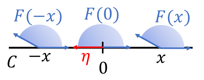
and C:={x∈ℝ2:x2=0}C:=\left\{x\in\mathbb{R}^{2}:x_{2}=0\right\}. Furthermore, consider the function B⁡(x):=−x1B(x):=-x_{1}.

Refer to caption
Figure 1: Illustration of the data of the system ℋf\mathcal{H}_{f} in Example 1.

Note that FF is locally Lipschitz and has closed and convex images. Furthermore, starting from each initial condition xo:=[xo​1xo​2]⊤∈Cx_{o}:=[x_{o1}\quad x_{o2}]^{\top}\in C, the only nontrivial solution is given by ϕ⁡(t):=[xo​1+t0]⊤\phi(t):=[x_{o1}+t\quad 0]^{\top} for all t≥0t\geq 0; hence, C~=C\tilde{C}=C and BB is nonincreasing along each nontrivial solution. However, for xo=0x_{o}=0, we show that, for vo:=[−10]⊤∈F⁡(0)∩TC​(0)v_{o}:=[-1\quad 0]^{\top}\in F(0)\cap T_{C}(0), condition (17) is not satisfied. Indeed, we note that ⟨∇B​(0),vo⟩=1>0\langle\nabla B(0),v_{o}\rangle=1>0. □\square

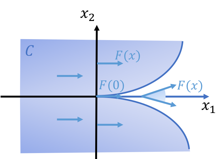
On the other hand, the vectors in F⁡(x)F(x) not generating solutions may affect the global behavior of the solutions in a way that they fail to render the map t↦B⁡(ϕ⁡(t))t\mapsto B(\phi(t)) nonincreasing. The latter is more likely to happen when BB is discontinuous. Consequently, assumptions on some elements of F⁡(x)F(x) not generating solutions should be considered, otherwise, the conditions can fail to be sufficient. In the following example, we propose a constrained system ℋf=(C,F)\mathcal{H}_{f}=(C,F) where FF is locally Lipschitz with closed and convex images, the set CC is closed, and (19) is satisfied. However, the lower semicontinuous function BB fails to be nonincreasing along solutions.

Example 2

Consider the system ℋf=(C,F)\mathcal{H}_{f}=(C,F) with x∈ℝ2x\in\mathbb{R}^{2},

F(x):={[1[−1,1]​x1]⊤if​x1≥0[10]⊤if​x1<0∀x∈C,\displaystyle F(x):=\left\{\begin{matrix}[1\quad[-1,1]x_{1}]^{\top}&\mbox{if}~x_{1}\geq 0\\ [1\quad 0]^{\top}&\mbox{if}~x_{1}<0\end{matrix}\right.\qquad\qquad\forall x\in C,
C:={x∈ℝ2:|x2|≥x12}\displaystyle C:=\left\{x\in\mathbb{R}^{2}:|x_{2}|\geq x_{1}^{2}\right\} ∪{x∈ℝ2:x1≤0}∪{x∈ℝ2:x2=0}.\displaystyle\cup\left\{x\in\mathbb{R}^{2}:x_{1}\leq 0\right\}\cup\left\{x\in\mathbb{R}^{2}:x_{2}=0\right\}.
Refer to caption
Figure 2: Illustration of the data of the system ℋf\mathcal{H}_{f} in Example 2.

Furthermore, consider the lower semicontinuous function

B(x):={0if​x2≤01if​x2>0.B(x):=\left\{\begin{matrix}0&\mbox{if}~x_{2}\leq 0\\ 1&~\mbox{if}~x_{2}>0.\end{matrix}\right.

We will show that in this case condition (19) holds, but the function BB is not nonincreasing along the solutions to ℋf\mathcal{H}_{f}. Indeed, we start noting that

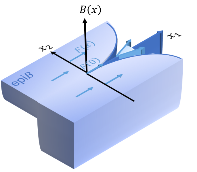
epiB\displaystyle\mathop{\rm epi}B ={(x,r)∈ℝ3:x2≤0,r≥0}∪{(x,r)∈ℝ3:x2>0,r≥1},\displaystyle=\left\{(x,r)\in\mathbb{R}^{3}:x_{2}\leq 0,~r\geq 0\right\}\cup\left\{(x,r)\in\mathbb{R}^{3}:x_{2}>0,~r\geq 1\right\},
epiB∩(C×ℝ)\displaystyle\mathop{\rm epi}B\cap(C\times\mathbb{R}) ={(x,r)∈ℝ3:x2≤0,r≥0,x1≤−x2}∪\displaystyle=\left\{(x,r)\in\mathbb{R}^{3}:x_{2}\leq 0,~r\geq 0,~x_{1}\leq\sqrt{-x_{2}}\right\}\cup
{(x,r)∈ℝ3:x2>0,r≥1,x1≤x2}\displaystyle\left\{(x,r)\in\mathbb{R}^{3}:x_{2}>0,~r\geq 1,~x_{1}\leq\sqrt{x_{2}}\right\}
∪{(x,r)∈ℝ3:x1≥0,r≥0,x2=0}.\displaystyle\cup\left\{(x,r)\in\mathbb{R}^{3}:x_{1}\geq 0,~r\geq 0,~x_{2}=0\right\}.
Refer to caption
Figure 3: Illustration of the set epiB∩(C×ℝ)\mathop{\rm epi}B\cap(C\times\mathbb{R}) in Example 2.

Furthermore, note that FF is locally Lipschitz with closed and convex images. Now, to show that (19) is satisfied, we start noticing that

∂(epiB)∩(C×ℝ)\displaystyle\partial(\mathop{\rm epi}B)\cap(C\times\mathbb{R}) ={(x,r)∈ℝ3:x2<0,r=0,x1≤−x2}\displaystyle=\left\{(x,r)\in\mathbb{R}^{3}:x_{2}<0,~r=0,~x_{1}\leq\sqrt{-x_{2}}\right\}
∪{(x,r)∈ℝ3:x2>0,r=1,x1≤x2}\displaystyle\cup\left\{(x,r)\in\mathbb{R}^{3}:x_{2}>0,~r=1,~x_{1}\leq\sqrt{x_{2}}\right\}
∪{(x,r)∈ℝ3:x2=0,0≤r≤1}.\displaystyle\cup\left\{(x,r)\in\mathbb{R}^{3}:x_{2}=0,~0\leq r\leq 1\right\}.

That is, for each x∈Cx\in C, thus (x,B⁡(x))∈∂(epiB)∩(C×ℝ)(x,B(x))\in\partial(\mathop{\rm epi}B)\cap(C\times\mathbb{R}), we have [F⁡(x)∩TC​(x)0]⊤⊂T∂(epiB)∩(C×ℝ)​(x,B⁡(x))[F(x)\cap T_{C}(x)\quad 0]^{\top}\subset T_{\partial(\mathop{\rm epi}B)\cap(C\times\mathbb{R})}(x,B(x)); hence, (19) follows using [16, Proposition 3.2.3], the fact that

[∂PB⁡(x)−1]⊂NepiB∩(C×ℝ)P​(x,B⁡(x))⊂NepiB∩(C×ℝ)​(x,B⁡(x))∀x∈C,[\partial_{P}B(x)\quad-1]\subset N^{P}_{\mathop{\rm epi}B\cap(C\times\mathbb{R})}(x,B(x))\subset N_{\mathop{\rm epi}B\cap(C\times\mathbb{R})}(x,B(x))\qquad\forall x\in C,

and since C~⊂C\tilde{C}\subset C when CC is closed. Finally, in order to show that the function BB is not nonincreasing along solutions, we consider the function (ϕ⁡(t),B⁡(xo)):=[tt20]⊤∈(C×ℝ)(\phi(t),B(x_{o})):=[t\quad t^{2}\quad 0]^{\top}\in(C\times\mathbb{R}) for all t≥0t\geq 0, which is absolutely continuous and solution to the differential equation (x˙,r˙)=([1x1]⊤,0)∈(F⁡(x),0)(\dot{x},\dot{r})=([1\quad x_{1}]^{\top},0)\in(F(x),0). □\square

To manage such a compromise, extra assumptions on the data (C,F)(C,F) of the system ℋf\mathcal{H}_{f} need to be made.

5 Main Results

In this section, we formulate necessary and sufficient infinitesimal conditions solving Problem 1 when the set CC in ℋf\mathcal{H}_{f} given in (1) is not necessarily ℝn\mathbb{R}^{n}, not necessarily open, and nontrivial solutions are allowed to start from ∂C\partial C.

5.1 When BB is Lower Semicontinuous and C~\tilde{C} is Generic

The proposed approach, in this case, is based on transforming Problem 1 into the characterization of forward pre-invariance of a closed set for an augmented constrained differential inclusion, as described in the following lemma. The proof is in the appendix. Recall that the set C~\tilde{C} is defined in (16).

Lemma 2

Consider a constrained differential inclusion ℋf=(C,F)\mathcal{H}_{f}=(C,F). A lower semicontinuous function B:ℝn→ℝB:\mathbb{R}^{n}\rightarrow\mathbb{R} satisfies ( ⋆ ) ‣ 1 in Problem 1 if and only if the set epiB∩(cl​(C)×ℝ)\mathop{\rm epi}B\cap(\mbox{cl}(C)\times\mathbb{R}) is forward pre-invariant for the extended constrained differential inclusion in (2). □\square

Proof. To prove necessity of epiB∩(cl​(C)×ℝ)\mathop{\rm epi}B\cap(\mbox{cl}(C)\times\mathbb{R}) being forward pre-invariant, we consider a nontrivial solution (ϕ,r):domϕ→ℝn+1(\phi,r):\mathop{\rm dom}\nolimits\phi\rightarrow\mathbb{R}^{n+1} starting from (xo,ro)∈∂(epiB∩(cl​(C)×ℝ))(x_{o},r_{o})\in\partial(\mathop{\rm epi}B\cap(\mbox{cl}(C)\times\mathbb{R})) such that t↦B⁡(ϕ⁡(t))t\mapsto B(\phi(t)) is nonincreasing on domϕ\mathop{\rm dom}\nolimits\phi (note that solutions from int​(epiB∩(cl​(C)×ℝ))\mbox{int}(\mathop{\rm epi}B\cap(\mbox{cl}(C)\times\mathbb{R})) reaching the boundary are already covered by this case). From the definition of the solutions to (1), we conclude that ϕ​(t)∈cl​(C)\phi(t)\in\mbox{cl}(C) for all t∈domϕt\in\mathop{\rm dom}\nolimits\phi. So, to complete the proof of the necessary part, it is enough to show that (ϕ⁡(t),r⁡(t))∈epiB(\phi(t),r(t))\in\mathop{\rm epi}B for all t∈domϕt\in\mathop{\rm dom}\nolimits\phi. Indeed, (xo,ro)∈∂(epiB∩(cl​(C)×ℝ))(x_{o},r_{o})\in\partial(\mathop{\rm epi}B\cap(\mbox{cl}(C)\times\mathbb{R})) implies that either (xo,ro)∈(int​(epiB)∩(cl​(C)×ℝ))(x_{o},r_{o})\in(\mbox{int}(\mathop{\rm epi}B)\cap(\mbox{cl}(C)\times\mathbb{R})), thus ro>B⁡(xo)r_{o}>B(x_{o}), or (xo,ro)∈(∂(epiB)∩(cl​(C)×ℝ))(x_{o},r_{o})\in(\partial(\mathop{\rm epi}B)\cap(\mbox{cl}(C)\times\mathbb{R})), thus ro=B⁡(xo)r_{o}=B(x_{o}). Hence, in both cases ro≥B⁡(xo)r_{o}\geq B(x_{o}). Moreover, since t↦B⁡(ϕ⁡(t))t\mapsto B(\phi(t)) is nonincreasing, it follows that ro≥B⁡(ϕ⁡(t))r_{o}\geq B(\phi(t)) for all t∈domϕt\in\mathop{\rm dom}\nolimits\phi since ϕ⁡(0)=xo∈∂C\phi(0)=x_{o}\in\partial C. The latter fact implies that the solution (ϕ,r)(\phi,r) satisfies (ϕ⁡(t),r⁡(t))∈epiB(\phi(t),r(t))\in\mathop{\rm epi}B for all t∈domϕt\in\mathop{\rm dom}\nolimits\phi and necessity follows.

To prove the sufficient part, we use a contradiction argument. Suppose there exists xo∈cl​(C)x_{o}\in\mbox{cl}(C) and a nontrivial solution ϕ\phi to ℋf\mathcal{H}_{f} such that, for some ϵ>0\epsilon>0, B⁡(ϕ⁡(t))>B⁡(ϕ⁡(0))B(\phi(t))>B(\phi(0)) for all t∈(0,ϵ]t\in(0,\epsilon]. Since the set epiB∩(cl​(C)×ℝ)\mathop{\rm epi}B\cap(\mbox{cl}(C)\times\mathbb{R}) is forward pre-invariant, every solution (ϕ,r)(\phi,r) starting from (xo,B⁡(xo))∈∂(epiB)∩(cl​(C)×ℝ)(x_{o},B(x_{o}))\in\partial(\mathop{\rm epi}B)\cap(\mbox{cl}(C)\times\mathbb{R}) remains in epiB∩(cl​(C)×ℝ)\mathop{\rm epi}B\cap(\mbox{cl}(C)\times\mathbb{R}) for all t∈domϕt\in\mathop{\rm dom}\nolimits\phi. The latter fact implies that (ϕ⁡(t),B⁡(xo))∈epiB(\phi(t),B(x_{o}))\in\mathop{\rm epi}B for all t∈domϕt\in\mathop{\rm dom}\nolimits\phi; hence, B⁡(xo)≥B⁡(ϕ⁡(t))B(x_{o})\geq B(\phi(t)) for all t∈domϕt\in\mathop{\rm dom}\nolimits\phi, which yields a contradiction. ■\blacksquare

Forward pre-invariance has been extensively studied in the literature, see, e.g., [16, 9]. Infinitesimal conditions for forward pre-invariance involving FF and tangent cones with respect to the considered closed set are shown to be necessary and sufficient when C≡ℝnC\equiv\mathbb{R}^{n}. Our approach, in this case, is based on characterizing forward pre-invariance of the set epiB∩(cl​(C)×ℝ)\mathop{\rm epi}B\cap(\mbox{cl}(C)\times\mathbb{R}) using infinitesimal conditions.

Consider the following assumptions on the data (C,F)(C,F) of ℋf\mathcal{H}_{f}:

  1. (M1)

    For each xo∈∂C∩C~x_{o}\in\partial C\cap\tilde{C}, if F⁡(xo)∩TC​(xo)≠∅F(x_{o})\cap T_{C}(x_{o})\neq\emptyset then, for each vo∈F⁡(xo)∩TC​(xo)v_{o}\in F(x_{o})\cap T_{C}(x_{o}), there exist U⁡(xo)U(x_{o}) – a neighborhood of xox_{o} – and a continuous selection v:∂C∩U⁡(xo)→ℝnv:\partial C\cap U(x_{o})\rightarrow\mathbb{R}^{n} such that v⁡(x)∈F⁡(x)∩TC​(x)v(x)\in F(x)\cap T_{C}(x) for all x∈∂C∩U⁡(xo)x\in\partial C\cap U(x_{o}) and v⁡(xo)=vov(x_{o})=v_{o}.

  2. (M2)

    For each xo∈∂C∩C~x_{o}\in\partial C\cap\tilde{C}, there exists U⁡(xo)U(x_{o}) – a neighborhood of xox_{o} – such that F​(x)⊂TC​(x)F(x)\subset T_{C}(x) for all x∈U⁡(xo)∩∂Cx\in U(x_{o})\cap\partial C.

The need for (M1) and (M2) is discussed in Remarks 6 and 10. Furthermore, we consider the following condition:

⟨ζ,v⟩≤0\displaystyle\langle\zeta,v\rangle\leq 0 ∀[ζ⊤​α]⊤∈NepiB∩(C×ℝ)P​(x,B⁡(x)),∀v∈F⁡(x)∩TC​(x),∀x∈C~.\displaystyle\qquad\forall[\zeta^{\top}~\alpha]^{\top}\in N^{P}_{\mathop{\rm epi}B\cap(C\times\mathbb{R})}(x,B(x)),\quad\forall v\in F(x)\cap T_{C}(x),\quad\forall x\in\tilde{C}. (20)

The following result solves Problem 1. Its proof is inspired from [16, Theorem 5.3.4] and [9, Theorem 3.8].

Theorem 1

Consider a system ℋf=(C,F)\mathcal{H}_{f}=(C,F) such that Assumption 1 holds and, additionally, FF is continuous. Let B:ℝn→ℝB:\mathbb{R}^{n}\rightarrow\mathbb{R} be a lower semicontinuous function. Then,

  1. 1.

    ( ⋆ ) ‣ 1 ++ (M1) ⇒\Rightarrow (20).

  2. 2.

    FF locally Lipschitz ++ (20) ++ (M2) ⇒\Rightarrow ( ⋆ ) ‣ 1.

Consequently, when FF is locally Lipschitz and (M1)-(M2) hold, ( ⋆ ) ‣ 1 ⇔\Leftrightarrow (20). □\square

Proof. Using Lemma 2, items 2. and 1. in Theorem 1 follow if the following two statements are proved, respectively.

  1. 1⋆\star.

    The set epiB∩(cl​(C)×ℝ)\mathop{\rm epi}B\cap(\mbox{cl}(C)\times\mathbb{R}) is forward pre-invariant for (2) if (M2) and (20) hold.

  2. 2⋆\star.

    If the set epiB∩(cl​(C)×ℝ)\mathop{\rm epi}B\cap(\mbox{cl}(C)\times\mathbb{R}) is forward pre-invariant for (2) and (M1) holds, then (20) holds.

In order to prove item 2⋆2\star, we assume that the set epiB∩(cl​(C)×ℝ)\mathop{\rm epi}B\cap(\mbox{cl}(C)\times\mathbb{R}) is forward pre-invariant, that is, for each (xo,B⁡(xo))∈∂(epiB)∩(C~×ℝ)(x_{o},B(x_{o}))\in\partial(\mathop{\rm epi}B)\cap(\tilde{C}\times\mathbb{R}), each nontrivial solution starting from (xo,B⁡(xo))(x_{o},B(x_{o})) remains in epiB∩(cl​(C)×ℝ)\mathop{\rm epi}B\cap(\mbox{cl}(C)\times\mathbb{R}) along its entire domain. Furthermore, let us pick vo∈F⁡(xo)∩TC​(xo)v_{o}\in F(x_{o})\cap T_{C}(x_{o}) and using (M1), we conclude the existence of a continuous selection v:∂C∩U⁡(xo)→ℝnv:\partial C\cap U(x_{o})\rightarrow\mathbb{R}^{n} such that v⁡(x)∈F⁡(x)∩TC​(x)v(x)\in F(x)\cap T_{C}(x) for all x∈∂C∩U⁡(xo)x\in\partial C\cap U(x_{o}) and v⁡(xo)=vov(x_{o})=v_{o}. Moreover, since FF is continuous; thus, lower semicontinuous, and has closed and convex images, we use Michael’s selection theorem [18] to conclude that the continuous selection vv on ∂C∩U⁡(xo)\partial C\cap U(x_{o}) can be extended to a continuous selection w:U⁡(xo)→ℝnw:U(x_{o})\rightarrow\mathbb{R}^{n} such that w⁡(x)=v⁡(x)w(x)=v(x) for all x∈∂C∩U⁡(xo)x\in\partial C\cap U(x_{o}). Next, using [16, Proposition 3.4.2], we conclude the existence of a nontrivial solution ϕ\phi starting from xox_{o} solution to the system x˙=w⁡(x)\dot{x}=w(x); thus, ϕ\phi is also solution to ℋf\mathcal{H}_{f} in (1). Next, since the set epiB∩(cl​(C)×ℝ)\mathop{\rm epi}B\cap(\mbox{cl}(C)\times\mathbb{R}) is forward pre-invariant, it follows that t↦(ϕ⁡(t),B⁡(xo))t\mapsto(\phi(t),B(x_{o})) is also a solution to (2) satisfying (ϕ⁡(t),B⁡(xo))⊂epiB∩(cl​(C)×ℝ)(\phi(t),B(x_{o}))\subset\mathop{\rm epi}B\cap(\mbox{cl}(C)\times\mathbb{R}) for all t∈domϕt\in\mathop{\rm dom}\nolimits\phi. Furthermore, consider a sequence {ti}i=0∞→0\left\{t_{i}\right\}^{\infty}_{i=0}\rightarrow 0 and let vi:=ϕ⁡(ti)−ϕ⁡(0)tiv_{i}:=\frac{\phi(t_{i})-\phi(0)}{t_{i}}. Now, since ϕ\phi is solution to x˙=w⁡(x)\dot{x}=w(x) and ww is continuous, it follows that limi→∞vi=vo\lim_{i\rightarrow\infty}v_{i}=v_{o}. At the same time, having (ϕ⁡(ti),B⁡(xo))=((ϕ⁡(0)+vi​ti),B⁡(xo))∈epiB∩(C×ℝ)(\phi(t_{i}),B(x_{o}))=((\phi(0)+v_{i}t_{i}),B(x_{o}))\in\mathop{\rm epi}B\cap(C\times\mathbb{R}) and using the equivalence (see [2, Page 122])

v∈TK​(x)⟺∃{hi}i∈ℕ→0+​and​{vi}i∈ℕ→v:x+hi​vi∈K,\displaystyle v\in T_{K}(x)\Longleftrightarrow\exists\left\{h_{i}\right\}_{i\in\mathbb{N}}\rightarrow 0^{+}~\mbox{and}~\left\{v_{i}\right\}_{i\in\mathbb{N}}\rightarrow v:x+h_{i}v_{i}\in K, (21)

we conclude that [vo⊤0]⊤∈TepiB∩(C×ℝ)​(xo,B⁡(xo))[v_{o}^{\top}\quad 0]^{\top}\in T_{\mathop{\rm epi}B\cap(C\times\mathbb{R})}(x_{o},B(x_{o})). Hence, using44 4 With x=(xo,B⁡(xo))x=(x_{o},B(x_{o})), v=[v⊤0]⊤v=[v^{\top}\quad 0]^{\top}, K=epiB∩(C×ℝ)K=\mathop{\rm epi}B\cap(C\times\mathbb{R}), and NK0=NKN^{0}_{K}=N_{K}. [16, Proposition 3.2.3], we conclude that for each [ζ⊤α]⊤∈NepiB∩(C×ℝ)P​(xo,B⁡(xo))[\zeta^{\top}\quad\alpha]^{\top}\in N^{P}_{\mathop{\rm epi}B\cap(C\times\mathbb{R})}(x_{o},B(x_{o})), [ζ⊤α]⊤∈NepiB∩(C×ℝ)​(xo,B⁡(xo))[\zeta^{\top}\quad\alpha]^{\top}\in N_{\mathop{\rm epi}B\cap(C\times\mathbb{R})}(x_{o},B(x_{o})). Thus, (20) by definition of the normal cone NepiB∩(C×ℝ)N_{\mathop{\rm epi}B\cap(C\times\mathbb{R})}.

Next, we prove item 1⋆1\star using contradiction. Indeed, we consider t1>0t_{1}>0 such that a solution zz to (2) starting from za​o:=(xo,B⁡(xo))∈∂(epiB)∩(C~×ℝ)z_{ao}:=(x_{o},B(x_{o}))\in\partial(\mathop{\rm epi}B)\cap(\tilde{C}\times\mathbb{R}) satisfies za​(t):=(x⁡(t),B⁡(xo))∈(cl​(C)×ℝ)\epiBz_{a}(t):=(x(t),B(x_{o}))\in(\mbox{cl}(C)\times\mathbb{R})\backslash\mathop{\rm epi}B for all t∈(0,t1)t\in(0,t_{1}) and such that

z˙a​(t)∈Fa​(za​(t)):=[F​(x⁡(t))⊤0]⊤for a.a.t∈(0,t1).\dot{z}_{a}(t)\in F_{a}(z_{a}(t)):=[F(x(t))^{\top}\quad 0]^{\top}\quad\mbox{for a.a.}\quad t\in(0,t_{1}).

Furthermore, for t∈[0,t1)t\in[0,t_{1}), we use y⁡(t)y(t) to denote the projection of za​(t)z_{a}(t) on the set epiB∩(cl​(C)×ℝ)\mathop{\rm epi}B\cap(\mbox{cl}(C)\times\mathbb{R}) and we define

δ⁡(t):=|za​(t)−y⁡(t)|∀t∈[0,t1).\delta(t):=|z_{a}(t)-y(t)|\qquad\forall t\in[0,t_{1}).

That is, by construction, we have δ⁡(0)=0\delta(0)=0 and δ⁡(t)>0\delta(t)>0 for all t∈(0,t1)t\in(0,t_{1}) for t1t_{1} sufficiently small. Now, using the fact that

δ⁡(t+h)=|za​(t+h)−y⁡(t+h)|≤|za​(t+h)−y⁡(t)|,\delta(t+h)=|z_{a}(t+h)-y(t+h)|\leq|z_{a}(t+h)-y(t)|,

plus the identity a−b=(a2−b2)/(a+b)a-b=(a^{2}-b^{2})/(a+b) for aa and b≥0b\geq 0, we derive the following inequality for some h>0h>0 sufficiently small

δ⁡(t+h)−δ⁡(t)\displaystyle\delta(t+h)-\delta(t) ≤|za​(t+h)−y⁡(t)|−|za​(t)−y⁡(t)|\displaystyle\leq|z_{a}(t+h)-y(t)|-|z_{a}(t)-y(t)| (22)
=|za​(t+h)−y⁡(t)|2−|za​(t)−y⁡(t)|2|za​(t+h)−y⁡(t)|+|za​(t)−y⁡(t)|.\displaystyle=\frac{|z_{a}(t+h)-y(t)|^{2}-|z_{a}(t)-y(t)|^{2}}{|z_{a}(t+h)-y(t)|+|z_{a}(t)-y(t)|}.

Furthermore, assume that tt is chosen such that z˙a​(t)\dot{z}_{a}(t) exists. Hence, we can replace za​(t+h)z_{a}(t+h) by

za​(t+h)=za​(t)+h​z˙a​(t)+o⁡(h),\displaystyle z_{a}(t+h)=z_{a}(t)+h\dot{z}_{a}(t)+o(h), (23)

where o⁡(h)o(h) is the remainder of the first order Taylor expansion of h↦za​(t+h)h\mapsto z_{a}(t+h) around h=0h=0, which satisfies limh→0o⁡(h)/h=0\lim_{h\rightarrow 0}o(h)/h=0. Furthermore, using the inequality

|za​(t+h)−y⁡(t)|≥|za​(t)−y⁡(t)|−h​|z˙a​(t)+o⁡(h)/h|,|z_{a}(t+h)-y(t)|\geq|z_{a}(t)-y(t)|-h|\dot{z}_{a}(t)+o(h)/h|,

we conclude that the denominator in (22) satisfies

|za​(t+h)−y⁡(t)|+\displaystyle|z_{a}(t+h)-y(t)|+ |za​(t)−y⁡(t)|≥2​|za​(t)−y⁡(t)|−h​|z˙a​(t)+o⁡(h)/h|\displaystyle|z_{a}(t)-y(t)|\geq 2|z_{a}(t)-y(t)|-h|\dot{z}_{a}(t)+o(h)/h|

while the numerator in (22) is upper bounded by

2​z˙a​(t)⊤\displaystyle 2\dot{z}_{a}(t)^{\top} (za​(t)−y⁡(t))+h2​|z˙a​(t)+o⁡(h)/h|2+2​o​(h)⊤​(za​(t)−y⁡(t)).\displaystyle(z_{a}(t)-y(t))+h^{2}|\dot{z}_{a}(t)+o(h)/h|^{2}+2o(h)^{\top}(z_{a}(t)-y(t)).

Hence, letting h→0+h\rightarrow 0^{+} we obtain,

lim suph→0+δ⁡(t+h)−δ⁡(t)h≤(za​(t)−y⁡(t))⊤​z˙a​(t)|za​(t)−y​(t)|.\displaystyle\limsup_{h\rightarrow 0^{+}}\frac{\delta(t+h)-\delta(t)}{h}\leq\frac{(z_{a}(t)-y(t))^{\top}\dot{z}_{a}(t)}{|z_{a}(t)-y(t)|}. (24)

We have the following claim.

Claim 1

Under (20), (M2), and when t>0t>0 is sufficiently small, the following holds:

(za​(t)−y⁡(t))⊤​ηy≤0∀ηy∈Fa​(y⁡(t)).\displaystyle(z_{a}(t)-y(t))^{\top}\eta_{y}\leq 0\qquad\forall\eta_{y}\in F_{a}(y(t)). (25)

∙\bullet

Under (25) and for each ηy∈Fa​(y⁡(t))\eta_{y}\in F_{a}(y(t)), the inequality (24) can be re-written as

lim suph→0+δ⁡(t+h)−δ⁡(t)h≤\displaystyle\limsup_{h\rightarrow 0^{+}}\frac{\delta(t+h)-\delta(t)}{h}\leq (za​(t)−y⁡(t))⊤​[z˙a​(t)−ηy]|za​(t)−y​(t)|.\displaystyle\frac{(z_{a}(t)-y(t))^{\top}[\dot{z}_{a}(t)-\eta_{y}]}{|z_{a}(t)-y(t)|}. (26)

Since z˙a​(t)∈Fa​(za​(t))\dot{z}_{a}(t)\in F_{a}(z_{a}(t)), using the fact that the map FaF_{a} is locally Lipschitz, it is always possible to find a constant γ>0\gamma>0 and ηy∗∈F⁡(y⁡(t))\eta^{*}_{y}\in F(y(t)) such that, when replacing ηy\eta_{y} by ηy∗\eta_{y}^{*} in (26), we obtain, for almost all t∈(0,t1)t\in(0,t_{1}),

lim suph→0+δ⁡(t+h)−δ⁡(t)h≤\displaystyle\limsup_{h\rightarrow 0^{+}}\frac{\delta(t+h)-\delta(t)}{h}\leq γ​|za​(t)−y|=γ​δ​(t).\displaystyle\gamma|z_{a}(t)-y|=\gamma\delta(t). (27)

The contradiction follows since (27) implies that δ⁡(t)=0\delta(t)=0 for all t∈(0,t1)t\in(0,t_{1}) due to δ⁡(0)=0\delta(0)=0 by construction.

Proof of Claim 1: To prove the latter claim, we start noticing, using the continuity of the system’s solutions, that for any neighborhood sufficiently small around za​oz_{ao} denoted U⁡(za​o)U(z_{ao}), there exists t1>0t_{1}>0 sufficiently small such that y⁡(t)∈U⁡(za​o)y(t)\in U(z_{ao}) for all t∈[0,t1)t\in[0,t_{1}). Furthermore, under (M2) and for U⁡(za​o)U(z_{ao}) small enough, we show that y⁡(t)y(t) either belongs to ∂(epiB)∩(C~×ℝ)\partial(\mathop{\rm epi}B)\cap(\tilde{C}\times\mathbb{R}) or to the set int​(epiB)∩(∂C×ℝ)\mbox{int}(\mathop{\rm epi}B)\cap(\partial C\times\mathbb{R}). Indeed, by definition of the projection, y⁡(t)y(t) cannot belong to int​(epiB)∩(int​(C)×ℝ)=int​(epiB∩(C×ℝ))\mbox{int}(\mathop{\rm epi}B)\cap(\mbox{int}(C)\times\mathbb{R})=\mbox{int}(\mathop{\rm epi}B\cap(C\times\mathbb{R})). Furthermore, (M2) implies that, when U⁡(za​o)U(z_{ao}) is small enough, a nontrivial solution starting from y⁡(t)y(t) always exists; hence, y⁡(t)∈C~×ℝy(t)\in\tilde{C}\times\mathbb{R}. Now, we consider the two possibilities of y⁡(t)y(t).

  • •

    When y⁡(t)∈∂(epiB)∩(C~×ℝ)y(t)\in\partial(\mathop{\rm epi}B)\cap(\tilde{C}\times\mathbb{R}), (25) follows from (20). Indeed, by definition of NepiB∩(C×ℝ)PN^{P}_{\mathop{\rm epi}B\cap(C\times\mathbb{R})}, we conclude that za​(t)−y⁡(t)∈NepiB∩(C×ℝ)P​(y⁡(t))z_{a}(t)-y(t)\in N^{P}_{\mathop{\rm epi}B\cap(C\times\mathbb{R})}(y(t)). Furthermore, using (M2) for t>0t>0 small enough, we conclude that Fa​(y⁡(t))⊂TepiB∩(C×ℝ)​(y⁡(t))F_{a}(y(t))\subset T_{\mathop{\rm epi}B\cap(C\times\mathbb{R})}(y(t)).

  • •

    When y⁡(t)∈int​(epiB)∩(∂C×ℝ)y(t)\in\mbox{int}(\mathop{\rm epi}B)\cap(\partial C\times\mathbb{R}), since y⁡(t)∈U⁡(za​o)y(t)\in U(z_{ao}), it follows using (M2) that Fa​(y⁡(t))⊂TC​(y⁡(t))F_{a}(y(t))\subset T_{C}(y(t)). Furthermore, since y​(t)∈int​(epiB)y(t)\in\mbox{int}(\mathop{\rm epi}B), it follows that Fa​(y⁡(t))⊂TepiB∩(C×ℝ)​(y⁡(t))F_{a}(y(t))\subset T_{\mathop{\rm epi}B\cap(C\times\mathbb{R})}(y(t)).

Now, in order to conclude (25), for each ηy∈Fa​(y⁡(t))\eta_{y}\in F_{a}(y(t)), we introduce the inequality, for some h>0h>0,

|za​(t)−y⁡(t)|≤|za​(t)−y⁡(t)−h​ηy|+|y⁡(t)+h​ηy|K,\displaystyle|z_{a}(t)-y(t)|\leq|z_{a}(t)-y(t)-h\eta_{y}|+|y(t)+h\eta_{y}|_{K}, (28)

where K:=epiB∩(C×ℝ)K:=\mathop{\rm epi}B\cap(C\times\mathbb{R}). To obtain the previous inequality, we used the fact that |⋅|K|\cdot|_{K} is globally Lipschitz with Lipschitz constant equal to 11 and |za​(t)−y⁡(t)|=|za​(t)|K|z_{a}(t)-y(t)|=|z_{a}(t)|_{K}. Next, by taking the square in both sides of inequality (28) and dividing by hh, we obtain, for each ηy∈Fa​(y⁡(t))\eta_{y}\in F_{a}(y(t)),

|za​(t)−y⁡(t)|2h≤|za​(t)−y⁡(t)−h​ηy|2h+|y⁡(t)+h​ηy|K2h\displaystyle\frac{|z_{a}(t)-y(t)|^{2}}{h}\leq\frac{|z_{a}(t)-y(t)-h\eta_{y}|^{2}}{h}+\frac{|y(t)+h\eta_{y}|_{K}^{2}}{h}
+2​|za​(t)−y⁡(t)−h​ηy|​|y⁡(t)+h​ηy|Kh\displaystyle+\frac{2|z_{a}(t)-y(t)-h\eta_{y}||y(t)+h\eta_{y}|_{K}}{h}
≤\displaystyle\leq |za​(t)−y⁡(t)|2h+h​|ηy|2−2​(za​(t)−y⁡(t))​ηy+h​(|y⁡(t)+h​ηy|Kh)2\displaystyle\frac{|z_{a}(t)-y(t)|^{2}}{h}+h|\eta_{y}|^{2}-2(z_{a}(t)-y(t))\eta_{y}+h\left(\frac{|y(t)+h\eta_{y}|_{K}}{h}\right)^{2}
+2​|za​(t)−y⁡(t)−h​ηy|​|y⁡(t)+h​ηy|Kh.\displaystyle+\frac{2|z_{a}(t)-y(t)-h\eta_{y}||y(t)+h\eta_{y}|_{K}}{h}.

Finally, letting h→0+h\rightarrow 0^{+} through a suitable sequence, (25) is proven using the fact that lim infh→0+|y⁡(t)+h​ηy|Kh=0\liminf_{h\rightarrow 0^{+}}\frac{|y(t)+h\eta_{y}|_{K}}{h}=0 since we already have ηy∈TK​(y⁡(t))\eta_{y}\in T_{K}(y(t)). ■\blacksquare

Remark 6

Condition (M1) ensures the existence of a nontrivial solution (i.e., solution whose domain is not a singleton) along each direction in the intersection between the images of FF and the contingent cone TCT_{C}. The latter requirement is necessary in order to prove the necessary part of the statement in the general case where CC is not ℝn\mathbb{R}^{n} and nontrivial solutions start from ∂C\partial C, see Example 1.

In other words, when t↦B⁡(ϕ⁡(t))t\mapsto B(\phi(t)) is nonincreasing along the nontrivial solutions to ℋf\mathcal{H}_{f}, showing that, for each xo∈C~x_{o}\in\tilde{C}, every vo∈F⁡(xo)∩TC​(xo)v_{o}\in F(x_{o})\cap T_{C}(x_{o}) satisfies (20) naturally imposes the existence of at least one nontrivial solution starting from xox_{o} that is tangent to vov_{o} at xox_{o}. ∙\bullet

Remark 7

The existence of a nontrivial solution along each direction within the set F⁡(xo)F(x_{o}) holds for free when xo∈int​(C)x_{o}\in\mbox{int}(C). Indeed, in this case, for each vo∈F⁡(xo)∩TC​(xo)=F⁡(xo)v_{o}\in F(x_{o})\cap T_{C}(x_{o})=F(x_{o}), there exists a selection v:U⁡(xo)→ℝnv:U(x_{o})\rightarrow\mathbb{R}^{n}, U⁡(xo)⊂CU(x_{o})\subset C, such that v⁡(x)∈F⁡(x)v(x)\in F(x) for all x∈U⁡(xo)x\in U(x_{o}) and v⁡(xo)=vov(x_{o})=v_{o}. The latter selection can be chosen to be continuous when FF is locally Lipschitz. Hence, the differential equation x˙=v⁡(x)\dot{x}=v(x) admits a continuously differentiable solution ϕ\phi starting from xox_{o} with ϕ˙​(0)=vo\dot{\phi}(0)=v_{o}, which is also solution to ℋf\mathcal{H}_{f}; thus, the solution ϕ\phi is tangent to vov_{o} at xox_{o}. ∙\bullet

Remark 8

The assumption (M1) holds for free for example if CC is closed, dom(F∩TC)∩∂C\mathop{\rm dom}\nolimits(F\cap T_{C})\cap\partial C is open relative to ∂C\partial C, F∩TCF\cap T_{C} is lower semicontinuous at least on dom(F∩TC)∩∂C\mathop{\rm dom}\nolimits(F\cap T_{C})\cap\partial C, and the set CC is regular. Indeed, having TC​(x)=CC​(x)T_{C}(x)=C_{C}(x) for all x∈cl​(C)x\in\mbox{cl}(C) implies that TCT_{C} is convex for all x∈cl​(C)x\in\mbox{cl}(C) and the same holds for F​(x)∩TC​(x)F(x)\cap T_{C}(x) since F⁡(x)F(x) is also convex for all x∈Cx\in C. Hence, a direct application of Michæl’s Theorem [18, Theorem 3.2] to the set-valued map F∩TCF\cap T_{C} defined on the open set dom(F∩TC)∩∂C\mathop{\rm dom}\nolimits(F\cap T_{C})\cap\partial C relative to ∂C\partial C, (M1) follows. ∙\bullet

Remark 9

Assumption (M1) can be replaced by the following relaxed assumption involving some extra knowledge concerning the system’s solutions.

  1. (M1’)

    For each xo∈∂C∩C~x_{o}\in\partial C\cap\widetilde{C} and for each vo∈F⁡(xo)∩TC​(xo)v_{o}\in F(x_{o})\cap T_{C}(x_{o}), there exists a solution ϕ:[0,h]↦ϕ⁡(t)\phi:[0,h]\mapsto\phi(t), for some h>0h>0, starting from xox_{o} and a sequence {hi}i=0∞→0\left\{h_{i}\right\}^{\infty}_{i=0}\rightarrow 0 and limi→∞(ϕ⁡(hi)−xo)/hi=vo\lim_{i\rightarrow\infty}(\phi(h_{i})-x_{o})/h_{i}=v_{o}.

∙\bullet

Remark 10

When (M2) is not satisfied, as shown in Example 2, there exist situations where the statement of Theorem 1 does not hold even if all the remaining conditions therein are satisfied. As a consequence, constraining more vector fields rather than only those in F​(x)∩TC​(x)F(x)\cap T_{C}(x), as proposed in (20), is important to prove the sufficient part in Theorem 1. However, strengthening (20) would affect the statement in 2., the reason why a global assumption similar to (M2) that is independent from the function BB must be considered. ∙\bullet

In the following, we show how Theorem 1 applies to solve Problem 1 on a concrete example.

Example 3

The continuous dynamics of the bouncing-ball hybrid model is given by ℋf:=(C,F)\mathcal{H}_{f}:=(C,F) with F⁡(x):=[x2−γ]⊤F(x):=[x_{2}\quad-\gamma]^{\top} for all x∈C:={x∈ℝ2:x1≥0}x\in C:=\left\{x\in\mathbb{R}^{2}:x_{1}\geq 0\right\}. The constant γ>0\gamma>0 is the gravitational acceleration. First, FF is single valued and continuously differentiable; hence, Assumption 1 holds. Second, note that C~:=C\{x∈ℝ2:x1=0,x2≤0}\widetilde{C}:=C\backslash\left\{x\in\mathbb{R}^{2}:x_{1}=0,~x_{2}\leq 0\right\}. Hence, starting from xo∈C~∩∂C={x∈ℝ2:x1=0,x2>0}x_{o}\in\widetilde{C}\cap\partial C=\left\{x\in\mathbb{R}^{2}:x_{1}=0,\quad x_{2}>0\right\}, F⁡(xo)=[xo​2−γ]⊤∈TC​(xo)F(x_{o})=[x_{o2}\quad-\gamma]^{\top}\in T_{C}(x_{o}); thus, (M2) follows. Moreover, (M1) is also satisfied since ∂C∩C~\partial C\cap\widetilde{C} is open and, for each xo∈∂C∩C~x_{o}\in\partial C\cap\widetilde{C}, F⁡(xo)∈TC​(xo)F(x_{o})\in T_{C}(x_{o}). Finally, using Theorem 1, we conclude that a lower semicontinuous function B:ℝ2→ℝB:\mathbb{R}^{2}\rightarrow\mathbb{R} satisfies ( ⋆ ) ‣ 1 if and only if (20) holds. In particular, the energy function of the bouncing ball satisfies (20) since, by definition, it cannot increase along the solutions. □\square

The following result shows that, in some situations, (M1) is not needed. However, such situations require that the set C~\widetilde{C} and the function BB satisfy the following extra assumptions:

Assumption 2

x↦blckdiag​{In,0}​NepiB∩(C×ℝ)P​(x,B⁡(x))x\mapsto\mbox{blckdiag}\left\{I_{n},0\right\}N^{P}_{\mathop{\rm epi}B\cap(C\times\mathbb{R})}(x,B(x)) is lower semicontinuous on C~\widetilde{C}. ∙\bullet

Assumption 3

U​(x)∩int​(C)≠∅U(x)\cap\mbox{int}(C)\neq\emptyset for all x∈∂C∩Cx\in\partial C\cap C and for all U⁡(x)U(x). ∙\bullet

Theorem 2

Consider a system ℋf=(C,F)\mathcal{H}_{f}=(C,F) such that Assumption 1 holds and FF is additionally continuous. Let B:ℝn→ℝB:\mathbb{R}^{n}\rightarrow\mathbb{R} be a lower semicontinuous function. Then,

Consequently, when FF is locally Lipschitz and (M2) and Assumptions 2-3 hold, ( ⋆ ) ‣ 1 ⇔\Leftrightarrow (20). □\square

Proof. We distinguish two situations.

  • •

    First, we consider the case where x∈int​(C)x\in\mbox{int}(C). In this case, according to Remark 7, (M1) holds trivially. Hence, using Theorem 1, we conclude that

    ⟨ζ,v⟩≤0\displaystyle\langle\zeta,v\rangle\leq 0 ∀[ζ⊤​α]⊤∈NepiB∩(C×ℝ)P​(x,B⁡(x)),∀v∈F⁡(x)∩TC​(x).\displaystyle\qquad\forall[\zeta^{\top}~\alpha]^{\top}\in N^{P}_{\mathop{\rm epi}B\cap(C\times\mathbb{R})}(x,B(x)),\quad\forall v\in F(x)\cap T_{C}(x). (29)
  • •

    Next, when x∈C~\int​(C)x\in\widetilde{C}\backslash\mbox{int}(C), we show that (29) holds using a contradiction. That is, let us assume the existence of [ζo⊤αo]⊤∈NepiB∩(C×ℝ)P​(x,B⁡(x))[\zeta_{o}^{\top}\quad\alpha_{o}]^{\top}\in N^{P}_{\mathop{\rm epi}B\cap(C\times\mathbb{R})}(x,B(x)) and vo∈F⁡(x)∩TC​(x)v_{o}\in F(x)\cap T_{C}(x) such that ⟨ζo,vo⟩>0\langle\zeta_{o},v_{o}\rangle>0; thus, ⟨ζo,vo⟩≥ϵ\langle\zeta_{o},v_{o}\rangle\geq\epsilon for some ϵ>0\epsilon>0. Next, using the continuity of FF both with Assumption 3, we conclude that for each ϵ1>0\epsilon_{1}>0 there exist U⁡(x)U(x) such that for each y∈U​(x)∩int​(C)y\in U(x)\cap\mbox{int}(C) (U​(x)∩int​(C)≠∅U(x)\cap\mbox{int}(C)\neq\emptyset under Assumption 3) there exists vy∈F⁡(y)v_{y}\in F(y) such that |vy−vo|≤ϵ1|v_{y}-v_{o}|\leq\epsilon_{1}. On the other hand, using Assumption 2 under Assumption 3, we conclude the existence of x1∈U⁡(x)∩int​(C)x_{1}\in U(x)\cap\mbox{int}(C) sufficiently close to xx and [ζ1α1]⊤∈NepiB∩(C×ℝ)P​(x1,B⁡(x1))[\zeta_{1}\quad\alpha_{1}]^{\top}\in N^{P}_{\mathop{\rm epi}B\cap(C\times\mathbb{R})}(x_{1},B(x_{1})) such that |ζ1−ζo|≤ϵ1|\zeta_{1}-\zeta_{o}|\leq\epsilon_{1}. Furthermore, since x1∈int​(C)x_{1}\in\mbox{int}(C), using the first part of the proof, we conclude that ⟨ζ1,vx1⟩≤0\langle\zeta_{1},v_{x_{1}}\rangle\leq 0. However, since ⟨ζo,vo⟩≥ϵ\langle\zeta_{o},v_{o}\rangle\geq\epsilon it follows that

    ⟨ζo,vo⟩\displaystyle\langle\zeta_{o},v_{o}\rangle =⟨ζ1,vx1⟩+⟨(ζo−ζ1),vo⟩+⟨ζo,(vo−vx1)⟩\displaystyle=\langle\zeta_{1},v_{x_{1}}\rangle+\langle(\zeta_{o}-\zeta_{1}),v_{o}\rangle+\langle\zeta_{o},(v_{o}-v_{x_{1}})\rangle
    +⟨(ζ1−ζo),(vo−vx1)⟩\displaystyle+\langle(\zeta_{1}-\zeta_{o}),(v_{o}-v_{x_{1}})\rangle
    ≥ϵ.\displaystyle\geq\epsilon.

    Hence, ⟨ζ1,vx1⟩≥ϵ−(|vo|+|ζo|)​ϵ1−ϵ12\langle\zeta_{1},v_{x_{1}}\rangle\geq\epsilon-(|v_{o}|+|\zeta_{o}|)\epsilon_{1}-\epsilon_{1}^{2}. Finally, taking

    ϵ1=min⁡{ϵ2​((|vo|+|ζo|)+1),1},\epsilon_{1}=\min\left\{\frac{\epsilon}{2((|v_{o}|+|\zeta_{o}|)+1)},1\right\},

    the contradiction follows since the latter implies that ⟨ζ1,vx1⟩≥ϵ/2>0\langle\zeta_{1},v_{x_{1}}\rangle\geq\epsilon/2>0.

■\blacksquare

In the sequel, we will show that the inequality in (20) does not need to be checked for all [ζ⊤α]⊤∈NepiB∩(C×ℝ)P​(x,B⁡(x))[\zeta^{\top}\quad\alpha]^{\top}\in N^{P}_{\mathop{\rm epi}B\cap(C\times\mathbb{R})}(x,B(x)) when x∈int​(C)x\in\mbox{int}(C). That is, when x∈int​(C)x\in\mbox{int}(C), we will show that it is enough to verify the inequality in (20) only for the vectors [ζ⊤​α]⊤∈NepiB∩(cl​(C)×ℝ)P​(x,B⁡(x))[\zeta^{\top}~\alpha]^{\top}\in N^{P}_{\mathop{\rm epi}B\cap(\mbox{cl}(C)\times\mathbb{R})}(x,B(x)) with α=−1\alpha=-1 to conclude that it holds for all [ζ⊤α]⊤∈NepiB∩(C×ℝ)P​(x,B⁡(x))[\zeta^{\top}\quad\alpha]^{\top}\in N^{P}_{\mathop{\rm epi}B\cap(C\times\mathbb{R})}(x,B(x)). The former subset is generated by the proximal subdifferential ∂PB\partial_{P}B introduced in (15). Although ∂PB\partial_{P}B can fail to exist at some points (x,B⁡(x))∈epiB∩(int​(C)×ℝ)(x,B(x))\in\mathop{\rm epi}B\cap(\mbox{int}(C)\times\mathbb{R}), its density property in Lemma 3 in the Appendix is enough to preserve the equivalence in Theorem 1.

Proposition 1

Consider a system ℋf=(C,F)\mathcal{H}_{f}=(C,F) such that Assumption 1 holds, FF is additionally locally Lipschitz, and let B:ℝn→ℝB:\mathbb{R}^{n}\rightarrow\mathbb{R} be a lower semicontinuous function. Then, (29) is satisfied at x∈int​(C)x\in\mbox{int}(C) if

⟨ζ,η⟩≤0∀ζ∈∂PB⁡(x),∀η∈F⁡(x).\displaystyle\langle\zeta,\eta\rangle\leq 0\qquad\forall\zeta\in\partial_{P}B(x),\qquad\forall\eta\in F(x). (30)

□\square

Proof. Let x∈int​(C)x\in\mbox{int}(C) and let [ζ⊤0]⊤∈NSP​(x,B⁡(x))[\zeta^{\top}\quad 0]^{\top}\in N^{P}_{S}(x,B(x)). After Lemma 3, we conclude the existence of a sequence (xi,ϵi,ζi)∈int​(C)×ℝ>0×∂PB⁡(xi)(x_{i},\epsilon_{i},\zeta_{i})\in\mbox{int}(C)\times\mathbb{R}_{>0}\times\partial_{P}B(x_{i}) such that (xi,ϵi,ζi)→(x,0,ζ)(x_{i},\epsilon_{i},\zeta_{i})\rightarrow(x,0,\zeta) and [ζi⊤−ϵi]⊤∈NepiBP​(xi,B⁡(xi))[\zeta_{i}^{\top}\quad-\epsilon_{i}]^{\top}\in N^{P}_{\mathop{\rm epi}B}(x_{i},B(x_{i})). Moreover, since FF is locally Lipschitz, it follows that, for each ηx∈F⁡(x)\eta_{x}\in F(x), there exists vi∈F⁡(xi)v_{i}\in F(x_{i}) such that |vi−ηx|≤K​|xi−x||v_{i}-\eta_{x}|\leq K|x_{i}-x| for some K>0K>0. According to (30), we conclude that, for all i∈ℕi\in\mathbb{N},

⟨ζi,vi⟩=⟨ζ,ηx⟩+⟨ζi,vi−ηx⟩+⟨ζi−ζ,ηx⟩≤0.\displaystyle\langle\zeta_{i},v_{i}\rangle=\langle\zeta,\eta_{x}\rangle+\langle\zeta_{i},v_{i}-\eta_{x}\rangle+\langle\zeta_{i}-\zeta,\eta_{x}\rangle\leq 0.

Finally, on the limit we conclude that ⟨ζ,ηx⟩≤0\langle\zeta,\eta_{x}\rangle\leq 0 for all ηx∈F⁡(x)\eta_{x}\in F(x). ■\blacksquare

5.2 When BB is Lower Semicontinuous and cl(C)\mathop{\rm cl}\nolimits(C) is Pre-Contractive

When the set C≡ℝnC\equiv\mathbb{R}^{n}, or when C~\widetilde{C} is open, the following necessary and sufficient infinitesimal condition solving Problem 1 is provided in [9, Theorem 6.3].

⟨ζ,η⟩≤0∀ζ∈∂PB⁡(x),∀η∈F⁡(x),∀x∈int​(C).\displaystyle\langle\zeta,\eta\rangle\leq 0\qquad\forall\zeta\in\partial_{P}B(x),\qquad\forall\eta\in F(x),\qquad\forall x\in\mbox{int}(C). (31)

In the following statement, we recover [9, Theorem 6.3] as a direct consequence of Theorem 1 and Proposition 1. Furthermore, as we will show, Condition (31) can also be used when the following extra assumptions hold.

Assumption 4

The set cl(C)\mathop{\rm cl}\nolimits(C) is pre-contractive. ∙\bullet

Assumption 5

BB is continuous on ∂C∩C~\partial C\cap\widetilde{C}. ∙\bullet

Corollary 1

Consider a system ℋf=(C,F)\mathcal{H}_{f}=(C,F) such that Assumption 1 holds and FF is additionally continuous. Let B:ℝn→ℝB:\mathbb{R}^{n}\rightarrow\mathbb{R} be a lower semicontinuous function. Then,

  1. 1.

    ( ⋆ ) ‣ 1 ⇒\Rightarrow (31).

  2. 2.

    When FF is locally Lipschitz and either C~\widetilde{C} is open or Assumptions 4-5 hold, ( ⋆ ) ‣ 1 ⇔\Leftrightarrow (31).

□\square

Proof. The proof of item 11 follows from the first item in Theorem 1 since (M1) holds trivially when xo∈int​(C)x_{o}\in\mbox{int}(C), see Remark 7.

The proof of item 22, when C~\widetilde{C} is open, follows from a direct application of Theorem 1 and Proposition 1. Indeed, we notice that when C~\widetilde{C} is open, (M1) and (M2) hold trivially because ∂C∩C~=∅\partial C\cap\widetilde{C}=\emptyset. Now, we assume that Assumptions 4-5 hold. Using the previous step, we conclude that, along the solutions ϕ:domϕ→int​(C)\phi:\mathop{\rm dom}\nolimits\phi\rightarrow\mbox{int}(C), t↦B⁡(ϕ⁡(t))t\mapsto B(\phi(t)) is nonincreasing if and only if (30) holds. To complete the proof, we will show that, under Assumptions 4-5, if t↦B⁡(ϕ⁡(t))t\mapsto B(\phi(t)) is nonincreasing along the solutions ϕ:domϕ→int​(C)\phi:\mathop{\rm dom}\nolimits\phi\rightarrow\mbox{int}(C) then so it is along the solutions ϕ:domϕ→cl​(C)\phi:\mathop{\rm dom}\nolimits\phi\rightarrow\mbox{cl}(C) using contradiction. Consider a solution ϕ:domϕ→cl​(C)\phi:\mathop{\rm dom}\nolimits\phi\rightarrow\mbox{cl}(C) such that t↦B⁡(ϕ⁡(t))t\mapsto B(\phi(t)) fails to be nonincreasing. Since ϕ\phi cannot flow in ∂C\partial C under Assumption 4, t↦B⁡(ϕ⁡(t))t\mapsto B(\phi(t)) is nonincreasing in the interior CC, and since BB is only lower semicontinuous, for the map t↦B⁡(ϕ⁡(t))t\mapsto B(\phi(t)) to fail to be nonincreasing either one of the following holds: For some ϵ>0\epsilon>0, B⁡(ϕ⁡(0))<B⁡(ϕ⁡(t))B(\phi(0))<B(\phi(t)) for all t∈(0,ϵ]t\in(0,\epsilon], or, for some T>0T>0 such that ϕ⁡(T)∈∂C\phi(T)\in\partial C, B⁡(ϕ⁡(T))>B⁡(ϕ⁡(T−t))B(\phi(T))>B(\phi(T-t)) for all t∈(0,ϵ]t\in(0,\epsilon]. The latter scenario contradicts the lower semicontinuity of BB, and the first one contradicts Assumption 5. ■\blacksquare

Before closing this section, the following remark is in order.

Remark 11

It is important to notice that, when x∈∂C∩C~x\in\partial C\cap\widetilde{C}, we need to impose a condition similar to (20) since the relaxed condition in (30) is not enough to guarantee the equivalence. Indeed, when x∈int​(C)x\in\mbox{int}(C), (30) indicates that the inequality therein holds for all [ζ−1]⊤∈NepiB∩(C×ℝ)P​(x,B⁡(x))[\zeta\quad-1]^{\top}\in N^{P}_{\mathop{\rm epi}B\cap(C\times\mathbb{R})}(x,B(x)), moreover, when [ζ0]⊤∈NepiB∩(C×ℝ)P​(x,B⁡(x))[\zeta\quad 0]^{\top}\in N^{P}_{\mathop{\rm epi}B\cap(C\times\mathbb{R})}(x,B(x)), it is possible to show that the inequality in (30) remains satisfied using Lemma 3. Hence, using Lemma 3, we can find a point in any neighborhood of U⁡(x)U(x) such that (30) holds. The latter fact is not necessarily true when x∈∂C∩C~x\in\partial C\cap\widetilde{C}, since the points in the neighborhood of xx are not necessarily in C~\widetilde{C}; thus, there is no guarantee to find a point within any neighborhood of xx such that (30) holds. ∙\bullet

5.3 When BB is Locally Lipschitz and C~\tilde{C} is Generic

In this case, we show that (M2) is not required. Indeed, such a relaxation is possible since the generalized gradient ∂CB\partial_{C}B introduced in Definition 4 will be used instead of the proximal subdifferential. Thanks to Lebourg’s mean-value Theorem in Lemma 4 and to the lower Dini-derivative-based condition in Lemma 1, which combined together provide a useful relation between the lower Dini derivative of BB along the system’s solutions and the generalized gradient ∂CB\partial_{C}B.

In this section, we consider the following infinitesimal conditions:

⟨η,ζ⟩\displaystyle\langle\eta,\zeta\rangle ≤0∀η∈∂CB⁡(x),∀ζ∈F⁡(x)∩TC​(x),∀x∈C~.\displaystyle\leq 0\quad\forall\eta\in\partial_{C}B(x),\quad\forall\zeta\in F(x)\cap T_{C}(x),\quad\forall x\in\widetilde{C}. (32)
⟨η,ζ⟩\displaystyle\langle\eta,\zeta\rangle ≤0∀η∈∂CB⁡(x),∀ζ∈F⁡(x)∩TC​(x):∃c∈ℝ:⟨η,ζ⟩=c​∀η∈∂CB⁡(x),\displaystyle\leq 0\quad\forall\eta\in\partial_{C}B(x),\quad\forall\zeta\in F(x)\cap T_{C}(x):\exists c\in\mathbb{R}:\langle\eta,\zeta\rangle=c~\forall\eta\in\partial_{C}B(x),
∀x∈C~.\displaystyle\qquad\qquad\forall x\in\widetilde{C}. (33)

Furthermore, we recall from [29] the following notion of nonpathological functions.

Definition 7

A locally Lipschitz function B:ℝn→ℝB:\mathbb{R}^{n}\rightarrow\mathbb{R} is nonpathological if, for each absolutely continuous function ϕ:domϕ→ℝn\phi:\mathop{\rm dom}\nolimits\phi\rightarrow\mathbb{R}^{n}, domϕ⊂ℝ\mathop{\rm dom}\nolimits\phi\subset\mathbb{R}, the set ∂CB⁡(ϕ⁡(t))\partial_{C}B(\phi(t)) is a subset of an affine subspace orthogonal to ϕ˙​(t)\dot{\phi}(t) for almost all t∈domϕt\in\mathop{\rm dom}\nolimits\phi. Namely, for almost all t∈domϕt\in\mathop{\rm dom}\nolimits\phi, there exists at∈ℝa_{t}\in\mathbb{R} such that

⟨η,ϕ˙​(t)⟩=at∀η∈∂CB⁡(ϕ⁡(t)).\langle\eta,\dot{\phi}(t)\rangle=a_{t}\qquad\forall\eta\in\partial_{C}B(\phi(t)).

∙\bullet

Remark 12

Using [29, Theorem 4], we conclude that locally Lipschitz and regular functions are nonpathological functions. In addition, locally Lipschitz functions that are semiconcave or semiconvex are nonpathological – in particular, finite-valued convex functions are nonpathological. ∙\bullet

Now, we are ready to provide our characterization of ( ⋆ ) ‣ 1 when BB is locally Lipschitz.

Theorem 3

Consider a system ℋf=(C,F)\mathcal{H}_{f}=(C,F) such that Assumption 1 holds. Let B:ℝn→ℝB:\mathbb{R}^{n}\rightarrow\mathbb{R} be a locally Lipschitz function. Then,

  1. 1.

    (32) ⇒\Rightarrow ( ⋆ ) ‣ 1.

  2. 2.

    When (M1) holds, FF is continuous, and BB is regular, ( ⋆ ) ‣ 1 ⇔\Leftrightarrow (32).

  3. 3.

    When BB is nonpathological, (33) ⇒\Rightarrow ( ⋆ ) ‣ 1.

□\square

Proof. We prove item 1 using contradiction. That is, consider a nontrivial solution ϕ:[0,T]→cl​(C)\phi:[0,T]\rightarrow\mbox{cl}(C), T>0T>0, such that the function t↦B⁡(ϕ⁡(t))t\mapsto B(\phi(t)) is strictly increasing on [0,T][0,T]. That is, using Lemma 1, it follows that, for each to∈[0,T)t_{o}\in[0,T), we have

lim inft→to+B⁡(ϕ⁡(t))−B⁡(ϕ⁡(to))t−to≥ϵ>0.\displaystyle\liminf_{t\rightarrow t_{o}^{+}}\frac{B(\phi(t))-B(\phi(t_{o}))}{t-t_{o}}\geq\epsilon>0. (34)

Next, using Lemma 4, we conclude that, for each t∈[to,T]t\in[t_{o},T], there exists utu_{t} belonging to the open line segment (ϕ⁡(to),ϕ⁡(t))(\phi(t_{o}),\phi(t)) such that

B⁡(ϕ⁡(t))−B⁡(ϕ⁡(to))t−to∈{⟨z,ϕ⁡(t)−ϕ⁡(to)t−to⟩:z∈∂CB⁡(ut)}.\displaystyle\frac{B(\phi(t))-B(\phi(t_{o}))}{t-t_{o}}\in\left\{\bigg\langle z,\frac{\phi(t)-\phi(t_{o})}{t-t_{o}}\bigg\rangle:z\in\partial_{C}B(u_{t})\right\}. (35)

Hence, there exists wt∈∂CB⁡(ut)w_{t}\in\partial_{C}B(u_{t}) such that

B⁡(ϕ⁡(t))−B⁡(ϕ⁡(to))t−to=⟨wt,ϕ⁡(t)−ϕ⁡(to)t−to⟩.\displaystyle\frac{B(\phi(t))-B(\phi(t_{o}))}{t-t_{o}}=\bigg\langle w_{t},\frac{\phi(t)-\phi(t_{o})}{t-t_{o}}\bigg\rangle. (36)

Furthermore, (34) implies the existence of a sequence {tn}n=0∞⊂(to,T]\left\{t_{n}\right\}^{\infty}_{n=0}\subset(t_{o},T] with tn→tot_{n}\rightarrow t_{o} such that

limn→∞B⁡(ϕ⁡(tn))−B⁡(ϕ⁡(to))tn−to=limn→∞⟨wtn,ϕ⁡(tn)−ϕ⁡(to)tn−to⟩≥ϵ>0.\displaystyle\lim_{n\rightarrow\infty}\frac{B(\phi(t_{n}))-B(\phi(t_{o}))}{t_{n}-t_{o}}=\lim_{n\rightarrow\infty}\bigg\langle w_{t_{n}},\frac{\phi(t_{n})-\phi(t_{o})}{t_{n}-t_{o}}\bigg\rangle\geq\epsilon>0. (37)

Now, since ∂CB\partial_{C}B is locally bounded, there exist U⁡(ϕ⁡(to))U(\phi(t_{o})) and K>0K>0 such that |ζ|≤K|\zeta|\leq K for all ζ∈∂CB⁡(x)\zeta\in\partial_{C}B(x) and for all x∈U⁡(ϕ⁡(to))x\in U(\phi(t_{o})). Furthermore, since the system’s solutions are continuous, it follows that for TT sufficiently small, both ϕ⁡(t)\phi(t) and utu_{t} belong to U⁡(ϕ⁡(to))U(\phi(t_{o})) for all t∈[to,T]t\in[t_{o},T]. Hence,

|wtn|≤K∀n∈ℕ.\displaystyle|w_{t_{n}}|\leq K\qquad\forall n\in\mathbb{N}. (38)

Similarly, since FF is locally bounded, then, there exists U⁡(ϕ⁡(to))U(\phi(t_{o})) and K>0K>0 such that |y|≤K|y|\leq K for all y∈F⁡(x)y\in F(x) and for all x∈U⁡(ϕ⁡(to))x\in U(\phi(t_{o})). Furthermore, since the system’s solutions are continuous, it follows that for T>0T>0 sufficiently small, ϕ⁡(s)∈U⁡(ϕ⁡(to))\phi(s)\in U(\phi(t_{o})) for all s∈[to,T]s\in[t_{o},T]. Hence, in view of the integral

ϕ⁡(t)−ϕ⁡(to)=\displaystyle\phi(t)-\phi(t_{o})= ∫totϕ˙​(s)​𝑑sϕ˙​(s)∈F⁡(ϕ⁡(s))for a.a.​s∈[to,t]​and​∀t∈[to,T],\displaystyle\int^{t}_{t_{o}}\dot{\phi}(s)ds\quad\dot{\phi}(s)\in F(\phi(s))\quad\mbox{for a.a.}~s\in[t_{o},t]~\mbox{and}~\forall t\in[t_{o},T], (39)

we conclude that

|ϕ⁡(tn)−ϕ⁡(to)tn−to|≤K∀n∈ℕ.\displaystyle\bigg|\frac{\phi(t_{n})-\phi(t_{o})}{t_{n}-t_{o}}\bigg|\leq K\qquad\forall n\in\mathbb{N}. (40)

By passing to a subsequence, we conclude the existence of wo∈ℝnw_{o}\in\mathbb{R}^{n} and vo∈ℝnv_{o}\in\mathbb{R}^{n} such that

wtn→woandϕ⁡(tn)−ϕ⁡(to)tn−to→vo.\displaystyle w_{t_{n}}\rightarrow w_{o}\quad\mbox{and}\quad\frac{\phi(t_{n})-\phi(t_{o})}{t_{n}-t_{o}}\rightarrow v_{o}.

Furthermore, since wtn∈∂CB⁡(utn)w_{t_{n}}\in\partial_{C}B(u_{t_{n}}), utn→ϕ⁡(to)u_{t_{n}}\rightarrow\phi(t_{o}) and ∂CB\partial_{C}B is upper semicontinuous, we conclude that wo∈∂CB⁡(ϕ⁡(to))w_{o}\in\partial_{C}B(\phi(t_{o})). On the other hand, we shall show that vo∈F⁡(ϕ⁡(to))∩TC​(ϕ⁡(to))v_{o}\in F(\phi(t_{o}))\cap T_{C}(\phi(t_{o})). Indeed, for vn:=ϕ⁡(tn)−ϕ⁡(to)tn−tov_{n}:=\frac{\phi(t_{n})-\phi(t_{o})}{t_{n}-t_{o}},

ϕ⁡(tn)=ϕ⁡(to)+vn​(tn−to)∈Cwithtn→toandvn→vo.\displaystyle\phi(t_{n})=\phi(t_{o})+v_{n}(t_{n}-t_{o})\in C\quad\mbox{with}\quad t_{n}\rightarrow t_{o}\quad\mbox{and}\quad v_{n}\rightarrow v_{o}.

Hence, using (21), we conclude that vo∈TC​(ϕ⁡(to))v_{o}\in T_{C}(\phi(t_{o})). Now, to show that vo∈F⁡(ϕ⁡(to))v_{o}\in F(\phi(t_{o})), we use (39) to conclude that we can always find αn∈(to,tn)\alpha_{n}\in(t_{o},t_{n}) such that vn∈F⁡(ϕ⁡(αn))v_{n}\in F(\phi(\alpha_{n})). Finally, since FF is upper semicontinuous and αn→to\alpha_{n}\rightarrow t_{o}, we conclude that vo∈F⁡(ϕ⁡(to))v_{o}\in F(\phi(t_{o})). Finally, if we reconsider (37), after passing to an adequate subsequence we obtain

limn→∞⟨wtn,ϕ⁡(tn)−ϕ⁡(to)tn−to⟩=⟨wo,vo⟩≥ϵ>0.\displaystyle\lim_{n\rightarrow\infty}\bigg\langle w_{t_{n}},\frac{\phi(t_{n})-\phi(t_{o})}{t_{n}-t_{o}}\bigg\rangle=\langle w_{o},v_{o}\rangle\geq\epsilon>0. (41)

However, since wo∈∂CB⁡(ϕ⁡(to))w_{o}\in\partial_{C}B(\phi(t_{o})) and vo∈F⁡(ϕ⁡(to))∩TC​(ϕ⁡(to))v_{o}\in F(\phi(t_{o}))\cap T_{C}(\phi(t_{o})), (32) implies that ⟨wo,vo⟩≤0\langle w_{o},v_{o}\rangle\leq 0; thus, a contradiction follows.

In order to prove item 33, we use the same exact steps as in the proof of item 11 while picking to∈[0,T)t_{o}\in[0,T) such that the following properties hold simultaneously:

  • •

    ϕ˙​(to)\dot{\phi}(t_{o}) exists,

  • •

    ϕ˙​(to)∈F⁡(ϕ⁡(to))∩TC​(ϕ⁡(to))\dot{\phi}(t_{o})\in F(\phi(t_{o}))\cap T_{C}(\phi(t_{o})),

  • •

    ⟨η,ϕ˙​(to)⟩=ato\langle\eta,\dot{\phi}(t_{o})\rangle=a_{t_{o}} for all η∈∂CB⁡(ϕ⁡(to))\eta\in\partial_{C}B(\phi(t_{o})).

Indeed, we already know that each of the latter three properties holds for almost all t∈[0,T]t\in[0,T]; hence, we can always find to∈[0,T)t_{o}\in[0,T) that satisfies these three conditions simultaneously. Next, the contradiction reasoning leads us to (41). Note that, in this case, we have

vo:=limn→∞ϕ⁡(tn)−ϕ⁡(to)tn−to=ϕ˙​(to)∈F⁡(ϕ⁡(to))∩TC​(ϕ⁡(to)),v_{o}:=\lim_{n\rightarrow\infty}\frac{\phi(t_{n})-\phi(t_{o})}{t_{n}-t_{o}}=\dot{\phi}(t_{o})\in F(\phi(t_{o}))\cap T_{C}(\phi(t_{o})),

and, for each η∈∂CB⁡(ϕ⁡(to))\eta\in\partial_{C}B(\phi(t_{o})), we have ⟨η,ϕ˙​(to)⟩=ato\langle\eta,\dot{\phi}(t_{o})\rangle=a_{t_{o}}. Thus, using (33), we conclude that ⟨wo,vo⟩≤0\langle w_{o},v_{o}\rangle\leq 0; which yields to a contradiction.

In order to prove item 22, we use the proof of item 11 in Theorem 1 to conclude, under (M1) and the continuity of FF, that, when the function BB is nonincreasing along the solutions to ℋf\mathcal{H}_{f}, for each xo∈C~x_{o}\in\widetilde{C} and vo∈F⁡(xo)∩TC​(xo)v_{o}\in F(x_{o})\cap T_{C}(x_{o}), [vo0]⊤∈TepiB∩(C×ℝ)​(xo,B⁡(xo))[v_{o}\quad 0]^{\top}\in T_{\mathop{\rm epi}B\cap(C\times\mathbb{R})}(x_{o},B(x_{o})). Hence, [vo0]⊤∈TepiB​(xo,B⁡(xo))[v_{o}\quad 0]^{\top}\in T_{\mathop{\rm epi}B}(x_{o},B(x_{o})). Next, since BB is Lipschitz and regular, we use Lemma 6 to conclude (32). ■\blacksquare

Remark 13

The first item in Theorem 3 can be found in [12] for the unconstrained case and in[26] for the constrained case. However, the original proof proposed in this paper illustrates the reason why we cannot obtain a similar result when BB is discontinuous using the ∂PB\partial_{P}B. ∙\bullet

Example 4

Consider the constrained system ℋf=(C,F)\mathcal{H}_{f}=(C,F) introduced in Example 2. We already showed that Assumption 1 holds, FF is locally Lipschitz, and (M1) holds. Hence, using Theorem 3, we conclude that a locally Lipschitz and regular function B:ℝ2→ℝB:\mathbb{R}^{2}\rightarrow\mathbb{R} is nonincreasing along the solutions to ℋf\mathcal{H}_{f} if and only if (32) holds. □\square

As in Theorem 2, (M1) can be relaxed provided that Assumptions 2 and 3 hold.

Theorem 4

Consider a system ℋf=(C,F)\mathcal{H}_{f}=(C,F) such that Assumption 1 holds. Let B:ℝn→ℝB:\mathbb{R}^{n}\rightarrow\mathbb{R} be a locally Lipschitz function. Assume further that Assumptions 3 and 2 hold with x↦NepiB∩(C×ℝ)P​(x,B⁡(x))x\mapsto N^{P}_{\mathop{\rm epi}B\cap(C\times\mathbb{R})}(x,B(x)) therein replaced by x↦[∂CB​(x)⊤−1]⊤x\mapsto[\partial_{C}B(x)^{\top}\quad-1]^{\top} and BB is regular. Then,

  1. 1.

    When FF is continuous, ( ⋆ ) ‣ 1 ⇒\Rightarrow (32).

□\square

Proof. T establish the proof, we distinguish the following two situations:

  • •

    When (x,B⁡(x))∈∂(epiB)∩(int​(C)×ℝ)(x,B(x))\in\partial(\mathop{\rm epi}B)\cap(\mbox{int}(C)\times\mathbb{R}), according to the proof of 2. in Theorem 2, we notice that (M1) holds trivially. Furthermore, using the proof of the necessary part in Theorem 1, we conclude that [vo0]⊤∈TepiB​(x,B⁡(x))[v_{o}\quad 0]^{\top}\in T_{\mathop{\rm epi}B}(x,B(x)) for each vo∈F⁡(x)v_{o}\in F(x). Hence, (32) follows using Lemma 6 since BB is locally Lipschitz and regular.

  • •

    Next, when (x,B⁡(x))∈∂(epiB)∩((C~\int​(C))×ℝ)(x,B(x))\in\partial(\mathop{\rm epi}B)\cap((\widetilde{C}\backslash\mbox{int}(C))\times\mathbb{R}), (32) follows using the same contradiction argument used in the proof of Theorem 2 and the fact that NepiB∩(C×ℝ)P=[∂CB−1]⊤N^{P}_{\mathop{\rm epi}B\cap(C\times\mathbb{R})}=[\partial_{C}B\quad-1]^{\top}, see Lemma 6 in the appendix.

■\blacksquare

5.4 When BB is Locally Lipschitz and cl(C)\mathop{\rm cl}\nolimits(C) is Pre-Contractive

As in Corollary 1, when the solutions to ℋf\mathcal{H}_{f} do not flow in ∂C\partial C (i.e., Assumption 4 holds), we will show that we can use infinitesimal inequalities that we check only on the interior of the set CC. That is, we introduce the following conditions:

⟨η,ζ⟩\displaystyle\langle\eta,\zeta\rangle ≤0∀η∈∂CB⁡(x),∀ζ∈F⁡(x),∀x∈int​(C).\displaystyle\leq 0\qquad\forall\eta\in\partial_{C}B(x),\qquad\forall\zeta\in F(x),\qquad\forall x\in\mbox{int}(C). (42)
⟨η,ζ⟩\displaystyle\langle\eta,\zeta\rangle ≤0∀η∈∂CB⁡(x),∀ζ∈F⁡(x):∃c∈ℝ:⟨η,ζ⟩=c​∀η∈∂CB⁡(x),\displaystyle\leq 0\qquad\forall\eta\in\partial_{C}B(x),\qquad\forall\zeta\in F(x):\exists c\in\mathbb{R}:\langle\eta,\zeta\rangle=c~\forall\eta\in\partial_{C}B(x),
∀x∈int​(C).\displaystyle\qquad\qquad\forall x\in\text{int}(C). (43)
⟨∇B​(x),ζ⟩\displaystyle\langle\nabla B(x),\zeta\rangle ≤0∀ζ∈F⁡(x),∀x∈int​(C):∇B​(x)​exists.\displaystyle\leq 0\qquad\forall\zeta\in F(x),\qquad\quad\forall x\in\mbox{int}(C):\nabla B(x)~\text{exists}. (44)
Corollary 2

Consider a system ℋf=(C,F)\mathcal{H}_{f}=(C,F) such that Assumption 1 holds. Let B:ℝn→ℝB:\mathbb{R}^{n}\rightarrow\mathbb{R} be locally Lipschitz. Then,

  1. 1.

    When Assumption 4 holds, (42) ⇒\Rightarrow ( ⋆ ) ‣ 1.

  2. 2.

    When Assumption 4 holds and BB is nonpathological, (43) ⇒\Rightarrow ( ⋆ ) ‣ 1.

  3. 3.

    When Assumption 4 holds and FF is continuous, (44) ⇒\Rightarrow (42).

□\square

Proof. We start using Theorem 3 and the proof therein to conclude that when (42) holds, or (43) holds and BB is nonpathological, then t↦B⁡(ϕ⁡(t))t\mapsto B(\phi(t)) is nonincreasing along every solution ϕ:domϕ→int​(C)\phi:\mathop{\rm dom}\nolimits\phi\rightarrow\mbox{int}(C).

Next, using contradiction, we show that, under Assumption 4, if t↦B⁡(ϕ⁡(t))t\mapsto B(\phi(t)) is nonincreasing along every solution ϕ:domϕ→int​(C)\phi:\mathop{\rm dom}\nolimits\phi\rightarrow\mbox{int}(C) then so it is along every solution ϕ:domϕ→cl​(C)\phi:\mathop{\rm dom}\nolimits\phi\rightarrow\mbox{cl}(C). Indeed, consider a solution ϕ:domϕ→cl​(C)\phi:\mathop{\rm dom}\nolimits\phi\rightarrow\mbox{cl}(C) such that t↦B⁡(ϕ⁡(t))t\mapsto B(\phi(t)) fails to be nonincreasing. Using Assumption 4, we conclude that the solution ϕ\phi cannot flow in ∂C\partial C. Furthermore, since t↦B⁡(ϕ⁡(t))t\mapsto B(\phi(t)) is nonincreasing in the interior CC and since BB is continuous, the map t↦B⁡(ϕ⁡(t))t\mapsto B(\phi(t)) fails to be nonincreasing under one of the two following scenarios:

  • •

    For some ϵ>0\epsilon>0, B⁡(ϕ⁡(0))<B⁡(ϕ⁡(t))B(\phi(0))<B(\phi(t)) for all t∈(0,ϵ]t\in(0,\epsilon].

  • •

    For some T>0T>0 such that ϕ⁡(T)∈∂C\phi(T)\in\partial C, B⁡(ϕ⁡(T))>B⁡(ϕ⁡(T−t))B(\phi(T))>B(\phi(T-t)) for all t∈(0,ϵ]t\in(0,\epsilon].

The latter two scenarios contradict the continuity of the map t↦B⁡(ϕ⁡(t))t\mapsto B(\phi(t)).

Finally, the proof of item 3 can be found in [28, Proposition 1]. ■\blacksquare

5.5 When BB is Continuously Differentiable and C~\tilde{C} is Generic

When a function B:ℝn→ℝB:\mathbb{R}^{n}\rightarrow\mathbb{R} is continuously differentiable, ∂CB≡∇B\partial_{C}B\equiv\nabla B; hence, (32) becomes

⟨∇B​(x),η⟩≤0\displaystyle\langle\nabla B(x),\eta\rangle\leq 0 ∀η∈F⁡(x)∩TC​(x),∀x∈C~.\displaystyle\qquad\forall\eta\in F(x)\cap T_{C}(x),\quad\forall x\in\widetilde{C}. (45)

Similarly, (42) becomes

⟨∇B​(x),η⟩≤0\displaystyle\langle\nabla B(x),\eta\rangle\leq 0 ∀η∈F⁡(x),∀x∈int​(C).\displaystyle\qquad\forall\eta\in F(x),\quad\forall x\in\mbox{int}(C). (46)

The following corollaries are in order.

Corollary 3

Consider a system ℋf=(C,F)\mathcal{H}_{f}=(C,F) such that Assumption 1 holds. Let B:ℝn→ℝB:\mathbb{R}^{n}\rightarrow\mathbb{R} be a continuously differentiable function. Then,

  1. 1.

    (45) ⇒\Rightarrow ( ⋆ ) ‣ 1.

  2. 2.

    When (M1) holds and FF is continuous, ( ⋆ ) ‣ 1 ⇔\Leftrightarrow (45).

□\square

Proof. Using Theorem 3, the statement follows under (P4) and the fact that each continuously differentiable function is both locally Lipschitz and regular. ■\blacksquare

Next, using the continuity argument in Theorem 2 under Assumption 3, we will show that (M1) is also not required.

Corollary 4

Consider a system ℋf=(C,F)\mathcal{H}_{f}=(C,F) such that Assumption 1 holds. Let B:ℝn→ℝB:\mathbb{R}^{n}\rightarrow\mathbb{R} be a continuously differentiable function. Assume further that Assumption 3 holds. Then,

  1. 1.

    (45) ⇒\Rightarrow ( ⋆ ) ‣ 1.

  2. 2.

    When FF is continuous, ( ⋆ ) ‣ 1 ⇒\Rightarrow (45).

□\square

Proof. The proof follows from Theorem 4 while using (P4), the fact that each continuously differentiable function is locally Lipschitz and regular, and ∇B\nabla B continuous. ■\blacksquare

Example 5

Consider the constrained system ℋf=(C,F)\mathcal{H}_{f}=(C,F) introduced in Example 2. We already showed that Assumption 1 holds and FF is locally Lipschitz. Moreover, we will show that Assumption 3 is also satisfied. Indeed, for each xo∈∂C∩Cx_{o}\in\partial C\cap C, i.e. xo=[xo​10]⊤x_{o}=[x_{o1}\quad 0]^{\top} for some xo​1∈ℝx_{o1}\in\mathbb{R}, there exists ϵ>0\epsilon>0 such that xϵ=[xo​1ϵ]⊤∈int​(C)x_{\epsilon}=[x_{o1}\quad\epsilon]^{\top}\in\mbox{int}(C) can be made arbitrary close to xox_{o}; thus, Assumption 3 follows. Hence, using Corollary 4, we conclude that a continuously differentiable function B:ℝ2→ℝB:\mathbb{R}^{2}\rightarrow\mathbb{R} satisfies ( ⋆ ) ‣ 1 if and only if (45) is satisfied. □\square

5.6 When BB is Continuously Differentiable and cl(C)\mathop{\rm cl}\nolimits(C) is Pre-Contractive

In this case, Corollary 2 reduces to the following statement.

Corollary 5

Consider a system ℋf=(C,F)\mathcal{H}_{f}=(C,F) such that Assumption 1 holds. Let B:ℝn→ℝB:\mathbb{R}^{n}\rightarrow\mathbb{R} be continuously differentiable. Then,

  1. 1.

    ( ⋆ ) ‣ 1 ⇒\Rightarrow (46).

  2. 2.

    When Assumption 4 holds and FF is continuous, (46) ⇔\Leftrightarrow ( ⋆ ) ‣ 1.

□\square

Proof. The proof follows from a direct application of Corollary 2 while using the fact that each continuously differentiable function is locally Lipschitz and regular, and, ∇B≡∂CB\nabla B\equiv\partial_{C}B. ■\blacksquare

6 Conclusion

This paper characterizes the nonincrease of scalar functions along solutions to differential inclusions defined on a constrained set. Such a problem is shown to arise naturally when analyzing stability and safety in constrained systems using Lyapunov-like techniques. Different classes of scalar functions are considered in this paper including lower semicontinuous, locally Lipschitz and regular, and continuously differentiable functions. As a future work, one could consider replacing Assumptions (M1) and (M2) by tighter assumptions or analyze their necessity.

Appendix A Supporting Results

In this section, we recall a useful intermediate result as well as some useful properties of ∂CB\partial_{C}B and ∂PB\partial_{P}B [2, 9].

The following result can be found in [9, Problem 11.23, Page 67].

Lemma 3

Let B:ℝn→ℝB:\mathbb{R}^{n}\rightarrow\mathbb{R} be lower semicontinuous and let (ζ,0)∈NepiBP​(x,B⁡(x))(\zeta,0)\in N^{P}_{\mathop{\rm epi}B}(x,B(x)). Then, for each ϵ>0\epsilon>0, there exists x′∈x+ϵ​𝔹x^{\prime}\in x+\epsilon\mathbb{B} and (ζ′,−λ)∈NepiBP​(x′,B⁡(x′))(\zeta^{\prime},-\lambda)\in N^{P}_{\mathop{\rm epi}B}(x^{\prime},B(x^{\prime})) such that

λ>0,|B⁡(x′)−B⁡(x)|<ϵ,|(ζ,0)−(ζ′,−λ)|≤ϵ.\lambda>0,\quad|B(x^{\prime})-B(x)|<\epsilon,\quad|(\zeta,0)-(\zeta^{\prime},-\lambda)|\leq\epsilon.

□\square

Remark 14

According to Definition 6, ∂PB⁡(x)\partial_{P}B(x) is empty whenever NepiBP​(x,B⁡(x))⊂ℝn×{0}N^{P}_{\mathop{\rm epi}B}(x,B(x))\subset\mathbb{R}^{n}\times\left\{0\right\}. However, the set of points where ∂PB⁡(x)\partial_{P}B(x) is nonempty is dense in ℝn\mathbb{R}^{n} and Lemma 3 is a consequence of the density theorem in [9, Theorem 3.1, Page 39]. ∙\bullet

Next, we recall from [9, Theorem 2.4, Page 75] the following version of the mean-value theorem in the case of locally Lipschitz functions, which will play a fundamental role to solve Problem 1 when BB is locally Lipschitz and regular.

Lemma 4 (Lebourg’s mean value theorem)

Let (x,y)∈ℝn×ℝn(x,y)\in\mathbb{R}^{n}\times\mathbb{R}^{n}, and suppose that B:ℝn→ℝB:\mathbb{R}^{n}\rightarrow\mathbb{R} is locally Lipschitz. Then, there exists a point uu in the open line-segment relating xx to yy denoted (x,y)(x,y) such that

B⁡(x)−B⁡(y)∈{⟨z,x−y⟩:z∈∂CB⁡(u)}.\displaystyle B(x)-B(y)\in\left\{\langle z,x-y\rangle:z\in\partial_{C}B(u)\right\}. (47)

□\square

Remark 15

When the function BB is only lower semicontinuous, since ∂PB\partial_{P}B is not guaranteed to exist everywhere in ℝn\mathbb{R}^{n}, it is not possible to formulate a mean-value theorem similar to (47) using ∂PB\partial_{P}B instead of ∂CB\partial_{C}B with uu belonging to the open segment (x,y)(x,y); see [30]. ∙\bullet

The following useful properties of the Clarke generalized gradient can be found in [9, Proposition 1.5, Page 73], [9, Proposition 3.1, Page 78], and [9, Theorem 5.7, Page 87]. In the following lemma, we recall only those that are useful to prove our results.

Lemma 5

Consider a locally Lipschitz function B:ℝn→ℝB:\mathbb{R}^{n}\rightarrow\mathbb{R}. Then,

  1. (P1)

    the set-valued map ∂CB\partial_{C}B is locally bounded and upper semicontinuous,

  2. (P2)

    ∂CB⁡(x)≠∅∀x∈ℝn\partial_{C}B(x)\neq\emptyset\qquad\forall x\in\mathbb{R}^{n},

  3. (P3)

    for each x∈ℝnx\in\mathbb{R}^{n}, ζ∈∂CB⁡(x)⇔\zeta\in\partial_{C}B(x)\Leftrightarrow
    ⟨[ζ⊤−1]⊤,v⟩≤0∀v∈NepiB​(x,B⁡(x))\langle[\zeta^{\top}~-1]^{\top},v\rangle\leq 0\qquad\forall v\in N_{\mathop{\rm epi}B}(x,B(x)),

  4. (P4)

    BB is continuously differentiable ⟹∂CB⁡(x)={∇B​(x)}∀x∈ℝn\Longrightarrow\partial_{C}B(x)=\left\{\nabla B(x)\right\}\qquad\forall x\in\mathbb{R}^{n}.

□\square

the following lemma is a direct consequence of Definition 5 and (P3).

Lemma 6

Consider a locally Lipschitz and regular function B:ℝn→ℝB:\mathbb{R}^{n}\rightarrow\mathbb{R}. Then, for each x∈ℝnx\in\mathbb{R}^{n},

  1. (P5)

    η∈∂CB⁡(x)⇔[η⊤−1]⊤∈NepiB​(x,B⁡(x))\eta\in\partial_{C}B(x)\Leftrightarrow[\eta^{\top}~-1]^{\top}\in N_{\mathop{\rm epi}B}(x,B(x)).

□\square

Lemma 7

Given a subset S⊂ℝnS\subset\mathbb{R}^{n}, the proximal normal cone NSPN^{P}_{S} is a subset of the normal cone NSN_{S}. □\square

Proof. By definition, z∈NSP​(x)z\in N^{P}_{S}(x) implies the existence of r>0r>0 such that |x+r​z|S=r​|z||x+rz|_{S}=r|z|. Let y:=x+r​zy:=x+rz and note that |y|S=r​|z|=|r​z|=|y−x||y|_{S}=r|z|=|rz|=|y-x|. Hence, xx belongs to the projection of yy on SS. Now, using [16, Proposition 3.2.3], we conclude that (y−x)=r​z∈NS​(x)(y-x)=rz\in N_{S}(x). Finally, since NKN_{K} is a cone and r>0r>0, it follows that z∈NS​(x)z\in N_{S}(x). ■\blacksquare

References

  • [1] R. P. Boas and H. P. Boas. A Primer of Real Functions, volume 13. Mathematical Association of America, 4 edition, 1996.
  • [2] J. P. Aubin and H. Frankowska. Set-valued Analysis. Springer Science & Business Media, 2009.
  • [3] E. Sontag and H. Sussmann. Nonsmooth control-Lyapunov functions. In Proceedings of the 34th IEEE Conference on Decision and Control (CDC), volume 3, pages 2799–2805. IEEE, 1995.
  • [4] E. D. Sontag. A Lyapunov-like characterization of asymptotic controllability. SIAM Journal on Control and Optimization, 21(3):462–471, 1983.
  • [5] F. H. Clarke, Y. S. Ledyaev, E. D. Sontag, and A. I. Subbotin. Asymptotic controllability implies feedback stabilization. IEEE Transactions on Automatic Control, 42(10):1394–1407, 1997.
  • [6] U. Dini. Lezioni di analisi infinitesimale, volume 1, 2. Fratelli Nistri, 1907.
  • [7] F. H. Clarke, Y. S. Ledyaev, and R. J. Stern. Invariance, monotonicity, and applications. In Nonlinear analysis, differential equations and control, pages 207–305. Springer, 1999.
  • [8] F. H. Clarke, R. J. Stern, and P. R. Wolenski. Subgradient criteria for monotonicity, the Lipschitz condition, and convexity. Canadian journal of mathematics, 45(6):1167–1183, 1993.
  • [9] F. H. Clarke, Y. S. Ledyaev, R. J. Stern, and P. R. Wolenski. Nonsmooth Analysis and Control Theory, volume 178. Springer Science & Business Media, 2008.
  • [10] J. P. Aubin and A. Cellina. Differential Inclusions: Set-Valued Maps and Viability Theory, volume 264. Springer Science & Business Media, 2012.
  • [11] F. Clarke. Functional analysis, calculus of variations and optimal control, volume 264. Springer Science & Business Media, 2013.
  • [12] F. H. Clarke. Optimization and Nonsmooth Analysis, volume 5. 1990.
  • [13] A. Bacciotti and F. Ceragioli. Stability and stabilization of discontinuous systems and nonsmooth lyapunov functions. ESAIM: Control, Optimisation and Calculus of Variations, 4:361–376, 1999.
  • [14] R. Kamalapurkar, W. E. Dixon, and A. R. Teel. On reduction of differential inclusions and lyapunov stability. ESAIM: COCV, 26:24, 2020.
  • [15] M. Maghenem, A. Melis, and R. G. Sanfelice. Monotonicity along solutions to constrained differential inclusions. In Proceeding of the 58th IEEE Conference on Decision and Control, 2019. Nice, France.
  • [16] J. P. Aubin. Viability Theory. Birkhauser Boston Inc., Cambridge, MA, USA, 1991.
  • [17] R. Goebel, R. G. Sanfelice, and A. R. Teel. Hybrid Dynamical Systems: Modeling, stability, and robustness. Princeton University Press, 2012.
  • [18] E. Michael. Continuous selections. I. Annals of Mathematics, pages 361–382, 1956.
  • [19] R. T. Rockafellar and J. B. R Wets. Variational Analysis, volume 317. Springer Science & Business Media, 1997.
  • [20] M. Maghenem and R. G. Sanfelice. Characterizations of safety in hybrid inclusions via barrier functions. In Proceedings of the 22nd ACM International Conference on Hybrid Systems: Computation and Control, HSCC ’19, pages 109–118, NY, USA, 2019. ACM.
  • [21] M. Maghenem and R. G. Sanfelice. Local lipschitzness of reachability maps for hybrid systems with applications to safety. In Proceedings of the 23rd International Conference on Hybrid Systems: Computation and Control, HSCC ’20, New York, NY, USA, 2020. Association for Computing Machinery.
  • [22] S. Prajna, A. Jadbabaie, and G. J. Pappas. A framework for worst-case and stochastic safety verification using barrier certificates. IEEE Transactions on Automatic Control, 52(8):1415–1428, 2007.
  • [23] A. D. Ames, X. Xu, J. W. Grizzle, and P. Tabuada. Control barrier function based quadratic programs with application to automotive safety systems. 2018.
  • [24] P. Glotfelter, J. Cortés, and M. Egerstedt. Nonsmooth barrier functions with applications to multi-robot systems. IEEE control systems letters, 1(2):310–315, 2017.
  • [25] M. Maghenem and R. G. Sanfelice. Characterization of safety and conditional invariance for nonlinear systems. In Proceedings of the 2019 American Control Conference (ACC), pages 5039–5044. IEEE, 2019.
  • [26] R. G. Sanfelice, R. Goebel, and A. R. Teel. Invariance principles for hybrid systems with connections to detectability and asymptotic stability. IEEE Transactions on Automatic Control, 52(12):2282–2297, 2007.
  • [27] A. Bacciotti and F. Ceragioli. Nonsmooth lyapunov functions and discontinuous carathéodory systems. IFAC Proceedings Volumes, 37(13):841–845, 2004.
  • [28] M. Della Rossa, R. Goebel, A. Tanwani, and L. Zaccarian. Piecewise structure of lyapunov functions and densely checked decrease conditions for hybrid systems. Mathematics of Control, Signals, and Systems, 33(1):123–149, 2021.
  • [29] M. Valadier. Entraînement unilatéral, lignes de descente, fonctions lipschitziennes non pathologiques. C.R. Acad. Sci. Paris Sér. I Math, 8:241–244, 1989.
  • [30] F. H. Clarke and Y. S. Ledyaev. Mean value inequalities. Proceedings of the American Mathematical Society, 122(4):1075–1083, 1994.