Road User Position Prediction
in Urban Environments
via Locally Weighted Learning∗
Abstract
This paper focuses on the problem of predicting the future position of a target road user given its current state, consisting of position and velocity. A weighted average approach is adopted, where the weights are determined from data containing the state trajectories of previously observed road users. In particular, a similarity function is introduced to extract from data those previously observed road users’ states that are most similar to the target’s one. This formulation results in an easily interpretable model with few parameters to calibrate. The performance of this weighted average model(WAM) is evaluated on the same real-world data as state-of-the-art methods, showing promising results. WAM outperforms the baseline constant velocity model at longer prediction horizons, making WAM suitable for motion planning applications. WAM and a baseline neural network model performs comparably. Still, WAM has only three parameters which are easily interpretable, while the complex neural network model has thousands of parameters which are difficult to analyze.
Index Terms:
Intelligent vehicles, autonomus vehicles, prediction methods, position prediction, weighted averageI INTRODUCTION
Fatal accidents in traffic is the leading cause of death among young children and adults in the world according to World Health Organization[1]. A strategy to reduce the number of deaths is to make vehicles intelligent by providing them with computers, sensors, and algorithms for safer navigation; either by helping a human driver or by autonomously driving the vehicle. For an intelligent vehicle to safely navigate, or help navigate, without collision it must predict the future state of the environment based on measurements from sensors, as shown in Fig. 1.
In this work is formulated a method for predicting the future position of a road user given observations. A prediction method of an intelligent vehicle corresponds to the red-colored block in Fig. 2. The block diagram illustrates our modular perspective of the problem of an intelligent vehicle navigating in traffic, contrasting the end-to-end approach taken in [2]. Red and green blocks can be engineered, while the blue block is phyiscal reality reacting to the control signal. A desired route is recieved by the vehicle control unit, e.g. [3], along with observations of the state of the intelligent vehicle and of surrounding road users, and with predictions of future states of the surrounding road users. A control signal, e.g. acceleration of the vehicle, is determined. The control signal affects the physical world consisting of the vehicle itself and its environment, resulting in the vehicle and environment assuming a state that is percieved by the sensors of the perception unit. Sensor measurements are filtered, fused, and processed, resulting in observations, i.e. collections of higher level information such as position and velocity of a specific road user, [4].
An idea to prediction is to assume that road users(RUs), tend to track certain paths, like pedestrians tracking the center of a cross walk, [5]. More complex paths can be difficult to determine, hence the idea of formulating prediction as a path planning problem, [6, 7], where reference paths are implicitly expressed as a cost function encoding where a RU tends to walk and a destination. An alternative to these reference tracking ideas is to assume that RUs move by switching between operational modes, for exampel move with piecewise constant velocity, and design a method for switching between modes based on current observations. These modes can either be given apriori [8]–[9] or learned from data [10]. A related idea is to split the prediction problem into classifying which RUs have critical intentions, such as a pedestrian intending to cross the road, and then predicting critical RUs’ future positions [11]. Other researchers [12] propose to model RUs with simpler dynamical models such that there exists inputs that induce the same motion as more complex models. They generate from a simple RU model its set of reachable future positions, from which can be distinguished any critical position. An approach for constructing complex models of RUs is to start with a flexible black box model and impose structure to force the model to express particular properties, such as interactions between RUs [13, 14, 15, 16, 17, 18]. Alternatively, a model-free method, [19], is where predictions of the motion of a RU is given by counting in historical observations how many times different velocities occur and then constructing a predicted motion from the most occuring velocities. Another model-free method is -nearest neighbor regression, which is an instance of the Nadaraya-Watson estimator [20] from a class of methods called Locally Weighted Learning [21]. A Nadaraya-Watson estimator is a weighted average with weights having a particular structure. In [22] this structure is parametrized to describe how a target pedestrian’s current motion relative to another pedestrian and a destination, relate to the target pedestrian’s position at the next sampling instance. By repeatedly evaluating this relation predictions for longer prediction horizons are produced. Their model is evaluated on data of a single pedestrian interacting with a stationary obstacle in a controlled environment.
In this work prediction of a target road user’s future position given its current position and velocity is formulated as a Nadaraya-Watson estimator, i.e. a weighted average, which results in an interpretable model with few parameters. The main contributions are:
- •
This is the first work on car, pedestrian, and bicycle position prediction to apply a Nadaraya-Watson estimator on real traffic data, the Intersection Drone(InD) dataset [23].
- •
A formulation of the road user position prediction problem where a Nadaraya-Watson estimator emerges naturally from simple assumptions.
- •
A quantative comparison between our formulation and state-of-the-arts.
- •
An example of how our formulation can leverage interaction between the target road user and the ego vehicle for performing predictions.
- •
An example explaining our method’s behavior when deterministic prediction is ill-posed, i.e. when the current state of the target road user relates to two significantly different future states.
II Methodology
II-A Position prediction as a weighted average

Let the current state of a target road user be , with the position in an inertial reference frame, the speed and the orientation. The orientation is the unit vector whose direction defines the forward direction of the road user, as shown in Fig. 3. Assume that a collection of previously observed trajectories of road users’ states are available, where denotes the -th sample of the -th trajectory. The road user’s position prediction problem considered in this paper is stated as:
Problem 1
Given a target road user’s current state and a collection of previously observed road users’ state trajectories, determine a prediction of the target road user’s position at sampling instants later, where is called the prediction horizon.
The approach adopted in this paper to solve Problem 1 relies on the observation that if is similar, in some sense, to the sample , then a prediction is likely to be similar to the position . Fig. 4 illustrates the construction of a prediction based on this observation when similarity between and is measured by the distance between positions and . Hence, a similarity function, taking the current state of a target road user and a sample and relating them to a real number representing similarity between and is to be introduced. In this paper a similarity function is built upon the Euclidean distance between and , the difference between speeds and , and between the orientations and , and is defined in Sec. II-B.
Call the difference an -step displacement and denote it by and introduce the -step predicted displacement such that the -step ahead predicted position is calculated as
| (1) |
where is closer to the more similar is to . Once the similarity between and is expressed by a function , that is non-negative and not zero everywhere, the displacement is defined as the member of the singleton
| (2) |
It is shown in Appendix A that the -step predicted displacement is a weighted average of every sampled -step displacement :
| (3) |
Equation 3is recognized as a case of the Nadaraya-Watson estimator [24, Sec. 2.8.2].
In this section a prediction model was formulated that takes as input the current position, speed and orientation of a target road user and returns as output the target road user’s future position. One may use the same methodology to define more sophisticated models, for example that includes as input the positions of road users surrounding the target road user, see Sec. IV-B.
II-B Defining similarity between road users
The example in Fig. 4 suggests that the smaller the distance between the positions and is, the higher the similarity should be. For example, for a similarity function only depending on the distance between positions one could define the function as illustrated in Fig. 5. For a general state , the similarity is assumed to monotonically decrease with the difference in position , in speed , and in orientation, defined as the angle between the orientations and . In this paper the similarity function is formally defined using an instance of the Gaussian kernel [21]:
| (4) |
with being parameters that shape the similarity function. The definition (4) implies that restrictions of the function such that any two of , , and are set to fixed values and the third is varied, look like the function in Fig. 5.
II-C Learning the parameters in the similarity function
In the similarity function defined in Sec. II-B the parameters has to be learnt from available data. To this aim, define the set
| (5) |
of pairs of an observed road user state and a displacement. The set is such that if then is a sample of a road user’s state and is the sample of the road user’s position at sampling instants later. Using set , the -step predicted displacement in (3) can be expressed as
| (6) |
A possible parameter learning formulation is
| (7) |
whose minimum occurs when
| (8) |
which is attained as tend to infinity, since then the Gaussian kernel (4) collapses. To avoid this a learning formulation must be such that for some , if in (6), then in (6) is different from in (7). This is avoided by using -fold cross-validation [24, Sec. 7.10], where the set is partitioned in subsets such that:
- 1.
when ,
- 2.
,
- 3.
,
- 4.
and that elements in stemming from the same trajectory belong to the same subset.
The last constraint is formally expressed as: for every if , then there exists a trajectory in the collection with index and two time indices and such that and . This constraint is imposed to avoid that data on which the prediction model is evaluated depends causally on the data used by the prediction model to calculate a predicted displacement. In -fold cross-validation the fitting score of a combination of parameters on subset is defined as
| (9) |
and optimal parameters are determined by
| (10) |
III Experiments
A dataset with real world traffic data, with three types of road users at two different intersections is used for evaluating the model formulation in Sec. II. For every combination of type and intersection a model is implemented, hence, in total six models are evaluated. A portion of the dataset is used for fitting parameters of a model and the remaining data is used for assessing the performance of the fitted model.
III-A Implementation details
The larger collection in Sec. II is, the longer is the time required to compute the -step predicted displacement . To alleviate the computational burden, the definition of similarity in Sec. II-B is modified such that if the distance is larger than meters, then the similarity is zero. This has negligible impact on the results since the function decays quickly anyway. Furthermore, to efficiently find in the data corresponding to non-zero similarity it is recommended to use a balltree data structure.
It customary to let algorithms depend on samples that are at most seconds old, [13, 14, 15, 17, 18]. The formulation in Sec. II can be re-formulated such that and includes such states, but this is not explored in this paper. Still, to enable algorithms depending on such samples to be evaluated on the same data as the algorithm in this paper is evaluated on, a constant is introduced such that times the sampling time is seconds, and the sample index in section Sec. II is restricted to rather than .
III-B Choice of dataset and data pre-processing
The weighted average model in Sec. II is tested on the Intersection Drone(InD) dataset[23], which consists of trajectories describing the motion of four types of road users: pedestrians, bicyclists, including motorcyclists, cars and trucks/buses. The trajectories have been extracted from recordings of four urban intersections. Although the dataset is constructed without human annotation, the InD dataset is chosen because of its large size and its convenient location dependent reference frame.
To reduce computational burden every trajectory is downsampled from Hz to Hz. The longest prediction horizon adopted in this paper is seconds, as is customary in the literature [13, 14, 15, 17, 18]. Combining this with that algorithms typically depend on at most seconds old samples, see Sec. III-A, means that trajectories shorter than seconds are too short for applying prediction. Hence, too short trajectories are discarded. It is assumed that a pedestrian or a bicycle trajectory with a speed larger than km/h and km/h, respectively, is an outlier and is therefore discarded. For every road user, the dataset includes a velocity trajectory , from which is constructed an orientation trajectory such that if the velocity is non-zero, then , otherwise is equal to the most previous non-zero normalized velocity. To further limit the required computations, trajectories corresponding to a road user being mostly stationary are discarded, where a mostly stationary trajectory is defined as the 95 percentile of the speeds along the trajectory being less than 0.36 km/h. Alternatively, one could partly trim stationary parts of a trajectory, hence keeping all of the more interesting parts. The dataset contains few observations of the road user type truck/bus, therefore the types truck/bus and car are merged into a single type called vehicle. Table I shows the number of road users per type and location before and after processing the data.
It should be pointed out that the model in Sec. II performs poorly at regions in the dataset that have few road users traversing it. Hence, due to the limited amount of data available at locations 3 and 4 these locations are discarded. Furthermore, note that Fig. 6 and Fig. 7 indicate that in some regions few road users have been observed, consequentially we expect worse results in those regions.
Fig. 8shows an over-representation of speeds close to zero. A close inspection of the dataset indicates that this is because of some trajectories being partly stationary; for example, a pedestrian standing still at a location or a vehicle stopping at the intersection to give way to another vehicle.
For every type of road user, and for every location, the subset of data containing only trajectories from road users of a type at a location is selected, then the subset is split into training and test data. Care must is taken when splitting the data, since some splits can introduce causal relationships between training and test data. For example, consider two friends walking side by side, if one of these pedestrians is assigned as training data and the other as test data, then the future position of the pedestrian in the test data is well-explained by the data from the other pedestrian in the training data. Therefore, since the InD dataset consists of drone recordings, the data is split such that some of the recordings are designated as training data. Sticking to the rule-of-thumb that % of data should be training data, the data is split such that for every combination of road user type and location the portion of training data is as close as possible to %. This is ensured using an exhaustive brute force search. The training and test data corresponding to a road user type and location are denoted by the collections and , respectively, defined as in Sec. II-A.
| locationId | 1 | 2 | 3 | 4 |
|---|---|---|---|---|
| type | ||||
| bicycle | 434 / 360 | 1700 / 1601 | 39 / 20 | 86 / 48 |
| pedestrian | 801 / 755 | 2099 / 2015 | 44 / 42 | 163 / 156 |
| vehicle | 2503 / 959 | 2436 / 2094 | 1196 / 289 | 2098 / 1442 |


III-C Learning parameters with 5-fold cross-validation
Each of three road user types, vehicle, bicycle and pedestrian, in combination with one of the two locations are modeled as in Sec. II. For the model of road users of type at location , parameters in (4) are learned using -fold cross-validation, as explained in Sec. II-C, on the training data . Ideally the subsets derived from should all have equal cardinality, in practice the cardinalities are very similar. The learning problem (10) is approximately solved using grid-search with manual refinements of the search space.
| parameter | ||||
|---|---|---|---|---|
| type | location | |||
| vehicle | 1 | 0.5 | 1 | 50 |
| 2 | 0.5 | 1 | 200 | |
| bicycle | 1 | 0.5 | 20 | 50 |
| 2 | 0.25 | 1 | 100 | |
| pedestrian | 1 | 0.25 | 20 | 50 |
| 2 | 0.1 | 50 | 50 |
Learned parameters are shown in Table II. The large values of , which relates to the rate of decay if similarity between two orientations of two road users, indicates that a predicted -step displacement is mostly influenced by the previously observed road user states with most similar orientation to the target road user’s current state. In Sec. IV-A is an explanation of why parameters assume large values.
III-D Baseline models: constant velocity and neural network
Two baseline models are chosen for comparison, which are detailed next. The baseline models are also trained and evaluated per combination of type of road user and location.
III-D1 The constant velocity model
For a target road user with position , speed , and orientation , the -step predicted position is for a sampling time defined as .
III-D2 The neural network model
For a target road user with current position , speed , and orientation the -second predicted displacement is the output of a neural network taking as input , and the predicted position is . The neural network has one hidden layer with every neuron having ReLU as activation function. The number of neurons are learned via 5-fold cross-validation as in Sec. III-C, and are shown in Table III. The weights and biases are learned using the default settings in Scikit-Learn, except for the number of maximum iterations being changed to from to guarantee convergence, and the setting random_state being set to zero to ensure reproducability.
| parameter | number of neurons | |
|---|---|---|
| type | location | |
| vehicle | 1 | 500 |
| 2 | 400 | |
| bicycle | 1 | 225 |
| 2 | 350 | |
| pedestrian | 1 | 500 |
| 2 | 150 |
III-E Validation of the weighted average model
The weighted average model (WAM) from Sec. II is validated both with respect to the length of the prediction horizon and to the geometry of the road network. For the former, statistics of distributions of prediction errors at different prediction horizons is studied, while for the latter the prediction horizon is set to 4.8 seconds and prediction errors at different current positions is studied.
WAM with the parameters in Table II is evaluated on the test datasets introduced in Sec. III-B. If sample is assumed as the current state of a target road user, then the -step future position of the road user is . Let the -step predicted position be , assuming that is the current state of a target road user. Then, the corresponding -step prediction error is defined as . In the analysis of test results it is more meaningful to consider the prediction horizon in seconds. Henceforth, we shall refer to -second prediction errors instead.
Figures 9, 10, and 11, show that at location 1 and location 2, for every road user type, the median and quartile -second prediction error increases as increases. In general, the all models perform comparably up to about seconds. In all cases WAM and neural network model typically outperform the constant velocity model, especially at longer horizons and in reducing large errors. Fig. 9 shows that for vehicles at location 1 WAM performs slightly worse than the neural network model, while at location 2 the performance is comparable. Fig. 10 shows that for bicycles at location 1 WAM and the neural network perform comparably. At location 2 WAM performs better than the neural network at long horizons. Fig. 11 shows that for pedestrians at location 1 WAM performs slightly worse at short horizons and better at long horizons than the neural nerwork. At location 2 WAM outperforms the neural network model at long horizons.
At annotation A in Fig. 12a the errors are larger than at other locations, although according to Fig. 7b there appears to be a lot of data at annotation A. This indicates that the defined similarity (4) fails to completely distinguish between the future outcomes continue, turn, and stop; which is reasonable since current position, current speed and current orientation do not uniquely define a future position. Furthermore, the large errors at annotation A may also be due to the model being unable to predict when the target vehicle starts moving after being stationary, as exemplified in Sec. IV-B. The same argument can be made for annotation B in Fig. 12b. A trajectory of a pedestrian at annotation C in Fig. 12c has a large error. If we compare the distance between samples along the trajectory with that of other pedestrian trajectories, then we find that the speed of this pedestrian is about twice that of the other pedestrians. According to Fig. 8c such fast moving pedestrians are few in the data, thus it is expected that WAM performs less well. Similarly, at annotation D in Fig. 12c the large errors of WAM is explained by there being few data in this region, see Fig. 7d. Not surprisingly, the neural network manages to model outlier trajectories better, thanks to the model having many parameters.


III-F Comparison with state-of-the-art on another subset of InD
In [13] is reported state-of-the-arts results on a subset of the inD dataset that is different from the subset defined in Sec. III-B. Furthermore, also the training and test split is different. For the given split, a weighted average model from Sec. II is defined for every combination of road user type and location. These models are trained like in Sec. III-C, and the corresponding prediction errors on the test set are determined. During these evaluations the constant in Sec. III-A is set to 100 due to data being sparsely distributed over the intersections at the locations that were discarded in Sec. III-B. It is custom in the literature to compare models by their average -second prediction error, called the Final Displacement Error(FDE), and to compute the average of the -second prediction error, -second prediction error, , -second prediction error, and compare the average of these averages, which is called the Average Displacement Error(ADE). Table IV shows the FDE and ADE calculated per location, i.e. types of road user are not distinguished when computing the averages. In Table IV the locations are labeled as in [13], where labels B and C correspond to locations 1 and 2, respectively, in this paper. Table IV shows that the weighted average model of Sec. II requires further improvement. A possible improvement is to re-formulate the model such that it includes as input also the position of road users surrounding the target road user, as exemplified in Sec. IV-B. In fact, all other models in Table IV include such inputs, as well past positions of both the target vehicle and surrounding vehicle, which may explain their superior performance. Notice that out of these more complex algorithms the models [14] and [15], with approximately and number of parameters, respectively, actually perform comparable to the weighted average model, which has only parameters.
| Location | A | B | C | D |
|---|---|---|---|---|
| Method | ||||
| S-LSTM [14] | 2.29 / 5.33 | 1.28 / 3.19 | 1.78 / 4.24 | 2.17 / 5.11 |
| S-GAN [15] | 3.02 / 5.30 | 1.55 / 3.23 | 2.22 / 4.45 | 2.71 / 5.64 |
| GRIP++ [16] | 1.65 / 3.65 | 0.94 / 2.06 | 0.59 / 1.41 | 1.94 / 4.46 |
| AMENet [17] | 1.07 / 2.22 | 0.65 / 1.46 | 0.83 / 1.87 | 0.37 / 0.80 |
| DCENet [18] | 0.96 / 2.12 | 0.64 / 1.41 | 0.86 / 1.93 | 0.28 / 0.62 |
| SCOUT [13] | 0.67 / 1.55 | 0.48 / 1.08 | 0.30 / 0.69 | 0.40 / 0.83 |
| Const. vel. | 3.51 / 8.92 | 1.22 / 3.11 | 1.86 / 4.56 | 1.55 / 3.96 |
| WAM | 2.64 / 5.87 | 1.48 / 3.42 | 1.73 / 3.96 | 2.91 / 6.24 |
IV Discussion
IV-A Example illustrating why identified parameters are large
Consider vehicles driving along a straight road. Assume that some vehicles deccelerate and stop while others keep their velocities. Fig. 13a shows artificial data of such a scenario. This data is modeled like in Sec. II, except that a road user state consists only of the current position of a vehicle, i.e. and . Fig. 13b shows how the model behaves when the parameters have small and large values. For some positions there is two possible future positions. Having large parameters makes the model behave like a nearest neighbor regression, which computes predictions based on few data points, making predictions jump between the two possible future positions. Having small parameters yields a prediction closer to the average of the two future positions. This is an example of an ill-posed deterministic prediction problem, any deterministic prediction algorithm is expected to perform bad or demonstrate erratic predictions. In general, there is at least three options for proceeding:
- 1.
restrict the domain of validity of the model, i.e. use the model for predictions only on data which demonstrate a well-posed deterministic prediction problem
- 2.
include, or change to, more suitable independent variables, i.e. model input, for determining the prediction
- 3.
formulate a probabilistic prediction model.
The model in Sec. II determines the future position from only current position, current speed and current orientation. Which intuitively is an ill-posed deterministic prediction problem.
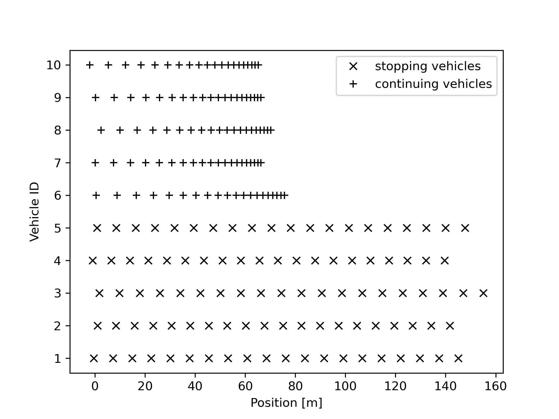

IV-B An example of how to include road user interaction
Fig. 14a shows positions of two vehicles as they approach an intersection, where one vehicle is by the law obliged to stop since the other vehicle approaches from its right hand side. Assume that the stopping vehicle is a target vehicle, whose future position should be predicted. The weighted average model in Sec. II of the target vehicle neglects any effect a vehicle close to the target vehicle has on it. A weighted average model can be formulated to include such effects. In Sec. II substitute “road user” and “target road user” with “traffic situation” and “currently observed traffic situation”, respectively, and substitute and with and . For example, if
- (a)
the state of currently observed traffic situation is , with , and as the current position, speed, and orientation of the target vehicle, as in Sec. II, and as the current position of the other vehicle, where assumes the value if the traffic situation lacks another vehicle than the target vehicle,
- (b)
and with similarly defined,
- (c)
then the resulting model includes effects that the ego-vehicle has on the target vehicle. Notice that the indicator functions amount to selecting from a dataset traffic situations where another vehicle is present when the target traffic situation has another vehicle, and conversely. The possible benefit of such a model is demonstrated on carefully selected real data. The selected data consists of two traffic situation state trajectories and . In the latter traffic situation another vehicle is lacking, thus . The position trajectories of traffic situation trajectories and are shown in Fig. 14a and Fig. 14b, respectively. Trajectory is such that the target vehicle stops to give way to the other vehicle while trajectory is such that the target vehicle drives with approximately constant velocity. Both trajectories are designated as training data while trajectory is also designated as test data. A time index is selected and it is assumed that the currently observed traffic situation state is equal to the traffic situation state . Fig. 15 shows that evaluating model (a)-(c) for a prediction horizon seconds results in sucessfully predicting the future position , while using the model in Sec. II fails. Fig. 16 illustrates the prediction of the model in Sec. II as the varies. It is seen that the predictions are good up until the target vehicle starts waiting at the intersection, which is reasonable since the model has as input only the target vehicle’s current position, speed and orientation, from which it is impossible to know when the target vehicle starts moving again. On the other hand a similar plot for model (a)-(c) shows that this model successfully predicts the target vehicle’s future positions. This is because model (a)-(c) includes as input the position of the other vehicle, which reveals when the target vehicle will start moving again. This indicates that in general, for a larger dataset and when training and test datasets are different, it is expected that including the position of another vehicle gives better performance than what is achieved by the model in Sec. II. Although model (a)-(b) is sufficient for making this argument, the model may be too simple for more general data, since also the speed of the other vehicle may be relevant for determining when the target vehicle starts moving. Such inputs can be included by substituting in (11) with , where and are parameters introduced for additional flexibility.
IV-C Minimum prediction horizon for avoiding collisions
For evaluating the performance scores it is required to relate them to the braking distance of an intelligent vehicle performing predictions. An ideal prediction algorithm should perform well at an arbitrary horizon since it enables an intelligent vehicle to plan far ahead to both avoid collisions and ensure comfort for its passengers. On the other hand, if the application is emergency braking, then the minimum prediction horizon required for an intelligent vehicle to avoid a collision when travelling at some speed can be estimated from Newton’s laws of motion and the standard model for friction. For an initial velocity of the vehicle, the minimum prediction horizon seconds must greater than or equal to the time it takes for the vehicle to come to rest while emergency braking. At an instant of time, the motion of an emergency braking vehicle, wheels locked, driving on a level surface and having mass , acceleration and subject to earth’s gravitational acceleration , can be modeled such that for a coefficient of friction it is that the force on the vehicle is equal to the force of the friction:
| (12) |
By imposing that the initial velocity of the vehicle is and that the velocity after seconds is zero and then solving the resulting equation for , gives that the minimum prediction horizon satisfies
| (13) |
The value of the coefficient of friction depends on factors such as tyre pressure, road type, and weather. According to [25] when a vehicle drives on dry or wet asphalt then and , respectively. Hence, on dry apshalt the minimum prediction horizons for a vehicle moving at typical swedish city speeds of and km/h is and seconds, respectively, and on wet apshalt and seconds. These estimates of the coefficient of friction are based on experiments done in the 1950s. With today’s tires and modern anti-lock braking systems the minimum prediction horizon is expected to be less than the estimates given here.
V Conclusion
A comparison between our formulation of road user position prediction as a weighted average and previously reported state-of-the-art results on real world data shows that further improvement of the formulation is required. This may be explained by the state-of-the-art algorithms including as inputs the positions of every road user surrounding the target road user and including as input also past samples of positions, while our formulation only has as input the target road user’s current position, speed, and orientation. Therefore an example of how to re-formulate our model to include such inputs was presented. The example shows that such input can be included without significantly scaling the complexity of our method. Still, the re-formulation requires selecting from all road users surrounding the target road user the road users that influence the target road user the most, where one possible model of influence is via oppinion dynamics [26]. On the other hand, the state-of-the-arts are based on complex neural networks that have many more, some even with millions more, and less interpretable parameters than the weighted average model. The many parameters of neural networks provide great flexibility for successful application on many types of problems, but their flexibility is also a weakness as demonstrated in [27], where the outputs of neural network image classification algorithms are significantly altered by changing a single pixel in the input images. More examples of such unsafe behavior is found in [28, 29, 30].
Experimental results on real world data indicate that our formulation of road user position prediction as a weighted average produces -second prediction errors comparable to that of the baseline constant velocity model at prediction horizons smaller than approximately seconds for vehicles, bicycles and pedestrians, which indicates that the model needs further adaptations. Hence, if a prediction model is sought for the application of emergency braking in urban environments, speeds less than km/h, then the constant velocity model is preferable due to its simplicity. On the other hand, if a prediction model is meant to support motion planning for autonomous driving applications, where the planned motion is required to be safe and smooth, then longer prediction horizons are required and the weighted average model is preferable over the constant velocity model.
In most cases the weighted average model and a baseline neural network model performs comparably well. For the case of pedestrian position prediction the weighted average model tends to outperform the neural network baseline, while for vehicles the relationship is reversed. Still, our model has only parameters, with clear interpretations, against the thousands of parameters of the neural network model, which are also more difficult to analyze and interpret.
The variation of the -second prediction errors of the weighted average model should be studied as the amount of data increases. As increasing the amount of data used by the model increases the online computational load, techniques for pre-processing newly available data should be explored in order to balance performance improvements and computational load.
If a particular road or side walk in a dataset has few trajectories of road users traversing it, then techniques for automatically switching from the weighted average model to a more suitable model may be required, since the weighted average model performs less well when there are few examples.
In the weighted average model, weights are interpreted as similarity between two road users. It is imposed that similarity decays monotonically as the road users become more different. While we have studied exponential rate of decay, other rates could improve performance. We defined similarity as a comparison between two road users’ current position, speed and orientations, which are factors that do not relate to a unique future position. Including factors based on surrounding road users[22], the geometry of a location[6] and traffic laws[12] could further improve the model. Currently, our method lacks an automatic way of detecting which values of used factors fail to relate to a unique future position, incorporating this could require a probabilistic formulation.
Appendix A Proof of weighted average
Acknowledgment
The authors would like to thank the creators of the freely available python libraries Numpy, Pandas, Matplotlib and Seaborn.
References
- [1] Global Status Report on Road Safety 2018. Geneva: World Health Organization.
- [2] M. Bojarski, D. Del Testa, D. Dworakowski, B. Firner, B. Flepp, P. Goyal, L. D. Jackel, M. Monfort, U. Muller, J. Zhang, et al., “End to end learning for self-driving cars,” arXiv preprint arXiv:1604.07316, 2016.
- [3] I. Batković, “Enabling safe autonomous driving in uncertain environments,” 2022.
- [4] J. Van Brummelen, M. O’Brien, D. Gruyer, and H. Najjaran, “Autonomous vehicle perception: The technology of today and tomorrow,” Transportation research part C: emerging technologies, vol. 89, pp. 384–406, 2018.
- [5] I. Batkovic, M. Zanon, N. Lubbe, and P. Falcone, “A computationally efficient model for pedestrian motion prediction,” in 2018 Eur. Control Conf. (ECC), pp. 374–379.
- [6] V. Karasev, A. Ayvaci, B. Heisele, and S. Soatto, “Intent-aware long-term prediction of pedestrian motion,” in 2016 IEEE Int. Conf. Robot. Automat. (ICRA), pp. 2543–2549.
- [7] E. Rehder, F. Wirth, M. Lauer, and C. Stiller, “Pedestrian prediction by planning using deep neural networks,” in 2018 IEEE Int. Conf. Robot. Automat. (ICRA), pp. 5903–5908.
- [8] J. F. Kooij, F. Flohr, E. A. Pool, and D. M. Gavrila, “Context-based path prediction for targets with switching dynamics,” Int. J. Comput. Vision, vol. 127, no. 3, pp. 239–262, 2019.
- [9] R. Q. Mínguez, I. P. Alonso, D. Fernández-Llorca, and M. A. Sotelo, “Pedestrian path, pose, and intention prediction through gaussian process dynamical models and pedestrian activity recognition,” IEEE Trans. Intell. Transp. Syst., vol. 20, no. 5, pp. 1803–1814, 2018.
- [10] Y. F. Chen, M. Liu, and J. P. How, “Augmented dictionary learning for motion prediction,” in 2016 IEEE Int. Conf. Robot. Automat. (ICRA), 2016, pp. 2527–2534.
- [11] B. Völz, H. Mielenz, I. Gilitschenski, R. Siegwart, and J. Nieto, “Inferring pedestrian motions at urban crosswalks,” IEEE Trans. Intell. Transp. Syst., vol. 20, no. 2, pp. 544–555, 2018.
- [12] M. Koschi and M. Althoff, “Set-based prediction of traffic participants considering occlusions and traffic rules,” IEEE Trans. Intell. Veh., vol. 6, no. 2, pp. 249–265, 2021.
- [13] S. Carrasco, D. F. Llorca, and M. Sotelo, “Scout: Socially-consistent and understandable graph attention network for trajectory prediction of vehicles and vrus,” in 2021 IEEE Intell. Vehicles Symp. (IV).
- [14] A. Alahi, K. Goel, V. Ramanathan, A. Robicquet, L. Fei-Fei, and S. Savarese, “Social lstm: Human trajectory prediction in crowded spaces,” in Proc. IEEE Conf. Comput. Vision Pattern Recognit. (CVPR), 2016, pp. 961–971.
- [15] A. Gupta, J. Johnson, L. Fei-Fei, S. Savarese, and A. Alahi, “Social gan: Socially acceptable trajectories with generative adversarial networks,” in Proc. IEEE Conf. Comput. Vision Pattern Recognit. (CVPR), June 2018.
- [16] X. Li, X. Ying, and M. C. Chuah, “Grip++: Enhanced graph-based interaction-aware trajectory prediction for autonomous driving,” arXiv preprint arXiv:1907.07792, 2019.
- [17] H. Cheng, W. Liao, M. Y. Yang, B. Rosenhahn, and M. Sester, “Amenet: Attentive maps encoder network for trajectory prediction,” ISPRS J. Photogram. Remote Sens., vol. 172, pp. 253–266, 2021.
- [18] H. Cheng, W. Liao, X. Tang, M. Y. Yang, M. Sester, and B. Rosenhahn, “Exploring dynamic context for multi-path trajectory prediction,” in 2021 IEEE Int. Conf. Robot. Automat. (ICRA), pp. 12 795–12 801.
- [19] A. Toytziaridis, P. Falcone, and J. Sjöberg, “A data-driven markovian framework for multi-agent pedestrian collision risk prediction,” in 2019 IEEE Intell. Transp. Syst. Conf. (ITSC).
- [20] E. A. Nadaraya, “On estimating regression,” Theory of Probability & Its Applications, vol. 9, no. 1, pp. 141–142, 1964.
- [21] C. G. Atkeson, A. W. Moore, and S. Schaal, “Locally weighted learning,” Lazy learning, pp. 11–73, 1997.
- [22] R. F. Martin and D. R. Parisi, “Data-driven simulation of pedestrian collision avoidance with a nonparametric neural network,” Neurocomputing, vol. 379, pp. 130–140, 2020.
- [23] J. Bock, R. Krajewski, T. Moers, S. Runde, L. Vater, and L. Eckstein, “The ind dataset: A drone dataset of naturalistic road user trajectories at german intersections,” in 2020 IEEE Intell. Vehicles Symp. (IV), pp. 1929–1934.
- [24] T. Hastie, R. Tibshirani, and J. Friedman, The elements of statistical learning. Springer, 2009.
- [25] J. Y. Wong, Theory of ground vehicles. John Wiley & Sons, 2008.
- [26] C.-J. Heiker and P. Falcone, “Collective decision making using attractive and repulsive forces in markovian opinion dynamics,” arXiv:2203.11116, 2022.
- [27] J. Su, D. V. Vargas, and K. Sakurai, “One pixel attack for fooling deep neural networks,” IEEE Transactions on Evolutionary Computation, vol. 23, no. 5, pp. 828–841, 2019.
- [28] D. J. Miller, Z. Xiang, and G. Kesidis, “Adversarial learning targeting deep neural network classification: A comprehensive review of defenses against attacks,” Proceedings of the IEEE, vol. 108, no. 3, pp. 402–433, 2020.
- [29] Z. Kong, J. Xue, Y. Wang, L. Huang, Z. Niu, and F. Li, “A survey on adversarial attack in the age of artificial intelligence,” Wireless Communications and Mobile Computing, vol. 2021, 2021.
- [30] X. Huang, D. Kroening, W. Ruan, J. Sharp, Y. Sun, E. Thamo, M. Wu, and X. Yi, “A survey of safety and trustworthiness of deep neural networks: Verification, testing, adversarial attack and defence, and interpretability,” Computer Science Review, vol. 37, p. 100270, 2020.
- [31] K. B. Petersen and M. S. Pedersen, “The matrix cookbook (version: November 15, 2012),” 2012.
| Michael Shell Biography text here. |
| John Doe Biography text here. |
| Jane Doe Biography text here. |