Graph Representation Learning via Aggregation Enhancement

Maxim Fishman Affiliation: Technion Affiliation: Habana Labs Chaim Baskin Affiliation: Technion Correspondence to: chaimbaskin@cs.technion.ac.il Evgenii Zheltonozhskii Affiliation: Technion Almog David Affiliation: Technion Ron Banner Affiliation: Habana Labs Avi Mendelson Affiliation: Technion

Abstract

Graph neural networks (GNNs) have become a powerful tool for processing graph-structured data but still face challenges in effectively aggregating and propagating information between layers, which limits their performance. We tackle this problem with the kernel regression (KR) approach, using KR loss as the primary loss in self-supervised settings or as a regularization term in supervised settings. We show substantial performance improvements compared to state-of-the-art in both scenarios on multiple transductive and inductive node classification datasets, especially for deep networks. As opposed to mutual information (MI), KR loss is convex and easy to estimate in high-dimensional cases, even though it indirectly maximizes the MI between its inputs. Our work highlights the potential of KR to advance the field of graph representation learning and enhance the performance of GNNs. The code to reproduce our experiments is available at https://github.com/Anonymous1252022/KR_for_GNNs.

Keywords:

Graph Neural Networks

^†^†affiliationnotice: Equal contribution

1 Introduction

Refer to caption — Figure 1: (a) A schematic representation of GIRL algorithm, where $\mathcal{L}_{SSL}$ is the sum of KR losses between $\mathcal{G}_{in}$ and $\mathcal{G}_{out}$ of each GNN layer $g_{\theta_{\ell}}$ . (b) A schematic representation of KR. By minimizing KR loss between $\mathbf{h}_{i}^{(\ell)}$ (the node features of the output graph) and $\mathbf{h}_{i}^{(\ell-1)}$ (node features of the input graph) as well as between $\mathbf{h}_{i}^{(\ell)}$ and $\quantity{ \mathbf{h}_{j_k}^{(\ell- 1)} }$ (direct neighbors of $\mathbf{h}_{i}^{(\ell-1)}$ ), we improve the information propagation and indirectly maximize MI.

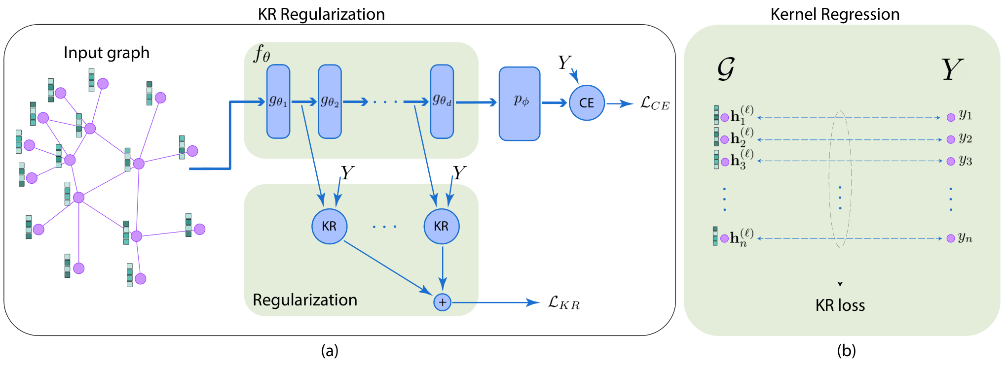
Graph neural networks (Gori et al. 2005; Scarselli et al. 2008; Kipf and Welling 2017, GNNs,) have become a popular tool for machine learning with graphs (Wu et al. 2019; Ribeiro et al. 2017b; Shapson-Coe et al. 2021; Cvitkovic 2020; Sen et al. 2008; Bloemheuvel et al. 2021). GNNs employ a message-passing mechanism (Gilmer et al. 2017), iteratively updating node representations based on information from their neighbors to learn representations of graph-based data. Despite their success, GNNs still face challenges in effectively aggregating and propagating information between graph nodes. For example, graph convolution networks (Kipf and Welling 2017, GCNs,) aggregate information from neighboring nodes homogeneously without the ability to selectively choose aggregation pathways. Graph attention networks (Veličković et al. 2018, GATs,) address this issue by incorporating a self-attention mechanism (Vaswani et al. 2017) into aggregation but are still prone to the depth problem (Alon and Yahav 2021), the lack of ability to propagate information between distant nodes in the graph effectively.

To overcome the challenges of information aggregation, some researchers (Peng et al. 2020b; Bandyopadhyay et al. 2020; Sun et al. 2020; Veličković et al. 2018) have proposed using mutual information (MI) maximization techniques. MI estimation, however, can be a formidable task, especially for high-dimensional random variables (Paninski 2003), as it requires estimating high-dimensional probability density functions from a limited number of samples. This can be a significant limitation for deep learning approaches such as GNNs, which often involve high-dimensional representations.

In this paper, we propose utilizing the kernel regression (Aravkin et al. 2013, KR,) method as a means of enhancing graph representation learning in both supervised and self-supervised settings. KR is a technique that relies on reproducing kernel Hilbert space (Aronszajn 1950, RKHS,) embedding to identify non-linear relationships between pairs of random variables. We propose using the KR loss as surrogate for MI estimation. We present theoretical and empirical evidence that minimization of KR loss corresponds to the maximization of MI. As a result, the simplicity of KR loss estimation, coming from its convex nature, makes it a valuable alternative to direct MI maximization. Our experimental results demonstrate that incorporating the KR loss between graph representations and the target as a regularization term (Figure 2) during training of deep GNNs in a supervised setting can significantly improve performance. Furthermore, we introduce a new self-supervised algorithm for graph representation learning called Graph Information Representation Learning (GIRL), which is based on KR and surpasses previous state-of-the-art contrast-based algorithms. The algorithm is shown in Figure 1. We employ KR loss minimization between the input and output of each GNN layer for learning representations.

Our main contributions are as follows:

•

We provide evidence that KR loss minimization leads to MI maximization. The convexity of KR makes it a more practical alternative to MI estimation, which can be complex, especially for high-dimensional random variables.
•

We show that KR-based regularization in supervised training of deep GNNs improves information aggregation.
•

We develop a self-supervised graph representation learning algorithm based on KR, named GIRL, which significantly outperforms previous state-of-the-art contrast-based algorithms.

2 Related Work

In this section, we briefly overview previous works on information propagation in GNNs, MI maximization, and self-supervised graph representation learning.

MI Maximization and KR

MI is a measure of dependency between two random variables and is a cornerstone of information theory. The MI maximization principle is used widely in deep learning (Peng et al. 2020b; Bandyopadhyay et al. 2020; Sun et al. 2020). MI estimation, nevertheless, remains difficult, especially for high-dimensional random variables (Paninski 2003). Kleinman et al. 2021 addressed this issue by introducing a notion of usable information based on MI, which is contained in the representation learned by a deep network. In many recent works, MI is estimated via MINE (Belghazi et al. 2018) or its improvement, MI-NEE (Chan et al. 2019), which involves a lot of additional parameters that must be learned for correct MI estimation. Other approaches for MI estimation utilize finding lower bounds using variational Bayesian methods (Alemi et al. 2016; Alemi et al. 2017; Barber and Agakov 2003; Blei et al. 2017). We eliminate explicit MI estimation in our work by turning to the KR method, a popular approach in the machine learning toolbox (Hofmann et al. 2008; Muandet et al. 2017; Klebanov et al. 2021). Primarily, the KR technique has been used for finding non-linear relations between random variables by mapping their distributions into RKHS (Aronszajn 1950), where the relations turn to be linear. Instead of finding a non-linear relation between two random variables, we use the KR loss as a proxy for MI.

Information Propagation to Distant Nodes

Li et al. 2018 showed that the GCN model is a particular form of Laplacian smoothing and raised the concern of over-smoothing, the inability to distinguish between node representations in deeper layers, which prevents information propagation to distant nodes. Alon and Yahav 2021 proposed an alternative explanation to the problem of information propagation: GNNs are susceptible to a bottleneck when aggregating messages across a long path. This bottleneck causes the over-squashing of exponentially growing information into fixed-size vectors. Topping et al. 2021 introduced a new edge-based combinatorial curvature and proved that negatively curved edges are responsible for the over-squashing issue. Rusch et al. 2022 proposed a gradient gating framework that alleviates the over-smoothing problem. We demonstrate that KR-based regularization leads to better information aggregation in GNNs, which improves the accuracy of deep networks.

Self-Supervised Learning in GNNs

According to Liu et al. 2022, graph self-supervised learning methods can be roughly split into four categories: generation-based, auxiliary property-based, contrast-based and hybrid. The generation-based methods aim to reconstruct the input data, and can be divided into two sub-categories: feature generation that learns to reconstruct the feature information of graphs (Jin et al. 2020a; Wang et al. 2017; Manessi and Rozza 2020; Park et al. 2019) and structure generation that learns to reconstruct the topological structure information of graphs (Hasanzadeh et al. 2019; Pan et al. 2018; Kim and Oh 2022; Hu et al. 2019; Zhu et al. 2020a). In auxiliary property-based methods, the auxiliary properties are extracted from the graph freely; afterward, the decoder aims to predict the extracted properties (Zhu et al. 2020c; Peng et al. 2020a; Jin et al. 2020b; Lin et al. 2021; Kang et al. 2021). Contrastive methods can be classified by augmentation techniques: node feature masking (Zhu et al. 2020b; You et al. 2020; Hu et al. 2020b; Jin et al. 2020a; Jin et al. 2021), node feature shuffling (Veličković et al. 2018; Opolka et al. 2019; Ren et al. 2019), edge modification (Hu et al. 2020c; Zhu et al. 2020a; Zhang et al. 2020; Zeng and Xie 2020), graph diffusion (Gasteiger et al. 2019; Hassani and Khasahmadi 2020), and sub-graph sampling (Jiao et al. 2020). Finally, hybrid methods (Chen et al. 2021; Wan et al. 2020; Fan et al. 2021; Xu et al. 2021; Jing et al. 2021; Zheng et al. 2021; Roy et al. 2021; Thakoor et al. 2021) combine one or more of the aforementioned methods.

The most common self-supervised methods are generally contrastive, based on MI maximization and data augmentation techniques. We propose GIRL, a novel self-supervised learning algorithm that does not require augmentations or a decoder for MI estimation.

3 Background

This section introduces the notation used throughout the paper and defines a probabilistic model for a single intermediate GNN layer. We also define the random variables involved in the information aggregation process.

3.1 Basic Notations

This paper focuses on node-attributed graphs and node classification tasks for evaluating both supervised (as a primary task) and self-supervised learning (as a downstream task) performance. We use the notation $[n]=\quantity{ 1, 2, \dots, n }$ throughout the paper.

A node-attributed graph is a tuple $\mathcal{G}=(\quantity{\mathbf{x}_i}_{i\in[n]},\mathcal{E})$ , where $\quantity{\mathbf{x}_i}_{i\in[n]}\subset\mathbb{R}^{d_{1}}$ are the node features and $\mathcal{E}\subseteq[n]\times[n]$ ( $|\mathcal{E}|=m$ ) is the set of edges. The set of direct neighboring nodes for node $i$ is denoted as $\mathcal{N}(i)$ .

The node classification task involves predicting the label $y_{i}\in\mathcal{Y}$ for each node $i\in[n]$ , where $\mathcal{Y}$ is the set of possible labels. The graph encoder $f_{\theta}$ , parameterized by $\theta$ , processes the node-attributed graph $\mathcal{G}$ and generates node representations (embeddings) $\quantity{\mathbf{h}_i}_{i\in[n]}\subset\mathbb{R}^{d_{2}}$ :

\displaystyle f_{\theta}(\mathcal{G})=(\{\mathbf{h}_{i}\}_{i\in[n]},\mathcal{E}).

(1)

The classifier $p_{\phi}$ , parameterized by $\phi$ , takes these embeddings as inputs and produces logits. Finally, the cross-entropy (CE) loss $\mathcal{L}_{\text{CE}}$ is optimized. The node classification problem is defined as:

\displaystyle\theta^{*},\phi^{*}=\argmin_{\theta,\phi}\frac{1}{n}\sum_{j\in[n]}\mathcal{L}_{\text{CE}}(p_{\phi}([f_{\theta}(\mathcal{G})]_{j}),y_{j}),

(2)

where $[\cdot]_{j}$ is a choice function defined as $[(\{\mathbf{h}_{i}\}_{i\in[n]},\mathcal{E})]_{j}=\mathbf{h}_{j}$ .

The graph encoder $f_{\theta}$ is typically composed of multiple GNN layers, represented as:

\displaystyle f_{\theta}=g_{\theta_{d}}\circ\cdots\circ g_{\theta_{\ell}}\circ\cdots\circ g_{\theta_{1}},

(3)

where $d$ is the depth of the network, $g_{\theta_{\ell}}$ is an intermediate GNN layer:

\displaystyle g_{\theta_{\ell}}(\{\mathbf{h}^{(\ell-1)}_{i}\}_{i\in[n]},\mathcal{E})=(\{\mathbf{h}^{(\ell)}_{i}\}_{i\in[n]},\mathcal{E}),

(4)

and $\theta=\quantity{\theta_{1}, \dots, \theta_{\ell}, \dots, \theta_{d}}$ are the network parameters. Each GNN layer $g_{\theta_{\ell}}$ follows a message passing scheme (Gilmer et al. 2017), where information is only aggregated from direct neighboring nodes, as visualized in Figure 3. As a result, the depth of the aggregation is equal to $d$ , the number of layers in the graph encoder $f_{\theta}$ .

In the self-supervised setting, the goal is to learn a meaningful graph representation without access to the node labels $\{y_{i}\}_{i\in[n]}$ . To achieve this, a self-supervised algorithm is used to learn the parameters $\theta^{*}$ of graph encoder $f_{\theta}$ . The quality of the learned representations $\{\mathbf{h}_{i}\}_{i\in[n]}$ is then evaluated by training a network for the downstream task (in our case, node classification), with the (frozen) extracted features as input and node labels as outputs:

\displaystyle\phi^{*}=\argmin_{\phi}\frac{1}{n}\sum_{i\in[n]}\mathcal{L}_{\text{CE}}(p_{\phi}([f_{\theta^{*}}(\mathcal{G})]_{i}),y_{i}).

(5)

3.2 Probabilistic Model of Information Aggregation

We now formalize the information aggregation and propagation processes in GNNs using random variables. Given an intermediate graph representation, i.e., the output of layer $g_{\theta_{\ell}}$ as shown Figure 3, $(\{\mathbf{h}^{(\ell)}_{i}\}_{i\in[n]},\mathcal{E})$ and the node labels ${y_{i}}$ , we define the random variables for the node features, node neighborhood features, and node labels: $H^{(\ell)}$ , $Z^{(\ell)}$ , and $Y$ , correspondingly. For $j$ uniformly distributed over $[n]$ , $H^{(\ell)}=\mathbf{h}^{(\ell)}_{j}$ , $Z^{(\ell)}$ is a vector uniformly distributed over $\{\mathbf{h}^{(\ell)}_{k}\}_{k\in\mathcal{N}(j)}$ , and $Y=y_{j}$ . The three variables are correlated, i.e., they share the same sampled $j$ .

At each layer $g_{\theta_{\ell}}$ , information flows from both $H^{(\ell-1)}$ and $Z^{(\ell-1)}$ to $H^{(\ell)}$ . The random variable $Z^{(\ell-1)}$ contains the information from the neighborhood and is vital for the aggregation process.

4 Aggregation Enhancement

Based on definitions provided in Section 3, we present MI- and KR-based approaches for information aggregation in supervised and self-supervised settings.

4.1 MI Approach

The ability of the classifier $p_{\phi}$ to learn from the node representations $\{\mathbf{h}_{i}\}_{i\in[n]}$ depends on the mutual information $I(H^{(d)};Y)$ (the random variable of node representations $H^{(d)}$ was defined in Section 3.2). When $I(H^{(d)};Y)=0$ , the random variables $H^{(d)}$ and $Y$ are statistically independent, and it impossible to learn $Y$ from $H^{(d)}$ . On the other hand, when a deterministic continuous map from $H^{(d)}$ to $Y$ exists, the random variables $H^{(d)}$ and $Y$ are dependent, resulting in a high value of the mutual information $I(H^{(d)};Y)$ . As a result, maximization of the total mutual information $\sum_{\ell\in[d]}I(H^{(\ell)};Y)$ along with the supervised loss minimization enhances information aggregation.

In self-supervised representation learning, it is unknown which information should be preserved in the node embeddings to perform the downstream task well (node classification). In this case, we aim to retain as much information as possible in the intermediate node representations. This can be done by maximization of the following quantity:

\displaystyle\sum_{l\in[d]}\quantity(I(H^{(\ell)}; H^{(\ell-1)}) + I(H^{(\ell)}; Z^{(\ell-1)}))

(6)

Estimating mutual information from samples, however, can be difficult, especially for high-dimensional random vectors. We propose using kernel regression (Aravkin et al. 2013, KR,) as an alternative, which is easier to estimate and does not require additional learnable parameters.

4.2 The KR Approach

In the following, we redefine KR loss $\rho$ and convince the reader that $\rho$ minimization leads to MI maximization. Next, we demonstrate the KR loss minimization technique for aggregation enhancement in GNNs.

As previously noted, the ability to learn node labels $\{y_{i}\}_{i\in[n]}$ from node representations $\{\mathbf{h}^{(d)}_{i}\}_{i\in[n]}$ depends on the existence of a continuous map from $H^{(d)}$ to $Y$ . Let $X$ and $Y$ be two random variables with values in $\mathbb{R}^{\ell}$ and $\mathbb{R}^{m}$ , respectively. We define

\displaystyle\mathcal{C}_{X}=\quantity{ f(X) \;|\; f:\mathbb{R}^{\ell} \rightarrow\mathbb{R}^m \text{ is continuous function} },

(7)

and evaluate the distance between the random variable $Y$ and the set $\mathcal{C}_{X}$ :

\displaystyle\rho(Y|X)=\inf_{Z\in\mathcal{C}_{X}}d(Y,Z),

(8)

where $d$ is some distance between two random variables, e.g., a metric induced by the $L_{p}$ norm, $\mathbb{E}[\absolutevalue{X}^{p}]^{\nicefrac{{1}}{{p}}}$ .

Theorem 4.1.

For any pair of random variables $X$ and $Y$ , $\rho(Y|X)=0$ if and only if $I(X;Y)=H(Y)$ , where $I(X;Y)$ is the MI between $X$ and $Y$ , and $H(Y)$ is the entropy of $Y$ .

The proof of Theorem 4.1 is given in Section A.1.

The consequence of Theorem 4.1 is that for a fixed $Y$ , finding random variable $X$ such that $\rho(Y|X)=0$ is equivalent to finding an $X$ that maximizes the $I(X;Y)$ , because $I(X;Y)\leq H(Y)$ for any two random variables $X$ and $Y$ . Additionally, the empirical result given in Figure C.2 presents evidence that KR loss minimization leads to MI maximization.

The following theorem shows how KR loss $\rho$ can be efficiently estimated.

Theorem 4.2.

Given a collection of points $\{\mathbf{x}_{i}\}_{i\in[n]}$ and $\{\mathbf{y}_{i}\}_{i\in[n]}$ sampled i.i.d. from $X$ and $Y$ , respectively, the empirical estimation of distance $\rho(Y|X)$ is given by

\displaystyle\hat{\rho}(Y|X)=\frac{1}{m}\sum_{i\in[m]}\left(\left(\frac{1}{n}\sum_{k\in[n]}\left|\sum_{j\in[n]}(\mathbb{I}-\Pi)_{kj}\mathbf{y}_{j}\right|^{p}\right)^{\nicefrac{{1}}{{p}}}\right)_{i}

(9)

where $\Pi$ is an orthogonal projection onto $\imaginary(K)$ and $K_{ij}=\exp\left(-\frac{\norm{\mathbf{x}_i - \mathbf{x}_j}^{2}}{2\sigma^{2}}\right)$ is a Gram matrix.

We provide the proof of Theorem 4.2 in Section A.2 and experiments on synthetic data in Appendix C.

Turning back to the graph supervised setting, we propose to replace maximization of total mutual information $\sum_{l\in[d]}I(H^{(l)};Y)$ by minimization of $\sum_{l\in[d]}\hat{\rho}(Y|H^{(l)})$ , as follows:

	$\displaystyle\theta^{},\phi^{}=\argmin_{\theta,\phi}\frac{1}{n}\sum_{j\in[n]}\mathcal{L}_{\text{CE}}(p_{\phi}([f_{\theta}(\mathcal{G})]_{j}),y_{j})+$		(10)
	$\displaystyle+\lambda\sum_{l\in[d]}\hat{\rho}(Y\|H^{(l)})$		(11)

We also propose a self-supervised graph representation learning algorithm called GIRL (Graph Information Representation Learning). In the self-supervised setting, our goal is to transfer as much information as possible from the random variables $H^{(\ell-1)}$ and $Z^{(\ell-1)}$ to $H^{(l)}$ in each layer $\ell\in[d]$ of the graph encoder $f_{\theta}$ . To do this, we seek to minimize the total distance $\rho(H^{(l-1)}|H^{(l)})+\rho(Z^{(l-1)}|H^{(l)})$ between the current layer node embeddings and previous layer embeddings of the node and its neighbors. This is achieved by solving the following optimization problem:

\displaystyle\theta^{*}=\argmin_{\theta}\sum_{l\in[d]}\left(\hat{\rho}(H^{(l-1)}|H^{(l)})+\hat{\rho}(Z^{(l-1)}|H^{(l)})\right)

(12)

The algorithm is provided in Appendix B and illustrated in Figure 1.

5 Experiments

Figure 4: Reddit: The drop in training and test accuracy, along with the GNN depth extension.

Figure 5: PPI: The drop in training and test accuracy, along with the GNN depth extension.

Depth	Method	Accuracy
Depth	Method	Reddit	Reddit2	ogbn-arxiv	ogbn-products	PPI	Texas	Actor
3	None	92.9 $\pm$ 0.1	93.0 $\pm$ 0.1	66.2 $\pm$ 0.3	75.5 $\pm$ 0.3	86.6 $\pm$ 0.1	77.8 $\pm$ 1.2	34.2 $\pm$ 0.8
	WD	92.9 $\pm$ 0.1	92.9 $\pm$ 0.1	65.9 $\pm$ 0.3	75.6 $\pm$ 0.3	85.9 $\pm$ 0.1	76.2 $\pm$ 2.3	34.4 $\pm$ 0.6
	+FA	92.6 $\pm$ 0.1	92.0 $\pm$ 0.1	65.8 $\pm$ 0.4	74.3 $\pm$ 0.1	85.8 $\pm$ 0.1	73.0 $\pm$ 3.3	33.6 $\pm$ 1.3
	KR (ours)	93.0 $\pm$ 0.1	93.1 $\pm$ 0.1	66.2 $\pm$ 0.4	75.6 $\pm$ 0.2	86.8 $\pm$ 0.1	77.3 $\pm$ 2.3	35.1 $\pm$ 0.3
9	None	91.9 $\pm$ 0.2	90.3 $\pm$ 0.6	66.4 $\pm$ 0.5	75.8 $\pm$ 0.3	83.9 $\pm$ 0.1	62.7 $\pm$ 7.0	31.8 $\pm$ 3.9
	WD	91.5 $\pm$ 0.3	89.7 $\pm$ 1.1	65.3 $\pm$ 0.4	75.3 $\pm$ 0.5	82.2 $\pm$ 0.2	68.1 $\pm$ 3.0	31.3 $\pm$ 1.5
	+FA	92.8 $\pm$ 0.1	90.6 $\pm$ 0.6	66.9 $\pm$ 0.1	76.3 $\pm$ 0.1	83.7 $\pm$ 0.1	37.8 $\pm$ 11.0	32.7 $\pm$ 0.9
	KR (ours)	92.6 $\pm$ 0.1	92.1 $\pm$ 0.1	67.2 $\pm$ 0.3	75.8 $\pm$ 0.1	85.0 $\pm$ 0.1	75.7 $\pm$ 2.7	32.8 $\pm$ 0.4
18	None	89.2 $\pm$ 0.3	33.3 $\pm$ 25.7	64.7 $\pm$ 0.2	73.2 $\pm$ 0.3	76.9 $\pm$ 1.5	63.8 $\pm$ 1.5	23.8 $\pm$ 2.1
	WD	88.4 $\pm$ 0.2	14.9 $\pm$ 0.0	63.4 $\pm$ 0.2	72.4 $\pm$ 0.9	74.3 $\pm$ 0.1	61.1 $\pm$ 8.5	24.9 $\pm$ 0.9
	+FA	82.5 $\pm$ 1.7	52.6 $\pm$ 21.7	57.2 $\pm$ 1.9	63.5 $\pm$ 7.1	78.7 $\pm$ 0.1	62.2 $\pm$ 12.1	24.6 $\pm$ 1.1
	KR (ours)	91.4 $\pm$ 0.4	76.4 $\pm$ 1.0	65.7 $\pm$ 0.3	74.6 $\pm$ 0.4	80.2 $\pm$ 0.2	67.6 $\pm$ 2.4	30.2 $\pm$ 1.1

Table 1: The performance of the model with different depths, both with and without weight decay (WD), fully-adjacent layer (+FA) (Alon and Yahav 2021), and kernel regression loss (KR). The table is divided into three blocks based on depth, with the best results for each depth highlighted in bold.

(a) Transductive
Dataset	DGI	GRACE	BGCL	BGRL	GraphMAE	GIRL (ours)
Cora	82.3 $\pm$ 0.6	84.0 $\pm$ 0.1	83.8 $\pm$ 0.3	-	84.2 $\pm$ 0.4	88.3 $\pm$ 0.1
Citeseer	71.8 $\pm$ 0.7	72.1 $\pm$ 0.5	72.7 $\pm$ 0.3	-	73.4 $\pm$ 0.4	79.1 $\pm$ 0.3
Pubmed	76.8 $\pm$ 0.6	86.7 $\pm$ 0.1	-	-	81.1 $\pm$ 0.4	89.0 $\pm$ 0.0
DBLP	-	84.2 $\pm$ 0.1	-	-	-	85.9 $\pm$ 0.1
Amazon-Photos	91.6 $\pm$ 0.2	92.2 $\pm$ 0.2	92.5 $\pm$ 0.2	93.2 $\pm$ 0.3	-	95.6 $\pm$ 0.1
WikiCS	75.4 $\pm$ 0.1	80.1 $\pm$ 0.5	-	80.0 $\pm$ 0.1	-	83.3 $\pm$ 0.0
Amazon-Computers	84.0 $\pm$ 0.5	89.5 $\pm$ 0.4	-	90.3 $\pm$ 0.2	-	91.8 $\pm$ 0.0
Coauthor CS	92.2 $\pm$ 0.6	91.1 $\pm$ 0.2	-	93.3 $\pm$ 0.1	-	94.5 $\pm$ 0.0
Coauthor Physics	94.5 $\pm$ 0.5	-	-	95.7 $\pm$ 0.1	-	96.6 $\pm$ 0.0

(b) Inductive
Dataset	DGI	GRACE	BGRL	SimGRACE	GraphMAE	GIRL (ours)
PPI	63.8 $\pm$ 0.2	66.2 $\pm$ 0.1	70.5 $\pm$ 0.1	70.3 $\pm$ 1.2	74.5 $\pm$ 0.3	87.9 $\pm$ 0.1
Reddit	94.0 $\pm$ 0.1	94.2 $\pm$ 0.0	-	-	-	92.1 $\pm$ 0.0
Reddit2	-	91.7 $\pm$ 0.0^∗	-	-	96.0 $\pm$ 0.1	92.1 $\pm$ 0.0
ogbn-arxiv	-	69.0 $\pm$ 0.3^∗	71.6 $\pm$ 0.1	-	71.75 $\pm$ 0.17	71.8 $\pm$ 0.2
ogbn-products	-	68.1 $\pm$ 0.1^∗	-	-	-	71.5 $\pm$ 0.3

(c) Heterophilic
Dataset	DGI	SELENE	GIRL (ours)
Texas	54.1	64.3	75.7
Actor	27.2	34.1	34.2
USA-Airports	31.1	56.5	65.1

(d) Graph Property Prediction
Dataset	InfoGraph	GraphCL	JOAO	JOAOv2	SimGRACE	GraphMAE	GIRL (ours)
NCI1	77.9 $\pm$ 1.1	77.9 $\pm$ 0.4	78.1 $\pm$ 0.5	78.4 $\pm$ 0.5	79.1 $\pm$ 0.4	80.4 $\pm$ 0.3	80.6 $\pm$ 0.1
PROTEINS	74.4 $\pm$ 0.3	74.4 $\pm$ 0.5	74.6 $\pm$ 0.4	74.1 $\pm$ 1.1	75.4 $\pm$ 0.1	75.3 $\pm$ 0.4	75.6 $\pm$ 0.1
DD	72.9 $\pm$ 1.8	78.6 $\pm$ 0.4	77.3 $\pm$ 0.5	77.4 $\pm$ 1.2	77.4 $\pm$ 1.1	-	78.9 $\pm$ 0.1
MUTAG	89.0 $\pm$ 1.1	86.8 $\pm$ 1.3	87.4 $\pm$ 1.0	87.7 $\pm$ 0.8	89.0 $\pm$ 1.3	88.2 $\pm$ 1.3	89.5 $\pm$ 0.1

Table 2: Summary of the classification accuracy for transductive, inductive, heterophilic, and graph property prediction datasets, with their standard deviations. These results are averaged over ten training runs with different seeds; the best results are highlighted in bold. Results reproduced using GRACE with the same model as with GIRL are marked with a ^∗.

Figure 6: Comparison of downstream task test accuracy of the self-supervised setup and random initial setup. In both cases, the network was initialized randomly, and only in the self-supervised case, was the network trained with our self-supervised objective. Each column refers to a different dataset. Each row corresponds to a different GNN layer type.

The main purpose of the following experiments is to demonstrate empirically that the KR loss minimization technique can be used for aggregation enhancement in GNNs. We split the experiments into two settings: supervised and self-supervised. In the supervised setting, we show that KR loss minimization leads to better aggregation of information, which helps to alleviate the depth problem. In the self-supervised setting, we compare our algorithm GIRL (Figure 1) with other self-supervised methods. All experiments were done on Nvidia RTX A6000 GPUs.

5.1 Datasets

We conducted experiments on multiple transductive (Cora, CiteSeer, Pubmed (Yang et al. 2016), DBLP (Fu et al. 2020), Amazon-Photos (Shchur et al. 2018), WikiCS (Mernyei and Cangea 2020), Amazon-Computers, Coauthor CS and Coauthor Physics (Shchur et al. 2018)), inductive (Reddit (Hamilton et al. 2017b), Reddit2 (Zeng et al. 2019), PPI (Zitnik and Leskovec 2017), ogbn-arxiv, ogbn-products (Hu et al. 2020a)), heterophily (Texas, Actor (Pei et al. 2020) and USA-Airports (Ribeiro et al. 2017a)) and graph property prediction datasets (NCI1, PROTEINS, DD and MUTAG (Morris et al. 2020)). The detailed information about the datasets can be found in Table C.2.

5.2 Supervised Setting

First, we study the effect of KR loss on the depth problem in GNNs, where the performance of the GNNs diminishes as they get deeper. We show that the accuracy of deep GNNs can be improved through auxiliary KR loss, as described in Equation 10.

5.2.1 Experimental setup

To demonstrate the depth problem, we trained a GNN model with different depths. The model consists of two consecutive blocks: an encoder $f_{\theta}$ and a decoder $p_{\phi}$ . The encoder $f_{\theta}$ has $d$ SAGE layers (Hamilton et al. 2017a), where $d\in\{3,6,9,12,15,18\}$ . In the +FA configuration, the last layer in $f_{\theta}$ is replaced by a fully-adjacent layer (Alon and Yahav 2021). The decoder $p_{\phi}$ includes three fully connected layers. All but the last model layers are followed by a ReLU activation and a dropout with a drop probability of 0.1. For all datasets, we used a cluster data loader (Chiang et al. 2019).

5.2.2 Results

The results of this experiment are summarized in Table 1 and Figures 4 and 5. As shown in Figures 4 and 5, both training and test accuracy decrease with increasing depth, but the generalization gap does not increase. This suggests that overfitting is not a significant issue in this case. Instead, we observe the depth problem. Table 1 shows that adding weight decay regularization to the supervised loss leads to a degradation in test accuracy, which is expected in the absence of overfitting. When, however, the KR loss is optimized alongside the supervised loss (10), we see a significant improvement in test accuracy at all depths. In the majority of cases, the KR loss optimization technique surpasses the +FA method (Alon and Yahav 2021). We attribute the improvement in performance to the enhanced information aggregation at each GNN layer resulting from the minimization of the KR loss.

5.3 Self-Supervised Setting

We evaluate the effectiveness of our self-supervised graph representation learning method, GIRL, on various node classification tasks (transductive and inductive settings, as well as high-heterophily graphs) and graph classification tasks. We compare our results to those obtained by several existing self-supervised methods: DGI (Veličković et al. 2018), GRACE (Zhu et al. 2020b), BGCL (Hasanzadeh et al. 2021), BGRL (Thakoor et al. 2021) GraphCL (You et al. 2020), JOAO, JOAOv2 (You et al. 2021), SimGRACE (Xia et al. 2022), SELENE (Zhong et al. 2022) and GraphMAE (Hou et al. 2022).

5.3.1 Experimental setup

We used a cluster data loader (Chiang et al. 2019) to load the inductive datasets, while the transductive and heterophily datasets were loaded as whole graphs. We used the unsupervised representation learning (URL) setting (Liu et al. 2022) and applied GIRL (Figure 1) to a simple GNN encoder $f_{\theta}$ with GCN layers (Kipf and Welling 2017) to obtain $\theta^{*}$ . The quality of the learned encoder $f_{\theta^{*}}$ was then evaluated by training a decoder $p_{\phi}$ , as described in Section 3.1.

5.3.2 Results

The results averaged over ten training runs with different seeds are summarized in Table 2. Our self-supervised method significantly outperforms existing self-supervised methods. GIRL can learn informative representations for both small- and large-scale graphs, while other methods often struggle with large-scale graphs. We believe that the inductive nature of the large graphs used in this study is the reason for the poor performance of other methods. It is well-known that learning on inductive graphs is more challenging than learning on transductive graphs (Hamilton et al. 2017b). The existing self-supervised methods do not provide results for ogbn-products dataset. For comparison, we produced results (marked with a ^∗) using GRACE with the same model used in GIRL. We can see that our algorithm significantly improves the result on ogbn-products. In addition, our algorithm can be readily extended to heterophilic graphs and graph property prediction tasks as demonstrated in Table 2 (c) and (d).

5.4 Ablation Study

We compare the performance of graph representations learned using the GIRL (Appendix B) to graph representations generated by a randomly initialized network in a downstream task. We perform this comparison using different GNN architectures and different numbers of layers. The encoder $f_{\theta}$ consists of $k\in\quantity{1, 2, 3, 4, 5}$ GNN layers of one of the following types: GCNConv (Kipf and Welling 2017), GATv2Conv (Brody et al. 2022), GraphConv (Morris et al. 2019), and SAGEConv (Hamilton et al. 2017a). Each GNN layer is followed by an ELU activation function. The decoder $p_{\phi}$ , which is used in the downstream task, consists of two fully connected layers with ELU activation between them. In the self-supervised setting, the encoder $f_{\theta}$ is first learned using the GIRL algorithm, and then the decoder $p_{\phi}$ is trained on frozen features $\theta^{*}$ , as described in Section 3.1. In the setting with a randomly initialized network, the self-supervised training step is skipped, and the decoder $p_{\phi}$ is trained on frozen representations generated from randomly initialized weights $\theta$ .

The results using GCNConv and GATConv layers are summarized in Figure 6, with two rows corresponding to the two different layer types. The results for the remaining layer types can be found in Appendix E. It is clear that graph representations learned by GIRL significantly outperform graph representations generated from a randomly initialized network. We also observe that in many cases, the performance of additional layers improves, demonstrating successful information aggregation from more distant nodes.

6 Conclusion

In this work, we present a comprehensive examination of the relationship between the KR loss and MI in the context of graph representation learning. Through both theoretical and empirical analyses, we demonstrate that the optimization of the KR loss leads to the maximization of MI. The convex nature of the KR method allows for efficient estimation of the KR loss without the need for additional learnable parameters, making it a more tractable approach for high-dimensional samples. We also demonstrate the utility of the KR loss as an auxiliary loss in a supervised setting, resulting in improved representation learning at each layer of GNN. Our empirical results reveal that utilizing the KR loss in deeper networks effectively mitigates the depth problem and leads to improved test accuracy, even when traditional techniques such as weight decay regularization and additional fully-adjacent layers are ineffective. Furthermore, we introduce a novel self-supervised graph representation learning algorithm, GIRL, which is based on the KR loss. GIRL does not require a decoder for MI estimation or data augmentation techniques, resulting in lower complexity compared to existing self-supervised methods, and enabling unhindered scaling to larger graphs. Our experimental results indicate that GIRL outperforms state-of-the-art methods, particularly on large-scale graphs.

References

Alemi et al. [2016] Alexander A. Alemi, Ian Fischer, Joshua V. Dillon, and Kevin Murphy. Deep variational information bottleneck. 2016. doi: 10.48550/ARXIV.1612.00410. URL https://arxiv.org/abs/1612.00410.
Alemi et al. [2017] Alexander A. Alemi, Ben Poole, Ian Fischer, Joshua V. Dillon, Rif A. Saurous, and Kevin Murphy. Fixing a broken elbo, 2017. URL https://arxiv.org/abs/1711.00464.
Alon and Yahav [2021] Uri Alon and Eran Yahav. On the bottleneck of graph neural networks and its practical implications. In International Conference on Learning Representations, 2021. URL https://openreview.net/forum?id=i80OPhOCVH2.
Aravkin et al. [2013] Aleksandr Y. Aravkin, Bradley M. Bell, James V. Burke, and Gianluigi Pillonetto. The connection between bayesian estimation of a gaussian random field and rkhs, 2013. URL https://arxiv.org/abs/1301.5288.
Aronszajn [1950] Nachman Aronszajn. Theory of reproducing kernels. Transactions of the American mathematical society, 68(3):337–404, 1950.
Bandyopadhyay et al. [2020] Sambaran Bandyopadhyay, Manasvi Aggarwal, and M. Narasimha Murty. Unsupervised graph representation by periphery and hierarchical information maximization. arXiv preprint arXiv:2006.04696, 2020. URL https://arxiv.org/abs/2006.04696.
Barber and Agakov [2003] David Barber and Felix Agakov. The im algorithm: A variational approach to information maximization. 01 2003.
Belghazi et al. [2018] Mohamed Ishmael Belghazi, Aristide Baratin, Sai Rajeswar, Sherjil Ozair, Yoshua Bengio, Aaron Courville, and R Devon Hjelm. MINE: mutual information neural estimation. arXiv preprint arXiv:1801.04062, 2018. URL https://arxiv.org/abs/1801.04062.
Blei et al. [2017] David M. Blei, Alp Kucukelbir, and Jon D. McAuliffe. Variational inference: A review for statisticians. Journal of the American Statistical Association, 112(518):859–877, apr 2017. doi: 10.1080/01621459.2017.1285773. URL https://doi.org/10.1080%2F01621459.2017.1285773.
Bloemheuvel et al. [2021] Stefan Bloemheuvel, Jurgen van den Hoogen, and Martin Atzmueller. A computational framework for modeling complex sensor network data using graph signal processing and graph neural networks in structural health monitoring. arXiv preprint arXiv:2105.05316, 2021.
Brody et al. [2022] Shaked Brody, Uri Alon, and Eran Yahav. How attentive are graph attention networks? In International Conference on Learning Representations, 2022. URL https://openreview.net/forum?id=F72ximsx7C1.
Chan et al. [2019] Chung Chan, Ali Al-Bashabsheh, Hing Pang Huang, Michael Lim, Da Sun Handason Tam, and Chao Zhao. Neural entropic estimation: A faster path to mutual information estimation. 2019.
Chen et al. [2021] Ke-jia Chen, Jiajun Zhang, Linpu Jiang, Yunyun Wang, and Yuxuan Dai. Pre-training on dynamic graph neural networks, 2021. URL https://arxiv.org/abs/2102.12380.
Chiang et al. [2019] Wei-Lin Chiang, Xuanqing Liu, Si Si, Yang Li, Samy Bengio, and Cho-Jui Hsieh. Cluster-gcn: An efficient algorithm for training deep and large graph convolutional networks. In Proceedings of the 25th ACM SIGKDD international conference on knowledge discovery & data mining, pages 257–266, 2019.
Cvitkovic [2020] Milan Cvitkovic. Supervised learning on relational databases with graph neural networks. arXiv preprint arXiv:2002.02046, 2020.
Fan et al. [2021] Xiaolong Fan, Maoguo Gong, Yue Wu, and Hao Li. Maximizing mutual information across feature and topology views for learning graph representations, 2021. URL https://arxiv.org/abs/2105.06715.
Fu et al. [2020] Xinyu Fu, Jiani Zhang, Ziqiao Meng, and Irwin King. Magnn: Metapath aggregated graph neural network for heterogeneous graph embedding. In Proceedings of The Web Conference 2020, pages 2331–2341, 2020.
Gasteiger et al. [2019] Johannes Gasteiger, Stefan Weißenberger, and Stephan Günnemann. Diffusion improves graph learning. 2019. doi: 10.48550/ARXIV.1911.05485. URL https://arxiv.org/abs/1911.05485.
Gilmer et al. [2017] Justin Gilmer, Samuel S. Schoenholz, Patrick F. Riley, Oriol Vinyals, and George E. Dahl. Neural message passing for quantum chemistry. In Doina Precup and Yee Whye Teh, editors, Proceedings of the 34th International Conference on Machine Learning, volume 70 of Proceedings of Machine Learning Research, pages 1263–1272. PMLR, 06–11 Aug 2017. URL https://proceedings.mlr.press/v70/gilmer17a.html.
Gori et al. [2005] Marco Gori, Gabriele Monfardini, and Franco Scarselli. A new model for learning in graph domains. In Proceedings. 2005 IEEE International Joint Conference on Neural Networks, 2005., volume 2, pages 729–734. IEEE, 2005.
Hamilton et al. [2017a] Will Hamilton, Zhitao Ying, and Jure Leskovec. Inductive representation learning on large graphs. In I. Guyon, U. V. Luxburg, S. Bengio, H. Wallach, R. Fergus, S. Vishwanathan, and R. Garnett, editors, Advances in Neural Information Processing Systems, volume 30. Curran Associates, Inc., 2017a. URL https://proceedings.neurips.cc/paper/2017/hash/5dd9db5e033da9c6fb5ba83c7a7ebea9-Abstract.html.
Hamilton et al. [2017b] Will Hamilton, Zhitao Ying, and Jure Leskovec. Inductive representation learning on large graphs. Advances in neural information processing systems, 30, 2017b.
Hasanzadeh et al. [2019] Arman Hasanzadeh, Ehsan Hajiramezanali, Nick Duffield, Krishna R. Narayanan, Mingyuan Zhou, and Xiaoning Qian. Semi-implicit graph variational auto-encoders, 2019. URL https://arxiv.org/abs/1908.07078.
Hasanzadeh et al. [2021] Arman Hasanzadeh, Mohammadreza Armandpour, Ehsan Hajiramezanali, Mingyuan Zhou, Nick Duffield, and Krishna Narayanan. Bayesian graph contrastive learning. arXiv preprint arXiv:2112.07823, 2021.
Hassani and Khasahmadi [2020] Kaveh Hassani and Amir Hosein Khasahmadi. Contrastive multi-view representation learning on graphs, 2020. URL https://arxiv.org/abs/2006.05582.
Hofmann et al. [2008] Thomas Hofmann, Bernhard Schölkopf, and Alexander J. Smola. Kernel methods in machine learning. The Annals of Statistics, 36(3), Jun 2008. ISSN 0090-5364. doi: 10.1214/009053607000000677. URL http://dx.doi.org/10.1214/009053607000000677.
Hou et al. [2022] Zhenyu Hou, Xiao Liu, Yukuo Cen, Yuxiao Dong, Hongxia Yang, Chunjie Wang, and Jie Tang. Graphmae: Self-supervised masked graph autoencoders, 2022. URL https://arxiv.org/abs/2205.10803.
Hu et al. [2020a] Weihua Hu, Matthias Fey, Marinka Zitnik, Yuxiao Dong, Hongyu Ren, Bowen Liu, Michele Catasta, and Jure Leskovec. Open graph benchmark: Datasets for machine learning on graphs. Advances in neural information processing systems, 33:22118–22133, 2020a.
Hu et al. [2020b] Weihua Hu, Bowen Liu, Joseph Gomes, Marinka Zitnik, Percy Liang, Vijay Pande, and Jure Leskovec. Strategies for pre-training graph neural networks. In International Conference on Learning Representations, 2020b. URL https://openreview.net/forum?id=HJlWWJSFDH.
Hu et al. [2019] Ziniu Hu, Changjun Fan, Ting Chen, Kai-Wei Chang, and Yizhou Sun. Pre-training graph neural networks for generic structural feature extraction, 2019. URL https://arxiv.org/abs/1905.13728.
Hu et al. [2020c] Ziniu Hu, Yuxiao Dong, Kuansan Wang, Kai-Wei Chang, and Yizhou Sun. Gpt-gnn: Generative pre-training of graph neural networks, 2020c. URL https://arxiv.org/abs/2006.15437.
Jiao et al. [2020] Yizhu Jiao, Yun Xiong, Jiawei Zhang, Yao Zhang, Tianqi Zhang, and Yangyong Zhu. Sub-graph contrast for scalable self-supervised graph representation learning, 2020. URL https://arxiv.org/abs/2009.10273.
Jin et al. [2021] Ming Jin, Yizhen Zheng, Yuan-Fang Li, Chen Gong, Chuan Zhou, and Shirui Pan. Multi-scale contrastive siamese networks for self-supervised graph representation learning, 2021. URL https://arxiv.org/abs/2105.05682.
Jin et al. [2020a] Wei Jin, Tyler Derr, Haochen Liu, Yiqi Wang, Suhang Wang, Zitao Liu, and Jiliang Tang. Self-supervised learning on graphs: Deep insights and new direction, 2020a. URL https://arxiv.org/abs/2006.10141.
Jin et al. [2020b] Wei Jin, Tyler Derr, Yiqi Wang, Yao Ma, Zitao Liu, and Jiliang Tang. Node similarity preserving graph convolutional networks, 2020b. URL https://arxiv.org/abs/2011.09643.
Jing et al. [2021] Baoyu Jing, Chanyoung Park, and Hanghang Tong. HDMI: High-order deep multiplex infomax. In Proceedings of the Web Conference 2021. ACM, apr 2021. doi: 10.1145/3442381.3449971. URL https://doi.org/10.1145%2F3442381.3449971.
Kang et al. [2021] Zhao Kang, Zhiping Lin, Xiaofeng Zhu, and Wenbo Xu. Structured graph learning for scalable subspace clustering: From single-view to multi-view. 2021. doi: 10.48550/ARXIV.2102.07943. URL https://arxiv.org/abs/2102.07943.
Kim and Oh [2022] Dongkwan Kim and Alice Oh. How to find your friendly neighborhood: Graph attention design with self-supervision, 2022. URL https://arxiv.org/abs/2204.04879.
Kimeldorf and Wahba [1970] George S. Kimeldorf and Grace Wahba. A correspondence between Bayesian estimation on stochastic processes and smoothing by splines. The Annals of Mathematical Statistics, 41(2):495 – 502, 1970. doi: 10.1214/aoms/1177697089. URL https://doi.org/10.1214/aoms/1177697089.
Kipf and Welling [2017] Thomas N. Kipf and Max Welling. Semi-supervised classification with graph convolutional networks. In International Conference on Learning Representations, 2017. URL https://openreview.net/forum?id=SJU4ayYgl.
Klebanov et al. [2021] Ilja Klebanov, Björn Sprungk, and Tim J. Sullivan. The linear conditional expectation in Hilbert space. Bernoulli, 27(4):2267 – 2299, 2021. doi: 10.3150/20-BEJ1308. URL https://doi.org/10.3150/20-BEJ1308.
Kleinman et al. [2021] Michael Kleinman, Alessandro Achille, Daksh Idnani, and Jonathan Kao. Usable information and evolution of optimal representations during training. In International Conference on Learning Representations, 2021. URL https://openreview.net/forum?id=p8agn6bmTbr.
Li et al. [2018] Qimai Li, Zhichao Han, and Xiao-Ming Wu. Deeper insights into graph convolutional networks for semi-supervised learning. Proceedings of the AAAI Conference on Artificial Intelligence, 32(1), Apr. 2018. URL https://ojs.aaai.org/index.php/AAAI/article/view/11604.
Lin et al. [2021] Zhiping Lin, Zhao Kang, Lizong Zhang, and Ling Tian. Multi-view attributed graph clustering. IEEE Transactions on Knowledge and Data Engineering, PP:1–1, 08 2021. doi: 10.1109/TKDE.2021.3101227.
Liu et al. [2022] Yixin Liu, Ming Jin, Shirui Pan, Chuan Zhou, Yu Zheng, Feng Xia, and Philip Yu. Graph self-supervised learning: A survey. IEEE Transactions on Knowledge and Data Engineering, pages 1–1, 2022. doi: 10.1109/tkde.2022.3172903. URL https://doi.org/10.1109%2Ftkde.2022.3172903.
Manessi and Rozza [2020] Franco Manessi and Alessandro Rozza. Graph-based neural network models with multiple self-supervised auxiliary tasks, 2020. URL https://arxiv.org/abs/2011.07267.
Mernyei and Cangea [2020] Péter Mernyei and Cătălina Cangea. Wiki-cs: A wikipedia-based benchmark for graph neural networks, 2020. URL https://arxiv.org/abs/2007.02901.
Micchelli et al. [2006] Charles A. Micchelli, Yuesheng Xu, and Haizhang Zhang. Universal kernels. Journal of Machine Learning Research, 7(95):2651–2667, 2006. URL http://jmlr.org/papers/v7/micchelli06a.html.
Morris et al. [2019] Christopher Morris, Martin Ritzert, Matthias Fey, William L. Hamilton, Jan Eric Lenssen, Gaurav Rattan, and Martin Grohe. Weisfeiler and Leman go neural: Higher-order graph neural networks. Proceedings of the AAAI Conference on Artificial Intelligence, 33(01):4602–4609, Jul. 2019. doi: 10.1609/aaai.v33i01.33014602. URL https://ojs.aaai.org/index.php/AAAI/article/view/4384.
Morris et al. [2020] Christopher Morris, Nils M. Kriege, Franka Bause, Kristian Kersting, Petra Mutzel, and Marion Neumann. Tudataset: A collection of benchmark datasets for learning with graphs, 2020. URL https://arxiv.org/abs/2007.08663.
Muandet et al. [2017] Krikamol Muandet, Kenji Fukumizu, Bharath Sriperumbudur, and Bernhard Schölkopf. Kernel mean embedding of distributions: A review and beyond. Foundations and Trends® in Machine Learning, 10(1-2):1–141, 2017. ISSN 1935-8245. doi: 10.1561/2200000060. URL http://dx.doi.org/10.1561/2200000060.
Opolka et al. [2019] Felix L. Opolka, Aaron Solomon, Cătălina Cangea, Petar Veličković, Pietro Liò, and R Devon Hjelm. Spatio-temporal deep graph infomax, 2019. URL https://arxiv.org/abs/1904.06316.
Pan et al. [2018] Shirui Pan, Ruiqi Hu, Guodong Long, Jing Jiang, Lina Yao, and Chengqi Zhang. Adversarially regularized graph autoencoder for graph embedding, 2018. URL https://arxiv.org/abs/1802.04407.
Paninski [2003] Liam Paninski. Estimation of Entropy and Mutual Information. Neural Computation, 15(6):1191–1253, 06 2003. ISSN 0899-7667. doi: 10.1162/089976603321780272. URL https://doi.org/10.1162/089976603321780272.
Park et al. [2019] Jiwoong Park, Minsik Lee, Hyung Jin Chang, Kyuewang Lee, and Jin Young Choi. Symmetric graph convolutional autoencoder for unsupervised graph representation learning, 2019. URL https://arxiv.org/abs/1908.02441.
Pei et al. [2020] Hongbin Pei, Bingzhe Wei, Kevin Chen-Chuan Chang, Yu Lei, and Bo Yang. Geom-gcn: Geometric graph convolutional networks, 2020. URL https://arxiv.org/abs/2002.05287.
Peng et al. [2020a] Zhen Peng, Yixiang Dong, Minnan Luo, Xiao-Ming Wu, and Qinghua Zheng. Self-supervised graph representation learning via global context prediction, 2020a. URL https://arxiv.org/abs/2003.01604.
Peng et al. [2020b] Zhen Peng, Wenbing Huang, Minnan Luo, Qinghua Zheng, Yu Rong, Tingyang Xu, and Junzhou Huang. Graph representation learning via graphical mutual information maximization. In Proceedings of The Web Conference 2020, page 259–270, New York, NY, USA, 2020b. Association for Computing Machinery. ISBN 9781450370233. URL https://doi.org/10.1145/3366423.3380112.
Ren et al. [2019] Yuxiang Ren, Bo Liu, Chao Huang, Peng Dai, Liefeng Bo, and Jiawei Zhang. Hdgi: An unsupervised graph neural network for representation learning in heterogeneous graph. 2019.
Ribeiro et al. [2017a] Leonardo F.R. Ribeiro, Pedro H.P. Saverese, and Daniel R. Figueiredo. struc2vec: Learning node representations from structural identity. In Proceedings of the 23rd ACM SIGKDD International Conference on Knowledge Discovery and Data Mining. ACM, aug 2017a. doi: 10.1145/3097983.3098061. URL https://doi.org/10.1145%2F3097983.3098061.
Ribeiro et al. [2017b] Manoel Horta Ribeiro, Pedro H. Calais, Yuri A. Santos, Virgílio A. F. Almeida, and Wagner Meira Jr. “Like sheep among wolves”: Characterizing hateful users on twitter. arXiv preprint arXiv:1801.00317, 2017b.
Roy et al. [2021] Kashob Kumar Roy, Amit Roy, A K M Mahbubur Rahman, M Ashraful Amin, and Amin Ahsan Ali. Node embedding using mutual information and self-supervision based bi-level aggregation, 2021. URL https://arxiv.org/abs/2104.13014.
Rusch et al. [2022] T. Konstantin Rusch, Benjamin P. Chamberlain, Michael W. Mahoney, Michael M. Bronstein, and Siddhartha Mishra. Gradient gating for deep multi-rate learning on graphs, 2022. URL https://arxiv.org/abs/2210.00513.
Scarselli et al. [2008] Franco Scarselli, Marco Gori, Ah Chung Tsoi, Markus Hagenbuchner, and Gabriele Monfardini. The graph neural network model. IEEE transactions on neural networks, 20(1):61–80, 2008.
Sen et al. [2008] Prithviraj Sen, Galileo Namata, Mustafa Bilgic, Lise Getoor, Brian Galligher, and Tina Eliassi-Rad. Collective classification in network data. AI Magazine, 29(3):93, Sep. 2008.
Shapson-Coe et al. [2021] Alexander Shapson-Coe, Michał Januszewski, Daniel R. Berger, Art Pope, Yuelong Wu, Tim Blakely, Richard L. Schalek, Peter Li, Shuohong Wang, Jeremy Maitin-Shepard, Neha Karlupia, Sven Dorkenwald, Evelina Sjostedt, Laramie Leavitt, Dongil Lee, Luke Bailey, Angerica Fitzmaurice, Rohin Kar, Benjamin Field, Hank Wu, Julian Wagner-Carena, David Aley, Joanna Lau, Zudi Lin, Donglai Wei, Hanspeter Pfister, Adi Peleg, Viren Jain, and Jeff W. Lichtman. A connectomic study of a petascale fragment of human cerebral cortex. bioRxiv, 2021. doi: 10.1101/2021.05.29.446289. URL https://www.biorxiv.org/content/early/2021/05/30/2021.05.29.446289.
Shchur et al. [2018] Oleksandr Shchur, Maximilian Mumme, Aleksandar Bojchevski, and Stephan Günnemann. Pitfalls of graph neural network evaluation. arXiv preprint arXiv:1811.05868, 2018.
Sun et al. [2020] Fan-Yun Sun, Jordan Hoffman, Vikas Verma, and Jian Tang. InfoGraph: unsupervised and semi-supervised graph-level representation learning via mutual information maximization. In International Conference on Learning Representations, 2020. URL https://openreview.net/forum?id=r1lfF2NYvH.
Thakoor et al. [2021] Shantanu Thakoor, Corentin Tallec, Mohammad Gheshlaghi Azar, Mehdi Azabou, Eva L. Dyer, Rémi Munos, Petar Veličković, and Michal Valko. Large-scale representation learning on graphs via bootstrapping, 2021. URL https://arxiv.org/abs/2102.06514.
Topping et al. [2021] Jake Topping, Francesco Di Giovanni, Benjamin Paul Chamberlain, Xiaowen Dong, and Michael M. Bronstein. Understanding over-squashing and bottlenecks on graphs via curvature. 2021.
Vaswani et al. [2017] Ashish Vaswani, Noam Shazeer, Niki Parmar, Jakob Uszkoreit, Llion Jones, Aidan N. Gomez, Łukasz Kaiser, and Illia Polosukhin. Attention is all you need. In I. Guyon, U. V. Luxburg, S. Bengio, H. Wallach, R. Fergus, S. Vishwanathan, and R. Garnett, editors, Advances in Neural Information Processing Systems, volume 30. Curran Associates, Inc., 2017. URL https://proceedings.neurips.cc/paper/2017/hash/3f5ee243547dee91fbd053c1c4a845aa-Abstract.html.
Veličković et al. [2018] Petar Veličković, William Fedus, William L Hamilton, Pietro Liò, Yoshua Bengio, and R Devon Hjelm. Deep graph infomax. arXiv preprint arXiv:1809.10341, 2018.
Veličković et al. [2018] Petar Veličković, Guillem Cucurull, Arantxa Casanova, Adriana Romero, Pietro Liò, and Yoshua Bengio. Graph attention networks. In International Conference on Learning Representations, 2018. URL https://openreview.net/forum?id=rJXMpikCZ.
Wan et al. [2020] Sheng Wan, Shirui Pan, Jian Yang, and Chen Gong. Contrastive and generative graph convolutional networks for graph-based semi-supervised learning, 2020. URL https://arxiv.org/abs/2009.07111.
Wang et al. [2017] Chun Wang, Shirui Pan, Guodong Long, Xingquan Zhu, and Jing Jiang. Mgae: marginalized graph autoencoder for graph clustering. In Mark Sanderson, Ada Fu, and Jimeng Sun, editors, CIKM’17 - Proceedings of the 2017 ACM Conference on Information and Knowledge Management, pages 889–898, United States of America, 2017. Association for Computing Machinery (ACM). doi: 10.1145/3132847.3132967.
Wu et al. [2019] Zizhao Wu, Ming Zeng, Feiwei Qin, Yigang Wang, and Jiří Kosinka. Active 3-d shape cosegmentation with graph convolutional networks. IEEE computer graphics and applications, 39(2):77–88, 2019.
Xia et al. [2022] Jun Xia, Lirong Wu, Jintao Chen, Bozhen Hu, and Stan Z. Li. SimGRACE: A simple framework for graph contrastive learning without data augmentation. In Proceedings of the ACM Web Conference 2022. ACM, apr 2022. doi: 10.1145/3485447.3512156. URL https://doi.org/10.1145%2F3485447.3512156.
Xu et al. [2021] Minghao Xu, Hang Wang, Bingbing Ni, Hongyu Guo, and Jian Tang. Self-supervised graph-level representation learning with local and global structure, 2021. URL https://arxiv.org/abs/2106.04113.
Yang et al. [2016] Zhilin Yang, William Cohen, and Ruslan Salakhudinov. Revisiting semi-supervised learning with graph embeddings. In International conference on machine learning, pages 40–48. PMLR, 2016.
You et al. [2020] Yuning You, Tianlong Chen, Yongduo Sui, Ting Chen, Zhangyang Wang, and Yang Shen. Graph contrastive learning with augmentations, 2020. URL https://arxiv.org/abs/2010.13902.
You et al. [2021] Yuning You, Tianlong Chen, Yang Shen, and Zhangyang Wang. Graph contrastive learning automated, 2021. URL https://arxiv.org/abs/2106.07594.
Zeng et al. [2019] Hanqing Zeng, Hongkuan Zhou, Ajitesh Srivastava, Rajgopal Kannan, and Viktor Prasanna. Graphsaint: Graph sampling based inductive learning method. arXiv preprint arXiv:1907.04931, 2019.
Zeng and Xie [2020] Jiaqi Zeng and Pengtao Xie. Contrastive self-supervised learning for graph classification, 2020. URL https://arxiv.org/abs/2009.05923.
Zhang et al. [2020] Hanlin Zhang, Shuai Lin, Weiyang Liu, Pan Zhou, Jian Tang, Xiaodan Liang, and Eric P. Xing. Iterative graph self-distillation, 2020. URL https://arxiv.org/abs/2010.12609.
Zheng et al. [2021] Yizhen Zheng, Ming Jin, Shirui Pan, Yuan-Fang Li, Hao Peng, Ming Li, and Zhao Li. Towards graph self-supervised learning with contrastive adjusted zooming, 2021. URL https://arxiv.org/abs/2111.10698.
Zhong et al. [2022] Zhiqiang Zhong, Guadalupe Gonzalez, Daniele Grattarola, and Jun Pang. Unsupervised network embedding beyond homophily. Transactions on Machine Learning Research, 2022. URL https://openreview.net/forum?id=sRgvmXjrmg.
Zhu et al. [2020a] Qikui Zhu, Bo Du, and Pingkun Yan. Self-supervised training of graph convolutional networks, 2020a. URL https://arxiv.org/abs/2006.02380.
Zhu et al. [2020b] Yanqiao Zhu, Yichen Xu, Feng Yu, Qiang Liu, Shu Wu, and Liang Wang. Deep graph contrastive representation learning. arXiv preprint arXiv:2006.04131, 2020b.
Zhu et al. [2020c] Yanqiao Zhu, Yichen Xu, Feng Yu, Shu Wu, and Liang Wang. Cagnn: Cluster-aware graph neural networks for unsupervised graph representation learning, 2020c. URL https://arxiv.org/abs/2009.01674.
Zitnik and Leskovec [2017] Marinka Zitnik and Jure Leskovec. Predicting multicellular function through multi-layer tissue networks. Bioinformatics, 33(14):i190–i198, 2017.

Appendix A Proofs

A.1 Proof of Theorem 4.1

We prove this theorem through $\sigma$ -algebras, the objects borrowed from measure theory. A $\sigma$ -algebra $\mathcal{A}$ is a collection of subsets of $\Omega$ where the following set of properties is satisfied:

1.

$\emptyset\in\mathcal{A}$
2.

$A\in\mathcal{A}\quad\Rightarrow\quad A^{c}\in\mathcal{A}$
3.

$\{A_{n}\}_{n\in\mathbb{N}}\subseteq\mathcal{A}\quad\Rightarrow\quad\cup_{n\in\mathbb{N}}A_{n}\in\mathcal{A}$

Each random variable $X:\Omega\rightarrow\mathbb{R}^{m}$ has its own $\sigma$ -algebra, which is defined as follows:

\displaystyle\sigma_{X}=\{X^{-1}(A):\;A\in\mathcal{B}(\mathbb{R}^{m})\}

(A.13)

where $\mathcal{B}(\mathbb{R}^{m})$ is a Borel $\sigma$ -algebra on $\mathbb{R}^{m}$ , i.e., generated from topology on $\mathbb{R}^{m}$ .

Minimization of KR loss $\rho(Y|X)=\inf_{Z\in\mathcal{C}_{X}}d(Y,Z)$ by altering $X$ changes the set $\mathcal{C}_{X}$ . When $\rho(Y|X)=0$ , $Y$ is in $\mathcal{C}_{X}$ and thus continuous map $f:\mathbb{R}^{m}\rightarrow\mathbb{R}^{n}$ exists such that $f(X)=Y$ . This leads to the following relation between $\sigma$ -algebras of $X$ and $Y$ :

\displaystyle\sigma_{Y}\subseteq\sigma_{X}

(A.14)

On the other hand, the conventional definition of the entropy of random variable $X$ is given by expectation of a negative logarithm of the probability density function:

\displaystyle H(X)=\mathbb{E}[-\ln{f_X(X)}]

(A.15)

The equivalent, measure theoretic definition of entropy $H(X)$ is given by:

\displaystyle H(\sigma_{X})=\sup_{P\subseteq\sigma_{X}}\sum_{A\in P}-\mathbb{P}(A)\ln{\mathbb{P}(A)}

(A.16)

where $P$ is a $\mathbb{P}$ -almost partition of $\Omega$ , i.e., satisfies the following:

1.

$\mathbb{P}(\cup_{A\in\mathbb{P}}A)=1$
2.

$\forall A,B\in P\quad\mathbb{P}(A\cap B)=0$

From the above definition we can conclude that the entropy is fully dependent only on a $\sigma$ -algebra of a given random variable $X$ , and whenever we have the inclusion $\sigma_{Y}\subseteq\sigma_{X}$ , the entropy of $Y$ is less than or equal to the entropy of $X$ , i.e., $H(\sigma_{X})\leq H(\sigma_{Y})$ .

The mutual information (MI) between two random variables $X$ and $Y$ is defined as:

	$\displaystyle I(X;Y)=H(X)+H(Y)-H(X,Y)=$		(A.17)
	$\displaystyle=H(\sigma_{X})+H(\sigma_{Y})-H(\sigma(\sigma_{X}\cup\sigma_{Y}))$		(A.18)

When we apply condition Equation A.14 to Equation A.17, we receive:

\displaystyle I(X;Y)=H(Y),

(A.19)

which is the maximal MI that we can achieve by altering only random variable $X$ .

A.2 Proof of Theorem 4.2

Let $U\subset\mathbb{R}^{l}$ be a compact¹¹ 1 It is not a restrictive assumption that $U$ is a compact set since all tensor values in neural networks are bounded. set,

\displaystyle C(U)=\{f:U\rightarrow\mathbb{R}\;|\;f\;\text{ is continuous function}\},

(A.20)

and

\displaystyle\forall\mathbf{x}_{1},\mathbf{x}_{2}\in U\qquad k(\mathbf{x}_{1},\mathbf{x}_{2})=\exp\left(-\frac{\norm{\mathbf{x}_1 - \mathbf{x}_2}^{2}}{2\sigma^{2}}\right).

(A.21)

For each $\mathbf{x}\in U$ , define continuous function $k(\mathbf{x},\cdot)=\phi_{\mathbf{x}}(\cdot)$ , and construct the following functional space:

\displaystyle\mathcal{H}_{0}=\mathrm{span}\quantity(\{\phi_{\mathbf{x}}(\cdot) \;|\; \forall\mathbf{x} \in U\})

(A.22)

Define an inner product on $\mathcal{H}_{0}$ as follows:

\displaystyle\left\langle\sum_{i=1}^{n}a_{i}\phi_{\mathbf{x}_{i}}(\cdot),\sum_{j=1}^{m}b_{j}\phi_{\mathbf{x}_{j}}(\cdot)\right\rangle=\sum_{i=1}^{n}\sum_{j=1}^{m}a_{i}b_{j}k(\mathbf{x}_{i},\mathbf{x}_{j})

(A.23)

Let $\mathcal{H}$ be the completion of $\mathcal{H}_{0}$ with respect to this inner product. Now $\mathcal{H}$ is a reproducing kernel Hilbert space (RKHS) built from the kernel $k(\cdot,\cdot)$ .

Since $k(\cdot,\cdot)$ is a universal kernel [Micchelli et al. 2006], the set $\mathcal{H}$ is dense in $C(U)$ with respect to the supremum norm, i.e.:

\displaystyle\forall f\in C(U)\;\;\forall\epsilon>0\;\;\exists g\in\mathcal{H}\;\;\text{s.t.}\;\;\sup_{\mathbf{x}\in U}|f(\mathbf{x})-g(\mathbf{x})|<\epsilon

(A.24)

In addition, $\mathcal{H}$ has reproducing property:

\displaystyle\forall f\in\mathcal{H}\;\;\forall\mathbf{x}\in U\quad f(\mathbf{x})=\langle f,\phi_{\mathbf{x}}(\cdot)\rangle

(A.25)

and thus we have:

	$\displaystyle\rho(Y^{(i)}\|X)=\inf_{Z\in\mathcal{C}_{X}}d(Y^{(i)},Z)=\inf_{f\in C(U)}d(Y^{(i)},f(X))=$		(A.26)
	$\displaystyle=\inf_{f\in\mathcal{H}}d(Y^{(i)},f(X))=\inf_{f\in\mathcal{H}}d(Y^{(i)},\langle f,\phi_{X}(\cdot)\rangle),$		(A.27)

where $Y^{(i)}$ is the $i$ -th component of random variable $Y$ .

We denote the estimation of $\rho(Y|X)$ on a finite collection of samples $\{\mathbf{x}_{i}\}_{i\in[n]}$ and $\{\mathbf{y}_{i}\}_{i\in[n]}$ by $\hat{\rho}(Y|X)$ and use the distance induced from the $L_{p}$ -norm, where $p\in[1,\infty)$ . Thus we have:

\displaystyle\hat{\rho}(Y^{i}|X)=\inf_{f\in\mathcal{H}}\left(\frac{1}{n}\sum_{k\in[n]}\left|\mathbf{y}^{(i)}_{k}-\langle f,\phi_{\mathbf{x}_{k}}(\cdot)\rangle\right|^{p}\right)^{1/p}

(A.28)

From the representer theorem [Kimeldorf and Wahba 1970], there exists $f^{*}\in\mathcal{H}$ of the following form:

\displaystyle f^{*}=\sum_{i\in[n]}\alpha_{i}\phi_{\mathbf{x}_{i}}(\cdot),

(A.29)

which minimizes $\hat{\rho}(Y^{i}|X)$ . Thus:

	$\displaystyle\hat{\rho}(Y^{i}\|X)=\left(\frac{1}{n}\sum_{k\in[n]}\left\|\mathbf{y}^{(i)}_{k}-\langle f^{*},\phi_{\mathbf{x}_{k}}(\cdot)\rangle\right\|^{p}\right)^{1/p}=$		(A.30)
	$\displaystyle=\min_{\alpha_{j}\in\mathbb{R}}\left(\frac{1}{n}\sum_{k\in[n]}\left\|\mathbf{y}^{(i)}_{k}-\sum_{j\in[n]}\alpha_{j}k(\mathbf{x}_{j},\mathbf{x}_{k})\right\|^{p}\right)^{1/p}=$		(A.31)
	$\displaystyle=\min_{\alpha\in\mathbb{R}^{n}}\frac{1}{n^{1/p}}\norm{\mathbf{y}^{(i)} - K \mathbf{\alpha}}_{p}$		(A.32)

where $K_{ij}=k(\mathbf{x}_{i},\mathbf{x}_{j})$ is a Gram matrix and $\mathbf{y}^{(i)}$ is the vector composed of the $i$ -th elements over all samples $\{\mathbf{y}_{i}\}_{i\in[n]}$ .

Decompose $\mathbf{y}^{(i)}$ into two parts:

\displaystyle\mathbf{y}^{(i)}=\mathbf{y}^{(i)}_{\parallel}+\mathbf{y}^{(i)}_{\perp}

(A.33)

where $\mathbf{y}^{(i)}_{\parallel}\in\imaginary(K)$ and $\forall\mathbf{v}\in\imaginary(K)\;\;\left(\mathbf{y}^{(i)}_{\perp}\right)^{T}\mathbf{v}=0$ . Then we have:

\displaystyle\hat{\rho}(Y^{i}|X)=\frac{1}{n^{1/p}}\norm{\mathbf{y}^{(i)}_\perp}_{p}

(A.34)

Since $K$ is positive semi-definite, we have the following eigendecomposition:

\displaystyle K=U\Lambda U^{T}

(A.35)

where columns of unitary matrix $U$ are eigenvectors of $K$ and $\Lambda$ is a diagonal matrix of eigenvalues.

Let:

\displaystyle\lambda_{1},\lambda_{2},...,\lambda_{k},0,0,...,0

(A.36)

be the descending order of eigenvalues, where $\lambda_{k}>0$ . Then,

\displaystyle\Pi=\sum_{i\in[k]}\mathbf{u}_{i}\mathbf{u}_{i}^{T}

(A.37)

is an orthogonal projection into $\imaginary(K)$ subspace. Consequently,

\displaystyle\hat{\rho}(Y^{i}|X)=\frac{1}{n^{1/p}}\norm{(\mathbb{I} - \Pi)\mathbf{y}^{(i)}}_{p}

(A.38)

where $\mathbb{I}$ is an identity matrix; and thus, we have:

\displaystyle\hat{\rho}(Y|X)=\frac{1}{m}\sum_{i\in[m]}\frac{1}{n^{1/p}}\norm{(\mathbb{I} - \Pi)\mathbf{y}^{(i)}}_{p}

(A.39)

Appendix B GIRL Algorithm

Algorithm 1 GIRL – Graph Information Representation Learning

Input:

\mathcal{G}=(\{\mathbf{x}_{i}\}_{i\in[n]},\mathcal{E})

f_{\theta}=g_{\theta_{d}}\circ\cdots\circ g_{\theta_{1}}

Output:

\theta^{*}

for batch

I\subseteq[n]

\mathbf{h}^{(0)}_{i}\leftarrow\mathbf{x}_{i}

for each

i\in I

for layer

l\in[d]

(\{\mathbf{h}^{(l)}_{i}\}_{i\in I},\mathcal{E})\leftarrow g_{\theta_{l}}\left((\{\mathbf{h}^{(l-1)}_{i}\}_{i\in I},\mathcal{E})\right)

for

i\in I

sample uniformly

j\in\mathcal{N}(i)

\mathbf{z}^{(l-1)}_{i}\leftarrow\mathbf{h}^{(l-1)}_{j}

end for

\hat{\rho}_{l}\leftarrow\hat{\rho}\left(H^{(l-1)}|H^{(l)}\right)+\hat{\rho}\left(Z^{(l-1)}|H^{(l)}\right)

end for

\mathcal{L}\leftarrow\sum_{l\in[d]}\hat{\rho}_{l}

apply SGD step to minimize

\mathcal{L}

end for

Appendix C Synthetic Data Experiments

	$\bm{\hat{\rho}}$	$\bm{\rho}$
$\rho(X\|Z)$	0.119 $\pm$ 0.004	0
$\rho(X\|W)$	0.974 $\pm$ 0.026	1
$\rho(Z\|X)$	0.099 $\pm$ 0.013	0
$\rho(W\|X)$	0.110 $\pm$ 0.019	0

Table C.1: The estimated distance from

X

\mathcal{C}_{W}

is larger than the distance from

X

\mathcal{C}_{Z}

, since there is no continuous map from

W

X

Figure C.1: Comparison between the estimated

\rho(Y|X)

and its theoretical values for different

\alpha

Figure C.2: Comparison between the estimated

\rho(X_{1}|X_{2})

, its theoretical values and MI, for different

\alpha

If we extend the collection of continuous functions in $\mathcal{C}_{X}$ (Equation 7) to the measurable functions, and take as distance $d$ the one induced from the $L_{2}$ norm on random variables, then the $Z\in\mathcal{C}_{X}$ that minimizes $\rho(Y|X)$ is almost everywhere equivalent to conditional expectation $\mathbb{E}[Y|X]$ . Consequently, conditional expectation $\mathbb{E}[Y|X]$ can be used to test $\rho(Y|X)$ values on synthetic data.

1D

To demonstrate the ability of the KR loss to capture the existence of a continuous map from one random variable to another, we use a simple 1D experiment. Let $X$ be a normally distributed random variable, and let $Z$ and $W$ be defined as follows:

	$\displaystyle Z=f_{1}(X)$	$\displaystyle=\mathrm{sign}(X)\cdot X^{2}$		(C.40)
	$\displaystyle W=f_{2}(X)$	$\displaystyle=X^{2}.$		(C.41)

Since $f_{1}$ is invertible and $f_{2}$ is not, there exists a continuous map to $X$ from $Z$ but not from $W$ . Of course, we there exist continuous maps to $Z$ and $W$ from $X$ , since we explicitly defined continuous maps $f_{1}$ and $f_{2}$ .

For this test we generated 1000 samples of $X$ and estimated $\rho$ using Theorem 4.2. The results are shown in Table C.1.

Theoretical KR loss for Table C.1

\displaystyle\mathbb{E}[Z|X]=Z\quad\Rightarrow\quad\rho(Z|X)=\sqrt{\mathbb{E}[(Z-Z)^{2}]}=0

(C.42)

\displaystyle\mathbb{E}[X|Z]=X\quad\Rightarrow\quad\rho(X|Z)=\sqrt{\mathbb{E}[(X-X)^{2}]}=0

(C.43)

\displaystyle\mathbb{E}[W|X]=W\quad\Rightarrow\quad\rho(W|X)=\sqrt{\mathbb{E}[(W-W)^{2}]}=0

(C.44)

\displaystyle\mathbb{E}[X|W=w]=

(C.45)

\displaystyle=\mathbb{E}[\mathds{1}_{X\geq 0}X|W=w]+\mathbb{E}[\mathds{1}_{X<0}X|W=w]=

(C.46)

\displaystyle=\mathbb{E}[\mathds{1}_{\sqrt{w}\geq 0}\sqrt{w}]+\mathbb{E}[\mathds{1}_{-\sqrt{w}<0}(-\sqrt{w})]=0

(C.47)

\displaystyle\rho(X|W)=\sqrt{\mathbb{E}[(X-0)^{2}]}=1

(C.48)

100D

Now, let $X$ and $N$ be 100-dimensional random vectors, with independent normally distributed entries. $Y$ be defined as

\displaystyle Y=\sum_{i\in[100]}(X_{i}+\alpha\cdot N_{i}),

(C.49)

where $\alpha$ is some parameter. At the limit, when $\alpha$ is equal to zero, there exists a continuous map from from $X$ to $Y$ , and when $\absolutevalue{\alpha}$ is large, the noise $N$ dominates the value of $X$ ; consequently, there does not exist a continuous map from $X$ to $Y$ . This behavior is visualized in Figure C.1, where $\rho(Y|X)$ , estimated on 1000 samples, is compared to its theoretical value.

Theoretical KR loss for Figure C.1

\displaystyle\mathbb{E}[Y|X=\mathbf{x}]=\sum_{i\in[100]}(x_{i}+\alpha\cdot N_{i})=\sum_{i\in[100]}x_{i}

(C.50)

\displaystyle\mathbb{E}[Y|X]=\sum_{i\in[100]}X_{i}

(C.51)

\displaystyle\rho(Y|X)=\sqrt{\mathbb{E}[(Y-\sum_{i\in[100]}X_{i})^{2}]}=|\alpha|\sqrt{100}

(C.52)

Connection between MI and KR loss

(a) Transductive
Name	Nodes	Edges	Feat. dim.	Classes	Multilabel
Cora [Yang et al. 2016]	2,708	5,429	1,433	7	–
Citeseer [Yang et al. 2016]	3,327	4,732	3,703	6	–
PubMed [Yang et al. 2016]	19,717	44,324	500	3	–
DBLP [Fu et al. 2020]	17,716	105,734	1,639	4	–
Amazon-Photos [Shchur et al. 2018]	7,650	119,081	745	8	–
WikiCS [Mernyei and Cangea 2020]	11,701	216,123	300	10	–
Amazon-Computers [Shchur et al. 2018]	13,752	245,861	767	10	–
Coauthor CS [Shchur et al. 2018]	18,333	81,894	6,805	15	–
Coauthor Physics [Shchur et al. 2018]	34,493	247,962	8,415	5	–

(b) Inductive
Name	Nodes	Edges	Feat. dim.	Classes	Multilabel
Reddit [Hamilton et al. 2017b]	232,965	57,307,946	602	41	–
Reddit2 [Hamilton et al. 2017a]	232,965	11,606,919	602	41	–
ogbn-arxiv [Hu et al. 2020a]	169,343	1,166,243	128	40	–
PPI [Zitnik and Leskovec 2017]	56,944	793,632	50	121	✓
ogbn-products [Hu et al. 2020a]	2,449,029	61,859,140	100	47	–

(c) Heterophily
Name	Nodes	Edges	Feat. dim.	Classes	Multilabel
Texas [Pei et al. 2020]	183	325	1,703	5	–
Actor [Pei et al. 2020]	7,600	30,019	932	5	–
USA-Airports [Ribeiro et al. 2017a]	1,190	13,599	1,190	4	–

(d) Graph Property Prediction
Name	Graphs	Avg. Nodes	Avg. Edges	Feat. dim.	Classes
NCI1 [Morris et al. 2020]	4110	29.87	32.30	37	2
PROTEINS [Morris et al. 2020]	1113	39.06	72.82	3	2
DD [Morris et al. 2020]	1178	284.32	715.66	89	2
MUTAG [Morris et al. 2020]	188	17.93	19.79	7	2

Table C.2: Node property prediction dataset statistics.

The following experiment demonstrates the relationship between MI between random variables and their KR loss. Let $X_{1}$ and $X_{2}$ be two normally distributed random variables with $Cov(X_{1},X_{2})=\alpha$ . In this case, the MI between $X_{1}$ and $X_{2}$ can be calculated theoretically and given by:

\displaystyle I(X_{1};X_{2})=-\frac{1}{2}log(1-\alpha^{2})

(C.53)

The theoretical KR loss is given by:

\displaystyle\rho(X_{1}|X_{2})=\sqrt{1-\alpha^{2}}

(C.54)

In Figure C.2, we presented a comparison between the theoretical MI, KR loss and estimated KR loss. First, we see again that the theoretical KR loss overlaps with the estimated loss. Second, as $\alpha$ grows the correlation between $X_{1}$ and $X_{2}$ is stronger and the KR loss tends to zero whereas MI increases.

Appendix D Dataset Statistics

The datasets used in our experiments are given in Table C.2.

Appendix E Additional Experimental Results

In Figure E.3 we demonstrate the results for the GraphConv and SAGEConv layers, which are related to the ablation study in Section 5.4.

Figure E.3: Comparison of test accuracy in the downstream tasks of the self-supervised setup and random initial setup, where in the random initial setup, the self-supervised training was skipped. Each column refers to a different dataset. Each row corresponds to a different GNN layer type.