A DFS Algorithm for Maximum Matchings in General Graphs
Abstract
In this paper, we propose a depth-first search (DFS) algorithm for searching maximum matchings in general graphs. Unlike blossom shrinking algorithms, which store all possible alternative alternating paths in the super-vertices shrunk from blossoms, the newly proposed algorithm does not involve blossom shrinking. The basic idea is to deflect the alternating path when facing blossoms. The algorithm maintains detour information in an auxiliary stack to minimize the redundant data structures. A benefit of our technique is to avoid spending the time on shrinking and expanding blossoms. This DFS algorithm can determine a maximum matching of a general graph with edges and vertices in time with space complexity .
Keywords: Maximum matching, Alternating path, Augmenting path, Blossom, Trunk, Sprout.
1 Introduction
The maximum matching in an undirected graph is a set of disjoint edges that has the maximum cardinality. Finding a maximum matching is a fundamental problem in combinatorial optimization [1]. It has wide applications in the development of graph theory and computer science [2]. In a bipartite graph with vertices and edges, finding a maximum matching problem is solved by the Hopcroft-Karp algorithm in time time [3]. For constructing a maximum matching in a general graph, the blossom shrinking algorithm proposed by Edmonds in [4] is the first polynomial algorithm that runs in time . The complexity of this algorithm has been improved from to by Gabow [5], and further reduced to by Gabow and Tarjan [6] for a graph with vertices and edges. The best-known algorithm is given by Micali and Vazirani [7] and [8] that runs in , but it is rather difficult to understand and too complex for efficient implementation. Almost all these algorithms follow Edmonds’ idea of shrinking blossoms [9], which requires data structures to represent blossoms, and the time spent on shrinking and expanding blossoms.
The main contribution of this paper is to present a DFS maximum matching algorithm that does not involve blossom shrinking. The basic idea is to deflect the alternating path when a blossom, or odd cycle, is formed. This deflection algorithm adopts two stacks, one is a directional alternating path, and the other one is an ordered list of edges to maintain detour information. The two stacks interact with each other to grow or to prune in the exploring process, until an augmenting path is identified or it confirms that no augmenting paths exist. Unlike the Edmonds’ algorithm, which is a breadth-first search (BFS) algorithm that stores all possible alternative alternating paths in the super-vertices shrunk from blossoms. The deflection algorithm maintains such detour information in the sprout stack to minimize the redundant data structures. This newly proposed maximum matching algorithm can achieve a time complexity of with space complexity , because it avoids spending the time on shrinking and expanding blossoms.
The organization of this paper is as follows. In Section 2, we present the definitions of terminologies used in this paper. In Section 3, we describe the issue of parity conflicts arising from blossoms and illustrate our deflection method with some examples. This section is mainly expository in nature, and it compares the method of deflection versus shirking when blossoms occur. In Section 4, we present a DFS algorithm to enumerate augmenting paths, and discuss the performance of this algorithm. Finally, we conclude this paper in Section 5.
2 Preliminaries
Definition.
An undirected graph consists of a vertex set and an edge set . An edge is an unordered pair of vertices and written as . The number of vertices is the order of , and the number of edges is the size of .
Without loss of generality, we assume that the general graph under consideration is a simple graph without loops, multiple edges, or isolated vertices.
Definition.
A set is a matching if no two edges in have a vertex in common, or no vertex is incident with more than one edge in . A matching of maximum cardinality is called a maximum matching. A perfect matching of a graph is a matching which covers all vertices of . Relative to a matching in , a vertex is called a matched vertex, or covered vertex, if it is incident to an edge in . Otherwise, the vertex is called a free vertex. The set of -matched vertices is denoted by , and the set of -free vertices is denoted by . Similarly, edges in are matched edges, while edges not in are free edges. Every matched vertex has a mate, the other endpoint of the matched edge.
Definition.
A path is a sequence of edges, which alternately join a sequence of distinct vertices. The path can also sometimes be written as . A cycle is a path with an edge joining the first and last vertices. Relative to a matching in , an -alternating path is a path in which edges alternate between those in and those not in , and it is called an -augmenting path if its endpoints and are both free, in which case must be even.
The following result shows that an -augmenting path can enlarge the cardinality of by one.
Lemma 1.
If is an -augmenting path relative to a matching , then the symmetric difference defined by
is also a matching, and .
An immediate consequence of this result is the following theorem due to Berge [10] that characterizes maximum matchings.
Theorem 1 (Augmenting Path Theorem).
A matching is maximum if and only if there is no -augmenting path.
Theorem 1 implies that if a matching in a graph is not maximum, then there exists an -augmenting path. This is the basis of all algorithms for determining maximum matchings in general graphs. The basic idea is to enlarge an existing matching by any -augmenting path. Repeat the searching process until no augmenting paths exist anymore.
Suppose that is a matching in a graph , if we assign the red color to the edges in and the blue color to those edges not in , then there is a one-to-one correspondence between the complex-colored graph and the matching . Since all algorithms for finding maximum matching start with some existing matching, we will adopt the complex coloring method proposed in [11] and [12] to initialize our maximum matching algorithm.
The complex coloring is a variable elimination method. In a graph , suppose that a fictitious vertex is inserted in the middle of an edge to divide the edge into two links. These two links connect the fictitious vertex to the two endpoints or , respectively. As an example, the graph displayed in Figure 1(a) with inserted fictitious vertices is shown in Figure 1(b). Instead of coloring the edges, the complex coloring is assigning colors to links.

|

|

|
| (a) Petersen Graph | (b) Petersen Graph with | (c) A color configuration of |
| fictitious vertices | Petersen Graph |
Definition.
Assigning the two colors to the two links of each edge, the coloring is consistent if one and only one of the links incident to each vertex is assigned red color , and all other links are colored in blue color . If the two links of an edge are colored with different colors and , then the edge is called a variable, otherwise it is a constant, as Figure 1 shows. The notation is used to indicate the assigning of color pair to edge . The color configuration of a complex-colored graph is represented by the two-tuple , where is the set of edges that are fully colored in red color , and is the set of vertices that are not covered by and they are incident to the red link of a variable. Vertices in are also called -exposed.
Since only one red link is incident to each vertex, there is a natural one-to-one correspondence between a matching and the color configuration , in which the set of red edges corresponds to a matching and is the set of free vertices relative to . For example, the graph shown in Figure 1(c) is consistently colored by the set of colors . The initial color assignment is random; the consistency requirement can be easily satisfied if we only assign the red color to one of the links incident to each vertex.
Definition.
The binary color-exchange operation that operates on two adjacent colored edges , is defined by,
where indicates the adjacency of two-colored edges. A color exchange is effective if the operation does not increase the number of variables.
An example of the binary color-exchange operation performed on two adjacent variables and is illustrated in Figure 2. The two variables were eliminated as the result of this color-exchange operation .

|

|
| (a) Before variable elimination | (b) After variable elimination |
It is important to note that the above color-exchange operation preserves the consistency of a color configuration. Since we only allow effective color exchange operation and the effectiveness is assured if either or , or both are variable. Thus, the color exchange operation may either eliminate adjacent variables, or move a variable to an adjacent edge. Non-adjacent variables in a consistently colored graph must move next to each other before they can be eliminated.
Since a variable is always moving within an alternating path, the symmetric difference operation defined in Lemma 1 is equivalent to the elimination of two variables at the two ends of an augmenting path . As Figure 3 shows, a variable walks on a complex-colored augmenting path by a sequence of color exchanges to cancel another variable . Note that the two end vertices and are both free vertices. Thus, according to Theorem 1, finding a maximum matching in a complex-colored graph is equivalent to repeatedly eliminating variables until remaining variables are all irreducible.

|

|
| (a) Before variable elimination | (b) After variable elimination |
3 Blossoms: Shrinking versus Deflection
The algorithm for maximum matching is a process of searching for successive -augmenting paths starting from an initial matching . In the exploration process of an -augmenting path, the -alternating path is a directional path, which starts from a free vertex and continuously grows in one direction. In the matching depicted in Figure 4(a), there are two -alternating paths starting from the free vertex that pass through , namely
and
If we take the -alternating path , then we can reach the other free vertex and obtain an -augmenting path, in which the two end variables and can be eliminated by a sequence of color exchanges. However, if we take the -alternating path , then we miss this -augmenting path. This divergent path problem arises when the vertex belongs to an odd cycle, called blossom by Edmonds.

|
| (a) The original graph |

|
| (b) The contracted graph |
Edmonds’ algorithm solves this difficult problem by shrinking blossoms, or odd cycles, down to single super-vertices, thus to reveal augmenting paths, as Figure 4(b) shows. When we find an augmenting path from a free vertex to another free vertex in the contracted graph , then we immediately obtain an augment path in the original graph by unshrinking the super-vertices.
Definition.
Given a matching and an -alternating path starting from a free vertex , the parity bit of a vertex on , denoted by , is determined by the distance (number of edges) between this vertex and the initial free vertex along . If the distance is even then ; otherwise, .
We adopt the convention that the link incident to the initial free vertex on an -alternating path is always colored red, if not we can always change it to red by color-exchanging with its neighboring red link. With this convention, the parity bit of each intermediate vertex on the path can be defined by the following equivalent localized definition,
Consider the two -alternating paths,
in the graph shown in Figure 4(a). We write the two paths and with their sequences of parities as follows:
Comparing the above two sequences, we can sum up the following properties of blossoms.
Property 1.
The -alternating path always enters the blossom at a vertex with even parity bit , called base, because path divergence occurs only when the input link to is red and multiple outputs are blue. On the other hand, if the input link is blue, then there is only one red output, which is the case of entering the base of an even alternating cycle.
Property 2.
The parity bit of a vertex in the blossom, other than the base, can be either 0 (even) or 1 (odd), depending on the direction of the path .
Property 3.
If the -alternating path return to the base and form a blossom, then the last vertex always possesses an even parity , which conflicts with the parity of the base vertex . For example, the last vertex in , and in .
In the exploration of -alternating paths, the difficulty arising from blossoms is mainly due the parity conflicts characterized in Property 2 and 3. The aim of shrinking the blossom to a single super-vertex is two-fold: eliminating the parity conflicts, and reserving all -alternating paths passing through the blossom.
In contrast to shrinking, the algorithm proposed in this paper deflects the -alternating path and makes a detour around blossoms. This dynamic exploration mechanism is a two tuple , called trunk, which consists of an -alternating path starting from a free vertex, and a stack of sprout that maintains all possible detours of . The -alternating path is a stack of ordered sequence of vertices, and the sprout is a stack of ordered sequence of edges, in which each edge is a sprout that represents the starting point of a reserved detour for the alternating path .
Definition.
A vertex in the -alternating path with even parity is called a sprout root and is abbreviated as -root. The set of free edges incident with an -root is defined as
and the set of vertices mated with an -root by free edges is defined as
The -alternating path is directional; at an odd parity matched vertex with , there is a unique path to continue from a blue input link to the only red output link. However, at an even matched parity vertex with , the vertex is an -root, and the path can be continued from a red input link to any one of the multiple blue output links. In our DFS algorithm, the path will arbitrarily select one of the edges in , and keep the others in reserve in the sprout stack , in case that the path needs detours in the future.
The searching process of this dynamic trunk starts from an initial free vertex and one of its mate , meaning that initially we have with sprout set . As the path extends, the process keeps adding pairs of vertices to the alternating path , and appending sprouts to the stack along the extension of path . If the path hits another free vertex, then an -augmenting path is identified and the searching process stops. Otherwise, the exploration process will continue until the path hits a dead end or an active vertex in . The latter case indicates that the path forms a cycle. In either case, the path will make a detour. The algorithm concedes defeat if the stack of sprout is empty, otherwise it will retrieve the last sprout in , namely an edge , and replace the entire sub-path in starting from with the sequence . The algorithm continues the searching process after making the detour. Table 1 lists each step of the searching process starting from the free vertex in the graph shown in Figure 4(a).
The parity conflicts will not occur when the alternating path forms an even cycle. As Figure 5 shows, there is only one -alternating path transits the even cycle because the parity of the base vertex of the even cycle is odd with . Unlike odd cycles, an even cycle is a legitimate two-colored -alternating cycle, which is naturally compatible with the -alternating path . The odd cycle and even cycle displayed in Figure 4 and Figure 5, respectively, clearly demonstrate this key point. Table 2 provides the searching process starting from the free vertex in the graph shown in Figure 5.

| Steps | Alternating Path | Sprout Stack | Remarks | |||||||
|---|---|---|---|---|---|---|---|---|---|---|
| 1 (Initialization) | is the initial free vertex, add to . | |||||||||
| 2 | Add to and to . | |||||||||
| 3 | Add to and to . | |||||||||
| 4 |
| |||||||||
| 5 (Detour) |
| |||||||||
| 6 (Dead end) |
| |||||||||
| 7 (Detour) |
| |||||||||
| 8 (Termination) |
| |||||||||
| 8A |
| |||||||||
| 9 |
| |||||||||
|
|
| Steps | Alternating Path | Sprout Stack | Remarks | |||||||
|---|---|---|---|---|---|---|---|---|---|---|
| 1 (Initialization) | is the initial free vertex, add to . | |||||||||
| 2 | Add to . | |||||||||
| 3 |
| |||||||||
| 4 | , |
| ||||||||
|
| |||||||||
| 3A (Dead end) |
| |||||||||
| 4A (Detour) |
| |||||||||
| 5A (Termination) |
|

The searching process adaptively changes the directional alternating path according to the topology of the graph. The graph displayed in Figure 6 has two nested odd cycles. Starting at free vertex , the alternating path encountered odd cycles four times before it finds another free vertex . The following sequence of the searching process reveals the resilience of the dynamic trunk .
- 1).
- 2).
- 3).
- 4).
- 5).
- 6).
- 7).
augmenting path identified successfully.
4 The DFS Algorithm
In this Section, we summarize the DFS algorithm and describe the details of the searching process. The algorithm consists of two phases: a growing phase and a pruning phase. The alternating path and the sprout stack will be updated in both phases.
Input: A general graph , a color configuration of graph with a current matching , and a free vertex .
Idea: Explore a trunk from the -exposed vertex , stretching the alternating path and the sprout stack as far as possible. In each step, an ordered pair of vertices will be added to the alternating path ; the first vertex is an -root with even parity in . The edge is a sprout selected from the set ; the rest edges in will then be added to . If a dead end was detected or a cycle was formed, the trunk will make a detour according to the last sprout in stack . Declare a failure if is empty, otherwise continue the process to reach another free vertex that yields an augmentation.
Initialization: , .
Iteration: (Growing Phase) If the next pair of vertices extended from the current alternating path are not in , then perform the following updating operation:
(Pruning Phase) When a dead end or a cycle was found, stop if and there is no -augmenting path starting from , otherwise, retrieve the last sprout from , eliminate all vertices after in the path and replace them with . Update trunk as follows and continue the searching process:
In the pruning phase, we implicitly claim that if the edge then the vertex . This claim is always valid because the vertex and the edge were added to and , respectively and simultaneously, in the growing phase.
The algorithm terminates when no augmenting paths exist. The searching process halts when either an augmenting path was identified, or every alternating path starting from a free vertex was inspected and returned with an empty sprout stack. We show in the following lemma that all possible alternating paths starting from a free vertex will be visited if the exploration process ends with an empty sprout stack.
Lemma 2.
If an alternating path starting from a free vertex ends the searching process with an empty sprout stack , then has visited every alternating path starting from .
Proof. Suppose is the shortest alternating path that has never visited, where and . Then neither has visited the alternating path , because but it was eventually disappeared in the final sprout stack . That is, if has visited then it certainly has visited through the sprout , which is impossible according to our assumption. On the other hand, if has never visited , then this contradicts our assumption that is the shortest alternating path that has never visited.
In the DFS algorithm, we assume that if a free vertex failed to find another free vertex through an alternating path, then this will never access any other free vertices, even if other augmenting paths modified the graph configuration. By definition, any alternating path in a maximum matching should contain at most one -exposed vertex. This point can be further elaborated by the Gallai-Edmonds decomposition of a graph , in which every -exposed vertex of a maximum matching is locked up in an odd component of . This isolation property ensures that repeating an exploring process starting from the same free vertex is not necessary.
The Sylvester’s graph is a good example to illustrate the isolation property of free vertices in a maximum matching . As Figure 7 shows, the three odd components , , of graph are connected by a vertex , we observe the following properties:
- 1).
Deleting , covers all but one vertex of each odd component , .
- 2).
covers the vertex .
- 3).
If matches one of the free vertices in , , with , then the other two free vertices in , , will be isolated, and they cannot be connected by an alternating path.

Definition.
In a graph , for , let denote the set of vertices in which have at least one neighbor in , and let denote the subgraph of induced by . The graph is factor-critical if has a perfect matching for every vertex . A matching in is near-perfect if it matches all but one vertex of .
A factor-critical graph is connected, and has an odd number of vertices. Simple examples include odd-length cycle and the complete graph of odd order .
Definition.
In a graph , let be the set of vertices covered by every maximum matching in , and let . The set B is further partitioned into , where is the set of vertices that are adjacent to at least one vertex in , and . The Gallai-Edmonds decomposition of is the partition of into three mutually disjoint subsets .
Theorem 2 (Gallai-Edmonds Structure Theorem [13]).
Let , , be the sets in the Gallai-Edmonds Decomposition of a graph . Let be the components of , and be the components of . If is a maximum matching in , then the following properties hold:
- 1).
Each , is an even component, and restricts to a perfect matching on .
- 2).
Each , is an odd component, which is factor-critical, and restricts to a near-perfect matching on .
- 3).
completely matches into distinct components of .
A detailed proof of this theorem is given in [14], and a short proof is provided in [15]. The property 3 in Theorem 2 can be explained by Hall’s Theorem. Contracting each component of to a single vertex , we define an auxiliary bipartite graph as follows:

|
| (a) The decomposition |
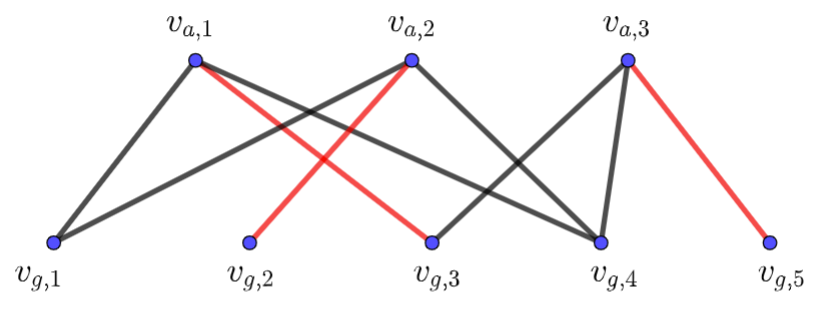
|
| (b) Auxiliary bipartite graph |
In the Gallai-Edmonds decomposition and a maximum matching of a general graph , as Figure 8 illustrates, the isolated -exposed vertex in cannot access to that in by any alternating paths. It can be shown that Hall’s condition holds for any [15, 16], thus the restricts to a matching on bipartite graph that covers .
Since each odd component is factor-critical, and any vertex of can be the one unmatched by a maximum matching . Thus, the only unmatched vertex in each odd component can either be matched with a vertex , or be isolated in the odd component . Therefore, any free vertex can only be the source of an augmenting path at most once in the DFS algorithm. Since the initial number of free vertices is upper bounded by the order of , and the length of each alternating path is proportional to the number of edges , the complexity of the DFS algorithm is given in Theorem 3.
Theorem 3.
The DFS algorithm can determine a maximum matching of a general graph in time with space complexity .
Experiments were conducted to verify the performance of our maximum matching algorithm. A set of -regular graphs with vertices and edges was randomly generated. Figure 9 shows the experimental results of average running time, in which 25 graphs were randomly generated for every pair of , and . These experimental results confirm the performance of our maximum matching algorithm given in Theorem 3. As shown in Figure 9, for each set of graphs under consideration, the running time of our algorithm is on the order of for a given degree .

5 Conclusion
The fundamental problem of finding maximum matchings in general graphs is the existence of odd cycles, or blossoms. Instead of shrinking blossoms, this paper proposed a deflection algorithm to cope with the parity conflicts caused by odd cycles. This new algorithm achieves time complexity with space complexity. This newly proposed algorithm is complementary to Edmonds’ blossom algorithm in two important aspects: depth-first search (DFS) versus breadth-first search (BFS), and deflection from blossoms versus shrinking of blossoms. In the future, we will explore the application of this method to maximum matching of weighted graphs.
ACKNOWLEDGMENTS
The authors would like to thank Professor Shahbaz Khan of Department of Computer Science and Engineering, Indian Institute of Technology, Roorkee, India, for many useful criticism and suggestions.
References
- [1] L. Lovász and M. D. Plummer, Matching theory, vol. 367. American Mathematical Society, 2009.
- [2] T. H. Cormen, C. E. Leiserson, R. L. Rivest, and C. Stein, Introduction to algorithms. MIT press, 2009.
- [3] J. E. Hopcroft and R. M. Karp, “An algorithm for maximum matchings in bipartite graphs,” SIAM Journal on Computing, vol. 2, no. 4, pp. 225–231, 1973.
- [4] J. Edmonds, “Paths, trees, and flowers,” Canadian Journal of Mathematics, vol. 17, pp. 449–467, 1965.
- [5] H. N. Gabow, “An efficient implementation of Edmonds’ algorithm for maximum matching on graphs,” Journal of the ACM (JACM), vol. 23, no. 2, pp. 221–234, 1976.
- [6] H. N. Gabow and R. E. Tarjan, “A linear-time algorithm for a special case of disjoint set union,” Journal of Computer and System Sciences, vol. 30, no. 2, pp. 209–221, 1985.
- [7] S. Micali and V. V. Vazirani, “An algorithm for finding maximum matching in general graphs,” in 21st Annual Symposium on Foundations of Computer Science (1980), pp. 17–27, IEEE, 1980.
- [8] V. V. Vazirani, “A theory of alternating paths and blossoms for proving correctness of the general graph maximum matching algorithm,” Combinatorica, vol. 14, no. 1, pp. 71–109, 1994.
- [9] R. E. Tarjan, Data structures and network algorithms. SIAM, 1983.
- [10] C. Berge, “Two theorems in graph theory,” Proceedings of the National Academy of Sciences of the United States of America, vol. 43, no. 9, pp. 842–844, 1957.
- [11] T. T. Lee, Y. Wan, and H. Guan, “Randomized -edge colouring via exchanges of complex colours,” International Journal of Computer Mathematics, vol. 90, no. 2, pp. 228–245, 2013.
- [12] L. Wang, T. Ye, T. T. Lee, and W. Hu, “A parallel complex coloring algorithm for scheduling of input-queued switches,” IEEE Transactions on Parallel and Distributed Systems, vol. 29, no. 7, pp. 1456–1468, 2018.
- [13] T. Gallai, “Kritische graphen ii,” Magyar Tud. Akad. Mat. Kutato Int. Kozl., vol. 8, pp. 373–395, 1963.
- [14] L. Lovász and M. D. Plummer, Matching Theory, vol. 29. Annals of Discrete Mathematics, North-Holland, Amsterdam, 1986.
- [15] D. B. West, “A short proof of the Berge–Tutte formula and the Gallai–Edmonds structure theorem,” European Journal of Combinatorics, vol. 32, no. 5, pp. 674–676, 2011.
- [16] D. B. West, Introduction to graph theory. Prentice-Hall, Inc., Upper Saddle River, 2001.