Smooth Hybrid Inflation with Low Reheat Temperature and Observable Gravity Waves

Among the various proposed models of cosmic inflation, supersymmetric hybrid inflation models [1, 2, 3, 4, 5] have gained immense attention. They provide compelling framework to realize inflation within the grand unified theories (GUTs) of particle physics. Several GUTs such as $SU(5)$ [6], Flipped $SU(5)$ [7, 8] and the Pati-Salam symmetry $SU(4)_{C}\times SU(2)_{L}\times SU(2)_{R}$ [9, 10] and its supersymmetric variants  [11] have been employed successfully to realize hybrid inflation [12, 13]. In this work, we implement the hybrid inflation scenario in the $SU(5)$ GUT model extended by a $U(1)_{\chi}$ symmetry [14]. The $U(1)_{\chi}$ charge assignment is such that the whole gauge group of the model is embedded in $SO(10)$, i.e., $SU(5)\times U(1)_{\chi}\in SO(10)$. This model is worth exploring due to its various attractive features which are not present in the stardard $SU(5)$ [6]. For example, in the $SU(5)$ model, a discrete $Z_{2}$ symmetry is imposed by hand to avoid rapid proton decay whereas, in $SU(5)\times U(1)_{\chi}$ this $Z_{2}$ symmetry -inherited from $SO(10)$ [15] - is encoded into $U(1)_{\chi}$ and arises naturally after the spontaneous breaking of this abelian factor. This $Z_{2}$ symmetry induces two welcome properties. First it serves as the matter parity of the Minimal Supersymmetric Standard Model (MSSM) and secondly it ensures the existence of a stable lightest supersymmetric particle (LSP) which can be a viable cold dark matter candidate. Furthermore, the right-handed neutrino mass in $SU(5)$ model obtained by including the singlet right-handed neutrinos is inadequate since there is no symmetry preventing the neutrino mass to become arbitrarily large. In $SU(5)\times U(1)_{\chi}$ model however, the right-handed neutrino mass is generated by the breaking of $U(1)_{\chi}$ symmetry after one of the fields carrying $U(1)_{\chi}$ charge acquires a Vacuum Expectation Value (VEV) at an appropriately high scale. Hence, $SU(5)\times U(1)_{\chi}$ retains many interesting features of the $SO(10)$ covering GUT while it relaxes some severe constraints emanating from the $SO(10)$ unification. Furthermore, there are additional constraints on the Higgs spectrum in  $SO(10)$ inflationary scenarios [18, 19] stemming from the fact that large Higgs representations (such as the $\underline{126}$ of $SO(10)$ ) induce large contributions to the beta-functions so that the Renormalization Group evolution drives the gauge couplings to the non-perturbative regime [20]. On the contrary, we will see for example that certain $SU(5)\times U(1)$ components of the $\underline{126}$ representation play an essential rôle, and can be incorporated in the spectrum without spoiling the perturbative unification. We note in passing that in string derived constructions there are alternative mechanisms, such as fluxes and Wilson lines breaking GUTs such as the $SO(10)$, and the $SU(5)\times U(1)_{\chi}$ follows naturally as an effective field theory model [21].

In this paper, we consider smooth hybrid inflation in the supersymmetric $SU(5)\times U(1)_{\chi}$ with $SU(5)\times U(1)_{\chi}$ symmetry broken during inflation, inflating both the monopoles and cosmic strings away. Note that in smooth hybrid inflation, the scalar spectral index $n_{\rm s}$ lies in the observed range of Planck [22] provided the inflationary potential incorporates either the soft supersymmetry (SUSY) breaking terms, or higher-order terms in the Kähler potential [23, 24]. Without these terms, the scalar spectral index $n_{\rm s}$ lies close to 0.98 which is acceptable only if the effective number of light neutrino species are slightly greater than 3 [25].

It has been observed (see for example [26, 27, 28]), that a red tilted scalar spectral index ($n_{s}<1$), consistent with the Planck bounds cannot be achieved with the minimal Kähler potential. In the present work we show for the first time that, by taking soft SUSY contribution into account along with the supergravity (SUGRA) corrections in a minimal Kähler potential setup, the predictions of smooth hybrid inflation model are consistent with the Planck’s latest bounds on scalar spectral index $n_{s}$. We also obtain a low reheat temperature $T_{r}\simeq 10^{6}$ GeV, although the tensor to scalar ratio $r$ remains extremely small. However, the value of gravitino mass $m_{3/2}$ required to avoid $d=5$ proton decay cannot be achieved. Remarkably, by employing a non-minimal Kähler potential, successful inflation is realized with the central value of Planck’s bound on $n_{s}$ and large tensor-to-scalar ratio $r$, see Ref [29]. Moreover, the dangerous $d=5$ rapid proton decay, mediated by color-triplet Higgsinos [30], is avoided for split [31] and high scale SUSY [32]. The proton lifetime for the decay $p\rightarrow K^{+}\bar{\nu}$ satisfies the current Super-Kamiokande [33] experimental bounds for the range of $SU(5)$ symmetry breaking scale $M$ and gravitino mass $m_{3/2}$, obtained in this model. We have also include the future expected sensitivity (in the absence of any proton-decay signal) of the Hyper-Kamiokande experiment [34]. The non-thermal leptogenesis yields a low reheat temperature $(3\times 10^{6}\lesssim T_{r}\lesssim 7\times 10^{7})$ GeV, avoiding the gravitino problem [35] ⁵⁵ 5 For additional references on this issue see for example [36]. for the full range of gravitino masses. These results can be improved by using the exact calculation for $d=5$ proton decay lifetime, which may reduce the SUSY breaking scale ($M_{SUSY}$) avoiding the $d=5$ proton decay in the minimal Kähler potential setup as well.

The future experiments will considerably improve the measurements of the tensor-to-scalar ratio $r$, a canonical measure of primordial gravity waves. One of the highlights of PRISM [37] is to detect inflationary gravity waves with $r$ as low as $5\times 10^{-4}$, and an important goal of LiteBIRD [38] is to attain a measurement of $r$ within an uncertainty of $\delta r=10^{-3}$. Future missions include PIXIE [39], which aims to measure $r<10^{-3}$ at five standard deviations, and CORE [40], which forecasts to lower the detection limit for the tensor-to-scalar ratio down to the $10^{-3}$ level. A low reheat temperature with observable primordial gravity waves is a particular feature of the model under consideration. We obtain a tensor to scalar ratio $r$ as large as $\sim 10^{-2}$ which is measurable by current and future experiments.

The rest of the paper is organised as follows. In section 2 we describe the basic features of the $SU(5)\times U(1)_{\chi}$ model including the superfields, their charge assignments, the superpotential terms constrained by a $U(1)_{R}$ symmetry, and proton decay constraints. In section 3 we discuss smooth hybrid inflation while reheating and non-thermal leptogenesis discussed in section 4. We present the numerical results with minimal Kähler potential in section 5 and non-minimal Kähler potential in section 6. Finally we summarize the results in section 7.

In this section we present the key features of the effective $SU(5)\times U(1)_{\chi}$ model which are essential for the description of the inflationary scenario to be implemented subsequently. We mainly focus on the massless spectrum and the properties with respect to the symmetry breaking pattern.

The MSSM matter superfields reside in the $10$, $\bar{5}$ and $1$ dimensional representations of the group $SU(5)$ and constitute the $\underline{16}$ (spinorial) representation of $SO(10)$. Their decomposition with respect to the $SU(3)\times SU(2)_{L}\times U(1)_{Y}$ gauge symmetry is

$$\begin{split}F_{i}&\equiv 10_{-1}=Q(3,2)_{\frac{1}{6}}+u^{c}(\overline{3},1)_{-\frac{2}{3}}+e^{c}(1,1)_{1}~,\\ \bar{f}_{i}&\equiv\bar{5}_{+3}=d^{c}(\bar{3},1)_{\frac{1}{3}}+\ell(1,2)_{-\frac{1}{2}}~,\\ \nu_{i}^{c}&\equiv 1_{-5}=\nu^{c}(1,1)_{0}~,\end{split}$$

(1)

where $i=1,2,3$ is the generation index. The indices on the left hand side of the above decomposition denote the $U(1)_{\chi}$ charges (in units of $2/\sqrt{10}$) of $10,\bar{5},1$ representations, whilst on the right hand side they stand for the hypercharge assignments. Furthermore, the singlet $1_{-5}$ is identified with the right-handed neutrino superfield $\nu^{c}$.

The charge assignments listed in Table 1 may suggest that the non zero VEVs of $\chi$, $\bar{\chi}$ (carrying $U(1)_{\chi}$ charges $10$ and $-10$ respectively) break $U(1)_{\chi}$ to $Z_{10}$. However, since the $Z_{5}$ subgroup of $Z_{10}$ also resides in $SU(5)$, the effective unbroken discrete symmetry is $Z_{2}$ [14, 15]. In $SO(10)$ representations, the $Z_{2}$ symmetry is manifested as $D$-parity, i.e., the discrete $SO(10)$ element[16, 15] which transforms left handed fields to their right-handed conjugates. Since the matter fields contain only fields of a single chirality, there can be no well-defined notion of parity in $SO(10)$. $D$-parity then plays a role to create the possibility for the presence of $C$ and $P$ at lower energies and acts as MSSM matter parity, see Ref [16, 17]. Moreover, the $Z_{2}$ symmetry and the particular field assignment with standard matter parity is justified by the $SO(10)$ embedding of the present model. This can be seen by noticing that the content of each fermion generation (including the right-handed neutrino) is embedded in the fundamental 16-spinorial representation of $SO(10)$ (hence, as it was observed in [15] the actual symmetry is its simply-connected spin(10)) and the Higgs in 10 representation of $SO(10)$. The successive breaking with the $126_{H}$ (which includes the singlet $\chi$) and $10_{H}$ (which contains the SM Higgs), defines a $Z_{2}$ matter parity which remains unbroken by the subsequent symmetry breaking to SM group.

In the following we implement the $R$-charge assignment (as shown in Table 1) of the superfields proposed in [41]. In addition, imposing a $Z_{3}$ symmetry on the Higgs superfield $\Phi$ under which, $\Phi\rightarrow e^{2\dot{\iota}\pi/3}\Phi$ (with other fields trasforming trivially), only cubic powers of $\Phi$ are allowed in the superpotential. The complete spectrum of the model with its various transformation properties are shown in Table 1. The $SU(5)\times U(1)_{\chi}$, $U(1)_{R}$, and $Z_{3}$ symmetric superpotential of the model with the leading-order non-renormalizable terms is given by ⁶⁶ 6 For smooth SU(5) hybrid inflation, see ref. [28].

	$\displaystyle W$	$\displaystyle=$	$\displaystyle S\left(\mu^{2}+\frac{Tr(\Phi^{3})}{m_{P}}\right)+\gamma\frac{\bar{h}\Phi^{3}h}{m_{P}^{2}}+\delta\bar{h}h+\sigma_{\chi}S\left(\chi\bar{\chi}-\mu_{\chi}^{2}\right)$		(3)
		$\displaystyle+$	$\displaystyle y_{ij}^{(u)}\,F_{i}\,F_{j}\,h+y_{ij}^{(d,e)}\,F_{i}\,\bar{f}_{j}\,\bar{h}+y_{ij}^{(\nu)}\,\nu_{i}^{c}\,\bar{f}_{j}\,h+\zeta_{ij}\chi\nu_{i}^{c}\nu_{j}^{c},$

where $\mu$ is a superheavy mass and $m_{P}=2.43\times 10^{18}$ GeV is the reduced Planck mass. The Yukawa couplings $y_{ij}^{(u)}$, $y_{ij}^{(d,e)}$, $y_{ij}^{(\nu)}$ in the second line of (3) generate Dirac masses for quarks and leptons after the electroweak symmetry breaking, whereas $m_{\nu_{ij}}=\zeta_{ij}\mu_{\chi}$ is the right-handed neutrino mass matrix, generated after $\chi$ acquires a VEV, $\langle\chi\rangle=\mu_{\chi}$, breaking the $U(1)_{\chi}$ factor.

A few comments regarding the merits of the additional symmetries are worth mentioning. By virtue of the global $U(1)_{R}$ symmetry the superpotential $W$ exhibits a number of interesting features. First, we observe that only linear terms in $S$ are allowed in $W$ whereas higher order ones, such as $S^{2}$, are prevented. This is a welcome fact since $S^{2}$-terms could generate an inflaton mass of Hubble size, $H\simeq\sqrt{V(x)/3m_{P}^{2}}$, invalidating the inflationary scenario. Furthermore, under the action of the $U(1)_{R}$ symmetry the model naturally avoids the $\eta$ problem [3], that appears when SUGRA corrections are included. Finally, due $U(1)_{R}$ several dangerous dimension-5 proton decay operators are suppressesed. The $Z_{3}$ symmetry plays an important rôle in realizing smooth hybrid inflation. At this point it should be emphasized that in the absence of this symmetry, the above superpotential (3) reduces to the superpotential of shifted hybrid inflation model [41]. As compared to this latter one, the smooth hybrid inflation proposed in the present work generally predicts large tensor modes.

Next, we discuss in brief the implementation of the douplet-triplet solution to the well known issue of the color triplets $D_{h},\bar{D}_{\bar{h}}$ embedded in the same representations $5$ and $\bar{5}$ with the MSSM Higgs fields. The relevant superpotential terms are

$$W\supset\gamma\frac{\bar{h}\Phi^{3}h}{m_{P}^{2}}+\delta\bar{h}h~.$$

(4)

After the symmetry breaking, these can be written in terms of the MSSM fields as follows

$$W\supset\left(\delta-\frac{9\gamma}{40\sqrt{15}}\frac{M^{3}}{m_{P}^{2}}\right)h_{u}h_{d}+\left(\delta+\frac{\gamma}{15\sqrt{15}}\frac{M^{3}}{m_{P}^{2}}\right)\bar{D}_{\bar{h}}D_{h}\supset\mu h_{u}h_{d}+M_{D_{h}}\bar{D}_{\bar{h}}D_{h}~.$$

(5)

We observe that the doublet-triplet splitting problem is effectuated by requiring fine-tuning of the involved parameters, such that

$$\delta\sim\frac{9\gamma}{40\sqrt{15}}\frac{M^{3}}{m_{P}^{2}}~.$$

Here $\mu$ is the MSSM $\mu$ parameter taken to be of the order of TeV scale while, $M_{D_{h}}$ is the color triplet Higgs mass parameter given by,

$$M_{D_{h}}\sim\frac{7\,\gamma}{24\sqrt{15}}\frac{M^{3}}{m_{P}^{2}}.$$

(6)

The dominant contribution to proton decay amplitude comes from color-triplet Higgsinos. The decay rate from dimension 5 operator mediated by color-triplet Higgsinos typically dominates the decay rate from gauge boson mediated dimension 6 operators. The proton lifetime for the decay $p\rightarrow K^{+}\bar{\nu}$ mediated by color-triplet Higgsinos is approximated by the following formula [42]:

$$\tau_{p}\simeq 4\times 10^{35}\times\sin^{4}2\beta\left(\frac{M_{\text{SUSY}}}{10^{2}~\text{TeV}}\right)^{2}\left(\frac{M_{D_{h}}}{10^{16}~\text{GeV}}\right)^{2}\text{yrs}.$$

(7)

The proton lifetime depends on Higgino mass as well as the SUSY breaking scale $M_{SUSY}$. The experimental bounds on the proton lifetime can be satisfied at High scale SUSY.

Figure 1 shows $SU(5)$ gauge symmetry breaking scale $M$ as a function of SUSY breaking scale $M_{SUSY}$. The curves represent different values of $\tan\beta$. The left panel is drawn for proton lifetime fixed at current Super-Kamiokande bounds [33] whilst the right panel is drawn for the future expected proton lifetime sensitivity limit⁷⁷ 7 We emphasize that here we consider the Hyper-Kamiokande future expected limits in the case of non-observation of proton decay signals in order to show the status of proton decay in our model from future prospective. of Hyper-Kamiokande experiment [34]. If the split and high scale SUSY is implemented, proton decay rate is within the acceptable bounds. The range of $M$ obtained in our numerical results in section 5 is consistent with the experimental bounds on proton lifetime.

We will compute the effective scalar potential considering contributions from the F- and D-term sectors. The superpotential terms relevant for inflation are

$\displaystyle W$

$\displaystyle\supset$

$\displaystyle S\left(\mu^{2}+\frac{Tr(\Phi^{3})}{m_{P}}\right)+\gamma\frac{\bar{h}\Phi^{3}h}{m_{P}^{2}}+\delta\bar{h}h+\sigma_{\chi}S\left(\chi\bar{\chi}-\mu_{\chi}^{2}\right)+\zeta_{ij}{\chi}\nu_{i}^{c}\nu_{j}^{c}~.$

(8)

In component form, the above superpotential is expanded as follows,

	$\displaystyle W\supset S\left(\mu^{2}+\frac{1}{4m_{P}}d_{ijk}\phi_{i}\phi_{j}\phi_{k}\right)$	$\displaystyle+$	$\displaystyle\delta\bar{h}_{a}h_{a}+\gamma\frac{\bar{h}_{a}h_{d}}{m_{P}^{2}}T^{i}_{ab}T^{j}_{bc}T^{k}_{cd}\,\phi_{i}\phi_{j}\phi_{k}$		(9)
		$\displaystyle+$	$\displaystyle\sigma_{\chi}S\left(\chi\bar{\chi}-\mu_{\chi}^{2}\right)+\zeta_{ij}{\chi}\nu_{i}^{c}\nu_{j}^{c},$

where $\Phi=\phi_{i}T^{i}$ with Tr$[T_{i}T_{j}]=\frac{1}{2}\delta_{ij}$ and $d_{ijk}=2$Tr$[T_{i}\{T_{j},T_{k}\}]$ in the $SU(5)$ adjoint basis. The $F$-term scalar potential obtained from the above superpotential is given by

	$\displaystyle V_{F}$	$\displaystyle=$	$\displaystyle\left|\;\mu^{2}+\frac{1}{4m_{P}}d_{ijk}\phi_{i}\phi_{j}\phi_{k}+\sigma_{\chi}\left(\chi\bar{\chi}-\mu_{\chi}^{2}\right)\;\right|^{2}$		(10)
		$\displaystyle+$	$\displaystyle\sum_{i}\left|\;\frac{3}{4m_{P}}d_{ijk}S\phi_{j}\phi_{k}+3\,\gamma\frac{\bar{h}_{a}h_{d}}{m_{P}^{2}}T^{i}_{ab}T^{j}_{bc}T^{k}_{cd}\,\phi_{j}\phi_{k}\;\right|^{2}$
		$\displaystyle+$	$\displaystyle\sum_{d}\left|\delta\bar{h_{d}}+\gamma\frac{\bar{h}_{a}}{m_{P}^{2}}T^{i}_{ab}T^{j}_{bc}T^{k}_{cd}\,\phi_{i}\phi_{j}\phi_{k}\right|^{2}+\sum_{d}\left|\delta h_{d}+\gamma\frac{h_{a}}{m_{P}^{2}}T^{i}_{ab}T^{j}_{bc}T^{k}_{cd}\,\phi_{i}\phi_{j}\phi_{k}\right|^{2}$
		$\displaystyle+$	$\displaystyle\left|\,\sigma_{\chi}S\bar{\chi}+\zeta_{ij}\nu_{i}^{c}\nu_{j}^{c}\,\right|^{2}+\left|\,\sigma_{\chi}S\chi\,\right|^{2}+\left|2\zeta_{ij}{\chi}\nu_{i}^{c}\right|^{2},$

where the scalar components of the superfields are denoted by the same symbols as the corresponding superfields. The VEV’s of the fields at the global SUSY minimum of the above potential are given by,

	$$\displaystyle S^{0}=h_{a}^{0}=\bar{h_{a}^{0}}=\nu_{i}^{c\,0}=0,$$
	$$\displaystyle\;\;\chi^{0}=\bar{\chi}^{0}=\mu_{\chi},\;\;Tr[(\Phi^{0})^{3}]=d_{ijk}\phi_{i}^{0}\phi_{j}^{0}\phi_{k}^{0}=-M^{3}/\sqrt{15},$$		(11)

where

$\displaystyle M=\left[4\sqrt{15}\,m_{P}\,\mu^{2}\right]^{1/3}.$

(12)

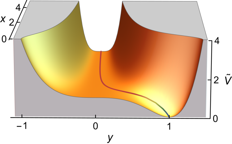
The superscript ‘0’ denotes the field value at its global minimum. The superfield pair $\chi,\bar{\chi}$ which is $SU(5)$ singlet acquires an intermediate scale VEV such that $U(1)_{\chi}$ breaks to $Z_{2}$, the matter parity. This symmetry ensures the existence of a lightest supersymmetric particle (LSP) which could play the rôle of a cold dark matter component. Further, as discussed in [14], this $Z_{2}$ symmetry yields topologically stable cosmic strings. Using $SU(5)$ symmetry transformation the VEV matrix $\Phi^{0}=\phi_{i}^{0}T^{i}$ can be aligned in the $24$-direction,

$$\Phi_{24}^{0}=\frac{\phi_{24}^{0}}{\sqrt{15}}\left(1,1,1,-3/2,-3/2\right).$$

(13)

This implies that $\phi_{i}^{0}=0,\,\forall\,i\neq 24$ and $\phi_{24}^{0}=M$, where $d_{24\,24\,24}=-1/\sqrt{15}$ and $\phi_{i}^{0*}=\phi_{i}^{0}$ have been assumed. Thus the $SU(5)$ gauge symmetry is broken down to Standard Model gauge group $G_{\text{SM}}$ by the non-vanishing VEV of $\phi_{24}^{0}$ which is a singlet under $G_{\text{SM}}$.

The $D$-term scalar potential,

	$\displaystyle V_{D}$	$\displaystyle=$	$\displaystyle\frac{g_{5}^{2}}{2}\sum_{i}\left(f^{ijk}\phi_{j}\phi_{k}^{\dagger}+T^{i}\left(\left|h_{a}\right|^{2}-\left|\bar{h}_{a}\right|^{2}\right)\right)^{2}$		(14)
		$\displaystyle+$	$\displaystyle\frac{g_{\chi}^{2}}{2}\left(q_{\chi}\left|\chi\right|^{2}+q_{\bar{\chi}}\left|\bar{\chi}\right|^{2}+\left(q_{\bar{\chi}}+q_{\chi}\right)\varsigma\right)^{2},$

also vanishes for this choice of the VEV (since $f^{i,24,24}=0$) and for $|\bar{h}_{a}|=|h_{a}|$, $|\bar{\chi}|=|\chi|$. Here the symbol $\varsigma$ stands for the Fayet-Iliopoulos coupling constant.

The scalar potential in Eq. (10) can be written in terms of the dimensionless variables

$$x=\frac{|S|}{M}~,~~~~~~~~~~~~y=\frac{\phi_{24}}{M}~,~~~~~~~~~~~z=\frac{\chi}{M}~,$$

(15)

as follows,

$$V=\mu^{4}\left(\left(1-y^{3}+\frac{\sigma_{\chi}}{\mu^{2}}\left(M^{2}z^{2}-\mu_{\chi}^{2}\right)\right)^{2}+9x^{2}y^{4}\right)+2\sigma_{\chi}^{2}M^{4}z^{2}x^{2}~.$$

(16)

Because the potential (10) is a complicated function of the fields $\phi_{24}$, $S$, $\chi$, $\bar{\chi}$, in order to make the computation of the extrema tractable, we have assumed $\chi=\bar{\chi}=\mu_{\chi}$, in accordance with their VEVs at the global SUSY minimum. We have checked with specific numerical examples that this simplification preserves the main features of the inflationary analysis in the parameter region of our interest. Indeed, this is due to the fact that in the present model, the $U(1)_{\chi}$ symmetry is broken after the $SU(5)$ symmetry so that the breaking scale $M$ of $SU(5)$ is always higher than the breaking scale $\mu_{\chi}$ of $U(1)_{\chi}$ which does not affect the inflation trajectory. Therefore, the potential can safely be stabilized at $z=\mu_{\chi}/M$. It can readily be checked that for $\mu_{\chi}\leq M$, the inflationary trajectories, in particular, remain unaltered in the $y-x$ plane. For $\mu_{\chi}>M$ however, the inflationary trajectory is affected and the potential is lifted. The potential is displayed in Fig. (2) which shows a valley of minimum given by

$$y=\frac{1}{{2}^{1/3}}\left(({\sqrt{32x^{6}+1}+1})^{1/3}-({\sqrt{32x^{6}+1}-1})^{1/3}\right)$$

(17)

which in the large $x$ limit can be approximated as $y\approx\frac{1}{6\,x^{2}}.$

This valley of local minimum is not flat and possess a slope to drive inflaton towards SUSY vacuum. Here we assume special initial conditions for inflation to occur in the valley ⁸⁸ 8 See however [43] references therein for a detailed discussion of the fine-tuning of initial conditions in various models of SUSY hybrid inflation.. Implementing the large $x$ behaviour ($x\gg 1$) during inflation the global SUSY potential (16) takes the form,

$$V\simeq\mu^{4}\left(1-\frac{1}{432\,x^{6}}\right)+2\,\mu_{\chi}^{2}\sigma_{\chi}^{2}M^{2}x^{2}.$$

(18)

As soon as the inflation epoch ends, the vacuum energy is transfered to the energies of coherent oscillations of the inflaton $S$ and the scalar field $\theta=(\chi+\bar{\chi})/\sqrt{2}$ whose decays give rise to the radiation in the universe. Reheating with leptogenesis, requires the presence of lepton-number violating interactions with the inflaton which decays into right-handed neutrinos. The latter are involved in the following superpotential terms

$$W\supset\sigma_{\chi}S\chi\bar{\chi}+\zeta_{ij}\chi\nu_{i}^{c}\nu_{j}^{c}+\overline{\zeta_{ij}}\frac{\chi\chi}{\Lambda}\nu_{i}^{c}\nu_{j}^{c},$$

(19)

where $\overline{\zeta_{ij}}$ is a coupling constant and $\Lambda$ represents a high cut-off scale (in a string model this could be identified with the compactification scale). Heavy Majorana masses for the right-handed neutrinos are provided by the two last terms of (19)

$$M_{\nu^{c}_{ij}}=\zeta_{ij}\langle\chi\rangle+\overline{\zeta_{ij}}\frac{\langle\chi\rangle\langle\chi\rangle}{\Lambda}~\cdot$$

(20)

Also, Dirac neutrino masses of the order of the electroweak scale are obtained from the tree-level superpotential term $y_{ij}^{(\nu)}\,\nu_{i}^{c}\,\bar{f}_{j}\,h\to m_{ij}^{\nu_{D}}\nu\nu^{c}$ given in (3). Thus, the neutrino sector is

$$W\supset{m_{\nu_{D}}}_{ij}\nu_{i}\nu_{j}^{c}+M_{\nu^{c}_{ij}}\nu_{i}^{c}\nu_{j}^{c}.$$

(21)

Note that the last term in (21) violates lepton number by two units, $\Delta L=2$. The small neutrino masses supported by neutrino oscillation experiments, are obtained by integrating out the heavy right-handed neutrinos and read as

$${m_{\nu_{D}}}_{\alpha\beta}=-\sum_{i}{y^{(\nu)}}_{i\alpha}{y^{(\nu)}}_{i\beta}\frac{v_{u}^{2}}{M_{i}}~\cdot$$

(22)

The neutrino mass matrix ${m_{\nu_{D}}}_{\alpha\beta}$ can be diagonalized by a unitary matrix $U_{\alpha i}$ as ${m_{\nu_{D}}}_{\alpha\beta}=U_{\alpha i}U_{\beta i}m_{\nu_{D}}$, where $m_{\nu_{D}}$ is a diagonal mass matrix $m_{\nu_{D}}={\rm diag}(m_{\nu_{1}},m_{\nu_{2}},m_{\nu_{3}})$ and $M_{i}$ represent the eigenvalue of mass matrix $M_{\nu^{c}_{ij}}$.

Another important implication of $\Delta L=2$ term is that lepton asymmetry is generated (inducing also baryon asymmetry [44, 45]) through right-handed neutrino decays, due to one-loop self-energy (CP-violating) diagrams. There are contributions to two different decay channels and the ratio of the lepton number density to the entropy density in the limit $T_{r}<M_{1}\leq m_{\text{inf}}/2\leq M_{2,3}$ is defined as

$$\frac{n_{L}}{s}\sim\frac{3}{2}\frac{T_{r}}{m_{\text{inf}}}\epsilon_{cp}~,$$

(23)

where $\epsilon_{cp}$ is the CP asymmetry factor and is generated from the out of equilibrium decay of lightest right-handed neutrino and is given by [46],

$$\epsilon_{cp}=-\frac{3}{8\pi}\frac{1}{\left(y^{(\nu)}y^{{(\nu)}\dagger}\right)_{11}}\sum_{i=2,3}Im\left[\left(y^{(\nu)}y^{{(\nu)}\dagger}\right)_{1i}\right]^{2}\frac{M_{1}}{M_{i}},$$

(24)

and $T_{r}$ is reheating temperature which can be as estimated as

$\displaystyle T_{r}\simeq\sqrt[4]{\frac{90}{\pi^{2}g_{\star}}}\sqrt{\Gamma\,m_{P}}~,$

(25)

where $g_{\star}$ is $228.75$ for MSSM. The $\Gamma$ is the decay width for the inflaton decay into right-handed neutrinos and is given by [46]

$$\Gamma\left({\rm inf}\rightarrow\nu_{i}^{c}\nu_{j}^{c}\right)=\frac{1}{8\pi}\left(\frac{M_{1}}{\mu_{\chi}}\right)^{2}\,m_{\text{inf}}\left(1-\frac{4M_{1}^{2}}{m_{\text{inf}}^{2}}\right)^{1/2},$$

(26)

with the inflaton mass given by

$$m_{\text{inf}}=\sqrt{\frac{9\mu^{4}}{M^{2}}+2\mu_{\chi}^{2}\sigma_{\chi}^{2}}\,\,.$$

(27)

Assuming a normal hierarchical pattern of light neutrino masses, the CP asymmetry factor, $\epsilon_{cp}$, becomes

$$\epsilon_{cp}=\frac{3}{8\pi}\frac{M_{1}m_{\nu_{3}}}{v_{u}^{2}}\delta_{\rm eff},$$

(28)

where $m_{\nu_{3}}$ is the mass of the heaviest light neutrino, $v_{u}=\langle H_{u}\rangle$ is the VEV of the up-type electroweak Higgs and $\delta_{\rm eff}$ is the CP-violating phase. The experimental value of lepton asymmetry is estimated as [47],

$\displaystyle\mid n_{L}/s\mid\approx\left(2.67-3.02\right)\times 10^{-10}.$

(29)

In the numerical estimates discussed below we take $m_{\nu_{3}}=0.05$ eV, $|\delta_{\rm eff}|=1$ and $v_{u}=174$ GeV, while assuming large $\tan\beta$. The non-thermal production of lepton asymmetry, $n_{L}/s$, is given by the following expression

$$\frac{n_{L}}{s}\lesssim 3\times 10^{-10}\frac{T_{r}}{m_{\text{inf}}}\left(\frac{M_{1}}{10^{6}\text{ GeV}}\right)\left(\frac{m_{\nu_{3}}}{0.05\text{ eV}}\right),$$

(30)

with $M_{1}\gg T_{r}$. Using the experimental value of $n_{L}/s\approx 2.5\times 10^{-10}$ with Eq. (25) and (30), we obtain the following lower bound on $T_{r}$,

$$T_{r}\gtrsim 1.9\times 10^{7}\text{ GeV}\left(\frac{m_{\text{inf}}}{10^{11}\text{ GeV}}\right)^{3/4}\left(\frac{10^{16}\,\text{GeV}}{M_{1}}\right)^{1/2}\left(\frac{m_{\nu_{3}}}{0.05\text{ eV}}\right)^{1/2}.$$

(31)

A successful baryogenesis is usually generated through the sphaleron processe where an initial lepton asymmetry, $n_{L}/s$, is partially converted into a baryon asymmetry $n_{B}/s=-0.35n_{L}/s$ [48, 49]. Eq. (31) is used in our numerical analysis to calculate inflationary predictions which are consistent with leptogenesis and baryogenesis.

In this section we will include SUGRA corrections in the effective potential and consider their implications in the inflationary parameters. We first start with the minimal canonical Kähler potential,

$$K=|S|^{2}+Tr|\Phi|^{2}+|h|^{2}+|\bar{h}|^{2}+|\chi|^{2}+|\bar{\chi}|^{2}.$$

(32)

The F-term SUGRA scalar potential is given by

$$V_{\text{SUGRA}}=e^{K/m_{P}^{2}}\left(K_{i\bar{j}}^{-1}D_{z_{i}}WD_{z^{*}_{j}}W^{*}-3m_{P}^{-2}\left|W\right|^{2}\right),$$

(33)

with $z_{i}$ being the bosonic components of the superfields $z_{i}\in\{S,\Phi,h,\bar{h},\chi,\bar{\chi},\cdots\}$, and we have defined

$$D_{z_{i}}W\equiv\frac{\partial W}{\partial z_{i}}+m_{P}^{-2}\frac{\partial K}{\partial z_{i}}W,\,\,\,K_{i\bar{j}}\equiv\frac{\partial^{2}K}{\partial z_{i}\partial z_{j}^{*}},$$

(34)

and $D_{z_{i}^{*}}W^{*}=\left(D_{z_{i}}W\right)^{*}.$ The SUGRA scalar potential during inflation becomes

	$\displaystyle V_{\text{SUGRA}}$	$\displaystyle=$	$\displaystyle\mu^{4}\,\left[1-\frac{1}{432\,x^{6}}+2\,\left(\frac{\mu_{\chi}}{m_{P}}\right)^{2}+2\,\left(\frac{\mu_{\chi}}{m_{P}}\right)^{4}+\frac{40}{3}\sigma_{\chi}^{2}\left(\frac{\mu_{\chi}}{m_{P}}\right)^{2}\right.$		(35)
		$\displaystyle+$	$\displaystyle\left.2\,x^{2}\left(\frac{M}{m_{P}}\right)^{2}\left(\frac{\mu_{\chi}}{m_{P}}\right)^{2}+\frac{x^{4}}{2}\left(\frac{M}{m_{P}}\right)^{4}\right]+2\,M^{4}x^{4}\left[\left(\frac{\mu_{\chi}}{m_{P}}\right)^{2}+2\left(\frac{\mu_{\chi}}{m_{P}}\right)^{4}\right]\sigma_{\chi}^{2}$
		$\displaystyle+$	$\displaystyle 4\,\mu^{2}\sigma_{\chi}\,\left[x^{4}\,\mu_{\chi}^{2}\left(\frac{M}{m_{P}}\right)^{4}+x^{2}M^{2}\left(\left(\frac{\mu_{\chi}}{m_{P}}\right)^{2}+2\,\left(\frac{\mu_{\chi}}{m_{P}}\right)^{4}\right)\right]$
		$\displaystyle+$	$\displaystyle 2\,\mu_{\chi}^{2}M^{2}x^{2}\left[1+2\,\left(\frac{\mu_{\chi}}{m_{P}}\right)^{2}\right]\sigma_{\chi}^{2}.$

The inflationary slow roll parameters are given by,

$\displaystyle\epsilon=\frac{1}{4}\left(\frac{m_{P}}{M}\right)^{2}\left(\frac{V^{\prime}}{V}\right)^{2},\,\,\,\eta=\frac{1}{2}\left(\frac{m_{P}}{M}\right)^{2}\left(\frac{V^{\prime\prime}}{V}\right),\,\,\,\xi^{2}=\frac{1}{4}\left(\frac{m_{P}}{M}\right)^{4}\left(\frac{V^{\prime}V^{\prime\prime\prime}}{V^{2}}\right).$

(36)

Here, the derivatives are with respect to $x=|S|/M$, whereas the canonically normalized field $\sigma\equiv\sqrt{2}|S|$. In the slow-roll (leading order) approximation, the tensor-to-scalar ratio $r$, the scalar spectral index $n_{s}$, and the running of the scalar spectral index $dn_{s}/d\ln k$ are given by

	$\displaystyle r$	$\displaystyle\simeq$	$\displaystyle 16\,\epsilon,$		(37)
	$\displaystyle n_{s}$	$\displaystyle\simeq$	$\displaystyle 1+2\,\eta-6\,\epsilon,$		(38)
	$\displaystyle\frac{dn_{s}}{d\ln k}$	$\displaystyle\simeq$	$\displaystyle 16\,\epsilon\,\eta-24\,\epsilon^{2}-2\,\xi^{2}.$		(39)

The last $N_{0}$ number of e-folds before the end of inflation is,

$\displaystyle N_{0}=2\left(\frac{M}{m_{P}}\right)^{2}\int_{x_{e}}^{x_{0}}\left(\frac{V}{V^{\prime}}\right)dx,$

(40)

where $x_{0}$ is the field value at the pivot scale $k_{0}$, and $x_{e}$ is the field value at the end of inflation, defined by $|\eta(x_{e})|=1$. Assuming a standard thermal history, $N_{0}$ is related to $T_{r}$ as [50]

$$N_{0}=54+\frac{1}{3}\ln\Big(\frac{T_{r}}{10^{9}\text{ GeV}}\Big)+\frac{2}{3}\ln\Big(\frac{V(x)^{1/4}}{10^{15}\text{ GeV}}\Big),$$

(41)

where $T_{r}$ is given by Eq.(25). The amplitude of the curvature perturbation is given by [51]

$\displaystyle A_{s}(k_{0})=\frac{1}{24\,\pi^{2}}\left.\left(\frac{V/m_{P}^{4}}{\epsilon}\right)\right|_{x=x_{0}},$

(42)

where $A_{s}=2.137\times 10^{-9}$ is the Planck normalization at $k_{0}=0.05\,\rm{Mpc}^{-1}$. The one-loop radiative corrections are expected to have a negligible effect on the inflationary predictions; we can therefore ignore these contributions in our numerical calculations. Fig. 3, shows the results without soft SUSY mass terms. It can be seen that without the soft mass terms, it is not possible to obtain $n_{s}$ within Plank 2-$\sigma$ bounds. We resolve this problem by including the soft mass terms, whose effect on the inflationary predictions have been assumed negligible in previous studies [27]. With the inclusion of soft mass terms, the scalar spectral index $n_{s}$ is easily obtained within Planck’s 2-$\sigma$ bounds. We consider gravity-mediated SUSY breaking scenario, where SUSY is broken in the hidden sector and is communicated gravitationally to the observable sector. Following [53], the soft potential is

References

- [1] G. R. Dvali, Q. Shafi and R. K. Schaefer, Phys. Rev. Lett. 73, 1886 (1994) [arXiv:hep-ph/9406319].
- [2] E. J. Copeland, A. R. Liddle, D. H. Lyth, E. D. Stewart and D. Wands, Phys. Rev. D 49, 6410 (1994) [arXiv:astro-ph/9401011].
- [3] A. D. Linde and A. Riotto, Phys. Rev. D 56, R1841 (1997) [arXiv:hep-ph/9703209].
- [4] C. Pallis and Q. Shafi, Phys. Lett. B 725 (2013), 327-333 [arXiv:1304.5202 [hep-ph]].
- [5] W. Buchmüller, V. Domcke, K. Kamada and K. Schmitz, JCAP 07 (2014), 054 [arXiv:1404.1832 [hep-ph]].
- [6] H. Georgi and S. L. Glashow, Phys. Rev. Lett. 32 (1974), 438-441
- [7] S. M. Barr, Phys. Lett. B 112 (1982), 219-222
- [8] I. Antoniadis, J. R. Ellis, J. S. Hagelin and D. V. Nanopoulos, Phys. Lett. B 194 (1987), 231-235
- [9] J. C. Pati and A. Salam, Phys. Rev. D 10 (1974), 275-289 [erratum: Phys. Rev. D 11 (1975), 703-703]
- [10] R. N. Mohapatra and J. C. Pati, Phys. Rev. D 11 (1975), 2558
- [11] I. Antoniadis and G. K. Leontaris, Phys. Lett. B 216 (1989), 333-335
- [12] R. Jeannerot, S. Khalil, G. Lazarides and Q. Shafi, JHEP 0010, 012 (2000) [arXiv:hep-ph/0002151].
- [13] C. Pallis and N. Toumbas, JCAP 02 (2011), 019 [arXiv:1101.0325 [hep-ph]].
- [14] A. Pal and Q. Shafi, Phys. Rev. D 100, 043526 (2019) [arXiv:1903.05703 [hep-ph]].
- [15] T. W. B. Kibble, G. Lazarides and Q. Shafi, Phys. Lett. B 113 (1982), 237-239
- [16] D. Chang, R. N. Mohapatra and M. K. Parida, Phys. Rev. Lett. 52 (1984), 1072
- [17] M. Severson, “Neutrino Mass and Proton Decay in a Realistic Supersymmetric SO(10) Model,” [arXiv:1601.06478 [hep-ph]].
- [18] T. Fukuyama, N. Okada and T. Osaka, JCAP 09 (2008), 024 [arXiv:0806.4626 [hep-ph]].
- [19] G. K. Leontaris, N. Okada and Q. Shafi, Phys. Lett. B 765 (2017), 256-259 [arXiv:1611.10196 [hep-ph]].
- [20] D. Chang, T. Fukuyama, Y. Y. Keum, T. Kikuchi and N. Okada, Phys. Rev. D 71 (2005), 095002 [arXiv:hep-ph/0412011 [hep-ph]].
- [21] A. Karozas, G. K. Leontaris, I. Tavellaris and N. D. Vlachos, Eur. Phys. J. C 81 (2021) no.1, 35 doi:10.1140/epjc/s10052-020-08794-y [arXiv:2007.05936 [hep-ph]].
- [22] Y. Akrami et al. [Planck], Astron. Astrophys. 641 (2020), A10 [arXiv:1807.06211 [astro-ph.CO]].
- [23] M. Bastero-Gil, S.F. King, and Q. Shafi, Phys. Lett. B 651, 345 (2007).
- [24] M. U. Rehman, Q. Shafi and J. R. Wickman, Phys. Lett. B 683 (2010), 191-195 [arXiv:0908.3896 [hep-ph]]. M. U. Rehman, Q. Shafi and J. R. Wickman, Phys. Lett. B 688 (2010), 75-81 [arXiv:0912.4737 [hep-ph]].
- [25] P. A. R. Ade et al. [Planck Collaboration], Astron. Astrophys. 594, A20 (2016) [arXiv:1502.02114 [astro-ph.CO]].
- [26] M. Kawasaki, M. Yamaguchi and J. Yokoyama, Phys. Rev. D 68 (2003), 023508 doi:10.1103/PhysRevD.68.023508 [arXiv:hep-ph/0304161 [hep-ph]].
- [27] V. N. Senoguz and Q. Shafi, Phys. Lett. B 567 (2003), 79 [arXiv:hep-ph/0305089 [hep-ph]].
- [28] M. U. Rehman and U. Zubair, Phys. Rev. D 91, 103523 (2015) arXiv:1412.7619 [hep-ph].
- [29] Q. Shafi and J. R. Wickman, Phys. Lett. B 696 (2011), 438-446 doi:10.1016/j.physletb.2011.01.002 [arXiv:1009.5340 [hep-ph]]. M. U. Rehman, Q. Shafi and J. R. Wickman, Phys. Rev. D 83 (2011), 067304 doi:10.1103/PhysRevD.83.067304 [arXiv:1012.0309 [astro-ph.CO]]. M. U. Rehman, Q. Shafi and U. Zubair, Phys. Rev. D 97 (2018) no.12, 123522 doi:10.1103/PhysRevD.97.123522 [arXiv:1804.02493 [hep-ph]].
- [30] N. Sakai and T. Yanagida, Nucl. Phys. B 197 (1982), 533
- [31] G. F. Giudice and A. Romanino, Nucl. Phys. B 699 (2004), 65-89 [erratum: Nucl. Phys. B 706 (2005), 487-487] [arXiv:hep-ph/0406088 [hep-ph]].
- [32] N. Arkani-Hamed and S. Dimopoulos, JHEP 06 (2005), 073 [arXiv:hep-th/0405159 [hep-th]].
- [33] K. Abe et al. [Super-Kamiokande], Phys. Rev. D 95 (2017) no.1, 012004 [arXiv:1610.03597 [hep-ex]].
- [34] K. Abe et al. [Hyper-Kamiokande], [arXiv:1805.04163 [physics.ins-det]].
- [35] S. Weinberg, Phys. Rev. Lett. 48 (1982), 1303
- [36] J. Ellis, M. A. G. Garcia, N. Nagata, N. D. V., K. A. Olive and S. Verner, Int. J. Mod. Phys. D 29 (2020) no.16, 2030011 [arXiv:2009.01709 [hep-ph]].
- [37] P. Andre et al. [PRISM], [arXiv:1306.2259 [astro-ph.CO]].
- [38] T. Matsumura, Y. Akiba, J. Borrill, Y. Chinone, M. Dobbs, H. Fuke, A. Ghribi, M. Hasegawa, K. Hattori and M. Hattori, et al. J. Low Temp. Phys. 176 (2014), 733 [arXiv:1311.2847 [astro-ph.IM]].
- [39] A. Kogut, D. J. Fixsen, D. T. Chuss, J. Dotson, E. Dwek, M. Halpern, G. F. Hinshaw, S. M. Meyer, S. H. Moseley and M. D. Seiffert, et al. JCAP 07 (2011), 025 [arXiv:1105.2044 [astro-ph.CO]].
- [40] F. Finelli et al. [CORE], JCAP 04 (2018), 016 [arXiv:1612.08270 [astro-ph.CO]].
- [41] S. Khalil, M. U. Rehman, Q. Shafi and E. A. Zaakouk, Phys. Rev. D 83, 063522 (2011) [arXiv:1010.3657 [hep-ph]].
- [42] N. Nagata, “Proton Decay in High-scale Supersymmetry,” doi:10.15083/00006623
- [43] N. Tetradis, Phys. Rev. D 57, 5997-6002 (1998) [arXiv:astro-ph/9707214 [astro-ph]].
- [44] M. Fukugita and T. Yanagida, Phys. Lett. B 174, 45-47 (1986)
- [45] M. Flanz, E. A. Paschos and U. Sarkar, Phys. Lett. B 345 (1995), 248-252 [erratum: Phys. Lett. B 384 (1996), 487-487; erratum: Phys. Lett. B 382 (1996), 447-447] [arXiv:hep-ph/9411366 [hep-ph]].
- [46] K. Hamaguchi, “Cosmological baryon asymmetry and neutrinos: Baryogenesis via leptogenesis in supersymmetric theories,” [arXiv:hep-ph/0212305 [hep-ph]].
- [47] N. Aghanim et al. [Planck], Astron. Astrophys. 641 (2020), A6 [erratum: Astron. Astrophys. 652 (2021), C4] [arXiv:1807.06209 [astro-ph.CO]].
- [48] S. Y. Khlebnikov and M. E. Shaposhnikov, Nucl. Phys. B 308 (1988), 885-912
- [49] J. A. Harvey and M. S. Turner, Phys. Rev. D 42 (1990), 3344-3349
- [50] J. Garcia-Bellido and A. D. Linde, Phys. Lett. B 398, 18-22 (1997) [arXiv:astro-ph/9612141 [astro-ph]].
- [51] A. R. Liddle and D. H. Lyth, Phys. Rept. 231, 1-105 (1993) [arXiv:astro-ph/9303019 [astro-ph]].
- [52] S. Antusch, M. Bastero-Gil, J. P. Baumann, K. Dutta, S. F. King and P. M. Kostka, JHEP 1008, 100 (2010) [arXiv:1003.3233 [hep-ph]].
- [53] H. P. Nilles, Phys. Rept. 110 (1984), 1-162
- [54] W. Ahmed, A. Karozas and G. K. Leontaris, Phys. Rev. D 104 (2021) no.5, 055025 [arXiv:2104.04328 [hep-ph]].
- [55] D. Hooper and T. Plehn, Phys. Lett. B 562, 18-27 (2003) [arXiv:hep-ph/0212226 [hep-ph]].
- [56] M. U. Rehman, Q. Shafi and J. R. Wickman, Phys. Lett. B 688, 75 (2010) [arXiv:0912.4737 [hep-ph]].