GRPE: Relative Positional Encoding for Graph Transformer
Abstract
We propose a novel positional encoding for learning graph on Transformer architecture. Existing approaches either linearize a graph to encode absolute position in the sequence of nodes, or encode relative position with another node using bias terms. The former loses preciseness of relative position from linearization, while the latter loses a tight integration of node-edge and node-topology interaction. To overcome the weakness of the previous approaches, our method encodes a graph without linearization and considers both node-topology and node-edge interaction. We name our method Graph Relative Positional Encoding dedicated to graph representation learning. Experiments conducted on various graph datasets show that the proposed method outperforms previous approaches significantly.
Introduction
Transformer (Vaswani et al. 2017) built upon a self-attention module is permutation equivariant where an order of inputs does not affect corresponding outputs. Therefore, Transformer requires explicit representations of the position of inputs to effectively learn any structured data. In the case of natural language processing or computer vision, absolute positional encoding is widely adopted as each input has its own absolute position, e.g., -th order of word in a sentence or coordinates of a patch within a grid. The positional embedding vector of the absolute position is added to the input before feeding to Transformer. However, adopting this absolute positional encoding on a graph is not trivial since nodes do not have absolute positions such as order. Therefore, representing the position of each node in a graph is a key challenge in designing a Transformer for a graph.
Several works have been proposed to incorporate positional information of graph on Transformer, and we categorize existing works into two: (a) linearizing graph to encode the absolute position of each node (Dwivedi and Bresson 2020; Kreuzer et al. 2021) using techniques like graph Laplacian or singular value decomposition (b) encoding position relative to another node with bias terms (Ying et al. 2021). The former loses precision of position due to linearization, while the latter loses a tight integration of node-edge and node-topology information.
On the other hand, ours can be interpreted as overcoming the weakness of (a) and (b): Figure 1 illustrates that our method reflects global topology as attention map, while incorporating node-topology interaction. More specifically, unlike conventional approaches (a) and (b), limited to encode graph only on either the initial input (Figure 2a) or attention map (Figure 2b), our method encodes positional information when node features interact with each other on self-attention. Figure 2c shows our architecture where the topology and edge of a graph are encoded on both attention map and value.
To this end, we introduce two set of learnable positional encoding vectors which represent relative positional relation. The first is topology encoding to represent topological relation between nodes. The second is edge encoding to represent connection between nodes. Node features and the two encoding vectors interact to integrate both node-topology and node-edge interaction when building attention map. Furthermore, we leverage the two positional encodings to incorporate graph on the hidden representations of self-attention. With these two positional encodings, topology of a graph can be represented in both attention map and value.
In terms of utilizing relative position between inputs and incorporating interaction between input feature and positional encoding, our work is related to the work of Shaw, Uszkoreit, and Vaswani 2018. Its efficacy has been verified in sequences, e.g., natural language processing, but does not generalize to a graph. Our proposed relative positional encoding generalizes from 1D sequence structure to relative positions in the graph, dedicated to graph representation learning covering graph-specific properties.
We name our method for graph representation learning as Graph Relative Positional Encoding (GRPE). We extensively conducted experiments to validate the efficacy of our proposed method on various tasks, e.g., graph classification, graph regression and node classification. Models built with our relative positional encoding achieve state-of-the-art performance on various graph datasets, showing the efficacy of our proposed method.
Related Work
Existing works leverage Transformer architecture to learn graph representation. We categorize those methods as follows.
Earlier models adopt Transformer without explicit encoding of positional information on a graph. Veličković et al. 2017 replace graph convolution operation with self-attention module where attention is only performed within neighboring nodes. Rong et al. 2020 stack self-attention module next to the graph convolutional networks iteratively to consider long-range interaction between nodes. In their method, affinity is considered only on the graph convolutional networks, and positional information is not given on self-attention.
Later works employ absolute positional encoding to explicitly encode positional information of graph on Transformer. Their main idea is to linearize a graph into a sequence of nodes, and an absolute positional encoding is added to the input feature. Dwivedi and Bresson 2020 adopted graph Laplacian as a positional encoding, where each cell of encoding represents partitions after graph min-cut. Nodes sharing many partitions after graph min-cut would have similar graph Laplacian vectors. Kreuzer et al. 2021 employ a learnable positional encoding with a Transformer where its input is the Laplacian spectrum of a graph. Due to the linearization of a graph, those approaches lose the preciseness of position on the graph.
Meanwhile, encoding relative positional information has been studied to avoid losing the preciseness of position. Graphormer introduced by Ying et al. 2021 encodes relative position on scaled dot product attention map by adding bias terms. However, the bias terms are parameterized only relative position such as shortest path distance or edge type, and the interaction with node features is lost. On the other hand, Shaw, Uszkoreit, and Vaswani 2018 introduce relative positional encoding, for 1D sequence, on which we add relative position encoding, to capture the interaction between nodes and graph-specific properties such as edge and topology.
Background
Notation
We denote a set of nodes on the graph and a set of edges on the graph , where is the number of nodes and is a set neighbors of a node . Both and are positive integer numbers to index the type of nodes or edges, e.g., atom numbers or bond types of a molecule. denotes a function encodes topological relationship between the node and .
Self-attention
Transformer is built by stacking multiple self-attention layers. Self-attention maps a query and a set of key pairs to compute an attention map. Values are weighted summed with the weight on the attention map to output the hidden feature for the following layer.
Specifically, denotes the input feature of the node , and denotes the output feature of the self-attention module. The self-attention module computes query , key , and value with independent linear transformations: , and .
| (1) |
The attention map is computed by applying a scaled dot product between the queries and the keys.
| (2) |
The self-attention module outputs the next hidden feature by applying weighted summation on the values.
| (3) |
is later fed into a feed forward neural network with a residual connection (He et al. 2016). However, we defer detailed explanations since it is out of the scope of our paper. In practice, self-attention module with multi-head is adopted.
Graph with Transformer
To encode graph topology in Transformer, previous methods focus on encoding graph information into either the attention map or input features fed to Transformer. Graphormer (Ying et al. 2021) adopted two additional terms on the self-attention module to encode graph information on the attention map.
| (4) |
represents the topological relation between and , which outputs the shortest path distance between the two nodes. Learnable scalar bias encodes topological relation between two nodes, e.g., is a bias representing two nodes that are -hop apart. An embedding vector is a feature representing edge between the node and the node , and is a learnable vector. encodes edge between the two nodes. Moreover, Graphormer adds centrality encoding into the input which represents the number of edges of a node. However, Graphormer encodes graphs on the attention map without considering node-topology and node-edge interaction, on the other hand GRPE considers the two. We will explain the details in later.
Dwivedi and Bresson 2020 and Kreuzer et al. 2021 utilize graph Laplacian (Belkin and Niyogi 2003) as positional encodings on the input feature ; are the top- smallest eigenvectors of where is an identity matrix, is an adjacency matrix and is a degree matrix. Each cell of a graph Laplacian vector represents partitions after graph min-cut, and neighbouring nodes sharing the many partitions would have similar graph Laplacian. The graph Laplacian represents the topology of a graph with respect to node .
| (5) |
Kreuzer et al. 2021 adopt an additional Transformer model to produce learnable positional encoding: where . By adding the graph Laplacian into input , graph information can be encoded in both the attention map and the hidden representations. Their methods lose relative positional information during the linearization of a graph to obtain absolute positional encoding. However, our method encodes a graph directly on the attention map without linearization, thus relative positional information is encoded without loss.
Our Approach

Our distinction is twofold. First, we integrate interaction between node and graph structural information on the attention map. For that, we propose node-aware attention which considers the interactions existing in two pairs: node-topology relation and node-edge relation. Second, we also encode the topological information of a graph to the hidden representation of self-attention. For that, we propose graph-encoded values that directly encode relative positional information on the features of value by addition. Our node-aware attention applies the attention mechanism in a node-wise manner, while our graph-encoded value applies the attention mechanism in a channel-wise manner.
Relative Positional Encoding for Graph
We define two encodings to represent relative positional relation between two nodes in a graph. The first is topology encoding , and we define the encodings for query, key, and value respectively: . Each vector of represents the topological relation between two nodes, e.g., represents the topological relation of two nodes where their shortest path distance is . is the maximum shortest path distance that our method considers.
The second is edge encoding , and we define the encodings for query, key, and value respectively: . is a vector representing edge between two nodes and . is the number of types of edge. The topology encodings and the edge encodings are shared throughout all layers.
Node-Aware Attention
We propose two attention maps to encode a graph on self-attention. The first attention map is . It encodes graph by considering interaction between node feature and topological relation of graph.
| (6) |
The second attention map is . It encodes graph by considering interaction between node feature and edge in graph.
| (7) |
Finally, the two attention maps are added to scaled dot product attention map to encode graph information.
| (8) |
Our two attention maps consider topology and edge type, as node-topology and node-edge relation. Meanwhile, Graphormer did not consider the interaction with node feature, such that two nodes with the same distance apart have the same bias on Eq 4. In contrast, our enables to deploy different values according to the node features of query and key.
Graph-Encoded Value
Another distinction is that our method directly encodes graph information into the hidden features of value, as well. Specifically, we encode a graph to the hidden features of self-attention, where values are weighted summed with the attention map, for both topology and edge encoding via summation:
| (9) |
While the attention weight is applied equally for all channels (node-wise attention), our graph-encoded value enriches the feature of each channel, and enables channel-wise attention as well. This relative positional encoding enables to encode relative position directly on hidden features, without previous approaches that encode position on input with a linearized graph, as in Figure 1a, e.g., centrality encoding (Ying et al. 2021) or graph Laplacian (Kreuzer et al. 2021; Dwivedi and Bresson 2020), where linearization sacrifices the preciseness of position.
Complexity Analysis
A naive implementation of computing all pairs of requires time complexity of , since it requires performing the dot product between all node pairs. Instead, we pre-compute the dot product of all possible pairs of node features and topology encoding vectors which requires time complexity of . Then we assign the pre-computed value according to the indices of node pairs. Likewise, for the , we pre-compute the dot product of all possible pairs of node features and edge encoding vectors which requires time complexity of . The time complexity is reduced significantly with our implementation since and are much smaller than the number of nodes .
Experiment
| Model Configurations | # Params | # Layers | Hidden dim [] | FFN layer dim | # Heads |
|---|---|---|---|---|---|
| GRPE-Tiny | 106k | 4 | 64 | 64 | 8 |
| GRPE-Small | 489k | 12 | 80 | 80 | 8 |
| GRPE-Standard | 46.2M | 12 | 768 | 768 | 32 |
| GRPE-Large | 118.3M | 18 | 1024 | 1024 | 32 |
| Method | #Params | MAE |
|---|---|---|
| GIN (Xu et al. 2018) | 510k | 0.5260.051 |
| GAT (Veličković et al. 2017) | 531k | 0.3840.007 |
| GCN (Kipf and Welling 2016) | 505k | 0.3670.011 |
| GatedGCN (Bresson and Laurent 2017) | 505k | 0.2140.006 |
| MPNN∗ (sum) (Gilmer et al. 2017) | 481k | 0.1450.007 |
| PNA (Corso et al. 2020) | 387k | 0.1420.010 |
| GT (Dwivedi and Bresson 2020) | 589k | 0.2260.014 |
| SAN (Kreuzer et al. 2021) | 509k | 0.1390.006 |
| Graphormer (slim) (Ying et al. 2021) | 489k | 0.1220.006 |
| EGT (Hussain et al. 2021) | 500k | 0.1080.009 |
| GRPE-Small (Ours) | 489k | 0.0940.002 |
| Method | #Params | AUC (%) |
|---|---|---|
| GCN-GraphNorm (Cai et al. 2021) | 526k | 78.831.00 |
| PNA (Corso et al. 2020) | 326k | 79.05 1.32 |
| PHC-GNN (Le et al. 2021) | 111k | 79.34 1.16 |
| DeeperGCN-FLAG (Li et al. 2020) | 532k | 79.42 1.20 |
| DGN (Beani et al. 2021) | 114k | 79.70 0.97 |
| GIN∗ (Xu et al. 2018) | 3.3M | 77.80 1.82 |
| Graphormer-FLAG∗ (Ying et al. 2021) | 47.0M | 80.510.53 |
| EGT-Large∗ (Hussain et al. 2021) | 110.8M | 80.600.65 |
| GRPE-Standard∗ (Ours) | 46.2M | 81.39 0.49 |
| Method | #Params | AP (%) |
|---|---|---|
| DeeperGCN+FLAG (Li et al. 2020) | 5.6M | 28.42 0.43 |
| DGN (Beani et al. 2021) | 6.7M | 28.85 0.30 |
| PHC-GNN (Le et al. 2021) | 1.7M | 29.47 0.26 |
| GINE (Brossard, Frigo, and Dehaene 2020) | 6.1M | 29.79 0.30 |
| GIN∗ (Xu et al. 2018) | 3.4M | 29.02 0.17 |
| Graphormer-FLAG∗ (Ying et al. 2021) | 119.5M | 31.39 0.32 |
| EGT-Large∗ (Hussain et al. 2021) | 110.8M | 29.610.24 |
| GRPE-Standard∗ (Ours) | 46.2M | 30.77 0.07 |
| GRPE-Large∗ (Ours) | 118.3M | 31.50 0.10 |
| Method | Weighted Accuracy | |
|---|---|---|
| #Params | #Params | |
| 100k | 500k | |
| GIN (Xu et al. 2018) | 85.5900.011 | 85.3870.136 |
| GAT (Veličković et al. 2017) | 75.8241.823 | 78.2710.186 |
| GCN (Kipf and Welling 2016) | 63.8800.074 | 71.8920.334 |
| GatedGCN (Bresson and Laurent 2017) | 84.4800.122 | 86.5080.085 |
| PNA (Corso et al. 2020) | 86.5670.075 | - |
| GT (Dwivedi and Bresson 2020) | - | 84.8080.068 |
| SAN (Kreuzer et al. 2021) | - | 86.5810.037 |
| Graphormer (slim) (Ying et al. 2021) | - | 86.6500.033 |
| EGT (Hussain et al. 2021) | 86.8160.027 | 86.8210.020 |
| GRPE (Ours) | 83.1050.045 | 87.0200.042 |
| Method | Weighted Accuracy |
|---|---|
| GIN (Xu et al. 2018) | 64.7161.553 |
| GAT (Veličković et al. 2017) | 70.5870.447 |
| GCN (Kipf and Welling 2016) | 68.4980.976 |
| GatedGCN (Bresson and Laurent 2017) | 76.0820.196 |
| GT (Dwivedi and Bresson 2020) | 73.1690.622 |
| SAN (Kreuzer et al. 2021) | 76.6910.650 |
| Graphormer (slim) (Ying et al. 2021) | 74.6600.236 |
| EGT (Hussain et al. 2021) | 79.2320.348 |
| GRPE-Small (Ours) | 81.5860.190 |
| Method | #Params | Train MAE | Validate MAE | Test MAE | |
|---|---|---|---|---|---|
| GCN (Kipf and Welling 2016) | 2.0M | 0.1318 | 0.1691 (0.1684∗) | 0.1838∗ | |
| GIN (Xu et al. 2018) | 3.8M | 0.1203 | 0.1537 (0.1536∗) | 0.1678∗ | |
| GCN-VN (Kipf and Welling 2016) | 4.9M | 0.1225 | 0.1485 (0.1510∗) | 0.1579∗ | |
| GIN-VN (Xu et al. 2018) | 6.7M | 0.1150 | 0.1395 (0.1396∗) | 0.1487∗ | |
| GINE-VN (Brossard, Frigo, and Dehaene 2020) | 13.2M | 0.1248 | 0.1430 | - | |
| DeeperGCN-VN (Li et al. 2020) | 25.5M | 0.1059 | 0.1398 | - | |
| GT (Dwivedi and Bresson 2020) | 0.6M | 0.0944 | 0.1400 | - | |
| GT-wide (Dwivedi and Bresson 2020) | 83.2M | 0.0955 | 0.1408 | - | |
| Graphormer (small) (Ying et al. 2021) | 12.5M | 0.0778 | 0.1264 | - | |
| Graphormer (Ying et al. 2021) | 47.1M | 0.0582 | 0.1234 | 0.1328 | |
| EGT-Medium (Hussain et al. 2021) | 47.4M | - | 0.1224 | - | |
| GRPE-Standard (Ours) | 46.2M | 0.0349 | 0.1225 | - |
| Method | #Params | Validate MAE | Test-dev MAE | |
|---|---|---|---|---|
| GCN (Kipf and Welling 2016) | 2.0M | 0.1379 | 0.1398 | |
| GIN (Xu et al. 2018) | 3.8M | 0.1195 | 0.1218 | |
| GCN-VN (Kipf and Welling 2016) | 4.9M | 0.1153 | 0.1152 | |
| GIN-VN (Xu et al. 2018) | 6.7M | 0.1083 | 0.1084 | |
| EGT-Medium (Hussain et al. 2021) | 47.4M | 0.0881 | - | |
| EGT-Large (Hussain et al. 2021) | 89.3M | 0.0869 | 0.0872 | |
| GRPE-Standard (Ours) | 46.2M | 0.0890 | 0.0898 | |
| GRPE-Large (Ours) | 118.3M | 0.0866 | - |
Implementation Details
Virtual node
Following Gilmer et al. 2017 and Ying et al. 2021, we adopt a special node called virtual node which is connected to all other nodes. The role of a virtual node is similar to special tokens such as a classification token (Devlin et al. 2018), where its output feature is used as the input for the branch that predicts downstream tasks. We additionally define two encoding vectors to define both topology relation and edge for query, key and value respectively. Note that, the virtual node does not involve to find the shortest path between two nodes. Throughout all experiments, we add the virtual node to a graph to perform the downstream tasks. Figure 3 illustrates how a virtual node is connected with other nodes.
Topological relation
We utilize shortest path distance to describe the topological relation between two nodes and . is the maximum distance of the shortest path that we consider, and we utilize a special encoding vector for the node pairs with a distance more than . For the nodes pairs that are unreachable, we utilize another special encoding vector . Finally, for the pairs that are connected with the virtual node, we utilize another special encoding vector . Figure 3 illustrates how topological relation is processed.
Edge
Some pair of nodes are not connected with edges. Therefore, we utilize a special encoding vector for the pairs of node that are not connected with any edges; . For the pair of two identical nodes where , we use a special embedding vector . Finally, for the pairs that are connected with the virtual node, we utilize another special encoding vector . Figure 3 illustrates how edges are processed.
Graph Classification and Regression
We summarize the model configurations of our experiments in Table 1. For all results, indicates the models adopted Transformer for learning graph representation and text in bold indicates the best result.
We first validate our method on the tasks of the molecule property prediction such as OGBG-MolPCBA (MolPCBA) (Hu et al. 2020), OGBG-MolHIV (MolHIV) (Hu et al. 2020) and ZINC (Dwivedi et al. 2020). MolPCBA consists of 437,929 graphs and the task is to predict multiple binary labels indicating various molecule properties. The evaluation metric is average precision (AP). MolHIV is a small dataset that consists of 41,127 graphs. The task is to predict a binary label indicating whether a molecule inhibits HIV virus replication or not. The evaluation metric is area under the curve (AUC). ZINC is also a small dataset that consists of 12,000 graphs, and the task is to regress a molecule property. The evaluation metric is mean absolute error (MAE). All experiments are conducted for 5 times, and we report the mean and the standard deviation of the experiments.
We adopt the linear learning rate decay, and the learning rate starts from and ends at . We set to 5. For ZINC dataset, we adopt GRPE-Small configuration with less than 500k parameters for a fair comparison. For MolHIV and MolPCBA datasets, we initialize the parameter of the models with the weight of a pretrained model trained on PCQM4M (Hu et al. 2020) dataset.
Table 2 shows the results on ZINC dataset, our model achieve state-of-the-art MAE score. Table 4 shows the results on MolPCBA dataset, our model achieves state-of-the-art AP score. Table 3 shows the results on MolHIV dataset, our model achieves the state-of-the-art AUC with less parameters than Graphormer.
Node Classification
We validate our method on the task of the node-wise classification such as PATTERN and CLUSTER (Dwivedi et al. 2020). PATTERN consists of 14,000 graphs and the task is to recognize graph pattern where each node belong, and the number of classes are two. CLUSTER consists of 12,000 graphs and the task is semi-supervised clustering where each node belong, and the number of classes are six. The evaluation metric is the average node-level accuracy weighted with respect to the class sizes, we follow the evaluation code presented in the original work (Dwivedi et al. 2020).
We adopt the linear learning rate decay, and the learning rate starts from and ends at . We set to 5. For both datasets, we adopt GRPE-Small with less than 500k parameters and adopt GRPE-Tiny with less than 100k parameters for a fair comparison. Table 5 shows the results on PATTERN, our models achieve state-of-the-art accuracy on 500k parameters. Table 6 shows the results on CLUSTER, our models achieve state-of-the-art weighted accuracy with a significant improvement.
OGB Large Scale Challenge
We validate our method on two datasets of OGB large scale challenge (Hu et al. 2020). The two datasets aim to predict the DFT-calculated HOMO-LUMO energy gap of molecules given their molecular graphs. We conduct experiments on both the PCQM4M and PCQM4Mv2 datasets, which are currently the biggest molecule property prediction datasets containing about 4 million graphs in total. PCQM4Mv2 contains the DFT-calcuated 3D strcuture of molecules. For our experiments, we only utilize 2D molecular graphs not 3D structures. Throughout experiments, we set to 5. We adopt a GRPE-Standard for fair comparisons with Graphormer. We linearly increase learning rate up to for 3 epochs and linearly decay learning rate upto for 400 epochs. We are unable to measure the test MAE of PCQM4M, because the test dataset is deprecated as PCQM4Mv2 is newly released.
Table 7 shows the results on PCQM4M dataset. Our model achieves the second best validation MAE score, but with a very small gap with the best model of about . Table. 8 shows the results on PCQM4Mv2 dataset. Our large model achieves the best result on the validation dataset. We couldn’t report the large model’s test-dev MAE, since the evaluation server only allow one submission per week. We will make sure to report the result for the final draft. For the models with a similar number of parameters GRPE-Standard and EGT-Medium, we achieved competitive results.
Ablation Study on Components of GRPE
We validate the effect of components of GRPE on ZINC dataset. We adopt GRPE-Small. Table 9 shows the ablation study results. The first row is identical to the plain Transformer without any positional encodings, and it obviously shows the highest error. Adding either or lowers the error, and using them together further lowers the error. Finally, adding our Graph-Encoded Value does help to improve the performance.
| Graph-Encoded Value | Test MAE | ||
| - | - | - | 0.668 |
| - | - | 0.267 | |
| - | - | 0.218 | |
| - | - | 0.116 | |
| - | 0.147 | ||
| 0.093 |
Effects of Maximum Shortest Path Distance
We validate the effects of the maximum shortest path distance . We adopt GRPE-Standard, and the models are trained from scratch. Figure 5 shows the ablation study result. Increasing means that a model can identify the position of nodes that are further away. The AUC consistently improves by increasing from one to four, but more than four does not further improve performance.
Sharing Topology Encoding and Edge Encoding
We conduct ablation studies about the effects of sharing topology encoding and edge encoding for all layers. We adopt GRPE-Small. We conduct five independent runs. The results in Table 10 show that sharing two encodings does improve MAE but not significantly.
| Is shared? | #Params | MAE |
|---|---|---|
| yes | 489k | 0.094 0.002 |
| no | 579k | 0.101 0.003 |
Attention Map of GRPE
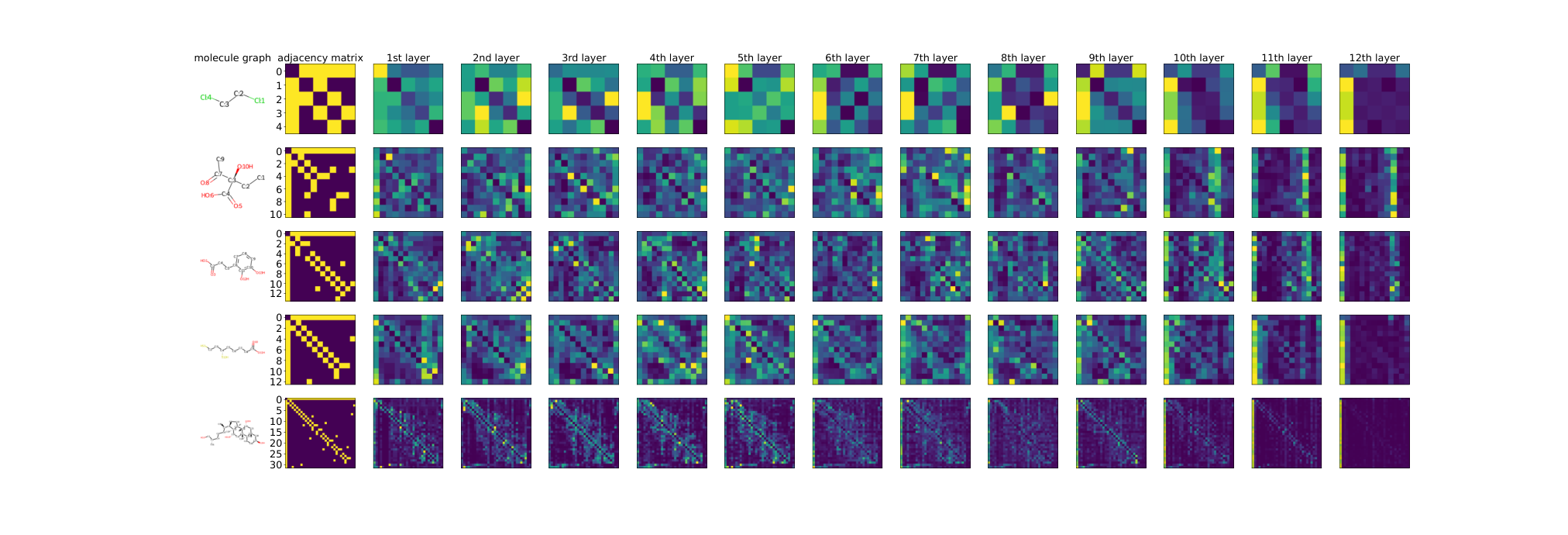
We visualize attention map of each layer on molecules with various size. We take average over the attention map of 32 heads from GRPE-Standard trained on graph regression task on PCQM4Mv2 dataset. Note that, the first node is virtual node (with index zero), and its attention map and adjacency is represented at the first row and column. Figure 4 shows that our method attend to neighboring nodes at lower layers. As layer goes deeper, attention map attends to virtual node with higher attention on the first column. This shows that each layer focuses on the entire graph rather than each node.
Conclusion
We studied the problem of positional encoding for representing structural information of the given graph better, specifically, by adding node-topology and node-edge relations to the model. We validated the effectiveness of our approach, both quantitatively and qualitatively, in various tasks of diverse dataset sizes and characteristics, e.g., HIV replication prediction from molecule graphs (MolHIV) or semi-supervised clustering on synthetic graphs (CLUSTER).
References
- Beani et al. (2021) Beani, D.; Passaro, S.; Létourneau, V.; Hamilton, W.; Corso, G.; and Liò, P. 2021. Directional graph networks. In International Conference on Machine Learning, 748–758. PMLR.
- Belkin and Niyogi (2003) Belkin, M.; and Niyogi, P. 2003. Laplacian eigenmaps for dimensionality reduction and data representation. Neural computation, 15(6): 1373–1396.
- Bresson and Laurent (2017) Bresson, X.; and Laurent, T. 2017. Residual gated graph convnets. arXiv preprint arXiv:1711.07553.
- Brossard, Frigo, and Dehaene (2020) Brossard, R.; Frigo, O.; and Dehaene, D. 2020. Graph convolutions that can finally model local structure. arXiv preprint arXiv:2011.15069.
- Cai et al. (2021) Cai, T.; Luo, S.; Xu, K.; He, D.; Liu, T.-y.; and Wang, L. 2021. Graphnorm: A principled approach to accelerating graph neural network training. In International Conference on Machine Learning, 1204–1215. PMLR.
- Corso et al. (2020) Corso, G.; Cavalleri, L.; Beaini, D.; Liò, P.; and Veličković, P. 2020. Principal neighbourhood aggregation for graph nets. arXiv preprint arXiv:2004.05718.
- Devlin et al. (2018) Devlin, J.; Chang, M.-W.; Lee, K.; and Toutanova, K. 2018. Bert: Pre-training of deep bidirectional transformers for language understanding. arXiv preprint arXiv:1810.04805.
- Dwivedi and Bresson (2020) Dwivedi, V. P.; and Bresson, X. 2020. A generalization of transformer networks to graphs. arXiv preprint arXiv:2012.09699.
- Dwivedi et al. (2020) Dwivedi, V. P.; Joshi, C. K.; Laurent, T.; Bengio, Y.; and Bresson, X. 2020. Benchmarking graph neural networks. arXiv preprint arXiv:2003.00982.
- Gilmer et al. (2017) Gilmer, J.; Schoenholz, S. S.; Riley, P. F.; Vinyals, O.; and Dahl, G. E. 2017. Neural message passing for quantum chemistry. In International conference on machine learning, 1263–1272. PMLR.
- He et al. (2016) He, K.; Zhang, X.; Ren, S.; and Sun, J. 2016. Deep residual learning for image recognition. In Proceedings of the IEEE conference on computer vision and pattern recognition, 770–778.
- Hu et al. (2020) Hu, W.; Fey, M.; Zitnik, M.; Dong, Y.; Ren, H.; Liu, B.; Catasta, M.; and Leskovec, J. 2020. Open graph benchmark: Datasets for machine learning on graphs. arXiv preprint arXiv:2005.00687.
- Hussain et al. (2021) Hussain; Shamim, M.; Zaki; J, M.; and Subramanian, D. 2021. Edge-augmented graph transformers: Global self-attention is enough for graphs. arXiv preprint arXiv:2108.03348.
- Kipf and Welling (2016) Kipf, T. N.; and Welling, M. 2016. Semi-supervised classification with graph convolutional networks. arXiv preprint arXiv:1609.02907.
- Kreuzer et al. (2021) Kreuzer, D.; Beaini, D.; Hamilton, W. L.; Létourneau, V.; and Tossou, P. 2021. Rethinking Graph Transformers with Spectral Attention. arXiv preprint arXiv:2106.03893.
- Le et al. (2021) Le, T.; Bertolini, M.; Noé, F.; and Clevert, D.-A. 2021. Parameterized hypercomplex graph neural networks for graph classification. arXiv preprint arXiv:2103.16584.
- Li et al. (2020) Li, G.; Xiong, C.; Thabet, A.; and Ghanem, B. 2020. Deepergcn: All you need to train deeper gcns. arXiv preprint arXiv:2006.07739.
- Rong et al. (2020) Rong, Y.; Bian, Y.; Xu, T.; Xie, W.; Wei, Y.; Huang, W.; and Huang, J. 2020. Self-supervised graph transformer on large-scale molecular data. arXiv preprint arXiv:2007.02835.
- Shaw, Uszkoreit, and Vaswani (2018) Shaw, P.; Uszkoreit, J.; and Vaswani, A. 2018. Self-attention with relative position representations. arXiv preprint arXiv:1803.02155.
- Vaswani et al. (2017) Vaswani, A.; Shazeer, N.; Parmar, N.; Uszkoreit, J.; Jones, L.; Gomez, A. N.; Kaiser, Ł.; and Polosukhin, I. 2017. Attention is all you need. In Advances in neural information processing systems, 5998–6008.
- Veličković et al. (2017) Veličković, P.; Cucurull, G.; Casanova, A.; Romero, A.; Lio, P.; and Bengio, Y. 2017. Graph attention networks. arXiv preprint arXiv:1710.10903.
- Xu et al. (2018) Xu, K.; Hu, W.; Leskovec, J.; and Jegelka, S. 2018. How powerful are graph neural networks? arXiv preprint arXiv:1810.00826.
- Ying et al. (2021) Ying, C.; Cai, T.; Luo, S.; Zheng, S.; Ke, G.; He, D.; Shen, Y.; and Liu, T.-Y. 2021. Do Transformers Really Perform Bad for Graph Representation? arXiv preprint arXiv:2106.05234.