1Introduction

marginparsep has been altered.
topmargin has been altered.
marginparpush has been altered.

The page layout violates the ICML style.

Please do not change the page layout, or include packages like geometry, savetrees, or fullpage, which change it for you.

We’re not able to reliably undo arbitrary changes to the style. Please remove the offending package(s), or layout-changing commands and try again.

Coordinate Descent Methods for Fractional Minimization

Ganzhao Yuan ^*¹

^†^†footnotetext: ¹Peng Cheng Laboratory, China. Correspondence to: Ganzhao Yuan <yuangzh@pcl.ac.cn>.

Abstract

We consider a class of structured fractional minimization problems, in which the numerator part of the objective is the sum of a differentiable convex function and a convex non-smooth function, while the denominator part is a convex or concave function. This problem is difficult to solve since it is non-convex. By exploiting the structure of the problem, we propose two Coordinate Descent (CD) methods for solving this problem. The proposed methods iteratively solve a one-dimensional subproblem globally, and they are guaranteed to converge to coordinate-wise stationary points. In the case of a convex denominator, under a weak locally bounded non-convexity condition, we prove that the optimality of coordinate-wise stationary point is stronger than that of the standard critical point and directional point. Under additional suitable conditions, CD methods converge Q-linearly to coordinate-wise stationary points. In the case of a concave denominator, we show that any critical point is a global minimum, and CD methods converge to the global minimum with a sublinear convergence rate. We demonstrate the applicability of the proposed methods to some machine learning and signal processing models. Our experiments on real-world data have shown that our method significantly and consistently outperforms existing methods in terms of accuracy.

1 Introduction

Fractional optimization, referring to the problem of minimizing or maximizing an objective involving one or more ratios of functions, has been extensively studied for decades. Fractional optimization problem is widely used in machine learning, signal processing, economics, wireless communication and many other fields. Three classes of factional optimization problems for minimizing the ratio of two functions are extensively investigated in the literature. They are named according to the functions in the numerator and denominator: (i) linear fractional problems if both functions are linear; (ii) convex-convex fractional problems if both functions are convex; (iii) convex-concave fractional problems if the numerator is convex and the denominator is concave. We refer the readers to Stancu-Minasian 2012; Schaible 1995 for an overview.

This paper mainly focuses on the following convex-convex or convex-concave Fractional Minimization Problem (FMP) (‘ $\triangleq$ ’ means define):

\displaystyle\bar{\mathbf{x}}\in\arg\min_{\mathbf{x}\in\mathbb{R}^{n}}~F(\mathbf{x})\triangleq\frac{f(\mathbf{x})+h(\mathbf{x})}{g(\mathbf{x})}.

(1)

We impose the following assumptions on Problem (1) throughout this paper. (A-i) $F(\mathbf{x})$ only takes finite values, and it always holds that: $f(\mathbf{x})+h(\mathbf{x})\geq 0$ and $g(\mathbf{x})>0$ for all $\mathbf{x}$ . (A-ii) $f(\cdot)$ is convex and differentiable, and its gradient is coordinate-wise Lipschitz continuous with constant $\mathbf{c}_{i}\geq 0$ that Nesterov 2012; Nesterov 2003:

\displaystyle\textstyle f(\mathbf{x}+\eta e_{i})\leq\mathcal{Q}_{i}(\mathbf{x},\eta)\triangleq f(\mathbf{x})+\nabla_{i}f(\mathbf{x})\eta+\frac{\mathbf{c}_{i}}{2}\eta^{2}

(2)

$\forall\mathbf{x},\eta,i=1,...,n$ . Here $\mathbf{c}\in\mathbb{R}^{n}$ , and $e_{i}\in\mathbb{R}^{n}$ is an indicator vector with one on the $i$ -th entry and zero everywhere else. (A-iii) $h(\cdot)$ is convex and coordinate-wise separable with $h(\mathbf{x})=\sum_{i=1}^{n}h_{i}(\mathbf{x}_{i})$ . Typical examples of $h(\mathbf{x})$ are the $\ell_{1}$ norm function and the bound constrained function. (A-iv) The denominator $g(\cdot)$ is either (i) a convex but not necessarily differentiable function or (ii) a concave and differentiable function. Furthermore, $g(\cdot)$ has some special structure such that one of the following one-dimensional subproblems can be solved exactly and efficiently:

		$\displaystyle\textstyle\min_{\eta}\frac{\varrho+\rho\eta+\frac{\mathbf{c}_{i}}{2}\eta^{2}+h_{i}(\mathbf{x}+\eta e_{i})}{g(\mathbf{x}+\eta e_{i})}$
		$\displaystyle\textstyle\min_{\eta}\varrho+\rho\eta+\frac{\mathbf{c}_{i}}{2}\eta^{2}+h_{i}(\mathbf{x}+\eta e_{i})-\gamma g(\mathbf{x}+\eta e_{i})$

for any $\varrho\in\mathbb{R}$ , $\rho\in\mathbb{R}$ , and $\gamma\in\mathbb{R}$ . Problem (1) captures a variety of applications of interest, e.g., the sparse recovery problem Li et al. 2022; Li & Zhang 2022, the independent component analysis Hyvärinen & Oja 1997, the $\ell_{p}$ norm eigenvalue problem, the regularized total least squares problem Beck et al. 2006; Amaral & Barahona 2005, and the transmit beamforming Sidiropoulos et al. 2006.

Coordinate Descent (CD) is an iterative algorithm that successively performs minimization along coordinate directions. Due to its simplicity and efficiency, it has been used for many years on the structured high dimensional machine learning and data mining applications including support vector machines Hsieh et al. 2008, non-negative matrix factorization Hsieh & Dhillon 2011, LASSO Tseng & Yun 2009. Its iteration complexity for convex problems has been well-studied Nesterov 2012; Lu & Xiao 2015. Recently, its popularity continues to grow due to its strong optimality guarantees and superior empirical performance when it is applied to solve non-convex problems, including compressed sensing Beck & Eldar 2013; Yuan et al. 2020, eigenvalue complementarity problem Patrascu & Necoara 2015, DC minimization problem Yuan 2021, k-means clustering Nie et al. 2021, sparse phase retrieval Shechtman et al. 2014. To the best of our knowledge, this is the first time to apply CD methods for solving FMPs and study their theoretical properties and empirical behaviors.

Contributions. The contributions of this paper are as follows: (i) We propose two CD methods for solving FMPs. The proposed methods iteratively solve a one-dimensional subproblem globally until convergence. See Section 4. (ii) For convex-convex FMPs, we prove that under suitable conditions the proposed CD methods find stronger coordinate-wise stationary points than existing methods, and they converge linearly. For convex-concave FMPs, we prove that CD methods converge to the global optimal solutions with a sublinear convergence rate. See Section 5. (iii) We demonstrate the applicability of the CD methods to the applications of sparse recovery and $\ell_{p}$ norm eigenvalue problem. We show that the exact minimizer of each coordinate can be obtained by using an elaborate breakpoint searching procedure. Our experiments on real-world data have shown that our methods significantly and consistently outperforms existing approaches in terms of accuracy. See Section 6.

Notations. We use boldface lowercase letters and boldface uppercase letters to denote vectors and matrices, respectively. The Euclidean inner product between $\mathbf{x}$ and $\mathbf{y}$ is denoted by $\langle\mathbf{x},\mathbf{y}\rangle$ or $\mathbf{x}^{T}\mathbf{y}$ . We define $\|\mathbf{x}\|=\|\mathbf{x}\|_{2}=\sqrt{\langle\mathbf{x},\mathbf{x}\rangle}$ . $\mathbf{x}_{i}$ is the $i$ -th element of the vector $\mathbf{x}$ . We define $\|\mathbf{d}\|_{\mathbf{c}}^{2}\triangleq\sum_{i}\mathbf{c}_{i}\mathbf{d}_{i}^{2}$ . $\mathbf{I}$ is the identity matrix of suitable size. $\text{dist}(\Omega,\Omega^{\prime})\triangleq\inf_{\mathbf{v}\in\Omega,\mathbf{v}^{\prime}\in\Omega^{\prime}}\|\mathbf{v}-\mathbf{v}^{\prime}\|$ denotes the distance between two sets.

2 Applications

A wide range of machine learning and signal processing models can be formulated as Problem (1). We briefly review two instances as follows.

$\bullet$ Application I: Sparse Recovery Li et al. 2022; Li & Zhang 2022; Gotoh et al. 2018; Bi et al. 2014. It is a signal processing technique, which can effectively acquire and reconstruct the signal by finding the solution of the underdetermined linear system. Given a design matrix $\mathbf{G}\in\mathbb{R}^{m\times n}$ and an observation vector $\mathbf{y}\in\mathbb{R}^{m}$ , sparse recovery can be formulated as the following FMP Li et al. 2022:

\displaystyle\textstyle\min_{\mathbf{x}}~\frac{\frac{1}{2}\|\mathbf{G}\mathbf{x}-\mathbf{y}\|_{2}^{2}+\gamma\|\mathbf{x}\|_{1}}{\gamma\sum_{j=1}^{k}|\mathbf{x}_{[j]}|},s.t.\|\mathbf{x}\|_{\infty}\leq\vartheta,

(3)

where $\mathbf{x}_{[i]}$ is the $i$ -th largest component of $\mathbf{x}$ in magnitude, and $\gamma>0,\vartheta>0$ are given parameters.

$\bullet$ Application II: $\ell_{p}$ Norm Eigenvalue Problem. Given arbitrary data matrices $\mathbf{G}\in\mathbb{R}^{m\times n}$ and $\mathbf{Q}\in\mathbb{R}^{n\times n}$ with $\mathbf{Q}\succ\mathbf{0}$ , it aims at solving the following problem:

\displaystyle\bar{\mathbf{v}}=\arg\max_{\mathbf{v}}\|\mathbf{G}\mathbf{v}\|_{p},~s.t.~\mathbf{v}^{T}\mathbf{Q}\mathbf{v}=1

(4)

with $p\geq 1$ . When $p=4$ and $\mathbf{Q}=\mathbf{I}$ , Problem (4) reduces to the Independent Component Analysis (ICA) Hyvärinen & Oja 2000; Zhai et al. 2020; when $p=1$ and $\mathbf{Q}=\mathbf{I}$ , Problem (4) is the $\ell_{1}$ PCA problem Kim & Klabjan 2019. We have the following equivalent unconstrained FMPs:

	$\displaystyle\textstyle\bar{\mathbf{x}}=\arg\min_{\mathbf{x}}~\frac{\mathbf{x}^{T}\mathbf{Q}\mathbf{x}+\gamma_{1}}{\\|\mathbf{G}\mathbf{x}\\|_{p}+\gamma_{2}},$		(5)
	$\displaystyle\textstyle\text{or}~\bar{\mathbf{x}}=\arg\min_{\mathbf{x}}~\frac{\mathbf{x}^{T}\mathbf{Q}\mathbf{x}+\gamma_{3}}{\\|\mathbf{G}\mathbf{x}\\|^{2}_{p}+\gamma_{4}}.$		(6)

Here, $\gamma_{1}$ , $\gamma_{2}$ , $\gamma_{3}$ , $\gamma_{4}$ can be any nonnegative constant. The optimal solution to Problem (4) can be computed as $\bar{\mathbf{v}}=\pm\bar{\mathbf{x}}\cdot(\bar{\mathbf{x}}^{T}\mathbf{Q}\bar{\mathbf{x}})^{-\frac{1}{2}}$ . Refer to Section D.1 in the Appendix for detailed discussions.

3 Related Work

We present some related fractional optimization / minimization algorithms.

(i) Dinkelbach’s Parametric Algorithm (DPA) Dinkelbach 1967 is one of the classical approaches for fractional optimization, which deals with Problem (1) by solving its associated parametric problem. By this approach, Problem (1) has an optimal solution $\mathbf{x}\in\mathbb{R}^{n}$ if and only if $\mathbf{x}$ is an optimal solution to the following problem: $\min_{\mathbf{x}}f(\mathbf{x})+h(\mathbf{x})-\bar{\lambda}g(\mathbf{x})$ , where $\bar{\lambda}=\frac{f(\bar{\mathbf{x}})+h(\bar{\mathbf{x}})}{g(\bar{\mathbf{x}})}$ . However, the optimal objective value $\bar{\lambda}$ is unknown in general. Iterative procedures are considered to remedy this issue. DPA generates a sequence $\{\mathbf{x}^{t}\}$ as: $\mathbf{x}^{t+1}=\arg\min_{\mathbf{x}}~f(\mathbf{x})+h(\mathbf{x})-\lambda^{t}g(\mathbf{x})$ , where $\lambda^{t}$ is renewed via $\lambda^{t}=\frac{f(\mathbf{x}^{t})+h(\mathbf{x}^{t})}{g(\mathbf{x}^{t})}$ . Note that the computational cost of solving the subproblem could be expensive since it is non-convex in general.

(ii) Proximal Gradient Algorithm (PGA) Bot & Csetnek 2017 has been proposed for a similar class of fractional optimization problems where the denominator $g(\mathbf{x}^{t})$ is differentiable, and can be suitably applied to Problem (1). The resulting algorithm generates a sequence $\{\mathbf{x}^{t}\}$ as: $\mathbf{x}^{t+1}=\arg\min_{\mathbf{x}}f(\mathbf{x})+h(\mathbf{x})-\lambda^{t}\langle\nabla g(\mathbf{x}^{t}),\mathbf{x}-\mathbf{x}^{t}\rangle+\frac{1}{2\eta^{t}}\|\mathbf{x}-\mathbf{x}^{t}\|_{2}^{2}$ , where $\eta^{t}>0$ and $\lambda^{t}=F(\mathbf{x}^{t})$ .

(iii) Proximal Gradient-Subgradient Algorithm (PGSA) Li & Zhang 2022; Li et al. 2022 assumes that $\nabla f(\cdot)$ is Lipschitz continuous with constant $L$ that: $\forall\mathbf{x},\mathbf{y},~f(\mathbf{x})\leq\mathcal{U}(\mathbf{x};\mathbf{y})\triangleq f(\mathbf{y})+\langle\nabla f(\mathbf{y}),\mathbf{x}-\mathbf{y}\rangle+\frac{L}{2}\|\mathbf{y}-\mathbf{x}\|_{2}^{2}$ , and generates the new iterate using: $\mathbf{x}^{t+1}=\arg\min_{\mathbf{x}}~h(\mathbf{x})+\mathcal{U}(\mathbf{x};\mathbf{x}^{t})-\lambda^{t}\langle\mathbf{g}^{t},\mathbf{x}-\mathbf{x}^{t}\rangle$ , with $\mathbf{g}^{t}\in\partial g(\mathbf{x}^{t}),~\lambda^{t}=F(\mathbf{x}^{t})$ .

(iv) Quadratic Transform Parametric Algorithm (QTPA) Shen & Yu 2018a; Shen & Yu 2018b introduces an additional variable $\beta\in\mathbb{R}$ and converts Problem (1) into the following equivalent variational reformulation: $\min_{\mathbf{x}}\frac{-g(\mathbf{x})}{f(\mathbf{x})+h(\mathbf{x})}\Leftrightarrow\min_{\mathbf{x},\beta}\beta^{2}(f(\mathbf{x})+h(\mathbf{x}))-2\beta\sqrt{g(\mathbf{x})}$ . Similar to DPA, it generates a sequence $\{\mathbf{x}^{t}\}$ as: $\mathbf{x}^{t+1}=\arg\min_{\mathbf{x}}(\beta^{t})^{2}(f(\mathbf{x})+h(\mathbf{x}))-2\beta^{t}\sqrt{g(\mathbf{x})}$ , where $\beta^{t}$ is renewed via $\beta^{t}={\sqrt{g(\mathbf{x}^{t})}}/{(f(\mathbf{x}^{t})+h(\mathbf{x}^{t}))}$ . Note that this method is originally designed for solving multiple-ratio FMPs.

(v) Charnes-Cooper Transform Algorithm (CCTA) converts the original linear-fractional programming problem to a standard linear programming problem Charnes & Cooper 1962. Using the transformation $\mathbf{y}=\frac{\mathbf{x}}{g(\mathbf{x})}$ , $t=\frac{1}{g(\mathbf{x})}$ , one can convert Problem (1) into: $\min_{t,\mathbf{y}}tf(\mathbf{y}/t)+th(\mathbf{y}/t),~s.t.~tg(\mathbf{y}/t)=1$ .

(vi) Other fractional optimization algorithms. A number of other fractional optimization algorithms have been studied in the literature. PGSA with line search is developed for possible acceleration for Problem (1) Li et al. 2022; An extrapolated proximal subgradient algorithm was proposed for solving a similar class of fractional optimization problems Bot et al. 2021.

It is shown that any accumulation points of the sequence generated by all the algorithms above are critical points of Problem (1).

4 Proposed Coordinate Descent Methods

This section presents four variants of Coordinate Descent (CD) methods for solving the Fractional Minimization Problem (FMP) in Problem (1).

$\blacktriangleright$ Raw Coordinate Descent. In the $t$ -th iteration of CD method, we minimize $F(\cdot)$ with respect to the $i^{t}$ coordinate while keeping the remaining coordinates $\{\mathbf{x}^{t}_{j}\}_{j\neq i^{t}}$ fixed. In other words, we solve the following one-dimensional subproblem: $\bar{\eta}^{t}\in\arg\min_{\eta\in\mathbb{R}}~\frac{f(\mathbf{x}^{t}+\eta e_{i^{t}})+h(\mathbf{x}^{t}+\eta e_{i^{t}})}{g(\mathbf{x}^{t}+\eta e_{i^{t}})}$ and then update the solution via $\mathbf{x}^{t+1}=\mathbf{x}^{t}+\bar{\eta}^{t}\cdot e_{i^{t}}$ . However, when $f(\cdot)$ and $g(\cdot)$ are complicated, this one-dimensional problem could be still difficult to solve. Some majorization or approximation techniques are needed to remedy this issue.

$\blacktriangleright$ Parametric Subgradient Coordinate Descent is based on the parametric problem of Problem (1): $\min_{\mathbf{x}}f(\mathbf{x})+h(\mathbf{x})-\lambda^{t}g(\mathbf{x})$ with $\lambda^{t}=F(\mathbf{x}^{t})$ is the current estimate of the objective value. When $g(\cdot)$ is convex, we have:

\displaystyle-g(\mathbf{x}+\eta e_{i})\leq\mathcal{G}_{i^{t}}(\mathbf{x}^{t},\eta)\triangleq-g(\mathbf{x}^{t})-\langle\partial g(\mathbf{x}^{t}),\eta e_{i}\rangle.

(7)

If we replace $f(\mathbf{x}^{t}+\eta e_{i^{t}})$ and $-g(\mathbf{x}^{t}+\eta e_{i^{t}})$ with their majorization functions $\mathcal{Q}_{i^{t}}(\mathbf{x}^{t},\eta)$ and $\mathcal{G}_{i^{t}}(\mathbf{x}^{t},\eta)$ while keep the term $h(\cdot)$ unchanged, we have:

	$\displaystyle\textstyle\bar{\eta}^{t}$	$\displaystyle\in\textstyle\arg\min_{\eta}\mathcal{Q}_{i}(\mathbf{x}^{t},\eta)+h(\mathbf{x}^{t}+\eta e_{i})-\lambda^{t}\mathcal{G}_{i^{t}}(\mathbf{x}^{t},\eta)$
	$\displaystyle\textstyle\mathbf{x}^{t+1}$	$\displaystyle=\textstyle\mathbf{x}^{t}+\bar{\eta}^{t}\cdot e_{i^{t}}.$

However, the upper bound which only uses the subgradient of the nonconvex function $(-g(\mathbf{x}^{t}))$ in (7) could be loose, and it results in weak optimality of critical points for convex-convex FMPs Li & Zhang 2022; Li et al. 2022.

$\blacktriangleright$ Fractional Coordinate Descent is rooted in the original fractional minimization function. It replaces $f(\mathbf{x}^{t}+\eta e_{i^{t}})$ with its majorization (upper-bound) $\mathcal{Q}_{i^{t}}(\mathbf{x}^{t},\eta)$ with $\mathcal{Q}_{i}(\mathbf{x},\eta)\triangleq f(\mathbf{x})+\nabla_{i}f(\mathbf{x})\eta+\tfrac{\mathbf{c}_{i}}{2}\eta^{2}$ while keeps the remaining two terms $h(\cdot)$ and $g(\cdot)$ unchanged, leading to the following iterative procedure:

	$\displaystyle\textstyle\bar{\eta}^{t}$	$\displaystyle\in\textstyle\arg\min_{\eta}\frac{\mathcal{Q}_{i}(\mathbf{x}^{t},\eta)+h(\mathbf{x}^{t}+\eta e_{i})}{g(\mathbf{x}^{t}+\eta e_{i^{t}})}$
	$\displaystyle\textstyle\mathbf{x}^{t+1}$	$\displaystyle=\textstyle\mathbf{x}^{t}+\bar{\eta}^{t}\cdot e_{i^{t}}.$

$\blacktriangleright$ Parametric Coordinate Descent is built upon the associated parametric problem of Problem (1). It replaces $f(\mathbf{x}^{t}+\eta e_{i^{t}})$ with its majorization function $\mathcal{Q}_{i^{t}}(\mathbf{x}^{t},\eta)$ while keeps the term $h(\cdot)$ and $g(\cdot)$ unchanged, resulting in the following updating scheme:

	$\displaystyle\textstyle\bar{\eta}^{t}$	$\displaystyle\in\textstyle\arg\min_{\eta}\mathcal{Q}_{i}(\mathbf{x}^{t},\eta)+h(\mathbf{x}^{t}+\eta e_{i})-\lambda^{t}g(\mathbf{x}^{t}+\eta e_{i^{t}})$
	$\displaystyle\textstyle\mathbf{x}^{t+1}$	$\displaystyle=\textstyle\mathbf{x}^{t}+\bar{\eta}^{t}\cdot e_{i^{t}}.$

$\blacktriangleright$ Choosing the Coordinate to Update. There are mainly several strategies to decide which coordinate to update in the literature Tseng & Yun 2009. (i) Cyclic order rule runs all coordinates in cyclic order $1\rightarrow 2\rightarrow...\rightarrow n\rightarrow 1$ . (ii) Random sampling rule randomly selects one coordinate to update. (iii) Greedy rule picks coordinate $i^{t}$ such that $i^{t}=\arg\max_{j}|\bar{\mathbf{d}}^{t}_{j}|$ where $\bar{\mathbf{d}}^{t}=\arg\min_{\mathbf{d}}\langle\nabla f(\mathbf{x}^{t})-F(\mathbf{x}^{t})\partial g(\mathbf{x}^{t}),\mathbf{d}\rangle+\frac{L}{2}\|\mathbf{d}\|_{2}^{2}+h(\mathbf{x}^{t}+\mathbf{d})$ . Note that it has an equivalent form to the update rule of PGSA (see Section 3) and $\bar{\mathbf{d}}^{t}=\mathbf{0}$ implies that $\mathbf{x}^{t}$ is a stationary point.

Algorithm 1 Coordinate Descent Methods for Fractional Minimization.

Input: an initial feasible solution

\mathbf{x}^{0}

\theta>0

. Set

t=0

for

t=0,1,2,3...T

(S1) Use some strategy to find a coordinate

i^{t}\in\{1,...,n\}

for the

t

-th iteration.

(S2) Define

\displaystyle\textstyle\mathcal{J}_{i}(\mathbf{x},\eta)\triangleq f(\mathbf{x})+\nabla_{i}f(\mathbf{x})\eta+\frac{\mathbf{c}_{i}+\theta}{2}\eta^{2}+h(\mathbf{x}+\eta e_{i}).

Solve one of the following subproblems globally:

\bullet

Option (I): FCD.

\displaystyle\textstyle\bar{\eta}^{t}\in\mathcal{P}_{i^{t}}(\mathbf{x}^{t}),~\mathcal{P}_{i}(\mathbf{x})\triangleq\arg\min_{\eta}\frac{\mathcal{J}_{i}(\mathbf{x},\eta)}{g(\mathbf{x}+\eta e_{i})}.

(8)

\bullet

Option (II): PCD.

	$\displaystyle\textstyle\bar{\eta}^{t}\in\mathcal{P}_{i^{t}}(\mathbf{x}^{t})$		(9)
	$\displaystyle\textstyle\mathcal{P}_{i}(\mathbf{x})\triangleq\arg\min_{\eta}\mathcal{J}_{i}(\mathbf{x},\eta)-F(\mathbf{x})g(\mathbf{x}+\eta e_{i}).$

(S3)

\mathbf{x}^{t+1}=\mathbf{x}^{t}+\bar{\eta}^{t}\cdot e_{i^{t}}~~~(\Leftrightarrow\mathbf{x}_{i^{t}}^{t+1}=\mathbf{x}_{i^{t}}^{t}+\bar{\eta}^{t})

end for

Due to the limitations of Raw Coordinate Descent and Parametric Subgradient Coordinate Descent, we only focus on Fractional Coordinate Descent (FCD) and Parametric Coordinate Descent (PCD) in the sequel. We formally present FCD and PCD in Algorithm 1.

Remarks. (i) Note that we increase $\frac{\mathbf{c}_{i}}{2}\eta^{2}$ to $\frac{\mathbf{c}_{i}+\theta}{2}\eta^{2}$ for the term $\mathcal{J}_{i}(\mathbf{x},\eta)$ . It can be viewed as appending a new proximal term $\frac{\theta}{2}\eta^{2}=\tfrac{\theta}{2}\|(\mathbf{x}^{t}+\eta e_{i^{t}})-\mathbf{x}^{t}\|_{2}^{2}$ to the numerator. As we will see later, the introduction of the proximal term $\tfrac{\theta}{2}\|(\mathbf{x}^{t}+\eta e_{i^{t}})-\mathbf{x}^{t}\|_{2}^{2}$ is critically important for our theoretical analysis. (ii) Setting the derivative of the objective function with respect to $\eta$ to zero, we obtain the following necessary but not sufficient optimality conditions for (8) and (9), respectively:

	$\displaystyle\textstyle\alpha^{t}\triangleq\frac{\mathcal{J}_{i^{t}}(\mathbf{x}^{t},\bar{\eta}^{t})}{g(\mathbf{x}^{t+1})},~~\alpha^{t}\partial_{i^{t}}g(\mathbf{x}^{t+1})\textstyle\in\partial\mathcal{J}_{i^{t}}(\mathbf{x}^{t},\bar{\eta}^{t}),$		(10)
	$\displaystyle\textstyle F(\mathbf{x}^{t})\cdot\partial_{i^{t}}g(\mathbf{x}^{t+1})\textstyle\in\partial\mathcal{J}_{i^{t}}(\mathbf{x}^{t},\bar{\eta}^{t}).$		(11)

(iii) Both FCD and PCD are applicable to solve both convex-convex FMPs and convex-concave FMPs. (iv) For convex-convex FMPs, the subproblems in (8) and (9) are generally non-convex. However, using an elaborate breakpoint searching procedure, its exact minimizer can be obtained. This is the key insight into our CD methods. Existing methods mainly consider multiple-stage convex approximation to handle the convex denominator term, only resulting in weak optimality of critical points Li & Zhang 2022; Li et al. 2022; Dinkelbach 1967. Our methods directly optimize over the denominator term and globally solve a non-convex one-dimensional subproblem. Such a sequential nonconvex approximation strategy leads to stronger optimality conditions. (v) In many situations, the exact minimizer of PCD is easier to obtained than that of FCD since the latter involves an objective function which is of fractional structure.

5 Theoretical Analysis

We now provide some theoretical analysis of Algorithm 1. We treat convex-convex FMPs and convex-concave FMPs separately. Due to space limit, all proofs are placed into the Appendix.

5.1 Technical Preliminaries

We need some tools in non-smooth analysis including Fréchet subdifferential, limiting (Fréchet) subdifferential, and directional derivative Mordukhovich 2006; Rockafellar & Wets. 2009; Bertsekas 2015. For any extended real-valued (not necessarily convex) function $F:\mathbb{R}^{n}\rightarrow(-\infty,+\infty]$ , its domain is defined by $\text{dom}(F)\triangleq\{\mathbf{x}\in\mathbb{R}^{n}:|F(\mathbf{x})|<+\infty\}$ . The Fréchet subdifferential of $F$ at $\mathbf{x}\in\text{dom}(F)$ , denoted as $\hat{\partial}F(\mathbf{x})$ , is defined as $\hat{\partial}{F}(\mathbf{x})\triangleq\{\mathbf{v}\in\mathbb{R}^{n}:\lim\inf_{\mathbf{z}\rightarrow\mathbf{x}}\frac{{F}(\mathbf{z})-{F}(\mathbf{x})-\langle\mathbf{v},\mathbf{z}-\mathbf{x}\rangle}{\|\mathbf{z}-\mathbf{x}\|}\geq 0\}$ . The limiting subdifferential of ${F}(\mathbf{x})$ at $\mathbf{x}\in\text{dom}({F})$ is defined as: $\partial{F}(\mathbf{x})\triangleq\{\mathbf{v}\in\mathbb{R}^{n}:\exists\mathbf{x}^{k}\rightarrow\mathbf{x},{F}(\mathbf{x}^{k})\rightarrow{F}(\mathbf{x}),\mathbf{v}^{k}\in\hat{\partial}{F}(\mathbf{x}^{k})\rightarrow\mathbf{v},\forall k\}$ . Note that $\hat{\partial}{F}(\mathbf{x})\subseteq\partial{F}(\mathbf{x})$ . If $F(\cdot)$ is differentiable at $\mathbf{x}$ , then $\hat{\partial}{F}(\mathbf{x})=\partial{F}(\mathbf{x})=\{\nabla F(\mathbf{x})\}$ with $\nabla F(\mathbf{x})$ being the gradient of $F(\cdot)$ at $\mathbf{x}$ . When $F(\cdot)$ is convex, $\hat{\partial}{F}(\mathbf{x})$ and $\partial{F}(\mathbf{x})$ reduce to the classical subdifferential for convex functions, i.e., $\hat{\partial}{F}(\mathbf{x})=\partial{F}(\mathbf{x})=\{\mathbf{v}\in\mathbf{R}^{n}:F(\mathbf{z})-F(\mathbf{x})-\langle\mathbf{v},\mathbf{z}-\mathbf{x}\rangle\geq 0,\forall\mathbf{z}\in\mathbb{R}^{n}\}$ . Since $\partial h(\mathbf{x})$ is coordinate-wise separable, we use $(\partial h(\mathbf{x}))_{i}$ to denote the subgradient of $h(\mathbf{x})$ at $\mathbf{x}$ for the $i$ -th component. The directional derivative of $F(\cdot)$ at $\mathbf{x}$ in the direction $\mathbf{v}$ is defined (if it exists) by $F^{\prime}(\mathbf{x};\mathbf{v})\triangleq\lim_{t\rightarrow 0^{+}}\frac{1}{t}(F(\mathbf{x}+t\mathbf{v})-F({\mathbf{x}}))$ .

We present two kinds of stationary solutions for the non-convex non-differentiable FMP in (1).

Definition 5.1.

(Critical Point, or C-Point for short) A solution $\check{\mathbf{x}}$ is called a C-point if Li & Zhang 2022: $0\in\partial\nabla f(\check{\mathbf{x}})+\partial h(\check{\mathbf{x}})-F(\check{\mathbf{x}})\cdot\partial g(\check{\mathbf{x}})$ .

Definition 5.2.

(Directional Point, or D-Point for short) A solution $\grave{\mathbf{x}}$ is called a D-point if Pang et al. 2017: $F^{\prime}(\grave{\mathbf{x}};\mathbf{y}-\grave{\mathbf{x}})\geq 0,~\forall\mathbf{y}\in\text{dom}(F)$ .

Remarks. (i) The definition of C-Point differs from the standard one $0\in\hat{\partial}F(\check{\mathbf{x}})$ , and it holds that $\hat{\partial}F(\check{\mathbf{x}})=\frac{\hat{\partial}(g(\check{\mathbf{x}})(f+h)-(f(\check{\mathbf{x}})+h(\check{\mathbf{x}}))g)(\check{\mathbf{x}})}{(g(\check{\mathbf{x}}))^{2}}\subseteq\partial F(\check{\mathbf{x}})$ Li & Zhang 2022. (ii) When $F(\cdot)$ is differentiable, the optimality of C-point is equivalent to that of D-point. (iii) The expression $0\in\partial F(\check{\mathbf{x}})$ is equivalent to $[\nabla f(\check{\mathbf{x}})+\partial h(\check{\mathbf{x}})]\cap[F(\check{\mathbf{x}})\partial g(\check{\mathbf{x}})]\neq\emptyset$ . (iii) The function $g(\cdot)$ need not be differentiable since the sub-differential is always non-empty on convex functions. (iv) All existing methods including DPA, PGA, PGSA, and QTPA as mentioned in Section 3 are only guaranteed to find a C-point of Problem (1).

We make the following assumption which will be used in our theoretical analysis.

Assumption 5.3.

(Boundedness of the Denominator) There exists a constant $\bar{g}>0$ such that $\forall\mathbf{x}\in\{\mathbf{z}~|~F(\mathbf{z})\leq F(\mathbf{x}^{0})\},~g(\mathbf{x})\leq\bar{g}$ .

Remarks. As multiplying the numerator and the denominator of $F(\mathbf{x})$ simultaneously by a positive constant does not change the value of $F(\mathbf{x})$ , Assumption 5.3 is reasonable.

We develop the following useful lemmas for both convex-convex FMPs and convex-concave FMPs.

Lemma 5.4.

(Sufficient Decrease Condition) $F(\mathbf{x}^{t+1})-F(\mathbf{x}^{t})\leq{-\frac{\theta}{2g(\mathbf{x}^{t+1})}\|\mathbf{x}^{t+1}-\mathbf{x}^{t}\|_{2}^{2}}$ .

Remarks. (i) Both FCD and PCD have the same sufficient decrease condition. (ii) The proximal parameter $\theta$ is critically important to guarantee global convergence and convergence rate of our algorithm.

Lemma 5.5.

(Property of FCD) The value of the parameter $\alpha^{t}$ defined in (10) is sandwiched as $F(\mathbf{x}^{t+1})\leq\alpha^{t}\leq F(\mathbf{x}^{t+1})+\sigma(F(\mathbf{x}^{t})-F(\mathbf{x}^{t+1}))\leq\sigma F(\mathbf{x}^{0})$ with $\sigma\triangleq\frac{\max(\mathbf{c})+\theta}{\theta}$ .

We assume that the coordinate $i^{t}$ in each iteration is selected randomly and randomly. Our algorithm generates a random output $\mathbf{x}^{t}$ with $t=0,1,...$ , which depends on the observed realization of the random variable: $\xi^{t-1}\triangleq\{i^{0},~i^{1},...,i^{t-1}\}$ . We use $\mathbb{E}[\cdot]$ to denote the expectation of a random variable.

5.2 Convex-Convex FMPs

This subsection presents some theoretical analysis for Algorithm 1 when the denominator $g(\cdot)$ is convex but not necessarily differentiable.

We first present the following useful definition.

Definition 5.6.

(Globally or Locally $\rho$ -Bounded Non-Convexity) (i) A function $\tilde{g}(\mathbf{x})=-g(\mathbf{x})$ is globally $\rho$ -bounded non-convex if: $\forall\mathbf{x},\mathbf{y},~\tilde{g}(\mathbf{x})\leq\tilde{g}(\mathbf{y})+\langle\partial\tilde{g}(\mathbf{x}),~\mathbf{x}-\mathbf{y}\rangle+\frac{\rho}{2}\|\mathbf{x}-\mathbf{y}\|_{2}^{2}$ with $\rho<+\infty$ . (ii) $\tilde{g}(\mathbf{x})$ is locally $\rho$ -bounded non-convex if $\mathbf{x}$ is defined as some point $\check{\mathbf{x}}$ with $\mathbf{x}\triangleq\check{\mathbf{x}}$ .

Remarks. (i) The definition of globally bounded non-convexity is also known as weakly-convex, semi-convex, or approximate convex in the literature (cf. Allen-Zhu 2018; Böhm & Wright 2021; Li et al. 2021). (ii) By this definition, $(\tilde{g}(\mathbf{x})+\tfrac{\rho}{2}\|x\|_{2}^{2})$ is convex. (iii) Smoothness is not required as convex functions are not necessarily smooth. (iv) It is not hard to verify that $\tilde{g}(\mathbf{x})=-\|\mathbf{G}\mathbf{x}\|_{4}^{2}$ in (6) is concave and globally bounded non-convex, while $\tilde{g}(\mathbf{x})=-\gamma\sum_{j=1}^{k}|\mathbf{x}_{[j]}|$ as in (3) is concave and locally bounded non-convex. See Section D.3 in the Appendix.

5.2.1 Optimality Analysis

We now present two kinds of stationary solution which are novel in this paper.

Definition 5.7.

(Fractional Coordinate-Wise Point, or FCW-Point for short) Given a constant $\theta\geq 0$ . Define $\mathcal{K}_{i}(\mathbf{x},\eta)\triangleq\frac{\mathcal{J}_{i}(\mathbf{x},\eta)}{g(\mathbf{x}+\eta e_{i})}$ . A solution $\ddot{\mathbf{x}}$ is called a FCW-point if: $\mathcal{K}_{i}(\ddot{\mathbf{x}},0)=\min_{\boldsymbol{\eta}_{i}}\mathcal{K}_{i}(\ddot{\mathbf{x}},\boldsymbol{\eta}_{i}),~\forall i=1,...,n$ .

Definition 5.8.

(Parametric Coordinate-Wise Point, or PCW-Point for short) Given a constant $\theta\geq 0$ . Define $\mathcal{M}_{i}(\mathbf{x},\eta)\triangleq\mathcal{J}_{i}(\mathbf{x},\eta)-F(\mathbf{x})g(\mathbf{x}+\eta e_{i})$ . A solution $\dot{\mathbf{x}}$ is called a PCW-point if: $\mathcal{M}_{i}(\dot{\mathbf{x}},0)=\min_{\boldsymbol{\eta}_{i}}\mathcal{M}_{i}(\dot{\mathbf{x}},\boldsymbol{\eta}_{i}),~\forall i=1,...,n$ .

Remarks. Both the FCW-point and the PCW-point use another non-convex problem to characterize their stationary, and they state that if we minimize the majorization/surrogate function $\mathcal{K}_{i}(\ddot{\mathbf{x}},\eta)$ (or $\mathcal{M}_{i}(\dot{\mathbf{x}},\eta)$ ), we can not improve the objective value for $\mathcal{K}_{i}(\ddot{\mathbf{x}},\eta)$ (or $\mathcal{M}_{i}(\dot{\mathbf{x}},\eta)$ ) for all $i$ .

Lemma 5.9.

For any FCW-point $\ddot{\mathbf{x}}$ and any PCW-point $\dot{\mathbf{x}}$ , assume that $\tilde{g}(\mathbf{x})=-g(\mathbf{x})$ is locally $\rho$ -bounded non-convex at the point $\ddot{\mathbf{x}}$ (or $\dot{\mathbf{x}}$ ) with $\rho<+\infty$ . We define $\mathcal{C}(\mathbf{x},\boldsymbol{\eta})\triangleq\frac{1}{2}\|\boldsymbol{\eta}\|^{2}_{\mathbf{c}+\theta}+\frac{\rho}{2}\|\boldsymbol{\eta}\|_{2}^{2}F(\mathbf{x})$ . We have: $\textit{{(i)}}~\forall\boldsymbol{\eta},~F(\ddot{\mathbf{x}})-F(\ddot{\mathbf{x}}+\boldsymbol{\eta})\leq\frac{\mathcal{C}(\ddot{\mathbf{x}},\boldsymbol{\eta})}{g(\ddot{\mathbf{x}}+\boldsymbol{\eta})},~\textit{{(ii)}}~\forall\boldsymbol{\eta},~F(\dot{\mathbf{x}})-F(\dot{\mathbf{x}}+\boldsymbol{\eta})\leq\frac{\mathcal{C}(\dot{\mathbf{x}},\boldsymbol{\eta})}{g(\dot{\mathbf{x}}+\boldsymbol{\eta})}$ .

Remarks. The lemma above essentially implies that the optimality of FCW-point coincides with that of PCW-point; i.e., any FCW-point must be a PCW-point, and vice versa.

We use $\check{\mathbf{x}}$ , $\grave{\mathbf{x}}$ , $\dot{\mathbf{x}}$ , $\ddot{\mathbf{x}}$ , and $\bar{\mathbf{x}}$ to denote a C-point, a D-point, a FCW-point, a PCW-point, and an optimal point, respectively. The following theorem establishes their relations.

Theorem 5.10.

(Optimality Hierarchy between the Optimality Conditions). Based on the the assumption made in Lemma 5.9. The following relations hold: $\{\bar{\mathbf{x}}\}\overset{\textbf{(a)}}{\subseteq}\{\ddot{\mathbf{x}}\}\overset{\textbf{(b)}}{\Leftrightarrow}\{\dot{\mathbf{x}}\}\overset{\textbf{(c)}}{\subseteq}\{\grave{\mathbf{x}}\}\overset{\textbf{(d)}}{\subseteq}\{\check{\mathbf{x}}\}$ .

Remarks. The optimality condition of FCW-point or PCW-point is stronger than that of C-point Li et al. 2022; Li & Zhang 2022; Bot & Csetnek 2017 and D-point Pang et al. 2017 when $(-g(\cdot))$ is $\rho$ -bounded non-convex. We use the following one-dimensional example to clarify this point: $\min_{x}f(\mathbf{x})\triangleq\frac{(x+2)^{2}}{|3x+2|+1}$ . This problem contains three C-points $\{-2,-\tfrac{2}{3},0\}$ and two D-points $\{-2,0\}$ . $x=-2$ is the unique FCW-point since it is the unique global optimal solution for this one-dimensional problem. After some preliminary calculations, one can verify that $x=-2$ is also the unique PCW-point. See Section D.2 in the Appendix.

5.2.2 Convergence Analysis

We first define the approximate FCW-Point and approximate PCW-Point.

Definition 5.11.

(Approximate FCW-Point and Approximate PCW-Point) Given any constant $\epsilon>0$ . Define $\mathcal{J}_{i}(\mathbf{x},\eta)\triangleq f(\mathbf{x})+\nabla_{i}f(\mathbf{x})\eta+\frac{\mathbf{c}_{i}+\theta}{2}\eta^{2}+h(\mathbf{x}+\eta e_{i})$ with $\theta\geq 0$ , $\mathcal{K}_{i}(\mathbf{x},\eta)\triangleq\frac{\mathcal{J}_{i}(\mathbf{x},\eta)}{g(\mathbf{x}+\eta e_{i})}$ , $\mathcal{M}_{i}(\mathbf{x},\eta)\triangleq\frac{\mathcal{J}_{i}(\mathbf{x},\eta)}{g(\mathbf{x}+\eta e_{i})}$ .

(i) A solution $\ddot{\mathbf{x}}$ is called an $\epsilon$ -approximate FCW-point if: $\frac{1}{n}\sum_{i=1}^{n}\text{dist}(0,\arg\min_{\eta}\mathcal{K}_{i}(\ddot{\mathbf{x}},\eta))^{2}\leq\epsilon$ .

(ii) A solution $\dot{\mathbf{x}}$ is called an $\epsilon$ -approximate PCW-point if: $\frac{1}{n}\sum_{i=1}^{n}\text{dist}(0,\arg\min_{\eta}\mathcal{M}_{i}(\dot{\mathbf{x}},\eta))^{2}\leq\epsilon$ .

We now prove the global convergence of Algorithm 1 for convex-convex FMPs.

Proposition 5.12.

(Global Convergence) Assume that $\mathbf{x}^{t}$ is bounded for all $t$ ^➀^➀ ➀ This condition always holds if we impose bound constraints on $\mathbf{x}$ that $\|\mathbf{x}\|_{\infty}\leq\vartheta$ , refer to Problem (3)., any clustering point of the sequence is almost surely a FCW-point (or a PCW-point) of Problem (1). Furthermore, Algorithm 1 finds an $\epsilon$ -approximate FCW-point (or PCW-point) of Problem (1) in at most $T+1$ iterations in the sense of expectation, where $T\leq\lceil\tfrac{2n\bar{g}F(\mathbf{x}^{0})}{\theta\epsilon}\rceil=\mathcal{O}(\epsilon^{-1})$ .

To achieve stronger convergence result for Algorithm 1, we make the following additional assumption.

Assumption 5.13.

(Luo-Tseng Error Bound Luo & Tseng 1993; Tseng & Yun 2009) We define a residual function as $\mathcal{R}(\mathbf{x})\triangleq\frac{1}{n}\sum_{i=1}^{n}|\mathcal{P}_{i}(\mathbf{x})|$ , where $\mathcal{P}_{i}(\mathbf{x})$ is defined in (8) (or (9)). For any $\zeta\geq\min_{\mathbf{x}}F(\mathbf{x})$ , there exist scalars $\delta>0$ and $\varrho>0$ such that:

\displaystyle\text{dist}(\mathbf{x},\mathcal{X})\leq\delta\cdot\mathcal{R}(\mathbf{x}),~\text{whenever}~F(\mathbf{x})\leq\zeta,~\mathcal{R}(\mathbf{x})\leq\varrho.

(12)

Here, $dist(\mathbf{x},\mathcal{X})=\inf_{\mathbf{z}\in\mathcal{X}}\|\mathbf{z}-\mathbf{x}\|$ , $\mathcal{X}$ is the set of the FCW-point (or the PCW-point).

Luo-Tseng error bound has long been a significant topic in all aspects of mathematical optimization. Many optimization problems have been shown to possess the Luo-Tseng error bound property Yue et al. 2019; Dong & Tao 2021. Assumption 5.13 is similar to the classical local proximal error bound assumption in the literature. We note that if $\mathbf{x}^{t}$ is not the FCW-point (or the PCW-point), we have $\mathcal{R}(\mathbf{x}^{t})>0$ . By the boundedness of $\mathbf{x}^{t}$ and $\dot{\mathbf{x}}$ (or $\ddot{\mathbf{x}}$ ), there exists a sufficiently large constant $\delta$ such that $\text{dist}(\mathbf{x}^{t},\mathcal{X})\leq\delta\cdot\mathcal{R}(\mathbf{x}^{t})$ . Thus, Assumption 5.13 is reasonable.

We now establish the convergence rate for Algorithm 1. We have the following two theorems.

Theorem 5.14.

(Convergence Rate of FCD). For any FCW-point $\ddot{\mathbf{x}}$ , we define $\ddot{q}^{t}\triangleq F(\mathbf{x}^{t})-F(\ddot{\mathbf{x}}),~r^{t}\triangleq\frac{1}{2}\|\mathbf{x}^{t}-\ddot{\mathbf{x}}\|_{\bar{\mathbf{c}}}^{2},~\bar{\mathbf{c}}\triangleq\mathbf{c}+\theta$ . Assume that $\tilde{g}(\mathbf{x})=-g(\mathbf{x})$ is globally $\rho$ -bounded non-convex, and $F(\cdot)$ satisfies Assumption 5.13. We define: $\varpi\triangleq\frac{\max(\bar{\mathbf{c}})}{\min(\bar{\mathbf{c}})}\cdot\frac{\rho}{\theta}\cdot F(\mathbf{x}^{0})$ . We have the following inequality: $(1-\varpi)\mathbb{E}_{i^{t}}[r^{t+1}]+\frac{g(\bar{\mathbf{x}})}{n}\ddot{q}^{t+1}\leq(1-\varpi)r^{t}+\frac{\varpi}{n}r^{t}$ . When the proximal parameter $\theta$ is sufficiently large such that $\varpi\leq 1$ , we obtain: $\ddot{q}^{t+1}\leq(\frac{\kappa_{1}}{\kappa_{1}+\kappa_{0}})^{t+1}\ddot{q}^{0}$ , where $\kappa_{0}\triangleq\frac{g(\bar{\mathbf{x}})}{\bar{g}}$ and $\kappa_{1}\triangleq(n+1)\max(\bar{\mathbf{c}})\delta^{2}/\theta$ .

Theorem 5.15.

(Convergence Rate of PCD). For any PCW-point $\dot{\mathbf{x}}$ , we define $\dot{q}^{t}\triangleq F(\mathbf{x}^{t})-F(\dot{\mathbf{x}}),~r^{t}\triangleq\frac{1}{2}\|\mathbf{x}^{t}-\dot{\mathbf{x}}\|_{\bar{\mathbf{c}}}^{2},~\bar{\mathbf{c}}\triangleq\mathbf{c}+\theta$ . Assume that $\tilde{g}(\mathbf{x})=-g(\mathbf{x})$ is globally $\rho$ -bounded non-convex, and $F(\cdot)$ satisfies Assumption 5.13. We define: $\varpi\triangleq\frac{\rho}{\min(\bar{\mathbf{c}})}F(\mathbf{x}^{0})$ . We have the following inequality: $\mathbb{E}_{i^{t}}[(1-\varpi)r^{t+1}]+\frac{\bar{g}}{n}\dot{q}^{t+1}\leq(1-\varpi)r^{t}+\frac{\varpi}{n}r^{t}-\frac{g(\bar{\mathbf{x}})}{n}\dot{q}^{t}+\frac{\bar{g}}{n}\dot{q}^{t}$ . When the proximal parameter $\theta$ is sufficiently large such that $\varpi\leq 1$ , we obtain: $\dot{q}^{t+1}\leq(\frac{\kappa_{1}+1-\kappa_{0}}{\kappa_{1}+1})^{t+1}\dot{q}^{0}$ , where $\kappa_{0}\triangleq\frac{g(\bar{\mathbf{x}})}{\bar{g}}$ and $\kappa_{1}\triangleq(n+1)\max(\bar{\mathbf{c}})\delta^{2}/\theta$ .

Remarks. (i) Algorithm 1 converges to the FCW-point (or the PCW-point) with a Q-linear convergence rate. (ii) We compare the convergence rate of FCD and PCD which depend on $\kappa_{0}$ and $\kappa_{1}$ : $(\frac{\kappa_{1}+1-\kappa_{0}}{\kappa_{1}+1})-(\frac{\kappa_{1}}{\kappa_{1}+\kappa_{0}})=\frac{1}{(\kappa_{1}+\kappa_{0})(\kappa_{1}+1)}[\kappa_{1}(\kappa_{1}+\kappa_{0})+(\kappa_{1}+\kappa_{0})-\kappa_{0}(\kappa_{1}+\kappa_{0})-\kappa_{1}(\kappa_{1}+1)]=\frac{\kappa_{0}(1-\kappa_{0})}{(\kappa_{1}+\kappa_{0})(\kappa_{1}+1)}\geq 0$ , where the inequality holds due to $\kappa_{0}\triangleq\frac{g(\bar{\mathbf{x}})}{\bar{g}}\in(0,1]$ . Thus, the convergence rate of FCD is better than that of PCD in theory.

5.3 Convex-Concave FMPs

This subsection provides some theoretical analysis for Algorithm 1 when the donominator $g(\cdot)$ is concave and differentiable ^➁^➁ ➁ Since any coordinate-wise stationary point is not necessarily the first-order stationary point for non-separable and non-differentiable convex functions Tseng & Yun 2009 as in (9), we further assume that the convex function $(-g(\cdot))$ is differentiable.. Convex-concave FMPs as in Problem 1 can be converted to an equivalent convex program using the Charnes-Cooper transformation Hadjisavvas et al. 2006: $\min_{t,\mathbf{y}}tf(\mathbf{y}/t)+th(\mathbf{y}/t),~s.t.~tg(\mathbf{y}/t)\geq 1$ . However, our CD methods are able to directly solve Problem (1) with exploiting its specific structure.

$\bullet$ Optimality Analysis. We provide some theoretical insights into convex-concave FMP.

Proposition 5.16.

(i) $F(\cdot)$ is quasiconvex that: $F(\alpha\mathbf{x}+(1-\alpha)\mathbf{y})\leq\max(F(\mathbf{x}),F(\mathbf{y})),\forall\alpha\in[0,1],\mathbf{x},\mathbf{y}.$ (ii) Any critical point of Problem (1) is a global minimum.

Remarks. (i) Using an inequality $\forall a\geq 0,b\geq 0,c>0,d>0,~\frac{a+b}{c+d}\leq\max(\frac{a}{c},\frac{b}{d})$ , we prove the quasiconvexity of $F(\cdot)$ . (ii) It is shown that any local minimum of a strictly quasiconvex problem is also a global minimum (cf. section 3.5.5 in Bazaraa et al. 2013). General quasiconvex problems do not enjoy this property while we prove that convex-concave FMPs do.

$\bullet$ Convergence Analysis. We now establish the convergence rate of Algorithm 1.

Theorem 5.17.

(Convergence Rate). For any global optimal solution $\bar{\mathbf{x}}$ -point of Problem (1), we define $q^{t}\triangleq F(\mathbf{x}^{t})-F(\bar{\mathbf{x}}),~r^{t}\triangleq\frac{1}{2}\|\mathbf{x}^{t}-\bar{\mathbf{x}}\|_{\bar{\mathbf{c}}}^{2},~\bar{\mathbf{c}}\triangleq\mathbf{c}+\theta$ . (i) For FCD, we have: $\mathbb{E}_{\xi^{t-1}}[q^{t}]\leq\frac{n(\bar{g}\sigma q^{0}+r^{0})}{g(\bar{\mathbf{x}})t}$ , where $\sigma$ is defined in Lemma 5.5. (ii) For PCD, we have: $\mathbb{E}_{\xi^{t-1}}[q^{t}]\leq\frac{n(\bar{g}q^{0}+r^{0})}{g(\bar{\mathbf{x}})(t+1)}$ .

Remarks. Algorithm 1 converges to the global optimal solutions with a sublinear convergence rate.

6 Implementations and Experiments

We first describe the implementations of Algorithm 1 for solving the sparse recovery problem and the $\ell_{p}$ norm eigenvalue problem, and then provide numerical comparisons against state-of-the-art methods on some real-world data. Since the two CD methods achieve the same optimality condition (refer to Theorem 5.10) and we pay more attention to better optimality/accuracy, we only implement one of them for comparisons.

6.1 Implementations for Sparse Recovery

We observe that Problem (3) is a special case of Problem (1) with $f(\mathbf{x})=\frac{1}{2}\|\mathbf{G}\mathbf{x}-\mathbf{y}\|_{2}^{2}$ , $h(\mathbf{x})=\gamma\|\mathbf{x}\|_{1}+I_{\Delta}(\mathbf{x})$ , and $g(\mathbf{x})=\gamma\sum_{j=1}^{k}|\mathbf{x}|_{[j]}$ , where $I_{\Delta}(\mathbf{x})={\{\begin{array}[]{ll}0,&\hbox{ $\mathbf{x}\in\Delta$;}\\ +\infty,&\hbox{else.}\end{array}\}}$ , $\Delta\triangleq\{\mathbf{x}|\|\mathbf{x}\|_{\infty}\leq\vartheta\}$ . The gradient of $f(\mathbf{x})$ can be computed as: $\nabla f(\mathbf{x})=\mathbf{G}^{T}(\mathbf{G}\mathbf{x}-\mathbf{y})\triangleq\mathbf{g}$ . $\nabla f(\mathbf{x})$ is $L$ -Lipschitz continuous with $L=\|\mathbf{G}\|_{2}^{2}$ and coordinate-wise Lipschitz with $\mathbf{c}_{i}=(\mathbf{G}\mathbf{G}^{T})_{ii},~\forall i$ . The subgradient of $g(\mathbf{x})$ can be computed as $(\partial g(\mathbf{x}))_{i}={\{\begin{array}[]{ll}\text{sign}(\mathbf{x}_{i}),&\hbox{ $i\in\Delta_{k}(\mathbf{x})\text{~and~}\mathbf{x}_{i}\neq 0$;}\\ $[-1,1]$,&\hbox{else.}\end{array}\}}$ , where $\Delta_{k}(\mathbf{x})$ is the index of the largest (in magnitude) $k$ elements of $\mathbf{x}$ . According to Algorithm 1, the update for PCD reduces to solving the following one-dimensional problem: $\textstyle\min_{c_{1}\leq\eta\leq c_{2}}\frac{a}{2}\eta^{2}+\eta b+\gamma\|\mathbf{x}+\eta e_{i}\|_{1}-\tau\sum_{j=1}^{k}|\mathbf{x}+\eta e_{i}|_{[j]}$ , where $a=\mathbf{c}_{i}+\theta$ , $b=\mathbf{g}_{i}$ , $\tau=\gamma F(\mathbf{x}^{t})$ , $c_{1}=-\vartheta-\mathbf{x}_{i}$ , $c_{2}=\vartheta-\mathbf{x}_{i}$ . We choose PCD for comparisons since its subproblem is easier to solve.

$\bullet$ A Breakpoint Searching Procedure for PCD. At first, we drop the bound constraint $c_{1}\leq\eta\leq c_{2}$ . Since the variable $\eta$ only affects the value of $\mathbf{x}_{i}$ , we consider two cases for $\mathbf{x}_{i}+\eta$ . (i) $\mathbf{x}_{i}+\eta$ belongs to the top- $k$ subset. Problem (9) reduces to $\min_{\eta}\frac{a}{2}\eta^{2}+\eta b+\gamma|\mathbf{x}_{i}+\eta|-\tau|\mathbf{x}_{i}+\eta|$ . We consider three cases for the non-smooth term $|\mathbf{x}_{i}+\eta|$ , leading to three breakpoints: $\{-\mathbf{x}_{i},(\tau-\gamma-b)/a,(\gamma-\tau-b)/a\}$ . (ii) $\mathbf{x}_{i}+\eta$ does not belong to the top- $k$ subset. Problem (9) reduces to $\min_{\eta}\eta b+\frac{a}{2}\eta^{2}+\gamma|\mathbf{x}_{i}+\eta|$ . Again, we consider three cases for the term $|\mathbf{x}_{i}+\eta|$ , resulting in three breakpoints: $\{-\mathbf{x}_{i^{t}},(-\gamma-b)/a,~(\gamma-b)/a\}$ . Therefore, Problem (9) contains $5$ different breakpoints $\Theta^{\prime}=\{-\mathbf{x}_{i},(\tau-\gamma-b)/a,(\gamma-\tau-b)/a,(-\gamma-b)/a,~(\gamma-b)/a\}$ without the bound constraint. At last, taking the bound constraint into consideration, we conclude that Problem (9) contains 7 breakpoints $\Theta=\{c_{1},c_{2},\min(c_{2},\max(c_{1},\Theta^{\prime}))\}$ .

Once we have identified all the possible breakpoints / critical points $\Theta$ for the one-dimensional subproblem, we pick the solution that leads to the lowest value as the optimal solution.

$\bullet$ Compared Methods. We compare PCD against the following three methods. For ease of discussion, we only consider $\vartheta=+\infty$ in the sequel. (i) DPA iteratively generates a sequence $\{\mathbf{x}^{t}\}$ as: $\mathbf{x}^{t+1}=\arg\min_{\mathbf{x}}f(\mathbf{x})+\gamma\|\mathbf{x}\|_{1}-\lambda^{t}\langle\mathbf{x}-\mathbf{x}^{t},\partial g(\mathbf{x}^{t})\rangle$ , which is solved by an accelerated proximal gradient method Beck & Teboulle 2009; Nesterov 2003. (ii) PGSA generates the new iterate by: $\mathbf{x}^{t+1}=\arg\min_{\mathbf{x}}\frac{L}{2}\|\mathbf{x}-\mathbf{x}^{t}\|_{2}^{2}+\langle\mathbf{x}-\mathbf{x}^{t},\nabla f(\mathbf{x}^{t})\rangle+f(\mathbf{x}^{t})+\gamma\|\mathbf{x}\|_{1}-F(\mathbf{x}^{t})\langle\mathbf{x}-\mathbf{x}^{t},\partial g(\mathbf{x}^{t})\rangle$ , which reduces a soft-thresholding operator. (iii) Quadratic Transform Parametric Algorithm (QTPA) solves the following problem: $\min_{\mathbf{x}}~f(\mathbf{x})+h(\mathbf{x})-2(\beta^{t})^{-1}\sqrt{g(\mathbf{x})}$ with $\beta^{t}$ is renewed as: $\beta^{t}={\sqrt{g(\mathbf{x}^{t})}}/{[f(\mathbf{x}^{t})+h(\mathbf{x}^{t})]}$ . We consider a proximal gradient-subgradient algorithm Li & Zhang 2022; Bot et al. 2021 to minimize the objective function over $\mathbf{x}$ , leading to the following update: $\mathbf{x}^{t+1}=\arg\min_{\mathbf{x}}\frac{L}{2}\|\mathbf{x}-\mathbf{x}^{t}\|_{2}^{2}+\langle\mathbf{x}-\mathbf{x}^{t},\nabla f(\mathbf{x}^{t})\rangle+f(\mathbf{x}^{t})+\gamma\|\mathbf{x}\|_{1}-2(\beta^{t})^{-1}\langle\mathbf{x}-\mathbf{x}^{t},\partial\breve{g}(\mathbf{x}^{t})\rangle$ , where $\partial\breve{g}(\mathbf{x}^{t})$ is the subgradient of $\sqrt{g(\mathbf{x})}$ which can be computed as $\partial\breve{g}(\mathbf{x})=\frac{1}{2}g(\mathbf{x})^{-1/2}\cdot\partial{g}(\mathbf{x})$ .

6.2 Implementations for $\ell_{p}$ Norm Eigenvalue Problem

We observe that Problem (6) is a special case of Problem (1) with $f(\mathbf{x})=\mathbf{x}^{T}\mathbf{Q}\mathbf{x}+\gamma_{3}$ , $h(\mathbf{x})=0$ , and $g(\mathbf{x})=\|\mathbf{G}\mathbf{x}\|^{2}_{p}+\gamma_{4}$ . We consider the classical ICA problem and choose $p=4$ , $\mathbf{Q}=\mathbf{I}$ . We simply set $\gamma_{3}=\gamma_{4}=0$ . Therefore, we have $F(\mathbf{x})=\frac{\|\mathbf{x}\|_{2}^{2}}{\|\mathbf{G}\mathbf{x}\|_{4}^{2}}$ . The gradient of $f(\mathbf{x})$ can be computed as $\nabla f(\mathbf{x})=2\mathbf{x}$ . $\nabla f(\mathbf{x})$ is coordinate-wise Lipschitz continuous with $\mathbf{c}_{i}=2,~\forall i$ . The gradient of $\mathbf{g}(\mathbf{x})$ can be computed as $\nabla g(\mathbf{x})=2g(\mathbf{x})\cdot\sum_{i=1}^{m}((\mathbf{G}_{i}\mathbf{x})^{3}\mathbf{G}_{i}^{T})$ with $\mathbf{G}_{i}\in\mathbb{R}^{1\times n}$ being the $i$ -the row of $\mathbf{G}$ . According to Algorithm 1, the update for FCD reduces to solving the following one-dimensional problem: $\min_{\eta}\frac{\|\mathbf{x}^{t}\|_{2}^{2}+2\mathbf{x}_{i}\eta+\frac{2+\theta}{2}\eta^{2}}{\sqrt{\|\mathbf{G}(\mathbf{x}^{t}+\eta e_{i^{t}})\|^{4}_{4}}}$ . We choose FCD for comparisons since its subproblem is easier to solve.

$\bullet$ A Breakpoint Searching Procedure for FCD. We note that one-dimensional problem boils down to the following problem: $\min_{\eta}p(\eta)\triangleq\frac{a_{2}\eta^{2}+a_{1}\eta+a_{0}}{\sqrt{b_{4}\eta^{4}+b_{3}\eta^{3}+b_{2}\eta^{2}+b_{1}\eta+b_{0}}}$ with suitable parameters $a_{2},a_{1},a_{0}$ and $b_{4},b_{3},b_{2},b_{1},b_{0}$ . Setting the gradient of $p(\cdot)$ to zero yields: $2a_{2}\eta+a_{1}=p(\eta)\tfrac{1}{2}(b_{4}\eta^{4}+b_{3}\eta^{3}+b_{2}\eta^{2}+b_{1}\eta+b_{0})^{-\frac{1}{2}}\cdot(4b_{4}\eta^{3}+3b_{3}\eta^{2}+2b_{2}\eta+b_{1})$ . After some preliminary calculations, the equation above is equivalent to the following quartic equation: $c_{4}\eta^{4}+c_{3}\eta^{3}+c_{2}\eta^{2}+c_{1}\eta+c_{0}=0$ with suitable parameters $c_{4},c_{3},c_{2},c_{1},c_{0}$ . It can be solved analytically by Lodovico Ferrari’s method (https://en.wikipedia.org/wiki/Quartic_equation).

$\bullet$ Compared Methods. We compare PCD against the following two methods. (i) The power Method Hyvärinen & Oja 2000 solves the original problem $\max_{\mathbf{v}}\|\mathbf{G}\mathbf{v}\|^{4}_{4},~s.t.~\|\mathbf{v}\|=1$ using the following update: $\mathbf{x}^{t+1}=\frac{\partial{g}(\mathbf{x}^{t})}{\|\partial{g}(\mathbf{x}^{t})\|}$ . (i) PGSA generates the new iterate by: $\mathbf{x}^{t+1}=\arg\min_{\mathbf{x}}~\|\mathbf{x}\|_{2}^{2}-F(\mathbf{x}^{t})\langle\mathbf{x}-\mathbf{x}^{t},~\partial g(\mathbf{x}^{t})\rangle=\tfrac{1}{2}F(\mathbf{x}^{t})\partial g(\mathbf{x}^{t})$ . Interestingly, we find that the solution of PGSA and that of the power method only differ by a scale factor. Since the objective function $F(\mathbf{x})\triangleq\frac{\|\mathbf{x}\|_{2}^{2}}{\|\mathbf{G}\mathbf{x}\|^{4}_{2}}$ is scale invariance, these two solutions lead to the same objective value for all iterations.

	DPA	PGSA	QTPA	PCD
e2006-1000-1024	1.874 $\pm$ 0.315	1.929 $\pm$ 0.278	1.923 $\pm$ 0.279	1.530 $\pm$ 0.184
e2006-1000-2048	1.640 $\pm$ 0.118	1.663 $\pm$ 0.172	1.660 $\pm$ 0.177	1.312 $\pm$ 0.061
e2006-1024-1000	2.610 $\pm$ 0.796	2.362 $\pm$ 0.533	2.362 $\pm$ 0.530	1.882 $\pm$ 0.418
e2006-2048-1000	5.623 $\pm$ 4.005	6.576 $\pm$ 4.966	6.593 $\pm$ 4.989	3.068 $\pm$ 1.282
news20-1000-1024	1.750 $\pm$ 0.247	1.403 $\pm$ 0.128	1.402 $\pm$ 0.130	1.168 $\pm$ 0.023
news20-1000-2048	2.043 $\pm$ 0.429	1.424 $\pm$ 0.181	1.426 $\pm$ 0.180	1.207 $\pm$ 0.065
news20-1024-1000	1.856 $\pm$ 0.353	1.488 $\pm$ 0.317	1.487 $\pm$ 0.318	1.195 $\pm$ 0.045
news20-2048-1000	4.997 $\pm$ 0.269	2.664 $\pm$ 0.604	2.559 $\pm$ 0.745	1.394 $\pm$ 0.115
sector-1000-1024	1.864 $\pm$ 0.162	1.337 $\pm$ 0.105	1.337 $\pm$ 0.104	1.160 $\pm$ 0.016
sector-1000-2048	1.780 $\pm$ 0.040	1.293 $\pm$ 0.033	1.293 $\pm$ 0.026	1.148 $\pm$ 0.010
sector-1024-1000	2.039 $\pm$ 0.016	1.485 $\pm$ 0.194	1.486 $\pm$ 0.195	1.193 $\pm$ 0.015
sector-2048-1000	5.041 $\pm$ 1.714	2.477 $\pm$ 1.048	2.475 $\pm$ 1.046	1.409 $\pm$ 0.108
TDT2-1000-1024	1.778 $\pm$ 0.303	1.646 $\pm$ 0.035	1.644 $\pm$ 0.032	1.215 $\pm$ 0.047
TDT2-1000-2048	1.710 $\pm$ 0.045	1.398 $\pm$ 0.029	1.398 $\pm$ 0.028	1.127 $\pm$ 0.016
TDT2-1024-1000	1.984 $\pm$ 0.284	1.555 $\pm$ 0.058	1.552 $\pm$ 0.050	1.206 $\pm$ 0.067
TDT2-2048-1000	4.696 $\pm$ 1.980	3.846 $\pm$ 0.901	3.789 $\pm$ 0.800	1.338 $\pm$ 0.038

Table 1: Comparisons of objective values for solving the spare recovery problem.

(a) e2006-1000-2048

(b) e2006-2048-1000

Figure 1: The convergence curve for solving the sparse recovery problem.

6.3 Experiment Settings

To generate the design/signal matrix $\mathbf{G}$ , we consider four publicly available real-world data sets: ‘e2006tfidf’, ‘news20’, ‘sector’, and ‘TDT2’. We randomly select a subset of examples from the original data sets (http://www.cad.zju.edu.cn/home/dengcai/Data/TextData.html, https://www.csie.ntu.edu.tw/˜cjlin/libsvm/). The size of $\mathbf{G}\in\mathbb{R}^{m\times n}$ are are chosen from the following set $(m,n)\in\{(1000,1024),(1000,2048),(1024,1000),(2048,1000)\}$ . To generate the original $k$ -sparse signal $\bar{\mathbf{x}}$ for the sparse recovery problem, we randomly select a support set $S$ of size $100$ and set $\bar{\mathbf{x}}_{\{1,...,n\}\setminus S}=\mathbf{0}$ , $\bar{\mathbf{x}}_{S}=\text{randn}(|S|,1)$ . We generate the observation vector via $\mathbf{y}=\mathbf{G}\bar{\mathbf{x}}+0.1\|\mathbf{G}\bar{\mathbf{x}}\|\cdot\text{randn}(m,1)$ . All methods are implemented in MATLAB on an Intel 2.6 GHz CPU with 64 GB RAM. We use the Matlab inbuilt function ‘roots’ to solve the quartic equation. We define $\mathbf{w}_{t}\triangleq[{F}(\mathbf{x}^{t})-{F}(\mathbf{x}^{t+1})]/\max(1,{F}(\mathbf{x}^{t}))$ , and let all algorithms run up to $T$ seconds and stop them at iteration $t$ if $\text{mean}([{\mathbf{w}}_{t-\text{min}(t,\upsilon)+1},\mathbf{w}_{t-min(t,\upsilon)+2},...,\mathbf{z}_{t}])\leq\epsilon$ . We use the default value $(\theta,\epsilon,\upsilon,T)=(10^{-6},10^{-10},500,100)$ . All methods are executed 10 times and the average performance is reported. We only use the cyclic order rule to select the coordinate for Algorithm 1. Some Matlab code can be found in the supplemental material.

	PGSA	Power Method	FCD
e2006-1000-1024	12.254 $\pm$ 14.922	12.254 $\pm$ 14.922	6.686 $\pm$ 4.956
e2006-1000-2048	16.896 $\pm$ 14.521	16.896 $\pm$ 14.521	9.436 $\pm$ 6.359
e2006-1024-1000	5.923 $\pm$ 4.485	5.923 $\pm$ 4.485	4.948 $\pm$ 2.631
e2006-2048-1000	16.846 $\pm$ 13.916	16.846 $\pm$ 13.916	11.360 $\pm$ 8.225
news20-1000-1024	112.805 $\pm$ 58.995	112.805 $\pm$ 58.995	78.183 $\pm$ 22.830
news20-1000-2048	125.440 $\pm$ 43.203	125.440 $\pm$ 43.203	120.046 $\pm$ 41.353
news20-1024-1000	99.211 $\pm$ 35.338	99.211 $\pm$ 35.338	80.244 $\pm$ 22.771
news20-2048-1000	138.909 $\pm$ 49.626	138.909 $\pm$ 49.626	108.080 $\pm$ 37.811
sector-1000-1024	60.813 $\pm$ 24.018	60.813 $\pm$ 24.018	50.551 $\pm$ 18.675
sector-1000-2048	139.459 $\pm$ 51.094	139.459 $\pm$ 51.094	96.301 $\pm$ 42.115
sector-1024-1000	83.176 $\pm$ 38.697	83.176 $\pm$ 38.697	48.559 $\pm$ 19.163
sector-2048-1000	104.654 $\pm$ 63.318	104.654 $\pm$ 63.318	78.110 $\pm$ 28.532
TDT2-1000-1024	27.167 $\pm$ 12.705	27.167 $\pm$ 12.705	22.308 $\pm$ 8.171
TDT2-1000-2048	27.480 $\pm$ 15.468	27.480 $\pm$ 15.468	23.225 $\pm$ 12.614
TDT2-1024-1000	32.334 $\pm$ 18.178	32.334 $\pm$ 18.178	21.143 $\pm$ 12.143
TDT2-2048-1000	44.659 $\pm$ 19.775	44.659 $\pm$ 19.775	36.517 $\pm$ 12.689

Table 2: Comparisons of objective values for solving the

\ell_{p}

Norm Eigenvalue Problem with

p=4

(a) e2006-1000-2048

(b) e2006-2048-1000

Figure 2: The convergence curve for solving the

\ell_{p}

Norm Eigenvalue Problem with

p=4

6.4 Experiment Results

Table 1 and Figure 1 show the accuracy and computational efficiency for the sparse recovery problem with setting $k=100$ and $\gamma=0.1/m$ . We make the following observations. (i) The proposed method PCD converges faster than the other methods. (ii) PCD consistently gives the best performance.

Table 2 and Figure 2 show the accuracy and computational efficiency for the $\ell_{p}$ Norm Eigenvalue Problem with $p=4$ . We make the following observations. (i) Both PGSA and the power method present the same accuracy since they are essentially equivalent. (ii) While the other methods get stuck into poor local minima, FCD exploits possible higher-order information of the non-convex function to escape from poor local minima and consistently finds lower objectives. This is consistent with our theory that our methods find stronger stationary points.

References

Allen-Zhu (2018) Allen-Zhu, Z. Natasha 2: Faster non-convex optimization than sgd. Advances in Neural Information Processing Systems, 31:2675–2686, 2018.
Amaral & Barahona (2005) Amaral, P. and Barahona, P. Connections between the total least squares and the correction of an infeasible system of linear inequalities. Linear algebra and its applications, 395:191–210, 2005.
Bazaraa et al. (2013) Bazaraa, M. S., Sherali, H. D., and Shetty, C. M. Nonlinear programming: theory and algorithms. John Wiley & Sons, 2013.
Beck & Eldar (2013) Beck, A. and Eldar, Y. C. Sparsity constrained nonlinear optimization: Optimality conditions and algorithms. SIAM Journal on Optimization, 23(3):1480–1509, 2013.
Beck & Teboulle (2009) Beck, A. and Teboulle, M. A fast iterative shrinkage-thresholding algorithm for linear inverse problems. SIAM journal on imaging sciences, 2(1):183–202, 2009.
Beck et al. (2006) Beck, A., Ben-Tal, A., and Teboulle, M. Finding a global optimal solution for a quadratically constrained fractional quadratic problem with applications to the regularized total least squares. SIAM Journal on Matrix Analysis and Applications, 28(2):425–445, 2006.
Bertsekas (2015) Bertsekas, D. Convex optimization algorithms. Athena Scientific, 2015.
Bi et al. (2014) Bi, S., Liu, X., and Pan, S. Exact penalty decomposition method for zero-norm minimization based on mpec formulation. SIAM Journal on Scientific Computing, 36(4):A1451–A1477, 2014.
Böhm & Wright (2021) Böhm, A. and Wright, S. J. Variable smoothing for weakly convex composite functions. Journal of optimization theory and applications, 188:628–649, 2021.
Bot & Csetnek (2017) Bot, R. I. and Csetnek, E. R. Proximal-gradient algorithms for fractional programming. Optimization, 66(8):1383–1396, 2017.
Bot et al. (2021) Bot, R. I., Dao, M. N., and Li, G. Extrapolated proximal subgradient algorithms for nonconvex and nonsmooth fractional programs. Mathematics of Operations Research, 2021.
Charnes & Cooper (1962) Charnes, A. and Cooper, W. W. Programming with linear fractional functionals. Naval Research logistics quarterly, 9(3-4):181–186, 1962.
Dinkelbach (1967) Dinkelbach, W. On nonlinear fractional programming. Management science, 13(7):492–498, 1967.
Dong & Tao (2021) Dong, H. and Tao, M. On the linear convergence to weak/standard d-stationary points of dca-based algorithms for structured nonsmooth DC programming. J. Optim. Theory Appl., 189(1):190–220, 2021.
Gotoh et al. (2018) Gotoh, J., Takeda, A., and Tono, K. Dc formulations and algorithms for sparse optimization problems. Mathematical Programming, 169(1):141–176, 2018.
Hadjisavvas et al. (2006) Hadjisavvas, N., Komlósi, S., and Schaible, S. S. Handbook of generalized convexity and generalized monotonicity, volume 76. Springer Science & Business Media, 2006.
Hsieh & Dhillon (2011) Hsieh, C.-J. and Dhillon, I. S. Fast coordinate descent methods with variable selection for non-negative matrix factorization. In ACM International Conference on Knowledge Discovery and Data Mining (SIGKDD), pp. 1064–1072, 2011.
Hsieh et al. (2008) Hsieh, C.-J., Chang, K.-W., Lin, C.-J., Keerthi, S. S., and Sundararajan, S. A dual coordinate descent method for large-scale linear svm. In International Conference on Machine Learning (ICML), pp. 408–415, 2008.
Hyvärinen & Oja (1997) Hyvärinen, A. and Oja, E. A fast fixed-point algorithm for independent component analysis. Neural computation, 9(7):1483–1492, 1997.
Hyvärinen & Oja (2000) Hyvärinen, A. and Oja, E. Independent component analysis: algorithms and applications. Neural networks, 13(4-5):411–430, 2000.
Kim & Klabjan (2019) Kim, C. and Klabjan, D. A simple and fast algorithm for l1-norm kernel pca. IEEE Transactions on Pattern Analysis and Machine Intelligence, 42(8):1842–1855, 2019.
Li & Zhang (2022) Li, Q. and Zhang, N. First-order algorithms for a class of fractional optimization problems. SIAM Journal on Optimization, 32(1):100–129, 2022.
Li et al. (2022) Li, Q., Shen, L., Zhang, N., and Zhou, J. A proximal algorithm with backtracked extrapolation for a class of structured fractional programming. Applied and Computational Harmonic Analysis, 56:98–122, 2022. ISSN 1063-5203.
Li et al. (2021) Li, X., Chen, S., Deng, Z., Qu, Q., Zhu, Z., and Man-Cho So, A. Weakly convex optimization over stiefel manifold using riemannian subgradient-type methods. SIAM Journal on Optimization, 31(3):1605–1634, 2021.
Lu & Xiao (2015) Lu, Z. and Xiao, L. On the complexity analysis of randomized block-coordinate descent methods. Mathematical Programming, 152(1-2):615–642, 2015.
Luo & Tseng (1993) Luo, Z.-Q. and Tseng, P. Error bounds and convergence analysis of feasible descent methods: a general approach. Annals of Operations Research, 46(1):157–178, 1993.
Mordukhovich (2006) Mordukhovich, B. S. Variational analysis and generalized differentiation i: Basic theory. Berlin Springer, 330, 2006.
Nesterov (2003) Nesterov, Y. Introductory lectures on convex optimization: A basic course, volume 87. Springer Science & Business Media, 2003.
Nesterov (2012) Nesterov, Y. Efficiency of coordinate descent methods on huge-scale optimization problems. SIAM Journal on Optimization, 22(2):341–362, 2012.
Nie et al. (2021) Nie, F., Xue, J., Wu, D., Wang, R., Li, H., and Li, X. Coordinate descent method for k-means. IEEE Transactions on Pattern Analysis and Machine Intelligence, 2021.
Pang et al. (2017) Pang, J., Razaviyayn, M., and Alvarado, A. Computing b-stationary points of nonsmooth DC programs. Mathematics of Operations Research, 42(1):95–118, 2017.
Patrascu & Necoara (2015) Patrascu, A. and Necoara, I. Efficient random coordinate descent algorithms for large-scale structured nonconvex optimization. Journal of Global Optimization, 61(1):19–46, 2015.
Rockafellar & Wets. (2009) Rockafellar, R. T. and Wets., R. J.-B. Variational analysis. Springer Science & Business Media, 317, 2009.
Schaible (1995) Schaible, S. Fractional programming. In Handbook of global optimization, pp. 495–608. Springer, 1995.
Shechtman et al. (2014) Shechtman, Y., Beck, A., and Eldar, Y. C. Gespar: Efficient phase retrieval of sparse signals. IEEE Transactions on Signal Processing, 62(4):928–938, 2014.
Shen & Yu (2018a) Shen, K. and Yu, W. Fractional programming for communication systems - part i: Power control and beamforming. IEEE Transactions on Signal Processing, 66(10):2616–2630, 2018a.
Shen & Yu (2018b) Shen, K. and Yu, W. Fractional programming for communication systems - part II: uplink scheduling via matching. IEEE Transactions on Signal Processing, 66(10):2631–2644, 2018b.
Sidiropoulos et al. (2006) Sidiropoulos, N. D., Davidson, T. N., and Luo, Z.-Q. Transmit beamforming for physical-layer multicasting. IEEE transactions on signal processing, 54(6):2239–2251, 2006.
Stancu-Minasian (2012) Stancu-Minasian, I. M. Fractional programming: theory, methods and applications, volume 409. Springer Science & Business Media, 2012.
Tseng & Yun (2009) Tseng, P. and Yun, S. A coordinate gradient descent method for nonsmooth separable minimization. Mathematical Programming, 117(1):387–423, 2009.
Yuan (2021) Yuan, G. Coordinate descent methods for dc minimization. arXiv preprint arXiv:2109.04228, 2021.
Yuan et al. (2020) Yuan, G., Shen, L., and Zheng, W.-S. A block decomposition algorithm for sparse optimization. In ACM International Conference on Knowledge Discovery and Data Mining (SIGKDD), pp. 275–285, 2020.
Yue et al. (2019) Yue, M., Zhou, Z., and So, A. M. A family of inexact SQA methods for non-smooth convex minimization with provable convergence guarantees based on the luo-tseng error bound property. Math. Program., 174(1-2):327–358, 2019.
Zhai et al. (2020) Zhai, Y., Yang, Z., Liao, Z., Wright, J., and Ma, Y. Complete dictionary learning via l4-norm maximization over the orthogonal group. J. Mach. Learn. Res., 21(165):1–68, 2020.

Appendix

The appendix is organized as follows.
Appendix A presents the proofs for Section 5.1.
Appendix B presents the proofs for Section 5.2.
Appendix C presents the proofs for Section 5.3.
Appendix D presents some additional discussions.

Appendix A Proofs for Section 5.1

A.1 Proof of Lemma 5.4

Proof.

Noticing that $\nabla f(\cdot)$ is coordinate-wise Lipschitz continuous, we have:

\displaystyle f(\mathbf{x}^{t+1})\leq f(\mathbf{x}^{t})+\langle\nabla f(\mathbf{x}^{t}),\mathbf{x}^{t+1}-\mathbf{x}^{t}\rangle+\frac{1}{2}\|\mathbf{x}^{t+1}-\mathbf{x}^{t}\|_{\mathbf{c}}^{2}.

(13)

(a) We first discuss the FCD algorithm. Using the optimality condition of (8), we have:

\displaystyle\frac{f(\mathbf{x}^{t})+\langle\nabla f(\mathbf{x}^{t}),~\mathbf{x}^{t+1}-\mathbf{x}^{t}\rangle+\frac{\mathbf{c}_{i}+\theta}{2}\|\mathbf{x}^{t+1}-\mathbf{x}^{t}\|_{2}^{2}+h(\mathbf{x}^{t+1})}{g(\mathbf{x}^{t+1})}\leq\frac{f(\mathbf{x}^{t})+h(\mathbf{x}^{t})}{g(\mathbf{x}^{t})}.

Combining this inequality with (13), we have:

\displaystyle F(\mathbf{x}^{t+1})+\frac{\theta\|\mathbf{x}^{t+1}-\mathbf{x}^{t}\|_{2}^{2}}{2g(\mathbf{x}^{t+1})}\leq F(\mathbf{x}^{t}).

(b) We now discuss the PCD algorithm. Using the optimality condition of (9) and the fact that $f(\mathbf{x}^{t})+h(\mathbf{x}^{t})=F(\mathbf{x}^{t})\cdot g(\mathbf{x}^{t})$ , we have:

			$\displaystyle f(\mathbf{x}^{t})+\langle\nabla f(\mathbf{x}^{t}),\mathbf{x}^{t+1}-\mathbf{x}^{t}\rangle+\frac{\mathbf{c}_{i}\eta^{2}}{2}+h(\mathbf{x}^{t+1})+\frac{\theta}{2}\eta^{2}-F(\mathbf{x}^{t})g(\mathbf{x}^{t+1})$
		$\displaystyle\leq$	$\displaystyle f(\mathbf{x}^{t})+h(\mathbf{x}^{t})-F(\mathbf{x}^{t})g(\mathbf{x}^{t})=0.$

Rearranging terms, we have:

$\displaystyle 0$	$\displaystyle\leq$	$\displaystyle-f(\mathbf{x}^{t})-\langle\nabla f(\mathbf{x}^{t}),\mathbf{x}^{t+1}-\mathbf{x}^{t}\rangle-\frac{\mathbf{c}_{i}+\theta}{2}\\|\mathbf{x}^{t+1}-\mathbf{x}^{t}\\|_{2}^{2}-h(\mathbf{x}^{t+1})+F(\mathbf{x}^{t})g(\mathbf{x}^{t+1})$
	$\displaystyle\overset{(a)}{\leq}$	$\displaystyle-f(\mathbf{x}^{t+1})-h(\mathbf{x}^{t+1})-\frac{\theta}{2}\\|\mathbf{x}^{t+1}-\mathbf{x}^{t}\\|_{2}^{2}+F(\mathbf{x}^{t})g(\mathbf{x}^{t+1})$
	$\displaystyle\overset{(b)}{=}$	$\displaystyle-F(\mathbf{x}^{t+1})g(\mathbf{x}^{t+1})+F(\mathbf{x}^{t})g(\mathbf{x}^{t+1})-\frac{\theta}{2}\\|\mathbf{x}^{t+1}-\mathbf{x}^{t}\\|_{2}^{2},$

where step $(a)$ uses (13); step $(b)$ uses the definition $f(\mathbf{x}^{t+1})+h(\mathbf{x}^{t+1})=F(\mathbf{x}^{t+1})\cdot g(\mathbf{x}^{t+1})$ . Dividing both sides by $g(\mathbf{x}^{t+1})$ with $g(\mathbf{x}^{t+1})>0$ , we have: $F(\mathbf{x}^{t+1})-F(\mathbf{x}^{t})\leq-\frac{\theta}{2g(\mathbf{x}^{t+1})}\|\mathbf{x}^{t+1}-\mathbf{x}^{t}\|^{2}$ .

∎

A.2 Proof of Lemma 5.5

Proof.

We now give a upper bound for $\alpha^{t}$ . We have:

$\displaystyle\alpha^{t}$	$\displaystyle\triangleq$	$\displaystyle\frac{h(\mathbf{x}^{t+1})+f(\mathbf{x}^{t})+\langle\nabla f(\mathbf{x}^{t}),\mathbf{x}^{t+1}-\mathbf{x}^{t}\rangle+\frac{\mathbf{c}_{i^{t}}+\theta}{2}\\|\mathbf{x}^{t+1}-\mathbf{x}^{t}\\|_{2}^{2}}{g(\mathbf{x}^{t+1})}$
	$\displaystyle\overset{(a)}{\leq}$	$\displaystyle\frac{h(\mathbf{x}^{t+1})+f(\mathbf{x}^{t+1})+\frac{\mathbf{c}_{i^{t}}+\theta}{2}\\|\mathbf{x}^{t+1}-\mathbf{x}^{t}\\|_{2}^{2}}{g(\mathbf{x}^{t+1})}$
	$\displaystyle\overset{(b)}{\leq}$	$\displaystyle F(\mathbf{x}^{t+1})+(F^{t}-F^{t+1})\cdot\frac{(\mathbf{c}_{i^{t}}+\theta)}{\theta},$

where step $(a)$ uses the convexity of $f(\cdot)$ ; step $(b)$ uses the sufficient decrease condition that: $\frac{\theta}{2g(\mathbf{x}^{t+1})}\|\mathbf{x}^{t+1}-\mathbf{x}^{t}\|_{2}^{2}\leq F(\mathbf{x}^{t})-F(\mathbf{x}^{t+1})$ as shown in Lemma 5.4.

We now give a lower bound for $\alpha^{t}$ . We have:

$\displaystyle\alpha^{t}$	$\displaystyle\triangleq$	$\displaystyle\frac{h(\mathbf{x}^{t+1})+f(\mathbf{x}^{t})+\langle\nabla f(\mathbf{x}^{t}),\mathbf{x}^{t+1}-\mathbf{x}^{t}\rangle+\frac{\mathbf{c}_{i^{t}}+\theta}{2}\\|\mathbf{x}^{t+1}-\mathbf{x}^{t}\\|_{2}^{2}}{g(\mathbf{x}^{t+1})}$
	$\displaystyle\overset{(a)}{\geq}$	$\displaystyle\frac{h(\mathbf{x}^{t+1})+f(\mathbf{x}^{t+1})+\frac{\theta}{2}\\|\mathbf{x}^{t+1}-\mathbf{x}^{t}\\|_{2}^{2}}{g(\mathbf{x}^{t+1})}$
	$\displaystyle=$	$\displaystyle F(\mathbf{x}^{t+1})+\frac{\theta\\|\mathbf{x}^{t+1}-\mathbf{x}^{t}\\|_{2}^{2}}{2g(\mathbf{x}^{t+1})}\geq F(\mathbf{x}^{t+1}),$

where step $(a)$ uses the fact that $\nabla f(\mathbf{x})$ is coordinate-wise Lipschitz continuous. ∎

A.3 Proof of Lemma 5.9

Proof.

First, since $\tilde{g}(\mathbf{x})=-g(\mathbf{x})$ is locally $\rho$ -bounded non-convex at the point $\ddot{\mathbf{x}}$ , applying Assumption 5.6 with $\mathbf{x}=\ddot{\mathbf{x}}$ and $\mathbf{y}=\ddot{\mathbf{x}}+\boldsymbol{\eta}$ we have:

			$\displaystyle-g(\ddot{\mathbf{x}})\leq-g(\ddot{\mathbf{x}}+\boldsymbol{\eta})-\langle\ddot{\mathbf{x}}-(\ddot{\mathbf{x}}+\boldsymbol{\eta}),~\partial g(\ddot{\mathbf{x}})\rangle+\frac{\rho}{2}\\|(\ddot{\mathbf{x}}+\boldsymbol{\eta})-\ddot{\mathbf{x}}\\|_{2}^{2}$		(14)
		$\displaystyle\Rightarrow$	$\displaystyle\langle\boldsymbol{\eta},~\partial g(\ddot{\mathbf{x}})\rangle\geq g(\ddot{\mathbf{x}}+\boldsymbol{\eta})-g(\ddot{\mathbf{x}})-\frac{\rho}{2}\\|\boldsymbol{\eta}\\|_{2}^{2}.$		(14)

Second, we have the following inequalities:

$\displaystyle\forall\boldsymbol{\eta},\sum_{i=1}^{n}g(\ddot{\mathbf{x}}+\boldsymbol{\eta}_{i}e_{i})$	$\displaystyle\overset{(a)}{\geq}$	$\displaystyle~\sum_{i=1}^{n}[g(\ddot{\mathbf{x}})+\langle\partial g(\ddot{\mathbf{x}}),~\boldsymbol{\eta}_{i}e_{i}\rangle]$	(15)
	$\displaystyle\overset{(b)}{=}$	$\displaystyle~ng(\ddot{\mathbf{x}})+\langle\partial g(\ddot{\mathbf{x}}),\boldsymbol{\eta}\rangle$
	$\displaystyle\overset{(c)}{\geq}$	$\displaystyle~ng(\ddot{\mathbf{x}})+g(\ddot{\mathbf{x}}+\boldsymbol{\eta})-g(\ddot{\mathbf{x}})-\frac{\rho}{2}\\|\boldsymbol{\eta}\\|_{2}^{2},$

where step $(a)$ uses the convexity of $g(\cdot)$ that: $g(\mathbf{x})-g({\mathbf{x}}+\boldsymbol{\eta}_{i}e_{i})+\langle({\mathbf{x}}+\boldsymbol{\eta}_{i}e_{i})-\mathbf{x},\partial g(\mathbf{x})\rangle\leq 0$ ; step $(b)$ uses $\langle\partial g({\mathbf{x}}),~\boldsymbol{\eta}_{i}e_{i}\rangle=\langle\partial g({\mathbf{x}}),\boldsymbol{\eta}\rangle$ ; step $(c)$ uses (14).

Third, we obtain the following equalities:

$\displaystyle\forall\boldsymbol{\eta},\sum_{i=1}^{n}h(\ddot{\mathbf{x}}+\boldsymbol{\eta}_{i}e_{i})$	$\displaystyle=$	$\displaystyle\sum_{i=1}^{n}\left(h_{i}(\ddot{\mathbf{x}}_{i}+\boldsymbol{\eta}_{i})+\sum_{j\neq i}h_{j}(\ddot{\mathbf{x}}_{j})\right)$	(16)
	$\displaystyle=$	$\displaystyle\sum_{i=1}^{n}\left(h_{i}(\ddot{\mathbf{x}}_{i}+\boldsymbol{\eta}_{i})\right)+\sum_{i=1}^{n}\sum_{j\neq i}h_{j}(\ddot{\mathbf{x}}_{j})$
	$\displaystyle=$	$\displaystyle h(\ddot{\mathbf{x}}+\boldsymbol{\eta})+(n-1)h(\ddot{\mathbf{x}}).$

(a) Since $\ddot{\mathbf{x}}$ is a FCW-point, for all $\boldsymbol{\eta}_{i}\in\mathbb{R}$ , we have:

$\displaystyle\mathcal{K}_{i}(\ddot{\mathbf{x}},0)$	$\displaystyle\leq$	$\displaystyle\mathcal{K}_{i}(\ddot{\mathbf{x}},\boldsymbol{\eta}_{i})$
$\displaystyle\Leftrightarrow~~F(\ddot{\mathbf{x}})$	$\displaystyle\leq$	$\displaystyle\frac{f(\ddot{\mathbf{x}})+\langle\nabla f(\ddot{\mathbf{x}}),~\boldsymbol{\eta}_{i}e_{i}\rangle+h(\ddot{\mathbf{x}}+\boldsymbol{\eta}_{i}e_{i})+\frac{\mathbf{c}_{i}+\theta}{2}\boldsymbol{\eta}_{i}^{2}}{g(\ddot{\mathbf{x}}+\boldsymbol{\eta}_{i}e_{i})}$
$\displaystyle\Leftrightarrow~~F(\ddot{\mathbf{x}})g(\ddot{\mathbf{x}}+\boldsymbol{\eta}_{i}e_{i})$	$\displaystyle\leq$	$\displaystyle f(\ddot{\mathbf{x}})+\langle\nabla f(\ddot{\mathbf{x}}),~\boldsymbol{\eta}_{i}e_{i}\rangle+h(\ddot{\mathbf{x}}+\boldsymbol{\eta}_{i}e_{i})+\frac{\mathbf{c}_{i}+\theta}{2}\boldsymbol{\eta}_{i}^{2}.$	(17)

Summing the inequality in (17) over $i=1,...,n$ , we have:

\displaystyle\sum_{i=1}^{n}F(\ddot{\mathbf{x}})\cdot g(\ddot{\mathbf{x}}+\boldsymbol{\eta}_{i}e_{i})\leq nf(\ddot{\mathbf{x}})+\sum_{i=1}^{n}\langle\nabla f(\ddot{\mathbf{x}}),~\boldsymbol{\eta}_{i}e_{i}\rangle+\sum_{i=1}^{n}h(\ddot{\mathbf{x}}+\boldsymbol{\eta}_{i}e_{i})+\sum_{i=1}^{n}\frac{\mathbf{c}_{i}+\theta}{2}\boldsymbol{\eta}_{i}^{2}.

(18)

Combing (15), (16), and (18), we have

	$\displaystyle F(\ddot{\mathbf{x}})[ng(\ddot{\mathbf{x}})+g(\ddot{\mathbf{x}}+\boldsymbol{\eta})-g(\ddot{\mathbf{x}})-\frac{\rho}{2}\\|\boldsymbol{\eta}\\|_{2}^{2}]$	(19)
$\displaystyle\leq$	$\displaystyle nf(\ddot{\mathbf{x}})+\sum_{i=1}^{n}\langle\nabla f(\ddot{\mathbf{x}}),\boldsymbol{\eta}_{i}e_{i}\rangle+\sum_{i=1}^{n}\frac{\mathbf{c}_{i}+\theta}{2}\boldsymbol{\eta}_{i}^{2}+h(\ddot{\mathbf{x}}+\boldsymbol{\eta})+(n-1)h(\ddot{\mathbf{x}})$
$\displaystyle\overset{(a)}{=}$	$\displaystyle nf(\ddot{\mathbf{x}})+\langle\nabla f(\ddot{\mathbf{x}}),\boldsymbol{\eta}\rangle+\frac{1}{2}\\|\boldsymbol{\eta}\\|^{2}_{\mathbf{c}+\theta}+h(\ddot{\mathbf{x}}+\boldsymbol{\eta})+(n-1)h(\ddot{\mathbf{x}})$
$\displaystyle\overset{(b)}{\leq}$	$\displaystyle nf(\ddot{\mathbf{x}})+f(\ddot{\mathbf{x}}+\boldsymbol{\eta})-f(\ddot{\mathbf{x}})+\frac{1}{2}\\|\boldsymbol{\eta}\\|^{2}_{\mathbf{c}+\theta}+h(\ddot{\mathbf{x}}+\boldsymbol{\eta})+(n-1)h(\ddot{\mathbf{x}})$
$\displaystyle\overset{}{=}$	$\displaystyle(n-1)(f(\ddot{\mathbf{x}})+h(\ddot{\mathbf{x}}))+f(\ddot{\mathbf{x}}+\boldsymbol{\eta})+h(\ddot{\mathbf{x}}+\boldsymbol{\eta})+\frac{1}{2}\\|\boldsymbol{\eta}\\|^{2}_{\mathbf{c}+\theta},$

where step $(a)$ uses $\sum_{i=1}^{n}\langle\nabla f(\ddot{\mathbf{x}}),~\boldsymbol{\eta}_{i}e_{i}\rangle=\langle\nabla f(\ddot{\mathbf{x}}),\boldsymbol{\eta}\rangle$ ; step $(b)$ uses the convexity of $f(\cdot)$ that:

\displaystyle f(\mathbf{x})-f({\mathbf{x}}+\boldsymbol{\eta}_{i}e_{i})+\langle({\mathbf{x}}+\boldsymbol{\eta}_{i}e_{i})-\mathbf{x},\nabla f(\mathbf{x})\rangle\leq 0.

Finally, from (19) we have the following results:

	$\displaystyle F(\ddot{\mathbf{x}})\cdot[ng(\ddot{\mathbf{x}})+g(\ddot{\mathbf{x}}+\boldsymbol{\eta})-g(\ddot{\mathbf{x}})]\leq(n-1)F(\ddot{\mathbf{x}})g(\ddot{\mathbf{x}})+f(\ddot{\mathbf{x}}+\boldsymbol{\eta})+h(\ddot{\mathbf{x}}+\boldsymbol{\eta})+\mathcal{C}(\ddot{\mathbf{x}},\boldsymbol{\eta})$	(20)
$\displaystyle\Leftrightarrow$	$\displaystyle F(\ddot{\mathbf{x}})g(\ddot{\mathbf{x}})\leq f(\ddot{\mathbf{x}}+\boldsymbol{\eta})+h(\ddot{\mathbf{x}}+\boldsymbol{\eta})+F(\ddot{\mathbf{x}})(g(\ddot{\mathbf{x}})-g(\ddot{\mathbf{x}}+\boldsymbol{\eta}))+\mathcal{C}(\ddot{\mathbf{x}},\boldsymbol{\eta})$
$\displaystyle\Leftrightarrow$	$\displaystyle F(\ddot{\mathbf{x}})g(\ddot{\mathbf{x}}+\boldsymbol{\eta})\leq f(\ddot{\mathbf{x}}+\boldsymbol{\eta})+h(\ddot{\mathbf{x}}+\boldsymbol{\eta})+\mathcal{C}(\ddot{\mathbf{x}},\boldsymbol{\eta})$
$\displaystyle\Leftrightarrow$	$\displaystyle F(\ddot{\mathbf{x}})\leq F(\ddot{\mathbf{x}}+\boldsymbol{\eta})+\frac{\mathcal{C}(\ddot{\mathbf{x}},\boldsymbol{\eta})}{g(\ddot{\mathbf{x}}+\boldsymbol{\eta})}$

Therefore, we finish the first part of this lemma.

(b) Since $\dot{\mathbf{x}}$ is a PCW-point, for all $\boldsymbol{\eta}_{i}\in\mathbb{R}$ , we have:

$\displaystyle\mathcal{M}_{i}(\dot{\mathbf{x}},0)$	$\displaystyle\leq$	$\displaystyle\mathcal{M}_{i}(\dot{\mathbf{x}},\boldsymbol{\eta}_{i})$
$\displaystyle\Leftrightarrow~~f(\dot{\mathbf{x}})+h(\dot{\mathbf{x}})-F(\dot{\mathbf{x}})\cdot g(\dot{\mathbf{x}})$	$\displaystyle\leq$	$\displaystyle(\mathcal{Q}_{i}(\dot{\mathbf{x}},\eta)+h(\dot{\mathbf{x}}+\boldsymbol{\eta}_{i}e_{i})+\frac{\theta}{2}\boldsymbol{\eta}_{i}^{2})-F(\dot{\mathbf{x}})\cdot g(\dot{\mathbf{x}}+\boldsymbol{\eta}_{i}e_{i})$
$\displaystyle\Leftrightarrow~~F(\dot{\mathbf{x}})\cdot g(\dot{\mathbf{x}}+\boldsymbol{\eta}_{i}e_{i})$	$\displaystyle\leq$	$\displaystyle f(\dot{\mathbf{x}})+\langle\nabla f(\dot{\mathbf{x}}),~\boldsymbol{\eta}_{i}e_{i}\rangle+h(\dot{\mathbf{x}}+\boldsymbol{\eta}_{i}e_{i})+\frac{\mathbf{c}_{i}+\theta}{2}\boldsymbol{\eta}_{i}^{2}$

The inequality above has the same form as in (17). Therefore, we have a similar conclusion to (20) that: $F(\dot{\mathbf{x}})\leq F(\ddot{\mathbf{x}}+\boldsymbol{\eta})+\frac{\mathcal{C}(\dot{\mathbf{x}},\boldsymbol{\eta})}{g(\dot{\mathbf{x}}+\boldsymbol{\eta})}$ .

∎

Appendix B Proofs for Section 5.2

B.1 Proof of Theorem 5.10

Proof.

(a) $\{$ Optimal point $\bar{\mathbf{x}}\}$ $\in$ $\{$ FCW-point $\ddot{\mathbf{x}}\}$ . By the optimality of $\bar{\mathbf{x}}$ , we have:

\displaystyle\frac{f(\bar{\mathbf{x}})+h(\bar{\mathbf{x}})}{g(\bar{\mathbf{x}})}\leq\frac{f(\mathbf{x})+h(\mathbf{x})}{g(\mathbf{x})},~\forall\mathbf{x}

Letting $\mathbf{x}=\bar{\mathbf{x}}+\boldsymbol{\eta}_{i}e_{i}$ , we have:

$\displaystyle\frac{f(\bar{\mathbf{x}})+h(\bar{\mathbf{x}})}{g(\bar{\mathbf{x}})}$	$\displaystyle\leq$	$\displaystyle\frac{f(\bar{\mathbf{x}}+\boldsymbol{\eta}_{i}e_{i})+h(\bar{\mathbf{x}}+\boldsymbol{\eta}_{i}e_{i})}{g(\bar{\mathbf{x}}+\boldsymbol{\eta}_{i}e_{i})},~\forall\boldsymbol{\eta}_{i}$	(21)
	$\displaystyle\overset{(a)}{\leq}$	$\displaystyle\frac{f(\bar{\mathbf{x}})+\langle\nabla_{i}f(\bar{\mathbf{x}}),~\boldsymbol{\eta}_{i}e_{i})+\frac{\mathbf{c}_{i}}{2}\boldsymbol{\eta}_{i}^{2}+h(\bar{\mathbf{x}}+\boldsymbol{\eta}_{i}e_{i})}{g(\bar{\mathbf{x}}+\boldsymbol{\eta}_{i}e_{i})},~\forall\boldsymbol{\eta}_{i}$
	$\displaystyle\overset{(b)}{\leq}$	$\displaystyle\frac{f(\bar{\mathbf{x}})+\langle\nabla_{i}f(\bar{\mathbf{x}}),~\boldsymbol{\eta}_{i}e_{i})+\frac{\mathbf{c}_{i}}{2}\boldsymbol{\eta}_{i}^{2}+\frac{\theta}{2}\boldsymbol{\eta}_{i}^{2}+h(\bar{\mathbf{x}}+\boldsymbol{\eta}_{i}e_{i})}{g(\bar{\mathbf{x}}+\boldsymbol{\eta}_{i}e_{i})},~\forall\boldsymbol{\eta}_{i}$
	$\displaystyle\overset{(c)}{=}$	$\displaystyle\mathcal{K}_{i}(\bar{\mathbf{x}},\boldsymbol{\eta}_{i}),~\forall\boldsymbol{\eta}_{i},$

where step $(a)$ uses coordinate-wise Lipschitz continuity of $\nabla f(\cdot)$ that: $f(\bar{\mathbf{x}}+\boldsymbol{\eta}_{i}e_{i})\leq f(\bar{\mathbf{x}})+\langle\nabla_{i}f(\bar{\mathbf{x}}),~\boldsymbol{\eta}_{i}e_{i})+\frac{\mathbf{c}_{i}}{2}\boldsymbol{\eta}_{i}^{2},~\forall\boldsymbol{\eta}_{i}$ ; step $(b)$ uses the fact that $\theta>0$ ; step $(c)$ uses the definition of $\mathcal{K}_{i}(\bar{\mathbf{x}},\boldsymbol{\eta}_{i})$ . Using the fact that $\mathcal{K}_{i}(\bar{\mathbf{x}},0)=\frac{f(\bar{\mathbf{x}})+h(\bar{\mathbf{x}})}{g(\bar{\mathbf{x}})}$ . The inequality in (21) essentially implies that:

\displaystyle\mathcal{K}_{i}(\bar{\mathbf{x}},0)=\min_{\boldsymbol{\eta}_{i}}\mathcal{K}_{i}(\bar{\mathbf{x}},\boldsymbol{\eta}_{i}).

Therefore, any optimal point $\bar{\mathbf{x}}$ must be a FCW-point.

(b) $\{$ FCW-point $\dot{\mathbf{x}}\}$ $\Leftrightarrow$ $\{$ PCW-point $\ddot{\mathbf{x}}\}$ . Using the optimality of FCW-point and PCW-point, we respectively have the following inequalities:

	$\displaystyle F(\ddot{\mathbf{x}})\cdot g(\ddot{\mathbf{x}}+\boldsymbol{\eta}_{i}e_{i})$	$\displaystyle\leq$	$\displaystyle f(\ddot{\mathbf{x}})+\langle\nabla f(\ddot{\mathbf{x}}),~\boldsymbol{\eta}_{i}e_{i}\rangle+h(\ddot{\mathbf{x}}+\boldsymbol{\eta}_{i}e_{i})+\frac{\mathbf{c}_{i}+\theta}{2}\boldsymbol{\eta}_{i}^{2},\forall\boldsymbol{\eta}_{i};$
	$\displaystyle F(\dot{\mathbf{x}})\cdot g(\dot{\mathbf{x}}+\boldsymbol{\eta}_{i}e_{i})$	$\displaystyle\leq$	$\displaystyle f(\dot{\mathbf{x}})+\langle\nabla f(\dot{\mathbf{x}}),~\boldsymbol{\eta}_{i}e_{i}\rangle+h(\dot{\mathbf{x}}+\boldsymbol{\eta}_{i}e_{i})+\frac{\mathbf{c}_{i}+\theta}{2}\boldsymbol{\eta}_{i}^{2},\forall\boldsymbol{\eta}_{i}.$

These two inequalities have the same form, leading to the same optimality condition as shown in Lemma 5.9. We conclude that the optimality of FCW-point is completely equivalent to that of PCW-point.

(c) $\{$ FCW-point $\ddot{\mathbf{x}}$ } $\in$ $\{$ D-point $\grave{\mathbf{x}}\}$ . By assumption, we have $g(\mathbf{x})\geq\underline{g}>0$ for all $\mathbf{x}$ for some universal constant $\underline{g}$ . For any $\mathbf{y}\in\text{dom}(F)$ , we let $\boldsymbol{\eta}=t(\mathbf{y}-\ddot{\mathbf{x}})$ and have the following results:

			$\displaystyle\lim_{t\downarrow 0}\frac{1}{t}\cdot\left(F(\ddot{\mathbf{x}}+t(\mathbf{y}-\ddot{\mathbf{x}}))-F(\ddot{\mathbf{x}})\right)$
		$\displaystyle=$	$\displaystyle\lim_{t\downarrow 0}\frac{1}{t}\cdot\left(F(\ddot{\mathbf{x}}+\boldsymbol{\eta})-F(\ddot{\mathbf{x}})\right)$
		$\displaystyle\overset{(a)}{\geq}$	$\displaystyle\lim_{t\downarrow 0}-\frac{1}{t}\cdot\frac{\mathcal{C}(\ddot{\mathbf{x}},\boldsymbol{\eta})}{g(\ddot{\mathbf{x}}+\boldsymbol{\eta})}$
		$\displaystyle\overset{(b)}{\geq}$	$\displaystyle\lim_{t\downarrow 0}-\frac{1}{t\underline{g}}\cdot\mathcal{C}(\ddot{\mathbf{x}},\boldsymbol{\eta})$
		$\displaystyle\overset{(c)}{\geq}$	$\displaystyle\lim_{t\downarrow 0}-\frac{1}{t\underline{g}}\cdot[\frac{1}{2}\\|\boldsymbol{\eta}\\|^{2}_{(\mathbf{c}+\theta)}+\frac{\rho}{2}\\|\boldsymbol{\eta}\\|^{2}\cdot F(\ddot{\mathbf{x}})]$
		$\displaystyle\overset{(d)}{\geq}$	$\displaystyle\lim_{t\downarrow 0}-\frac{1}{t\underline{g}}\cdot[\frac{t^{2}}{2}\\|\mathbf{y}-\ddot{\mathbf{x}}\\|^{2}_{(\mathbf{c}+\theta)}+\frac{\rho t^{2}}{2}\\|\mathbf{y}-\ddot{\mathbf{x}}\\|^{2}\cdot F(\ddot{\mathbf{x}})]$
		$\displaystyle=$	$\displaystyle 0,$

where step $(a)$ uses the property of FCW-point as in Lemma 5.9; step $(b)$ uses the assumption that $g(\ddot{\mathbf{x}}+\boldsymbol{\eta})\geq\underline{g}$ ; step $(c)$ uses the definition of $\mathcal{C}(\mathbf{x},\boldsymbol{\eta})\triangleq\frac{1}{2}\|\boldsymbol{\eta}\|^{2}_{\mathbf{c}+\theta}+\frac{\rho}{2}\|\boldsymbol{\eta}\|_{2}^{2}F(\mathbf{x})$ ; step $(d)$ uses $\boldsymbol{\eta}=t(\mathbf{y}-\ddot{\mathbf{x}})$ . Therefore, any FCW-point must be a D-point.

(c) $\{$ D-point $\grave{\mathbf{x}}$ } $\in$ $\{$ C-point $\check{\mathbf{x}}\}$ . We define $\mathbf{z}\triangleq\grave{\mathbf{x}}+t(\mathbf{y}-\grave{\mathbf{x}})$ and derive the following inequalities:

$\displaystyle 0$	$\displaystyle\overset{(a)}{\leq}$	$\displaystyle\lim_{t\downarrow 0}~\frac{1}{t}\cdot(F(\mathbf{z})-F(\grave{\mathbf{x}}))$	(22)
	$\displaystyle\overset{(b)}{=}$	$\displaystyle\lim_{t\downarrow 0}~\frac{1}{tg(\mathbf{z})}\cdot[f(\mathbf{z})+h(\mathbf{z})-F(\grave{\mathbf{x}})\cdot g(\mathbf{z})]$
	$\displaystyle\overset{(c)}{\leq}$	$\displaystyle\lim_{t\downarrow 0}~\frac{1}{tg(\mathbf{z})}\cdot[f(\grave{\mathbf{x}})+h(\grave{\mathbf{x}})+\langle\mathbf{z}-\grave{\mathbf{x}},~\nabla f(\mathbf{z})+\partial h(\mathbf{z})\rangle+(-g(\grave{\mathbf{x}})+\langle\grave{\mathbf{x}}-\mathbf{z},\partial g(\grave{\mathbf{x}})\rangle)\cdot F(\grave{\mathbf{x}})]$
	$\displaystyle\overset{(d)}{=}$	$\displaystyle\lim_{t\downarrow 0}~\frac{1}{tg(\mathbf{z})}\cdot[\langle\mathbf{z}-\grave{\mathbf{x}},~\nabla f(\mathbf{z})+\partial h(\mathbf{z})\rangle+\langle\grave{\mathbf{x}}-\mathbf{z},\partial g(\grave{\mathbf{x}})\rangle F(\grave{\mathbf{x}})]$
	$\displaystyle\overset{(e)}{=}$	$\displaystyle\lim_{t\downarrow 0}~\frac{1}{tg(\mathbf{z})}\cdot\langle t(\mathbf{y}-\grave{\mathbf{x}}),~\nabla f(\mathbf{z})+\partial h(\mathbf{z})-F(\grave{\mathbf{x}})\partial g(\grave{\mathbf{x}})\rangle$
	$\displaystyle\overset{(f)}{=}$	$\displaystyle\lim_{t\downarrow 0}~\frac{1}{g(\grave{\mathbf{x}})}\cdot\langle\mathbf{y}-\grave{\mathbf{x}},~\nabla f(\grave{\mathbf{x}})+\partial h(\grave{\mathbf{x}})-F(\grave{\mathbf{x}})\partial g(\grave{\mathbf{x}})\rangle,$

where step $(a)$ uses the definition of D-point that: $0\leq\lim_{t\downarrow 0}~\frac{1}{t}[F(\grave{\mathbf{x}}+t(\mathbf{y}-\grave{\mathbf{x}}))-F(\grave{\mathbf{x}})]$ ; step $(b)$ uses the definition of $F(\mathbf{x})=\frac{f(\mathbf{x})+h(\mathbf{x})}{g(\mathbf{x})}$ ; step $(c)$ uses the convexity of $f(\cdot),h(\cdot)$ and $g(\cdot)$ that:

	$\displaystyle f(\mathbf{z})\leq f(\grave{\mathbf{x}})+\langle\mathbf{z}-\grave{\mathbf{x}},~\nabla f(\mathbf{z})\rangle,$
	$\displaystyle h(\mathbf{z})\leq h(\grave{\mathbf{x}})+\langle\mathbf{z}-\grave{\mathbf{x}},~\partial h(\mathbf{z})\rangle;$
	$\displaystyle-g(\mathbf{z})\leq-g(\grave{\mathbf{x}})+\langle\grave{\mathbf{x}}-\mathbf{z},~\partial g(\grave{\mathbf{x}})\rangle;$

step $(d)$ uses the definition of $F(\mathbf{x})=\frac{f(\mathbf{x})+h(\mathbf{x})}{g(\mathbf{x})}$ ; step $(e)$ uses $\mathbf{z}-\grave{\mathbf{x}}=t(\mathbf{y}-\grave{\mathbf{x}})$ ; step $(f)$ uses $\mathbf{z}=\grave{\mathbf{x}}$ with $t\downarrow 0$ ;

Noticing that $g(\grave{\mathbf{x}})>0$ amd the inequality in (22) holds for all $\mathbf{y}\in\text{dom}(F)$ , we have:

\displaystyle 0\in\nabla f(\grave{\mathbf{x}})+\partial h(\grave{\mathbf{x}})-F(\grave{\mathbf{x}})\cdot\partial g(\grave{\mathbf{x}}).

Therefore, any D-point must be a C-point.

∎

B.2 Proof of Proposition 5.12

Proof.

First, we note that the sequence $\{F(\mathbf{x}^{t})\}_{t\geq 0}$ is monotonically non-increasing. Taking the expectation for both sides of the sufficient decrease condition as shown in Lemma 5.4, we have:

\displaystyle\mathbb{E}_{i^{t}}[F^{t+1}]-F(\mathbf{x}^{t})\leq-\frac{\theta}{ng(\mathbf{x}^{t+1})}\mathbb{E}_{i^{t}}[\|\mathbf{x}^{t+1}-\mathbf{x}^{t}\|_{2}^{2}].

Summing the inequality above over $t=0,1,...,T$ , we have:

\displaystyle\mathbb{E}_{\xi^{T}}[\sum_{t=0}^{T}\frac{\theta\|\mathbf{x}^{t+1}-\mathbf{x}^{t}\|_{2}^{2}}{2g(\mathbf{x}^{t+1})}]\leq\mathbb{E}_{\xi^{T}}[n(F(\mathbf{x}^{0})-F(\mathbf{x}^{T+1}))]\leq n(F(\mathbf{x}^{0})-F(\bar{\mathbf{x}})).

(23)

Combining with the fact that $\mathbf{g}(\mathbf{x}^{t})\leq\bar{g}$ and $F(\bar{\mathbf{x}})\geq 0$ , we conclude that

\displaystyle\mathbb{E}_{\xi^{T}}[\sum_{t=0}^{T}\|\mathbf{x}^{i+1}-\mathbf{x}^{i}\|_{2}^{2}]\leq\tfrac{2n\bar{g}F(\mathbf{x}^{0})}{\theta(T+1)}.

Therefore, there exists an index $\bar{t}$ with $0\leq\bar{t}\leq T$ such that:

\displaystyle\mathbb{E}_{\xi^{T}}[\|\mathbf{x}^{\bar{t}+1}-\mathbf{x}^{\bar{t}}\|_{2}^{2}]\leq\frac{2n\bar{g}F(\mathbf{x}^{0})}{\theta(T+1)}

(24)

We have $\lim_{t\rightarrow\infty}\mathbb{E}_{\xi^{t}}[\|\mathbf{x}^{t+1}-\mathbf{x}^{t}\|_{2}^{2}]=0$ . Therefore, every clustering point of the sequence of FCD is almost surely a FCW-point of Problem (1).

Furthermore, for any $\bar{t}$ , we have:

\displaystyle\mathbb{E}_{\xi^{\bar{t}}}[\|\mathbf{x}^{\bar{t}+1}-\mathbf{x}^{\bar{t}}\|_{2}^{2}]=\frac{1}{n}\sum_{i=1}^{n}\text{dist}(0,\arg\min_{\eta}\mathcal{K}_{i}(\mathbf{x}^{\bar{t}},\eta))^{2}

(25)

Combining (25) and (24), we have the following result:

\displaystyle\frac{1}{n}\sum_{i=1}^{n}\text{dist}(0,\arg\min_{\eta}\mathcal{K}_{i}(\mathbf{x}^{\bar{t}},\eta))^{2}\leq\frac{2n\bar{g}F(\mathbf{x}^{0})}{\theta(T+1)}

We conclude that FCD finds an $\epsilon$ -approximate FCD-point in at most $T+1$ iterations in the sense of expectation, where

\displaystyle T\leq\lceil\frac{2n\bar{g}F(\mathbf{x}^{0})}{\theta\epsilon}\rceil=\mathcal{O}(\epsilon^{-1}).

Using similar strategy, we can prove that PCD converges to a PCW-point whenever PCD converges.

∎

B.3 Proof of Theorem 5.14

Proof.

We prove the convergence rate of FCD for convex-convex FMPs.

We define

\displaystyle\bar{\rho}\triangleq\frac{\rho}{\min(\bar{\mathbf{c}})},\varpi\triangleq\left(\frac{\rho}{\min(\bar{\mathbf{c}})}\right)\cdot\left(\frac{\max(\bar{\mathbf{c}})}{\theta}F(\mathbf{x}^{0})\right).

(26)

First, for any $\mathbf{x},\mathbf{d}\in\mathbb{R}^{n}$ , we have the following equalities:

	$\displaystyle\frac{1}{n}\sum_{i=1}^{n}\\|\mathbf{x}+\mathbf{d}_{i}e_{i}\\|_{2}^{2}$	$\displaystyle=$	$\displaystyle\frac{1}{n}\\|\mathbf{d}\\|_{2}^{2}+\frac{2}{n}\langle\mathbf{x},\mathbf{d}\rangle+\\|\mathbf{x}\\|_{2}^{2}$
		$\displaystyle=$	$\displaystyle\frac{1}{n}\\|\mathbf{d}+\mathbf{x}\\|_{2}^{2}+(1-\frac{1}{n})\\|\mathbf{x}\\|_{2}^{2}$

Applying the equality above with $\mathbf{x}=\mathbf{x}^{t}-\bar{\mathbf{x}}$ and $\mathbf{d}=\mathbf{x}^{t+1}-\mathbf{x}^{t}$ , we have:

\displaystyle\mathbb{E}_{i^{t}}[\|\mathbf{x}^{t+1}-\bar{\mathbf{x}}\|_{\bar{\mathbf{c}}}^{2}]=\frac{1}{n}\|\mathbf{x}^{t+1}-\bar{\mathbf{x}}\|_{\bar{\mathbf{c}}}^{2}+(1-\frac{1}{n})(\|\mathbf{x}^{t}-\bar{\mathbf{x}}\|_{\bar{\mathbf{c}}}^{2}).

(27)

Second, the optimality condition for the non-convex subproblem as in (8) can be written as:

			$\displaystyle 0\in[\nabla_{i^{t}}f(\mathbf{x}^{t})+\bar{\mathbf{c}}_{i^{t}}\bar{\eta}^{t}+\partial_{i^{t}}h(\mathbf{x}^{t+1})]g(\mathbf{x}^{t+1})-\mathcal{J}_{i^{t}}(\mathbf{x}^{t},\bar{\eta}^{t},\theta)\cdot\partial_{i^{t}}g(\mathbf{x}^{t+1})$		(28)
		$\displaystyle\Leftrightarrow$	$\displaystyle 0\in\nabla_{i^{t}}f(\mathbf{x}^{t})+\bar{\mathbf{c}}_{i^{t}}\bar{\eta}^{t}+\partial_{i^{t}}h(\mathbf{x}^{t+1})-\alpha^{t}\partial_{i^{t}}g(\mathbf{x}^{t+1}).$		(28)

For any $\mathbf{x}\in\mathbb{R}^{n}$ , we derive the following results:

	$\displaystyle\mathbb{E}_{i^{t}}[\frac{1}{2}\\|\mathbf{x}^{t+1}-\mathbf{x}\\|_{\bar{\mathbf{c}}}^{2}]-\mathbb{E}\frac{1}{2}\\|\mathbf{x}^{t}-\mathbf{x}\\|_{\bar{\mathbf{c}}}^{2}]$	(29)
$\displaystyle\overset{(a)}{=}$	$\displaystyle\mathbb{E}_{i^{t}}[\langle\mathbf{x}-\mathbf{x}^{t+1},\bar{\mathbf{c}}\odot(\mathbf{x}^{t}-\mathbf{x}^{t+1})\rangle]-\mathbb{E}_{i^{t}}[\frac{1}{2}\langle\mathbf{x}^{t}-\mathbf{x}^{t+1},\bar{\mathbf{c}}\odot(\mathbf{x}^{t}-\mathbf{x}^{t+1})\rangle]$
$\displaystyle\overset{(b)}{=}$	$\displaystyle\mathbb{E}_{i^{t}}[\langle\mathbf{x}-\mathbf{x}^{t+1},(\nabla_{i^{t}}f(\mathbf{x}^{t})+\partial_{i^{t}}h(\mathbf{x}^{t+1})-\alpha^{t}\partial_{i^{t}}g(\mathbf{x}^{t+1}))\cdot e_{i^{t}}\rangle]$
	$\displaystyle-\mathbb{E}_{i^{t}}[\frac{1}{2}\langle\mathbf{x}^{t}-\mathbf{x}^{t+1},(\bar{\mathbf{c}}_{i^{t}}(\mathbf{x}^{t}_{i^{t}}-\mathbf{x}^{t+1}_{i^{t}}))\cdot e_{i^{t}}\rangle]$
$\displaystyle\overset{(c)}{=}$	$\displaystyle\frac{1}{n}\langle\mathbf{x}-\mathbf{x}^{t+1},\nabla f(\mathbf{x}^{t})+\partial h(\mathbf{x}^{t+1})-\alpha^{t}\partial g(\mathbf{x}^{t+1})\rangle+\frac{1}{2n}\\|\mathbf{x}^{t+1}-\mathbf{x}^{t}\\|_{\bar{\mathbf{c}}}^{2}$
$\displaystyle\overset{}{=}$	$\displaystyle\frac{1}{n}[\langle\mathbf{x}-\mathbf{x}^{t+1},\nabla f(\mathbf{x}^{t})\rangle+\langle\mathbf{x}-\mathbf{x}^{t+1},\partial h(\mathbf{x}^{t+1})-\alpha^{t}\partial g(\mathbf{x}^{t+1})\rangle]+\frac{1}{2n}\\|\mathbf{x}^{t+1}-\mathbf{x}^{t}\\|_{\bar{\mathbf{c}}}^{2}$
$\displaystyle\overset{(d)}{\leq}$	$\displaystyle\frac{1}{n}[\langle\mathbf{x}-\mathbf{x}^{t+1},\nabla f(\mathbf{x}^{t})+\partial h(\mathbf{x}^{t+1})\rangle]$
	$\displaystyle+\frac{\alpha^{t}}{n}[g(\mathbf{x}^{t+1})-g(\mathbf{x})+\frac{\bar{\rho}}{2}\\|\mathbf{x}-\mathbf{x}^{t+1}\\|_{\bar{\mathbf{c}}}^{2}]+\frac{1}{2n}\\|\mathbf{x}^{t+1}-\mathbf{x}^{t}\\|_{\bar{\mathbf{c}}}^{2},$

where step $(a)$ uses the Pythagoras relation that: $\forall\mathbf{x},\mathbf{y},\mathbf{z},\frac{1}{2}\|\mathbf{y}-\mathbf{z}\|_{2}^{2}-\frac{1}{2}\|\mathbf{x}-\mathbf{z}\|_{2}^{2}=\langle\mathbf{z}-\mathbf{y},\mathbf{x}-\mathbf{y}\rangle-\frac{1}{2}\|\mathbf{x}-\mathbf{y}\|_{2}^{2}$ ; step $(b)$ uses the optimality condition in (28); step $(c)$ uses the fact that $\mathbb{E}_{i^{t}}[\langle\mathbf{x}_{i^{t}}e_{i^{t}},\mathbf{y}\rangle]=\frac{1}{n}\sum_{j=1}^{n}\mathbf{x}_{j}\mathbf{y}_{j}=\frac{1}{n}\langle\mathbf{x},\mathbf{y}\rangle$ ; step $(d)$ uses the convexity of $f(\cdot)$ that:

\displaystyle\langle\mathbf{x}-\mathbf{x}^{t},\nabla f(\mathbf{x}^{t})\rangle

\displaystyle\leq

\displaystyle f(\mathbf{x})-f(\mathbf{x}^{t});

step $(e)$ uses the $\rho$ -bounded non-convexity of $-g(\cdot)$ that:

$\displaystyle-\langle\mathbf{x}-\mathbf{x}^{t+1},\partial g(\mathbf{x}^{t+1})\rangle$	$\displaystyle\leq$	$\displaystyle-g(\mathbf{x})+g(\mathbf{x}^{t+1})+\frac{\rho}{2}\\|\mathbf{x}-\mathbf{x}^{t+1}\\|_{2}^{2}$
	$\displaystyle\leq$	$\displaystyle-g(\mathbf{x})+g(\mathbf{x}^{t+1})+\frac{\rho}{2\min(\bar{\mathbf{c}})}\\|\mathbf{x}-\mathbf{x}^{t+1}\\|_{\bar{\mathbf{c}}}^{2}$
	$\displaystyle=$	$\displaystyle-g(\mathbf{x})+g(\mathbf{x}^{t+1})+\frac{\bar{\rho}}{2}\\|\mathbf{x}-\mathbf{x}^{t+1}\\|_{\bar{\mathbf{c}}}^{2}.$

We further derive the following results:

	$\displaystyle\langle\mathbf{x}-\mathbf{x}^{t+1},\nabla f(\mathbf{x}^{t})+\partial h(\mathbf{x}^{t+1})\rangle+\alpha^{t}g(\mathbf{x}^{t+1})$	(30)
$\displaystyle=$	$\displaystyle\langle\mathbf{x}-\mathbf{x}^{t+1},\partial h(\mathbf{x}^{t+1})\rangle+\langle\mathbf{x}-\mathbf{x}^{t},\nabla f(\mathbf{x}^{t})\rangle+\langle\mathbf{x}^{t}-\mathbf{x}^{t+1},\nabla f(\mathbf{x}^{t})\rangle+\alpha^{t}g(\mathbf{x}^{t+1})$
$\displaystyle\overset{(a)}{\leq}$	$\displaystyle h(\mathbf{x})-h(\mathbf{x}^{t+1})+f(\mathbf{x})-f(\mathbf{x}^{t})+\langle\mathbf{x}^{t}-\mathbf{x}^{t+1},\nabla f(\mathbf{x}^{t})\rangle+\alpha^{t}g(\mathbf{x}^{t+1})$
$\displaystyle\overset{(b)}{=}$	$\displaystyle h(\mathbf{x})-h(\mathbf{x}^{t+1})+f(\mathbf{x})-f(\mathbf{x}^{t})+\langle\mathbf{x}^{t}-\mathbf{x}^{t+1},\nabla f(\mathbf{x}^{t})\rangle+\mathcal{J}_{i^{t}}(\mathbf{x}^{t},\bar{\eta}^{t},\theta)$
$\displaystyle\overset{(c)}{=}$	$\displaystyle h(\mathbf{x})-h(\mathbf{x}^{t+1})+f(\mathbf{x})-f(\mathbf{x}^{t})+f(\mathbf{x}^{t})+h(\mathbf{x}^{t+1})+\frac{\mathbf{c}_{i^{t}}+\theta}{2}\\|\mathbf{x}^{t+1}-\mathbf{x}^{t}\\|_{2}^{2}$
$\displaystyle\overset{}{=}$	$\displaystyle h(\mathbf{x})+f(\mathbf{x})+\frac{1}{2}\\|\mathbf{x}^{t+1}-\mathbf{x}^{t}\\|_{\bar{\mathbf{c}}}^{2},$

where step $(a)$ uses the convexity of $f(\cdot)$ and $h(\cdot)$ ; step $(b)$ uses the fact that $\alpha^{t}=\mathcal{J}_{i^{t}}(\mathbf{x}^{t},\bar{\eta}^{t},\theta)/g(\mathbf{x}^{t+1})$ ; step $(c)$ uses the definition of $\mathcal{J}_{i^{t}}(\mathbf{x}^{t},\bar{\eta}^{t},\theta)$ that $\mathcal{J}_{i^{t}}(\mathbf{x}^{t},\bar{\eta}^{t},\theta)=f(\mathbf{x}^{t})+h(\mathbf{x}^{t+1})+\langle\mathbf{x}^{t+1}-\mathbf{x}^{t},\nabla f(\mathbf{x}^{t})\rangle+\frac{\theta+\mathbf{c}_{i^{t}}}{2}\|\mathbf{x}^{t+1}-\mathbf{x}^{t}\|_{2}^{2}$ .

Combining (29) and (30), we have:

	$\displaystyle\mathbb{E}_{i^{t}}[\frac{1}{2}\\|\mathbf{x}^{t+1}-\mathbf{x}\\|_{\bar{\mathbf{c}}}^{2}]-\mathbb{E}[\frac{1}{2}\\|\mathbf{x}^{t}-\mathbf{x}\\|_{\bar{\mathbf{c}}}^{2}]$	(31)
$\displaystyle\leq$	$\displaystyle\frac{1}{n}[h(\mathbf{x})+f(\mathbf{x})-\alpha^{t}g(\mathbf{x})]+\frac{\alpha^{t}\bar{\rho}}{2n}\\|\mathbf{x}-\mathbf{x}^{t+1}\\|_{\bar{\mathbf{c}}}^{2}$
$\displaystyle\overset{(a)}{=}$	$\displaystyle\frac{g(\mathbf{x})}{n}[F(\mathbf{x})-\alpha^{t}]+\frac{\alpha^{t}\bar{\rho}}{2n}\\|\mathbf{x}-\mathbf{x}^{t+1}\\|_{\bar{\mathbf{c}}}^{2}$
$\displaystyle\overset{(b)}{\leq}$	$\displaystyle\frac{g(\mathbf{x})}{n}[F(\mathbf{x})-F(\mathbf{x}^{t+1})]+\frac{\varpi}{2n}\\|\mathbf{x}-\mathbf{x}^{t+1}\\|_{\bar{\mathbf{c}}}^{2}$
$\displaystyle\overset{(c)}{=}$	$\displaystyle\frac{g(\mathbf{x})}{n}[F(\mathbf{x})-F(\mathbf{x}^{t+1})]+\frac{\varpi}{2}\mathbb{E}_{i^{t}}[\\|\mathbf{x}^{t+1}-\mathbf{x}\\|_{\bar{\mathbf{c}}}^{2}]-(1-\frac{1}{n})\frac{\varpi}{2}\\|\mathbf{x}^{t}-\mathbf{x}\\|_{\bar{\mathbf{c}}}^{2},$

where step $(a)$ uses the fact that $g(\mathbf{x})F(\mathbf{x})=h(\mathbf{x})+f(\mathbf{x})$ ; step $(b)$ uses the inequality $F(\mathbf{x}^{t+1})\leq\alpha^{t}$ and $\alpha^{t}\bar{\rho}\leq\sigma F(\mathbf{x}^{0})\cdot\bar{\rho}\triangleq\varpi$ as shown in Lemma 5.5 and (26); step $(c)$ uses (27).

We apply (31) with $\mathbf{x}=\ddot{\mathbf{x}}$ and rearranging terms, we obtain:

\displaystyle(1-\varpi)\mathbb{E}_{i^{t}}[r^{t+1}]+\frac{g(\mathbf{x})}{n}\ddot{q}^{t+1}

\displaystyle\leq

\displaystyle(1-\varpi)r^{t}+\frac{\varpi}{n}r^{t}

(32)

We now discuss the case when $F(\cdot)$ satisfies the Luo-Tseng error bound assumption. We first bound the term $r^{t}$ in (32) using the following inequalities:

$\displaystyle r^{t}$	$\displaystyle\triangleq$	$\displaystyle\max(\bar{\mathbf{c}})\frac{1}{2}\\|\mathbf{x}^{t}-\ddot{\mathbf{x}}\\|_{2}^{2}$	(33)
	$\displaystyle\overset{(a)}{\leq}$	$\displaystyle\max(\bar{\mathbf{c}})\frac{1}{2}\frac{\delta^{2}}{n^{2}}(\sum_{i=1}^{n}\|\mathcal{P}_{i}(\mathbf{x}^{t})\|)^{2}$
	$\displaystyle\overset{(b)}{\leq}$	$\displaystyle\max(\bar{\mathbf{c}})\frac{1}{2}\frac{\delta^{2}}{n^{2}}n\cdot(\sum_{i=1}^{n}\|\mathcal{P}_{i}(\mathbf{x}^{t})\|^{2})$
	$\displaystyle\overset{(c)}{\leq}$	$\displaystyle\max(\bar{\mathbf{c}})\frac{1}{2}\frac{\delta^{2}}{n^{2}}n\cdot\left(n\mathbb{E}_{i^{t}}[\\|\mathbf{x}^{t+1}-\mathbf{x}^{t}\\|^{2}_{2}]\right)$
	$\displaystyle\overset{(d)}{=}$	$\displaystyle\max(\bar{\mathbf{c}})\frac{\delta^{2}g(\mathbf{x}^{t+1})}{\theta}\cdot\frac{\theta}{2g(\mathbf{x}^{t+1})}\mathbb{E}[\\|\mathbf{x}^{t+1}-\mathbf{x}^{t}\\|^{2}_{2}]$
	$\displaystyle\overset{(e)}{\leq}$	$\displaystyle\max(\bar{\mathbf{c}})\delta^{2}\frac{\bar{g}}{\theta}(F(\mathbf{x}^{t})-F(\mathbf{x}^{t+1}))$
	$\displaystyle=$	$\displaystyle\max(\bar{\mathbf{c}})\delta^{2}\frac{\bar{g}}{\theta}(\ddot{q}^{t}-\ddot{q}^{t+1}),$

where step $(a)$ uses the Luo-Tseng error bound assumption as in (12); step $(b)$ uses the fact that $\|\mathbf{x}\|_{1}^{2}\leq n\|\mathbf{x}\|_{2}^{2},~\forall\mathbf{x}\in\mathbb{R}^{n}$ ; step $(c)$ uses the fact that $\mathbb{E}_{i^{t}}[\|\mathbf{x}^{t+1}-\mathbf{x}^{t}\|^{2}_{2}]=\mathbb{E}_{i^{t}}[\|(\mathbf{x}^{t}+\mathcal{P}_{i^{t}}(\mathbf{x}^{t}))-\mathbf{x}^{t}\|^{2}_{2}]=\mathbb{E}_{i^{t}}[|\mathcal{P}_{i^{t}}(\mathbf{x}^{t})|^{2}]=\frac{1}{n}\sum_{i=1}^{n}|\mathcal{P}_{i}(\mathbf{x}^{t})|^{2}$ ; step $(d)$ uses the assumption that $g(\mathbf{x}^{t+1})\leq\bar{g}$ and the sufficient decrease condition in Lemma 5.4.

Since $\varpi\leq 1$ , we have form (32):

$\displaystyle\frac{g(\bar{\mathbf{x}})}{n}\ddot{q}^{t+1}$	$\displaystyle\leq$	$\displaystyle(1-\varpi)r^{t}+\frac{\varpi}{n}r^{t}$	(34)
	$\displaystyle\overset{(a)}{\leq}$	$\displaystyle(1+\frac{1}{n})r^{t}$
	$\displaystyle\overset{(b)}{\leq}$	$\displaystyle(1+\frac{1}{n})\max(\bar{\mathbf{c}})\delta^{2}\frac{\bar{g}}{\theta}(\ddot{q}^{t}-\ddot{q}^{t+1})$
	$\displaystyle\overset{(c)}{=}$	$\displaystyle\frac{\kappa_{1}\bar{g}}{n}(\ddot{q}^{t}-\ddot{q}^{t+1})$

where step $(a)$ uses $0<\varpi\leq 1$ ; step $(b)$ uses (33); step $(c)$ uses the definition of $\kappa_{1}$ that $\kappa_{1}\triangleq(n+1)\max(\bar{\mathbf{c}})\delta^{2}\frac{1}{\theta}$ .

Finally, using the definition of $\kappa_{0}$ that $\kappa_{0}\triangleq\frac{g(\bar{\mathbf{x}})}{\bar{g}}$ , we have the following results from (34):

			$\displaystyle\kappa_{0}\ddot{q}^{t+1}\leq\kappa_{1}(\ddot{q}^{t}-\ddot{q}^{t+1})$
		$\displaystyle\Rightarrow$	$\displaystyle\ddot{q}^{t+1}\leq\frac{\kappa_{1}}{\kappa_{1}+\kappa_{0}}\ddot{q}^{t}$
		$\displaystyle\Rightarrow$	$\displaystyle\ddot{q}^{t+1}\leq(\frac{\kappa_{1}}{\kappa_{1}+\kappa_{0}})^{t+1}\ddot{q}^{0}$

Thus, we finish the proof of this theorem.

∎

B.4 Proof of Theorem 5.15

Proof.

We prove the convergence rate of PCD for convex-convex FMPs.

We define $\bar{\rho}=\frac{\rho}{\min(\bar{\mathbf{c}})}$ .

The optimality condition for the non-convex subproblem as in (8) can be written as:

\displaystyle 0\in\nabla_{i^{t}}f(\mathbf{x}^{t})+\partial_{i^{t}}h(\mathbf{x}^{t+1})+(\mathbf{c}_{i^{t}}+\theta)\bar{\eta}^{t}-F(\mathbf{x}^{t})\cdot\partial_{i^{t}}g(\mathbf{x}^{t+1}).

(35)

For any $\mathbf{x}\in\mathbb{R}^{n}$ , we derive the following results:

	$\displaystyle\mathbb{E}_{i^{t}}[\frac{1}{2}\\|\mathbf{x}^{t+1}-\mathbf{x}\\|_{\bar{\mathbf{c}}}^{2}\ -\mathbb{E}[\frac{1}{2}\\|\mathbf{x}^{t}-\mathbf{x}\\|_{\bar{\mathbf{c}}}^{2}]$	(36)
$\displaystyle\overset{(a)}{=}$	$\displaystyle\mathbb{E}_{i^{t}}[\langle\mathbf{x}-\mathbf{x}^{t+1},\bar{\mathbf{c}}\odot(\mathbf{x}^{t}-\mathbf{x}^{t+1})\rangle]-\mathbb{E}_{i^{t}}[\frac{1}{2}\\|(\mathbf{x}^{t+1}-\mathbf{x}^{t})\\|_{\bar{\mathbf{c}}}^{2}]$
$\displaystyle\overset{(b)}{=}$	$\displaystyle\mathbb{E}_{i^{t}}[\langle\mathbf{x}-\mathbf{x}^{t+1},(\nabla_{i^{t}}f(\mathbf{x}^{t})+\partial_{i^{t}}h(\mathbf{x}^{t+1})-F(\mathbf{x}^{t})\cdot\partial_{i^{t}}g(\mathbf{x}^{t+1}))\cdot e_{i^{t}}\rangle]$
	$\displaystyle-\mathbb{E}_{i^{t}}[\frac{1}{2}\langle\mathbf{x}^{t}-\mathbf{x}^{t+1},(\bar{\mathbf{c}}_{i^{t}}(\mathbf{x}^{t}_{i^{t}}-\mathbf{x}^{t+1}_{i^{t}}))\cdot e_{i^{t}}\rangle]$
$\displaystyle\overset{(c)}{=}$	$\displaystyle\frac{1}{n}\langle\mathbf{x}-\mathbf{x}^{t+1},\nabla f(\mathbf{x}^{t})+\partial h(\mathbf{x}^{t+1})-F(\mathbf{x}^{t})\partial g(\mathbf{x}^{t+1})\rangle-\frac{1}{2n}\langle\mathbf{x}^{t}-\mathbf{x}^{t+1},\bar{\mathbf{c}}\odot(\mathbf{x}^{t}-\mathbf{x}^{t+1})\rangle$
$\displaystyle\overset{(d)}{=}$	$\displaystyle\frac{1}{n}\langle\mathbf{x}-\mathbf{x}^{t+1},\nabla f(\mathbf{x}^{t})+\partial h(\mathbf{x}^{t+1})\rangle$
	$\displaystyle+\frac{F(\mathbf{x}^{t})}{n}[g(\mathbf{x}^{t+1})-g(\mathbf{x})+\frac{\bar{\rho}}{2}\\|\mathbf{x}-\mathbf{x}^{t+1}\\|_{\bar{\mathbf{c}}}^{2}]-\frac{1}{2n}\\|\mathbf{x}^{t}-\mathbf{x}^{t+1}\\|_{\bar{\mathbf{c}}}^{2},$

where step $(a)$ uses the Pythagoras relation that: $\forall\mathbf{x},\mathbf{y},\mathbf{z},\frac{1}{2}\|\mathbf{y}-\mathbf{z}\|_{2}^{2}-\frac{1}{2}\|\mathbf{x}-\mathbf{z}\|_{2}^{2}=\frac{1}{2}\|\mathbf{x}-\mathbf{y}\|_{2}^{2}+\langle\mathbf{y}-\mathbf{x},\mathbf{x}-\mathbf{z}\rangle$ ; step $(b)$ uses the optimality condition in (35); step $(c)$ uses the fact that $\mathbb{E}_{i^{t}}[\langle\mathbf{x}_{i^{t}}e_{i^{t}},\mathbf{y}\rangle]=\frac{1}{n}\sum_{j=1}^{n}\mathbf{x}_{j}\mathbf{y}_{j}=\frac{1}{n}\langle\mathbf{x},\mathbf{y}\rangle$ ; step $(d)$ uses the weakly convexity of $g(\cdot)$ convex that:

$\displaystyle-\langle\mathbf{x}-\mathbf{x}^{t+1},\partial g(\mathbf{x}^{t+1})\rangle$	$\displaystyle\leq$	$\displaystyle-g(\mathbf{x})+g(\mathbf{x}^{t+1})+\frac{\rho}{2}\\|\mathbf{x}-\mathbf{x}^{t+1}\\|_{2}^{2}.$
	$\displaystyle\leq$	$\displaystyle-g(\mathbf{x})+g(\mathbf{x}^{t+1})+\frac{\rho}{2\min(\bar{\mathbf{c}})}\\|\mathbf{x}-\mathbf{x}^{t+1}\\|_{\bar{\mathbf{c}}}^{2}$
	$\displaystyle=$	$\displaystyle-g(\mathbf{x})+g(\mathbf{x}^{t+1})+\frac{\bar{\rho}}{2}\\|\mathbf{x}-\mathbf{x}^{t+1}\\|_{\bar{\mathbf{c}}}^{2}.$

We further derive the following results:

	$\displaystyle\langle\mathbf{x}-\mathbf{x}^{t+1},\nabla f(\mathbf{x}^{t})+\partial h(\mathbf{x}^{t+1})\rangle+F(\mathbf{x}^{t})(g(\mathbf{x}^{t+1})-g(\mathbf{x}))$	(37)
$\displaystyle\overset{}{=}$	$\displaystyle\langle\mathbf{x}-\mathbf{x}^{t+1},\partial h(\mathbf{x}^{t+1})\rangle+\langle\mathbf{x}-\mathbf{x}^{t},\nabla f(\mathbf{x}^{t})\rangle+\langle\mathbf{x}^{t}-\mathbf{x}^{t+1},\nabla f(\mathbf{x}^{t})\rangle+F(\mathbf{x}^{t})(g(\mathbf{x}^{t+1})-g(\mathbf{x}))$
$\displaystyle\overset{(a)}{=}$	$\displaystyle h(\mathbf{x})-h(\mathbf{x}^{t+1})+f(\mathbf{x})-f(\mathbf{x}^{t})+\langle\mathbf{x}^{t}-\mathbf{x}^{t+1},\nabla f(\mathbf{x}^{t})\rangle+F(\mathbf{x}^{t})(g(\mathbf{x}^{t+1})-g(\mathbf{x}))$
$\displaystyle\overset{(b)}{=}$	$\displaystyle h(\mathbf{x})-h(\mathbf{x}^{t+1})+f(\mathbf{x})-f(\mathbf{x}^{t+1})+\frac{1}{2}\\|\mathbf{x}^{t+1}-\mathbf{x}^{t}\\|_{\mathbf{c}}^{2}+F(\mathbf{x}^{t})(g(\mathbf{x}^{t+1})-g(\mathbf{x}))$
$\displaystyle\overset{(c)}{=}$	$\displaystyle g(\mathbf{x})(F(\mathbf{x})-F(\mathbf{x}^{t}))-h(\mathbf{x}^{t+1})-f(\mathbf{x}^{t+1})+\frac{1}{2}\\|\mathbf{x}^{t+1}-\mathbf{x}^{t}\\|_{\mathbf{c}}^{2}+F(\mathbf{x}^{t})g(\mathbf{x}^{t+1})$
$\displaystyle\overset{(d)}{=}$	$\displaystyle g(\mathbf{x})(F(\mathbf{x})-F(\mathbf{x}^{t}))+g(\mathbf{x}^{t+1})(F(\mathbf{x}^{t})-F(\mathbf{x}^{t+1}))+\frac{1}{2}\\|\mathbf{x}^{t+1}-\mathbf{x}^{t}\\|_{\mathbf{c}}^{2},$

where step $(a)$ uses the convexity of $f(\cdot)$ and $h(\cdot)$ ; step $(b)$ uses the fact that the gradient of $f(\cdot)$ is coordinate-wise Lipschitz continuous that: $\langle\mathbf{x}^{t}-\mathbf{x}^{t+1},\nabla f(\mathbf{x}^{t})\rangle\leq f(\mathbf{x}^{t})-f(\mathbf{x}^{t+1})+\frac{1}{2}\|\mathbf{x}^{t+1}-\mathbf{x}^{t}\|_{\mathbf{c}}^{2}$ ; step $(c)$ uses the equality that: $f(\mathbf{x})+h(\mathbf{x})-F(\mathbf{x}^{t})g(\mathbf{x})=g(\mathbf{x})(F(\mathbf{x})-F(\mathbf{x}^{t}))$ ; step $(d)$ uses the equality that: $-h(\mathbf{x}^{t+1})-f(\mathbf{x}^{t+1})+F(\mathbf{x}^{t})g(\mathbf{x}^{t+1})=g(\mathbf{x}^{t+1})(-F(\mathbf{x}^{t+1})+F(\mathbf{x}^{t}))$ .

Combining (36) and (37), we have:

	$\displaystyle\mathbb{E}_{i^{t}}[\frac{1}{2}\\|\mathbf{x}^{t+1}-\mathbf{x}\\|_{\bar{\mathbf{c}}}^{2}-\mathbb{E}[\frac{1}{2}\\|\mathbf{x}^{t}-\mathbf{x}\\|_{\bar{\mathbf{c}}}^{2}]$	(38)
$\displaystyle\leq$	$\displaystyle\frac{F(\mathbf{x}^{t})\bar{\rho}}{2n}\\|\mathbf{x}^{t+1}-\mathbf{x}\\|_{\bar{\mathbf{c}}}^{2}+g(\mathbf{x})(F(\mathbf{x})-F(\mathbf{x}^{t}))+g(\mathbf{x}^{t+1})(F(\mathbf{x}^{t})-F(\mathbf{x}^{t+1}))$
$\displaystyle\overset{(a)}{\leq}$	$\displaystyle\frac{\varpi}{2n}\\|\mathbf{x}^{t+1}-\mathbf{x}\\|_{\bar{\mathbf{c}}}^{2}+\frac{g(\mathbf{x})}{n}(F(\mathbf{x})-F(\mathbf{x}^{t}))+\frac{g(\mathbf{x}^{t+1})}{n}(F(\mathbf{x}^{t})-F(\mathbf{x}^{t+1}))$
$\displaystyle\overset{(b)}{\leq}$	$\displaystyle\frac{\varpi}{2n}\\|\mathbf{x}^{t+1}-\mathbf{x}\\|_{\bar{\mathbf{c}}}^{2}+\frac{g(\mathbf{x})}{n}(F(\mathbf{x})-F(\mathbf{x}^{t}))+\frac{\bar{g}}{n}(F(\mathbf{x}^{t})-F(\mathbf{x}^{t+1}))$
$\displaystyle\overset{(c)}{=}$	$\displaystyle\frac{\varpi}{2}\mathbb{E}_{i^{t}}[\\|\mathbf{x}^{t+1}-\mathbf{x}\\|_{\bar{\mathbf{c}}}^{2}]-\frac{n-1}{n}\frac{\varpi}{2}\\|\mathbf{x}^{t}-\mathbf{x}\\|_{\bar{\mathbf{c}}}^{2}$
	$\displaystyle+\frac{g(\mathbf{x})}{n}(F(\mathbf{x})-F(\mathbf{x}^{t}))+\frac{\bar{g}}{n}(F(\mathbf{x}^{t})-F(\mathbf{x}^{t+1})),~~~~~~~~$

where step $(a)$ uses the definition of $\varpi\triangleq F(\mathbf{x}^{0})\bar{\rho}$ ; step $(b)$ uses the assumption that $g(\mathbf{x}^{t})\leq\bar{g},\forall t$ ; step $(c)$ uses the inequality in (27).

We apply (38) with $\mathbf{x}=\dot{\mathbf{x}}$ and rearranging terms, we obtain:

\displaystyle\mathbb{E}_{i^{t}}[(1-\varpi)r^{t+1}]+\frac{\bar{g}}{n}\dot{q}^{t+1}\leq(1-\varpi)r^{t}+\frac{\varpi}{n}r^{t}-\frac{g(\mathbf{x})}{n}\dot{q}^{t}+\frac{\bar{g}}{n}\dot{q}^{t}.

(39)

We now discuss the case when $F(\cdot)$ satisfies the Luo-Tseng error bound assumption. Since $\varpi\leq 1$ , we have form (39):

$\displaystyle\frac{\bar{g}}{n}\dot{q}^{t+1}-\frac{\bar{g}}{n}\dot{q}^{t}+\frac{g(\mathbf{x})}{n}\dot{q}^{t}$	$\displaystyle\leq$	$\displaystyle(1-\varpi)r^{t}+\frac{\varpi}{n}r^{t}$	(40)
	$\displaystyle\overset{(a)}{\leq}$	$\displaystyle(1+\frac{1}{n})r^{t}$
	$\displaystyle\overset{(b)}{\leq}$	$\displaystyle(1+\frac{1}{n})\max(\bar{\mathbf{c}})\delta^{2}\frac{\bar{g}}{\theta}(\dot{q}^{t}-\dot{q}^{t+1})$
	$\displaystyle\overset{(c)}{=}$	$\displaystyle\kappa_{1}\frac{\bar{g}}{n}(\dot{q}^{t}-\dot{q}^{t+1}),$

where step $(a)$ uses the fact that $0<\varpi\leq 1$ ; step $(b)$ uses the upper bound for $r^{t}$ which can be derived using the same strategy as in (33); step $(c)$ uses the definition of $\kappa_{3}$ that $\kappa_{1}\triangleq(n+1)\max(\bar{\mathbf{c}})\delta^{2}\frac{1}{\theta}$ .

Finally, using the definition of $\kappa_{0}$ that $\kappa_{0}\triangleq\frac{g(\bar{\mathbf{x}})}{\bar{g}}$ , we obtain the following results from (40):

			$\displaystyle\dot{q}^{t+1}-\dot{q}^{t}+\kappa_{0}\dot{q}^{t}\leq\kappa_{1}(\dot{q}^{t}-\dot{q}^{t+1})$
		$\displaystyle\Rightarrow$	$\displaystyle\dot{q}^{t+1}\leq\frac{\kappa_{1}+1-\kappa_{0}}{\kappa_{1}+1}\dot{q}^{t}$
		$\displaystyle\Rightarrow$	$\displaystyle\dot{q}^{t+1}\leq(\frac{\kappa_{1}+1-\kappa_{0}}{\kappa_{1}+1})^{t+1}\dot{q}^{0}.$

∎

Appendix C Proofs for Section 5.3

C.1 Proof of Proposition 5.16

Proof.

(a) We now prove that $F(\cdot)$ is quasi-convex.

First, we prove the following important inequality:

\displaystyle\frac{a+b}{c+d}\leq\max(\frac{a}{c},\frac{b}{d}),~\forall a\geq 0,b\geq 0,c>0,d>0.

(41)

We consider two cases. (i) $\frac{a}{c}\leq\frac{b}{d}$ . We have $a\leq\frac{bc}{d}\Rightarrow\frac{a+b}{c+d}\leq\frac{\frac{bc}{d}+b}{c+d}=\frac{b}{d}\cdot\frac{c+d}{c+d}=\frac{b}{d}$ . (ii) $\frac{a}{c}>\frac{b}{d}$ . We have $b<\frac{ad}{c}\Rightarrow\frac{a+b}{c+d}<\frac{a+\frac{ad}{c}}{c+d}=\frac{a}{c}\cdot\frac{c+d}{c+d}=\frac{a}{c}$ . Therefore, the inequality in (41) holds.

We derive the following results:

			$\displaystyle F(\alpha\mathbf{x}+(1-\alpha)\mathbf{y})$
		$\displaystyle\overset{(a)}{=}$	$\displaystyle\frac{f(\alpha\mathbf{x}+(1-\alpha)\mathbf{y})+h(\alpha\mathbf{x}+(1-\alpha)\mathbf{y})}{g(\alpha\mathbf{x}+(1-\alpha)\mathbf{y})}$
		$\displaystyle\overset{(b)}{\leq}$	$\displaystyle\frac{\alpha f(\mathbf{x})+(1-\alpha)f(\mathbf{y})+\alpha h(\mathbf{x})+(1-\alpha)h(\mathbf{y})}{g(\alpha\mathbf{x}+(1-\alpha)\mathbf{y})}$
		$\displaystyle\overset{(c)}{\leq}$	$\displaystyle\frac{\alpha(f(\mathbf{x})+h(\mathbf{x}))+(1-\alpha)(f(\mathbf{y})+h(\mathbf{y}))}{\alpha g(\mathbf{x})+(1-\alpha)g(\mathbf{y})}$
		$\displaystyle\overset{(d)}{\leq}$	$\displaystyle\max(\frac{\alpha(f(\mathbf{x})+h(\mathbf{x}))}{\alpha g(\mathbf{x})},\frac{(1-\alpha)(f(\mathbf{y})+h(\mathbf{y}))}{(1-\alpha)g(\mathbf{y})})$
		$\displaystyle\overset{(e)}{=}$	$\displaystyle\max(F(\mathbf{x}),F(\mathbf{y})),$

where step $(a)$ uses the definition of $F(\mathbf{x})$ ; step $(b)$ uses the convexity of $f(\mathbf{x})$ and $h(\mathbf{x})$ that:

	$\displaystyle f(\alpha\mathbf{x}+(1-\alpha)\mathbf{y})\leq\alpha f(\mathbf{x})+(1-\alpha)f(\mathbf{y});$
	$\displaystyle h(\alpha\mathbf{x}+(1-\alpha)\mathbf{y})\leq\alpha h(\mathbf{x})+(1-\alpha)h(\mathbf{y});$

step $(c)$ uses the concavity of $g(\mathbf{x})$ that:

\displaystyle g(\alpha\mathbf{x}+(1-\alpha)\mathbf{y})\geq\alpha g(\mathbf{x})+(1-\alpha)g(\mathbf{y});

step $(d)$ uses the conclusion in (41); step $(e)$ uses the definition of $F(\mathbf{x})$ .

(b) We now prove that any critical point $\bar{\mathbf{x}}$ is also the global optimal solution.

Assume that $\bar{\mathbf{x}}$ is a critical point of Problem (1). We have:

\displaystyle 0\in\nabla f(\bar{\mathbf{x}})+\partial h(\bar{\mathbf{x}})-F(\bar{\mathbf{x}})\partial g(\bar{\mathbf{x}}).

(42)

Using the convexity of $f(\cdot)$ and $h(\cdot)$ , we obtain:

	$\displaystyle~f(\bar{\mathbf{x}})+h(\bar{\mathbf{x}})$
$\displaystyle\leq$	$\displaystyle~f(\mathbf{x})+h(\mathbf{x})+\langle\bar{\mathbf{x}}-\mathbf{x},\nabla f(\bar{\mathbf{x}})+\partial h(\bar{\mathbf{x}})\rangle$
$\displaystyle\overset{(a)}{=}$	$\displaystyle~f(\mathbf{x})+h(\mathbf{x})+\langle\bar{\mathbf{x}}-\mathbf{x},F(\bar{\mathbf{x}})\partial g(\bar{\mathbf{x}})\rangle$
$\displaystyle\overset{(b)}{\leq}$	$\displaystyle~f(\mathbf{x})+h(\mathbf{x})+F(\bar{\mathbf{x}})g(\bar{\mathbf{x}})-F(\bar{\mathbf{x}})g(\mathbf{x})$
$\displaystyle\overset{(c)}{=}$	$\displaystyle~f(\mathbf{x})+h(\mathbf{x})+f(\bar{\mathbf{x}})+h(\bar{\mathbf{x}})-F(\bar{\mathbf{x}})g(\mathbf{x}),$	(43)

where step $(a)$ uses the optimality condition in (42); step $(b)$ uses the concavity of $g(\cdot)$ that:

\displaystyle-g(\bar{\mathbf{x}})\leq-g(\mathbf{x})+h(\mathbf{x})-\langle\bar{\mathbf{x}}-\mathbf{x},\partial g(\bar{\mathbf{x}})\rangle;

step $(c)$ uses $F({\mathbf{x}})g({\mathbf{x}})=f({\mathbf{x}})+h({\mathbf{x}})$ for all $\mathbf{x}$ . Rearranging terms of (43) yields:

\displaystyle F(\bar{\mathbf{x}})\leq F(\mathbf{x}),~\forall\mathbf{x}.

Thus, we finish the proof of this proposition.

∎

C.2 Proof of Theorem 5.17

Proof.

(a) We prove the convergence rate of FCD for convex-concave FMPs.

First, using the first-order optimality condition, we have:

			$\displaystyle 0\in\frac{[\nabla_{i^{t}}f(\mathbf{x}^{t})+(\mathbf{c}_{i^{t}}+\theta)\bar{\eta}+\partial_{i^{t}}h(\mathbf{x}^{t}+\bar{\eta}e_{i})]-\mathcal{J}_{i^{t}}(\mathbf{x}^{t},\bar{\eta}^{t},\theta)\partial_{i^{t}}g(\mathbf{x}^{t+1})}{g(\mathbf{x}^{t+1})}$		(44)
		$\displaystyle\Leftrightarrow$	$\displaystyle 0\in\nabla_{i^{t}}f(\mathbf{x}^{t})+(\mathbf{c}_{i^{t}}+\theta)\bar{\eta}+\partial_{i^{t}}h(\mathbf{x}^{t+1})-\alpha^{t}\partial_{i^{t}}g(\mathbf{x}^{t+1}).$		(44)

Since $f(\cdot)$ is convex, we have:

\displaystyle\langle\bar{\mathbf{x}}-\mathbf{x}^{t},\nabla f(\mathbf{x}^{t})\rangle\leq f(\bar{\mathbf{x}})-f(\mathbf{x}^{t}).

Using the fact that $\nabla f(\cdot)$ is coordinate-wise Lipschitz continuous, we have:

\displaystyle\langle\mathbf{x}^{t}-\mathbf{x}^{t+1},\nabla f(\mathbf{x}^{t})\rangle\leq f(\mathbf{x}^{t})-f(\mathbf{x}^{t+1})+\frac{\mathbf{c}_{i^{t}}}{2}\|\mathbf{x}^{t}-\mathbf{x}^{t+1}\|_{2}^{2}.

Adding the two inequalities above together, we have:

\displaystyle\langle\bar{\mathbf{x}}-\mathbf{x}^{t+1},~\nabla f(\mathbf{x}^{t})\rangle\leq f(\bar{\mathbf{x}})-f(\mathbf{x}^{t+1})+\frac{\mathbf{c}_{i^{t}}}{2}\|\mathbf{x}^{t}-\mathbf{x}^{t+1}\|_{2}^{2}.

(45)

We derive the following inequalities:

	$\displaystyle\mathbb{E}_{i^{t}}[\frac{1}{2}\\|\mathbf{x}^{t+1}-\mathbf{x}^{t}\\|_{\bar{\mathbf{c}}}^{2}]+\mathbb{E}_{i^{t}}[\frac{1}{2}\\|\mathbf{x}^{t+1}-\bar{\mathbf{x}}\\|_{\bar{\mathbf{c}}}^{2}]-\mathbb{E}[\frac{1}{2}\\|\mathbf{x}^{t}-\bar{\mathbf{x}}\\|_{\bar{\mathbf{c}}}^{2}]$	(46)
$\displaystyle\overset{(a)}{=}$	$\displaystyle\mathbb{E}_{i^{t}}[\langle\bar{\mathbf{x}}-\mathbf{x}^{t+1},\bar{\mathbf{c}}\odot(\mathbf{x}^{t}-\mathbf{x}^{t+1})\rangle]$
$\displaystyle\overset{(b)}{=}$	$\displaystyle\mathbb{E}_{\xi^{t}}[\langle\bar{\mathbf{x}}-\mathbf{x}^{t+1},\left(\nabla_{i^{t}}f(\mathbf{x}^{t})+\partial_{i^{t}}h(\mathbf{x}^{t+1})-\alpha^{t}\partial_{i^{t}}g(\mathbf{x}^{t+1})\right)e_{i^{t}}\rangle]$
$\displaystyle\overset{(c)}{=}$	$\displaystyle\frac{1}{n}\langle\bar{\mathbf{x}}-\mathbf{x}^{t+1},~\nabla f(\mathbf{x}^{t})+\partial h(\mathbf{x}^{t+1})-\alpha^{t}\partial g(\mathbf{x}^{t+1})\rangle$
$\displaystyle\overset{}{=}$	$\displaystyle\frac{1}{n}\langle\bar{\mathbf{x}}-\mathbf{x}^{t+1},~\partial h(\mathbf{x}^{t+1})\rangle+\frac{1}{n}\langle\bar{\mathbf{x}}-\mathbf{x}^{t+1},\nabla f(\mathbf{x}^{t})\rangle-\frac{\alpha^{t}}{n}\langle\bar{\mathbf{x}}-\mathbf{x}^{t+1},\partial g(\mathbf{x}^{t+1})\rangle$
$\displaystyle\overset{(d)}{\leq}$	$\displaystyle\frac{1}{n}\left(h(\bar{\mathbf{x}})-h(\mathbf{x}^{t+1})\right)+\frac{1}{n}\langle\mathbf{x}-\mathbf{x}^{t+1},\nabla f(\mathbf{x}^{t})\rangle-\frac{\alpha^{t}}{n}\langle\bar{\mathbf{x}}-\mathbf{x}^{t+1},\partial g(\mathbf{x}^{t+1})\rangle$
$\displaystyle\overset{(e)}{\leq}$	$\displaystyle\frac{1}{n}\left(h(\bar{\mathbf{x}})-h(\mathbf{x}^{t+1})\right)+\frac{1}{n}\langle\bar{\mathbf{x}}-\mathbf{x}^{t+1},\nabla f(\mathbf{x}^{t})\rangle+\frac{\alpha^{t}}{n}\left(g(\mathbf{x}^{t+1})-g(\bar{\mathbf{x}})\right)$
$\displaystyle\overset{(f)}{=}$	$\displaystyle\frac{1}{n}\left(h(\bar{\mathbf{x}})-h(\mathbf{x}^{t+1})+f(\bar{\mathbf{x}})-f(\mathbf{x}^{t+1})+\frac{\mathbf{c}_{i^{t}}}{2}\\|\mathbf{x}^{t}-\mathbf{x}^{t+1}\\|_{2}^{2}+\alpha^{t}(g(\mathbf{x}^{t+1})-g(\bar{\mathbf{x}}))\right),~~~~~$

where step $(a)$ uses the Pythagoras relation that: $\forall\mathbf{x},\mathbf{y},\mathbf{z},\frac{1}{2}\|\mathbf{y}-\mathbf{x}\|_{2}^{2}+\frac{1}{2}\|\mathbf{y}-\mathbf{z}\|_{2}^{2}-\frac{1}{2}\|\mathbf{x}-\mathbf{z}\|_{2}^{2}=\langle\mathbf{z}-\mathbf{y},\mathbf{x}-\mathbf{y}\rangle$ ; step $(b)$ uses the optimality condition as in (44); step $(c)$ uses the fact that $\mathbb{E}_{i^{t}}[\mathbf{x}_{i^{t}}e_{i^{t}},\mathbf{y}]=\frac{1}{n}\langle\mathbf{x},\mathbf{y}\rangle$ ; step $(d)$ uses the convexity of $h(\cdot)$ that:

\displaystyle\langle\bar{\mathbf{x}}-\mathbf{x}^{t+1},\partial h(\mathbf{x}^{t+1})\rangle\leq h(\bar{\mathbf{x}})-h(\mathbf{x}^{t+1});

step $(e)$ uses the concavity of $g(\cdot)$ that:

\displaystyle\langle\mathbf{x}^{t+1}-\bar{\mathbf{x}},\partial g(\mathbf{x}^{t+1})\rangle\leq g(\mathbf{x}^{t+1})-g(\bar{\mathbf{x}});

step $(f)$ uses the inequality in (45).

From (46) we have the following inequality:

	$\displaystyle\mathbb{E}_{i^{t}}[\frac{1}{2}\\|\mathbf{x}^{t+1}-\bar{\mathbf{x}}\\|_{\bar{\mathbf{c}}}^{2}]-\mathbb{E}[\frac{1}{2}\\|\mathbf{x}^{t}-\bar{\mathbf{x}}\\|_{\bar{\mathbf{c}}}^{2}]$	(47)
$\displaystyle\leq$	$\displaystyle\frac{1}{n}\left(h(\bar{\mathbf{x}})-h(\mathbf{x}^{t+1})\right)+\frac{1}{n}\left(f(\bar{\mathbf{x}})-f(\mathbf{x}^{t+1})\right)+\frac{\alpha^{t}}{n}\left(g(\mathbf{x}^{t+1})-g(\mathbf{x})\right)$
$\displaystyle=$	$\displaystyle\frac{1}{n}\left(f(\bar{\mathbf{x}})+h(\bar{\mathbf{x}})-\alpha^{t}g(\bar{\mathbf{x}})\right)-\frac{1}{n}\left(f(\mathbf{x}^{t+1})+h(\mathbf{x}^{t+1})-\alpha^{t}g(\mathbf{x}^{t+1})\right)$
$\displaystyle\overset{(a)}{=}$	$\displaystyle\frac{g(\bar{\mathbf{x}})}{n}\left(F(\bar{\mathbf{x}})-\alpha^{t}\right)-\frac{g(\mathbf{x}^{t+1})}{n}\left(F(\mathbf{x}^{t+1})-\alpha^{t}\right)$
$\displaystyle\overset{(b)}{=}$	$\displaystyle\frac{g(\bar{\mathbf{x}})}{n}\left(F(\bar{\mathbf{x}})-F(\mathbf{x}^{t+1})\right)+\frac{\sigma\bar{g}}{n}\left(F(\mathbf{x}^{t})-F(\mathbf{x}^{t+1})\right),$

where step $(a)$ uses the fact that $F(\mathbf{x})g(\mathbf{x})=f(x)+h(\mathbf{x})$ ; step $(b)$ uses the Lemma 5.5 that: $\alpha^{t}\geq F(\mathbf{x}^{t+1})$ , $\alpha^{t}-F(\mathbf{x}^{t+1})\leq\sigma(F(\mathbf{x}^{t})-F(\mathbf{x}^{t+1}))$ , and the fact that $g(\mathbf{x}^{t+1})\leq\bar{g}$ .

From (47), we obtain:

\displaystyle\mathbb{E}_{i^{t}}[r^{t+1}]\leq r^{t}-\frac{g(\bar{\mathbf{x}})}{n}q^{t+1}+\frac{\sigma\bar{g}}{n}q^{t}-\frac{\sigma\bar{g}}{n}q^{t+1}.

(48)

Summing the inequality in (48) over $j=0,1,...,(t-1)$ , we have:

	$\displaystyle\mathbb{E}_{\xi^{t-1}}[r^{t}]-r^{0}$	$\displaystyle\leq$	$\displaystyle-\frac{g(\bar{\mathbf{x}})}{n}\sum_{j=0}^{t-1}q^{j+1}+\frac{\sigma\bar{g}}{n}(q^{0}-q^{t})$
		$\displaystyle\overset{(a)}{\leq}$	$\displaystyle-\frac{g(\bar{\mathbf{x}})}{n}tq^{t}+\frac{\sigma\bar{g}}{n}(q^{0}+0),$

where step $(a)$ uses the fact that $q^{j}\geq q^{t}$ for all $j=0,1,...,t$ and $-q^{t}\leq 0$ . Finally, combining with that fact that $r^{t}\geq 0$ , we obtain:

\displaystyle\mathbb{E}_{\xi^{t-1}}[q^{t}]\leq\frac{n(\sigma\bar{g}q^{0}+r^{0})}{tg(\bar{\mathbf{x}})}.

(b) We prove the convergence rate of PCD for convex-concave FMPs.

First, using the first-order optimality condition, we have:

			$\displaystyle 0\in\frac{[\nabla_{i^{t}}f(\mathbf{x}^{t})+(\mathbf{c}_{i^{t}}+\theta)\bar{\eta}+\partial_{i^{t}}h(\mathbf{x}^{t}+\bar{\eta}e_{i})]-F(\mathbf{x}^{t})\partial_{i^{t}}g(\mathbf{x}^{t+1})}{g(\mathbf{x}^{t+1})}$		(49)
		$\displaystyle\Leftrightarrow$	$\displaystyle 0\in\nabla_{i^{t}}f(\mathbf{x}^{t})+(\mathbf{c}_{i^{t}}+\theta)\bar{\eta}+\partial_{i^{t}}h(\mathbf{x}^{t+1})-F(\mathbf{x}^{t})\partial_{i^{t}}g(\mathbf{x}^{t+1}).$		(49)

Since $f(\cdot)$ and $h(\cdot)$ are convex, we have:

\displaystyle\langle\mathbf{x}-\mathbf{x}^{t},\nabla f(\mathbf{x}^{t})\rangle\leq f(\bar{\mathbf{x}})-f(\mathbf{x}^{t}).

Using the fact that $\nabla f(\cdot)$ is coordinate-wise Lipschitz continuous, we have:

\displaystyle\langle\mathbf{x}^{t}-\mathbf{x}^{t+1},\nabla f(\mathbf{x}^{t})\rangle\leq f(\mathbf{x}^{t})-f(\mathbf{x}^{t+1})+\frac{\mathbf{c}_{i^{t}}}{2}\|\mathbf{x}^{t}-\mathbf{x}^{t+1}\|_{2}^{2}.

Adding these two inequalities together, we have:

\displaystyle\langle\mathbf{x}-\mathbf{x}^{t+1},~\nabla f(\mathbf{x}^{t})\rangle\leq f(\bar{\mathbf{x}})-f(\mathbf{x}^{t+1})+\frac{\mathbf{c}_{i^{t}}}{2}\|\mathbf{x}^{t}-\mathbf{x}^{t+1}\|_{2}^{2}.

(50)

We derive the following inequalities:

	$\displaystyle\mathbb{E}_{i^{t}}[\frac{1}{2}\\|\mathbf{x}^{t+1}-\mathbf{x}^{t}\\|_{\bar{\mathbf{c}}}^{2}+\frac{1}{2}\\|\mathbf{x}^{t+1}-\bar{\mathbf{x}}\\|_{\bar{\mathbf{c}}}^{2}-\frac{1}{2}\\|\mathbf{x}^{t}-\bar{\mathbf{x}}\\|_{\bar{\mathbf{c}}}^{2}]$	(51)
$\displaystyle\overset{(a)}{=}$	$\displaystyle\mathbb{E}_{i^{t}}[\langle\bar{\mathbf{x}}-\mathbf{x}^{t+1},\bar{\mathbf{c}}\odot(\mathbf{x}^{t}-\mathbf{x}^{t+1})\rangle]$
$\displaystyle\overset{(b)}{=}$	$\displaystyle\mathbb{E}_{i^{t}}[\langle\bar{\mathbf{x}}-\mathbf{x}^{t+1},\left(\nabla_{i^{t}}f(\mathbf{x}^{t})+\partial_{i^{t}}h(\mathbf{x}^{t+1})-F(\mathbf{x}^{t})\partial_{i^{t}}g(\mathbf{x}^{t+1})\right)e_{i^{t}}\rangle]$
$\displaystyle\overset{(c)}{=}$	$\displaystyle\frac{1}{n}\langle\bar{\mathbf{x}}-\mathbf{x}^{t+1},~\nabla f(\mathbf{x}^{t})+\partial h(\mathbf{x}^{t+1})-F(\mathbf{x}^{t})\partial g(\mathbf{x}^{t+1})\rangle$
$\displaystyle\overset{}{=}$	$\displaystyle\frac{1}{n}\langle\bar{\mathbf{x}}-\mathbf{x}^{t+1},~\partial h(\mathbf{x}^{t+1})\rangle+\frac{1}{n}\langle\bar{\mathbf{x}}-\mathbf{x}^{t+1},\nabla f(\mathbf{x}^{t})\rangle-\frac{F(\mathbf{x}^{t})}{n}\langle\mathbf{x}-\mathbf{x}^{t+1},\partial g(\mathbf{x}^{t+1})\rangle$
$\displaystyle\overset{(d)}{\leq}$	$\displaystyle\frac{1}{n}\left(h(\bar{\mathbf{x}})-h(\mathbf{x}^{t+1})\right)+\frac{1}{n}\langle\bar{\mathbf{x}}-\mathbf{x}^{t+1},\nabla f(\mathbf{x}^{t})\rangle-\frac{F(\mathbf{x}^{t})}{n}\langle\bar{\mathbf{x}}-\mathbf{x}^{t+1},\partial g(\mathbf{x}^{t+1})\rangle$
$\displaystyle\overset{(e)}{\leq}$	$\displaystyle\frac{1}{n}\left(h(\bar{\mathbf{x}})-h(\mathbf{x}^{t+1})\right)+\frac{1}{n}\langle\bar{\mathbf{x}}-\mathbf{x}^{t+1},\nabla f(\mathbf{x}^{t})\rangle+\frac{F(\mathbf{x}^{t})}{n}\left(g(\mathbf{x}^{t+1})-g(\bar{\mathbf{x}})\right)$
$\displaystyle\overset{(f)}{=}$	$\displaystyle\frac{1}{n}\left(h(\bar{\mathbf{x}})-h(\mathbf{x}^{t+1})+f(\bar{\mathbf{x}})-f(\mathbf{x}^{t+1})+\frac{\mathbf{c}_{i^{t}}}{2}\\|\mathbf{x}^{t}-\mathbf{x}^{t+1}\\|_{2}^{2}+F(\mathbf{x}^{t})(g(\mathbf{x}^{t+1})-g(\bar{\mathbf{x}}))\right),~~~~~~~~$

where step $(a)$ uses the Pythagoras relation that: $\forall\mathbf{x},\mathbf{y},\mathbf{z},\frac{1}{2}\|\mathbf{y}-\mathbf{x}\|_{2}^{2}+\frac{1}{2}\|\mathbf{y}-\mathbf{z}\|_{2}^{2}-\frac{1}{2}\|\mathbf{x}-\mathbf{z}\|_{2}^{2}=\langle\mathbf{z}-\mathbf{y},\mathbf{x}-\mathbf{y}\rangle$ ; step $(b)$ uses the optimality condition as in (49); step $(c)$ uses the fact that $\mathbb{E}_{i^{t}}[\mathbf{x}_{i^{t}}e_{i^{t}},\mathbf{y}]=\frac{1}{n}\langle\mathbf{x},\mathbf{y}\rangle$ ; step $(d)$ uses the convexity of $h(\cdot)$ that:

\displaystyle\langle\mathbf{x}-\mathbf{x}^{t+1},\partial h(\mathbf{x}^{t+1})\rangle\leq h(\mathbf{x})-h(\mathbf{x}^{t+1});

step $(e)$ uses the concavity of $g(\cdot)$ that:

\displaystyle\langle\mathbf{x}^{t+1}-\mathbf{x},\partial g(\mathbf{x}^{t+1})\rangle\leq g(\mathbf{x}^{t+1})-g(\mathbf{x});

step $(f)$ uses the inequality in (50).

We have the following inequalities:

	$\displaystyle f({\mathbf{x}})+h({\mathbf{x}})-F(\mathbf{x}^{t})g({\mathbf{x}})\leq g({\mathbf{x}})(\frac{f({\mathbf{x}})+g({\mathbf{x}})}{g({\mathbf{x}})}-F(\mathbf{x}^{t}))\leq g({\mathbf{x}})(F({\mathbf{x}})-F(\mathbf{x}^{t}))$		(52)
	$\displaystyle-h(\mathbf{x}^{t+1})-f(\mathbf{x}^{t+1})+F(\mathbf{x}^{t})g(\mathbf{x}^{t+1})=g(\mathbf{x}^{t+1})(F(\mathbf{x}^{t})-F(\mathbf{x}^{t+1})).$		(53)

Combining (51), (52), and (53), we obtain:

\displaystyle\mathbb{E}_{i^{t}}[\frac{1}{2}\|\mathbf{x}^{t+1}-\mathbf{x}\|_{\bar{\mathbf{c}}}^{2}]\leq\frac{1}{2}\|\mathbf{x}^{t}-\mathbf{x}\|_{\bar{\mathbf{c}}}^{2}+\frac{g(\bar{\mathbf{x}})}{n}(F(\bar{\mathbf{x}})-F(\mathbf{x}^{t}))+\frac{g(\mathbf{x}^{t+1})}{n}(F(\mathbf{x}^{t})-F(\mathbf{x}^{t+1})).

(54)

Using (54) and the fact that $\mathbf{g}(\mathbf{x}^{t})\leq\bar{g}$ , we obtain:

\displaystyle\mathbb{E}_{i^{t}}[r^{t+1}]\leq r^{t}-\frac{g(\bar{\mathbf{x}})}{n}q^{t}+\frac{\bar{g}}{n}q^{t}-\frac{\bar{g}}{n}q^{t+1}.

Summing the inequality above over $j=0,1,...,t$ , we have:

$\displaystyle\mathbb{E}_{\xi^{t}}[r^{t+1}]-r^{0}$	$\displaystyle\leq$	$\displaystyle-\frac{g(\bar{\mathbf{x}})}{n}\sum_{j=0}^{t}q^{j}+\frac{\bar{g}}{n}(q^{0}-q^{t+1})$
	$\displaystyle\overset{(a)}{\leq}$	$\displaystyle\frac{g({\bar{\mathbf{x}}})}{n}-\sum_{j=0}^{t}q^{t}+\frac{\bar{g}}{n}q^{0}$
	$\displaystyle\overset{}{=}$	$\displaystyle\frac{-g({\bar{\mathbf{x}}})}{n}(t+1)q^{t}+\frac{\bar{g}}{n}q^{0},$

where step $(a)$ uses $q^{j}\geq q^{t}$ for all $j=0,1,...,t$ and $-q^{t+1}\leq 0$ . Finally, we have the following result:

\displaystyle\mathbb{E}_{\xi^{t-1}}[q^{t}]\leq\frac{\bar{g}nq^{0}+nr^{0}}{g(\bar{\mathbf{x}})(t+1)}.

∎

Appendix D Additional Discussions

In this section, we discuss the optimality hierarchy, the globally/locally bounded non-convexity assumption, and the convexity of the function $g(\mathbf{x})=\|\mathbf{G}\mathbf{x}\|_{4}^{2}$ .

D.1 Fractional Reformulations for Problem (4)

First, we focus on the following minimization problems with $\mathbf{Q}\succ\mathbf{0}$ :

	$\displaystyle\bar{\mathbf{v}}=\arg\min_{\mathbf{v}}~F_{1}(\mathbf{v})\triangleq-\\|\mathbf{G}\mathbf{v}\\|_{p},~s.t.~\mathbf{v}^{T}\mathbf{Q}\mathbf{v}=1$		(55)
	$\displaystyle\bar{\mathbf{x}}=\arg\min_{\mathbf{x}}~F_{2}(\mathbf{x})\triangleq\frac{\mathbf{x}^{T}\mathbf{Q}\mathbf{x}+\gamma_{1}}{\\|\mathbf{G}\mathbf{x}\\|_{p}+\gamma_{2}}.$		(56)

The following proposition establish the relations between Problem (55) and Problem (56).

Proposition D.1.

We have the following results.

(a) If $\bar{\mathbf{v}}$ is an optimal solution to $(\ref{eq:000})$ , then ${\pm\bar{\alpha}\bar{\mathbf{v}}}$ with $\bar{\alpha}\in\arg\min_{\alpha}~\frac{\bar{\mathbf{v}}^{T}\mathbf{Q}\bar{\mathbf{v}}\alpha^{2}+\gamma_{1}}{\alpha\|\mathbf{G}(\bar{\mathbf{v}})\|_{p}+\gamma_{2}}$ is an optimal solution to $(\ref{eq:111})$ .

(b) If $\bar{\mathbf{x}}$ is an optimal solution to $(\ref{eq:111})$ , then ${\pm\bar{\beta}\bar{\mathbf{v}}}$ with $\bar{\beta}=\pm 1/\sqrt{\bar{\mathbf{x}}^{T}\mathbf{Q}\bar{\mathbf{x}}}$ is an optimal solution to $(\ref{eq:000})$ .

Proof.

We notice that Problem (55) can be rewritten as:

\displaystyle\bar{\mathbf{v}}=\arg\min_{\mathbf{v}}~F_{1}(\mathbf{v})\triangleq-\|\mathbf{G}\mathbf{v}\|_{p},~s.t.~\mathbf{v}^{T}\mathbf{Q}\mathbf{v}\leq 1

(57)

On the one hand, since $\bar{\mathbf{v}}$ is an optimal solution to Problem (57), there exists a multiplier $\theta_{1}>0$ which is associated to the constraint $\mathbf{v}^{T}\mathbf{Q}\mathbf{v}\leq 1$ as in Problem (57) that:

\displaystyle\bar{\mathbf{v}}=\arg\min_{\mathbf{v}}~\acute{F}(\mathbf{v})\triangleq\theta_{1}(\mathbf{v}^{T}\mathbf{Q}\mathbf{v}-1)-\|\mathbf{G}\mathbf{v}\|_{p}.

On the other hand, since $\bar{\mathbf{x}}$ is an optimal solution to Problem (56), there exists a constant $\theta_{2}>0$ that:

\displaystyle\bar{\mathbf{x}}=\arg\min_{\mathbf{x}}~\check{F}(\mathbf{x})\triangleq(\mathbf{x}^{T}\mathbf{Q}\mathbf{x}+\gamma_{1})-\theta_{2}(\|\mathbf{G}\mathbf{x}\|_{p}+\gamma_{2})

It is not hard to notice that the gradient of $\acute{F}(\mathbf{v})$ and $\check{F}(\mathbf{x})$ can be computed as:

	$\displaystyle\nabla\acute{F}(\mathbf{v})$	$\displaystyle~=2\theta_{1}\mathbf{Q}\mathbf{v}-\\|\mathbf{G}\mathbf{v}\\|_{p}^{1-p}\mathbf{G}^{T}(\text{sign}(\mathbf{G}\mathbf{v})\odot\|\mathbf{G}\mathbf{v}\|^{p-1}).$
	$\displaystyle\nabla\acute{F}(\mathbf{x})$	$\displaystyle~=2\mathbf{Q}\mathbf{x}-\theta_{2}\\|\mathbf{G}\mathbf{x}\\|_{p}^{1-p}\mathbf{G}^{T}(\text{sign}(\mathbf{G}\mathbf{x})\odot\|\mathbf{G}\mathbf{x}\|^{p-1}).$

By the first-order optimality condition, we have:

	$\displaystyle\mathbf{v}$	$\displaystyle~=\frac{1}{2\theta_{1}}\mathbf{Q}^{-1}\left(\\|\mathbf{G}\mathbf{v}\\|_{p}^{1-p}\mathbf{G}^{T}(\text{sign}(\mathbf{G}\mathbf{v})\odot\|\mathbf{G}\mathbf{v}\|^{p-1})\right),$		(58)
	$\displaystyle\mathbf{x}$	$\displaystyle~=\frac{\theta_{2}}{2}\mathbf{Q}^{-1}\left(\\|\mathbf{G}\mathbf{x}\\|_{p}^{1-p}\mathbf{G}^{T}(\text{sign}(\mathbf{G}\mathbf{x})\odot\|\mathbf{G}\mathbf{x}\|^{p-1})\right).$		(59)

In view of (58) and (59), we conclude that the optimal solution for Problem (55) and Problem (56) only differ by a scale factor.

(a) Since $\bar{\mathbf{v}}$ is the optimal solution to $(\ref{eq:000})$ , the optimal solution to Problem $(\ref{eq:111})$ can be computed as $\bar{\alpha}\cdot\bar{\mathbf{v}}$ with

	$\displaystyle\bar{\alpha}$	$\displaystyle~=\arg\min_{\alpha}~F_{2}(\alpha\cdot\bar{\mathbf{v}})$
		$\displaystyle~=\arg\min_{\alpha}~\frac{\bar{\mathbf{v}}^{T}\mathbf{Q}\bar{\mathbf{v}}\alpha^{2}+\gamma_{1}}{\alpha\\|\mathbf{G}(\bar{\mathbf{v}})\\|_{p}+\gamma_{2}}.$

(b) Since $\bar{\mathbf{x}}$ is the optimal solution to $(\ref{eq:111})$ , the optimal solution to Problem $(\ref{eq:000})$ can be computed as $\bar{\beta}\cdot\bar{\mathbf{x}}$ with

\displaystyle\bar{\beta}

\displaystyle=

\displaystyle\arg\min_{\beta}~F_{1}(\beta\cdot\bar{\mathbf{x}}),~s.t.~(\beta\cdot\bar{\mathbf{x}})^{T}\mathbf{Q}(\beta\cdot\bar{\mathbf{x}})=1

After some preliminary calculations, we have: $\bar{\beta}=\pm 1/\sqrt{\bar{\mathbf{x}}^{T}\mathbf{Q}\bar{\mathbf{x}}}$ .

∎

Second, we focus on the following minimization problems with $\mathbf{Q}\succ\mathbf{0}$ :

	$\displaystyle\bar{\mathbf{v}}=\arg\min_{\mathbf{v}}~F^{\prime}_{1}(\mathbf{v})\triangleq-\\|\mathbf{G}\mathbf{v}\\|_{p}^{2},~s.t.~\mathbf{v}^{T}\mathbf{Q}\mathbf{v}=1$		(60)
	$\displaystyle\bar{\mathbf{x}}=\arg\min_{\mathbf{x}}~F^{\prime}_{2}(\mathbf{x})\triangleq\frac{\mathbf{x}^{T}\mathbf{Q}\mathbf{x}+\gamma_{3}}{\\|\mathbf{G}\mathbf{x}\\|^{2}_{p}+\gamma_{4}}.$		(61)

Note that Problem (60) is equivalent to Problem (55).

The following proposition establish the relations between Problem (60) and Problem (61).

Proposition D.2.

We have the following results.

(a) If $\bar{\mathbf{v}}$ is an optimal solution to $(\ref{eq:000:hhh})$ , then ${\pm\bar{\alpha}\bar{\mathbf{v}}}$ with $\bar{\alpha}\in\arg\min_{\alpha}~\frac{\bar{\mathbf{v}}^{T}\mathbf{Q}\bar{\mathbf{v}}\alpha^{2}+\gamma_{3}}{\|\mathbf{G}(\bar{\mathbf{v}})\|^{2}_{p}\alpha^{2}+\gamma_{4}}$ is an optimal solution to $(\ref{eq:111:hhh})$ .

(b) If $\bar{\mathbf{x}}$ is an optimal solution to $(\ref{eq:111:hhh})$ , then ${\pm\bar{\beta}\bar{\mathbf{v}}}$ with $\bar{\beta}=\pm 1/\sqrt{\bar{\mathbf{x}}^{T}\mathbf{Q}\bar{\mathbf{x}}}$ is an optimal solution to $(\ref{eq:000:hhh})$ .

Proof.

The proof of this proposition is analogous to that of Proposition D.1. We omit the proof for brevity.

∎

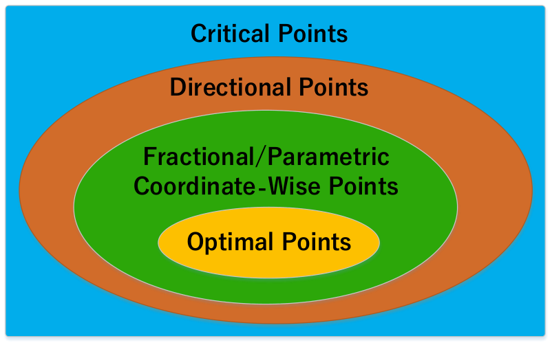
Refer to caption — Figure 3: Left: optimality hierarchy between the optimality conditions. Note that the condition of FCW-point is equivalent to that of PCW-point. Right: Geometric interpretation for the one-dimensional fractional problem with $F(x)\triangleq\frac{(x+2)^{2}}{|3x+2|+1}$ .

$x$	$F(x)$	C-point	D-point	FCW-point	PCW-point
$x_{1}=-\tfrac{2}{3}$	$(\tfrac{4}{3})^{2}$	Yes	No	No	No
$x_{2}=0$	$\frac{4}{3}$	Yes	Yes	No	No
$x_{3}=-2$	0	Yes	Yes	Yes	Yes

Table 3: Points satisfying different optimality conditions.

D.2 A Simple Example for the Optimality Hierarchy

To show the optimality hierarchy between the optimality conditions, we consider the following one-dimensional example which has been mentioned in the paper:

\displaystyle\min_{x}F(\mathbf{x})\triangleq\frac{(x+2)^{2}}{|3x+2|+1}

This problem contains three C-points $\{-\tfrac{2}{3},0,-2\}$ , and we now show that this problem contains one unique Parametric Coordinate-Wise Point (PCW-point). (i) We consider the point $x_{1}=-\frac{2}{3}$ . We have the following parametric problem:

		$\displaystyle~\arg\min_{y}P_{1}(y)\triangleq(y+2)^{2}-F(x_{1})(\|3y+2\|+1)$
	$\displaystyle\overset{(a)}{=}$	$\displaystyle~\arg\min_{y}P_{1}(y)\triangleq(y+2)^{2}-(\tfrac{4}{3})^{2}(\|3y+2\|+1)$
	$\displaystyle\overset{(b)}{=}$	$\displaystyle~\arg\min_{y}P_{1}(y)\triangleq(y+2)^{2}-(\tfrac{4}{3})^{2}(\|3y+2\|+1),s.t.~y\in\{-\tfrac{2}{3},0,-4\}$
	$\displaystyle\overset{(c)}{=}$	$\displaystyle~-4\neq x_{1},$

where step $(a)$ uses $F(x_{1})=(\frac{4}{3})^{2}$ ; step $(b)$ uses the fact that $\{-\tfrac{2}{3},0,-4\}$ are the three critical points of $\min_{y}P_{1}(y)$ ; step $(c)$ uses the fact that $P_{1}(-\tfrac{2}{3})=\frac{4}{9}$ , $P_{1}(0)=0$ , $P_{1}(-4)=-\frac{32}{3}$ , and $y=-4$ is the global minimizer of the problem $\min_{y}P_{1}(y)$ . Since $-4\neq x_{1}=-\frac{2}{3}$ , $x_{1}=-\frac{2}{3}$ is not a PCW-point.

(ii) We consider the point $x_{2}=0$ . We have the following parametric problem:

		$\displaystyle~\arg\min_{y}P_{2}(y)\triangleq(y+2)^{2}-F(x_{2})(\|3y+2\|+1)$
	$\displaystyle\overset{(a)}{=}$	$\displaystyle~\arg\min_{y}P_{1}(y)\triangleq(y+2)^{2}-\tfrac{4}{3}(\|3y+2\|+1)$
	$\displaystyle\overset{(b)}{=}$	$\displaystyle~\arg\min_{y}P_{1}(y)\triangleq(y+2)^{2}-\tfrac{4}{3}(\|3y+2\|+1),s.t.~y\in\{-\tfrac{2}{3},\tfrac{2}{3},-\tfrac{14}{3}\}$
	$\displaystyle\overset{(c)}{=}$	$\displaystyle~-\tfrac{14}{3}\neq x_{2},$

where step $(a)$ uses $F(x_{1})=(\frac{4}{3})^{2}$ ; step $(b)$ uses the fact that $\{-\tfrac{2}{3},\tfrac{2}{3},-\tfrac{14}{3}\}$ are the three critical points of $\min_{y}P_{1}(y)$ ; step $(c)$ uses the fact that $P_{1}(-\tfrac{2}{3})=0$ , $P_{1}(0)=\frac{16}{27}$ , $P_{1}(-4)=-16$ , and $y=-\tfrac{14}{3}$ is the global minimizer of the problem $\min_{y}P_{2}(y)$ . Since $-\tfrac{14}{3}\neq x_{2}=0$ , $x_{2}=0$ is not a PCW-point.

(iii) We consider the point $x_{3}=-2$ . We have the following parametric problem:

		$\displaystyle~\arg\min_{y}P_{3}(y)\triangleq(y+2)^{2}-F(x_{3})(\|3y+2\|+1)$
	$\displaystyle\overset{(a)}{=}$	$\displaystyle~\arg\min_{y}P_{1}(y)\triangleq(y+2)^{2}$
	$\displaystyle\overset{(b)}{=}$	$\displaystyle~-2=x_{3},$

where step $(a)$ uses $F(x_{3})=0$ ; step $(b)$ uses the fact that $y=-2$ is the global minimizer of the problem $\arg\min_{y}P_{1}(y)$ . Since $-2=x_{3}$ , $x_{3}=-2$ is a PCW-point.

Therefore, $x=-2$ is the unique PCW-point.

Figure 3 demonstrates the optimality hierarchy and the geometric interpretation for the one-dimensional problem. Table 3 shows the points satisfying different optimality conditions. We conclude that the condition of FCW-point and PCW-point might be a much stronger condition than the condition of critical point and direction point.

D.3 The Globally or Locally Bounded Non-Convexity Assumption

We prove that $\tilde{g}(\mathbf{x})=-\|\mathbf{G}\mathbf{x}\|_{4}^{2}$ is globally $\rho$ -bounded non-convex, while $\tilde{g}(\mathbf{x})=-\sum_{j=1}^{k}|\mathbf{x}_{[j]}|$ is locally $\rho$ -bounded non-convex.

Lemma D.3.

Assume $\mathbf{x}\neq\mathbf{0}$ and $\mathbf{A}$ has full column rank. The function $\tilde{g}(\mathbf{x})=-\|\mathbf{G}\mathbf{x}\|_{4}^{2}$ is globally $\rho$ -bounded non-convex with $\rho=6m\max_{i}(\mathbf{G}\mathbf{G}^{T})_{ii}\cdot\frac{\lambda_{\max}(\mathbf{G}^{T}\mathbf{G})}{\lambda_{\min}(\mathbf{G}^{T}\mathbf{G})}$ , where $\lambda_{\min}(\mathbf{G}^{T}\mathbf{G})$ and $\lambda_{\max}(\mathbf{G}^{T}\mathbf{G})>0$ denote the smallest and the largest eigenvalue of the matrix $\mathbf{G}^{T}\mathbf{G}$ , respectively.

Proof.

The first-order and second-order gradient of $\tilde{g}(\mathbf{x})$ can be computed as:

	$\displaystyle\nabla\tilde{g}(\mathbf{x})$	$\displaystyle=$	$\displaystyle\frac{2\sum_{i}^{m}(\mathbf{G}_{i}\mathbf{x})^{3}\mathbf{G}_{i}^{T}}{-\\|\mathbf{G}\mathbf{x}\\|_{4}^{2}},$
	$\displaystyle\nabla^{2}\tilde{g}(\mathbf{x})$	$\displaystyle=$	$\displaystyle\frac{6\sum_{i}^{m}[(\mathbf{G}_{i}\mathbf{x})^{2}\mathbf{G}_{i}^{T}\mathbf{G}_{i}]\\|\mathbf{G}\mathbf{x}\\|_{4}^{2}}{-\\|\mathbf{G}\mathbf{x}\\|_{4}^{4}}+\frac{2\sum_{i}^{m}(\mathbf{G}_{i}\mathbf{x})^{3}\mathbf{G}_{i}^{T}\nabla\tilde{g}(\mathbf{x})^{T}}{-\\|\mathbf{G}\mathbf{x}\\|_{4}^{4}},$

where $\mathbf{G}\in\mathbb{R}^{m\times n}$ and $\mathbf{G}_{i}\in\mathbb{R}^{1\times n}$ is the $i$ -the row of $\mathbf{G}$ .

The $\rho$ -bounded nonconvexity of $\tilde{g}(\mathbf{x})$ is equivalent to the convexity of $(\tilde{g}(\mathbf{x})+\tfrac{\rho}{2}\|x\|_{2}^{2})$ . In what follows, we prove that $\nabla^{2}\tilde{g}(\mathbf{x})+\rho\mathbf{I}\succcurlyeq\textbf{0}$ .

(a) We bound the term $\sum_{i}^{m}(\mathbf{G}_{i}\mathbf{x})^{2}\mathbf{G}_{i}^{T}\mathbf{G}_{i}$ . We denote $\mathbf{v}_{i}\triangleq\|\mathbf{G}_{i}\|_{2}^{2}$ with $i=1,2,...,m$ . We have the following upper-bound:

\displaystyle\sum_{i}^{m}(\mathbf{G}_{i}\mathbf{x})^{2}\mathbf{G}_{i}^{T}\mathbf{G}_{i}\preceq\sum_{i}^{m}\|\mathbf{x}\|_{2}^{2}\|\mathbf{G}_{i}\|_{2}^{2}\mathbf{G}_{i}^{T}\mathbf{G}_{i}=\mathbf{G}^{T}diag(\mathbf{v})\mathbf{G}\|\mathbf{x}\|_{2}^{2}\preceq\|\mathbf{G}\|_{2}^{2}\max(v)\|\mathbf{x}\|_{2}^{2},

(62)

where the first inequality uses the Cauchy-Schwarz inequality and the last inequality uses the norm inequality.

(b) We bound the term $\|\mathbf{G}\mathbf{x}\|_{4}^{2}$ . Using the fact that $\sqrt{m}\|\mathbf{y}\|_{4}\geq\|\mathbf{y}\|_{2}\geq\|\mathbf{y}\|_{4}$ for all $\mathbf{y}\in\mathbf{R}^{m}$ . We have the following lower-bound:

\displaystyle\|\mathbf{G}\mathbf{x}\|_{4}^{2}\geq\frac{1}{m}\|\mathbf{G}\mathbf{x}\|_{2}^{2}\geq\frac{1}{m}\lambda_{\min}(\mathbf{G}^{T}\mathbf{G})\|\mathbf{x}\|_{2}^{2}.

(63)

$\displaystyle\nabla^{2}\tilde{g}(\mathbf{x})$	$\displaystyle\overset{(a)}{\succcurlyeq}$	$\displaystyle\frac{6\sum_{i}^{m}[(\mathbf{G}_{i}\mathbf{x})^{2}\mathbf{G}_{i}^{T}\mathbf{G}_{i}]}{-\\|\mathbf{G}\mathbf{x}\\|_{4}^{2}}+\mathbf{0}$
	$\displaystyle\overset{(b)}{\succcurlyeq}$	$\displaystyle-6\frac{\\|\mathbf{G}\\|_{2}^{2}\max(v)\\|\mathbf{x}\\|_{2}^{2}}{\frac{1}{m}\lambda_{\min}(\mathbf{G}^{T}\mathbf{G})\\|\mathbf{x}\\|_{2}^{2}}\cdot\mathbf{I},$
	$\displaystyle\overset{(c)}{=}$	$\displaystyle-6m\max(v)\cdot\frac{\lambda_{\max}(\mathbf{G}^{T}\mathbf{G})}{\lambda_{\min}(\mathbf{G}^{T}\mathbf{G})}\cdot\mathbf{I}=-\rho\mathbf{I},$

where step $(a)$ uses the fact that $\frac{2\sum_{i}^{m}(\mathbf{G}_{i}\mathbf{x})^{3}\mathbf{G}_{i}^{T}\nabla\tilde{g}(\mathbf{x})^{T}}{-\|\mathbf{G}\mathbf{x}\|_{4}^{4}}$ is positive semidefinite, step $(b)$ uses (62) and (63); step $(c)$ uses the definition of $\rho$ .

∎

Note that the assumption $\mathbf{x}\neq\mathbf{0}$ is automatically satisfied by Problem (1) since we assume that $g(\mathbf{x})>0$ .

Lemma D.4.

The function $\tilde{g}(\mathbf{x})=-\sum_{j=1}^{k}|\mathbf{x}_{[j]}|$ is locally $\rho$ -weakly convex with $\rho<+\infty$ .

Proof.

For simplicity, we define $\|\mathbf{x}\|_{[k]}\triangleq\sum_{j=1}^{k}|\mathbf{x}_{[j]}|$ . For any $\mathbf{x}\in\mathbb{R}^{n}$ and a given parameter $k$ , the subgradient of $\|\mathbf{x}\|_{[k]}$ can be computed as $\partial\|\mathbf{x}\|_{[k]}={\{\begin{array}[]{ll}\text{sign}(\mathbf{x}_{i}),&\hbox{ $i\in\Delta_{k}(\mathbf{x})\text{~and~}\mathbf{x}_{i}\neq 0$;}\\ $[-1,1]$,&\hbox{else.}\end{array}\}}$ , where $\Delta_{k}(\mathbf{x})$ is the index of the largest (in magnitude) $k$ elements of $\mathbf{x}$ .

As the two reference points $\mathbf{x}\neq\mathbf{y}$ in Assumption 5.6, we assume that there exists a constant $\epsilon>0$ satisfying $\|\mathbf{x}-\mathbf{y}\|_{2}\geq\epsilon$ . We have:

			$\displaystyle\tilde{g}(\mathbf{x})-\tilde{g}(\mathbf{y})-\langle\mathbf{x}-\mathbf{y},\partial\tilde{g}(\mathbf{x})\rangle$
		$\displaystyle=$	$\displaystyle-\\|\mathbf{x}\\|_{[k]}+\\|\mathbf{y}\\|_{[k]}-\langle\mathbf{x}-\mathbf{y},\partial(-\\|\mathbf{x}\\|_{[k]})\rangle$
		$\displaystyle\overset{(a)}{\leq}$	$\displaystyle\\|\mathbf{y}-\mathbf{x}\\|_{[k]}+\\|\mathbf{y}-\mathbf{x}\\|\cdot\\|\partial(\\|\mathbf{x}\\|_{[k]})\\|$
		$\displaystyle\overset{(b)}{\leq}$	$\displaystyle\\|\mathbf{y}-\mathbf{x}\\|_{1}+\\|\mathbf{y}-\mathbf{x}\\|\cdot\sqrt{n}$
		$\displaystyle\overset{(c)}{\leq}$	$\displaystyle 2\sqrt{n}\\|\mathbf{x}-\mathbf{y}\\|_{2}$
		$\displaystyle\overset{(d)}{\leq}$	$\displaystyle\tfrac{2\sqrt{n}}{\epsilon}\\|\mathbf{x}-\mathbf{y}\\|_{2}^{2},$

where step $(a)$ uses the triangle inequality that $\|\mathbf{y}\|_{[k]}-\|\mathbf{x}\|_{[k]}\leq\|\mathbf{y}-\mathbf{x}\|_{[k]}$ since $\|\cdot\|_{[k]}$ is a norm; step $(b)$ uses the fact that $\|\partial(\|\mathbf{x}\|_{[k]})\|\leq\sqrt{n}$ ; step $(c)$ uses the fact that $\|\mathbf{x}\|\leq\|\mathbf{x}\|_{1}\leq\sqrt{n}\|\mathbf{x}\|$ for all $\mathbf{x}\in\mathbb{R}^{n}$ ; step $(d)$ uses $\|\mathbf{x}-\mathbf{y}\|_{2}\geq\epsilon$ .

Therefore, the function $\tilde{g}(\mathbf{x})$ is $\rho$ -bounded non-convex with $\rho<+\infty$ .

∎

D.4 The function $g(\mathbf{x})=\|\mathbf{G}\mathbf{x}\|_{4}^{2}$ is convex

We prove that the function $g(\mathbf{x})=\|\mathbf{G}\mathbf{x}\|_{4}^{2}$ is convex. We first present the following useful lemma.

Lemma D.5.

Assume that $p(\mathbf{x})$ is a convex and non-negative function. The function $g(\mathbf{x})=(p(\mathbf{x}))^{2}$ is convex.

Proof.

By the convexity of $p(\mathbf{x})$ , we have:

\displaystyle p((1-t)\mathbf{x}+t\mathbf{y})\leq(1-t)p(\mathbf{x})+tp(y),\forall t\in(0,1).

Squaring both sides of the inequality above, we obtain:

			$\displaystyle p((1-t)\mathbf{x}+t\mathbf{y})\cdot p((1-t)\mathbf{x}+t\mathbf{y})$
		$\displaystyle\leq$	$\displaystyle(1-t)(1-t)p(\mathbf{x})p(\mathbf{x})+t^{2}p(y)p(y)+2t(1-t)p(\mathbf{x})p(\mathbf{y})$
		$\displaystyle=$	$\displaystyle(1-t)p(\mathbf{x})p(\mathbf{x})-(1-t)tp(\mathbf{x})p(\mathbf{x})+t^{2}p(y)p(y)+2t(1-t)p(\mathbf{x})p(\mathbf{y})$
		$\displaystyle=$	$\displaystyle(1-t)p(\mathbf{x})p(\mathbf{x})+tp(y)p(y)-t(1-t)(p(y)-p(\mathbf{x}))^{2}$
		$\displaystyle\leq$	$\displaystyle(1-t)p(\mathbf{x})p(\mathbf{x})+tp(y)p(y).$

where the last step uses $t\in(0,1)$ and $(p(y)-p(\mathbf{x}))^{2}\geq 0$ .

∎

Note that $p(\mathbf{x})=\|\mathbf{G}\mathbf{x}\|_{4}$ is a convex and non-negative function. Using Lemma D.5, we conclude that $g(\mathbf{x})=\|\mathbf{G}\mathbf{x}\|_{4}^{2}$ is convex with respect to $\mathbf{x}$ .

	$\displaystyle\frac{1}{n}\sum_{i=1}^{n}\\|\mathbf{x}+\mathbf{d}_{i}e_{i}\\|_{2}^{2}$	$\displaystyle=$	$\displaystyle\frac{1}{n}\\|\mathbf{d}\\|_{2}^{2}+\frac{2}{n}\langle\mathbf{x},\mathbf{d}\rangle+\\|\mathbf{x}\\|_{2}^{2}$
		$\displaystyle=$	$\displaystyle\frac{1}{n}\\|\mathbf{d}+\mathbf{x}\\|_{2}^{2}+(1-\frac{1}{n})\\|\mathbf{x}\\|_{2}^{2}$

Abstract

1 Introduction

2 Applications

3 Related Work

4 Proposed Coordinate Descent Methods

5 Theoretical Analysis

5.1 Technical Preliminaries

Definition 5.1.

Definition 5.2.

Assumption 5.3.

Lemma 5.4.

Lemma 5.5.

5.2 Convex-Convex FMPs

Definition 5.6.

5.2.1 Optimality Analysis

Definition 5.7.

Definition 5.8.

Lemma 5.9.

Theorem 5.10.

5.2.2 Convergence Analysis

Definition 5.11.

Proposition 5.12.

Assumption 5.13.

Theorem 5.14.

Theorem 5.15.

5.3 Convex-Concave FMPs

Proposition 5.16.

Theorem 5.17.

6 Implementations and Experiments

6.1 Implementations for Sparse Recovery

6.2 Implementations for ℓp\ell_{p} Norm Eigenvalue Problem

6.3 Experiment Settings

6.4 Experiment Results

References

Appendix A Proofs for Section 5.1

A.1 Proof of Lemma 5.4

Proof.

A.2 Proof of Lemma 5.5

Proof.

A.3 Proof of Lemma 5.9

Proof.

Appendix B Proofs for Section 5.2

B.1 Proof of Theorem 5.10

Proof.

B.2 Proof of Proposition 5.12

Proof.

B.3 Proof of Theorem 5.14

Proof.

B.4 Proof of Theorem 5.15

Proof.

Appendix C Proofs for Section 5.3

C.1 Proof of Proposition 5.16

Proof.

C.2 Proof of Theorem 5.17

Proof.

Appendix D Additional Discussions

D.1 Fractional Reformulations for Problem (4)

Proposition D.1.

Proof.

Proposition D.2.

Proof.

D.2 A Simple Example for the Optimality Hierarchy

D.3 The Globally or Locally Bounded Non-Convexity Assumption

Lemma D.3.

Proof.

Lemma D.4.

Proof.

D.4 The function g⁡(𝐱)=‖𝐆𝐱‖42g(\mathbf{x})=\|\mathbf{G}\mathbf{x}\|_{4}^{2} is convex

Lemma D.5.

Proof.

6.2 Implementations for $\ell_{p}$ Norm Eigenvalue Problem

D.4 The function $g(\mathbf{x})=\|\mathbf{G}\mathbf{x}\|_{4}^{2}$ is convex