An Indirect Rate-Distortion Characterization for Semantic Sources: General Model and the Case of Gaussian Observation
Abstract
A new source model, which consists of an intrinsic state part and an extrinsic observation part, is proposed and its information-theoretic characterization, namely its rate-distortion function, is defined and analyzed. Such a source model is motivated by the recent surge of interest in the semantic aspect of information: the intrinsic state corresponds to the semantic feature of the source, which in general is not observable but can only be inferred from the extrinsic observation. There are two distortion measures, one between the intrinsic state and its reproduction, and the other between the extrinsic observation and its reproduction. Under a given code rate, the tradeoff between these two distortion measures is characterized by the rate-distortion function, which is solved via the indirect rate-distortion theory and is termed as the semantic rate-distortion function of the source. As an application of the general model and its analysis, the case of Gaussian extrinsic observation is studied, assuming a linear relationship between the intrinsic state and the extrinsic observation, under a quadratic distortion structure. The semantic rate-distortion function is shown to be the solution of a convex programming problem with respect to an error covariance matrix, and a reverse water-filling type of solution is provided when the model further satisfies a diagonalizability condition.
I Introduction
A standard approach to describe an information source is to model a source as a stochastic process , and when the stochastic process is memoryless, it suffices to model a source as a random variable11 1 In this paper, random variables can be drawn from general alphabets, so random vectors are vector-valued random variables. with a given probability distribution [2] [3]. In this paper, we study a new source model, which consists of an intrinsic state process and an extrinsic observation process. In the memoryless case, we can describe such a source model as a pair of random variables , with a given joint probability distribution , defined over an appropriate product alphabet .
In order to characterize the information-theoretic aspect of such a source, consider the problem of compressing the source so as to reproduce, in a lossy sense, a reproduction over a reproduction product alphabet . Of course, a pair of distortion measures, and , are introduced correspondingly. Here, the subscript stands for “state” and the subscript stands for “observation”. A key point of the problem is that the compressor only has access to , the extrinsic observation; — while , the intrinsic state, remains unrevealed. The situation is illustrated in Figure 1.
Our source model, termed as a semantic source in the sequel, is motivated by the recent surge of interest in the semantic aspect of information. In a number of applications that may benefit from taking into account the “semantic” feature of information, it is adequate to adopt a goal-oriented perspective; that is, the destination’s interest in obtaining a piece of information is to accomplish a certain goal. Furthermore, it is customary to adopt an inference-theoretic problem formulation, which casts the accomplishment of the said goal as solving a statistical inference problem. The reproduction of the intrinsic state corresponds to the semantic inference part of the source, and the reproduction of the extrinsic observation corresponds to the conventional lossy compression part of the source.
We give two examples of the above consideration:
- •
Systems that support MPEG Video Coding for Machines (VCM) are becoming popular in applications. In VCM, both the video itself and its features are reproduced: the video signal is for human vision, and the features are for machine vision tasks [4] [5] [6]. Treating the video as a semantic source, the video signal itself corresponds to its extrinsic observation, and the underlying features correspond to its intrinsic state, so as to embody the semantic aspect of the video. Usually the code rate required for reproducing features can be drastically lower than that required for reproducing the video signal itself. Intuitively, features typically have much smaller rate distortion functions and hence can be described with many fewer bits, compared with video signals. For instance, previous works have shown that neural network-based learning techniques can extract a very small amount of data from video signals to satisfy the need of action recognition, target classification and many other tasks [7] [8]. In contrast, traditional video coding schemes such as H.264/AVC/MPEG-4 and H.265/HEVC/MPEG-H Part 2 only target at reproducing the video signal with high fidelity, but may perform poorly for machine vision purposes [9].
- •
In coding of speech signals, the semantic aspect is embodied as a sequence of text words, which, of course, can only be inferred from the speech signal itself. Treating the speech as a semantic source, the words correspond to its intrinsic state and the speech signal corresponds to its extrinsic observation. It is the usual case that both the words and the speech signal are desirable, because the words carry the meaning of speech, and the speech signal waveform may help us infer the stress and emotion of the speaker [10], and may further help us accomplish tasks like speaker recognition and speaker verification [11].
Our main contributions include:
- •
We propose a theoretical framework based on rate distortion theory for characterizing semantic information.
- •
We define and derive a single-letter expression for the semantic rate distortion function.
- •
When the extrinsic observation is Gaussian and satisfies a linear relationship with the intrinsic state, we reduce the calculation of the semantic rate distortion function to a convex programming problem, which is tractable with standard scientific computing software. Furthermore, under a diagonalizability condition, we obtain a weighted reverse water-filling solution for the semantic rate distortion function.
We give a brief overview of related works in the remaining part of this section. Then we provide a formal mathematical description of the semantic source model and the corresponding semantic rate-distortion problem formulation in Section II, for which we establish the semantic rate-distortion function in general form in Section III. As an application of the general results, in Section IV we turn to a case study of Gaussian extrinsic observation, assuming a linear relationship between the intrinsic state and the extrinsic observation, under a quadratic distortion structure. Therein, we formulate a convex programming to solve the semantic rate-distortion function. When the Gaussian observation model further satisfies a diagonalizability condition, we develop a reverse water-filling type of solution in Section V. Finally we conclude this paper in Section VI.
I-A Related Works
The first formulation in Shannon’s information theory is lossless source coding, wherein a sequence of symbols obeying a certain probabilistic law is represented as a bit string (i.e., a codeword) by an encoder, and the decoder reproduces, based upon the codeword, the original sequence of symbols, with success probability exactly one or asymptotically approaching one. Hence, the coding is solely determined by the probabilistic model of the source, and there is certainly no role of the semantic aspect of the source. This is also consistent with Shannon’s remark in his landmark paper [2], saying “these semantic aspects of communication are irrelevant to the engineering problem.”
In a broad sense, however, the lossy source coding formulation in Shannon’s information theory, namely, the rate-distortion theory [12], has provided a means of studying the semantic aspects of a source. This is because the coding is not solely determined by the probabilistic model of a source, but is also affected by a distortion measure, which may be defined in a rather versatile way so as to capture the “utility” when the source is reproduced at the decoder.
Our present work goes one step further, by endowing a source with a state-observation structure and studying the rate distortion function of such a source model. This model captures the fact that the semantic aspects of a source are generally embedded as intrinsic features, and hence should be characterized by studying the reproduction of the intrinsic state, in addition to the reproduction of the extrinsic observation. Our treatment of semantic aspects of sources is also in line with the recently heightened interest in the development of 5G and beyond wireless systems [13] [14] [15], where for many applications the semantic aspects correspond to the accomplishment of certain inference goals. Hence, if we consider an information theoretic characterization of such a “semantic” source, the task of coding is to efficiently encode the extrinsic observation so that the decoder can infer both the intrinsic state and the extrinsic observation, subject to fidelity criteria on both, simultaneously. Our problem formulation and approach are closely related to two variants of the standard rate distortion theory, namely, indirect rate distortion function and rate distortion function under multiple distortion measures; see our discussion following Theorem 1 in Section III.
The inference-theoretic goal-oriented approach adopted in our problem formulation does not seek a task-independent universal definition of semantic information, which is outside the scope of the present paper; for some attempts in that regard, see, e.g., [16] [17] [18] [19] for a few representative works that undertake drastically different approaches.
As related topics, the information bottleneck [20] [21] and the privacy funnel [22] [23] are, in a certain sense, dual concepts, and both place constraints in terms of mutual information. The underlying idea of the information bottleneck is, in a broad sense, similar to ours. Specifically, there one generates a reproduction based upon the extrinsic observation, minimizing the mutual information between the extrinsic observation and the reproduction, while maintaining a level of mutual information between the intrinsic state and the reproduction. But for the information bottleneck problem formulation, there is neither explicit distortion measure, nor operational definition of lossy compression.
Task-based compression has been approached mainly from the perspective of quantizer design [24]. It has been demonstrated that steering the design goal according to the task leads to performance benefits compared with conventional task-agnostic approach, a conclusion in line with what we advocate in our work. The perception-distortion tradeoff [25] imposes an additional constraint on the probability distribution of the reproduction. None of these related works proposes to decompose the information source into intrinsic and extrinsic parts as in our work, let alone investigate the joint behavior of them. In [26], a similar intrinsic state-extrinsic observation model is studied, but the encoder is designed based on the marginal distribution of the extrinsic observation only.
II System Model and Problem Formulation
As already outlined in the introduction, we model a memoryless semantic source as a pair of random variables that are correlated with joint probability distribution . The semantic aspect is embodied in the intrinsic state , which is not observable but can only be inferred from the extrinsic observation . In order to characterize the rate-distortion behavior of the semantic source, we consider a sequence of independent and identically distributed (i.i.d.) samples of , denoted as , and denote its length- block as .
The i.i.d. source model is an idealistic scenario for our information-theoretic study. Real-world data generally exhibit sophisticated memory structures. A particularly interesting scenario is when the intrinsic state is a Markov chain, and the extrinsic observation obeys a hidden Markov model (HMM) [27]. Extensions of our approach for semantic source models with memory are left for future research.
The lossy compression of a semantic source has been illustrated in Figure 1. The encoder only has access to a length- block of the extrinsic observation sequence , and the decoder has two tasks: reproducing the intrinsic state block as under a state distortion measure , and reproducing the extrinsic observation block as under an observation distortion measure . The encoder and the decoder are connected via a bit pipe in which the codeword of bits is transferred from the encoder to the decoder, where is thus the code rate of the lossy compression system.
Below we provide a formal description of the lossy compression problem of a semantic source.
Let and be two given distortion measures, defined over the source product alphabet and the reproduction product alphabet . The extended block-wise distortion measures are as follows:
| (1) | ||||
| (2) |
We claim a tuple to be achievable, if for any and all sufficiently large , there exist the following functions:
- •
Encoding function which generates the codeword as ;
- •
State decoding function , such that
(3) where ;
- •
Observation decoding function , such that
(4) where .
It is clear that the state decoding function and the observation decoding function together constitute the decoder illustrated in Figure 1.
Our goal is to characterize the region of all achievable tuples. Hence, we define the semantic rate distortion function as follows22 2 This is the operational definition of a rate distortion function, which has been widely used (see, for example, [3] [28] [29]).:
| (5) |
Clearly, characterizing the semantic rate distortion function is equivalent to characterizing the achievable region of .
We will also consider a variant of the distortion constraint; that is, the state distortion and the observation distortion are linearly combined to yield a single overall distortion. Hence, instead of (3) and (4), the decoding functions are required to satisfy the following weighted distortion constraint:
| (6) |
where and are non-negative weighting coefficients.
It is also natural to generalize the system model to include several intrinsic state variables each associated with a specified reproduction and a distortion. Such a semantic source is described by a tuple of random variables, , with joint probability distribution over , where each is an intrinsic state reflecting a certain semantic aspect of the source. The decoder now consists of an observation decoding function and state decoding functions, among which maps the codeword into a reproduction sequence to satisfy
| (7) |
The notion of achievability can be defined in a similar fashion with respect to the tuple , , , , , , and the semantic rate distortion function is consequently defined as
| (8) |
III Semantic Rate Distortion Function
In this section, we establish in the following theorem a single-letter characterization of the semantic rate distortion function defined in Section II.
Theorem 1
For a given semantic source with over , reproduction alphabet , and distortion measures and , the semantic rate distortion function is as follows:
| (9) | ||||
| s.t. | (10) | |||
| (11) |
where
| (12) |
and constitute a Markov chain .
Proof: See Appendix A.
Here we briefly discuss the basic idea of the proof of Theorem 1. There are two main ingredients in the problem formulation: an indirect rate distortion problem which has been studied in [30] [31] [32, Chap. 3, Sec. 5] [33], and a rate distortion problem with several distortion constraints which has been studied in [34, Sec. VII] [3, Prob. 10.19] [35, Prob. 7.14]. A key is to recognize reproducing as an indirect rate distortion problem, for which the state distortion between and can be equivalently converted to a distortion between and . Indeed, the converted distortion is nothing but the conditional expectation of the original state distortion , over . This conversion hence circumvents the difficulty due to the absence of access to at the encoder. The detailed derivation, which is based on a unified treatment in [33], is given in Appendix A.
We note that the semantic rate distortion function can be non-trivial even for the special case where is a deterministic function of , because from a lossy reproduction of it is generally impossible to reproduce in a lossless fashion. Specifically, suppose that . Then can be simplified into
| (13) |
Similar to standard rate distortion functions, a corollary of the semantic rate distortion function as given by Theorem 1 is the following regarding monotonicity and convexity.
Corollary 1
The semantic rate distortion function in Theorem 1 has the following properties:
- •
is monotonically nonincreasing with and .
- •
is jointly convex with respect to .
- •
The contour set is convex for any .
Proof: The proof of the first two properties is exactly the same as that for standard rate distortion functions; see, e.g., [3]. The third property is then an immediate corollary of the second property.
Corollary 1 implies a trade-off between the two distortions: for a given code rate, the smaller the state distortion, the larger the observation distortion, and vice versa. Concrete numerical examples can be found in Section IV, where Figures 2 and 4 plot the achievable regions of and their projections under different values of , for two experimental setups, respectively. These plots demonstrate that for fixed , the achievable pairs form a convex region, whose boundary exhibits a trade-off between and . Hence a sensible coding scheme of a semantic source should exhibit such behavior.
Now consider the weighted distortion constraint (6). We have the following corollary.
Corollary 2
For a given semantic source under the weighted distortion constraint (6), the rate distortion function is as follows:
| (14) |
Proof: Given the semantic rate distortion function in Theorem 1, we have that any coding scheme that achieves should achieve a tuple for the semantic rate distortion problem under distortion constraints (3) and (4), for some and satisfying , and vice versa.
We end this section with the semantic rate distortion function (8) for semantic sources with several intrinsic states, as given by the following corollary. Its proof is essentially identical to that of Theorem 1.
Corollary 3
For a semantic source with over , reproduction alphabet , and distortion measures and , the semantic rate distortion function is as follows:
| (15) | ||||
| s.t. | (16) | |||
| (17) |
where
| (18) |
and constitute a Markov chain .
IV Gaussian Observation with Linear State-Observation Relationship
Theorem 1 establishes the general form of the semantic rate distortion function, which comes with an optimization problem, extending its counterpart in a standard rate distortion problem. In this section, we specialize the general result to a case where the extrinsic observation is Gaussian and the intrinsic state-extrinsic observation pair satisfies a linear relationship, under quadratic distortion measures.
The extrinsic observation obeys a multivariate Gaussian distribution ,33 3 We use to denote the covariance matrix of a random column vector . where is an positive semi-definite matrix. The intrinsic state is given by
| (19) |
where is an matrix, and is a random vector independent of , with zero mean and covariance matrix . Note that we neither restrict to be Gaussian nor require or to be full-rank. According to (19), the intrinsic state is a linear transformation of , further disturbed by an independent component . This linear assumption holds for jointly Gaussian intrinsic state and extrinsic observation , and can usually be extended to non-Gaussian models as well, either precisely or approximately, for example, when a linear estimator of conditioned upon can be obtained by traditional statistical methods, or by multilayer perceptron (MLP) neural networks alternatively [36]. On the other hand, note that the linear assumption no longer holds when one invokes nonlinear mappings, and deriving an analytical form of the corresponding semantic rate distortion function will generally be an extremely difficult task.
This model covers the special case where are jointly Gaussian. In fact, if are jointly Gaussian with zero mean and covariance matrix
| (20) |
we can represent according to
| (21) |
where ; that is, and .
We consider quadratic distortion measures, defined as
| (22) | ||||
| (23) |
Consequently, we have
| (24) | ||||
| (25) |
For the considered model (19), we can derive its semantic rate distortion function, given by the following theorem.
Theorem 2
The semantic rate distortion function for the semantic source with Gaussian extrinsic observation and linear state-observation relationship (19), under quadratic distortion measures (22) and (23), is given by:
| (26) | ||||
| s.t. | (27) | |||
| (28) | ||||
| (29) |
where denotes the set of all positive definite matrices. Note that here we use a subscript to emphasize that the extrinsic observation is Gaussian.
Proof: See Appendix B.
From (28), when is sufficiently strong so that , the optimization (26) is no longer feasible and hence . Otherwise, there is no further restriction on . For example, even if , i.e., the relationship between and is deterministic as , the optimization problem in Theorem 2 is still non-trivial.
A simplified case arises when is an orthogonal matrix satisfying . In this case, (28) becomes
| (30) |
which can then be combined with (29) leading to a single distortion constraint
| (31) |
In Theorem 2, the matrix which we optimize corresponds to the mean squared error (MSE) of estimating based upon at the decoder. The key to the proof of Theorem 2 is to show that the semantic rate distortion function is achieved by a Gaussian reproduction. This is similar to situations in several Gaussian lossy compression problems, including the standard Gaussian rate distortion problem [12] and the Gaussian quadratic CEO problem [37]. Existing techniques based on the entropy power inequality (EPI), extremal inequalities, and Fisher information inequalities may also be interpreted as the optimality of Gaussian reproduction for the minimum mean squared error (MMSE) estimation under a given MSE constraint. In our analysis, we further need to accommodate with two MSE constraints, corresponding to the intrinsic state and the extrinsic observation, respectively.
Compared with the general form of semantic rate distortion function in Theorem 1, Theorem 2 involves only one matrix-valued optimization variable , which, as remarked in the previous paragraph, is the MSE of estimating based upon alone. In fact, the solution exhibits a Markov structure, i.e., . To help understand the optimality of the Markov chain solution, supposing that an alternative solution is given which does not satisfy the Markov structure, consequently one can form an improved reproduction as , satisfying the Markov structure and achieving the same code rate .
The Markov chain solution further suggests a “two-stage” coding interpretation which is in fact extensively adopted in practice: the decoder first generates a reproduction for as , and then uses that reproduction to further generate a reproduction for as . Similar to the standard Gaussian rate distortion problem, the optimal can be constructed with the aid of a “test channel”, for which as the channel input is Gaussian and the additive Gaussian noise of the test channel has a covariance matrix , thereby producing as the desired channel output. To generate based upon , it suffices to adopt a linear transform . On the other hand, the Markov chain solution does not mean that the reproduction of is trivial, because the fidelity criterion on still needs to be adjusted according to . The detailed arguments are given in the proof in Appendix B.
An interesting property of the semantic rate distortion function derived in Theorem 2 is that it is in fact an upper bound for all semantic sources with the same covariance structure under the quadratic distortion measure. This essentially indicates that a semantic source with Gaussian extrinsic observation is the hardest to describe, analogous to its counterpart in conventional source coding problems (see, e.g., [3, Exercise 10.8]). Formally, we have the following corollary.
Corollary 4
Proof: See Appendix C.
IV-A Computation of the Semantic Rate Distortion Function
We remark that the optimization problem in Theorem 2 is convex, and hence can be numerically solved by software like CVX in an efficient and stable fashion. In this subsection we present some illustrative numerical examples.
Our first example is a small-scale toy model, given by
The resulting semantic rate distortion function is computed as displayed in Figure 2. The dotted region in Figure 2(b) indicates that both constraints (28) and (29) are active. The trade-off between the two distortions are clear: the smaller the state distortion, the larger the observation distortion, and vice versa.


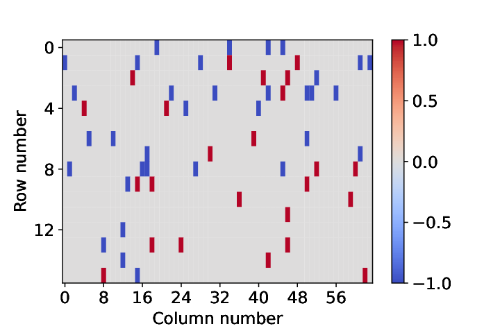
Our second example captures a sparse state-observation relationship, as follows. The extrinsic observation is a length-64 vector consisting of i.i.d. random variables. The transformation matrix is a randomly masked Rademacher matrix; that is, we first generate a Rademacher matrix whose elements are i.i.d. taking values with equal probability , and then independently reset these elements to zero with probability . A realization of is shown in Figure 3. The noise vector consists of i.i.d. random variables.
We numerically solve the semantic rate distortion function according to Theorem 2, and a typical surface of is illustrated in Figure 4(a). More details of can be seen from the contour plot in Figure 4(b), wherein the dotted region indicate that both constraints (28) and (29) are active. From Figure 4(b), it is evident that describing the extrinsic observation tends to be much more costly than describing the intrinsic state : at the same code rate, the achieved is generally much lower than the achieved .


Another interesting fact regarding can be inferred from the dotted region in the contour plot Figure 4(b), and is more clearly revealed by plotting the trends of as a function of (for fixed ) or (for fixed ), shown in Figures 5(a) and 5(b), respectively. We find that, the code rate as a function of does not seem to be sensitive to the choice of . This fact has an important consequence for designing lossy compression schemes for semantic sources: although several different codes may have similar performance in terms of reproducing the extrinsic observation, they can differ considerably in terms of reproducing the intrinsic state. A heuristic explanation is as follows: since is a high-dimensional vector, describing it along several different directions may lead to similar quadratic distortion performance; but since corresponds to a low-dimensional feature of , its reproduction only favors the direction of describing that retains the feature of the best.


IV-B Generalizations of Theorem 2
We can derive from Theorem 2 several corollaries corresponding to the variants of the problem formulation in Section II.
First, let us consider replacing the quadratic distortion measures by the positive semi-definite distortion constraints. Following the same arguments in the proof of Theorem 2, we again arrive at the optimality of Gaussian descriptions under positive semi-definite distortion constraints, and hence the following corollary characterizes the semantic rate distortion function.
Corollary 5
Consider the positive semi-definite distortion measures as
The semantic rate distortion function is given by
| (32) | ||||
| s.t. | (33) | |||
| (34) | ||||
| (35) |
This is a semi-definite programming problem and can be readily solved by software.
Now consider the weighted distortion constraint, where the distortion measure is defined as a weighted sum of two individual distortion measures, i.e.
| (36) |
Applying Corollary 2, we obtain the semantic rate distortion function in the following corollary.
Corollary 6
For the weighted distortion measure , the semantic rate distortion function is given by
| (37) | ||||
| s.t. | (38) | |||
| (39) |
Finally, consider the case of intrinsic states. The extrinsic observation is still . For each , the -th intrinsic state is generated according to
where is an matrix, and is a random vector independent of , with zero mean and covariance matrix . We consider quadratic distortion measures, as
| (40) | ||||
| (41) |
The semantic rate distortion function is given by the following corollary.
Corollary 7
For the semantic source with a Gaussian extrinsic observation and intrinsic states, the semantic rate distortion function under distortion measures , , , , is
| s.t. | |||
V Weighted Reverse Water-Filling
Analogous to the standard Gaussian rate distortion problem wherein (after appropriate linear transformation) the solution can be interpreted as a reverse water-filling type of rate allocation, for the semantic rate distortion function in Theorem 2, under a diagonalizability condition, the solution can also be interpreted as reverse water-filling, but with appropriately weighted water levels.
For the model of Gaussian observation with linear state-observation relationship in Section IV, we further assume that the following diagonalizability condition is satisfied: there exists an unitary matrix such that
- •
,
- •
simultaneously hold. Here it loses no generality to order so that . Denoting the rank of as , then and .
Lemma 1
Under the diagonalizability condition, the resulting optimal takes the form
| (42) |
and the semantic rate distortion function in Theorem 2 can be further written in terms of the following optimization problem:
| (43) | ||||
| s.t. | (44) | |||
| (45) | ||||
| (46) |
Proof: See Appendix D.
In order to describe the weighted reverse water-filling solution, we first introduce the following curves.
- •
Curve :
(47) which starts from and ends at .
- •
Curve :
(48) which starts from and ends at . Here, is interpreted as 0 if is full-rank and thus .
We then introduce the following partitioning of the plane, based upon the curves and :
- •
;
- •
: on the right of the curve , and between the two horizontal lines and ;
- •
: above the curve , and between the two vertical lines and ;
- •
: surrounded by the curves and , and the vertical line .
An example of the partitioning above is plotted in Figure 7.
The following theorem describes the weighted reverse water-filling solution.
Theorem 3
For the model of Gaussian observation with linear state-observation relationship in Section IV, under the diagonalizability condition, the optimal is given by
- •
If :
(49) - •
If :
(50) where is chosen to satisfy .
- •
If :
(51) where is chosen to satisfy .
- •
If :
(52) where , are chosen to satisfy and .
Proof: See Appendix D.
The partitioning is closely related to activity of the constraints (45) and (46), as summarized in Table I. In , both constraints are inactive, and hence the optimization is unconstrained yielding the trivial solution (49). In , only the observation distortion constraint is active, and the solution (50) is a standard reverse water-filling with water level . In , only the state distortion is active, and the solution (51) essentially makes the weighted eigenvalues , , , fulfill a reverse water-filling structure, with water level . Alternatively, we may view the term in (51) as a water level with weight . In , both constraints are active, and the solution (52) also fulfills a reverse water-filling structure with unequal water levels.
| (45) active | (45) inactive | |
|---|---|---|
| (46) inactive | ||
| (46) active |
V-A Case Study: Circulant and and Weighted Reverse Water-filling in Frequency Domain
A case of special interest is where and are both circulant matrices [38]. As the dimension of grows large, this models the scenario where is a circularly stationary Gaussian process,44 4 If we remove the circulant restriction and consider a stationary Gaussian process, then we encounter a Toeplitz , for which our solution still approximately applies; see, e.g., [38]. and is obtained via passing through a time-invariant linear filter whose response is given by the first row of . For a circulant matrix, the corresponding unitary matrix is the well known discrete Fourier transform (DFT) matrix, and its eigenvalues are the DFT of the first row of the matrix. Hence the weighted reverse water-filling may be interpreted as exercised in the frequency domain, similar to its counterpart for the standard rate distortion function of stationary Gaussian processes.
In the illustrative example below, consider as a circulant matrix with the first row
as a circulant matrix with the first row
and as a zero matrix (i.e., no noise in the state-observation relationship). Therefore, is the DFT matrix whose -th element is
The diagonal elements , , , of are shown in Figure 7, and the diagonal elements , , , of are shown as the blue solid curve in Figure 8. Figure 7 shows the four regions , , , and the two curves , . It also displays five points on the contour of , marked with colors varying from purple to yellow. The weighted reverse water-filling solution for these points are depicted in Figure 8. For , the optimal solution degenerates into a standard reverse water-filling form, as indicated by the purple line. When we go from to , the water level begins to “ripple”. Note that this weighted reverse water-filling can be viewed as exercised in the frequency domain, and the angular frequencies are marked on the top of Figure 8.


VI Conclusion
We have provided a general source model to describe information sources that have semantic aspects, and proposed a corresponding rate distortion problem formulation for characterizing the amount of information content of such semantic sources. We have studied the case of Gaussian extrinsic observation subject to a linear state-observation relationship and a quadratic distortion structure. There are a variety of issues that we have not touched upon in the present work. First, calculating and bounding the semantic rate distortion functions for other interesting cases would make further use of our proposed framework, for example, when the intrinsic state is a discrete categorical random variable, corresponding to the important problem of classification; see [1] for some preliminary results. Second, a more challenging problem is to estimate the semantic rate distortion function, and more importantly, to develop effective lossy compression methods when the joint probability distribution of the intrinsic state and the extrinsic observation is not perfectly known, say, when only finite training data of the state-observation pair are available.
Appendix A Proof of Theorem 1
The key to proving Theorem 1 is converting the semantic rate distortion problem into an equivalent standard rate distortion problem, with an indirect (state) distortion constraint and a direct (observation) distortion constraint. More precisely, we need to show that the constraint with respect to the state distortion measure is equivalent to a constraint on a converted distortion measure ; that is, as long as a reproduction satisfies the constraint on , it will satisfy the constraint on , and vice versa.
A general and unified approach to the indirect rate-distortion function put forward in [33] is first showing that the one-shot expected distortion is equivalent to , and then invoking a tensorization argument to extend the one-shot equivalence to block codes. Here we directly illustrate how this can be accomplished for generated by an arbitrary encoder-decoder pair, as follows:
| (53) | |||||
where , , is due to the existence of the Markov chain and hence , follows from the definition of block-wise distortion measure in (1), is by the fact that is an i.i.d. sequence, and is by the definition of in (12). Subsequently, the problem is reduced into a standard lossy source coding problem with two distortion constraints, one on and the other on . The semantic rate distortion function hence follows from standard achievability and converse proofs [34, Sec. VII] [35, Prob. 7.14] [3, Prob. 10.19].
Appendix B Proof of Theorem 2
The proof of Theorem 2 involves two steps. First we prove that the semantic rate distortion function can be achieved by jointly Gaussian and . Then we show that we can further endow a Markov chain structure on , and , so that we only need to optimize with one variable, i.e., , while generating from subsequently.
B-A Optimality of Jointly Gaussian Reproduction
By the definition of in (12), can be written as follows:
| (54) |
where is due to independence between and , is according to the problem setup that , and is due to the fact that . From this chain of identities, we see that for any two reproductions of the intrinsic state, and , we have as long as and .
Therefore, by Theorem 1, the semantic rate distortion function can be further written as
| (55) | ||||
| s.t. | (56) | |||
| (57) |
Notice that, by denoting for convenience, can be upper bounded as
| (58) |
where is by the fact that conditioning reduces entropy, and equality holds when is independent of ; is due to the fact that Gaussian distribution maximizes differential entropy with given second central moment. Overall, we can see that this upper bound of is achieved when and are jointly Gaussian.
Based on the argument above, for an arbitrary , we can generate according to a linear relationship
| (59) |
where is a multivariate Gaussian random variable following and is independent of . Clearly it holds that and . According to (58), we can see that . That is to say, for any that satisfies the distortion constraints, there always exists a Gaussian which also satisfies the distortion constraints, but achieving a lower code rate. We thus establish that jointly Gaussian reproduction achieves the semantic rate distortion function.
B-B Reduction to One Optimization Variable
In fact, it is unnecessary to optimize with two random variables simultaneously, and in the following we reduce the number of optimization variables to only one. We choose the new optimization variable as , defined as
i.e., the error covariance matrix of MMSE estimating by . By denoting as for short, we can write as (26). Therefore, now the key point is to show that the feasible region defined by (56)-(57) (denoted as ) is the same as the feasible region defined by (27)-(29) (denoted as ).
First we show that . For any , with , we have and , and correspondingly and
| (60) |
That is to say, for any , we can find a corresponding , and hence .
Then we show that . For any , we consider a test channel with and let , where obeys Gaussian distribution . Hence we have
| (61) | ||||
| (62) |
That is to say, for any , we can also find a corresponding tuple of , and hence .
Appendix C Proof of Corollary 4
By Theorem 2 and the identities and in (21), the semantic rate distortion function of a jointly Gaussian semantic source with covariance matrix (20) is given by
| (63) | ||||
| s.t. | (64) | |||
| (65) | ||||
| (66) |
We will prove
| (67) |
for an arbitrary symmetric matrix that satisfies (64), (65) and (66), by constructing a test channel. This implies that is no greater than (63).
In order to construct the test channel, let be a Gaussian vector with zero mean and covariance matrix , independent of . That is semi-definite will be proved in Lemma 2 at the end of this subsection. Define and . Thus is a Markov chain. We will verify in the next paragraphs that , where , , and
| (68) |
By the definitions of and , we have , where . Noticing and , we can obtain, after some algebraic manipulations,
Taking the trace in this equation and using (65), we get . Similar calculations lead to . For every and every , we have
where the second equality is due to . An application of the law of total expectation immediately leads to .
It remains to verify (68). We have
where (a) is by , (b) is because after translation , and (c) is because the Gaussian distribution maximizes the differential entropy subject to a covariance constraint.
Finally let us verify the existence of the auxiliary random vector .
Lemma 2
For any , , , is semi-definite.
Proof: Because is positive definite, there exists an matrix such that . For every ,
because is negative definite. So does not have any negative eigenvalue. Therefore is positive semi-definite, and consequently is also positive semi-definite.
Appendix D Derivation of the Weighted Reverse Water-Filling Solution
We first rewrite (26) with a variable substitution . This leads to
where is the set of positive definite real matrices that satisfy
Any optimal in this minimization is diagonal. To see this, consider a non-diagonal . Replacing the non-diagonal elements in with zeros, we get a new matrix . Because
we have for each , which impies . Moreover,
So . By Hadamard’s inequality,
Therefore, any non-diagonal is suboptimal, and (43) is verified.
By the Karush-Kuhn-Tucker (KKT) optimality conditions, there exist non-negative numbers , , , , , that satisfy
References
- [1] J. Liu, W. Zhang, and H. V. Poor, “A rate-distortion framework for characterizing semantic information,” Proc. IEEE Int. Symp. Inf. Theory (ISIT), 2021.
- [2] C. E. Shannon, “A mathematical theory of communication,” Bell Syst. Tech. J., vol. 27, no. 3, pp. 379–423, 1948.
- [3] T. M. Cover and J. A. Thomas, Elements of Information Theory, 2nd ed. Hoboken, New Jersey, USA: John Wiley & Sons, Ltd, 2006.
- [4] S. Ma, X. Zhang, S. Wang, X. Zhang, C. Jia, and S. Wang, “Joint feature and texture coding: Toward smart video representation via front-end intelligence,” IEEE Trans. Circuits Syst. Video Technol., vol. 29, no. 10, pp. 3095–3105, 2019.
- [5] L. Duan, J. Liu, W. Yang, T. Huang, and W. Gao, “Video coding for machines: A paradigm of collaborative compression and intelligent analytics,” IEEE Trans. Image Process., vol. 29, pp. 8680–8695, 2020.
- [6] S. Yang, Y. Hu, W. Yang, L. Duan, and J. Liu, “Towards coding for human and machine vision: Scalable face image coding,” IEEE Trans. Multimedia, vol. 23, pp. 2957–2971, 2021.
- [7] Y. Yang, G. Shu, and M. Shah, “Semi-supervised learning of feature hierarchies for object detection in a video,” in Proc. IEEE Conf. Comput. Vis. Pattern Recognit (CVPR), 2013, pp. 1650–1657.
- [8] Y. Wu, K. Zhang, D. Wu, C. Wang, C.-A. Yuan, X. Qin, T. Zhu, Y.-C. Du, H.-L. Wang, and D.-S. Huang, “Person reidentification by multiscale feature representation learning with random batch feature mask,” IEEE Trans. Cogn. Develop. Syst., vol. 13, no. 4, pp. 865–874, 2021.
- [9] K. Liu, D. Liu, N. Yan, and H. Li, “Semantics-to-signal scalable image compression with learned revertible representations,” Int. J. Comput. Vis., vol. 129, p. 2605–2621, 2021.
- [10] L. R. Rabiner and R. W. Schafer, “Introduction to digital speech processing,” Found. Trends Signal Process., vol. 1, no. 1-2, pp. 1–194, 2007. [Online]. Available: http://dx.doi.org/10.1561/2000000001
- [11] S. Furui, “Cepstral analysis technique for automatic speaker verification,” IEEE Trans. Acoust., Speech, Signal Process., vol. 29, no. 2, pp. 254–272, 1981.
- [12] C. E. Shannon, “Coding theorems for a discrete source with a fidelity criterion,” IRE Conv. Rec., pp. 142–163, 1959.
- [13] P. Popovski, O. Simeone, F. Boccardi, D. Gunduz, and O. Sahin, “Semantic-effectiveness filtering and control for post-5G wireless connectivity,” 2019. [Online]. Available: https://arxiv.org/abs/1907.02441
- [14] M. Kountouris and N. Pappas, “Semantics-empowered communication for networked intelligent systems,” 2021. [Online]. Available: https://arxiv.org/abs/2007.11579v1
- [15] H. Seo, J. Park, M. Bennis, and M. Debbah, “Semantics-native communication with contextual reasoning,” 2021. [Online]. Available: https://arxiv.org/abs/2108.05681
- [16] Y. Bar-Hillel and R. Carnap, “Semantic information,” British J. Philosophy Science, vol. 4, no. 14, pp. 147–157, 1953.
- [17] L. Floridi, “Outline of a theory of strongly semantic information,” Minds and Machines, pp. 197–221, 2004.
- [18] J. Bao, P. Basu, M. Dean, C. Partridge, A. Swami, W. Leland, and J. A. Hendler, “Towards a theory of semantic communication,” in Proc. IEEE Network Science Workshop (NSW), 2011, pp. 110–117.
- [19] B. Juba, Universal Semantic Communication. Springer, 2011.
- [20] N. Tishby, F. C. Pereira, and W. Bialek, “The information bottleneck method,” in Proc. Allerton Conf. Commun. Control Comput., Monticello, IL, USA, Sep 1999, pp. 368–377.
- [21] Z. Goldfeld and Y. Polyanskiy, “The information bottleneck problem and its applications in machine learning,” IEEE J. Select. Area. Inf. Theory, vol. 1, no. 1, pp. 19–38, 2020.
- [22] A. Makhdoumi, S. Salamatian, N. Fawaz, and M. Médard, “From the information bottleneck to the privacy funnel,” in Proc. IEEE Inf. Theory Workshop (ITW), 2014, pp. 501–505.
- [23] Y. Y. Shkel, R. S. Blum, and H. V. Poor, “Secrecy by design with applications to privacy and compression,” IEEE Trans. Inf. Theory, vol. 67, no. 2, pp. 824–843, 2021.
- [24] N. Shlezinger, Y. C. Eldar, and M. R. D. Rodrigues, “Hardware-limited task-based quantization,” IEEE Trans. Signal Process., vol. 67, no. 20, pp. 5223–5238, 2019.
- [25] Y. Blau and T. Michaeli, “Rethinking lossy compression: The rate-distortion-perception tradeoff,” in Proc. Int. Conf. Machine Learning (ICML), 09–15 Jun 2019, pp. 675–685.
- [26] A. Kipnis, S. Rini, and A. J. Goldsmith, “The rate-distortion risk in estimation from compressed data,” IEEE Trans. Inf. Theory, vol. 67, no. 5, pp. 2910–2924, 2021.
- [27] L. Rabiner, “A tutorial on hidden Markov models and selected applications in speech recognition,” Proc. IEEE, vol. 77, no. 2, pp. 257–286, 1989.
- [28] A. El Gamal and Y.-H. Kim, Network Information Theory. Cambridge University Press, 2011.
- [29] R. W. Yeung, Information Theory and Network Coding, ser. Information Technology: Transmission, Processing and Storage. New York: Springer, 2008.
- [30] R. Dobrushin and B. Tsybakov, “Information transmission with additional noise,” IRE Trans. Inf. Theory, vol. 8, no. 5, pp. 293–304, 1962.
- [31] J. Wolf and J. Ziv, “Transmission of noisy information to a noisy receiver with minimum distortion,” IEEE Trans. Inf. Theory, vol. 16, no. 4, pp. 406–411, 1970.
- [32] T. Berger, Rate Distortion Theory. Englewood Cliffs, NJ, USA: Prentice-Hall, 1971.
- [33] H. Witsenhausen, “Indirect rate distortion problems,” IEEE Trans. Inf. Theory, vol. 26, no. 5, pp. 518–521, 1980.
- [34] A. El Gamal and T. Cover, “Achievable rates for multiple descriptions,” IEEE Trans. Inf. Theory, vol. 28, no. 6, pp. 851–857, 1982.
- [35] I. Csiszár and J. Körner, Information Theory: Coding Theorems for Discrete Memoryless Systems, 2nd ed. Cambridge University Press, 2011.
- [36] Y. Xia, C. Sun, and W. X. Zheng, “Discrete-time neural network for fast solving large linear estimation problems and its application to image restoration,” IEEE Trans. Neural Netw. Learn. Syst, vol. 23, no. 5, pp. 812–820, 2012.
- [37] Y. Oohama, “The rate-distortion function for the quadratic Gaussian CEO problem,” IEEE Trans. Inf. Theory, vol. 44, no. 3, pp. 1057–1070, 1998.
- [38] R. M. Gray, Toeplitz and Circulant Matrices: A Review. NOW Publishers, 2009.