On-Demand AoI Minimization in Resource-Constrained Cache-Enabled IoT Networks with Energy Harvesting Sensors

The main contributions of our paper are as follows:

• •

  We consider on-demand AoI minimization problem in a multi-user multi-sensor IoT EH network subject to per-slot transmission and energy constraints. We formulate the problem as an MDP and propose an iterative algorithm that finds an optimal policy.

• •

  To deal with massive IoT scenarios, we propose a sub-optimal low-complexity algorithm whose complexity increases linearly in the number of sensors. In particular, we relax the per-slot transmission constraint into a time average constraint, model the relaxed problem as a constrained MDP (CMDP), obtain an optimal relaxed policy, and propose an online truncation procedure to ensure that the transmission constraint is satisfied at each time slot.

• •

  We analytically find an upper bound for the difference between the average cost obtained by the proposed relax-then-truncate approach and the average cost obtained by an optimal policy. Then, we show that the relax-then-truncate approach is asymptotically optimal as the number of sensors goes to infinity.

• •

  Numerical experiments are conducted to analyze the performance of the proposed relax-then-truncate approach and show that it significantly reduces the average on-demand AoI as compared to a request-aware greedy policy. Interestingly, the proposed algorithm performs close to the optimal solution for moderate numbers of sensors.

Our considered model is highly relevant to resource-constrained IoT scenarios with a massive number of devices. To the best of our knowledge, this work is the first one that proposes an asymptotically optimal low-complexity algorithm for minimizing on-demand AoI in an IoT network with multiple EH sensors.

AoI-optimal scheduling has attracted a significant amount of interest from the research community over the last few years [5, 6, 7, 8, 9, 10, 11, 12, 13, 14, 15, 16, 17, 18, 19, 20, 21, 4, 22, 23, 24, 25, 26, 27]. Particularly, a popular approach is to model the problem as an MDP and find an optimal policy by using model-based reinforcement learning (RL) methods based on dynamic programming [5, 9, 10, 11, 12, 15, 16, 18, 19, 20, 4, 26, 27], e.g., relative value iteration algorithm (RVIA), and/or model-free RL methods [9, 10, 14, 21, 4, 22], e.g., (deep) Q-learning.

In [5], the authors proposed AoI-optimal scheduling algorithms for a broadcast network where a base station is updating the users on random information arrivals under a transmission capacity constraint. In [6], the authors developed low-complexity scheduling algorithms, including a Whittle’s index policy, and derived performance guarantees for a broadcast network. In [7, 8], the optimality of the Whittle’s index policy has been investigated for the AoI minimization problem where a central entity schedules a number of users among the total available users for transmission over unreliable channels. In [9], the authors studied AoI-optimal scheduling under a constraint on the average number of transmissions where the source sends status updates to a destination (user) over an error-prone channel. The authors in [10] extended [9] to a multi-user setting, where the source has to decide not only when to transmit but also to which user. In [11], the authors proposed an asymptotically optimal algorithm for the AoI-optimal scheduling problem under both bandwidth and average power constraints in a wireless network with time-varying channel states. In [12], the authors studied AoI minimization problem in a multi-source relaying system under per-slot transmission and average resource constraints.

Different from [9, 10, 11, 6, 7, 8, 5, 12], another line of research [13, 14, 15, 16, 17, 18, 19, 20, 21] focused on the class of problems where the sources are powered by energy harvested from the environment, i.e., investigating AoI-optimal scheduling policies subject to the energy causality constraint at the source(s). The works [13, 14, 15, 16, 17, 18, 19, 20] studied AoI-optimal scheduling in single-sensor EH networks where the sensor is sending time-sensitive information to the user(s). The authors of [13] derived age-optimal sampling instants for the sensor by assuming known EH statistics. In [14], the authors studied AoI-optimal policies under an erasure channel with retransmissions where the channel and EH statistics are either known or unknown. In [15], AoI-optimal scheduling was studied where the sensor takes advantage of multiple available transmission modes. The work [16] investigated AoI-optimal scheduling in a cognitive radio EH system. In [17], the authors studied age-optimal scheduling under stability constraints in a multiple access channel with two heterogeneous nodes (including an EH node) transmitting to a common destination. In [18], the sensor monitors a stochastic process and tracks its evolution and thereby, a modified definition of AoI is proposed to account for the discrepancy in the remote destination. In [19], the monitoring node (sensor) collects status updates from multiple heterogeneous information sources. In [20], the authors studied AoI-optimal scheduling for a wireless powered communication system under the costs of generating status updates at the sensor nodes. In [21], the authors developed a deep RL algorithm for minimizing the average age of correlated information in an IoT network with multiple correlated EH sensors whose status updates are processed by a data fusion center.

The majority of the literature that considers AoI minimization, including all the above ones, assume that the time-sensitive information of the source(s) is needed at the destination at all time moments. However, in many applications, a user demands for fresh status updates only when it needs such timely information. To account for such information freshness driven by users’ requests, we introduced the concept of on-demand AoI in [4, 22]. In these works and a follow-up work [23], the main focus was on-demand AoI minimization in an IoT network with multiple decoupled EH sensors, as opposed to tackling the transmission-constrained status updating problem herein. Only a few works have studied a concept similar to the on-demand AoI. In [24], the authors introduced the idea of effective AoI (EAoI) under a generic request-response model where a server serves the users with time-sensitive information. In [25], the authors studied an information update system where a user pulls information from servers. However, in contrast to our paper, the works [24, 25] do not consider energy limitation at the source nodes. In [26, 27], the authors introduced the AoI at query (QAoI) and developed an MDP-based policy iteration method to find an optimal policy that minimizes the average QAoI considering an energy-constrained sensor that is queried to send updates to an edge node under limited transmission opportunities. The QAoI metric [26, 27] is equivalent to our on-demand AoI when particularized to the single-user single-sensor case.

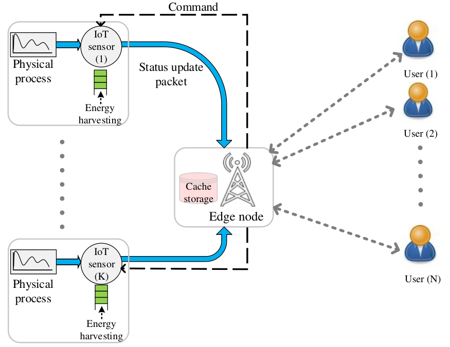
We consider a multi-user multi-sensor IoT sensing network that consists of a set ${\mathcal{K}=\{1,\ldots,K\}}$ of $K$ energy harvesting (EH) sensors, an edge node (a gateway), and a set ${\mathcal{N}=\{1,\ldots,N\}}$ of $N$ users, as depicted in Fig. 1. Users are interested in timely status information about random processes associated with physical quantities $f_{k}$, e.g., speed or temperature, each of which is independently measured by sensor $k\in\mathcal{K}$. We consider request-based status updating, where the users send requests on demand for obtaining status of quantities $f_{k}$, ${k\in\mathcal{K}}$. When a request for the physical quantify $f_{k}$ is generated at the user side, the associated sensor $k$ may send a status update packet that contains the measured value of the monitored process and a time stamp of the generated sample. We assume that there is no direct link between the users and the sensors, i.e., the users receive the status updates only via the edge node.

We consider a time-slotted system with slots indexed by ${t\in\mathbb{N}}$. At the beginning of slot $t$, users send requests for the status of physical quantities $f_{k}$ to the edge node. Let $r_{k,n}(t)\in\{0,1\}$, $t=1,2,\dots$, denote the random process of requesting the status of $f_{k}$ by user $n$; $r_{k,n}(t)=1$ if the status of $f_{k}$ is requested by user $n\in\mathcal{N}$ at slot $t$ and $r_{k,n}(t)=0$ otherwise. The requests are independent across the users, sensors, and time slots. Let $p_{k,n}$ be the probability that the status of $f_{k}$ is requested by user $n$ at each slot, i.e., $\mathrm{Pr}\{r_{k,n}(t)=1\}=p_{k,n}$. Note that there can be multiple users requesting for $f_{k}$ at each slot; $r_{k}(t)=\sum_{n=1}^{N}r_{k,n}(t)\in\{0,1,\ldots,N\}$ indicates the number of requests for $f_{k}$ at slot $t$. We assume that all requests that arrive at the beginning of slot $t$ are handled by the edge node during the same slot $t$. To this end, we assume that all the communication links, i.e., the sensor-edge and edge-user links, are error-free¹¹ 1 The main focus of this paper is to devise effective status updating procedures in a multi-user multi-sensor IoT network under both energy and transmission limitations. Thus, the possibly error-prone communication links are left for future study..

The edge node is equipped with a cache of size $K$ that stores the most recently received status update packet from each sensor. Upon receiving a request for the status of $f_{k}$ at slot $t$, the edge node has two options to serve the request: 1) command sensor $k$ to send a fresh status update, or 2) use the previous measurement from the cache. Let $a_{k}(t)\in\{0,1\}$ be the command action of the edge node at slot $t$; $a_{k}(t)=1$ if the edge node commands sensor $k$ to send an update and $a_{k}(t)=0$ otherwise.

We consider that, due to limited amount of radio resources (e.g., time-frequency resource blocks), no more than $M\leq K$ sensors can transmit status updates to the edge node within each slot. This transmission constraint imposes a limitation to the number of commands as

We refer to $M$ as the transmission budget hereinafter.

We assume that the sensors harvest energy from the environment for sustainable operation. We model the energy arrivals at the sensors as independent Bernoulli processes with intensities $\lambda_{k}$, $k\in\mathcal{K}$. This characterizes the discrete nature of the energy arrivals in a slotted-time system, i.e., at each slot, a sensor either harvests one unit of energy or not (see, e.g., [13, 18, 28]). Let $e_{k}(t)\in\left\{0,1\right\}$, $t=1,2,\dots$, denote the energy arrival process of sensor $k$. Thus, the probability that sensor $k$ harvests one unit of energy during one slot is $\lambda_{k}$²² 2 The scenario where the sensors access to sufficient power (e.g., connected to a fixed power grid) so that they can send a status update at every slot is a special case of our system model, i.e., a unit energy arrival at every slot, $\lambda_{k}=1$., i.e., ${\Pr\{e_{k}(t)=1\}=\lambda_{k}}$, $\forall t$. Sensor $k$ stores the harvested energy into a battery of finite size $B_{k}$ (units of energy). Formally, let $b_{k}(t)$ denote the battery level of sensor $k$ at the beginning of slot $t$, where ${b_{k}(t)\in\{0,\ldots,B_{k}\}}$.

We assume that transmitting a status update from each sensor to the edge node consumes one unit of energy (see, e.g., [4, 13, 18, 21, 28]). Once sensor $k$ is commanded by the edge node (i.e., $a_{k}(t)=1$), sensor $k$ sends a status update if it has at least one unit of energy (i.e., $b_{k}(t)\geq 1$). Formally, let random variable $d_{k}(t)\in\left\{0,1\right\}$ denote the action of sensor $k$ at slot $t$; $d_{k}(t)=1$ if sensor $k$ sends a status update to the edge node and $d_{k}(t)=0$ otherwise. Accordingly, the sensor’s action, the edge node’s action, and the sensor’s battery level are interrelated as

where $\mathds{1}_{\{\cdot\}}$ is the indicator function. Note that $d_{k}(t)$ in (2) characterizes the energy consumption of sensor $k$ at slot $t$. It is also worth noting that by (2), we have $d_{k}(t)\leq{a_{k}(t)}$, and consequently, (1) implies that $\sum_{k=1}^{K}d_{k}(t)\leq M$ for all slots; hence, the name transmission constraint for (1).

Finally, using the defined quantities $b_{k}(t)$, $d_{k}(t)$, and $e_{k}(t)$, the evolution of the battery level of sensor $k$ is expressed as

To measure the freshness of information seen by the users in our request-based status updating system, we use the notion of age of information (AoI) [1] and define on-demand AoI [4]. In contrast to AoI that measures the freshness of information at every slot, on-demand AoI quantifies the freshness of information at the users’ request instants (only).

Let $\Delta_{k}(t)$ be the AoI about the physical quantity $f_{k}$ at the edge node at the beginning of slot $t$, i.e., the number of slots elapsed since the generation of the most recently received status update packet from sensor $k$. Let $u_{k}(t)$ denote the most recent slot in which the edge node received a status update packet from sensor $k$, i.e., $u_{k}(t)=\max\{t^{\prime}|t^{\prime}<t,d_{k}(t^{\prime})=1\}$. Thus, the AoI about $f_{k}$ is given by the random process $\Delta_{k}(t)\triangleq t-u_{k}(t)$.

We make a common assumption (see e.g., [4, 7, 9, 10, 12, 14, 15, 16, 21, 19, 20, 18, 22]) that $\Delta_{k}(t)$ is upper-bounded by a finite value $\Delta^{\mathrm{max}}$, i.e., $\Delta_{k}(t)\in\{1,2,\ldots,\Delta^{\mathrm{max}}\}$. Besides tractability, this accounts for the fact that once the available measurement about $f_{k}$ becomes excessively stale, further counting would be irrelevant. At each slot, the AoI about $f_{k}$ drops to one if the edge node receives a status update from the corresponding sensor, or otherwise, it increases by one. Accordingly, the evolution of $\Delta_{k}(t)$ can be written as

which can be expressed compactly as $\Delta_{k}(t+1)=\min\{(1-d_{k}(t))\Delta_{k}(t)+1,\Delta^{\mathrm{max}}\}$.

We define on-demand AoI for a sensor-user pair $(k,n)$ at slot $t$ as the sampled version of (4) where the sampling is controlled by the request process $r_{k,n}(t)$, i.e.,

In (5), since the requests come at the beginning of slot $t$ and the edge node sends measurements to the users at the end of the same slot, $\Delta_{k}(t+1)$ is the AoI about $f_{k}$ seen by the users.

For the considered system, the energy and transmission constraints pose limitations on when and how often a new status update can be generated at each sensor, which in turn affect the on-demand AoI. Our objective is to keep the on-demand AoI as small as possible, subject to the constraints in the system.

Formally, for a given policy $\pi$, we define the average cost as the average on-demand AoI over all sensors and users, i.e.,

where $\mathbb{E}_{\pi}[\cdot]$ is the (conditional) expectation when the policy $\pi$ is applied to the system and $\mathbf{s}(0)=\big(s_{1}(0),\ldots,s_{K}(0)\big)$ is the initial state³³ 3 It is shown in Proposition 2 that the minimum average cost is independent of the initial state, thus, we omit the initial state henceforth.. We aim to find an optimal policy $\pi^{\star}$ that achieves the minimum average cost, i.e.,

The MDP is defined by the tuple ${\big(\mathcal{S},\mathcal{A},\Pr(\mathbf{s}(t+1)|\mathbf{s}(t),\mathbf{a}(t)),c(\mathbf{s}(t),\mathbf{a}(t))\big)}$, where the state space $\mathcal{S}$ and the action space $\mathcal{A}$ were defined in Section II-D. The cost function $c(\mathbf{s}(t),\mathbf{a}(t))$ represents the cost of taking action $\mathbf{a}(t)$ in state $\mathbf{s}(t)$, which is given by ${c(\mathbf{s}(t),\mathbf{a}(t))={\frac{1}{NK}}\sum_{k=1}^{K}c_{k}(s_{k}(t),a_{k}(t))}$, where the per-sensor cost $c_{k}(s_{k}(t),a_{k}(t))$ is calculated using (6), i.e., $c_{k}(s_{k}(t),a_{k}(t))=r_{k}(t)\min\left\{\left(1-a_{k}(t)\mathds{1}_{\{b_{k}(t)\geq 1\}}\right)\Delta_{k}(t)+1,\Delta^{\mathrm{max}}\right\}$. The state transition probability $\Pr(\mathbf{s}(t+1)|\mathbf{s}(t),\mathbf{a}(t))$ maps a state-action pair at slot $t$ onto a distribution of states at slot $t+1$. The probability of transition from current state $\mathbf{s}(t)=\left(s_{1}(t),\dots,s_{K}(t)\right)$ to next state $\mathbf{s}(t+1)=\left(s_{1}(t+1),\dots,s_{K}(t+1)\right)$ under action $\mathbf{a}(t)=\left(a_{1}(t),\dots,a_{K}(t)\right)$ is factorized as

where $(a)$ follows from the fact that given action $\mathbf{a}$, the state associated with each sensor (i.e., the per-sensor state) evolves independently from the other sensors. Above, the per-sensor state transition probability $\Pr\left(s_{k}(t+1)\mid s_{k}(t),a_{k}(t)\right)$ gives the probability of transition from per-sensor state $s_{k}(t)=\left(r_{k},b_{k},\Delta_{k}\right)$ to next per-sensor state $s_{k}(t+1)=\left(r^{\prime}_{k},b^{\prime}_{k},\Delta^{\prime}_{k}\right)$ under action $a_{k}(t)=a_{k}$, and it is expressed as

where $(a)$ follows from the chain rule, $(b)$ follows from the independence between the request process and the other random variables, $(c)$ follows because, given current battery level $b_{k}$ and action $a_{k}$, next battery level $b_{k}^{\prime}$ is independent of the requests and the current AoI, and $(d)$ follows since given $b_{k}$, $\Delta_{k}$, and $a_{k}$, the next value of AoI $\Delta^{\prime}_{k}$ can be obtained deterministically (see (4)). The probabilities in (10) are calculated in the following.

The random variable $r^{\prime}_{k}=\sum_{n}r^{\prime}_{k,n}$ is a sum of independent Bernoulli trials that are not necessarily identically distributed. Therefore, it has a Poisson binomial distribution [29] as

At each slot, sensor $k$ consumes one unit of energy for sending a status update (i.e., when $a_{k}(t)=1$ and $b_{k}(t)\geq 1$) and harvests one unit of energy with probability $\lambda_{k}$, thus, we have

According to (4) and (2), given current battery level $b_{k}$, AoI $\Delta_{k}$, and action $a_{k}$, the next value of AoI $\Delta^{\prime}_{k}$ can be obtained deterministically. Thus, we have

In this section, we propose an iterative algorithm that obtains an optimal policy $\pi^{\star}$ for (P1). To this end, we first define the accessibility condition for an MDP and prove that our MDP modeling in Section III-A satisfies this condition. Then, we present a proposition that characterizes an optimal policy $\pi^{\star}$ for (P1).

An optimal policy $\pi^{\star}$ can be found by turning the Bellman’s optimality equation (14) into an iterative procedure, called relative value iteration algorithm (RVIA) [31, Section 8.5.5]. Particularly, at each iteration $i=0,1,\ldots$, we have

where ${\mathbf{s}_{\mathrm{ref}}\in\mathcal{S}}$ is an arbitrary reference state. For any initialization $V^{(0)}(\mathbf{s})$, the sequences $\{h^{(i)}(\mathbf{s})\}_{i=1,2,\ldots}$ and $\{V^{(i)}(\mathbf{s})\}_{i=1,2,\ldots}$ converge, i.e., $\lim_{i\to\infty}h^{(i)}(\mathbf{s})=h(\mathbf{s})$ and ${\lim_{i\to\infty}V^{(i)}(\mathbf{s})=V(\mathbf{s})}$, $\forall\mathbf{s}\in\mathcal{S}$. Thus, $h(\mathbf{s})=V(\mathbf{s})-V(\mathbf{s}_{\mathrm{ref}})$ satisfies (14) and $\bar{C}^{\star}=V(\mathbf{s}_{\mathrm{ref}})$. Functions $V$ and $h$ are (sometimes) called value function and relative value function, respectively. It is worth noting that any function $h$ satisfying (14) is unique up to an additive factor, i.e., if $h$ satisfies (14), then $h+\alpha$, where $\alpha$ is any constant, also satisfies (14). The proposed RVIA is presented in Algorithm 1, where $\theta$ is a small constant for the RVIA termination criterion.

It is important to point out that the state space $\mathcal{S}$ and action space $\mathcal{A}$ grow exponentially with respect to the number of sensors $K$, and thus, the complexity of the RVIA presented in Algorithm 1 grows exponentially in $K$. Accordingly, finding an optimal policy $\pi^{\star}$ is practical (tractable) only for small numbers of sensors. To this end, we next propose a low-complexity sub-optimal algorithm whose complexity increases only linearly in $K$.

We relax the constraint (1) and formulate the relaxed problem as a CMDP. To this end, we define the average number of command actions under a policy $\pi_{\mathrm{R}}$ as

and express the relaxed problem as

where $\Gamma\triangleq\frac{M}{K}$ is the normalized transmission budget.

We model (P2) as a CMDP defined by the tuple ${\big(\mathcal{S},\mathcal{A}_{\mathrm{R}},\Pr(\mathbf{s}(t+1)|\mathbf{s}(t),\mathbf{a}(t)),c(\mathbf{s}(t),\mathbf{a}(t))\big)}$, where the state space $\mathcal{S}$ and the relaxed action space $\mathcal{A}_{\mathrm{R}}$ were defined in Section II-D, and $\Pr(\mathbf{s}(t+1)|\mathbf{s}(t),\mathbf{a}(t))$ and $c(\mathbf{s}(t),\mathbf{a}(t))$ were defined in Section III-A. Note that the only difference between the CMDP tuple and the MDP tuple in Section III-A is in the action space ($\mathcal{A}_{\mathrm{R}}$ vs $\mathcal{A}$).

It is worth noting that any policy $\pi$ that satisfies the per-slot transmission constraint (1) satisfies the time average transmission constraint (18) in (P2). Thus, the average cost obtained by following policy $\pi_{\mathrm{R}}^{\star}$ is a lower bound on the average cost obtained under policy $\pi^{\star}$, i.e.,

To solve the CMDP problem (P2), we introduce a Lagrange multiplier $\mu$ and define the Lagrangian associated with problem (P2) as

For a given ${\mu\geq 0}$, we define the Lagrange dual function ${\mathcal{L}^{\star}({\mu})=\min_{\pi_{\mathrm{R}}}{\mathcal{L}}({\pi_{\mathrm{R}},\mu})}$. A policy that achieves ${\mathcal{L}}^{\star}({\mu})$ is called $\mu$-optimal, denoted by $\pi_{\mathrm{R},\mu}^{\star}$, and it is a solution of the following (unconstrained) MDP problem

Since the dimension of the state space $\mathcal{S}$ is finite, the growth condition [32, Eq. 11.21] is satisfied. Moreover, the immediate cost function is bounded below, i.e., $c(\mathbf{s},\mathbf{a})\geq 0$, $\forall\mathbf{a},\mathbf{s}$. Having these conditions satisfied, the optimal value of the CMDP problem (P2), $\bar{C}_{\pi^{\star}_{\mathrm{R}}}$, and the optimal value of the MDP problem (P3), $\mathcal{L}^{\star}({\mu})$, ensures the following relation [32, Corollary 12.2]

Therefore, an optimal policy for (P2) is found by a two-stage iterative algorithm: 1) for a given $\mu$, we find a $\mu$-optimal policy, and 2) we update $\mu$ in a direction that obtains $\bar{C}_{\pi^{\star}_{\mathrm{R}}}$ according to (22). These two steps are detailed in Sections IV-A1 and IV-A2, respectively.

References

- [1] S. Kaul, R. Yates, and M. Gruteser, “Real-time status: How often should one update?” in Proc. IEEE Int. Conf. on Computer. Commun. (INFOCOM), Orlando, FL, USA, Mar. 25–30, 2012, pp. 2731–2735.
- [2] Y. Sun, I. Kadota, R. Talak, E. Modiano, and R. Srikant, “Age of information: A new metric for information freshness,” Synthesis Lectures on Communication Networks, vol. 12, no. 2, pp. 1–224, 2019.
- [3] D. Niyato, D. I. Kim, P. Wang, and L. Song, “A novel caching mechanism for internet of things (IoT) sensing service with energy harvesting,” in Proc. IEEE Int. Conf. Commun., Kuala Lumpur, Malaysia, May 22-27 2016, pp. 1–6.
- [4] M. Hatami, M. Leinonen, and M. Codreanu, “AoI minimization in status update control with energy harvesting sensors,” IEEE Trans. Commun., vol. 69, no. 12, pp. 8335–8351, Dec. 2021.
- [5] Y. P. Hsu, E. Modiano, and L. Duan, “Scheduling algorithms for minimizing age of information in wireless broadcast networks with random arrivals,” IEEE Trans. Mobile Comput., vol. 19, no. 12, pp. 2903–2915, Dec. 2020.
- [6] I. Kadota, A. Sinha, E. Uysal-Biyikoglu, R. Singh, and E. Modiano, “Scheduling policies for minimizing age of information in broadcast wireless networks,” IEEE/ACM Trans. Netw., vol. 26, no. 6, pp. 2637–2650, Dec. 2018.
- [7] A. Maatouk, S. Kriouile, M. Assad, and A. Ephremides, “On the optimality of the Whittle’s index policy for minimizing the age of information,” IEEE Trans. Wireless Commun., vol. 20, no. 2, pp. 1263–1277, Feb. 2021.
- [8] S. Kriouile, M. Assaad, and A. Maatouk, “On the global optimality of Whittle’s index policy for minimizing the age of information,” arXiv preprint arXiv:2102.02528, 2021.
- [9] E. T. Ceran, D. Gündüz, and A. György, “Average age of information with hybrid ARQ under a resource constraint,” IEEE Trans. Wireless Commun., vol. 18, no. 3, pp. 1900–1913, Mar. 2019.
- [10] ——, “A reinforcement learning approach to age of information in multi-user networks with HARQ,” IEEE J. Sel. Areas Commun., vol. 39, no. 5, pp. 1412–1426, May 2021.
- [11] H. Tang, J. Wang, L. Song, and J. Song, “Minimizing age of information with power constraints: Multi-user opportunistic scheduling in multi-state time-varying channels,” IEEE J. Sel. Areas Commun., vol. 38, no. 5, pp. 854–868, May 2020.
- [12] A. Zakeri, M. Moltafet, M. Leinonen, and M. Codreanu, “Minimizing AoI in resource-constrained multi-source relaying systems with stochastic arrivals,” arXiv preprint arXiv:2109.05106, 2021.
- [13] B. T. Bacinoglu, E. T. Ceran, and E. Uysal-Biyikoglu, “Age of information under energy replenishment constraints,” in Proc. Inform. Theory and Appl. Workshop, San Diego, CA, USA, Feb. 1–6 2015, pp. 25–31.
- [14] E. T. Ceran, D. Gündüz, and A. György, “Learning to minimize age of information over an unreliable channel with energy harvesting,” arXiv preprint arXiv:2106.16037, 2021.
- [15] C. Tunc and S. Panwar, “Optimal transmission policies for energy harvesting age of information systems with battery recovery,” in Proc. Annual Asilomar Conf. Signals, Syst., Comp., Pacific Grove, CA, USA, Nov. 3–6, 2019, pp. 2012–2016.
- [16] S. Leng and A. Yener, “Age of information minimization for an energy harvesting cognitive radio,” IEEE Trans. on Cogn. Commun. Netw., vol. 5, no. 2, pp. 427–439, May 2019.
- [17] Z. Chen, N. Pappas, E. Björnson, and E. G. Larsson, “Optimizing information freshness in a multiple access channel with heterogeneous devices,” IEEE Open J. Commun. Soc., vol. 2, pp. 456–470, Mar. 2021.
- [18] G. Stamatakis, N. Pappas, and A. Traganitis, “Control of status updates for energy harvesting devices that monitor processes with alarms,” in IEEE Globecom Workshops (GC Wkshps), Waikoloa, HI, USA, Dec. 9–13, 2019, pp. 1–6.
- [19] E. Gindullina, L. Badia, and D. Gündüz, “Age-of-information with information source diversity in an energy harvesting system,” IEEE Trans. Green Commun. Netw., vol. 5, no. 3, pp. 1529–1540, Sep. 2021.
- [20] M. A. Abd-Elmagid, H. S. Dhillon, and N. Pappas, “AoI-optimal joint sampling and updating for wireless powered communication systems,” IEEE Trans. Veh. Technol., vol. 69, no. 11, pp. 14 110–14 115, Nov. 2020.
- [21] N. Zhao, C. Xu, S. Zhang, Y. Xie, X. Wang, and H. Sun, “Status update for correlated energy harvesting sensors: A deep reinforcement learning approach,” in Proc. Int. Conf. Wireless Commun. and Sign. Proc., Nanjing, China, Oct. 21–23, 2020, pp. 170–175.
- [22] M. Hatami, M. Jahandideh, M. Leinonen, and M. Codreanu, “Age-aware status update control for energy harvesting IoT sensors via reinforcement learning,” in Proc. IEEE Int. Symp. Pers., Indoor, Mobile Radio Commun., London, UK, Aug. 31–Sep. 3 2020.
- [23] M. Hatami, M. Leinonen, and M. Codreanu, “Minimizing average on-demand AoI in an IoT network with energy harvesting sensors,” in Proc. IEEE Works. on Sign. Proc. Adv. in Wirel. Comms., Lucca, Italy, Sep. 27–30, 2021, pp. 1–6.
- [24] B. Yin, S. Zhang, Y. Cheng, L. X. Cai, Z. Jiang, S. Zhou, and Z. Niu, “Only those requested count: Proactive scheduling policies for minimizing effective age-of-information,” in Proc. IEEE Int. Conf. on Computer. Commun. (INFOCOM), Paris, France, Apr. 29–May 2 2019, pp. 109–117.
- [25] F. Li, Y. Sang, Z. Liu, B. Li, H. Wu, and B. Ji, “Waiting but not aging: Optimizing information freshness under the pull model,” IEEE/ACM Trans. Netw., vol. 29, no. 1, pp. 465–478, Feb. 2021.
- [26] J. Holm, A. E. Kalør, F. Chiariotti, B. Soret, S. K. Jensen, T. B. Pedersen, and P. Popovski, “Freshness on demand: Optimizing age of information for the query process,” in Proc. IEEE Int. Conf. Commun., Montreal, QC, Canada, Jun. 14–23, 2021, pp. 1–6.
- [27] F. Chiariotti, J. Holm, A. E. Kalør, B. Soret, S. K. Jensen, T. B. Pedersen, and P. Popovski, “Query age of information: Freshness in pull-based communication,” arXiv preprint arXiv:2105.06845, 2021.
- [28] N. Pappas, Z. Chen, and M. Hatami, “Average AoI of cached status updates for a process monitored by an energy harvesting sensor,” in Proc. Conf. Inform. Sciences Syst. (CISS), Princeton, NJ, USA, Mar. 18–20, 2020, pp. 1–5.
- [29] Y. H. Wang, “On the number of successes in independent trials,” Statist. Sinica, vol. 3, no. 2, pp. 295–312, Jul. 1993.
- [30] D. Bertsekas, Dynamic Programming and Optimal Control, Vol. II, 3rd ed. Athena Scientific, 2007.
- [31] M. L. Puterman, Markov decision processes: discrete stochastic dynamic programming. John Wiley & Sons, 2014.
- [32] E. Altman, Constrained Markov decision processes. CRC Press, 1999, vol. 7.
- [33] F. J. Beutler and K. W. Ross, “Optimal policies for controlled Markov chains with a constraint,” J. Math. Anal. Appl., vol. 112, no. 1, pp. 236–252, Nov. 1985.
- [34] D.-j. Ma, A. M. Makowski, and A. Shwartz, “Estimation and optimal control for constrained Markov chains,” in Proc. IEEE Conf. Decision Contr., Athens, Greece, Dec. 10–12, 1986, pp. 994–999.
- [35] P. Billingsley, Probability and measure, 3rd ed. John Wiley & Sons, 1995.