Solving a directed percolation inverse problemPreprint: APS/123-QED
Abstract
We present a directed percolation inverse problem for diode networks: Given information about which pairs of nodes allow current to percolate from one to the other, can one find a configuration of diodes consistent with the observed currents? We implement a divide-and-concur iterative projection method for solving the problem and demonstrate the supremacy of our method over an exhaustive approach for nontrivial instances of the problem. We find that the problem is most difficult when some but not all of the percolation data are hidden, and that the most difficult networks to reconstruct generally are those for which the currents are most sensitive to the addition or removal of a single diode.
I Introduction
Directed percolation (DP) is a model of spreading processes with a directional bias, such as the flow of fluid downward through a porous medium, the spread of a forest fire under the influence of wind, or the growth of a polymer in a flowing liquid Obukhov 1980. It can also apply to more abstract processes like phase transitions in liquid crystals Takeuchi et al. 2007, interface pinning Tang and Leschhorn 1992, and the proliferation of turbulence in hydrodynamics Pomeau 1986.
If one interprets the flow direction as the time dimension, DP becomes an elegant formulation for the time evolution of the Ising model or a cellular automaton Domany and Kinzel 1984. This interpretation comes with a natural inverse problem: If one observes the state of a cellular automaton at two different times, one can attempt to reconstruct the rules that govern the system’s evolution Springer and Kenyon 2021; Elser 2021. Though this interpretation involves a regular and repeating network such as a square lattice, it is possible to study percolation in random Fan et al. 2012; Lee et al. 2018 or clustered networks Colomer-de Simón and Boguná 2014; Miller 2009 that are more apt to model social networks or the spread of disease. It is also possible to make percolation locally directed without necessarily favoring one particular direction globally, by randomly installing diode-like edges that allow flow one way but not the other Broadbent and Hammersly 1957. One can then calculate properties such as the conductivity or percolation threshold of lattices with such edges Redner 1982; Redner and Mueller 1982; Verbavatz and Barthelemy 2021; De Noronha et al. 2018.
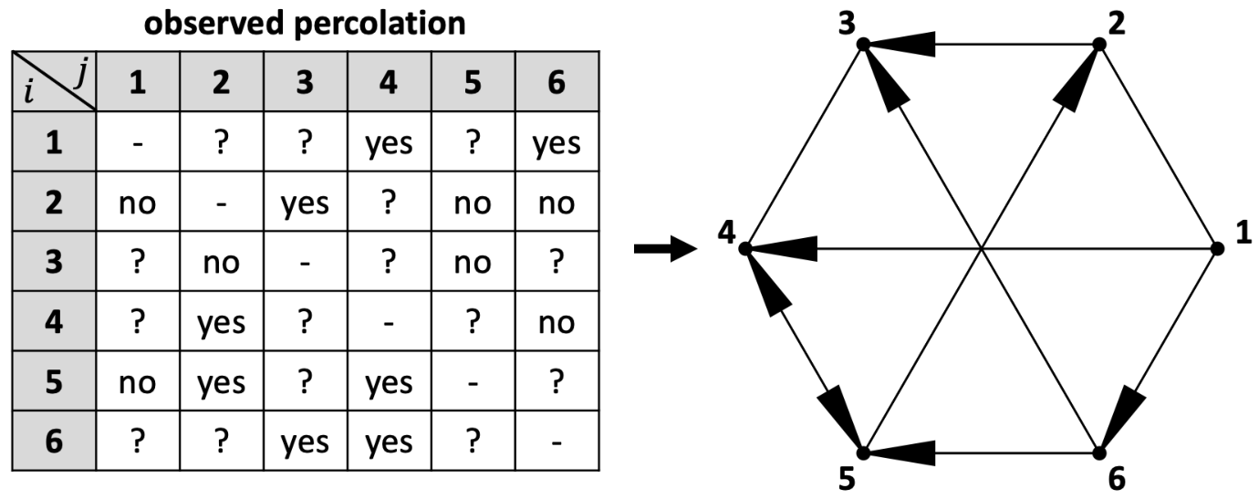
The problem we study in this paper uses diodes as the source of directionality, but not on a lattice. Imagine an electrical circuit consisting solely of nodes, wires, and ideal diodes. Each wire can have
- •
zero diodes, so that current can flow freely in either direction,
- •
one diode, so that current can flow in one direction but not the other, or
- •
two diodes back-to-back, so that current cannot flow in either direction.
Suppose we know which nodes share a wire but we do not know the location or number of diodes. We can apply a voltage across a pair of nodes and record whether current percolates from to . We can do this for several (not necessarily all) pairs of nodes, as in Figure 1. Our task is to find a configuration of diodes consistent with these measurements. Many configurations could yield the same data, so we cannot ask for the configuration that generated the data but merely a configuration consistent with the data. Though we describe it in terms of diodes, this problem can also serve as a model for other systems in which flow is locally asymmetric but occurs in more than one direction globally, such as the spread of information in a social network or the movement of goods or people in a transportation network.
We can pose the problem formally in terms of the adjacency matrix : Let if nodes and share an edge and that edge allows current from to ; otherwise, let . Then gives the number of paths of length from to . Asking if current percolates from to is equivalent to asking whether . Thus, if we know that some elements of are positive, some are zero, and others are completely unknown, our task is to find an consistent with these measurements.
Ours is an inverse problem, like the reconstruction of a cellular automaton, but without the spatial regularity of a lattice or the temporal ordering of time series data. The fact that we are inferring network information from percolation information, rather than the other way around, is perhaps our most salient departure from the canon of percolation problems. This fact makes our problem one of network reconstruction. Such problems are particularly relevant when observational data are available but performing a direct experiment is not possible for logistical or ethical reasons Runge 2018, as in the spread of an infectious disease. We diverge from most other network reconstruction methods in the discreteness and exactness of the solution we seek. Others might search for continuous parameters representing the strength of the interaction between two nodes Sontag 2008 or the concentration of a substance at one node Angulo et al. 2017, or they might seek to winnow down the space of possible networks probabilistically to identify the most likely candidates Peixoto 2019. These methods are appropriate when the network is large, data are relatively plentiful, and probabilistic or continuous descriptions of the network are desirable. We instead seek solutions that definitively specify whether each edge is open and reproduce the observations exactly. These rigid constraints make our method most suitable for reconstructing small networks from scant or incomplete data.
It is possible to convert our problem into a Boolean satisfiability (SAT) problem. Appendix A describes how to do so. The SAT problem was the first to be proven NP-complete Cook 1971, and many other problems—sudoku Lynce and Ouaknine 2006, cryptography Massacci and Marraro 2000, cellular automaton reconstruction Elser 2021, the -queens problem and others Bright et al. 2019—can be posed as SAT problems, making it a useful way to generically evaluate the difficulty of a logical constraint problem. There are several methods Molnár et al. 2018; Ercsey-Ravasz and Toroczkai 2011; Sorensson and Een 2005; Biere 2013; Gravel and Elser 2008 available for solving SAT problems. Mapping our problem into SAT makes it possible in principle to tackle our problem with these methods; however, the number of variables and clauses involved in the corresponding SAT problem scales with the number of self-avoiding paths in the network, which can grow quite quickly with the number of nodes in the network (see appendix A). In a complete network, for example, the number of self-avoiding walks is more than . In the method we present in Section II, the number of variables scales with the number of edges times the number of cells in the data table, a product which is less than .
II Algorithm
The divide-and-concur approach Gravel and Elser 2008 divides a difficult problem with many constraints into a set of easy problems, finds a solution to each easy problem, then tries to make the solutions concur with each other. To apply this approach to our problem, we break the difficult task of finding a configuration of diodes consistent with all observations into a collection of much simpler tasks: For each ordered pair of nodes , find a configuration of diodes consistent with cell of the data table. There are pairs to consider, where is the number of nodes, so this yields configurations. If all of these configurations are the same, then we have solved the problem. If not, we must find a new set of configurations and iterate until they all concur.
Our algorithm formulates this task as a search for a point in the intersection of two sets in a high-dimensional Euclidean space. Let be the set of directed edges in the network. For each pair we create a set of variables . A setting of means there is a diode blocking directed edge in the configuration generated for pair , and means there is no such diode, but during the search process we will allow to be any real number. We use the shorthand to denote the vector containing all of the ’s.
Let be the set of such that all are or , and for each the diode configuration encoded by is consistent with cell of the data table. The projection of to set is the point such that the distance
| (1) |
is as small as possible. Projecting an arbitrary to the nearest point in can be computationally expensive, so we use a quasi-projection: It always gives a point in set , but not necessarily the distance-minimizing point.
The quasi-projection is implemented as follows. We know we must set all to either or . So our first step is to set
| (2) |
for all and . If all we had to do was set the variables to or , then we would be done here and this would be an exact projection. However, ensuring that each agrees with the data will involve changing some ’s to ’s and vice versa. The squared distance for setting is
and for it is
so is the “extra distance” for changing from to , and is the extra distance for changing a to a .
Now, to ensure agrees with the data for :
- •
If there are no data for , do nothing.
- •
If the data indicate current percolates from to , check if there is at least one path from to with along every directed edge of the path. If there is no such path, rank the paths by the extra distance for opening the path: For a given edge , if then we have and we incur an extra distance of to change to . If then we already have and there is no extra distance. Thus, we can write the total extra distance for the path as
For the path with the lowest sum, set for every on the path.
- •
If the data indicate current does not percolate from to , then for every path from to , check if at least one edge along the path has . For any path for which this is not so, choose the on that path with the largest (i.e., smallest ) and set .
This last point, the method for blocking current, is what makes our projection a quasi-projection, as it is not strictly distance-minimizing. See Appendix B for an illustrative example.
Projecting to solves all of the easy problems; what remains is to make these solutions concur. For this we define as the set of such that for each , all are equal. (This does not require that or .) Projecting to is a simple average:
| (3) |
Any is a solution to our problem.
We initialize with random real numbers between and , then iterate using a generalized Douglas-Rachford method Aragón Artacho et al. 2020:
| (4) |
where is the reflection of across , and likewise for . Using reflections, rather than just projections, is critical to allow the algorithm to escape from non-solution traps where and come close but do not intersect Aragón Artacho et al. 2020. One can check that if is a fixed point of (4), then . The parameter controls the size of the iteration steps. Taking gives a reliable, continuous trajectory but makes the search process slow. Larger () can make the search quicker but sometimes leads the algorithm to get stuck in limit cycles. In this paper we use a conservative value, , so that the algorithm avoids this limit-cycle trapping in all but a few percent of trials.
Finally, we note that there are other realizations of the divide-and-concur principle for this problem. Having briefly tested some alternatives, we can say that the choice of implementation can affect the algorithm’s performance but for the most part does not affect the major patterns we will describe in Section III.
- •
One speed-up is to have only for the pairs for which the percolation data are known. If some of the data are hidden, this mean fewer pairs to handle in the projection, which makes each iteration faster. However, we find that it can also make the algorithm more likely to get trapped in limit cycles, particularly when only two or three pairs in the data table are known.
- •
One can also take advantage of the percolation data for ordered pairs that happen to share an edge: For every directed edge , if we observe no percolation from to , we can permanently set for all . If we do observe percolation from to , we can safely set for all . By not using these shortcuts in our implementation we are effectively asking the algorithm to be clever enough to discover them on its own.
- •
If speed is no concern but the exactness of the projection is, one can create variables for every path , not just every pair. This makes our approach of blocking path by path an exact projection, but the enormous number of variables makes the algorithm much slower.
This is not an exhaustive list of alternative implementations, but it illustrates the diversity of approaches to solving a problem in the divide-and-concur framework. The framework is also quite adaptable to extra global constraints. For example, if one wanted to impose a maximum or minimum number of diodes, one could add an extra step in the projection that computes and, if the sum does not satisfy the max/min requirement, add a constant to all of the to ensure it does. Implementing such a constraint would be less straightforward if one chose to solve this problem with, say, the SAT formulation in Appendix A.
III Experiments
In the experiments that follow, we avoid trivial instances of the problem as much as possible. One obvious trivial instance is when all of the current data are hidden, in which case there are no constraints and thus any configuration of any number of diodes is a solution. However, when none of the data are hidden there are more than enough constraints—enough for one to construct a solution by hand: For any that share a wire and for which current does not flow from , place a diode on wire to prevent current from . These diodes alone are sufficient to solve the problem. (See Appendix C for a proof.) So to keep things nontrivial we hide exactly half of the data, except in section III.2 when we explore how the difficulty of the problem depends on the number of hidden data.
The problem is also trivial if there are no wires, in which case there is no current and nowhere to put any diodes. But in a network with a wire between every pair of nodes, once again there is a by-hand construction: Place diodes blocking every directed edge except those for which we know current can flow from to . Even if the data are incomplete, these diodes solve the problem. (See Appendix C for a proof.) So apart from section III.4, in which we vary the number of wires, we use a type of bipartite network that has roughly half of its possible wires: We take an even number of nodes and let nodes and share a wire if is odd.

The example in Figure 1 is a typical nontrivial instance—a bipartite network with half of the data hidden. Figure 2 illustrates the behavior of our algorithm as it tries to solve such an instance. The upper panel shows the evolution of the concur estimate , with each row corresponding to for a single directed edge . (Since is the same for all , we can drop the from the subscript.) White corresponds to closer to , meaning that the algorithm thinks there should be a diode on edge , while black indicates no diode. Gray shades indicate the algorithm is uncertain, or is “changing its mind” and adding or removing that diode. The lower panel plots the error, which we define as the RMS of
Comparing the upper and lower panels of Figure 2, one can see that the spikes in the error time series coincide with moments when the algorithm adds or removes a diode. Suddenly, after about iterations the error drops by many orders of magnitude, reflecting the “aha moment” when the algorithm has found a solution. In practice, we let the algorithm stop and declare success once the error falls below .
III.1 Scaling with
| projection | exhaustive | |
|---|---|---|
The most obvious parameter of our problem is the number of nodes, and it is important to know how our method scales with . For each even from to we randomly generated networks, with the number of diodes chosen to maximize the difficulty of the problem for our algorithm (see Section III.3), then hid half of the current data. To provide a comparison for our algorithm, we also implemented an exhaustive “brute force” solution finder, which simply lists all of the possible solutions and checks them one by one until finding one that works.
Table 1 gives the average time required for our projection method and the exhaustive approach. The computational expense grows quite quickly for the projection algorithm: From to the time required increases by five orders of magnitude. However, the exhaustive approach scales much worse: The required time grows by eight orders of magnitude just from to . We have not attempted using the exhaustive checker for .
One can understand the growth of the search time by considering what each method actually does. In principle, each iteration of our algorithm may involve checking every possible path for current from any one node to any other. We only consider self-avoiding paths, because any path that visits a node more than once is irrelevant as far as current is concerned, but the number of such paths can still grow with . Meanwhile, the exhaustive approach has to contend with undetermined diodes, yielding possible solutions. Factorial growth may be fast, but grows faster. For large networks the exhaustive approach is simply infeasible.
III.2 Hiding data
In Appendix C we prove that the problem is trivial when all or none of the data are hidden. We will now explore how the algorithm behaves in the two trivial extremes and all the cases in between.
For a given the number of hidden data can be any integer from to . For each we generated instances, once again with the number of diodes for each chosen to maximize the difficulty, and recorded the average number of iterations required to find a solution.
Figure 3 plots the results. Beginning from the required number of iterations increases as more data are hidden. The logarithmic scale disguises the magnitude of this effect somewhat: The number of iterations when half of the data are hidden is actually about twice as many as when none of the data are hidden. However, as continues increasing there comes a point at which the algorithm begins to find solutions much more quickly, particularly when reaches .
Every entry in the data table is a constraint that limits the space of possible solutions. When very few of the data are hidden the algorithm seems to take advantage of the many constraints, finding solutions in fewer and fewer steps as approaches . A human does much the same thing in constructing a solution by hand for (see Appendix C). On the other hand, when most of the data are hidden, the problem is underconstrained and there are many possible solutions. It is natural that the algorithm finds solutions quite easily in this regime—especially when , as that is the case in which any network is a solution.
III.3 Number of diodes
Next we explore how the number of diodes affects the difficulty of the problem. The number of diodes can be any integer from to the number of directed edges , which is for our bipartite networks. For each we have the algorithm attempt to solve networks with randomly placed diodes. In each instance we hide exactly half of the data and record the average number of iterations required to reach a solution.
Figure 4 plots the results. For each the required number of iterations is generally small when is near or , with a peak somewhere in between. The peak shifts farther to the right as increases.
In order to understand this behavior, consider the influence of the diodes on the current percolations of a network. The top panel of Figure 5 shows the current probability—the likelihood that current can percolate from one randomly chosen node to another—as a function of . There is a range of small for which current almost always flows, and this range extends farther to the right as increases. As , the current probability for any approaches linearly.
Both limits make sense intuitively: Current is very likely to flow when the number of diodes is small. Having more nodes allows many more paths, so as increases it takes many more diodes to block all the paths from one node to another. On the other hand, when is almost maximal the number of node-pairs for which current percolates is simply the number of directed edges that have not been blocked by a diode, , which does indeed approach linearly as .
The middle panel of Figure 5 gives what we call the current sensitivity, which is simply the magnitude of the slope of the upper panel. The slope is essentially the typical number of percolations that are affected by adding or removing a single diode, so a steeper slope corresponds to a more sensitive network. The current sensitivity curves are qualitatively similar to the curves in Figure 4: small on either side, with a peak that shifts to the right as increases.
To make the similarity more obvious, in the lower panel of Figure 5 we re-plot the data from Figure 4 with a few modifications: First, we plot with a linear rather than logarithmic vertical axis. Second, we subtract off the number of iterations it takes for a completely trivial instance with all of the data hidden. We are essentially removing the part of the search at the far right of Figure 2, when the algorithm has found an answer and is simply converging to reach our desired stopping error (). This turns out to be about iterations, regardless of . Finally, since the larger networks take significantly more iterations, we divide the number of iterations by the square of the number of possible diodes, . Our original motivation for doing so is simply that it makes all of the curves roughly the same magnitude and therefore easy to plot on a linear scale, but in fact it turns out to be a very good rescaling—the plots of this modified iteration number are remarkably similar to the plots of current sensitivity, not only in shape but also in magnitude.
We are hesitant to make any strong claims about whether the similarity of the magnitudes is meaningful, but we are confident that the similar shapes are no coincidence. The networks that require more iterations to solve tend to be those with greater current sensitivity. In other words, the hardest networks to solve are those for which the current percolations are most affected by adding or removing a single diode. Since the algorithm’s task is to match the percolation data by adding and removing diodes, it makes sense that the task is more difficult when the currents are more sensitive.
III.4 Number of wires
Finally, we depart from our bipartite networks and explore how the number and placement of wires affects the difficulty of the problem. For a network with nodes the number of wires can be any integer from to . Here we will give results for networks of size . The behavior for other values of is similar. For each , the number of diodes can be any integer from to . For each we generated networks, hid half of the data, and recorded the number of iterations needed to find a solution.
There are many ways in which one can remove wires. One option is to prune at random. Another approach is to disconnect the network as quickly as possible: Pick a node and remove all the wires that connect to it before touching any other wires. Let us call this the recursive method, because once the chosen node is disconnected one can repeat the process with the remaining nodes. Alternatively, one might delay disconnection as long as possible. One way to do this is to pick two nodes and remove the wire they share. Then pick a third node and remove the wires it shares with the first two. Then pick a fourth node and remove the wires it shares with the first three, and so on. We call this the star method, because once we have picked all but one of the nodes we are left with a star graph (in which the unpicked node is the center and the remaining wires connect the center to the other nodes). Removing the last wires from the star completes the pruning.
How much does the pruning order matter? To find out, in Figure 6 we plot the average iteration count as a function of for each of the three methods. As in sections III.1 and III.2, we are choosing to maximize difficulty: For each we select the that requires the most iterations to solve. The difficulty almost always grows monotonically with , with little difference between the methods. The disparity between the recursive and star methods is greatest at , the moment at which the star method has produced a star graph. An astute observe may notice that the iteration count for the recursive method is higher at than . This coincides with the moment the network of nodes becomes disconnected, leaving a single isolated node and the other nodes completely connected by wires. The same phenomenon occurs between and , the moment when the next node becomes isolated and the remaining are completely connected.
If all one cares about is the most difficult diode configuration for a given , then the order in which one removes wires does not seem to matter much. But what about the pattern from section III.3 in which the iteration count was proportional to the current sensitivity: Is this true for all ?
Figure 7 plots the current probability, current sensitivity, and average number of iterations (rescaled in the same way as in section III.3) for the recursive pruning method, with lighter color corresponding to fewer wires. Thanks to recursion we only need to plot the results from down to . After that it reduces to the analogous problem for . These results echo those of section III.3 in that the rescaled iteration count is roughly proportional to the current sensitivity, with the possible exception of the lightest curve, corresponding to .
Figure 8 plots the current probability, current sensitivity, and average number of iterations for the star pruning method. This time we must take from all the way down to before the network becomes disconnected. Here we see a significant discrepancy between the iteration count and the current sensitivity, particularly for the networks with the fewest wires and relatively few diodes.
Evidently the pattern from section III.3 is not universal. It holds for well-connected networks with many paths from one node to another, such as the bipartite networks used in most of this paper, but it falters for more sparse networks, especially those with “peninsular” nodes that only have one wire connecting them to the rest of the network. Indeed, the curve in Figure 7, the first in which we noticed a discrepancy between iteration count and current sensitivity, corresponds to the network with one node connected to the rest of the network by just a single wire. For the star method, the peninsulas appear at —precisely the networks for which the discrepancy becomes most obvious in Figure 8.
IV Conclusion
We have demonstrated a divide-and-concur iterative projection method for solving a percolation inverse problem in diode networks. Though the computational expense of our method grows rapidly with the size of the network, it grows much slower than that of the exhaustive approach, making our method far more practical for networks with more than a few nodes.
We find that the projection algorithm generally requires more iterations to find a solution when one hides some of the current data, but only up to a point: If nearly all of the data are hidden the lack of constraints makes the problem very easy to solve. We have also used our algorithm to explore how the difficulty of the problem depends on the number of diodes in the network. Our results suggest that the most difficult networks are those for which the currents are most sensitive to the addition or removal of a single diode, although this pattern breaks down for highly pruned networks in which many nodes only have a single wire.
V Acknowledgments
The author thanks Veit Elser (who helped to conceive of this problem), Paul McEuen, and James Sethna for valuable feedback and conversations.
Appendix A Mapping to SAT
The SAT problem is typically formulated in conjunctive normal form (CNF): One is given a list of disjunctive clauses, such as , where each is a Boolean variable. Each can appear in several different clauses, and the task is to find values for the that make every clause true—that is, to satisfy the conjunction of all the clauses.
It is possible to convert our task into a SAT problem. Let be the set of (self-avoiding) paths from to . Observing no current from to means every path is blocked, a fact which is easily expressed in CNF:
| (5) |
If current is observed, it means at least one path is unblocked, which is most naturally written as a disjunction of conjunctions:
| (6) |
There is more than one way to convert a disjunction of conjunctions to a conjunction of disjunctions. The most direct method converts conjunctions of length to disjunctions. For example,
| (7) |
However, this is likely to produce an unacceptable number of clauses. For our bipartite networks with , there are self-voiding paths of length from one node to another (if one node is odd and the other is even) or paths of length (if both nodes are odd or both even). This would yield either or clauses, just for one current observation (without even considering paths of other lengths). A more practical method is to introduce extra Boolean variables: Let there be a for every . Then
| (8) |
has the same satisfiability as (6). Unfortunately, this still requires the introduction of a new variable for each path involved.
It is worth noting that the CNF approach handles the no-current constraints quite naturally but is rather less elegant for the pairs that do have current, whereas our algorithm (Section II) has a straightforward projection for the pairs with current but uses a quasi-projection to handle the no-current pairs. Perhaps a combined approach—using our method for the current pairs and CNF for the no-current pairs—could work more efficiently than either method alone.
Appendix B The quasi-projection to set
Our quasi-projection to always finds a point in set , but there are some circumstances in which it does not select the closest point in .
Suppose that no current was observed for pair and that, after the initial rounding of all to or as prescribed in Eq. (2), two paths need to be blocked. That is, both paths had on all of their edges . The extra distance for changing from to is
For each path individually, the best move is to block the edge with the largest . Let be that edge for path , and likewise for path . For definiteness, suppose , so that the added distance for blocking each path is . But if the two paths share an edge with , then blocking is actually the best move overall, adding a distance of only compared to .
Admittedly, this is a contrived example, and in practice such situations do not seem to prevent the algorithm from finding solutions.
Appendix C Constructing a solution by hand
Suppose we know whether current can percolate from to for every . For any that share a wire and for which current does not flow from , we must place a diode on wire that will prevent current from . We have to place these diodes because otherwise current would flow from , in violation of our data.
Claim C.1.
This placement of diodes solves the problem.
Proof.
Suppose current can percolate from to in the actual circuit used to generate the data; that is, there exists a percolation path from to . We can break the path into steps: , …, . Then current also percolates from to , so we must have left unblocked in our solution circuit. The same holds for every other step in the path. Concatenating these steps together shows that current can percolate from to in our solution circuit.
In the converse direction, suppose current has a path from to in our solution circuit. Again, we can break the path into steps: , …, . We would have blocked in our solution circuit if the data had told us current does not flow from to , so the fact that we did not implies that current can percolate from to in the actual circuit. The same holds for every other step in the path. Any complete dataset generated from an actual circuit has current transitivity: If we observe current from and then we must also observe current from . Thus, by the transitive property we conclude that current can percolate from to in the actual circuit. ∎
The reasoning in the converse direction breaks down if we do not have complete data. There may be percolations in our solution that are forbidden in the actual circuit.
However, if the network is completely connected then there is another construction that will work even with incomplete data: Place diodes blocking every directed edge except those for which we know current can flow from to .
Claim C.2.
This placement of diodes solves the problem: The solution may not have the same percolations as the circuit that generated the data, but it is consistent with all the available data.
Proof.
Suppose the data indicate that current can percolate from to . Then we did not place a diode blocking in our solution circuit, so there is certainly a path from to in our solution circuit. The contrapositive of this implication is that if there is no percolation from to in our circuit, then there is no percolation from to in the data table: The data table either says no percolation, or it contains no information on . Either way, we are consistent with the data.
Now suppose there is a percolation path from to in our solution circuit, and break the path into steps: , …, . We would not have left unblocked in our solution circuit unless the data told us current flows from to , so the data must indicate that current percolates from to . The same holds for every other step in the path. By the transitive property discussed above, current can percolate from to in the circuit that generated the data. So the data table either says so, or it contains no information on . Once again, we are consistent with the data. ∎
The hypothesis of complete connectivity is necessary: If the network is not completely connected, there may be a pair of nodes that do not share a wire, but do have percolation according to the data. The direct path does not exist in this case, so we cannot guarantee that our solution allows percolation from to .
There are surely other ways to construct solutions, but we consider these the simplest. In restricting ourselves to cases in which these constructions fail, we are in essence asking our algorithm to be more clever than we have been in making these constructions. At some point it becomes more time-consuming to come up with better constructions than to simply implement our algorithm.
References
- Obukhov (1980) S. Obukhov, Physica A: Statistical Mechanics and its Applications 101, 145 (1980).
- Takeuchi et al. (2007) K. A. Takeuchi, M. Kuroda, H. Chaté, and M. Sano, Physical review letters 99, 234503 (2007).
- Tang and Leschhorn (1992) L.-H. Tang and H. Leschhorn, Physical Review A 45, R8309 (1992).
- Pomeau (1986) Y. Pomeau, Physica D: Nonlinear Phenomena 23, 3 (1986).
- Domany and Kinzel (1984) E. Domany and W. Kinzel, Physical review letters 53, 311 (1984).
- Springer and Kenyon (2021) J. M. Springer and G. T. Kenyon, in 2021 International Joint Conference on Neural Networks (IJCNN) (IEEE, 2021) pp. 1–8.
- Elser (2021) V. Elser, Phys. Rev. E 104, 034301 (2021).
- Fan et al. (2012) J. Fan, M. Liu, L. Li, and X. Chen, Physical Review E 85, 061110 (2012).
- Lee et al. (2018) D. Lee, B. Kahng, Y. Cho, K.-I. Goh, and D.-S. Lee, Journal of the Korean Physical Society 73, 152 (2018).
- Colomer-de Simón and Boguná (2014) P. Colomer-de Simón and M. Boguná, Physical Review X 4, 041020 (2014).
- Miller (2009) J. C. Miller, Physical Review E 80, 020901 (2009).
- Broadbent and Hammersly (1957) S. R. Broadbent and J. M. Hammersly, Math. Proc. Cambridge Philosophical Soc. 53, 629 (1957).
- Redner (1982) S. Redner, Phys. Rev. B 25, 3242 (1982).
- Redner and Mueller (1982) S. Redner and P. R. Mueller, Phys. Rev. B 26, 5293 (1982).
- Verbavatz and Barthelemy (2021) V. Verbavatz and M. Barthelemy, Physical Review E 103, 042313 (2021).
- De Noronha et al. (2018) A. W. De Noronha, A. A. Moreira, A. P. Vieira, H. J. Herrmann, J. S. Andrade Jr, and H. A. Carmona, Physical Review E 98, 062116 (2018).
- Runge (2018) J. Runge, Chaos: An Interdisciplinary Journal of Nonlinear Science 28, 075310 (2018).
- Sontag (2008) E. Sontag, Essays in Biochemistry 45, 161 (2008).
- Angulo et al. (2017) M. T. Angulo, J. A. Moreno, G. Lippner, A.-L. Barabási, and Y.-Y. Liu, Journal of the Royal Society Interface 14, 20160966 (2017).
- Peixoto (2019) T. P. Peixoto, Physical review letters 123, 128301 (2019).
- Cook (1971) S. A. Cook, in Proceedings of the third annual ACM symposium on Theory of computing (1971) pp. 151–158.
- Lynce and Ouaknine (2006) I. Lynce and J. Ouaknine, ISAIM 11, 6 (2006).
- Massacci and Marraro (2000) F. Massacci and L. Marraro, Journal of Automated Reasoning 24, 165 (2000).
- Bright et al. (2019) C. Bright, J. Gerhard, I. Kotsireas, and V. Ganesh, in Maple Conference (Springer, 2019) pp. 205–219.
- Molnár et al. (2018) B. Molnár, M. Varga, Z. Toroczkai, and M. Ercsey-Ravasz, A high-performance analog max-sat solver and its application to ramsey numbers (2018).
- Ercsey-Ravasz and Toroczkai (2011) M. Ercsey-Ravasz and Z. Toroczkai, Nature Physics 7, 966 (2011).
- Sorensson and Een (2005) N. Sorensson and N. Een, SAT 2005, 1 (2005).
- Biere (2013) A. Biere, Proceedings of SAT competition 2013, 1 (2013).
- Gravel and Elser (2008) S. Gravel and V. Elser, Physical Review E 78, 036706 (2008).
- Aragón Artacho et al. (2020) F. J. Aragón Artacho, R. Campoy, and M. K. Tam, Mathematical Methods of Operations Research 91, 201 (2020).