跳到论文正文
W Papers独立论文阅读器 arXiv:2201.12052 论文正文 计算阅读时间 · 0%
引用这篇论文根据当前论文元数据生成,正式投稿前建议核对。


License: CC BY 4.0
arXiv:2201.12052v2 [cs.LG] 16 Nov 2022

Improved Overparametrization Bounds for Global Convergence of SGD for Shallow Neural Networks

Bartłomiej Polaczyk Address: Institute of Informatics, University of Warsaw, Banacha 2, Warsaw, Poland. and Jacek Cyranka Email address: b.polaczyk@mimuw.edu.pl (BP) Email address: j.cyranka@mimuw.edu.pl (JC)
Abstract.

We study the overparametrization bounds required for the global convergence of stochastic gradient descent algorithm for a class of one hidden layer feed-forward neural networks equipped with ReLU activation function. We improve the existing state-of-the-art results in terms of the required hidden layer width. We introduce a new proof technique combining nonlinear analysis with properties of random initializations of the network.

1. Introduction

The study of convergence properties of mini-batch stochastic gradient descent (SGD) iterations applied to feed-forward neural nets (NN) is at the core of modern machine learning research. SGD with its variants like ADAM is the most common optimization scheme applied for supervised training of NN. In principle however, the loss landscape encountered when training NN is highly nonconvex, especially for deep nonlinear NN as revealed, e.g., by visualizations performed by Li et al. 2018, and construction proofs of spurious local minima by Auer et al. 1996a; Brutzkus et al. 2018. The nonconvexity may have severe consequences for practical NN training routines, as SGD may potentially get stuck at a spurious local minimum or a saddle point and cease to converge further down the loss valley. Yet, practice suggests that with enough overparametrization, SGD iterations achieve global minima most of the times. This phenomenon is not fully understood yet and is the main theme of this paper.

Contemporary research on NN convergence theory was initiated with the study of linear networks. The loss landscape in this setting was fully characterized by Kawaguchi 2016, solving the problem stated by Choromanska et al. 2015. The research revealed the feasibility of global SGD convergence for deep NN despite the loss landscape nonconvexity.

Even though it seems difficult to fully characterize the loss landscape in the nonlinear setting, proving the global SGD convergence is still feasible. Recent research suggests that SGD converges globally with high probability for random initialization of weights, under the assumption of sufficiently large overparametrization expressed in terms of NN layers’ widths. The first result of this kind required an unrealistic level of overparametrization of polynomial order in the number of samples, cf. Allen-Zhu et al. 2019. The following series of related results (see Table 1) further reduced the required level of overparametrization using various techniques and assumptions on training data. Especially in the case of Deep NN equipped with analytic activation functions, an overparametrization of the linear order with respect to the number of training examples is sufficient. However, such tight overparametrization results do not apply in the case of a non-differentiable ReLU activation function (see Table 1). Existing theoretical bounds still require a significantly larger number of parameters than used in practice. The question about an exact boundary marking the minimal number of parameters required for the global convergence is still open even for shallow (one hidden layer) ReLU NN, see, e.g., Oymak and Soltanolkotabi 2020.

1.1. Main Contribution.

We establish a new theoretical order of overparametrization required for SGD convergence towards a global minimizer for one hidden layer NN with ReLU activations, improving known state-of-the-art bounds. We introduce a new proof technique based on nonlinear analysis. First, we show the global convergence of continuous solutions of the differential inclusion (DI) being a nonsmooth analog of the gradient flow for the MSE loss. Second, using the existing nonsmooth analysis results, we establish closeness of continuous trajectories to SGD sequences until convergence for a sufficiently small learning rate.

The concept of studying the dynamics of continuous solutions pursued in this work already appeared earlier Arora et al. 2019a; Du et al. 2019b. However, the authors treated the convergence of SGD sequences independently from the analysis of continuous solutions, which served motivational purpose only. We develop a rigorous method for for establishing the convergence of SGD sequences via the convergence of continuous solutions, which works for general nonsmooth approximators including deep NN and general loss functions.

1.2. Informal statements.

We derive the global convergence results under the following assumptions and notation (made precise later on). Let NN be the sample size. The input data comes from the i.i.d. sub-Gaussian distribution on the sphere in ℝd0\mathbb{R}^{d_{0}}, where d0∈[Nδ0,N]d_{0}\in[N^{\delta_{0}},N] for some δ0∈(0,1)\delta_{0}\in(0,1). The initial weight vector θ0\theta_{0} is obtained via LeCun scheme (variance scales with width). ℒ⁡(θ)\mathcal{L}(\theta) is the MSE loss for some output matrix, weight vector θ\theta and NN equipped with ReLU activation function. The subdifferential in the sense of Clarke is denoted by ∂\partial and Ω~\tilde{\Omega} is the Ω\Omega notation hiding the logarithmic terms. All presented results hold with high probability (WHP), meaning that the probability of the event converges to one as the number of samples NN diverges to infinity, a convention widely adopted in the literature.

Our first main result provides a condition for the global convergence of the continuous solutions of the nonsmooth analog of gradient flow for ℒ\mathcal{L}.

Theorem 1.1 (Informal Corollary 4.5).

Let the width of the shallow NN satisfy d1=Ω~​(N1.25).d_{1}=\tilde{\Omega}(N^{1.25}). Then, any solution θ:ℝ+→ℝ\theta\colon\mathbb{R}_{+}\to\mathbb{R} to the DI Cauchy problem θ⁡(0)=θ0\theta(0)=\theta_{0}, θ˙(t)∈−∂ℒ(θ(t))\dot{\theta}(t)\in-\partial\mathcal{L}(\theta(t)) satisfies ℒ⁡(θ⁡(t))≤ℒ⁡(θ⁡(0))​exp⁡(−c​t​d1)\mathcal{L}(\theta(t))\leq\mathcal{L}(\theta(0))\exp(-ctd_{1}) for all t≥0t\geq 0 and some constant c>0c>0 WHP.

The second main result establishes the global convergence for the mini-batch SGD iterates WHP.

Theorem 1.2 (Informal Theorem 5.1).

Let the width of the shallow NN satisfy d1=Ω~​(N1.25)d_{1}=\tilde{\Omega}(N^{1.25}). Then, for any error ε>0\varepsilon>0 and any mini-batch size, the mini-batch SGD sequences with step size small enough achieve the loss value below ε\varepsilon at a linear convergence rate WHP.

We obtain Theorem 1.2 via the following result. It is stated for general approximators (including deep ReLU NN) and general losses (including hinge loss, cross-entropy etc.). We believe it is of independent interest. We drop the assumption on the MSE loss and particular NN, and use the notion of an arbitrary loss ℒ~\tilde{\mathcal{L}}.

Theorem 1.3.

(Informal Theorem 5.6) Let the loss function ℒ~\tilde{\mathcal{L}} be arbitrary satisfying some mild technical conditions. Additionally, assume there exists a nonempty compact set QQ, s.t. any solution θ\theta to the DI θ˙(t)∈−∂ℒ~(θ(t))\dot{\theta}(t)\in-\partial\tilde{\mathcal{L}}(\theta(t)) if initialized in QQ, remains in some compact set GG and converges to zero as ℒ~​(θ⁡(t))≤ℒ~​(θ⁡(0))​e−γ​t\tilde{\mathcal{L}}(\theta(t))\leq\tilde{\mathcal{L}}(\theta(0))e^{-\gamma t}. Then, for any ε>0\varepsilon>0, the SGD sequences initialized in QQ and with step size small enough achieve the loss value below ε\varepsilon at a linear convergence rate WHP.

Let us comment briefly on some key aspects of our results.

Overparametrization Bound Improvement.

Theorem 1.2 improves state-of-the-art overparameterization bounds for global SGD convergence for shallow ReLU NN – in Table 1 we compare it to the selected works that we find most related. For instance, Nguyen 2021 require d1=Ω⁡(N2)d_{1}=\Omega(N^{2}). Similarly, Oymak and Soltanolkotabi 2020 require d1=Ω⁡(N4/d03)d_{1}=\Omega(N^{4}/d_{0}^{3}) (which is better for d0d_{0} in a small neighborhood of NN), where they train the first weight matrix only and the second weights matrix remains fixed, cf. Remarks 5.3 and 5.4 for a detailed discussion and Section 6 for numerical experiments comparing both setups. We also note that we have more general data assumptions than Oymak and Soltanolkotabi 2020.

On the other hand, results from Kawaguchi and Huang 2019 and Liu et al. 2022 require only linear overparametrization and work for more general data. However, they do not apply to ReLU as they rely heavily on the smoothness of the activation function. In particular, analysis of non-smooth activation functions seems to be a much more challenging task, see e.g., a result showing the existence of spurious local minima in the ReLU setting Safran and Shamir 2018.

Discrete vs Continuous Convergence.

The idea of establishing a link between continuous solutions to the gradient flow and their discrete GD analogs for deep linear networks was introduced recently by Elkabetz and Cohen 2021. Their method require the Hessian to exist and to be bounded along the continuous trajectories. Such approach does not work when a nonsmooth activation function, e.g. ReLU, is employed – we provide additional evidence supporting this claim in Section 6. Our approach of passing from continuous solutions to SGD sequences is more general because it works in the differential inclusions setting, which treats nondifferentiable objectives (in contrast to Elkabetz and Cohen 2021).

SGD step size.

One should keep in mind that Theorem 1.2 is qualitative – it does not provide a constructive condition for the step size to guarantee convergence. However, existing quantitative results for ReLU NNs give to the best of our knowledge no better bound than 𝒪⁡(1/N2)\mathcal{O}(1/N^{2}), which is still far from the learning rates used in ML practice.

Table 1. A Perspective on related work. Reported results using notation Ω~\widetilde{\Omega} hides logarithmic terms, NN is the number of train samples, d0d_{0} is the input dimension, LL is the number of layers of deep NN
Work Algorithm ReLU Deep Data Scaling
Du et al. 2019a GD no yes non degeneratenormalized\begin{array}[]{c}\text{non degenerate}\\ \text{normalized}\end{array} Ω~​(2O⁡(L)​N4)\tilde{\Omega}(2^{O(L)}N^{4})
Kawaguchi and Huang 2019
GD no yes normalized Ω~​(N​d0)​(shallow)Ω~​(N+d0​L2)​(deep)\begin{array}[]{c}\tilde{\Omega}(Nd_{0})\,\text{(shallow)}\\ \tilde{\Omega}(N+d_{0}L^{2})\,\text{(deep)}\end{array}
Liu et al. 2022 SGD no yes non degeneratenormalized\begin{array}[]{c}\text{non degenerate}\\ \text{normalized}\end{array} Ω~​(N)\tilde{\Omega}(N)
Allen-Zhu et al. 2019 SGD yes no separable Ω~​(N24​L12)\tilde{\Omega}(N^{24}L^{12})
Arora et al. 2019b GD yes yes unif. on sphere Ω~​(N7)\tilde{\Omega}(N^{7})
Zou and Gu 2019 SGD yes yes separable Ω~​(N8​L12)\tilde{\Omega}(N^{8}L^{12})
Oymak and Soltanolkotabi 2020
SGD(on layer 1)\begin{array}[]{c}\text{SGD}\\ \text{(on layer 1)}\end{array} yes no unif. on sphere Ω~​(N4/d03)\tilde{\Omega}(N^{4}/d_{0}^{3})
Nguyen 2021 GD yes yes subgaussian Ω~​(N2)​ (shallow)Ω~​(N3)​ (deep)\begin{array}[]{c}\tilde{\Omega}(N^{2})\text{ (shallow)}\\ \tilde{\Omega}(N^{3})\text{ (deep)}\end{array}
Ours SGD yes no subgaussian Ω~​(N1.25)\tilde{\Omega}(N^{1.25})

1.3. Other Related Work.

We summarize the current literature concerning the question of SGD global convergence for NN equipped with the MSE loss in Table 1. We split the results into two groups, first the ones working for smooth activations and second, the results for ReLU activation function, also considered in this work. Similar and, in some cases, tighter overparametrization results have been established for training deep NN equipped with cross-entropy loss Li and Liang 2018; Ji and Telgarsky 2020; Chen et al. 2021. All existing results are derived under the assumption that there is a significant overparametrization of the NN under study (at least one wide hidden layer). Earlier work focused on the non-existence of spurious local minima without consideration of SGD dynamics Xie et al. 2017. The extreme case of overparametrization, i.e., infinite layer width, has also been analyzed in Chizat and Bach 2018; Jacot et al. 2018; Mei et al. 2018.

One can also find negative results in the literature, demonstrating, e.g., the existence of spurious local minima in underparameterized regimes, Auer et al. 1996b, or convergence towards spurious local minima, Brutzkus et al. 2018. As for other fundamental properties, nonlinear NN are universal approximators Cybenko 1989; Shaham et al. 2018. NN memorization property has also been extensively studied – in the case of shallow NN, known overparametrization bounds for perfect memorization of the data are near-optimal Zhang et al. 2017; Hardt and Ma 2017; Nguyen and Hein 2018; Baldi and Vershynin 2019; Yun et al. 2019; Bubeck et al. 2020.

1.4. Organization of this paper

In Section 2 we introduce the notation and recall some facts regarding differential inclusions. In Section 3 we study the properties of the DI solutions for MSE loss. In Section 4 we prove the global convergence result for DI solutions under random initialization. In Section 5 we extend the result of Section 4 to SGD iterates. In Section 6 we present some numerical experiments related to our results. We summarize our findings in Section 7.

2. Preliminaries

Let X∈ℝN×d0X\in\mathbb{R}^{N\times d_{0}} be a matrix of the training inputs (arranged rowwise) and Y∈ℝN×d2Y\in\mathbb{R}^{N\times d_{2}} be a matrix of training labels, where N∈ℕ+=def1,2​…N\in\mathbb{N}_{+}\stackrel{{\scriptstyle\mbox{\tiny{\raisebox{0.0pt}[0.0pt][0.0pt]{def}}}}}{{=}}1,2\ldots is the sample size and d0,d2∈ℕ+d_{0},d_{2}\in\mathbb{N}_{+} are the dimensions of the input and output respectively. Consider the following one hidden-layer feed-forward NN

Y^=defϕ⁡(X​W)​V,\hat{Y}\stackrel{{\scriptstyle\mbox{\tiny{\raisebox{0.0pt}[0.0pt][0.0pt]{def}}}}}{{=}}\phi(XW)V,

where for some d1∈ℕ+d_{1}\in\mathbb{N}_{+}, W∈ℝd0×d1W\in\mathbb{R}^{d_{0}\times d_{1}} and V∈ℝd1×d2V\in\mathbb{R}^{d_{1}\times d_{2}} are the weight matrices and ϕ:ℝ→ℝ\phi\colon\mathbb{R}\to\mathbb{R} is the ReLU activation function applied element-wise. We often assume that X,YX,Y are fixed and known from context, whence they are not explicitly mentioned as parameters, e.g., in the loss function formula. We denote the hidden layer by HH, i.e., H=defϕ⁡(X​W)∈ℝN×d1H\stackrel{{\scriptstyle\mbox{\tiny{\raisebox{0.0pt}[0.0pt][0.0pt]{def}}}}}{{=}}\phi(XW)\in\mathbb{R}^{N\times d_{1}}. We write D=defd0​d1+d1​d2D\stackrel{{\scriptstyle\mbox{\tiny{\raisebox{0.0pt}[0.0pt][0.0pt]{def}}}}}{{=}}d_{0}d_{1}+d_{1}d_{2} and denote parameter vector by θ∈ℝD\theta\in\mathbb{R}^{D}, i.e., θ\theta is obtained by stacking vectorized matrices W,VW,V. We identify matrices with their vectorized forms and write simply θ=(W,V)\theta=(W,V).

The standard dot product and Euclidean distance on ℝd\mathbb{R}^{d} for d∈ℕ+d\in\mathbb{N}_{+} are denoted by ⟨⋅,⋅⟩\langle\cdot,\cdot\rangle and ∥⋅∥\|\cdot\|. For x∈ℝdx\in\mathbb{R}^{d} and r>0r>0, B⁡(x,r)=def{y∈ℝd:‖y−x‖≤r}B(x,r)\stackrel{{\scriptstyle\mbox{\tiny{\raisebox{0.0pt}[0.0pt][0.0pt]{def}}}}}{{=}}\{\,y\in\mathbb{R}_{d}\colon\|y-x\|\leq r\,\} is the closed ball with radius rr centered at xx. For a matrix A∈ℝnr×ncA\in\mathbb{R}^{n_{r}\times n_{c}}, Ai:A_{i:} denotes the ii-th row vector of AA for i∈[nr]i\in[n_{r}], and A:iA_{:i} denotes the ii-th column vector of AA for i∈[nc]i\in[n_{c}], where [k]=def{1,…,k}[k]\stackrel{{\scriptstyle\mbox{\tiny{\raisebox{0.0pt}[0.0pt][0.0pt]{def}}}}}{{=}}\{1,\ldots,k\} for k∈ℕ+k\in\mathbb{N}_{+}. Finally, we denote the minimal eigen- and singular values of AA by λm​i​n​(A)\lambda_{min}(A) and σm​i​n​(A)\sigma_{min}(A), i.e., σm​i​n​(A)=λm​i​n​(AT​A)\sigma_{min}(A)=\sqrt{\lambda_{min}(A^{T}A)}, while the operator and Frobenius norms of AA are denoted by ‖A‖o​p\|A\|_{op} and ‖A‖F\|A\|_{F}.

Our aim is to optimize the MSE loss function ℒ:ℝD→ℝ+\mathcal{L}\colon\mathbb{R}^{D}\to\mathbb{R}_{+}, defined via ℒ⁡(θ)=def12​‖Y−Y^‖F2\mathcal{L}(\theta)\stackrel{{\scriptstyle\mbox{\tiny{\raisebox{0.0pt}[0.0pt][0.0pt]{def}}}}}{{=}}\frac{1}{2}\|Y-\hat{Y}\|_{F}^{2}. The widely applied ReLU activation function is non-differentiable at x=0x=0 but the generalized derivative in the sense of Clarke, cf. Clarke 1983, exists and is equal to the interval [0,1][0,1]. We denote the Clarke subdifferential by ∂\partial and refer the reader to Rockafellar and Wets 2009 for a detailed treatment of generalized gradients.

Recall that a curve11 1 We use the same symbols to denote points and curves. x:ℝ+→ℝdx\colon\mathbb{R}_{+}\to\mathbb{R}^{d} is absolutely continuous if there exists a map v:ℝ+→ℝdv\colon\mathbb{R}_{+}\to\mathbb{R}^{d} that is integrable on compact intervals and s.t. x⁡(t)−x⁡(0)=∫0tv⁡(s)​𝑑sx(t)-x(0)=\int_{0}^{t}v(s)\,ds for all t≥0t\geq 0. To lighten the notation we sometimes write dd​t​x​(t)=x˙​(t)\frac{d}{dt}x(t)=\dot{x}(t) and call any absolutely continuous curve an arc. We are interested in finding arcs xx that are solutions to the following differential inclusion Cauchy problem

(1) x(0)=x0,x˙(t)∈−∂f(x(t)) for a.e. t≥0,x(0)=x_{0},\quad\dot{x}(t)\in-\partial f(x(t))\;\text{ for a.e. }t\geq 0,

where x0∈ℝdx_{0}\in\mathbb{R}^{d} and f:ℝd→ℝf\colon\mathbb{R}^{d}\to\mathbb{R} are given. The following property plays a crucial role in analyzing such problems – we say that ff satisfies the chain rule if for any arc x:ℝ+→ℝdx\colon\mathbb{R}_{+}\to\mathbb{R}^{d},

(2) {⟨v,x˙​(t)⟩:v∈∂f⁡(x⁡(t))}={dd​t​(f∘x)​(t)}for a.e. ​t≥0.\big\{\,\langle v,\,\dot{x}(t)\rangle\colon v\in\partial f(x(t))\,\big\}=\big\{\,\frac{d}{dt}(f\circ x)(t)\,\big\}\quad\text{for a.e. }t\geq 0.

Consider the dynamics given by the following DI obtained from (1) by taking f=ℒf=\mathcal{L},

(3) θ(0)=θ0,θ˙(t)∈−∂ℒ(θ(t)) for a.e. t≥0,\theta(0)=\theta_{0},\quad\dot{\theta}(t)\in-\partial\mathcal{L}(\theta(t))\;\text{ for a.e. }t\geq 0,

where θ0∈ℝD\theta_{0}\in\mathbb{R}^{D} is some initial value. Note that a-priori it is unknown if there exists a solution to (3) defined on the whole interval [0,∞)[0,\infty). Recall the notation H=ϕ⁡(X​W)H=\phi(XW). The following standard result is due to the fact that ℒ\mathcal{L} satisfies the chain rule (2), cf. Davis et al. 2020, combined with usual arguments regarding DIs, subdifferential of ℒ\mathcal{L} and Grönwall’s lemma. Since we were unable to find such statement that rigorously treats its existential component connected to the theory of DIs, we provide its detailed proof in Appendix A.

Proposition 2.1.

For any initial θ0∈ℝD\theta_{0}\in\mathbb{R}^{D}, there exists T>0T>0 and a solution θ:[0,T)→ℝD\theta\colon[0,T)\to\mathbb{R}^{D} to the DI (3). Moreover, for any bounded domain G∋θ0G\ni\theta_{0}, each solution θ\theta to (3) can be extended to infinity or up until it hits the boundary of GG. Finally, for any such θ\theta, denoting α0​(s)=defσm​i​n​(HT​(θ⁡(s)))\alpha_{0}(s)\stackrel{{\scriptstyle\mbox{\tiny{\raisebox{0.0pt}[0.0pt][0.0pt]{def}}}}}{{=}}\sigma_{min}(H^{T}(\theta(s))), one gets

ℒ(θ(t))≤ℒ(θ(0))exp(−2∫0tα02(s)ds)for every t∈[0,T).\mathcal{L}(\theta(t))\leq\mathcal{L}(\theta(0))\exp\big(-2\int_{0}^{t}\alpha_{0}^{2}(s)\,ds\big)\quad\text{for every $t\in[0,T)$.}

3. Dynamics of the Differential Inclusion

In this section, we show that the integral of the loss (square root) along the parameter θ\theta trajectories determined by the DI (3) satisfies a simple one-dimensional differential inequality. From that we infer boundedness properties of the loss along trajectories. The constants appearing in the differential inequality depend on the initialization properties only which allows us to provide WHP estimates in Section 4.

Recall the notation H=ϕ⁡(X​W)H=\phi(XW) and α0​(s)=σm​i​n​(HT​(θ⁡(s)))\alpha_{0}(s)=\sigma_{min}(H^{T}(\theta(s))). By Weyl’s inequality, cf., e.g., (Dax 2013, Theorem 4), and Lemma H.1,

(4) |α0​(t)−α0​(0)|≤‖H⁡(t)−H⁡(0)‖F≤‖X⁡(W⁡(t)−W⁡(0))‖F≤‖X‖o​p​‖W⁡(t)−W⁡(0)‖F.\displaystyle\begin{split}|\alpha_{0}(t)-\alpha_{0}(0)|\leq\|H(t)-H(0)\|_{F}\leq\|X(W(t)-W(0))\|_{F}\leq\|X\|_{op}\|W(t)-W(0)\|_{F}.\end{split}

Therefore, to use Proposition 2.1, in lemma below we bound the quantity ‖X‖o​p​‖W⁡(t)−W⁡(0)‖F\|X\|_{op}\|W(t)-W(0)\|_{F}. We defer its proof, which is based on a careful application of Grönwall’s lemma, to Appendix B.

Lemma 3.1.

Any solution θ:[0,T)→ℝ\theta\colon[0,T)\to\mathbb{R}, θ=(W,V)\theta=(W,V), to the DI (3) satisfies

(5) ‖θ⁡(t)−θ⁡(0)‖≤2​‖X‖o​p​(‖W⁡(0)‖F+‖V⁡(0)‖F)​ℒ¯​(t)​exp⁡(2​‖X‖o​p​ℒ¯​(t))\|\theta(t)-\theta(0)\|\leq\sqrt{2}\|X\|_{op}\big(\|W(0)\|_{F}+\|V(0)\|_{F}\big)\bar{\mathcal{L}}(t)\exp\big(\sqrt{2}\|X\|_{op}\bar{\mathcal{L}}(t)\big)

for every t∈[0,T)t\in[0,T), where ℒ¯​(t)=∫0tℒ⁡(θ⁡(s))​𝑑s\bar{\mathcal{L}}(t)=\int_{0}^{t}\sqrt{\mathcal{L}(\theta(s))}\,ds. Moreover

(6) ‖X‖o​p​‖W⁡(t)−W⁡(0)‖F≤12​(c1​ℒ¯​(t)+c2​(ℒ¯​(t))2)​exp⁡(c​(ℒ¯​(t))2)\|X\|_{op}\|W(t)-W(0)\|_{F}\leq\frac{1}{2}\Big(c_{1}\bar{\mathcal{L}}(t)+c_{2}\big(\bar{\mathcal{L}}(t)\big)^{2}\Big)\exp\Big(c\big(\bar{\mathcal{L}}(t)\big)^{2}\Big)

for every t∈[0,T)t\in[0,T), where

(7) c1=def2​2​‖X‖o​p2​‖V⁡(0)‖F,c2=def2​‖X‖o​p3​‖W⁡(0)‖F,c=def‖X‖o​p2.c_{1}\stackrel{{\scriptstyle\mbox{\tiny{\raisebox{0.0pt}[0.0pt][0.0pt]{def}}}}}{{=}}2\sqrt{2}\|X\|_{op}^{2}\|V(0)\|_{F},\quad c_{2}\stackrel{{\scriptstyle\mbox{\tiny{\raisebox{0.0pt}[0.0pt][0.0pt]{def}}}}}{{=}}2\|X\|_{op}^{3}\|W(0)\|_{F},\quad c\stackrel{{\scriptstyle\mbox{\tiny{\raisebox{0.0pt}[0.0pt][0.0pt]{def}}}}}{{=}}\|X\|_{op}^{2}.

Using Lemma  3.1 and Proposition 2.1 we infer in the proposition below that loss trajectories along solutions to the DI (3) obey some specific differential inequality. This observation is crucial for obtaining the main results of this paper, i.e., Corollary 4.5 and Theorem 5.1.

Proposition 3.2.

Let c,c1,c2c,c_{1},c_{2} be as in Lemma 3.1, (7). Set

(8) a=defℒ⁡(θ⁡(0)),α=defσm​i​n​(HT​(θ⁡(0))).a\stackrel{{\scriptstyle\mbox{\tiny{\raisebox{0.0pt}[0.0pt][0.0pt]{def}}}}}{{=}}\sqrt{\mathcal{L}(\theta(0))},\quad\alpha\stackrel{{\scriptstyle\mbox{\tiny{\raisebox{0.0pt}[0.0pt][0.0pt]{def}}}}}{{=}}\sigma_{min}(H^{T}(\theta(0))).

If for some T>0T>0, θ:[0,T)→ℝD\theta\colon[0,T)\to\mathbb{R}^{D} solves the DI (3), then ℒ¯​(t)=def∫0tℒ⁡(θ⁡(s)𝐶𝐿𝑂𝑆𝐸​𝑑s\bar{\mathcal{L}}(t)\stackrel{{\scriptstyle\mbox{\tiny{\raisebox{0.0pt}[0.0pt][0.0pt]{def}}}}}{{=}}\int_{0}^{t}\sqrt{\mathcal{L}(\theta(s)}\,ds is a solution y:[0,T)→ℝy\colon[0,T)\to\mathbb{R} to the problem

(9) y⁡(0)=0;y′​(t)≤a​exp⁡(α​t​(c1​y​(t)+c2​y2​(t))​ec​y2​(t)−α2​t)​ for all ​t∈[0,T).\displaystyle y(0)=0;\quad y^{\prime}(t)\leq a\exp\big(\alpha t(c_{1}y(t)+c_{2}y^{2}(t))e^{cy^{2}(t)}-\alpha^{2}t\big)\;\text{ for all }\;t\in[0,T).
Proof.

Using Proposition 2.1, the inequality (u−v)2≥u2−2​u​|v|(u-v)^{2}\geq u^{2}-2u|v| for u≥0u\geq 0, v∈ℝv\in\mathbb{R}, and the estimate from (4), we get for all t∈[0,T)t\in[0,T),

ℒ⁡(θ⁡(t)CLOSE≤ℒ⁡(θ⁡(0))⋅exp(−∫0tα02(s)ds)≤ℒ⁡(θ⁡(0))⋅exp⁡(−t​α02​(0)+2​α0​(0)​∫0t|α0​(s)−α0​(0)|​𝑑s)≤ℒ⁡(θ⁡(0))⋅exp⁡(−t​α02​(0)+2​α0​(0)​∫0t‖X‖o​p​‖W⁡(s)−W⁡(0)‖F​ds).\displaystyle\begin{split}\sqrt{\mathcal{L}(\theta(t)}&\leq\sqrt{\mathcal{L}(\theta(0))}\cdot\exp\Big(-\int_{0}^{t}\alpha_{0}^{2}(s)\,ds\Big)\\ &\leq\sqrt{\mathcal{L}(\theta(0))}\cdot\exp\Big(-t\alpha_{0}^{2}(0)+2\alpha_{0}(0)\int_{0}^{t}|\alpha_{0}(s)-\alpha_{0}(0)|\,ds\Big)\\ &\leq\sqrt{\mathcal{L}(\theta(0))}\cdot\exp\Big(-t\alpha_{0}^{2}(0)+2\alpha_{0}(0)\int_{0}^{t}\|X\|_{op}\|W(s)-W(0)\|_{F}\,ds\Big).\end{split}

Using the bound from (6) due to Lemma 3.1 and noting that ℒ¯′​(t)=ℒ⁡(θ⁡(t))\bar{\mathcal{L}}^{\prime}(t)=\sqrt{\mathcal{L}(\theta(t))}, we arrive at

ℒ¯′​(t)≤a⋅exp⁡(−t​α2+2​α​∫0t‖X‖o​p​‖W⁡(s)−W⁡(0)‖F​𝑑s)≤a⋅exp⁡(−t​α2+α​∫0t(c1​ℒ¯​(s)+c2​(ℒ¯​(s))2)​exp⁡(c​(ℒ¯​(s))2)​𝑑s)\displaystyle\begin{split}\bar{\mathcal{L}}^{\prime}(t)&\leq a\cdot\exp\Big(-t\alpha^{2}+2\alpha\int_{0}^{t}\|X\|_{op}\|W(s)-W(0)\|_{F}\,ds\Big)\\ &\leq a\cdot\exp\Big(-t\alpha^{2}+\alpha\int_{0}^{t}\big(c_{1}\bar{\mathcal{L}}(s)+c_{2}\big(\bar{\mathcal{L}}(s)\big)^{2}\big)\exp\big(c\big(\bar{\mathcal{L}}(s)\big)^{2}\big)\,ds\Big)\end{split}

and the conclusion follows by estimating ℒ¯​(s)≤ℒ¯​(t)\bar{\mathcal{L}}(s)\leq\bar{\mathcal{L}}(t) for all s∈[0,t]s\in[0,t]. ∎

Perhaps surprisingly, due to the double exponential dependence on y2​(t)y^{2}(t), a simple condition involving a,c,c1,c2,αa,c,c_{1},c_{2},\alpha determines that solutions to (9) remain bounded by 2​a/α22a/\alpha^{2} for all times, as demonstrated in Lemma 3.3 below. This property is illustrated in Figure 1.

Lemma 3.3.

Let a,α,c,c1,c2a,\alpha,c,c_{1},c_{2} be some arbitrary parameters of (9). If α>0\alpha>0 and

(10) 4​(a​c1α3+2​a2​c2α5)​exp⁡(4​c​a2/α4)<1,4\Big(\frac{ac_{1}}{\alpha^{3}}+\frac{2a^{2}c_{2}}{\alpha^{5}}\Big)\exp\big(4ca^{2}/\alpha^{4}\big)<1,

then for any T>0T>0, any solution y:[0,T)→ℝy\colon[0,T)\to\mathbb{R} to the problem from (9) is bounded from above by 2​a/α22a/\alpha^{2} and its derivative at any time t∈[0,T)t\in[0,T) is bounded by ae−α2t/2ae^{-\alpha^{2}t/2}.

Proof.

Let y:[0,T)→ℝy\colon[0,T)\to\mathbb{R} be any solution to (9). Set

t0=inf{t∈[0,T):α⁡(c1​y​(t)+c2​y2​(t))​ec​y2​(t)=α2/2}.t_{0}=\inf\big\{\,t\in[0,T)\colon\;\alpha\big(c_{1}y(t)+c_{2}y^{2}(t)\big)e^{cy^{2}(t)}=\alpha^{2}/2\,\big\}.

By assumption y⁡(0)=0y(0)=0 and α>0\alpha>0, whence by continuity of yy, t0>0t_{0}>0. Moreover, for a.e. t<t0t<t_{0}, y′(t)≤ae−α2t/2y^{\prime}(t)\leq ae^{-\alpha^{2}t/2}, whence y(t)≤2a/α2⋅(1−e−α2t/2)<2a/α2y(t)\leq 2a/\alpha^{2}\cdot(1-e^{-\alpha^{2}t/2})<2a/\alpha^{2} for all t<t0t<t_{0}. If t0<Tt_{0}<T, then by continuity y⁡(t0)≤2​a/α2y(t_{0})\leq 2a/\alpha^{2} as well, whence

α2/2=α⁡(c1​y​(t0)+c2​y2​(t0))​ec​y2​(t0)≤α⁡(2​a​c1α2+4​a2​c2α4)​exp⁡(4​c​a2/α4)\alpha^{2}/2=\alpha\big(c_{1}y(t_{0})+c_{2}y^{2}(t_{0})\big)e^{cy^{2}(t_{0})}\leq\alpha\Big(\frac{2ac_{1}}{\alpha^{2}}+\frac{4a^{2}c_{2}}{\alpha^{4}}\Big)\exp\big(4ca^{2}/\alpha^{4}\big)

but this yields a contradiction with (10). Therefore t0=Tt_{0}=T as desired. ∎

Using Proposition 3.2 in conjunction with Lemma 3.3, we obtain in the theorem below the announced global convergence guarantee for continuous parameter trajectories.

Refer to caption
Figure 1. Numerical illustration of the solutions to (9) for fixed a,c1,c2,c=1a,c_{1},c_{2},c=1 and α∈[2.042,2.045]\alpha\in[2.042,2.045]. The color scale encodes the values of 4​(a​c1/α3+2​a2​c2/α5)​exp⁡(4​c​a2/α4)4({ac_{1}}/{\alpha^{3}}+{2a^{2}c_{2}}/{\alpha^{5}})\exp(4ca^{2}/\alpha^{4}), the quantity determining (10). It is visible that the solution y⁡(t)y(t) either remains bounded or explodes rapidly depending on the condition involving the constants. Observe that empirically the upper bound is smaller than the derived theoretical bound.
Theorem 3.4.

Let a,α,c,c1,c2a,\alpha,c,c_{1},c_{2} be as in Proposition 3.2. Assume that α>0\alpha>0 and that at initialization

(11) F⁡(θ⁡(0),X,Y)=def(a​c1α3+a2​c2α5)​exp⁡(4​c​a2α4)<18.F(\theta(0),X,Y)\stackrel{{\scriptstyle\mbox{\tiny{\raisebox{0.0pt}[0.0pt][0.0pt]{def}}}}}{{=}}\big(\frac{ac_{1}}{\alpha^{3}}+\frac{a^{2}c_{2}}{\alpha^{5}}\big)\exp\big(\frac{4ca^{2}}{\alpha^{4}}\big)<\frac{1}{8}.

Then, any solution θ:[0,T)→ℝD\theta\colon[0,T)\to\mathbb{R}^{D} to the DI (3) can be extended to a solution on ℝ+\mathbb{R}_{+} and any such extension satisfies for all t≥0t\geq 0,

(12) ℒ⁡(θ⁡(t))≤ℒ⁡(θ⁡(0))​exp⁡(−t​α02​(0))\mathcal{L}(\theta(t))\leq\mathcal{L}(\theta(0))\exp(-t\alpha_{0}^{2}(0))

and for u=def4​‖X‖o​p​ℒ⁡(θ⁡(0))/α0​(0)2u\stackrel{{\scriptstyle\mbox{\tiny{\raisebox{0.0pt}[0.0pt][0.0pt]{def}}}}}{{=}}4\|X\|_{op}\sqrt{\mathcal{L}(\theta(0))}/\alpha_{0}(0)^{2},

(13) ‖θ⁡(t)−θ⁡(0)‖≤u​‖θ⁡(0)‖​eu.\|\theta(t)-\theta(0)\|\leq u\|\theta(0)\|e^{u}.
Proof.

If ℒ⁡(θ⁡(0))=0\mathcal{L}(\theta(0))=0, then the result holds. If ℒ⁡(θ⁡(0))>0\mathcal{L}(\theta(0))>0, then set U⁡(s)=def2​‖X‖o​p​(‖W⁡(0)‖F+‖V⁡(0)‖F)​s⋅e2​‖X‖o​p​sU(s)\stackrel{{\scriptstyle\mbox{\tiny{\raisebox{0.0pt}[0.0pt][0.0pt]{def}}}}}{{=}}\sqrt{2}\|X\|_{op}\big(\|W(0)\|_{F}+\|V(0)\|_{F}\big)s\cdot e^{\sqrt{2}\|X\|_{op}s} and let G=defB⁡(θ⁡(0),2​U​(2​a/α2))G\stackrel{{\scriptstyle\mbox{\tiny{\raisebox{0.0pt}[0.0pt][0.0pt]{def}}}}}{{=}}B(\theta(0),2U(2a/\alpha^{2})). By Proposition 2.1, there exists T>0T>0 and a solution θ:[0,T)→ℝD\theta\colon[0,T)\to\mathbb{R}^{D} to the DI (3), which can be extended up until it hits the boundary of GG. Assume that θ\theta is already such an extension. By Proposition 3.2, ℒ¯​(t)=∫0tℒ⁡(θ⁡(s))​𝑑s\bar{\mathcal{L}}(t)=\int_{0}^{t}\sqrt{\mathcal{L}(\theta(s))}\,ds solves (9), whence Lemma 3.3 asserts that if α>0\alpha>0 and (11) is satisfied, then ℒ¯​(t)\bar{\mathcal{L}}(t) is bounded from above by 2​a/α22a/\alpha^{2} and ℒ¯′​(t)=ℒ⁡(θ⁡(t)){\bar{\mathcal{L}}^{\prime}(t)}=\sqrt{\mathcal{L}(\theta(t))} is bounded from above by ae−tα2/2ae^{-t\alpha^{2}/2} for all t∈[0,T)t\in[0,T).

By Lemma 3.1, ‖θ⁡(t)−θ⁡(0)‖≤U⁡(ℒ¯​(t))≤U⁡(2​a/α2)\|\theta(t)-\theta(0)\|\leq U(\bar{\mathcal{L}}(t))\leq U(2a/\alpha^{2}) for all t∈[0,T)t\in[0,T), so θ\theta never reaches the boundary of GG, whence T=∞T=\infty and (12) follows. Estimating ‖W⁡(0)‖F+‖V⁡(0)‖F≤2​‖θ⁡(0)‖\|W(0)\|_{F}+\|V(0)\|_{F}\leq\sqrt{2}\|\theta(0)\| gives (13). ∎

4. Convergence of the Differential Inclusion Trajectories

To verify that (11) holds WHP at initialization, we need to impose some additional assumptions on the data matrices XX, YY, and on the initialization scheme of θ0\theta_{0}. In this section, all the complexity notations 𝒪\mathcal{O}, Ω\Omega, Θ\Theta, etc., are understood in terms of NN approaching infinity, e.g., for any space 𝒳\mathcal{X} and a function f:𝒳×ℕ→ℝf\colon\mathcal{X}\times\mathbb{N}\to\mathbb{R}, we say that f⁡(x,N)=𝒪⁡(N)f(x,N)=\mathcal{O}(N) if |f⁡(x,N)|≤C​N|f(x,N)|\leq CN for some constant C>0C>0 and all x∈𝒳x\in\mathcal{X}.

Recall that a random variable z∈ℝz\in\mathbb{R} is sub-Gaussian if its Orlicz norm defined as ‖z‖ψ2=definf{t>0:𝔼​exp⁡(z2/t2)≤2}\|z\|_{\psi_{2}}\stackrel{{\scriptstyle\mbox{\tiny{\raisebox{0.0pt}[0.0pt][0.0pt]{def}}}}}{{=}}\inf\{t>0\colon\mathbb{E}\exp(z^{2}/t^{2})\leq 2\} is finite. A random vector Z∈ℝnZ\in\mathbb{R}^{n} is said to be sub-Gaussian if ‖Z‖ψ2=defsupt∈ℝn,‖t‖2=1‖⟨Z,t⟩‖ψ2\|Z\|_{\psi_{2}}\stackrel{{\scriptstyle\mbox{\tiny{\raisebox{0.0pt}[0.0pt][0.0pt]{def}}}}}{{=}}\sup_{t\in\mathbb{R}^{n},\,\|t\|_{2}=1}\|\langle Z,t\rangle\|_{\psi_{2}} is finite. For more refined treatment of the Orlicz norms and sub-Gaussian random variables, we refer the reader to Vershynin 2018.

In the sequel, we impose the following assumption.

Assumption 4.1.
  1. (1)

    Xi:X_{i:}’s are random i.i.d. sub-Gaussian vectors s.t. ∥Xi:∥2=d0\|X_{i:}\|_{2}=\sqrt{d_{0}} and ∥Xi:∥ψ2=𝒪(1)\|X_{i:}\|_{\psi_{2}}=\mathcal{O}(1) for i∈[N]i\in[N].

  2. (2)

    (W0)i​j∼𝒩⁡(0,βw2)(W_{0})_{ij}\sim\mathcal{N}(0,\beta^{2}_{w}) for (i,j)∈[d0]×[d1](i,j)\in[d_{0}]\times[d_{1}] and some βw>0\beta_{w}>0.

  3. (3)

    (V0)i​j∼𝒩⁡(0,βv2)(V_{0})_{ij}\sim\mathcal{N}(0,\beta^{2}_{v}) for (i,j)∈[d1]×[d2](i,j)\in[d_{1}]\times[d_{2}] and some βv>0\beta_{v}>0.

  4. (4)

    W0W_{0} and V0V_{0} are independent random vectors.

  5. (5)

    ∥Yi:∥2=𝒪(βwβvd0​d1​d2)\|Y_{i:}\|_{2}=\mathcal{O}(\beta_{w}\beta_{v}\sqrt{d_{0}d_{1}d_{2}}) for i∈[N]i\in[N].

Remark 4.2.

The choice of data scaling in Assumption 4.1 is made merely to simplify the notation. In particular, it asserts that under the LeCun initialization, ∥Yi:∥=𝒪(d2)\|Y_{i:}\|=\mathcal{O}(\sqrt{d_{2}}) for any i∈[N]i\in[N] and that ‖Y^‖F\|\hat{Y}\|_{F} is WHP of similar order as ‖Y‖F\|{Y}\|_{F} at initialization, cf. Lemma 4.4.

The result below provides a lower bound on α0​(0)\alpha_{0}(0). The proof is a slight modification of the argument from (Nguyen et al. 2021, Theorem 5.1) – we present it in Appendix C.

Theorem 4.3.

Under Assumption 4.1, let d0∈[Nδ0,N]d_{0}\in[N^{\delta_{0}},N] for some δ0∈(0,1)\delta_{0}\in(0,1). Let Ψ:ℕ→[1,∞)\Psi\colon\mathbb{N}\to[1,\infty) be s.t. d1≥max⁡(N,C⁡(δ0)​d0−1​N​Ψ​(N)​log2⁡(N))d_{1}\geq\max\big(N,C(\delta_{0})d_{0}^{-1}{N\Psi(N)\log^{2}(N)}\big) for some and C⁡(δ0)>0C({\delta_{0}})>0 depending on δ0\delta_{0} only. Then, there exists a universal constant c⁡(δ0)c(\delta_{0}) depending on δ0\delta_{0} only, s.t. α0​(0)≥c⁡(δ0)​d0​d1​βw\alpha_{0}(0)\geq\sqrt{c(\delta_{0})d_{0}d_{1}}\beta_{w} holds with probability at least 1−exp⁡(−Ψ⁡(N))−𝒪⁡(N2)​exp⁡(−Ω⁡(Nδ0/2)).1-\exp(-\Psi(N))-\mathcal{O}(N^{2})\exp(-\Omega(N^{\delta_{0}/2})).

The following lemma follows from standard concentration inequalities – we provide the proof for completeness in Appendix D.

Lemma 4.4.

If Assumption 4.1 is satisfied, then

‖W0‖F=Θ⁡(d0​d1​βw)and‖V0‖F=Θ⁡(d1​d2​βv)\|W_{0}\|_{F}=\Theta(\sqrt{d_{0}d_{1}}\beta_{w})\quad\text{and}\quad\|V_{0}\|_{F}=\Theta(\sqrt{d_{1}d_{2}}\beta_{v})

with probability 1−2​exp⁡(−Ω⁡(d0​d1))−2​exp⁡(−Ω⁡(d1​d2)),1-2\exp(-\Omega(d_{0}d_{1}))-2\exp(-\Omega(d_{1}d_{2})),

‖X‖o​p=𝒪⁡(max⁡{N,d0})\|X\|_{op}=\mathcal{O}(\sqrt{\max\{N,d_{0}\}})

with probability 1−exp⁡(−Ω⁡(max⁡{N,d0}))1-\exp(-\Omega(\max\{N,d_{0}\})), and

ℒ⁡(θ0)=𝒪⁡(‖Y‖F2+βv2​d2​‖W0‖F2​‖X‖o​p2​log⁡(N))\mathcal{L}(\theta_{0})=\mathcal{O}(\|Y\|_{F}^{2}+\beta_{v}^{2}d_{2}\|W_{0}\|_{F}^{2}\|X\|_{op}^{2}\log(N))

with probability. 1−exp⁡(−Ω⁡(d2​log⁡(N)))1-\exp(-\Omega(d_{2}\log(N))).

Combining results from Sections 3 and 4 we obtain the following result demonstrating the global convergence of solutions to DI (3) towards zero loss under initialization satisfying Assumption 4.1. The full proof is provided in Appendix E.

Corollary 4.5.

Under Assumption 4.1, let βv2=d1−ρ\beta_{v}^{2}=d_{1}^{-\rho} for some ρ≥0\rho\geq 0 and d0∈[Nδ0,N]d_{0}\in[N^{\delta_{0}},N] for some δ0∈(0,1)\delta_{0}\in(0,1). Let moreover c⁡(δ0)c(\delta_{0}) and C⁡(δ0)C(\delta_{0}) be as in Theorem 4.3 and

d1≥max⁡(N,C⁡(δ0)​[d2​N2.5d0​βw2]1/(1+ρ)​log2⁡(N)).d_{1}\geq\max\big(N,C(\delta_{0})\left[\frac{d_{2}N^{2.5}}{d_{0}\beta_{w}^{2}}\right]^{1/(1+\rho)}\log^{2}(N)\big).

Then, any solution θ:[0,T)→ℝ\theta\colon[0,T)\to\mathbb{R} to the DI (3) can be extended to a solution on ℝ+\mathbb{R}_{+} and any such extension satisfies

ℒ(θ(t))≤ℒ(θ(0))⋅exp(−t⋅c(δ0)d0d1βw2)\mathcal{L}(\theta(t))\leq\mathcal{L}(\theta(0))\cdot\exp\big(-t\cdot c(\delta_{0})d_{0}d_{1}\beta_{w}^{2}\big)

for all t≥0t\geq 0 with probability at least 1−exp(−d0N⋅[d2​N2.5d0​βw2]1/(ρ+1))−𝒪(N2)exp(−Ω(Nδ0/2))−exp(−Ω(d2logN)).1-\exp\big(-\frac{d_{0}}{N}\cdot\big[\frac{d_{2}N^{2.5}}{d_{0}\beta_{w}^{2}}\big]^{1/{(\rho+1)}}\big)-\mathcal{O}(N^{2})\exp(-\Omega(N^{\delta_{0}/2}))-\exp(-\Omega(d_{2}\log N)).

Proof sketch.

By Theorem 3.4 and Theorem 4.3, it suffices to verify that F⁡(θ⁡(0),X,Y)=o⁡(1)F(\theta(0),X,Y)=o(1). The last condition is verified WHP by means of Theorem 4.3 and Lemma 4.4. ∎

5. Convergence of the Stochastic Gradient Descent Iterations

Let us consider a discrete version of the dynamics given by the DI Cauchy problem (3), i.e., the stochastic gradient descent. We start with introducing some additional notation.

Let (Ξ,ℱ,μ)(\Xi,\mathcal{F},\mu) be a probability space and consider a function f:ℝD×Ξ→ℝf\colon\mathbb{R}^{D}\times\Xi\to\mathbb{R}, s.t. f⁡(⋅,s)f(\cdot,s) is locally Lipschitz for all s∈Ξs\in\Xi. Let θ0∈ℝD\theta_{0}\in\mathbb{R}^{D} be a random variable with absolutely continuous distribution function. For a fixed stepsize η>0\eta>0, we say that a sequence of ℝD\mathbb{R}^{D}-valued random variables (θkη)k∈ℕ(\theta_{k}^{\eta})_{k\in\mathbb{N}} is an ff-SGD sequence if

(14) θ0η=θ0;θk+1η∈−η⋅∂f(θkη,ξk+1)for k∈ℕ,\theta_{0}^{\eta}=\theta_{0};\ \theta_{k+1}^{\eta}\in-\eta\cdot\partial f(\theta_{k}^{\eta},\xi_{k+1})\;\text{for }k\in\mathbb{N},

where ∂f⁡(θ,s)\partial f(\theta,s) is the Clarke subdifferential at point θ\theta applied to the function θ↦f⁡(θ,s)\theta\mapsto f(\theta,s) and (ξk)k∈ℕ+(\xi_{k})_{k\in\mathbb{N}_{+}} is a sequence of i.i.d. Ξ\Xi-valued random variables distributed according to μ\mu, which are independent of θ0\theta_{0}.

For b∈[N]b\in[N], let [N](b)[N]^{(b)} denote the family of subsets of [N][N] containing exactly bb elements and Ab∼Unif⁡([N](b))A_{b}\sim\operatorname{Unif}([N]^{(b)}) be a random variable selecting each item from [N](b)[N]^{(b)} with the same probability. We define the loss function ℒb:ℝD×[N](b)→ℝ+\mathcal{L}^{b}\colon\mathbb{R}^{D}\times[N]^{(b)}\to\mathbb{R}_{+} for a batch sample of size b∈[N]b\in[N] via the formula ℒb(θ,A)=def12∑i∈A∥Yi:−Y^i:∥2.\mathcal{L}^{b}(\theta,A)\stackrel{{\scriptstyle\mbox{\tiny{\raisebox{0.0pt}[0.0pt][0.0pt]{def}}}}}{{=}}\frac{1}{2}\sum_{i\in A}\|Y_{i:}-\hat{Y}_{i:}\|^{2}. Therefore, an ℒb\mathcal{L}^{b}-SGD sequence is any random sequence (θkη)k∈ℕ(\theta_{k}^{\eta})_{k\in\mathbb{N}} satisfying (14) with Ξ=[N](b)\Xi=[N]^{(b)} and an i.i.d. sequence ξk∼Unif⁡([N](b))\xi_{k}\sim\operatorname{Unif}([N]^{(b)}) for k∈ℕ+k\in\mathbb{N}_{+}. We stress that this construction corresponds to the usual mini-batch SGD.

Corollary 4.5 states that, assuming enough overparametrization, the continuous trajectories given by the dynamics of the DI problem (3) converge to the global minima of the loss ℒ\mathcal{L} if the initial value θ0\theta_{0} is chosen properly, which happens WHP. In the theorem below we deduce an analogous convergence result for the ℒb\mathcal{L}^{b}-SGD iterates defined above.

Theorem 5.1.

Under Assumption 4.1, let βv2=d1−ρ\beta^{2}_{v}=d_{1}^{-\rho} for some ρ>0\rho>0 and d0,d1,d2,δ0,c⁡(δ0),C⁡(δ0)d_{0},d_{1},d_{2},\delta_{0},c(\delta_{0}),C(\delta_{0}) be as in Corollary 4.5. Choose any error ε>0\varepsilon>0, batch size b=b⁡(N)∈[N]b=b(N)\in[N] and any family {(θkη):η>0}\{(\theta_{k}^{\eta})\colon\eta>0\} of ℒb\mathcal{L}^{b}-SGD sequences (14).

Then, there exists a step size η0∈(0,1)\eta_{0}\in(0,1) s.t. for a.e. η∈(0,η0)\eta\in(0,\eta_{0}), ℒ⁡(θk∗η)<ε\mathcal{L}(\theta_{k^{\ast}}^{\eta})<\varepsilon for some

(15) k∗≤⌊1+Nη​b​max⁡(0,log⁡(C​N​log⁡(N)​d0​d1​βw2​βv2/ε)c⁡(δ0)​d0​d1​βw2)⌋,k^{\ast}\leq\Big\lfloor 1+\frac{N}{\eta b}\max\big(0,\frac{\log\left({CN\log(N)d_{0}d_{1}\beta_{w}^{2}\beta_{v}^{2}}/{\varepsilon}\right)}{c(\delta_{0})d_{0}d_{1}\beta^{2}_{w}}\big)\Big\rfloor,

where C>0C>0 is some absolute constant. The result holds with probability at least 1−exp(−d0N⋅[N2.5d0​βw2]1/(ρ+1))−𝒪(N2)exp(−Ω(Nδ0/2))−exp(−Ω(d2logN)).1-\exp\big(-\frac{d_{0}}{N}\cdot\big[\frac{N^{2.5}}{d_{0}\beta_{w}^{2}}\big]^{1/{(\rho+1)}}\big)-\mathcal{O}(N^{2})\exp(-\Omega(N^{\delta_{0}/2}))-\exp(-\Omega(d_{2}\log N)).

Remark 5.2.

Note that k∗k^{\ast} in Theorem 5.1 depends on ε\varepsilon via log⁡(1/ε)\log(1/\varepsilon), i.e., SGD converges to the global minima at a linear rate.

Remark 5.3.

In order to compare the bounds obtained by Theorem 5.1 with other works, one has to take into consideration not only parameters βw,βv\beta_{w},\beta_{v} but also scaling of the data matrices XX and YY. E.g., Oymak and Soltanolkotabi 2020 works under the assumptions that ∥X:i∥=1\|X_{:i}\|=1 for i∈[N]i\in[N] and βw=1\beta_{w}=1, which by the properties of Gaussian distribution corresponds exactly to our case ∥X:i∥=d0\|X_{:i}\|=\sqrt{d_{0}} and βw=1/d0\beta_{w}=1/\sqrt{d_{0}}.

Remark 5.4.

Corollary 5.1 under the LeCun initialization, βw2=1/d0\beta_{w}^{2}=1/d_{0}, βv2=1/d1\beta_{v}^{2}=1/d_{1}, yields exponential loss convergence WHP for d1=Ω~​(N1.25),d_{1}=\tilde{\Omega}(N^{1.25}), improving on d1=Ω⁡(N2)d_{1}=\Omega(N^{2}) due to Nguyen 2021. Similarly, under different but equivalent scaling, (Oymak and Soltanolkotabi 2020, Corollary 2.4) shows that overparametrization of the form d1=Ω⁡(N4/d03)d_{1}=\Omega({N^{4}}/{d_{0}^{3}}) is sufficient for exponential loss convergence, when only the first layer is trained for d0∈[N,N]d_{0}\in[\sqrt{N},N], whereas the second layer is fixed. Neglecting the logarithmic factor, one can see that our bound d1=Ω~​(N1.25)d_{1}=\tilde{\Omega}(N^{1.25}) improves upon d1=Ω⁡(N4/d03)d_{1}=\Omega({N^{4}}/{d_{0}^{3}}) for δ0≤2.75/3≈.92\delta_{0}\leq 2.75/3\approx.92, including practical datasets dimensions. Moreover, our bound works also for δ0∈(0,0.5)\delta_{0}\in(0,0.5) and for any d2d_{2} (while they assume d2=1d_{2}=1). Finally, a simple adaptation of our technique combined with some observations from Oymak and Soltanolkotabi 2020 allows to obtain the bound d1=Ω⁡(N5/d04)d_{1}=\Omega(N^{5}/d_{0}^{4}) in training one layer setup, cf. Appendix G.

The main tool used to obtain Theorem 5.1 is the following abstract result, which claims that under some technical conditions on ff and initialization scheme, the solutions to the DI involving ff are WHP close in the supremum norm to the trajectories of the corresponding piecewise interpolated processes.

Theorem 5.5 (Bianchi et al. 2022).

For any probability space (Ξ,ℱ,μ)(\Xi,\mathcal{F},\mu), let f:ℝD×Ξ→ℝf\colon\mathbb{R}^{D}\times\Xi\to\mathbb{R} be s.t. for some function κ:ℝD×Ξ→ℝ+\kappa\colon\mathbb{R}^{D}\times\Xi\to\mathbb{R}_{+}, the following conditions are satisfied:

  1. (1)

    ∀x∈ℝD,∃ε>0,∀z,y∈B(x,ε),∀s∈Ξ,∥f(y,s)−f(z,s)∥≤κ(x,s)∥y−z∥\forall\;x\in\mathbb{R}^{D},\;\exists\;\varepsilon>0,\;\forall\;z,y\in B(x,\varepsilon),\;\forall\;s\in\Xi,\;\|f(y,s)-f(z,s)\|\leq\kappa(x,s)\|y-z\|;

  2. (2)

    ∀x∈ℝD,∃K>0,𝔼ξ∼μ​κ​(x,ξ)≤K⁡(1+‖x‖)\forall\;x\in\mathbb{R}^{D},\;\exists\;K>0,\;\mathbb{E}_{\xi\sim\mu}\kappa(x,\xi)\leq K(1+\|x\|);

  3. (3)

    ∀𝒦⊂ℝD​ s.t.𝒦​ is compact\forall\;\begin{subarray}{c}\mathcal{K}\subset\mathbb{R}^{D}\text{ s.t.}\\ \mathcal{K}\text{ is compact}\end{subarray}\;, supx∈𝒦𝔼ξ∼μ​κ​(x,ξ)2<∞\sup_{x\in\mathcal{K}}\mathbb{E}_{\xi\sim\mu}\kappa(x,\xi)^{2}<\infty;

  4. (4)

    for a.e. x∈ℝDx\in\mathbb{R}^{D}, ff is 𝒞2\mathcal{C}^{2} in some neighborhood of xx.

Then, for any time horizon T>0T>0, the following DI problem is well-defined

(16) θ˙(t)∈−∂𝔼ξ∼μf(θ(t),ξ) for a.e. t∈[0,T].\dot{\theta}(t)\in-\partial\mathbb{E}_{\xi\sim\mu}f(\theta(t),\xi)\;\text{ for a.e. }t\in[0,T].

Moreover, if {(θkη)k∈ℕ+:η>0}\{\,(\theta_{k}^{\eta})_{k\in\mathbb{N}_{+}}\colon\eta>0\,\} is a family of ff-SGD sequences (14) initialized at random continuously distributed θ0\theta_{0}, then there exists a set 𝒩⊂(0,∞)\mathcal{N}\subset(0,\infty) s.t. 𝒩c\mathcal{N}^{c} is of zero Lebesgue measure and s.t. for every compact set 𝒦⊂ℝD\mathcal{K}\subset\mathbb{R}^{D}, time horizon T>0T>0, and error ε~>0\tilde{\varepsilon}>0,

lim𝒩∋η→0+ℙ(∃θ:[0,T]→ℝD solving (16),θ(0)∈𝒦,supt∈[0,T]|θ(t)−θ¯η(t)|<ε~|θ0∈𝒦)=1,\lim_{\mathcal{N}\ni\eta\to 0^{+}}\mathbb{P}\big(\exists\;\theta\colon[0,T]\to\mathbb{R}^{D}\text{ solving~\eqref{eq:DI_f},}\;\theta(0)\in\mathcal{K},\;\sup_{t\in[0,T]}|\theta(t)-\bar{\theta}^{\eta}(t)|<\tilde{\varepsilon}\;\big|\;\theta_{0}\in\mathcal{K}\big)=1,

where θ¯η\bar{\theta}^{\eta} is the corresponding random (measurable w.r.t. (θkη)k∈ℕ(\theta_{k}^{\eta})_{k\in\mathbb{N}}) piecewise interpolated process defined, i.e.,

(17) θ¯η​(t)=defθkη+(t/η−k)​(θk+1η−θkη)\bar{\theta}^{\eta}(t)\stackrel{{\scriptstyle\mbox{\tiny{\raisebox{0.0pt}[0.0pt][0.0pt]{def}}}}}{{=}}\theta^{\eta}_{k}+(t/\eta-k)(\theta^{\eta}_{k+1}-\theta^{\eta}_{k})

for all t∈[k​η,(k+1)​η),k∈ℕt\in[k\eta,(k+1)\eta),k\in\mathbb{N}.

The following theorem built upon Bianchi et al. 2022 can be seen as a general tool allowing to pass (when deducing global convergence) from the solutions to the DI (3) to the SGD sequences given by (14). We state it for general approximators (including, e.g., deep ReLU NN) and general loss functions as we believe it is of independent interest. In particular, we drop the assumption on the MSE loss and the NN denoted by Y^\hat{Y}.

Theorem 5.6.

Let ℒ~i:ℝD→ℝ\tilde{\mathcal{L}}_{i}\colon\mathbb{R}^{D}\to\mathbb{R} for i∈[N]i\in[N] be arbitrary locally Lipschitz functions satisfying the chain rule (2) and being 𝒞2\mathcal{C}^{2} in some neighborhood of a.e. point of ℝD\mathbb{R}^{D}. Set ℒ~=∑i∈[N]ℒ~i\tilde{\mathcal{L}}=\sum_{i\in[N]}\tilde{\mathcal{L}}_{i}. Assume there exists a nonempty compact sets Q⊂G⊂ℝDQ\subset G\subset\mathbb{R}^{D}, s.t. any solution θ:[0,∞)→ℝD\theta\colon[0,\infty)\to\mathbb{R}^{D} to the DI

(18) θ˙(t)∈−∂ℒ~(θ(t))∀t≥0,\dot{\theta}(t)\in-\partial\tilde{\mathcal{L}}(\theta(t))\quad\forall\;t\geq 0,

if initialized in QQ, remains in GG and satisfies ℒ~​(θ⁡(t))≤ℒ~​(θ⁡(0))​e−γ​t\tilde{\mathcal{L}}(\theta(t))\leq\tilde{\mathcal{L}}(\theta(0))e^{-\gamma t} for all t≥0t\geq 0 and some γ>0\gamma>0. Choose confidence threshold δ>0\delta>0, error ε>0\varepsilon>0, batch size b∈[N]b\in[N], and family {(θkη)k∈ℕ:η>0}\{(\theta_{k}^{\eta})_{k\in\mathbb{N}}\colon\eta>0\} of ℒ~b\tilde{\mathcal{L}}^{b}-SGD sequences given by (14), where Ξ=[N]b\Xi=[N]^{b}, μ=Unif⁡([N]b)\mu=\operatorname{Unif}([N]^{b}) and ℒ~b:ℝD×[N]b→ℝ+\tilde{\mathcal{L}}^{b}\colon\mathbb{R}^{D}\times[N]^{b}\to\mathbb{R}_{+} is given by ℒ~b​(θ,A)=∑i∈Aℒ~i​(θ)\tilde{\mathcal{L}}^{b}(\theta,A)=\sum_{i\in A}\tilde{\mathcal{L}}_{i}(\theta). Assume that θ0\theta_{0} is continuously distributed.

Then, there exists a step size η0∈(0,1)\eta_{0}\in(0,1) s.t. for a.e. η∈(0,η0)\eta\in(0,\eta_{0}), ℙ⁡(ℒ~​(θk∗η)<ε|θ0∈Q)≥1−δ\mathbb{P}(\tilde{\mathcal{L}}(\theta_{k^{\ast}}^{\eta})<\varepsilon\,|\,\theta_{0}\in Q)\geq 1-\delta for k∗≤⌊1+Nη​b​max⁡(0,γ−1​log⁡(2​ε−1​supθ∈Qℒ~​(θ)))⌋.k^{\ast}\leq\lfloor 1+\frac{N}{\eta b}\max(0,\gamma^{-1}\log({2\varepsilon^{-1}\sup_{\theta\in Q}\tilde{\mathcal{L}}(\theta)}))\rfloor.

Proof sketch of Theorem 5.6.

Let l=defsupθ∈Qℒ~​(θ)l\stackrel{{\scriptstyle\mbox{\tiny{\raisebox{0.0pt}[0.0pt][0.0pt]{def}}}}}{{=}}\sup_{\theta\in Q}\tilde{\mathcal{L}}(\theta) and

T∗=definf{t≥0:l​e−γ​t≤ε/2}=max⁡(0,log⁡(2​l/ε)γ)T^{\ast}\stackrel{{\scriptstyle\mbox{\tiny{\raisebox{0.0pt}[0.0pt][0.0pt]{def}}}}}{{=}}\inf\{\,t\geq 0\colon le^{-\gamma t}\leq\varepsilon/2\,\}=\max\big(0,\frac{\log(2l/\varepsilon)}{\gamma}\big)

so that all solutions to the DI (18) initialized in the set QQ fall to ℒ~−1​([0,ε/2])\tilde{\mathcal{L}}^{-1}([0,\varepsilon/2]) before time T∗T^{\ast} (and clearly never escape it). Set L=defsup{∥v∥:v∈∂L(θ),θ∈G}L\stackrel{{\scriptstyle\mbox{\tiny{\raisebox{0.0pt}[0.0pt][0.0pt]{def}}}}}{{=}}\sup\{\,\|v\|\colon v\in\partial L(\theta),\theta\in G\,\}.

If we could apply Theorem 5.5 with the family {(θkη)k∈ℕ:η>0}\{(\theta_{k}^{\eta})_{k\in\mathbb{N}}\colon\eta>0\}, ε~=min⁡(ε/2​L,1)\tilde{\varepsilon}=\min(\varepsilon/2L,1) and T=1+Nb​T∗T=1+\frac{N}{b}T^{\ast}, it would yield that for any δ∈(0,1)\delta\in(0,1), there exists η0∈(0,1)\eta_{0}\in(0,1) s.t. for a.e. η∈(0,η0)\eta\in(0,\eta_{0}),

ℙ(∃θsolvingθ˙(t)∈−∂𝔼ℒ~b(θ(t),Ab)s.t. θ(0)∈Q and supt∈[0,T]|θ(t)−θ¯η(t)|<ε~|θ0∈Q)≥1−δ.\mathbb{P}\big(\exists\;\theta\;\text{solving}\;\dot{\theta}(t)\in-\partial\mathbb{E}\tilde{\mathcal{L}}^{b}(\theta(t),A_{b})\;\text{s.t. }\theta(0)\in Q\;\text{ and }\;\sup_{t\in[0,T]}|\theta(t)-\bar{\theta}^{\eta}(t)|<\tilde{\varepsilon}\;\big|\;\theta_{0}\in Q\big)\geq 1-\delta.

Recall that Ab∼Unif⁡([N]b)A_{b}\sim\operatorname{Unif}([N]^{b}) and note that 𝔼​ℒ~b​(⋅,Ab)=bN​ℒ~​(⋅)\mathbb{E}\tilde{\mathcal{L}}^{b}(\cdot,A_{b})=\frac{b}{N}\tilde{\mathcal{L}}(\cdot), whence if θ⁡(t)\theta(t) solves θ˙(t)∈−∂𝔼ℒ~b(θ(t),Ab)\dot{\theta}(t)\in-\partial\mathbb{E}\tilde{\mathcal{L}}^{b}(\theta(t),A_{b}), then θ⁡(t​N/b)\theta(tN/b) solves (18). In particular ℒ~​(θ​(t))≤ε/2\tilde{\mathcal{L}}(\theta(t))\leq\varepsilon/2 for any t≥Nb​T∗t\geq\frac{N}{b}T^{\ast}. Therefore, as for η∈(0,η0)\eta\in(0,\eta_{0}) it holds that Nb​T∗≤η​k∗≤T\frac{N}{b}T^{\ast}\leq\eta k^{\ast}\leq T, then for a.e. η∈(0,η0)\eta\in(0,\eta_{0}),

ℒ~​(θk∗η)=ℒ~​(θ¯η​(η​k∗))≤ℒ~​(θ⁡(η​k∗))+ε~​L≤ε\tilde{\mathcal{L}}(\theta_{k^{\ast}}^{\eta})=\tilde{\mathcal{L}}(\bar{\theta}^{\eta}(\eta k^{\ast}))\leq\tilde{\mathcal{L}}(\theta(\eta k^{\ast}))+\tilde{\varepsilon}L\leq\varepsilon

with probability at least 1−δ1-\delta conditioned on θ0∈Q\theta_{0}\in Q.

However, in general ℒ~\tilde{\mathcal{L}} does not satisfy the assumptions of Theorem 5.5. In order to overcome this, we need to consider the set GG and modify ℒ~\tilde{\mathcal{L}} outside of some neighborhood containing GG, so that it becomes globally Lipschitz. As all solutions to (18) initialized in QQ remain in GG, then it turns out that such modification does not conflict with the argument above, as is discussed in detail in Appendix F. ∎

We are ready to prove the main result of this section.

Proof of Theorem 5.1.

For θ=(W,V)∈ℝD\theta=(W,V)\in\mathbb{R}^{D} and X~∈ℝN×d0\tilde{X}\in\mathbb{R}^{N\times d_{0}}, let α0​(X~,θ)=defσm​i​n​(ϕ​(X~​W)T)\alpha_{0}(\tilde{X},\theta)\stackrel{{\scriptstyle\mbox{\tiny{\raisebox{0.0pt}[0.0pt][0.0pt]{def}}}}}{{=}}\sigma_{min}(\phi(\tilde{X}W)^{T}) and ℒ⁡(X~,θ)=def12​‖Y−ϕ⁡(X~​W)​V‖F2\mathcal{L}(\tilde{X},\theta)\stackrel{{\scriptstyle\mbox{\tiny{\raisebox{0.0pt}[0.0pt][0.0pt]{def}}}}}{{=}}\frac{1}{2}\|Y-\phi(\tilde{X}W)V\|_{F}^{2}. Define

Q(X~)=def{θ∈ℝD:\displaystyle Q(\tilde{X})\stackrel{{\scriptstyle\mbox{\tiny{\raisebox{0.0pt}[0.0pt][0.0pt]{def}}}}}{{=}}\{\,\theta\in\mathbb{R}^{D}\colon\; F⁡(θ,X~,Y)<18,α0​(X~,θ)≥c⁡(δ0)​d0​d1​βw,\displaystyle F(\theta,\tilde{X},Y)<\tfrac{1}{8},\quad\alpha_{0}(\tilde{X},\theta)\geq\sqrt{c(\delta_{0})d_{0}d_{1}}\beta_{w},
ℒ(X~,θ)≤Cd0d1d2βw2βv2Nlog(N),∥θ∥≤C(d0​d1βw+d1​d2βv)},\displaystyle\mathcal{L}(\tilde{X},\theta)\leq Cd_{0}d_{1}d_{2}\beta_{w}^{2}\beta_{v}^{2}N\log(N),\quad\|\theta\|\leq C(\sqrt{d_{0}d_{1}}\beta_{w}+\sqrt{d_{1}d_{2}}\beta_{v})\},

where c⁡(δ0)c(\delta_{0}) is the same constant as in Theorem 4.3, FF is defined as in Theorem 3.4, (11), and C>0C>0 is some big enough absolute constant such that

ℙ(θ0∈Q(X))≥1−exp(−d0N⋅[N2.5d0​βw2]1/(ρ+1))−𝒪(N2)exp(−Ω(Nδ0/2))−exp(−Ω(d2logN)),\mathbb{P}(\theta_{0}\in Q(X))\geq 1-\exp\big(-\frac{d_{0}}{N}\cdot\left[\frac{N^{2.5}}{d_{0}\beta_{w}^{2}}\right]^{1/{(\rho+1)}}\big)-\mathcal{O}(N^{2})\exp(-\Omega(N^{\delta_{0}/2}))-\exp(-\Omega(d_{2}\log N)),

which is possible in virtue of Theorem 4.3 and Lemma 4.4, cf. Proof of Corollary 4.5. For each X~\tilde{X}, let u=defu⁡(X~,θ)=2​ℒ​(X~,θ)/α02​(X~,θ)u\stackrel{{\scriptstyle\mbox{\tiny{\raisebox{0.0pt}[0.0pt][0.0pt]{def}}}}}{{=}}u(\tilde{X},\theta)={2\sqrt{\mathcal{L}}(\tilde{X},\theta)}/{\alpha_{0}^{2}(\tilde{X},\theta)} and U⁡(X~)=defsupθ∈Q⁡(X~){2​‖X~‖o​p​‖θ‖​u⋅e2​‖X~‖o​p​u},U(\tilde{X})\stackrel{{\scriptstyle\mbox{\tiny{\raisebox{0.0pt}[0.0pt][0.0pt]{def}}}}}{{=}}\sup_{\theta\in{Q}(\tilde{X})}\{\,\sqrt{2}\|\tilde{X}\|_{op}\|\theta\|u\cdot e^{\sqrt{2}\|\tilde{X}\|_{op}u}\,\}, so that any solution to the DI θ˙∈−∂ℒ(θ)\dot{\theta}\in-\partial\mathcal{L}(\theta), if initialized in Q⁡(X~){Q}(\tilde{X}), remains in the set G⁡(X~)=B⁡(Q⁡(X~),U⁡(X~)){G}(\tilde{X})=B({Q}(\tilde{X}),U(\tilde{X})) in virtue of Lemma 3.1 (cf., Proof of Theorem 3.4). Moreover, U⁡(X~)<∞U(\tilde{X})<\infty by compactness of Q⁡(X~){Q}(\tilde{X}), whence G⁡(X~){G}(\tilde{X}) is compact.

For each X~\tilde{X}, apply Theorem 5.6 with ℒ~​(⋅)=ℒ​(X~,⋅)\tilde{\mathcal{L}}(\cdot)=\mathcal{L}(\tilde{X},\cdot), Q=Q⁡(X~)Q={Q}(\tilde{X}), γ=infθ∈Q⁡(X~)α02​(X~,θ)\gamma=\inf_{\theta\in{Q}(\tilde{X})}\alpha_{0}^{2}(\tilde{X},\theta), δ=ℙ⁡(θ0∉Q⁡(X~))\delta=\mathbb{P}(\theta_{0}\notin Q(\tilde{X})) and G=G⁡(X~)G={G}(\tilde{X}), to get that for some η0∈(0,1)\eta_{0}\in(0,1) and a.e. η∈(0,η0)\eta\in(0,\eta_{0}),

ℙ⁡(ℒ⁡(X~,θk∗η)<ε|θ0∈Q⁡(X~))≥ℙ⁡(θ0∈Q⁡(X~)),\mathbb{P}(\mathcal{L}(\tilde{X},\theta_{k^{\ast}}^{\eta})<\varepsilon\,|\,\theta_{0}\in Q(\tilde{X}))\geq\mathbb{P}(\theta_{0}\in Q(\tilde{X})),

where k∗k^{\ast} is as in Theorem 5.6 and whence bounded as in (15) by the definition of Q⁡(X~)Q(\tilde{X}). Note that η0\eta_{0} depends on X~\tilde{X} only.

Using the inequality ℙ⁡(A|B)≤ℙ⁡(A)/ℙ⁡(B)\mathbb{P}(A\,|\,B)\leq\mathbb{P}(A)/\mathbb{P}(B), multiplying both sides by δ\delta, integrating w.r.t. the distribution of XX and estimating (1−δ)2≥1−2​δ(1-\delta)^{2}\geq 1-2\delta, we get that

ℙ(∃η0∈(0,1)s.t. for a.e.η∈(0,η0),ℒ(θk∗η)<ε)\mathbb{P}(\exists\,{\eta_{0}\in(0,1)}\;\text{s.t. for a.e.}\;{\eta\in(0,\eta_{0})},\;\mathcal{L}(\theta_{k^{\ast}}^{\eta})<\varepsilon)

is at least 1−2​ℙ​(θ0∉Q⁡(X))1-2\mathbb{P}(\theta_{0}\notin Q(X)), as desired. ∎

6. Numerical Experiments

We present some numerical results illustrating two training setups – when both layers (W,V)(W,V) are trained and when WW is trained only, complementing the experiments from (Oymak and Soltanolkotabi 2020, Section 4).

6.1. Setup

Data is generated per single experimental run as follows: N=200N=200, rows of XX are i.i.d. from the unit sphere, d2=1d_{2}=1 and labels YY are randomly chosen s.t. half are set to 11 and the other half to −1-1. In the first training setup WW has i.i.d. 𝒩⁡(0,1)\mathcal{N}(0,1) entries and VV has i.i.d. 𝒩⁡(0,1/d1)\mathcal{N}(0,1/d_{1}) entries. In the second training setup WW is as before and VV is fixed – half of the entries are 1/d11/\sqrt{d_{1}} and half are −1/d1-1/\sqrt{d_{1}} as in Oymak and Soltanolkotabi 2020. In all of the experiments we vary d0,d1d_{0},d_{1}. The NNs are implemented within the Pytorch framework. We used the standard SGD optimizer (in fact, GD as the batch size is set to 200200) with momentum (0.90.9). The learning rate differs on the training setup and is set to 0.150.15 (WW only training), or 0.0020.002 ((W,V)(W,V) training).

6.2. Results

Figure 2(a) illustrates the probability of convergence towards a global minimum depending on the network configuration. The probability is approximated based on 1010 independent runs and d0,d1d_{0},d_{1} grid 22 spaced, the convergence criterion is ‖y^−y‖/‖y‖<2.5​e−03\|\hat{y}-y\|/\|y\|<2.5e-03 as in Oymak and Soltanolkotabi 2020. Compared with Oymak and Soltanolkotabi 2020, there seems to be no difference between training setups in terms of convergence probability and it is supposed that the overparametrization N/d0N/d_{0} is sufficient for the global SGD convergence. In Figures 2(b), 2(c) we present the average number of numerical zeros (absolute values below 1​e−081e-08) in the preactivation layer at convergence. Our investigation reveals an SGD optimization bias in both setups toward global minima with positive number of zero preactivation neurons (i.e., ReLU non differentiability points). In fact, these seem to be points of intersection of several ReLU activation pattern regions, as there are many zeros found. Note the different scales of the two plots – the WW only training setup results in order of magnitude more numerical zeros than in the case of (W,V)(W,V) training. This in particular suggests that the training trajectories might cross many different ReLU regions and thus they would be far from the linear regime described in Elkabetz and Cohen 2021. Below, we investigate further this phenomenon.
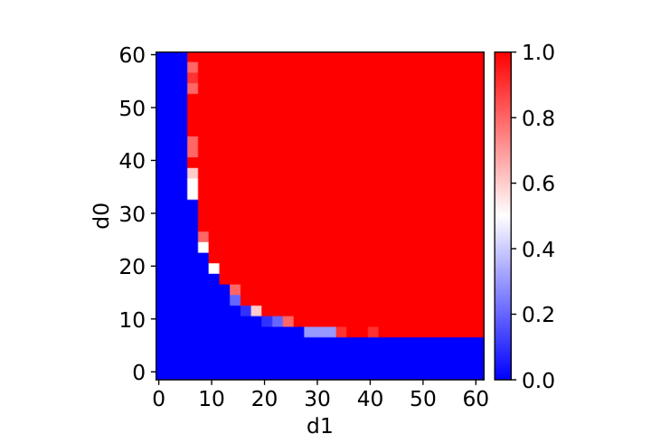
Refer to caption
(a) Probability of convergence, (W,V)(W,V) training
Refer to caption
(b) Avg. number of num. zeros in final preactivation, (W,V)(W,V) training
Refer to caption
(c) Avg. number of num. zeros in final preactivation, WW only
Figure 2. Numerical results for both training setups after 50​k50k SGD iterates.

We now turn to Figures 3 in which we analyze the training trajectories for both setups. It is seen that despite being close to global minima (loss is already close to 00 as seen on Figures 3(a), 3(f)), the number of numerical zeros in the preactivation pattern stays positive and is confined to a small range of values depending on the studied overparametrization level as presented on Figures 3(b), 3(g). This confirms the observation above that the GD scheme prefers minima located close to the boundaries between several ReLU activation patterns. In fact, these seem to be corner points connecting several regions. We are not aware of any explanation of such a phenomenon in the literature. Moreover, despite being close to global minima, the activation patterns keep changing while performing the consecutive GD iterates before eventually stabilizing in some region. At which iteration that happens, depends on the overparametrization level as presented on Figures 3(c), 3(h). This, in particular, demonstrates that most of the shallow ReLU networks training scheme happens in the nonlinear regime, i.e., it is not confined to a single ReLU activation region until the very end stage of training. The activation regions keep changing in a nonlinear fashion. Hence, the problem of studying the convergence of ReLU nets cannot be simplified to a study within a linear regime as suggested in Elkabetz and Cohen 2021.

Finally, on Figures 3(d), 3(i), 3(e), 3(j) we investigated the relative loss change Δ​ℒ=|ℒ⁡(θk)−ℒ⁡(θk−1)|ℒ⁡(θk−1)\Delta\mathcal{L}=\frac{|\mathcal{L}(\theta_{k})-\mathcal{L}(\theta_{k-1})|}{\mathcal{L}(\theta_{k-1})} and the relative differential change measured in the operator norm Δ​D=‖D​Yk−D​Yk−1‖o​p‖D​Yk−1‖o​p\Delta D=\frac{\|DY_{k}-DY_{k-1}\|_{op}}{\|DY_{k-1}\|_{op}}. It is visible that the relative differential change is by order of magnitude larger than the relative loss change, suggesting that the training for moderate and larger overparametrization levels is far from the lazy training regime studied in Chizat et al. 2019 characterized by Δ​ℒ≫Δ​D\Delta\mathcal{L}\gg\Delta D.

(a) Loss values
(b) Number of numerical zeros (threshold 1​e−081e-08) in the preactivation
(c) Hamming distance between ReLU indicators of consecutive iterates
(d) Δ​ℒ\Delta\mathcal{L}
(e) Δ​Y\Delta Y
(f) Loss values
(g) Number of numerical zeros
(h) Hamming distance between ReLU indicators of GD iterates
(i) Δ​ℒ\Delta\mathcal{L}
(j) Δ​Y\Delta Y
Figure 3. Top row: training the hidden layer of the shallow NN only. Bottom row: training both layers of the shallow NN. The number of the hidden neurons is varied (the NN configuration is provided in the legend) and the total number of epochs of the evolution is equal to 25​k25k. The solid curve presents the mean from five independent runs, and the shaded region presents the standard deviation, plotted every 100th epoch.

7. Conclusions and Future Work

We have demonstrated an improved trainability overparametrization bound of order Ω~​(N1.25)\tilde{\Omega}(N^{1.25}) on the hidden layer of shallow NN equipped with ReLU activation functions. We have obtained Theorem 5.6 – an result allowing to pass from continuous solutions of the DI to the dynamics of SGD. We believe that our contribution deepens the understanding of the optimization theory of NN. There are several natural directions of further research and we list some of them below. First direction is towards the theory of deep networks, where one could try to combine Theorem 5.6 with an analysis of DI dynamics in order to obtain improved overparametrization guarantees. Secondly, Theorem 5.6 might serve as a tool to obtain overparametrization bounds which are suggested by numerical experiments in Section 6. Finally, all known bounds for ReLU NNs are valid under strong, probabilistic data assumptions and it would be of interest to pursue directions of research that would allow for more general data such as in the case of smooth activations, cf. Table 1.

References

  • Allen-Zhu et al. (2019) Z. Allen-Zhu, Y. Li, and Z. Song. A convergence theory for deep learning via over-parameterization. In K. Chaudhuri and R. Salakhutdinov, editors, Proceedings of the 36th International Conference on Machine Learning, volume 97 of Proceedings of Machine Learning Research, pages 242–252. PMLR, 09–15 Jun 2019. URL https://proceedings.mlr.press/v97/allen-zhu19a.html.
  • Arora et al. (2019a) S. Arora, N. Cohen, N. Golowich, and W. Hu. A convergence analysis of gradient descent for deep linear neural networks. In International Conference on Learning Representations, 2019a. URL https://openreview.net/forum?id=SkMQg3C5K7.
  • Arora et al. (2019b) S. Arora, S. Du, W. Hu, Z. Li, and R. Wang. Fine-grained analysis of optimization and generalization for overparameterized two-layer neural networks. In K. Chaudhuri and R. Salakhutdinov, editors, Proceedings of the 36th International Conference on Machine Learning, volume 97 of Proceedings of Machine Learning Research, pages 322–332. PMLR, 09–15 Jun 2019b. URL https://proceedings.mlr.press/v97/arora19a.html.
  • Aubin and Cellina (2012) J.-P. Aubin and A. Cellina. Differential inclusions: set-valued maps and viability theory, volume 264. Springer Science & Business Media, 2012.
  • Auer et al. (1996a) P. Auer, M. Herbster, and M. K. Warmuth. Exponentially many local minima for single neurons. In D. S. Touretzky, M. C. Mozer, and M. E. Hasselmo, editors, Advances in Neural Information Processing Systems 8, pages 316–322. MIT Press, 1996a. URL http://papers.nips.cc/paper/1028-exponentially-many-local-minima-for-single-neurons.pdf.
  • Auer et al. (1996b) P. Auer, M. Herbster, and M. K. K. Warmuth. Exponentially many local minima for single neurons. In D. Touretzky, M. C. Mozer, and M. Hasselmo, editors, Advances in Neural Information Processing Systems, volume 8. MIT Press, 1996b. URL https://proceedings.neurips.cc/paper/1995/file/3806734b256c27e41ec2c6bffa26d9e7-Paper.pdf.
  • Baldi and Vershynin (2019) P. Baldi and R. Vershynin. The capacity of feedforward neural networks. Neural Networks, 116:288–311, 2019. ISSN 0893-6080. doi: https://doi.org/10.1016/j.neunet.2019.04.009. URL https://www.sciencedirect.com/science/article/pii/S0893608019301078.
  • Bianchi et al. (2022) P. Bianchi, W. Hachem, and S. Schechtman. Convergence of constant step stochastic gradient descent for non-smooth non-convex functions. Set-Valued and Variational Analysis, pages 1–31, 2022.
  • Brutzkus et al. (2018) A. Brutzkus, A. Globerson, E. Malach, and S. Shalev-Shwartz. SGD learns over-parameterized networks that provably generalize on linearly separable data. In International Conference on Learning Representations, 2018. URL https://openreview.net/forum?id=rJ33wwxRb.
  • Bubeck et al. (2020) S. Bubeck, R. Eldan, Y. T. Lee, and D. Mikulincer. Network size and size of the weights in memorization with two-layers neural networks. In H. Larochelle, M. Ranzato, R. Hadsell, M. Balcan, and H. Lin, editors, Advances in Neural Information Processing Systems 33: Annual Conference on Neural Information Processing Systems 2020, NeurIPS 2020, December 6-12, 2020, virtual, 2020. URL https://proceedings.neurips.cc/paper/2020/hash/34609bdc08a07ace4e1526bbb1777673-Abstract.html.
  • Chen et al. (2021) Z. Chen, Y. Cao, D. Zou, and Q. Gu. How much over-parameterization is sufficient to learn deep re{lu} networks? In International Conference on Learning Representations, 2021. URL https://openreview.net/forum?id=fgd7we_uZa6.
  • Chizat and Bach (2018) L. Chizat and F. Bach. On the global convergence of gradient descent for over-parameterized models using optimal transport. In S. Bengio, H. Wallach, H. Larochelle, K. Grauman, N. Cesa-Bianchi, and R. Garnett, editors, Advances in Neural Information Processing Systems, volume 31. Curran Associates, Inc., 2018. URL https://proceedings.neurips.cc/paper/2018/file/a1afc58c6ca9540d057299ec3016d726-Paper.pdf.
  • Chizat et al. (2019) L. Chizat, E. Oyallon, and F. Bach. On lazy training in differentiable programming. pages 2933–2943, 2019. URL http://papers.nips.cc/paper/8559-on-lazy-training-in-differentiable-programming.
  • Choromanska et al. (2015) A. Choromanska, M. Henaff, M. Mathieu, G. Ben Arous, and Y. LeCun. The Loss Surfaces of Multilayer Networks. In G. Lebanon and S. V. N. Vishwanathan, editors, Proceedings of the Eighteenth International Conference on Artificial Intelligence and Statistics, volume 38 of Proceedings of Machine Learning Research, pages 192–204, San Diego, California, USA, 09–12 May 2015. PMLR. URL https://proceedings.mlr.press/v38/choromanska15.html.
  • Clarke (1983) F. Clarke. Optimization and Nonsmooth Analysis. Wiley New York, 1983.
  • Cybenko (1989) G. Cybenko. Approximation by superpositions of a sigmoidal function. Mathematics of Control, Signals and Systems, 2(4):303–314, Dec 1989. ISSN 1435-568X. doi: 10.1007/BF02551274. URL https://doi.org/10.1007/BF02551274.
  • Davis et al. (2020) D. Davis, D. Drusvyatskiy, S. Kakade, and J. D. Lee. Stochastic subgradient method converges on tame functions. Found. Comput. Math., 20(1):119–154, 2020. ISSN 1615-3375. doi: 10.1007/s10208-018-09409-5. URL https://doi.org/10.1007/s10208-018-09409-5.
  • Dax (2013) A. Dax. From eigenvalues to singular values: a review. Advances in Pure Mathematics, 2013, 2013.
  • Du et al. (2019a) S. Du, J. Lee, H. Li, L. Wang, and X. Zhai. Gradient descent finds global minima of deep neural networks. In K. Chaudhuri and R. Salakhutdinov, editors, Proceedings of the 36th International Conference on Machine Learning, volume 97 of Proceedings of Machine Learning Research, pages 1675–1685. PMLR, 09–15 Jun 2019a. URL https://proceedings.mlr.press/v97/du19c.html.
  • Du et al. (2019b) S. S. Du, X. Zhai, B. Póczos, and A. Singh. Gradient descent provably optimizes over-parameterized neural networks. In 7th International Conference on Learning Representations, ICLR 2019, New Orleans, LA, USA, May 6-9, 2019. OpenReview.net, 2019b. URL https://openreview.net/forum?id=S1eK3i09YQ.
  • Elkabetz and Cohen (2021) O. Elkabetz and N. Cohen. Continuous vs. discrete optimization of deep neural networks. In Thirty-Fifth Conference on Neural Information Processing Systems, 2021. URL https://openreview.net/forum?id=iX0TSH45eOd.
  • Filippov (1988) A. F. Filippov. Differential equations with discontinuous righthand sides, volume 18 of Mathematics and its Applications (Soviet Series). Kluwer Academic Publishers Group, Dordrecht, 1988. ISBN 90-277-2699-X. doi: 10.1007/978-94-015-7793-9. URL https://doi.org/10.1007/978-94-015-7793-9. Translated from the Russian.
  • Hardt and Ma (2017) M. Hardt and T. Ma. Identity matters in deep learning. In 5th International Conference on Learning Representations, ICLR 2017, Toulon, France, April 24-26, 2017, Conference Track Proceedings. OpenReview.net, 2017. URL https://openreview.net/forum?id=ryxB0Rtxx.
  • Jacot et al. (2018) A. Jacot, F. Gabriel, and C. Hongler. Neural tangent kernel: Convergence and generalization in neural networks. In S. Bengio, H. Wallach, H. Larochelle, K. Grauman, N. Cesa-Bianchi, and R. Garnett, editors, Advances in Neural Information Processing Systems, volume 31. Curran Associates, Inc., 2018. URL https://proceedings.neurips.cc/paper/2018/file/5a4be1fa34e62bb8a6ec6b91d2462f5a-Paper.pdf.
  • Ji and Telgarsky (2020) Z. Ji and M. Telgarsky. Polylogarithmic width suffices for gradient descent to achieve arbitrarily small test error with shallow relu networks. In International Conference on Learning Representations, 2020. URL https://openreview.net/forum?id=HygegyrYwH.
  • Kawaguchi (2016) K. Kawaguchi. Deep learning without poor local minima. In D. Lee, M. Sugiyama, U. Luxburg, I. Guyon, and R. Garnett, editors, Advances in Neural Information Processing Systems, volume 29. Curran Associates, Inc., 2016. URL https://proceedings.neurips.cc/paper/2016/file/f2fc990265c712c49d51a18a32b39f0c-Paper.pdf.
  • Kawaguchi and Huang (2019) K. Kawaguchi and J. Huang. Gradient descent finds global minima for generalizable deep neural networks of practical sizes. In 57th Annual Allerton Conference on Communication, Control, and Computing, Allerton 2019, Monticello, IL, USA, September 24-27, 2019, pages 92–99. IEEE, 2019. doi: 10.1109/ALLERTON.2019.8919696. URL https://doi.org/10.1109/ALLERTON.2019.8919696.
  • Li et al. (2018) H. Li, Z. Xu, G. Taylor, C. Studer, and T. Goldstein. Visualizing the loss landscape of neural nets. In S. Bengio, H. Wallach, H. Larochelle, K. Grauman, N. Cesa-Bianchi, and R. Garnett, editors, Advances in Neural Information Processing Systems, volume 31. Curran Associates, Inc., 2018. URL https://proceedings.neurips.cc/paper/2018/file/a41b3bb3e6b050b6c9067c67f663b915-Paper.pdf.
  • Li and Liang (2018) Y. Li and Y. Liang. Learning overparameterized neural networks via stochastic gradient descent on structured data. In S. Bengio, H. M. Wallach, H. Larochelle, K. Grauman, N. Cesa-Bianchi, and R. Garnett, editors, Advances in Neural Information Processing Systems 31: Annual Conference on Neural Information Processing Systems 2018, NeurIPS 2018, December 3-8, 2018, Montréal, Canada, pages 8168–8177, 2018. URL https://proceedings.neurips.cc/paper/2018/hash/54fe976ba170c19ebae453679b362263-Abstract.html.
  • Liu et al. (2022) C. Liu, L. Zhu, and M. Belkin. Loss landscapes and optimization in over-parameterized non-linear systems and neural networks. Applied and Computational Harmonic Analysis, 2022. ISSN 1063-5203. doi: https://doi.org/10.1016/j.acha.2021.12.009. URL https://www.sciencedirect.com/science/article/pii/S106352032100110X.
  • Mei et al. (2018) S. Mei, A. Montanari, and P.-M. Nguyen. A mean field view of the landscape of two-layer neural networks. Proceedings of the National Academy of Sciences, 115(33):E7665–E7671, 2018. ISSN 0027-8424. doi: 10.1073/pnas.1806579115. URL https://www.pnas.org/content/115/33/E7665.
  • Nguyen (2021) Q. Nguyen. On the proof of global convergence of gradient descent for deep relu networks with linear widths. In M. Meila and T. Zhang, editors, Proceedings of the 38th International Conference on Machine Learning, volume 139 of Proceedings of Machine Learning Research, pages 8056–8062. PMLR, 18–24 Jul 2021. URL https://proceedings.mlr.press/v139/nguyen21a.html.
  • Nguyen and Hein (2018) Q. Nguyen and M. Hein. Optimization landscape and expressivity of deep cnns. In J. G. Dy and A. Krause, editors, Proceedings of the 35th International Conference on Machine Learning, ICML 2018, Stockholmsmässan, Stockholm, Sweden, July 10-15, 2018, volume 80 of Proceedings of Machine Learning Research, pages 3727–3736. PMLR, 2018. URL http://proceedings.mlr.press/v80/nguyen18a.html.
  • Nguyen et al. (2021) Q. Nguyen, M. Mondelli, and G. F. Montúfar. Tight bounds on the smallest eigenvalue of the neural tangent kernel for deep relu networks. In M. Meila and T. Zhang, editors, Proceedings of the 38th International Conference on Machine Learning, ICML 2021, 18-24 July 2021, Virtual Event, volume 139 of Proceedings of Machine Learning Research, pages 8119–8129. PMLR, 2021. URL http://proceedings.mlr.press/v139/nguyen21g.html.
  • Oymak and Soltanolkotabi (2020) S. Oymak and M. Soltanolkotabi. Toward moderate overparameterization: Global convergence guarantees for training shallow neural networks. IEEE J. Sel. Areas Inf. Theory, 1(1):84–105, 2020. doi: 10.1109/jsait.2020.2991332. URL https://doi.org/10.1109/jsait.2020.2991332.
  • Rockafellar and Wets (2009) R. T. Rockafellar and R. J.-B. Wets. Variational analysis, volume 317. Springer Science & Business Media, 2009.
  • Safran and Shamir (2018) I. Safran and O. Shamir. Spurious Local Minima are Common in Two-Layer ReLU Neural Networks. ICML 2018, 2018.
  • Shaham et al. (2018) U. Shaham, A. Cloninger, and R. R. Coifman. Provable approximation properties for deep neural networks. Applied and Computational Harmonic Analysis, 44(3):537–557, 2018. ISSN 1063-5203. doi: https://doi.org/10.1016/j.acha.2016.04.003. URL https://www.sciencedirect.com/science/article/pii/S1063520316300033.
  • Tropp (2012) J. A. Tropp. User-friendly tail bounds for sums of random matrices. Found. Comput. Math., 12(4):389–434, 2012. ISSN 1615-3375. doi: 10.1007/s10208-011-9099-z. URL https://doi.org/10.1007/s10208-011-9099-z.
  • Vershynin (2018) R. Vershynin. High-dimensional probability, volume 47 of Cambridge Series in Statistical and Probabilistic Mathematics. Cambridge University Press, Cambridge, 2018. ISBN 978-1-108-41519-4. doi: 10.1017/9781108231596. URL https://doi.org/10.1017/9781108231596. An introduction with applications in data science, With a foreword by Sara van de Geer.
  • Xie et al. (2017) B. Xie, Y. Liang, and L. Song. Diverse Neural Network Learns True Target Functions. In A. Singh and J. Zhu, editors, Proceedings of the 20th International Conference on Artificial Intelligence and Statistics, volume 54 of Proceedings of Machine Learning Research, pages 1216–1224, Fort Lauderdale, FL, USA, 20–22 Apr 2017. PMLR. URL http://proceedings.mlr.press/v54/xie17a.html.
  • Yun et al. (2019) C. Yun, S. Sra, and A. Jadbabaie. Small relu networks are powerful memorizers: a tight analysis of memorization capacity. In H. M. Wallach, H. Larochelle, A. Beygelzimer, F. d’Alché-Buc, E. B. Fox, and R. Garnett, editors, Advances in Neural Information Processing Systems 32: Annual Conference on Neural Information Processing Systems 2019, NeurIPS 2019, December 8-14, 2019, Vancouver, BC, Canada, pages 15532–15543, 2019. URL https://proceedings.neurips.cc/paper/2019/hash/dbea3d0e2a17c170c412c74273778159-Abstract.html.
  • Zhang et al. (2017) C. Zhang, S. Bengio, M. Hardt, B. Recht, and O. Vinyals. Understanding deep learning requires rethinking generalization. In 5th International Conference on Learning Representations, ICLR 2017, Toulon, France, April 24-26, 2017, Conference Track Proceedings. OpenReview.net, 2017. URL https://openreview.net/forum?id=Sy8gdB9xx.
  • Zou and Gu (2019) D. Zou and Q. Gu. An improved analysis of training over-parameterized deep neural networks. In H. M. Wallach, H. Larochelle, A. Beygelzimer, F. d’Alché-Buc, E. B. Fox, and R. Garnett, editors, Advances in Neural Information Processing Systems 32: Annual Conference on Neural Information Processing Systems 2019, NeurIPS 2019, December 8-14, 2019, Vancouver, BC, Canada, pages 2053–2062, 2019. URL https://proceedings.neurips.cc/paper/2019/hash/6a61d423d02a1c56250dc23ae7ff12f3-Abstract.html.

Appendix A Proof of Proposition 2.1

We begin with a standard result on the existence of local solutions to the DI (1), see, e.g., [Filippov 1988, pp. 77-78] for a detailed proof. We refer the interested reader also to Aubin and Cellina 2012 for a comprehensive treatment of the theory of DIs.

Theorem A.1 (Existence of local solutions).

If f:ℝd→ℝf\colon\mathbb{R}^{d}\to\mathbb{R} is locally Lipschitz, then there exists T>0T>0 and an arc xx such that the differential inclusion (1) is satisfied for almost every t∈[0,T)t\in[0,T). Moreover, for any bounded domain G∋x0G\ni x_{0}, each solution to (1) lying within GG can be continued up until it hits the boundary of GG.

Recall the definition of the chain rule 2. Its importance is shown in the following lemma.

Lemma A.2 (Davis et al. 2020).

If f:ℝd→ℝf\colon\mathbb{R}^{d}\to\mathbb{R} is locally Lipschitz, satisfies the chain rule (2) and x:ℝ+→ℝdx\colon\mathbb{R}_{+}\to\mathbb{R}^{d} is an arc satisfying the DI

x˙(t)∈−∂f(x(t))for a.e. t∈[0,T)\dot{x}(t)\in-\partial f(x(t))\quad\text{for a.e. }t\in[0,T)

for some T∈ℝ+∪{∞}T\in\mathbb{R}_{+}\cup\{\infty\}, then the equality ‖x˙​(t)‖=min⁡{‖v‖:v∈∂f⁡(x⁡(t))}=defm⁡(t)\|\dot{x}(t)\|=\min\{\,\|v\|\colon\;v\in\partial f(x(t))\,\}\stackrel{{\scriptstyle\mbox{\tiny{\raisebox{0.0pt}[0.0pt][0.0pt]{def}}}}}{{=}}m(t) holds for a.e. t∈[0,T)t\in[0,T) and in particular

f⁡(x⁡(t))=f⁡(x⁡(0))−∫0tm⁡(s)​𝑑sfor a.e. ​t∈[0,T).f(x(t))=f(x(0))-\int_{0}^{t}m(s)\,ds\quad\text{for a.e. }t\in[0,T).

Theorem A.1 and Lemma A.2 combined with the observation that the MSE loss function ℒ\mathcal{L} satisfies the chain rule (2), cf. Davis et al. 2020, immediately yield the following result.

Proposition A.3.

For any initial point θ0∈ℝD\theta_{0}\in\mathbb{R}^{D}, there exists T>0T>0 and a solution θ:[0,T)→ℝD\theta\colon[0,T)\to\mathbb{R}^{D} to the DI (3). Moreover, for any bounded domain G∋θ0G\ni\theta_{0}, each solution to (3) can be extended up until it hits the boundary of GG. Finally, for any such θ\theta,

(19) dd​t​ℒ​(θ⁡(t))≤−minv∈∂ℒ⁡(θ⁡(t))⁡‖v‖2for a.e. ​t∈[0,T).\frac{d}{dt}\mathcal{L}(\theta(t))\leq-\min_{v\in\partial\mathcal{L}(\theta(t))}\|v\|^{2}\quad\text{for a.e. }t\in[0,T).

Recall the definition of Clarke subdifferential operator,

(20) ∂f⁡(x)=defconv⁡{limn→∞∇f​(xn)for someDf∋xn​→n→∞​x}∀x∈ℝd,\partial f(x)\stackrel{{\scriptstyle\mbox{\tiny{\raisebox{0.0pt}[0.0pt][0.0pt]{def}}}}}{{=}}\conv\big\{\,\lim_{n\to\infty}\nabla f(x_{n})\quad\text{for some}\quad D_{f}\ni x_{n}\overset{n\to\infty}{\to}x\,\big\}\quad\forall\;x\in\mathbb{R}^{d},

where conv\conv is the convex hull operator. The Clarke subdifferential satisfies ∂f⁡(x)={∇f​(x)}\partial f(x)=\{\nabla f(x)\} for any x∈Dfx\in D_{f}. Recall also that for a matrix AA, we denote ii-th row vector of AA by Ai:A_{i:} and ii-th column vector of AA by A:iA_{:i} and that for a vector xx, dg⁡(x)\dg(x) denotes the diagonal matrix with xx on the diagonal.

Lemma below provides a description of ∂ℒ⁡(θ)\partial\mathcal{L}(\theta) for general θ∈ℝD\theta\in\mathbb{R}^{D} of a single hidden-layer NN.

Lemma A.4.

For any θ=(W,V)∈ℝD\theta=(W,V)\in\mathbb{R}^{D}, set Ri​j(θ)=Ri​j(Xi:W:j)R_{ij}(\theta)=R_{ij}(X_{i:}W_{:j}) to be generalized gradient of the function Xi:W:j↦ϕ(Xi:W:j)X_{i:}W_{:j}\mapsto\phi(X_{i:}W_{:j}). Then

(21) −∂W:jℒ(θ)\displaystyle-\partial_{W_{:j}}\mathcal{L}(\theta) ={XTdg(r:j)(Y−Y^)(Vj:)T:ri​j∈Ri​j for i∈[N]}for j∈[d1],\displaystyle=\big\{\,X^{T}\dg(r_{:j})(Y-\hat{Y})(V_{j:})^{T}\colon\;r_{ij}\in R_{ij}\text{ for }i\in[N]\,\big\}\quad\text{for }j\in[d_{1}],
(22) −∂Vℒ(θ)\displaystyle-\partial_{V}\mathcal{L}(\theta) ={HT​(Y−Y^)},\displaystyle=\big\{\,H^{T}(Y-\hat{Y})\,\big\},

where H=ϕ⁡(X​W)H=\phi(XW).

Proof.

The formulas are immediate at points where ℒ\mathcal{L} is differentiable, since in this case Clarke subdifferential coincides with the usual gradient. For points where ℒ\mathcal{L} is not differentiable, we apply the definition (20). ∎

Proposition A.5.

For any initial point θ0∈ℝD\theta_{0}\in\mathbb{R}^{D} and any solution θ:[0,T)→ℝD\theta\colon[0,T)\to\mathbb{R}^{D} to the DI (3), denote α0​(s)=defσm​i​n​(HT​(θ⁡(s)))\alpha_{0}(s)\stackrel{{\scriptstyle\mbox{\tiny{\raisebox{0.0pt}[0.0pt][0.0pt]{def}}}}}{{=}}\sigma_{min}(H^{T}(\theta(s))). Then

ℒ(θ(t))≤ℒ(θ(0))exp(−2∫0tα02(s)ds)for a.e. t∈[0,T).\mathcal{L}(\theta(t))\leq\mathcal{L}(\theta(0))\exp\big(-2\int_{0}^{t}\alpha_{0}^{2}(s)\,ds\big)\quad\text{for a.e. }t\in[0,T).
Proof.

By Lemma A.4, for any θ=(W,V)∈ℝD\theta=(W,V)\in\mathbb{R}^{D} and any v∈∂ℒ⁡(θ)v\in\partial\mathcal{L}(\theta) one has

∥v∥2≥minu∈−∂Vℒ(θ)∥u∥F2≥λm​i​n(HHT)∥(Y−Y^)∥F2.\|v\|^{2}\geq\min_{u\in-\partial_{V}\mathcal{L}(\theta)}\|u\|_{F}^{2}\geq\lambda_{min}(HH^{T})\|(Y-\hat{Y})\|_{F}^{2}.

Therefore, by an application of Proposition 2.1, dd​t​ℒ​(θ⁡(t))≤−2​α0​(t)​ℒ​(θ⁡(t))\frac{d}{dt}{\mathcal{L}}(\theta(t))\leq-2\alpha_{0}(t)\mathcal{L}(\theta(t)) for a.e. t∈[0,T)t\in[0,T). The result follows in virtue of Grönwall’s lemma. ∎

Finally, Proposition 2.1 is implied by Proposition A.3 and Proposition A.5 above.

Appendix B Proof of Lemma 3.1

Proof.

Observe that if v∈∂Wℒ⁡(θ′)v\in\partial_{W}\mathcal{L}(\theta^{\prime}) for some θ′=(W′,V′)∈ℝD\theta^{\prime}=(W^{\prime},V^{\prime})\in\mathbb{R}^{D}, then in virtue of Lemma A.4, v=XT​v~v=X^{T}\tilde{v} for some matrix v~\tilde{v} for which it holds that for some choice of the generalized gradient ri​j∈Ri​j​(θ′)r_{ij}\in R_{ij}(\theta^{\prime}), for each (i,j)∈[N]×[d1](i,j)\in[N]\times[d_{1}]

∥v~∥F2=∑j∈d1∥dg(r:j)(Y−ϕ(XW′)V′)(Vj:′)T∥F2≤∥(Y−ϕ(XW′)V′)∥F2∥V′∥F2,\|\tilde{v}\|_{F}^{2}=\sum_{j\in d_{1}}\|\dg(r_{:j})(Y-\phi(XW^{\prime})V^{\prime})(V^{\prime}_{j:})^{T}\|_{F}^{2}\leq\|(Y-\phi(XW^{\prime})V^{\prime})\|_{F}^{2}\|V^{\prime}\|_{F}^{2},

where we used Lemma H.1 and the fact that since ϕ\phi is 11-Lipschitz, then Ri​j⊂[−1,1]R_{ij}\subset[-1,1] and so ∥dg(r:j)∥o​p≤1\|\dg(r_{:j})\|_{op}\leq 1 for each j∈[d1]j\in[d_{1}]. Whence by Lemma H.1, ‖v‖F≤‖X‖o​p​‖Y−ϕ⁡(X​W′)​V′‖F​‖V′‖F\|v\|_{F}\leq\|X\|_{op}\|Y-\phi(XW^{\prime})V^{\prime}\|_{F}\|V^{\prime}\|_{F}.

Using the fact that θ\theta is a solution to DI (3), passing with the norm under the integral and using the above estimate on ‖v‖F\|v\|_{F}, we get that for any t∈[0,T)t\in[0,T)

(23) ‖W⁡(t)−W⁡(0)‖F=‖∫0tW˙​(s)​𝑑s‖F≤∫0t‖W˙​(s)‖F​𝑑s≤|X|∫0to​p⁡‖V⁡(s)‖F​2​ℒ​(θ⁡(s))​𝑑s=2​‖X‖o​p​(‖V⁡(0)‖F​ℒ¯​(t)+∫0t‖V⁡(s)−V⁡(0)‖F​ℒ⁡(θ⁡(s))​ds).\displaystyle\begin{split}\|W(t)-W(0)\|_{F}&=\Big\|\int_{0}^{t}\dot{W}(s)\,ds\Big\|_{F}\\ &\leq\int_{0}^{t}\|\dot{W}(s)\|_{F}\,ds\\ &\leq\|X\|_{op}\int_{0}^{t}\|V(s)\|_{F}\sqrt{2\mathcal{L}(\theta(s))}\,ds\\ &=\sqrt{2}\|X\|_{op}\Big(\|V(0)\|_{F}\bar{\mathcal{L}}(t)+\int_{0}^{t}\|V(s)-V(0)\|_{F}\sqrt{\mathcal{L}(\theta(s))}\,ds\Big).\end{split}

Similarly

(24) ‖V⁡(t)−V⁡(0)‖F=‖∫0tV˙​(s)​𝑑s‖F≤∫0t‖V˙​(s)‖F​𝑑s≤∫0t‖H⁡(s)‖F​‖Y−Y^​(s)‖F​𝑑s≤2​‖X‖o​p​(‖W⁡(0)‖F​ℒ¯​(t)+∫0t‖W⁡(s)−W⁡(0)‖F​ℒ⁡(θ⁡(s))​ds).\displaystyle\begin{split}\|V(t)-V(0)\|_{F}&=\Big\|\int_{0}^{t}\dot{V}(s)\,ds\Big\|_{F}\\ &\leq\int_{0}^{t}\|\dot{V}(s)\|_{F}\,ds\\ &\leq\int_{0}^{t}\|H(s)\|_{F}\|Y-\hat{Y}(s)\|_{F}\,ds\\ &\leq\sqrt{2}\|X\|_{op}\Big(\|W(0)\|_{F}\bar{\mathcal{L}}(t)+\int_{0}^{t}\|W(s)-W(0)\|_{F}\sqrt{\mathcal{L}(\theta(s))}\,ds\Big).\end{split}

Adding (24) to (23) and denoting Δ~​(s)=‖W⁡(t)−W⁡(0)‖F+‖V⁡(t)−V⁡(0)‖F\tilde{\Delta}(s)=\|W(t)-W(0)\|_{F}+\|V(t)-V(0)\|_{F} gives

Δ~​(t)≤2​‖X‖o​p​((‖W⁡(0)‖F+‖V⁡(0)‖F)​ℒ¯​(t)+∫0tΔ~​(s)​ℒ⁡(θ⁡(s))​𝑑s),\tilde{\Delta}(t)\leq\sqrt{2}\|X\|_{op}\Big(\big(\|W(0)\|_{F}+\|V(0)\|_{F}\big)\bar{\mathcal{L}}(t)+\int_{0}^{t}\tilde{\Delta}(s)\sqrt{\mathcal{L}(\theta(s))}\,ds\Big),

whence Grönwall’s lemma and the triangle inequality yield (5).

Let us turn to the proof of (6). Plugging (24) into (23) yields

(25) OPEN‖W⁡(t)−W⁡(0)‖F≤2​‖X‖o​p​‖V⁡(0)‖F​ℒ¯​(t))+2​‖X‖o​p2|W⁡(0)|∫0tF⁡ℒ¯​(s)​ℒ⁡(θ⁡(s))​𝑑s+2|X|∫0to​p2⁡ℒ⁡(θ⁡(s))​∫0s‖W⁡(u)−W⁡(0)‖F​ℒ⁡(θ⁡(u))​du​ds.\|W(t)-W(0)\|_{F}\leq\sqrt{2}\|X\|_{op}\|V(0)\|_{F}\bar{\mathcal{L}}(t))+2\|X\|_{op}^{2}\|W(0)\|_{F}\int_{0}^{t}\bar{\mathcal{L}}(s)\sqrt{\mathcal{L}(\theta(s))}\,ds\\ +2\|X\|_{op}^{2}\int_{0}^{t}\sqrt{\mathcal{L}(\theta(s))}\int_{0}^{s}\|W(u)-W(0)\|_{F}\sqrt{\mathcal{L}(\theta(u))}\,du\,ds.

Since for any function f:ℝ+→ℝf\colon\mathbb{R}_{+}\to\mathbb{R}, and any t≥0t\geq 0, by Fubini’s theorem

∫0tf⁡(s)​∫0sf⁡(u)​𝑑u​𝑑s=∫0t∫0tf⁡(s)​f​(u)​𝟏u≤s​𝑑u​𝑑s=12​(∫0tf⁡(s)​𝑑s)2,\int_{0}^{t}f(s)\int_{0}^{s}f(u)\,du\,ds=\int_{0}^{t}\int_{0}^{t}f(s)f(u){\bf 1}_{u\leq s}\,du\,ds=\frac{1}{2}\big(\int_{0}^{t}f(s)\,ds\big)^{2},

therefore

(26) ∫0tℒ¯​(s)​ℒ⁡(θ⁡(s))​𝑑s=12​(ℒ¯​(t))2.\int_{0}^{t}\bar{\mathcal{L}}(s)\sqrt{\mathcal{L}(\theta(s))}\,ds=\frac{1}{2}\big(\bar{\mathcal{L}}(t)\big)^{2}.

Similarly, we can estimate

(27) ∫0tℒ⁡(θ⁡(s))​∫0s‖W⁡(u)−W⁡(0)‖Fℒ⁡(θ⁡(u))​d​u​d​s≤∫0tℒ⁡(θ⁡(s))​𝑑s​∫0t‖W⁡(u)−W⁡(0)‖F​ℒ⁡(θ⁡(u))​𝑑u=ℒ¯​(t)⋅∫0t‖W⁡(s)−W⁡(0)‖F​ℒ⁡(θ⁡(s))​ds.\displaystyle\begin{split}\int_{0}^{t}\sqrt{\mathcal{L}(\theta(s))}\int_{0}^{s}\|W(u)-W(0)\|_{F}&\sqrt{\mathcal{L}(\theta(u))}\,du\,ds\\ &\leq\int_{0}^{t}\sqrt{\mathcal{L}(\theta(s))}\,ds\int_{0}^{t}\|W(u)-W(0)\|_{F}\sqrt{\mathcal{L}(\theta(u))}\,du\\ &=\bar{\mathcal{L}}(t)\cdot\int_{0}^{t}\|W(s)-W(0)\|_{F}\sqrt{\mathcal{L}(\theta(s))}\,ds.\end{split}

Denote Δ⁡(t)=‖W⁡(t)−W⁡(0)‖F/ℒ¯​(t)\Delta(t)=\|W(t)-W(0)\|_{F}/\bar{\mathcal{L}}(t). Estimating (25) with the use of (26) and (27), and dividing by ℒ¯​(t)\bar{\mathcal{L}}(t) results in

Δ⁡(t)≤2​‖X‖o​p​‖V⁡(0)‖F+‖X‖o​p2​‖W⁡(0)‖F​ℒ¯​(t)+2|X|∫0to​p2⁡Δ⁡(s)​ℒ¯​(s)​ℒ⁡(θ⁡(s))​𝑑s.\Delta(t)\leq\sqrt{2}\|X\|_{op}\|V(0)\|_{F}+\|X\|_{op}^{2}\|W(0)\|_{F}\bar{\mathcal{L}}(t)\\ +2\|X\|_{op}^{2}\int_{0}^{t}\Delta(s)\bar{\mathcal{L}}(s)\sqrt{\mathcal{L}(\theta(s))}\,ds.

Therefore, by Grönwall’s lemma

(28) Δ⁡(t)≤(2​‖X‖o​p​‖V⁡(0)‖F+‖X‖o​p2​‖W⁡(0)‖F​ℒ¯​(t))​exp⁡(2​‖X‖o​p2​∫0tℒ¯​(s)​ℒ⁡(θ⁡(s))​𝑑s).\Delta(t)\leq\Big(\sqrt{2}\|X\|_{op}\|V(0)\|_{F}+\|X\|_{op}^{2}\|W(0)\|_{F}\bar{\mathcal{L}}(t)\Big)\exp\Big(2\|X\|_{op}^{2}\int_{0}^{t}\bar{\mathcal{L}}(s)\sqrt{\mathcal{L}(\theta(s))}\,ds\Big).

The conclusion follows by multiplying (28) by ‖X‖o​p​ℒ¯​(t)\|X\|_{op}\bar{\mathcal{L}}(t) and using (26) in the exponent. ∎

Appendix C Proof of Theorem 4.3

Before we proceed to the proof of Theorem 4.3, we introduce the necessary notation and auxiliary facts. Since this theorem focuses on the properties of the initialization only, we write W=W0∈ℝd0×d1W=W_{0}\in\mathbb{R}^{d_{0}\times d_{1}}, α=α⁡(0)\alpha=\alpha(0) and H=ϕ⁡(X​W)H=\phi(XW) for short (so that α=σm​i​n​(HT)\alpha=\sigma_{min}(H^{T})). We introduce a random vector w∼𝒩⁡(0,Id0)w\sim\mathcal{N}(0,\Id_{d_{0}}) which is independent of X,WX,W, where Id0∈ℝd0×d0\Id_{d_{0}}\in\mathbb{R}^{d_{0}\times d_{0}} is the identity matrix. As XX, WW and ww are independent, we denote by 𝔼X\mathbb{E}_{X}, 𝔼W\mathbb{E}_{W} and 𝔼w\mathbb{E}_{w} the integration operators w.r.t. their respective laws. Finally, recall that ϕ\phi denotes the ReLU activation function and set

G⁡(X)=def𝔼w​[ϕ⁡(X​w)​ϕ​(X​w)T]andλ⁡(X)=defλm​i​n​(G⁡(X)).G(X)\stackrel{{\scriptstyle\mbox{\tiny{\raisebox{0.0pt}[0.0pt][0.0pt]{def}}}}}{{=}}\mathbb{E}_{w}[\phi(Xw)\phi(Xw)^{T}]\quad\text{and}\quad\lambda(X)\stackrel{{\scriptstyle\mbox{\tiny{\raisebox{0.0pt}[0.0pt][0.0pt]{def}}}}}{{=}}\lambda_{min}(G(X)).

Lemma C.1 below shows how to control α\alpha with λ⁡(X)\lambda(X) for a given matrix XX. We defer its proof until the end of this section.

Lemma C.1 (Lemma 5.2 in Nguyen et al. 2021).

There exist some absolute constant C>0C>0, s.t. for any Ψ:ℕ→[1,∞)\Psi\colon\mathbb{N}\to[1,\infty) and any X~∈ℝN×d0\tilde{X}\in\mathbb{R}^{N\times d_{0}} satisfying λ⁡(X~)>0\lambda(\tilde{X})>0, if

(29) d1≥max⁡(N,C​‖X~‖o​p2​(Ψ⁡(N)+log⁡(N))λ⁡(X~)⋅max⁡(1,log⁡(12​‖X~‖o​p2λ⁡(X~)))),d_{1}\geq\max\Big(N,C\frac{\|\tilde{X}\|_{op}^{2}(\Psi(N)+\log(N))}{\lambda(\tilde{X})}\cdot\max\Big(1,\log\big(\frac{12\|\tilde{X}\|_{op}^{2}}{\lambda(\tilde{X})}\big)\Big)\Big),

then

ℙ⁡(α>βw​d1​λ​(X)2|X=X~)≥1−exp⁡(−Ψ⁡(N)).\mathbb{P}\Big(\alpha>\frac{\beta_{w}\sqrt{d_{1}\lambda(X)}}{2}\;\Big|\;X=\tilde{X}\Big)\geq 1-\exp(-\Psi(N)).

One can choose C=16/(1−log⁡2)C=16/(1-\log 2).

For any two matrices A∈ℝnr×ncA\in\mathbb{R}^{n_{r}\times n_{c}}, B∈ℝnr×nc′B\in\mathbb{R}^{n_{r}\times n_{c}^{\prime}}, recall that their Khatri-Rao product is defined as

A∗B=def[A1:⊗B1:,…,Anr:⊗Bnr:]∈ℝnr×nc​nc′.A\ast B\stackrel{{\scriptstyle\mbox{\tiny{\raisebox{0.0pt}[0.0pt][0.0pt]{def}}}}}{{=}}[A_{1:}\otimes B_{1:},\ldots,A_{n_{r}:}\otimes B_{n_{r}:}]\in\mathbb{R}^{n_{r}\times n_{c}n_{c}^{\prime}}.

Moreover, recall that any function f:ℝ→ℝf\colon\mathbb{R}\to\mathbb{R}, s.t. 𝔼​[f2​(g)]<∞\mathbb{E}[f^{2}(g)]<\infty for g∼𝒩⁡(0,1)g\sim\mathcal{N}(0,1), admits the Hermite expansion, i.e.,

limn→∞𝔼​|f⁡(g)−∑k=0nμk​(f)​hk​(g)|2=0,\lim_{n\to\infty}\mathbb{E}\Big|f(g)-\sum_{k=0}^{n}\mu_{k}(f)h_{k}(g)\Big|^{2}=0,

where hkh_{k} is the kk-th probabilist’s Hermite polynomial, i.e.,

(30) hk(z)=(−1)kez2/2dkd​zke−z2/2,h_{k}(z)=(-1)^{k}e^{{z^{2}}/{2}}\frac{d^{k}}{dz^{k}}e^{-{z^{2}}/{2}},

h0≡1h_{0}\equiv 1 and μk​(f)\mu_{k}(f) is the kk-th Hermite coefficient given by

(31) μk​(f)=𝔼⁡[f⁡(g)​hk​(g)]𝔼​hk2​(g).\mu_{k}(f)=\frac{\mathbb{E}[f(g)h_{k}(g)]}{\sqrt{\mathbb{E}h_{k}^{2}(g)}}.

Lemma below follows from simple yet nontrivial calculations. Since we were unable to find its proof, we provide it for completeness.

Lemma C.2.

For any even positive integer kk,

(32) |μk​(ϕ)|2=Θ⁡(k−2.5).|\mu_{k}(\phi)|^{2}=\Theta(k^{-2.5}).
Proof.

We start with showing some properties of Hermite polynomials hkh_{k}. By (30), for any k∈ℕk\in\mathbb{N}

(33) hk′​(z)=z​hk​(z)−hk+1​(z).h_{k}^{\prime}(z)=zh_{k}(z)-h_{k+1}(z).

Moreover, by induction it also holds that

(34) hk′=k​hk−1h_{k}^{\prime}=kh_{k-1}

for k≥1k\geq 1. Indeed, the induction basis h1′=h0h_{1}^{\prime}=h_{0} is straightforward. Assume that for some k∈ℕk\in\mathbb{N}, hl′=l​hl−1h_{l}^{\prime}=lh_{l-1} for all l≤kl\leq k. Then, using (33), induction assumption and (33) again, we obtain that

hk+1′​(z)\displaystyle h_{k+1}^{\prime}(z) =(z​hk​(z)−hk′​(z))′\displaystyle=(zh_{k}(z)-h^{\prime}_{k}(z))^{\prime}
=hk​(z)+z​hk′​(z)−hk′′​(z)\displaystyle=h_{k}(z)+zh_{k}^{\prime}(z)-h_{k}^{\prime\prime}(z)
=hk​(z)+z​k​hk−1​(z)−k​hk−1′​(z)\displaystyle=h_{k}(z)+zkh_{k-1}(z)-kh_{k-1}^{\prime}(z)
=hk​(z)+k​hk​(z)\displaystyle=h_{k}(z)+kh_{k}(z)

as desired. Combining (33) and (34) we obtain for any k∈ℕ+k\in\mathbb{N}_{+},

(35) hk​(0)=−hk−1′​(0)=−(k−1)​hk−2​(0)={(−1)k/2​(k−1)!!if2|k,0else.h_{k}(0)=-h_{k-1}^{\prime}(0)=-(k-1)h_{k-2}(0)=\begin{cases}(-1)^{k/2}(k-1)!!&\text{if}\quad 2\,|\,k,\\ 0&\text{else}.\end{cases}

We not turn to the calculation of μk​(ϕ)\mu_{k}(\phi). Using integration by parts and (33) we obtain that for any k∈ℕ+k\in\mathbb{N}_{+},

∫0∞ze−z2/2hk(z)dz=−e−z2/2hk(z)|0∞+∫0∞e−z2/2hk′(z)dz=hk(0)+∫0∞e−z2/2hk′(z)dz=hk(0)+∫0∞e−z2/2(zhk(z)−hk+1(z))dz,\displaystyle\begin{split}\int_{0}^{\infty}ze^{-{z^{2}}/{2}}h_{k}(z)\,dz&=-e^{-z^{2}/2}h_{k}(z)\Big|_{0}^{\infty}+\int_{0}^{\infty}e^{-z^{2}/2}h_{k}^{\prime}(z)\,dz\\ &=h_{k}(0)+\int_{0}^{\infty}e^{-z^{2}/2}h_{k}^{\prime}(z)\,dz\\ &=h_{k}(0)+\int_{0}^{\infty}e^{-z^{2}/2}(zh_{k}(z)-h_{k+1}(z))\,dz,\end{split}

whence, after cancelling the same terms on both hand sides and using (35),

∫0∞e−z2/2hk+1(z)dz=hk(0)={(−1)k/2​(k−1)!!if2|k,0else.\int_{0}^{\infty}e^{-z^{2}/2}h_{k+1}(z)\,dz=h_{k}(0)=\begin{cases}(-1)^{k/2}(k-1)!!&\text{if}\quad 2\,|\,k,\\ 0&\text{else}.\end{cases}

Therefore,

(36) ∫0∞zdkd​zke−z2/2dz=zdk−1d​zk−1e−z2/2|0∞−∫0∞dk−1d​zk−1e−z2/2dz=ze−z/​2hk−1|0∞−∫0∞dk−1d​zk−1e−z2/2dz=−∫0∞dk−1d​zk−1e−z2/2dz=(−1)k∫0∞e−z2/2hk−1(z)dz={(−1)k−22​(k−3)!!if2|k,0else.\displaystyle\begin{split}\int_{0}^{\infty}z\frac{d^{k}}{dz^{k}}e^{-{z^{2}}/{2}}\,dz&=z\frac{d^{k-1}}{dz^{k-1}}e^{-{z^{2}}/{2}}\Big|_{0}^{\infty}-\int_{0}^{\infty}\frac{d^{k-1}}{dz^{k-1}}e^{-{z^{2}}/{2}}\,dz\\ &=ze^{-z^{/}2}h_{k-1}\Big|_{0}^{\infty}-\int_{0}^{\infty}\frac{d^{k-1}}{dz^{k-1}}e^{-{z^{2}}/{2}}\,dz\\ &=-\int_{0}^{\infty}\frac{d^{k-1}}{dz^{k-1}}e^{-{z^{2}}/{2}}\,dz\\ &=(-1)^{k}\int_{0}^{\infty}e^{-z^{2}/2}h_{k-1}(z)\,dz\\ &=\begin{cases}(-1)^{\frac{k-2}{2}}(k-3)!!&\text{if}\quad 2\,|\,k,\\ 0&\text{else.}\end{cases}\end{split}

Similarly, for any k≥1k\geq 1, by integration by parts and by (34),

(37) 𝔼​hk2​(g)=12​π∫ℝhk(z)(e−z2/2hk(z))dz=(−1)k2​π∫ℝhk(z)dkd​zke−z2/2dz=(−1)k2​π[hk(z)dk−1d​zk−1e−z2/2|−∞∞−∫ℝhk′(z)dk−1d​zk−1e−z2/2dz]=(−1)k−12​π∫ℝhk′(z)dk−1d​zk−1e−z2/2dz=k​𝔼​hk−12​(g)=k!.\displaystyle\begin{split}\mathbb{E}h_{k}^{2}(g)&=\frac{1}{\sqrt{2\pi}}\int_{\mathbb{R}}h_{k}(z)(e^{-z^{2}/2}h_{k}(z))\,dz\\ &=\frac{(-1)^{k}}{\sqrt{2\pi}}\int_{\mathbb{R}}h_{k}(z)\frac{d^{k}}{dz^{k}}e^{-z^{2}/2}\,dz\\ &=\frac{(-1)^{k}}{\sqrt{2\pi}}\Bigl[h_{k}(z)\frac{d^{k-1}}{dz^{k-1}}e^{-z^{2}/2}\,\Big|_{-\infty}^{\infty}-\int_{\mathbb{R}}h_{k}^{\prime}(z)\frac{d^{k-1}}{dz^{k-1}}e^{-z^{2}/2}\,dz\Bigr]\\ &=\frac{(-1)^{k-1}}{\sqrt{2\pi}}\int_{\mathbb{R}}h_{k}^{\prime}(z)\frac{d^{k-1}}{dz^{k-1}}e^{-z^{2}/2}\,dz\\ &=k\mathbb{E}h_{k-1}^{2}(g)\\ &=k!.\end{split}

Therefore, combining (36) and (37), we obtain for positive even kk,

μk​(ϕ)=𝔼​[hk​(g)​ϕ​(g)]𝔼​hk​(g)2=12​π​(−1)k−22​(k−3)!!k!.\displaystyle\begin{split}\mu_{k}(\phi)&=\frac{\mathbb{E}[h_{k}(g)\phi(g)]}{\sqrt{\mathbb{E}h_{k}(g)^{2}}}=\frac{1}{\sqrt{2\pi}}(-1)^{\frac{k-2}{2}}\frac{(k-3)!!}{\sqrt{k!}}.\end{split}

Using Stirling’s formula, one obtains that for such kk’s

(38) |μk​(ϕ)|2=Θ⁡(1k!⋅((k−2)!)2((k−2)!!)2)=Θ⁡(1k2⋅(k−2)!((k/2−1)!)2​2k−2)=Θ⁡(1k2⋅k−2​(k−2e)k−2(k/2−1)​(k−22​e)k−2​2k−2)=Θ⁡(k−2.5)\displaystyle\begin{split}|\mu_{k}(\phi)|^{2}&=\Theta\Big(\frac{1}{k!}\cdot\frac{((k-2)!)^{2}}{((k-2)!!)^{2}}\Big)\\ &=\Theta\Big(\frac{1}{k^{2}}\cdot\frac{(k-2)!}{((k/2-1)!)^{2}2^{k-2}}\Big)\\ &=\Theta\Big(\frac{1}{k^{2}}\cdot\frac{\sqrt{k-2}\bigl(\frac{k-2}{e}\bigr)^{k-2}}{(k/2-1)\bigl(\frac{k-2}{2e}\bigr)^{k-2}2^{k-2}}\Big)=\Theta(k^{-2.5})\end{split}

as desired. ∎

Lemma below provides an interpretable lower bound on λ⁡(X)\lambda(X) in terms of XX. We also defer its proof until the end of this section.

Lemma C.3 (Lemma 5.3 in Nguyen et al. 2021).

For any r∈ℕ+r\in\mathbb{N}_{+} and any non-zero X∈ℝN×d0X\in\mathbb{R}^{N\times d_{0}},

λ(X)≥[μr(ϕ)]2λm​i​n​((X∗r)​(X∗r)T)maxi∈N∥(X)i:∥22​(r−1).\lambda(X)\geq[\mu_{r}(\phi)]^{2}\frac{\lambda_{min}\big((X^{\ast r})(X^{\ast r})^{T}\big)}{\max_{i\in N}\|(X)_{i:}\|_{2}^{2(r-1)}.}

Recall that if a random vector z∈ℝz\in\mathbb{R} is sub-Gaussian, then there exists a constant σz\sigma_{z} depending on ‖z‖ψ2\|z\|_{\psi_{2}} only, s.t. for any 1-Lipschitz function f:ℝ→ℝf\colon\mathbb{R}\to\mathbb{R},

ℙ(z>𝔼f(z)+t)≤exp(−t2/σz2),\mathbb{P}(z>\mathbb{E}f(z)+t)\leq\exp\big(-{t^{2}}/{\sigma_{z}^{2}}\big),

cf. [Vershynin 2018, Proposition 2.5.2]. We are in position to prove Theorem 4.3.

Proof of Theorem 4.3.

By Gershgorin circle theorem, for any r∈ℕ+r\in\mathbb{N}_{+},

(39) λm​i​n​((X∗r)​(X∗r)T)≥mini∈[N]∥Xi:∥2​r−Nmaxi≠j|⟨Xi:,Xj:⟩|r=d0r−Nmaxi≠j|⟨Xi:,Xj:⟩|r.\displaystyle\begin{split}\lambda_{min}\big((X^{\ast r})(X^{\ast r})^{T}\big)&\geq\min_{i\in[N]}\|X_{i:}\|^{2r}-N\max_{i\neq j}|\langle X_{i:},X_{j:}\rangle|^{r}\\ &=d_{0}^{r}-N\max_{i\neq j}|\langle X_{i:},X_{j:}\rangle|^{r}.\end{split}

As for a fixed yy, ‖⟨x,y⟩‖ψ2≤‖y‖⋅‖x‖ψ2\|\langle x,y\rangle\|_{\psi_{2}}\leq\|y\|\cdot\|x\|_{\psi_{2}} and as ∥Xi:∥ψ2=𝒪(1)\|X_{i:}\|_{\psi_{2}}=\mathcal{O}(1) for i∈[N]i\in[N], then for for any i,j∈[N]i,j\in[N], i≠ji\neq j

ℙ(⟨Xi:,Xj:⟩>t)=𝔼[ℙ(⟨Xi:,Xj:⟩>t|Xj:)]≤exp(−t2σX2​d0),\displaystyle\mathbb{P}\Big(\langle X_{i:},X_{j:}\rangle>t\Big)=\mathbb{E}\Big[\mathbb{P}\Big(\langle X_{i:},X_{j:}\rangle>t\;\Big|\;X_{j:}\Big)\Big]\leq\exp\Big(-\frac{t^{2}}{\sigma_{X}^{2}d_{0}}\Big),

where σX>0\sigma_{X}>0 is some absolute constant dependent on supi∥Xi:∥ψ2=𝒪(1)\sup_{i}\|X_{i:}\|_{\psi_{2}}=\mathcal{O}(1) only. Therefore, by the union bound

(40) ℙ(⋂i≠j{|⟨Xi:,Xj:⟩|<t})≥1−N2exp(−t2σX2​d0).\displaystyle\mathbb{P}\Big(\bigcap_{i\neq j}\big\{|\langle X_{i:},X_{j:}\rangle|<t\big\}\Big)\geq 1-N^{2}\exp\Big(-\frac{t^{2}}{\sigma_{X}^{2}d_{0}}\Big).

Whence, by (39) and Lemma C.3,

λ⁡(X)≥[μr​(ϕ)]2​d0r−N​trd0r−1=[μr​(ϕ)]2​d0​(1−N​tr​d0−r)\lambda(X)\geq[\mu_{r}(\phi)]^{2}\frac{d_{0}^{r}-Nt^{r}}{d_{0}^{r-1}}=[\mu_{r}(\phi)]^{2}d_{0}\big(1-Nt^{r}d_{0}^{-r}\big)

holds with probability from (40) (at least).

Recall that by assumptions of Theorem 4.3, d0≥Nδ0d_{0}\geq N^{\delta_{0}} for some δ0∈(0,1)\delta_{0}\in(0,1). Choosing r=4​⌈1+δ0δ0⌉r=4\lceil\frac{1+\delta_{0}}{\delta_{0}}\rceil, and using Lemma C.2, reveals that [μr​(ϕ)]2=Ω⁡(δ02.5)[\mu_{r}(\phi)]^{2}=\Omega(\delta_{0}^{2.5}). Therefore, setting t=d03/4t=d_{0}^{3/4} yields that for some absolute constant c~>0\tilde{c}>0

λ(X)≥[μr(ϕ)]2d0(1−Nd0−r/4)≥[μr(ϕ)]2d0(1−N−δ0)≥c~d0δ02.5\displaystyle\lambda(X)\geq[\mu_{r}(\phi)]^{2}d_{0}\big(1-Nd_{0}^{-r/4}\big)\geq[\mu_{r}(\phi)]^{2}d_{0}\big(1-N^{-\delta_{0}}\big)\geq\tilde{c}d_{0}\delta_{0}^{2.5}

holds with probability at least 1−N2exp(−Nδ0/2/σX2)1-N^{2}\exp{(-N^{\delta_{0}/2}/\sigma_{X}^{2})}. Denote

A={λ(X)>c~d0δ02.5}∩{∥X∥o​p≤D​N}A=\{\,\lambda(X)>\tilde{c}d_{0}\delta_{0}^{2.5}\,\}\cap\{\,\|X\|_{op}\leq\sqrt{DN}\,\}

for some constant D>0D>0 big enough and s.t. for some absolute constant c>0c>0

ℙ(A)≥1−N2exp(−Nδ0/2/σX2)−exp(−cN),\mathbb{P}(A)\geq 1-N^{2}\exp(-N^{\delta_{0}/2}/\sigma_{X}^{2})-\exp(-cN),

which is possible in virtue of (40) and Lemma 4.4. By conditioning and using Lemma C.1, we get that

ℙ⁡(α>12​βw​d1​λ​(X))≥ℙ⁡(A)​(1−exp⁡(−Ψ⁡(N)))\mathbb{P}\Big(\alpha>\frac{1}{2}\beta_{w}\sqrt{d_{1}{\lambda}(X)}\Big)\geq\mathbb{P}(A)\big(1-\exp(-\Psi(N))\big)

for any function Ψ:ℕ→[1,∞)\Psi\colon\mathbb{N}\to[1,\infty) provided that

d1≥max⁡(N,C​N⁡(Ψ⁡(N)+log⁡(N))c~​d0​δ02.5⋅max⁡(1,log⁡(12​D​Nc~​d0​δ02.5)))d_{1}\geq\max\Big(N,C\frac{N(\Psi(N)+\log(N))}{\tilde{c}d_{0}\delta_{0}^{2.5}}\cdot\max\Big(1,\log\big(\frac{12DN}{\tilde{c}d_{0}\delta_{0}^{2.5}}\big)\Big)\Big)

for some (possibly different) absolute constant C>0C>0. We conclude by noting that

N​max⁡(1,C​(Ψ⁡(N)+log⁡(N))c~​d0​δ02.5⋅max⁡(1,log⁡(12​D​Nc~​d0​δ02.5)))≤N​max⁡(1,C​δ0−2.5​log⁡(1/δ0)​Ψ⁡(N)​log2​(N)d0)N\max\Big(1,C\frac{(\Psi(N)+\log(N))}{\tilde{c}d_{0}\delta_{0}^{2.5}}\cdot\max\Big(1,\log\big(\frac{12DN}{\tilde{c}d_{0}\delta_{0}^{2.5}}\big)\Big)\Big)\\ \leq N\max\Bigl(1,C\delta_{0}^{-2.5}\log(1/\delta_{0})\frac{\Psi(N)\log^{2}(N)}{d_{0}}\Bigr)

for some absolute constant C>0C>0 and estimating

ℙ⁡(A)​(1−exp⁡(−Ψ⁡(N)))\displaystyle\mathbb{P}(A)\big(1-\exp(-\Psi(N))\big) ≥1−N2exp(−Nδ0/2/σX2)−exp(−cN)−exp(−Ψ(N))\displaystyle\geq 1-N^{2}\exp{(-N^{\delta_{0}/2}/\sigma_{X}^{2})}-\exp(-cN)-\exp(-\Psi(N))
≥1−𝒪⁡(N2)​exp⁡(−Ω⁡(Nδ0/2))−exp⁡(−Ψ⁡(N)).\displaystyle\geq 1-\mathcal{O}(N^{2})\exp{(-\Omega(N^{\delta_{0}/2}))}-\exp(-\Psi(N)).

∎

We proceed with proofs of the remaining lemmas.

Proof of Lemma C.1.

Recall the definitions

G⁡(X)=def𝔼w​[ϕ⁡(X​w)​ϕ​(X​w)T],λ⁡(X)=defλm​i​n​(G⁡(X)),G(X)\stackrel{{\scriptstyle\mbox{\tiny{\raisebox{0.0pt}[0.0pt][0.0pt]{def}}}}}{{=}}\mathbb{E}_{w}[\phi(Xw)\phi(Xw)^{T}],\quad\lambda(X)\stackrel{{\scriptstyle\mbox{\tiny{\raisebox{0.0pt}[0.0pt][0.0pt]{def}}}}}{{=}}\lambda_{min}(G(X)),

where w∼𝒩⁡(0,Id0)w\sim\mathcal{N}(0,\Id_{d_{0}}) and introduce the following truncated versions of GG and λ\lambda for any t>0t>0

Gt​(X)=def𝔼w​[ϕ⁡(X​w)​ϕ​(X​w)T​𝟏‖ϕ⁡(X​w)‖≤t],λt​(X)=defλm​i​n​(Gt​(X)).G_{t}(X)\stackrel{{\scriptstyle\mbox{\tiny{\raisebox{0.0pt}[0.0pt][0.0pt]{def}}}}}{{=}}\mathbb{E}_{w}[\phi(Xw)\phi(Xw)^{T}{\bf 1}_{\|\phi(Xw)\|\leq t}],\quad\lambda_{t}(X)\stackrel{{\scriptstyle\mbox{\tiny{\raisebox{0.0pt}[0.0pt][0.0pt]{def}}}}}{{=}}\lambda_{min}(G_{t}(X)).

As the map w↦‖ϕ⁡(X​w)‖w\mapsto\|\phi(Xw)\| is ‖X‖o​p\|X\|_{op}-Lipschitz, then by Jensen’s inequality, integration by parts and by Gaussian concentration

‖Gt​(X)−G⁡(X)‖o​p\displaystyle\|G_{t}(X)-G(X)\|_{op} ≤𝔼w​‖ϕ⁡(X​w)​ϕ​(X​w)T​𝟏‖ϕ⁡(X​w)‖>t‖o​p\displaystyle\leq\mathbb{E}_{w}\big\|\phi(Xw)\phi(Xw)^{T}{\bf 1}_{\|\phi(Xw)\|>t}\big\|_{op}
=𝔼w​‖ϕ⁡(X​w)‖2​𝟏‖ϕ⁡(X​w)‖>t\displaystyle=\mathbb{E}_{w}\|\phi(Xw)\|^{2}{\bf 1}_{\|\phi(Xw)\|>t}
=∫0∞ℙ⁡(‖ϕ⁡(X​w)‖​𝟏‖ϕ⁡(X​w)‖>t≥s|X)​𝑑s\displaystyle=\int_{0}^{\infty}\mathbb{P}\big(\|\phi(Xw)\|{\bf 1}_{\|\phi(Xw)\|>t}\geq\sqrt{s}\;|\;X\big)\,ds
=∫0∞ℙ⁡(‖ϕ⁡(X​w)‖≥max⁡(s,t)|X)​𝑑s\displaystyle=\int_{0}^{\infty}\mathbb{P}\big(\|\phi(Xw)\|\geq\max(\sqrt{s},t)\;|\;X\big)\,ds
=t2​ℙ​(‖ϕ⁡(X​w)‖≥t|X)+∫t2∞ℙ⁡(‖ϕ⁡(X​w)‖≥s|X)​𝑑s\displaystyle=t^{2}\mathbb{P}\big(\|\phi(Xw)\|\geq t\;|\;X\big)+\int_{t^{2}}^{\infty}\mathbb{P}\big(\|\phi(Xw)\|\geq\sqrt{s}\;|\;X\big)\,ds
≤t2​exp⁡(−t22​‖X‖o​p2)+∫t2∞exp⁡(−s2​‖X‖o​p2)​𝑑s\displaystyle\leq t^{2}\exp\Big(\frac{-t^{2}}{2\|X\|_{op}^{2}}\Big)+\int_{t^{2}}^{\infty}\exp\Big(\frac{-s}{2\|X\|_{op}^{2}}\Big)\,ds
=(t2+2​‖X‖o​p2)​exp⁡(−t22​‖X‖o​p2)≤6​‖X‖o​p2​exp⁡(−t24​‖X‖o​p2),\displaystyle=\big(t^{2}+2\|X\|_{op}^{2}\big)\exp\Big(\frac{-t^{2}}{2\|X\|_{op}^{2}}\Big)\leq 6\|X\|_{op}^{2}\exp\Big(\frac{-t^{2}}{4\|X\|_{op}^{2}}\Big),

where in the last line we have used the inequality x≤exx\leq e^{x} valid for all x∈ℝx\in\mathbb{R}, with x=t2/4​‖X‖o​p2x=t^{2}/4\|X\|_{op}^{2}. Thus, for XX s.t. λ⁡(X)>0\lambda(X)>0, by choosing

(41) t2=4​‖X‖o​p2​max⁡(1,log⁡(12​‖X‖o​p2λ⁡(X))),t^{2}=4\|X\|_{op}^{2}\max\Big(1,\log\Big(\frac{12\|X\|_{op}^{2}}{\lambda(X)}\Big)\Big),

we get that ‖Gt​(X)−G⁡(X)‖o​p≤λ⁡(X)/2\|G_{t}(X)-G(X)\|_{op}\leq\lambda(X)/2, whence in virtue of Weyl’s inequality

(42) λt​(X)≥λ⁡(X)/2.\lambda_{t}(X)\geq\lambda(X)/2.

Define Ht∈ℝN×d1H_{t}\in\mathbb{R}^{N\times d_{1}} via (Ht):j=ϕ(XW:j)𝟏∥ϕ(XW:j)∥<tβw(H_{t})_{:j}=\phi(XW_{:j}){\bf 1}_{\|\phi(XW_{:j})\|<t\beta_{w}} for j∈[d1]j\in[d_{1}] and observe that HtHtT=∑j∈[d1](Ht):j(Ht):jTH_{t}H_{t}^{T}=\sum_{j\in[d_{1}]}(H_{t})_{:j}(H_{t})_{:j}^{T} and ∥(Ht):j(Ht):jT∥o​p=∥(Ht):j∥2≤βw2t2\|(H_{t})_{:j}(H_{t})_{:j}^{T}\|_{op}=\|(H_{t})_{:j}\|^{2}\leq\beta_{w}^{2}t^{2} for all j∈[d1]j\in[d_{1}]. By the matrix Chernoff inequality, cf. [Tropp 2012, Theorem 1.2], for any ε∈(0,1)\varepsilon\in(0,1)

(43) ℙ⁡(λm​i​n​(Ht​HtT)≤(1−ε)​λm​i​n​(𝔼W​[Ht​HtT])|X)≤N​[e−ε(1−ε)1−ε]λm​i​n​(𝔼W​[Ht​HtT])/βw2​t2.\mathbb{P}\Big(\lambda_{min}\big(H_{t}H_{t}^{T}\big)\leq(1-\varepsilon)\lambda_{min}\big(\mathbb{E}_{W}[H_{t}H^{T}_{t}]\big)\;\big|\;X\Big)\\ \leq N\Big[\frac{e^{-\varepsilon}}{(1-\varepsilon)^{1-\varepsilon}}\Big]^{\lambda_{min}\big(\mathbb{E}_{W}[H_{t}H^{T}_{t}]\big)/\beta_{w}^{2}t^{2}}.

Since for all j∈[d1]j\in[d_{1}], W:j∼𝒩(0,βwId0)W_{:j}\sim\mathcal{N}(0,\beta_{w}\Id_{d_{0}}), then

𝔼W​[Ht​HtT]\displaystyle\mathbb{E}_{W}[H_{t}H_{t}^{T}] =∑j∈[d1]𝔼W[(Ht):j(Ht):jT]\displaystyle=\sum_{j\in[d_{1}]}\mathbb{E}_{W}[(H_{t})_{:j}(H_{t})^{T}_{:j}]
=d1​𝔼w​[βw2​ϕ​(X​w)​ϕ​(X​w)T​𝟏‖βw​ϕ​(X​w)‖≤βw​t]=βw2​d1​Gt​(X).\displaystyle=d_{1}\mathbb{E}_{w}\big[\beta^{2}_{w}\phi(Xw)\phi(Xw)^{T}{\bf 1}_{\|\beta_{w}\phi(Xw)\|\leq\beta_{w}t}\big]=\beta_{w}^{2}d_{1}G_{t}(X).

Therefore, choosing ε=1/2\varepsilon=1/2 in (43), we obtain that

(44) ℙ⁡(λm​i​n​(Ht​HtT)≤12​βw2​d1​λt​(X)|X)≤exp⁡(−c​d1​λt​(X)t2+log⁡N)\mathbb{P}\Big(\lambda_{min}(H_{t}H_{t}^{T})\leq\frac{1}{2}\beta_{w}^{2}d_{1}\lambda_{t}(X)\;\big|\;X\Big)\leq\exp\Big(-c\frac{d_{1}\lambda_{t}(X)}{t^{2}}+\log N\Big)

for any t≥0t\geq 0, where c=12​(1−log⁡2)c=\frac{1}{2}(1-\log 2).

Finally, noting that α2=λm​i​n​(H​HT)≥λm​i​n​(Ht​HtT)\alpha^{2}=\lambda_{min}(HH^{T})\geq\lambda_{min}(H_{t}H_{t}^{T}) and combining this observations with (42) and (44), we get that for any X~\tilde{X} s.t. λ⁡(X~)>0\lambda(\tilde{X})>0,

ℙ⁡(α≥12​βw​d1​λ​(X)|X=X~)>1−exp⁡(−c​d1​λ​(X~)2​t~2+log⁡N)\mathbb{P}\Big(\alpha\geq\frac{1}{2}\beta_{w}\sqrt{d_{1}\lambda(X)}\;|\;X=\tilde{X}\Big)>1-\exp\Big(-c\frac{d_{1}\lambda(\tilde{X})}{2\tilde{t}^{2}}+\log N\Big)

for t~2=4​‖X~‖o​p2​max⁡(1,log⁡(12​‖X~‖o​p2λ⁡(X~)))\tilde{t}^{2}=4\|\tilde{X}\|_{op}^{2}\max\big(1,\log\big(\frac{12\|\tilde{X}\|_{op}^{2}}{\lambda(\tilde{X})}\big)\big). The conclusion follows as by (29)

−c​d1​λ​(X~)2​t~2+log⁡N=−c​d1​λ​(X~)4​‖X~‖o​p2​max⁡(1,log⁡(12​‖X~‖o​p2λ⁡(X~)))+log⁡N≤−Ψ⁡(N).\displaystyle-c\frac{d_{1}\lambda(\tilde{X})}{2\tilde{t}^{2}}+\log N=\frac{-cd_{1}\lambda(\tilde{X})}{4\|\tilde{X}\|_{op}^{2}\max\Big(1,\log\Big(\frac{12\|\tilde{X}\|_{op}^{2}}{\lambda(\tilde{X})}\Big)\Big)}+\log N\leq-\Psi(N).

∎

Proof of Lemma C.3.

Denote J=dg(∥X1:∥,…,∥XN:∥)J=\dg\big(\|X_{1:}\|,\ldots,\|X_{N:}\|\big) and F=J−1​XF=J^{-1}X. Using the fact that for g,g′∼𝒩⁡(0,1)g,g^{\prime}\sim\mathcal{N}(0,1) and any k,l∈ℕk,l\in\mathbb{N}, we get that for any (i,j)∈[N]×[d1](i,j)\in[N]\times[d_{1}]

J−1​G​(X)i​j​J−1\displaystyle J^{-1}G(X)_{ij}J^{-1} =𝔼w[ϕ(⟨Fi:,w⟩)ϕ(⟨Fj:,w⟩)]\displaystyle=\mathbb{E}_{w}\big[\phi(\langle F_{i:},w\rangle)\phi(\langle F_{j:},w\rangle)\big]
=limn→∞𝔼w[∑k=0nμk(ϕ)hk(⟨Fi:,w⟩)∑l=0nμl(ϕ)hl(⟨Fj:,w⟩)]\displaystyle=\lim_{n\to\infty}\mathbb{E}_{w}\Big[\sum_{k=0}^{n}\mu_{k}(\phi)h_{k}(\langle F_{i:},w\rangle)\sum_{l=0}^{n}\mu_{l}(\phi)h_{l}(\langle F_{j:},w\rangle)\Big]
=limn→∞∑k,l=0nμk(ϕ)μl(ϕ)𝔼w[hk(⟨Fi:,w⟩)hl(⟨Fj:,w⟩)]\displaystyle=\lim_{n\to\infty}\sum_{k,l=0}^{n}\mu_{k}(\phi)\mu_{l}(\phi)\mathbb{E}_{w}\Big[h_{k}(\langle F_{i:},w\rangle)h_{l}(\langle F_{j:},w\rangle)\Big]
=limn→∞∑k=0n[μk(ϕ)]2⟨Fi:,Fj:⟩k=∑k=0∞[μk(ϕ)]2⟨(F∗k)i:,(F∗k)j:⟩.\displaystyle=\lim_{n\to\infty}\sum_{k=0}^{n}[\mu_{k}(\phi)]^{2}\langle F_{i:},F_{j:}\rangle^{k}=\sum_{k=0}^{\infty}[\mu_{k}(\phi)]^{2}\big\langle(F^{\ast k})_{i:},(F^{\ast k})_{j:}\big\rangle.

Therefore, for a fixed r∈ℕ+r\in\mathbb{N}_{+},

λ⁡(X)\displaystyle\lambda(X) =λm​i​n​(J⁡[∑k=0∞[μk​(ϕ)]2​(F∗k)​(F∗k)T]​J)\displaystyle=\lambda_{min}\Big(J\Big[\sum_{k=0}^{\infty}[\mu_{k}(\phi)]^{2}(F^{\ast k})(F^{\ast k})^{T}\Big]J\Big)
≥[μr​(ϕ)]2​λm​i​n​(J⁡(F∗r)​(F∗r)T​J)\displaystyle\geq[\mu_{r}(\phi)]^{2}\lambda_{min}\Big(J(F^{\ast r})(F^{\ast r})^{T}J\Big)
=[μr​(ϕ)]2​λm​i​n​(J−(r−1)​(X∗r)​(X∗r)T​J−(r−1))\displaystyle=[\mu_{r}(\phi)]^{2}\lambda_{min}\Big(J^{-(r-1)}(X^{\ast r})(X^{\ast r})^{T}J^{-(r-1)}\Big)
≥[μr​(ϕ)]2​λm​i​n​((X∗r)​(X∗r)T)maxi∈[N]⁡(Ji​i)2​(r−1)\displaystyle\geq[\mu_{r}(\phi)]^{2}\frac{\lambda_{min}\big((X^{\ast r})(X^{\ast r})^{T}\big)}{\max_{i\in[N]}(J_{ii})^{2(r-1)}}

as desired. ∎

Appendix D Proof of Lemma 4.4

Proof.

The concentration results for W0W_{0}, V0V_{0} and XX are standard, cf [Vershynin 2018, Theorems 3.1.1, 4.6.1].

We turn to the concentration result for ℒ\mathcal{L}. Let us write V=V0V=V_{0} and W=W0W=W_{0} for short. Since ℒ⁡(θ0)≤2​‖Y‖F2+2​‖Y^‖F2\mathcal{L}(\theta_{0})\leq 2\|Y\|_{F}^{2}+2\|\hat{Y}\|_{F}^{2}, then it suffices to estimate ‖Y^‖F=‖ϕ⁡(X​W)​V‖F\|\hat{Y}\|_{F}=\|\phi(XW)V\|_{F}.

As for any A∈ℝN×d1A\in\mathbb{R}^{N\times d_{1}}, the function ℝd1×d2∋V↦‖A​V‖F\mathbb{R}^{d_{1}\times d_{2}}\ni V\mapsto\|AV\|_{F} is ‖A‖F\|A\|_{F}-Lipschitz with respect to the Frobenius norm on ℝd1×d2\mathbb{R}^{d_{1}\times d_{2}}, then Gaussian concentration applied to VV yields

(45) ℙ(∥AV∥F≤𝔼∥AV∥F+t)≥1−exp(−t2/2βv2∥A∥F2)∀t≥0.\mathbb{P}\big(\|AV\|_{F}\leq\mathbb{E}\|AV\|_{F}+t\big)\geq 1-\exp\big(-t^{2}/2\beta_{v}^{2}\|A\|^{2}_{F}\big)\quad\forall\;t\geq 0.

By independence of the entries of VV, 𝔼⟨v,V:j⟩2=βv2∥v∥2\mathbb{E}\langle v,V_{:j}\rangle^{2}=\beta_{v}^{2}\|v\|^{2} for any v∈ℝd1v\in\mathbb{R}^{d_{1}} and j∈[d2]j\in[d_{2}]. Using this fact and Jensen’s inequality we get that

𝔼​‖A​V‖F≤𝔼​‖A​V‖F2\displaystyle\mathbb{E}\|AV\|_{F}\leq\sqrt{\mathbb{E}\|AV\|_{F}^{2}} =(∑i∈[N],j∈[d2]𝔼(Ai:V:j)2)1/2\displaystyle=\Big(\sum_{i\in[N],j\in[d_{2}]}\mathbb{E}(A_{i:}V_{:j})^{2}\Big)^{1/2}
=(∑i∈[N],j∈[d2]βv2∥Ai:∥2)1/2=βvd2∥A∥F,\displaystyle=\Big(\sum_{i\in[N],j\in[d_{2}]}\beta_{v}^{2}\|A_{i:}\|^{2}\Big)^{1/2}=\beta_{v}\sqrt{d_{2}}\|A\|_{F},

whence (45) with A=ϕ⁡(X​W)A=\phi(XW), t=d2​βv​‖A‖F​log⁡(N)t=\sqrt{d_{2}}\beta_{v}\|A\|_{F}\sqrt{\log(N)} and conditioned on the variables XX, WW, implies that

‖Y^‖F≤2​βv​d2​log⁡(N)​‖ϕ⁡(X​W)‖F\|\hat{Y}\|_{F}\leq 2\beta_{v}\sqrt{d_{2}\log(N)}\|\phi(XW)\|_{F}

with probability at least 1−exp(−d2log(N)/2)1-\exp(-d_{2}\log(N)/2). Estimating ‖ϕ⁡(X​W)‖F≤‖X​W‖F≤‖X‖o​p​‖W‖F\|\phi(XW)\|_{F}\leq\|XW\|_{F}\leq\|X\|_{op}\|W\|_{F} yields the desired estimate for ℒ\mathcal{L}. ∎

Appendix E Proof of Corollary 4.5

Proof.

As Nδ0≤d0≤NN^{\delta_{0}}\leq d_{0}\leq N, then by Lemma 4.4

∥W0∥F=Θ(βwd0​d1),∥V0∥F=Θ(βvd1​d2),∥X∥o​p=𝒪(N),and\displaystyle\|W_{0}\|_{F}=\Theta(\beta_{w}\sqrt{d_{0}d_{1}}),\quad\|V_{0}\|_{F}=\Theta(\beta_{v}\sqrt{d_{1}d_{2}}),\quad\|X\|_{op}=\mathcal{O}(\sqrt{N}),\quad\text{and}
ℒ⁡(θ0)=𝒪⁡(N​log⁡(N)⋅d0​d1​d2​βv2​βw2)\displaystyle\mathcal{L}(\theta_{0})=\mathcal{O}(N\log(N)\cdot d_{0}d_{1}d_{2}\beta_{v}^{2}\beta_{w}^{2})

with probability at least

1−2​exp⁡(−Ω⁡(d0​d1))−2​exp⁡(−Ω⁡(d1​d2))−exp⁡(−Ω⁡(N))−exp⁡(−Ω⁡(d2​log⁡(N))).1-2\exp(-\Omega(d_{0}d_{1}))-2\exp(-\Omega(d_{1}d_{2}))-\exp(-\Omega(N))-\exp(-\Omega(d_{2}\log(N))).

Using Theorem 4.3 with

Ψ⁡(N)=d0N⋅[d2​N2.5d0​βw2]1/(ρ+1)\Psi(N)=\frac{d_{0}}{N}\cdot\Big[\frac{d_{2}N^{2.5}}{d_{0}\beta_{w}^{2}}\Big]^{1/{(\rho+1)}}

yields

F⁡(θ0,X,Y)\displaystyle F(\theta_{0},X,Y) =(2​2​ℒ⁡(θ0)​‖X‖o​p2​‖V0‖Fα03​(0)+2​ℒ⁡(θ0)​‖X‖o​p3​‖W0‖Fα05​(0))​exp⁡(4​‖X‖o​p2​ℒ​(θ0)α04​(0))\displaystyle=\Big(2\sqrt{2}\frac{\sqrt{\mathcal{L}(\theta_{0})}\|X\|_{op}^{2}\|V_{0}\|_{F}}{\alpha_{0}^{3}(0)}+2\frac{\mathcal{L}(\theta_{0})\|X\|_{op}^{3}\|W_{0}\|_{F}}{\alpha_{0}^{5}(0)}\Big)\exp\Big(\frac{4\|X\|^{2}_{op}\mathcal{L}(\theta_{0})}{\alpha_{0}^{4}(0)}\Big)
=𝒪⁡(N​N​log⁡N​d0​d1​d2​βw​βv2d01.5​d11.5​βw3+N2.5​log⁡(N)​d01.5​d11.5​d2​βw3​βv2d02.5​d12.5​βw5)​exp⁡(𝒪⁡(N2​log⁡N​d0​d1​d2​βw2​βv2d02​d12​βw4))\displaystyle=\mathcal{O}\Big(\frac{N\sqrt{N\log N}\sqrt{d_{0}}d_{1}d_{2}\beta_{w}\beta_{v}^{2}}{d_{0}^{1.5}d_{1}^{1.5}\beta_{w}^{3}}+\frac{N^{2.5}\log(N)d_{0}^{1.5}d_{1}^{1.5}d_{2}\beta_{w}^{3}\beta_{v}^{2}}{d_{0}^{2.5}d_{1}^{2.5}\beta_{w}^{5}}\Big)\exp\Big(\mathcal{O}\big(\frac{N^{2}\log Nd_{0}d_{1}d_{2}\beta^{2}_{w}\beta^{2}_{v}}{d^{2}_{0}d^{2}_{1}\beta_{w}^{4}}\big)\Big)
=𝒪⁡(d2​N​N​log⁡N​βv2d0​d1​βw2+d2​N2.5​log⁡(N)​βv2d0​d1​βw2)​exp⁡(𝒪⁡(d2​N2​log⁡N​βv2d0​d1​βw2))\displaystyle=\mathcal{O}\Big(\frac{d_{2}N\sqrt{N\log N}\beta_{v}^{2}}{d_{0}\sqrt{d_{1}}\beta_{w}^{2}}+\frac{d_{2}N^{2.5}\log(N)\beta_{v}^{2}}{d_{0}d_{1}\beta_{w}^{2}}\Big)\exp\Big(\mathcal{O}\big(\frac{d_{2}N^{2}\log N\beta^{2}_{v}}{d_{0}d_{1}\beta^{2}_{w}}\big)\Big)
=𝒪⁡(d2​N2.5​log⁡(N)​βv2d0​d1​βw2)​exp⁡(𝒪⁡(d2​N2​log⁡N​βv2d0​d1​βw2))\displaystyle=\mathcal{O}\Big(\frac{d_{2}N^{2.5}\log(N)\beta_{v}^{2}}{d_{0}d_{1}\beta_{w}^{2}}\Big)\exp\Big(\mathcal{O}\big(\frac{d_{2}N^{2}\log N\beta^{2}_{v}}{d_{0}d_{1}\beta^{2}_{w}}\big)\Big)
=𝒪⁡(1d11+ρ⋅d2​N2.5​log⁡(N)d0​βw2)​exp⁡(𝒪⁡(1d11+ρ⋅d2​N2​log⁡Nd0​βw2))\displaystyle=\mathcal{O}\Big(\frac{1}{d_{1}^{1+\rho}}\cdot\frac{d_{2}N^{2.5}\log(N)}{d_{0}\beta_{w}^{2}}\Big)\exp\Big(\mathcal{O}\Big(\frac{1}{d_{1}^{1+\rho}}\cdot\frac{d_{2}N^{2}\log N}{d_{0}\beta^{2}_{w}}\Big)\Big)
=𝒪⁡(1log⁡N)​exp⁡(𝒪⁡(1N​(log⁡N)1+2​ρ))\displaystyle=\mathcal{O}\Big(\frac{1}{\log N}\Big)\exp\Big(\mathcal{O}\Big(\frac{1}{\sqrt{N}(\log N)^{1+2\rho}}\Big)\Big)

with probability at least 1−exp(−d0N⋅[d2​N2.5d0​βw2]1/(ρ+1))−𝒪(N2)exp(−Ω(Nδ0/2))−exp(−Ω(d2logN))=o(1).1-\exp\big(-\frac{d_{0}}{N}\cdot\big[\frac{d_{2}N^{2.5}}{d_{0}\beta_{w}^{2}}\big]^{1/{(\rho+1)}}\big)-\mathcal{O}(N^{2})\exp(-\Omega(N^{\delta_{0}/2}))-\exp(-\Omega(d_{2}\log N))=o(1). – we use tha fact that δ0≤1\delta_{0}\leq 1 together with the probability bound of Theorem 4.3. The result follows in virtue of Theorem 3.4. ∎

Appendix F Proof of Theorem 5.6

Proof.

Let l=supθ∈Qℒ~​(θ)l=\sup_{\theta\in Q}\tilde{\mathcal{L}}(\theta) and

T∗=inf{t≥0:l​e−γ​t≤ε/2}=max⁡(0,log⁡(2​l/ε)γ)T^{\ast}=\inf\{\,t\geq 0\colon le^{-\gamma t}\leq\varepsilon/2\,\}=\max\left(0,\frac{\log(2l/\varepsilon)}{\gamma}\right)

so that all solutions to the DI (18) initialized in the set QQ fall to ℒ~−1​([0,ε/2])\tilde{\mathcal{L}}^{-1}([0,\varepsilon/2]) before time T∗T^{\ast} (and clearly never escapes it). For any r>0r>0, let Gr=G+B⁡(0,r)G_{r}=G+B(0,r) be the rr-widening of GG and denote

L=defsup{∥v∥:v∈∂ℒ~(θ),θ∈G1}.L\stackrel{{\scriptstyle\mbox{\tiny{\raisebox{0.0pt}[0.0pt][0.0pt]{def}}}}}{{=}}\sup\{\,\|v\|\colon v\in\partial\tilde{\mathcal{L}}(\theta),\;\theta\in G_{1}\,\}.

As G1G_{1} is compact and ℒ~\tilde{\mathcal{L}} is locally Lipschitz, then L<∞L<\infty. Choose Δ=min⁡(ε/2​L,1)\Delta=\min(\varepsilon/2L,1) and let ζ:ℝD→[0,1]\zeta\colon\mathbb{R}^{D}\to[0,1] be a smooth function such that ζ|GΔ≡1\zeta_{|G_{\Delta}}\equiv 1 and ζ|(G2​Δ)c≡0\zeta_{|(G_{2\Delta})^{c}}\equiv 0. Finally, for any θ∈ℝD\theta\in\mathbb{R}^{D} and A∈[N](b)A\in[N]^{(b)}, let f⁡(θ,A)=ℒ~b​(θ,A)⋅ζ⁡(θ)f(\theta,A)=\tilde{\mathcal{L}}^{b}(\theta,A)\cdot\zeta(\theta) and note that for θ∈GΔ\theta\in G_{\Delta}, 𝔼​f​(θ,Ab)=bN​ℒ~​(θ)\mathbb{E}f(\theta,A_{b})=\frac{b}{N}\tilde{\mathcal{L}}(\theta), where Ab∼Unif⁡([N]b)A_{b}\sim\operatorname{Unif}([N]^{b}).

Further, for any η>0\eta>0, let τη=inf{k∈ℕ+:θkη∉GΔ}\tau^{\eta}=\inf\{k\in\mathbb{N}_{+}\colon\theta^{\eta}_{k}\notin G_{\Delta}\} and set χkη=θkη\chi_{k}^{\eta}=\theta_{k}^{\eta} for k∈[τη]k\in[\tau^{\eta}] (note that τη\tau^{\eta} is a random variable measurable w.r.t. the sigma field generated by θ0,ξ1,ξ2,…\theta_{0},\xi_{1},\xi_{2},\ldots) and χkη\chi^{\eta}_{k} for k>τηk>\tau^{\eta} to be arbitrary such that χkη∈−η∂f(χk−1η,ξk)\chi^{\eta}_{k}\in-\eta\partial f(\chi^{\eta}_{k-1},\xi_{k}), where θkη\theta^{\eta}_{k} is the ℒ~b\tilde{\mathcal{L}}^{b}-SGD sequence belonging to the family given in the statement of the theorem. Since for any A∈[N]bA\in[N]^{b}, (f(⋅,A))|GΔ=(ℒ~b(⋅,A))|GΔ(f(\cdot,A))_{|G_{\Delta}}=(\tilde{\mathcal{L}}^{b}(\cdot,A))_{|G_{\Delta}}, then (χkη)k∈ℕ(\chi^{\eta}_{k})_{k\in\mathbb{N}} is indeed an ff-SGD sequence. Additionally, by construction (χkη)k∈ℕ(\chi_{k}^{\eta})_{k\in\mathbb{N}} escapes the set GΔG_{\Delta} if and only if (θkη)k∈ℕ(\theta_{k}^{\eta})_{k\in\mathbb{N}} does so.

As for any A∈[N](b)A\in[N]^{(b)}, f⁡(⋅,A)f(\cdot,A) is locally Lipschitz and compactly supported, then it is Lipschitz with some constant LA<∞L_{A}<\infty. Therefore ff satisfies assumption 1 of Theorem 5.5 with κ⁡(⋅,A)≡LA\kappa(\cdot,A)\equiv L_{A}. Assumptions 2 and 3 of Theorem 5.5 also hold since the underlying probability space [N](b)[N]^{(b)} is finite. Finally, assumption 4 follows as well immediately from the definition of ℒ~b\tilde{\mathcal{L}}^{b}, local smoothness of ζ\zeta and assumptions on ℒ~i\tilde{\mathcal{L}}_{i} for i∈[N]i\in[N]. We, therefore, apply Theorem 5.5 with 𝒦=Q\mathcal{K}=Q, T=1+Nb​T∗T=1+\frac{N}{b}T^{\ast} and ε~=Δ\tilde{\varepsilon}=\Delta. As a result, the DI problem associated with ff,

(46) χ˙(t)∈−∂𝔼f(χ(t),Ab)for a.e. t∈[0,T]\dot{\chi}(t)\in-\partial\mathbb{E}f(\chi(t),A_{b})\quad\text{for a.e. }t\in[0,T]

is well-defined. Moreover, for δ>0\delta>0, there exists η0≤1\eta_{0}\leq 1 such that for a.e. η∈(0,η0)\eta\in(0,\eta_{0}) and for any family of ff-SGD sequences 𝒮={(χkη)k∈ℕ:η>0}\mathcal{S}=\{\,(\chi_{k}^{\eta})_{k\in\mathbb{N}}\colon\eta>0\,\} defined above,

(47) ℙ(∃χ:[0,T]→ℝD solving (46) s.t. χ(0)∈Qandsupt∈[0,T]|χ(t)−χ¯η(t)|<Δ|θ0∈Q)≥1−δ,\mathbb{P}\Big(\exists\;\chi\colon[0,T]\to\mathbb{R}^{D}\text{ solving~\eqref{eq:DI_sgd_f} s.t. }\chi(0)\in Q\;\text{and}\;\sup_{t\in[0,T]}|\chi(t)-\bar{\chi}^{\eta}(t)|<\Delta\;\Big|\;\theta_{0}\in Q\Big)\geq 1-\delta,

where χ¯η​(t)\bar{\chi}^{\eta}(t) is the piecewise interpolated process associated with some (χkη)k∈ℕ∈𝒮(\chi_{k}^{\eta})_{k\in\mathbb{N}}\in\mathcal{S} via (17) (note that χ¯η\bar{\chi}^{\eta} is in fact a random variable measurable w.r.t. θ0,ξ1,ξ2,…\theta_{0},\xi_{1},\xi_{2},\ldots).

Using the fact that (𝔼f(⋅,Ab))|GΔ=(bNℒ~(⋅))|GΔ(\mathbb{E}f(\cdot,A_{b}))_{|G_{\Delta}}=(\frac{b}{N}\tilde{\mathcal{L}}(\cdot))_{|G_{\Delta}}, we infer that if χ:[0,T]→ℝD\chi\colon[0,T]\to\mathbb{R}^{D} solves (46), χ⁡(0)∈Q\chi(0)\in Q and τ=inf{t≥0:χ⁡(t)∉GΔ}\tau=\inf\{t\geq 0\colon\chi(t)\notin G_{\Delta}\}, then θ⁡(t)=defχ⁡(Nb​t)\theta(t)\stackrel{{\scriptstyle\mbox{\tiny{\raisebox{0.0pt}[0.0pt][0.0pt]{def}}}}}{{=}}\chi(\frac{N}{b}t) solves the DI

θ˙(t)∈−∂ℒ~(θ(t))for a.e.t∈[0,bτ/N].\dot{\theta}(t)\in-\partial\tilde{\mathcal{L}}(\theta(t))\quad\text{for a.e.}\quad t\in[0,b\tau/N].

Since any θ\theta initialized in QQ does not escape the set GG by assumption and since GG lies in the interior of GΔG_{\Delta}, then τ=T\tau=T, i.e., χ\chi remains in GG.

Figure 4. Illustration of the sets and flows that appear in the proof of Theorem 5.6

Let η∈(0,η0)\eta\in(0,\eta_{0}), θ0∈Q\theta_{0}\in Q be such that there exists χ:[0,T]→ℝD\chi\colon[0,T]\to\mathbb{R}^{D} initialized in QQ, which is Δ\Delta close to the (truncated) piecewise affine interpolated process χ¯η:[0,T]→ℝD\bar{\chi}^{\eta}\colon[0,T]\to\mathbb{R}^{D} associated with (χkη)k∈ℕ(\chi_{k}^{\eta})_{k\in\mathbb{N}} defined above (with the initial condition χ0η=θ0\chi_{0}^{\eta}=\theta_{0}). By (47), this happens with probability at least 1−δ1-\delta. By the discussion above, such χ\chi never escapes the set GG, whence χ¯η\bar{\chi}^{\eta} remains in the set GΔG_{\Delta}. As a consequence, denoting k∗=⌊Tη⌋k^{\ast}=\lfloor\frac{T}{\eta}\rfloor to be maximal index such that χk∗η\chi_{k^{\ast}}^{\eta} lies on the curve χ¯η:[0,T]→ℝD\bar{\chi}^{\eta}\colon[0,T]\to\mathbb{R}^{D}, we infer that χkη\chi_{k}^{\eta} also remains in GΔG_{\Delta} for all k∈[k∗]k\in[k^{\ast}] and therefore τη>k∗\tau^{\eta}>k^{\ast}, which by definition implies that χkη=θkη\chi_{k}^{\eta}=\theta_{k}^{\eta} for all k∈[k∗]k\in[k^{\ast}].

Combining all the above observations, we deduce that with probability at least 1−δ1-\delta, conditioned on a value of θ0∈Q\theta_{0}\in Q, for a.e. η∈(0,η0)\eta\in(0,\eta_{0}) and k∗=⌊Tη⌋k^{\ast}=\lfloor\frac{T}{\eta}\rfloor

ℒ~​(θk∗η)=ℒ~​(χk∗η)\displaystyle\tilde{\mathcal{L}}(\theta_{k^{\ast}}^{\eta})=\tilde{\mathcal{L}}\left(\chi_{k^{\ast}}^{\eta}\right) =ℒ~​(χ¯η​(η​k∗))\displaystyle=\tilde{\mathcal{L}}\left(\bar{\chi}^{\eta}\left(\eta k^{\ast}\right)\right)
≤ℒ~(χ(ηk∗))+sup{∥v∥:v∈∂f(x),x∈GΔ}⋅|χ(ηk∗)−χ¯(ηk∗)|\displaystyle\leq\tilde{\mathcal{L}}\left(\chi\left(\eta k^{\ast}\right)\right)+\sup\{\,\|v\|\colon v\in\partial f(x),\;x\in G_{\Delta}\,\}\cdot|\chi(\eta k^{\ast})-\bar{\chi}(\eta k^{\ast})|
=ℒ~(θ(η​bN⌊N​T∗b​η+1η⌋))+sup{∥v∥:v∈∂f(x),x∈GΔ}⋅|χ(ηk)−χ¯(ηk)|\displaystyle=\tilde{\mathcal{L}}\Big(\theta\Big(\frac{\eta b}{N}\Big\lfloor\frac{NT^{\ast}}{b\eta}+\frac{1}{\eta}\Big\rfloor\Big)\Big)+\sup\{\,\|v\|\colon v\in\partial f(x),\;x\in G_{\Delta}\,\}\cdot|\chi(\eta k)-\bar{\chi}(\eta k)|
≤ε2+L​Δ≤ε\displaystyle\leq\frac{\varepsilon}{2}+L\Delta\leq\varepsilon

as desired. ∎

Appendix G Training hidden layer only

In this section, we apply the theory designed in the prequel to the setting in which only the first weight matrix WW is being updated using GD (whereas the second VV is fixed to some specific values). This is the training setup, which was introduced in Oymak and Soltanolkotabi 2020. We combine the results from Oymak and Soltanolkotabi 2020 with our technique which results in a simpler approach as compared to the original one for showing overparametrization in such a training setup. However, the order of overparametrization that we obtain by proceeding is slightly off compared to the original work.

Consider the model with output dimension d2=1d_{2}=1, i.e.,

ℝN×d0∋X↦y^=defϕ⁡(X​W)​v∈ℝN,\mathbb{R}^{N\times d_{0}}\ni X\mapsto\hat{y}\stackrel{{\scriptstyle\mbox{\tiny{\raisebox{0.0pt}[0.0pt][0.0pt]{def}}}}}{{=}}\phi(XW)v\in\mathbb{R}^{N},

where X∈ℝd0×d1X\in\mathbb{R}^{d_{0}\times d_{1}}, W∈ℝd0×d1W\in\mathbb{R}^{d_{0}\times d_{1}}, v∈ℝd1v\in\mathbb{R}^{d_{1}}. In the sequel, we work under the following assumptions on the data and initialization, which are the same as in Oymak and Soltanolkotabi 2020.

Assumption G.1.

Matrix XX has i.i.d. rows from the uniform distribution on the unit sphere in ℝd0\mathbb{R}^{d_{0}}. The output vector yy is such that |yi|=𝒪⁡(1)|y_{i}|=\mathcal{O}(1) for all ii, so that ‖y‖2=𝒪⁡(N)\|y\|_{2}=\mathcal{O}(\sqrt{N}). Vector vv is initialized s.t. half of its entries are ‖y‖2/N​d1\|y\|_{2}/\sqrt{Nd_{1}} and the other half is set to −∥y∥2/N​d1-\|y\|_{2}/\sqrt{Nd_{1}}. Weight matrix WW has i.i.d. 𝒩⁡(0,1)\mathcal{N}(0,1) entries.

We restrict our attention to the case, where only WW is trained and vv remains fixed, i.e., we have ℒ=ℒ⁡(W)\mathcal{L}=\mathcal{L}(W) and we consider the following DI problem

(48) dd​sW(s)=−∂ℒ(W)for a.e. s∈ℝ+.\frac{d}{ds}W(s)=-\partial\mathcal{L}(W)\quad\text{for a.e. }s\in\mathbb{R}_{+}.

The following theorem is the main result of this section.

Theorem G.2.

Let the data satisfy Assumption G.1. Assume that

(49) d0∈[N,N],d1≥C⁡(max⁡(N​log⁡Nd0,N5d04))d_{0}\in[\sqrt{N},N],\quad d_{1}\geq C\Bigl(\max\bigl(\frac{N\log N}{d_{0}},\frac{N^{5}}{d_{0}^{4}}\bigr)\Bigr)

for some absolute constant C≥0C\geq 0. Then WHP any solution WW to the DI (48) can be extended to a solution on ℝ+\mathbb{R}_{+} and any such extension satisfies ℒ⁡(W⁡(t))≤ℒ⁡(W⁡(0))​exp⁡(−c​t​β02)\mathcal{L}(W(t))\leq\mathcal{L}(W(0))\exp(-ct\beta_{0}^{2}) for some absolute c>0c>0.

Using Theorem 5.6, we immediately obtain the following corollary to SGD iterates.

Corollary G.3.

Under the assumptions of Theorem G.2, choose error ε>0\varepsilon>0, batch size b=b⁡(N)b=b(N) and any family {(Wkη):η>0}\{(W_{k}^{\eta})\colon\eta>0\} of ℒb\mathcal{L}^{b}-SGD sequences (14). Then, WHP there exists a step size η0∈(0,1)\eta_{0}\in(0,1), s.t. for a.e. η∈(0,η0)\eta\in(0,\eta_{0}), ℒ⁡(Wk∗η)<ε\mathcal{L}(W^{\eta}_{k^{\ast}})<\varepsilon for sufficiently large k∗k^{\ast}.

The proof of Theorem G.2 is presented at the end of this section and is an adaptation of the reasoning presented in Section 4 together with some ideas from Oymak and Soltanolkotabi 2020, presented below.

In the case of training one layer only, one has

∂ℒ⁡(W)=XT​dg⁡(y^−y)​ϕ′​(W​X)​dg⁡(v),\displaystyle\partial\mathcal{L}(W)=X^{T}\dg(\hat{y}-y)\phi^{\prime}(WX)\dg(v),

where ϕ′​(W​X)i​j\phi^{\prime}(WX)_{ij} for (i,j)∈[d0]×[d1](i,j)\in[d_{0}]\times[d_{1}] is the Clark subdifferential of Wi:X:j↦ϕ(Wi:X:j)W_{i:}X_{:j}\mapsto\phi(W_{i:}X_{:j}) and ϕ′​(W​X)=⨂i​jϕ′​(W​X)i​j\phi^{\prime}(WX)=\bigotimes_{ij}\phi^{\prime}(WX)_{ij}. Let Rs∈ϕ′​(X​W​(s))R_{s}\in\phi^{\prime}(XW(s)) be such that W˙​(s)=XT​dg⁡(y^​(s)−y)​Rs​dg⁡(v)\dot{W}(s)=X^{T}\dg(\hat{y}(s)-y)R_{s}\dg(v) for a.e. ss.

For a vector x=(x1,…,xd)∈ℝdx=(x_{1},\ldots,x_{d})\in\mathbb{R}^{d} and integer m∈{1,…,d}m\in\{1,\ldots,d\}, let ‖x‖m−\|x\|_{m-} denote mm-th smallest entry of |x|=(|x1|,…,|xd|)|x|=(|x_{1}|,\ldots,|x_{d}|).

Lemma G.4 (Lemma C.2 in Oymak and Soltanolkotabi 2020).

If

∥Ws−W0∥F≤mmini∈[N]∥Xi:W0∥m−,\|W_{s}-W_{0}\|_{F}\leq\sqrt{m}\min_{i\in[N]}\|X_{i:}W_{0}\|_{m-},

then maxi∈[N]∥(Rs−R0)i:∥2≤2​m\max_{i\in[N]}\|(R_{s}-R_{0})_{i:}\|_{2}\leq\sqrt{2m}.

Lemma G.5 (Lemma C.3 in Oymak and Soltanolkotabi 2020).

If ∥Xi:∥2=1\|X_{i:}\|_{2}=1 for all ii and W0∈ℝd0×d1W_{0}\in\mathbb{R}^{d_{0}\times d_{1}} has i.i.d. 𝒩⁡(0,1)\mathcal{N}(0,1) entries, then

mini∈[N]∥Xi:W0∥m−≥m2​d1for all i=1,2,…,N\min_{i\in[N]}\|X_{i:}W_{0}\|_{m-}\geq\frac{m}{2d_{1}}\quad\text{for all }i=1,2,\ldots,N

with probability at least 1−Ne−m/61-Ne^{-m/6} for any m∈{1,2,…,d1}m\in\{1,2,\ldots,d_{1}\}.

Corollary G.6.

If ∥Xi:∥2=1\|X_{i:}\|_{2}=1 for all ii and W0∈ℝd0×d1W_{0}\in\mathbb{R}^{d_{0}\times d_{1}} has i.i.d. 𝒩⁡(0,1)\mathcal{N}(0,1) entries, then

maxi∈[N]∥(Rs−R0)i:∥2≤10log⁡N+2(d1∥Ws−W0∥F)1/3\max_{i\in[N]}\|(R_{s}-R_{0})_{i:}\|_{2}\leq 10\sqrt{{\log N}}+2(d_{1}\|W_{s}-W_{0}\|_{F})^{1/3}

for all ss with probability at least 1−1N1-\frac{1}{N}.

Proof.

Note that maxi∥(Rs−R0)i:∥≤d1\max_{i}\|(R_{s}-R_{0})_{i:}\|\leq\sqrt{d_{1}} always. Therefore, by Lemma G.4 and Lemma G.5, if ‖Ws−W0‖F≤m​m/2​d1\|W_{s}-W_{0}\|_{F}\leq m\sqrt{m}/2d_{1}, then maxi∈[N]∥(Rs−R0)i:∥2≤2​m\max_{i\in[N]}\|(R_{s}-R_{0})_{i:}\|_{2}\leq\sqrt{2m} with probability at least 1−Ne−min(m,d1)/61-Ne^{-\min(m,d_{1})/6} for any m∈ℕm\in\mathbb{N}. Pick

m=⌈12​log⁡N+(2​d1​‖Ws−W0‖F)2/3⌉m=\lceil 12\log N+(2d_{1}\|W_{s}-W_{0}\|_{F})^{2/3}\rceil

so that ‖Ws−W0‖F≤m​m/2​d1\|W_{s}-W_{0}\|_{F}\leq m\sqrt{m}/2d_{1}. As d1≥Nd_{1}\geq N (this is our global assumption) and

⌈a+log⁡N⌉≤a+log⁡N+1≤a+4​log⁡N\lceil a+\log N\rceil\leq a+\log N+1\leq a+4\log N

for 2≤N∈ℕ2\leq N\in\mathbb{N} and any a>0a>0, then

12​log⁡N≤m≤48​log⁡N+(2​d1​‖Ws−W0‖F)2/3.12\log N\leq m\leq 48\log N+(2d_{1}\|W_{s}-W_{0}\|_{F})^{2/3}.

Therefore, using sub-additivity of the square root we get that

maxi∥(Rs−R0)i:∥2≤2​m≤10log⁡N+2(d1∥Ws−W0∥F)1/3\max_{i}\|(R_{s}-R_{0})_{i:}\|_{2}\leq\sqrt{2m}\leq 10\sqrt{\log N}+2(d_{1}\|W_{s}-W_{0}\|_{F})^{1/3}

with probability at least 1−Ne−min(m,d1)/6≥1−Ne−2​log⁡N=1−1N1-Ne^{-\min(m,d_{1})/6}\geq 1-Ne^{-2\log N}=1-\frac{1}{N}, as desired. ∎

Proposition G.7.

Denote β0=defσm​i​n​((X⋆(R0​dg⁡(v)))T)\beta_{0}\stackrel{{\scriptstyle\mbox{\tiny{\raisebox{0.0pt}[0.0pt][0.0pt]{def}}}}}{{=}}\sigma_{min}((X\star(R_{0}\dg(v)))^{T}). If

d0∈[N,N]andd1≥max⁡(N,C⁡(N​log⁡N)/d0),d_{0}\in[\sqrt{N},N]\quad\text{and}\quad d_{1}\geq\max(N,C(N\log N)/d_{0}),

then

c​‖y‖N≤β0≤C​‖y‖2d0c\frac{\|y\|}{\sqrt{N}}\leq\beta_{0}\leq C\frac{\|y\|_{2}}{\sqrt{d_{0}}}

WHP for some absolute constants c,C>0c,C>0.

Proof.

To get the first estimate, apply [Oymak and Soltanolkotabi 2020, Lemma 6.7] and note that ‖v‖2=d1​‖v‖∞\|v\|_{2}=\sqrt{d_{1}}\|v\|_{\infty} and that for the uniform distribution on the unit sphere, ‖X‖o​p≲N/d0\|X\|_{op}\lesssim\sqrt{N/d_{0}} and λ⁡(X)∼const\lambda(X)\sim\operatorname{const} (note that β0=σm​i​n​(𝒥⁡(W0))\beta_{0}=\sigma_{min}(\mathcal{J}(W_{0})) in their notation). The second estimate follows from Weyl’s inequality, cf. [Oymak and Soltanolkotabi 2020, Lemma 6.6]. ∎

Proof of Theorem G.2.

For any WW, we have

minw∈∂L⁡(W)⁡‖w‖F2\displaystyle\min_{w\in\partial L(W)}\|w\|_{F}^{2} =minR∈ϕ′​(X​W)⁡‖(X⋆(R​dg⁡(v)))T​(y^−y)‖22\displaystyle=\min_{R\in\phi^{\prime}(XW)}\|(X\star(R\dg(v)))^{T}(\hat{y}-y)\|_{2}^{2}
≥2​ℒ​(W)⋅minR∈ϕ′​(X​W)⁡σm​i​n2​((X⋆(R​dg⁡(v)))T),\displaystyle\geq 2\mathcal{L}(W)\cdot\min_{R\in\phi^{\prime}(XW)}\sigma_{min}^{2}((X\star(R\dg(v)))^{T}),

where in the first equality we have used Lemma H.2 below with A=XTA=X^{T}, x=y^−yx=\hat{y}-y and B=R​dg⁡(v)B=R\dg(v). Denote βs=defσm​i​n​((X⋆(Rs​dg⁡(v)))T)\beta_{s}\stackrel{{\scriptstyle\mbox{\tiny{\raisebox{0.0pt}[0.0pt][0.0pt]{def}}}}}{{=}}\sigma_{min}((X\star(R_{s}\dg(v)))^{T}) and write ℒ⁡(t)=defℒ⁡(W⁡(t))\mathcal{L}(t)\stackrel{{\scriptstyle\mbox{\tiny{\raisebox{0.0pt}[0.0pt][0.0pt]{def}}}}}{{=}}\mathcal{L}(W(t)) for short. Then, by Proposition 2.1 and Grönwall’s lemma

(50) ℒ(t)≤ℒ(0)exp(−2∫0tβs2ds)≤ℒ(0)exp(−2tβ02+4β0∫0t|βs−β0|ds).\displaystyle\begin{split}\mathcal{L}(t)\leq\mathcal{L}(0)\exp\bigl(-2\int_{0}^{t}\beta_{s}^{2}\,ds\bigr)\leq\mathcal{L}(0)\exp\bigl(-2t\beta_{0}^{2}+4\beta_{0}\int_{0}^{t}|\beta_{s}-\beta_{0}|\,ds\bigr).\end{split}

By Weyl’s inequality, Lemma H.2 applied with A=XTA=X^{T} and B=(Rs−R0)​dg⁡(v)B=(R_{s}-R_{0})\dg(v) and by Corollary G.6 we get

(51) |βs−β0|≤‖(X⋆((Rs−R0)​dg⁡(v)))T‖o​p=supx:‖x‖2=1∥(X⋆((Rs−R0)dg(v)))Tx∥2≤∥X∥o​pmaxi∈[N]∥vi(Rs−R0)i:∥2≤∥X∥o​p∥v∥∞maxi∈[N]∥(Rs−R0)i:∥2≤‖X‖o​p​‖v‖∞​[10​log⁡N+2​(d1​‖Ws−W0‖F)1/3],\displaystyle\begin{split}|\beta_{s}-\beta_{0}|&\leq\|(X\star((R_{s}-R_{0})\dg(v)))^{T}\|_{op}\\ &=\sup_{x\colon\|x\|_{2}=1}\|(X\star((R_{s}-R_{0})\dg(v)))^{T}x\|_{2}\\ &\leq\|X\|_{op}\max_{i\in[N]}\|v_{i}(R_{s}-R_{0})_{i:}\|_{2}\\ &\leq\|X\|_{op}\|v\|_{\infty}\max_{i\in[N]}\|(R_{s}-R_{0})_{i:}\|_{2}\\ &\leq\|X\|_{op}\|v\|_{\infty}\bigl[10\sqrt{{\log N}}+2(d_{1}\|W_{s}-W_{0}\|_{F})^{1/3}\bigr],\end{split}

cf. Lemma C.1 in Oymak and Soltanolkotabi 2020.

Passing with the norm under the integral, using Lemma H.2 and estimating ∥(Rs)i:∥2≤d1\|(R_{s})_{i:}\|_{2}\leq\sqrt{d_{1}}, we obtain

(52) ‖Wt−W0‖F≤∫0t‖W˙s‖F​𝑑s=∫0t∥(X∗(Rsdg(v)))T(y^(s)−y))∥2ds≤2​∫0t‖X∗(Rs​dg⁡(v))‖o​p​ℒ⁡(s)​𝑑s≤2∥X∥o​p∥v∥∞∫0tℒ⁡(s)maxi∈[N]∥(Rs)i:∥2ds≤2​d1∥X∥o​p∥v∥∞ℒ¯(t)\displaystyle\begin{split}\|W_{t}-W_{0}\|_{F}&\leq\int_{0}^{t}\|\dot{W}_{s}\|_{F}\,ds\\ &=\int_{0}^{t}\|(X\ast(R_{s}\dg(v)))^{T}(\hat{y}(s)-y))\|_{2}\,ds\\ &\leq\sqrt{2}\int_{0}^{t}\|X\ast(R_{s}\dg(v))\|_{op}\sqrt{\mathcal{L}(s)}\,ds\\ &\leq\sqrt{2}\|X\|_{op}\|v\|_{\infty}\int_{0}^{t}\sqrt{\mathcal{L}(s)}\max_{i\in[N]}\|(R_{s})_{i:}\|_{2}\,ds\leq\sqrt{2d_{1}}\|X\|_{op}\|v\|_{\infty}\bar{\mathcal{L}}(t)\end{split}

Combining (50), (51) and (52), noting that ‖X‖o​p​‖v‖∞≤C​‖y‖2d0​d1\|X\|_{op}\|v\|_{\infty}\leq C\frac{\|y\|_{2}}{\sqrt{d_{0}d_{1}}} WHP for some absolute constant C>0C>0 and using monotonicity of ℒ\mathcal{L}, we get that

(53) ℒ⁡(t)≤ℒ⁡(0)​exp⁡(−2​t​β02+4​β0​‖X‖o​p​‖v‖∞​∫0t[10​log⁡N+2​(d1​‖Ws−W0‖F)1/3]​𝑑s)≤ℒ⁡(0)​exp⁡(−2​t​β02+C​β0​‖y‖2d0​d1​∫0t[log⁡N+(d1​‖Ws−W0‖F)1/3]​𝑑s)≤ℒ⁡(0)​exp⁡(−2​t​β02+C​β0​‖y‖2d0​d1​∫0t[log⁡N+(d1​‖y‖2​ℒ¯​(s)d0)1/3]​𝑑s)≤ℒ⁡(0)​exp⁡(−2​t​β02+C​t​β0​‖y‖2d0​d1​[log⁡N+(d1​‖y‖2​ℒ¯​(t)d0)1/3])≤ℒ⁡(0)​exp⁡(−2​t​β02​[1−C​‖y‖2β0​d0​d1​[log⁡N+(d1​‖y‖2​ℒ¯​(t)d0)1/3]]).\displaystyle\begin{split}\mathcal{L}(t)&\leq\mathcal{L}(0)\exp\bigl(-2t\beta_{0}^{2}+4\beta_{0}\|X\|_{op}\|v\|_{\infty}\int_{0}^{t}\bigl[10\sqrt{{\log N}}+2(d_{1}\|W_{s}-W_{0}\|_{F})^{1/3}\bigr]\,ds\bigr)\\ &\leq\mathcal{L}(0)\exp\Bigl(-2t\beta_{0}^{2}+C\frac{\beta_{0}\|y\|_{2}}{\sqrt{d_{0}d_{1}}}\int_{0}^{t}\bigl[\sqrt{{\log N}}+(d_{1}\|W_{s}-W_{0}\|_{F})^{1/3}\bigr]\,ds\Bigr)\\ &\leq\mathcal{L}(0)\exp\Bigl(-2t\beta_{0}^{2}+C\frac{\beta_{0}\|y\|_{2}}{\sqrt{d_{0}d_{1}}}\int_{0}^{t}\bigl[\sqrt{{\log N}}+\bigl(\frac{d_{1}\|y\|_{2}\bar{\mathcal{L}}(s)}{\sqrt{d_{0}}}\bigr)^{1/3}\bigr]\,ds\Bigr)\\ &\leq\mathcal{L}(0)\exp\Bigl(-2t\beta_{0}^{2}+Ct\frac{\beta_{0}\|y\|_{2}}{\sqrt{d_{0}d_{1}}}\bigl[\sqrt{{\log N}}+\bigl(\frac{d_{1}\|y\|_{2}\bar{\mathcal{L}}(t)}{\sqrt{d_{0}}}\bigr)^{1/3}\bigr]\Bigr)\\ &\leq\mathcal{L}(0)\exp\Bigl(-2t\beta_{0}^{2}\Bigl[1-C\frac{\|y\|_{2}}{\beta_{0}\sqrt{d_{0}d_{1}}}\bigl[\sqrt{{\log N}}+\bigl(\frac{d_{1}\|y\|_{2}\bar{\mathcal{L}}(t)}{\sqrt{d_{0}}}\bigr)^{1/3}\bigr]\Bigr]\Bigr).\end{split}

Therefore, ℒ¯\bar{\mathcal{L}} satisfies the following differential inequality

y⁡(0)=0,y′​(t)≤ℒ​(0)​exp⁡(−2​t​β02​[1−C​‖y‖2β0​d0​d1​[log⁡N+(d1​‖y‖2​y​(t)d0)1/3]]).y(0)=0,\quad y^{\prime}(t)\leq\sqrt{\mathcal{L}}(0)\exp\Bigl(-2t\beta_{0}^{2}\Bigl[1-C\frac{\|y\|_{2}}{\beta_{0}\sqrt{d_{0}d_{1}}}\bigl[\sqrt{{\log N}}+\bigl(\frac{d_{1}\|y\|_{2}y(t)}{\sqrt{d_{0}}}\bigr)^{1/3}\bigr]\Bigr]\Bigr).

Reasoning in the same way as in Lemma 3.3, we get that ℒ⁡(t)≤ℒ⁡(0)​exp⁡(−c​t​β02)\mathcal{L}(t)\leq\mathcal{L}(0)\exp(-ct\beta_{0}^{2}) if the following condition holds asymptotically at initialization:

(54) ‖y‖2β0​d0​d1​[log⁡N+(d1​‖y‖2d0⋅ℒ⁡(0)β02)1/3]=o⁡(1).\frac{\|y\|_{2}}{\beta_{0}\sqrt{d_{0}d_{1}}}\bigl[\sqrt{{\log N}}+\bigl(\frac{d_{1}\|y\|_{2}}{\sqrt{d_{0}}}\cdot\frac{\sqrt{\mathcal{L}(0)}}{\beta_{0}^{2}}\bigr)^{1/3}\bigr]=o(1).

Using Proposition G.7 we get that ‖y‖2/β0≲N\|y\|_{2}/\beta_{0}\lesssim\sqrt{N}. Since ℒ​(0)≲‖y‖2\sqrt{\mathcal{L}}(0)\lesssim\|y\|_{2} WHP, then (54) is implied by

Nd0​d1​[log⁡N+(d1​Nd0)1/3]=o⁡(1),\frac{\sqrt{N}}{\sqrt{d_{0}d_{1}}}\bigl[\sqrt{{\log N}}+\bigl(d_{1}\frac{N}{\sqrt{d_{0}}}\bigr)^{1/3}\bigr]=o(1),

which is equivalent to

d1≥Ω⁡(max⁡(N​log⁡Nd0,N5d04))d_{1}\geq\Omega\Bigl(\max\bigl(\frac{N\log N}{d_{0}},\frac{N^{5}}{d_{0}^{4}}\bigr)\Bigr)

as desired. ∎

Appendix H Linear algebra lemmas

Lemma H.1.

If A1,…,AkA_{1},\ldots,A_{k} are any matrices such that A1⋯AkA_{1}\cdots A_{k} is well defined, then

(55) ∥A1⋯Ak∥F\displaystyle\|A_{1}\cdots A_{k}\|_{F} ≤minj∈[k]⁡‖Aj‖F​∏i≠j‖Ai‖o​p.\displaystyle\leq\min_{j\in[k]}\|A_{j}\|_{F}\prod_{i\neq j}\|A_{i}\|_{op}.
Proof.

Indeed, for any j∈[k]j\in[k], let A←j=A1⋯Aj−1A^{\leftarrow j}=A_{1}\cdots A_{j-1} and Aj→=Aj+1⋯AkA^{j\rightarrow}=A_{j+1}\cdots A_{k}, where we identify an empty product with the identity operator. Then, for any j∈[k]j\in[k]

∥A1⋯Ak∥F2\displaystyle\|A_{1}\cdots A_{k}\|_{F}^{2} =∑i∥A←j(Aj⋅Aj→):i∥2\displaystyle=\sum_{i}\|A^{\leftarrow j}(A_{j}\cdot A^{j\rightarrow})_{:i}\|^{2}
≤∥A←j∥o​p2∑i∥(Aj⋅Aj→):i∥2\displaystyle\leq\|A^{\leftarrow j}\|_{op}^{2}\sum_{i}\|(A_{j}\cdot A^{j\rightarrow})_{:i}\|^{2}
=‖A←j‖o​p2​‖Aj​Aj→‖F2\displaystyle=\|A^{\leftarrow j}\|_{op}^{2}\|A_{j}A^{j\rightarrow}\|^{2}_{F}
=∥A←j∥o​p2∑i∥(Aj)i:⋅Aj→∥2≤∥A←j∥o​p2∥Aj→∥o​p2∥Aj∥F2\displaystyle=\|A^{\leftarrow j}\|_{op}^{2}\sum_{i}\|(A_{j})_{i:}\cdot A^{j\rightarrow}\|^{2}\leq\|A^{\leftarrow j}\|_{op}^{2}\|A^{j\rightarrow}\|_{op}^{2}\|A_{j}\|_{F}^{2}

and (55) follows by taking square roots, using sub-multiplicity of the operator norm and taking minimum over all possible choices of j∈[k]j\in[k]. ∎

Lemma H.2.

For any matrices A,BA,B and any vector xx such that A​dg⁡(x)​BA\dg(x)B exists one has

(56) ∥(AT⋆B)Tx∥2=∥Adg(x)B∥F≤∥A∥o​p∥x∥2maxi∥Bi:∥2.\|(A^{T}\star B)^{T}x\|_{2}=\|A\dg(x)B\|_{F}\leq\|A\|_{op}\|x\|_{2}\max_{i}\|B_{i:}\|_{2}.
Proof.

Square and expand both hand sides to check that ‖(AT⋆B)T​x‖2=‖A​dg⁡(x)​B‖F\|(A^{T}\star B)^{T}x\|_{2}=\|A\dg(x)B\|_{F}. The inequality follows as

‖A​dg⁡(x)​B‖F2\displaystyle\|A\dg(x)B\|_{F}^{2} ≤‖A‖o​p2​‖dg⁡(x)​B‖F2\displaystyle\leq\|A\|_{op}^{2}\|\dg(x)B\|_{F}^{2}
=∥A∥o​p2∑ixi∥Bi:∥22≤∥A∥o​p2∥x∥22maxi∥Bi:∥22\displaystyle=\|A\|_{op}^{2}\sum_{i}x_{i}\|B_{i:}\|_{2}^{2}\leq\|A\|_{op}^{2}\|x\|_{2}^{2}\max_{i}\|B_{i:}\|_{2}^{2}

as desired. ∎