Task-Aware Network Coding Over Butterfly Network

Jiangnan Cheng Sandeep Chinchali Ao Tang

Abstract

Network coding allows distributed information sources such as sensors to efficiently compress and transmit data to distributed receivers across a bandwidth-limited network. Classical network coding is largely task-agnostic – the coding schemes mainly aim to faithfully reconstruct data at the receivers, regardless of what ultimate task the received data is used for. In this paper, we analyze a new task-driven network coding problem, where distributed receivers pass transmitted data through machine learning (ML) tasks, which provides an opportunity to improve efficiency by transmitting salient task-relevant data representations. Specifically, we formulate a task-aware network coding problem over a butterfly network in real-coordinate space, where lossy analog compression through principal component analysis (PCA) can be applied. A lower bound for the total loss function for the formulated problem is given, and necessary and sufficient conditions for achieving this lower bound are also provided. We introduce ML algorithms to solve the problem in the general case, and our evaluation demonstrates the effectiveness of task-aware network coding.

Introduction

Distributed sensors measure rich sensory data which potentially are consumed by multiple distributed data receivers. On the other hand, network bandwidths remain limited and expensive, especially for wireless networks. For example, low Earth orbit satellites collect high-resolution Earth imagery, whose size goes up to few terabytes per day and is sent to geographically distributed ground stations, while in the best case one ground station can only download 80 GB from one satellite in a single pass (Vasisht, Shenoy, and Chandra 2021). Therefore, one is motivated to make efficient use of the existing network bandwidths for distributed data sources and receivers.

Network coding (Ahlswede et al. 2000) is an important technology which aims at maximizing the network throughput for multi-source multicasting with limited network bandwidths. Classical network coding literatures (Li, Yeung, and Cai 2003; Koetter and Médard 2003; Dougherty, Freiling, and Zeger 2005; Jaggi et al. 2005; Ho et al. 2006; Chen et al. 2008) consider a pure network information flow problem from the information-theoretic view, where the demands for all the data receivers, either homogeneous or heterogeneous, are specified and the objective is to satisfy each demand with a rate (i.e., mutual information between the demand and the received data) as high as possible. However, in reality each data receiver may apply the received data to a different task, such as inference, perception and control, where different lossy data representations, even with the same rate, can produce totally different task losses. Hence it is highly prominent to transmit salient task-relevant data representations to distributed receivers that satisfy the network topology and bandwidth constraints, rather than representations with the highest rate.

Figure 1: Network coding over butterfly network. Left (classical setting): Task-agnostic network coding in finite field. Node 3 can decode B through A+(A+B) where ‘+’ represents exclusive or logic. Right (our setting): Task-aware network coding in real-coordinate space. Salient task-relevant data representations are transmitted to make efficient use of network bandwidths.

Therefore, we formulate a concrete task-aware network coding problem in this paper – task-aware linear network coding over butterfly network, as shown in Fig. 1. Butterfly network is a representative topology in many existing network coding literatures (Avestimehr and Ho 2009; Parag and Chamberland 2010; Soeda et al. 2011), and hence it suffices to demonstrate the benefit of making network coding task-aware. Moreover, the domain of our problem is multi-dimensional real-coordinate space $\mathbb{R}^{n}$ rather than finite field $\text{GF}(\cdot)$ as in classical network coding literatures, which enables us to consider lossy analog compression (similar to Wu and Verdú 2010) through principal component analysis (PCA) (Dunteman 1989) rather than information-theoretic discrete compression.

Related work. Our work is broadly related to network coding and task-aware representation learning. First, beyond those classical network coding literatures, the two closest works to ours are Liu et al. 2020 and Whang et al. 2021, where data-driven approach is adopted in the general network coding and distributed source coding settings respectively, to determine a coding scheme that minimizes task-agnostic reconstruction loss. In stark contrast, we aim at finding a linear network coding scheme that minimizes an overall task-aware loss which incorporates heterogeneous task objectives of different receivers, and we show that in some cases such linear coding scheme can even be determined analytically. Second, our work is also related to network functional compression problem (Doshi et al. 2010; Feizi and Médard 2014; Shannon 1956; Slepian and Wolf 1973; Ahlswede and Korner 1975; Wyner and Ziv 1976; Korner and Marton 1979), where a general function with distributed inputs over finite space is compressed. There’s a similar task-aware loss function in our work, yet it corresponds to machine learning tasks over multi-dimensional real-coordinate space. Lastly, there have been a variety of works (Blau and Michaeli 2019; Nakanoya et al. 2021; Dubois et al. 2021; Zhang et al. 2021; Cheng et al. 2021) focusing on task-aware data compression for inference, perception and control tasks under a single-source single-destination setting which is similar to Shannon’s rate-distortion theory (Shannon et al. 1959), while in contrast we consider task-aware data compression in a distributed setting.

Contributions. In light of prior work, our contributions are three-fold as follows. First, we formulate a task-aware network coding problem over butterfly network in real-coordinate space where lossy analog compression through PCA can be applied. Second, we give a lower bound for the formulated problem, and provide necessary condition and sufficient conditions for achieving such lower bound. Third, we adopt standard gradient descent algorithm to solve the formulated problem in the general case, and validate the effectiveness of task-aware network coding in our evaluation.

Preliminaries

Network Coding with a Classical Example

Network coding (Ahlswede et al. 2000) is a technique to increase the network throughput for multi-source multicasting under limited network bandwidths. The key idea of network coding is to allow each node within the network to encode and decode data rather than simply routing it.

A classical example over butterfly network in finite field $\text{GF}(2)$ , as shown in Fig. 1, is widely used to illustrate the benefit of network coding. The butterfly network can be represented by a directed graph $\mathcal{G}=(\mathcal{V},\mathcal{E})$ . Here $\mathcal{V}=\{1,2,\cdots,6\}$ is the set of nodes, and $\mathcal{E}=\{(1,3),(1,5),(2,4),(2,5),(5,6),(6,3),(6,4)\}$ is the set of edges, where $(i,j)$ represents an edge with source node $i$ and destination node $j$ . Suppose each edge in $\mathcal{E}$ can only carry a single bit, and node 1 and 2 each have a single bit of information, denoted by A and B respectively, which are supposed to be multicast to both node 3 and 4. In this case, network coding, as illustrated in Fig. 1, makes such multicasting possible while routing cannot. The key idea is to encode A and B as A+B at node 5, where ‘+’ here represents exclusive or logic. Node 3 is able to decode B through A+(A+B), and node 4 can decode A similarly.

Task-aware PCA

PCA is a widely-used dimensionality-reduction technique, and has been used in Nakanoya et al. 2021; Cheng et al. 2021, etc., for task-aware data compression under a single-source single-destination setting.

Suppose we have an $n$ -dimensional random vector $x\in\mathbb{R}^{n}$ , with mean $\mathbb{E}_{x}[x]=\bm{0}$ and positive definite covariance matrix $\Psi=\mathbb{E}_{x}[xx^{\top}]$ (i.e., $\text{rank}(\Psi)=n$ ). Consider the following task-aware data compression problem:

	$\displaystyle\min_{D,E}\quad$	$\displaystyle\mathcal{L}=\mathbb{E}_{x}[\\|f(x)-f(\hat{x})\\|_{2}^{2}]$		(1)
	s.t.	$\displaystyle\hat{x}=DEx,D\in\mathbb{R}^{n\times Z},E\in\mathbb{R}^{Z\times n}$		(2)

where $\hat{x}$ is the reconstructed vector through a bottlenecked channel which only transmits a low-dimensional vector in $\mathbb{R}^{Z}$ such that $Z\leq n$ , and $E\in\mathbb{R}^{Z\times n}$ and $D\in\mathbb{R}^{n\times Z}$ are the corresponding encoding and decoding matrices respectively. Loss function $\mathcal{L}$ is associated with a task function $f(\cdot)\in\mathbb{R}^{m}$ and captures the mean-squared error between $f(x)$ and $f(\hat{x})$ . In this paper we consider linear task function $f(x)=Kx$ , where $K\in\mathbb{R}^{m\times n}$ is called task matrix.

According to PCA, the optimal task loss $\mathcal{L}^{*}$ can be determined as follows. Suppose the Cholesky decomposition of $\Psi$ is $\Psi=LL^{\top}$ where $L\in\mathbb{R}^{n\times n}$ is a lower triangular matrix with positive diagonal entries, and the eigen-values in descending order and the corresponding normalized eigen-vectors of Gram matrix $S=L^{\top}K^{\top}KL$ are $\mu_{1},\mu_{2},\cdots,\mu_{n}$ and $u_{1},u_{2},\cdots,u_{n}$ respectively. Then we have $\mathcal{L}^{*}=\sum_{i=Z+1}^{n}\mu_{i}$ , and if the eigen-gap $\mu_{Z}-\mu_{Z+1}>0$ (define $\mu_{n+1}=0$ ), we must have $\textup{\text{col}}(E^{\top})=\textup{\text{span}}(\{L^{-\top}u_{1},L^{-\top}u_{2},\cdots,L^{-\top}u_{Z}\})$ to achieve minimum task loss, where $\textup{\text{col}}(\cdot)$ denotes the column space of a matrix and $\textup{\text{span}}(\cdot)$ denotes the linear span of a set of vectors. See appendix for a detailed derivation.

Problem Formulation

We now formulate a task-aware network coding problem over butterfly network, as shown in Fig. 1. The key differences between our formulation and the classical example in Fig. 1 are: 1) our formulation has a heterogeneous task objective for each receiver while the classical example does not; 2) the domain of code is multi-dimensional real-coordinate space in our formulation rather than finite space as in the classical example, and hence PCA can be applied.

Data. The original data is a random vector $x=[x_{1},x_{2},\cdots,x_{n}]^{\top}\in\mathbb{R}^{n}$ , where $x_{i}\in\mathbb{R}$ is a random variable, $\forall i\in\{1,2,\cdots,n\}$ . Without loss of generality, we assume $\mathbb{E}_{x}[x]=\bm{0}$ , or else we replace $x$ by $x-\mathbb{E}_{x}[x]$ . We also let $\Psi=\mathbb{E}_{x}[xx^{\top}]$ be the covariance matrix of $x$ .

Data observations. Node 1 and 2 have immutable partial observations of $x$ , denoted by $x^{(1)}\in\mathbb{R}^{a}$ and $x^{(2)}\in\mathbb{R}^{b}$ , respectively. Here observations $x^{(1)}$ and $x^{(2)}$ are composed of $a$ and $b$ different dimensions of $x$ , respectively; and each $x_{i}$ exists in at least one of the two observations. Therefore, we have $\max\{a,b\}\leq n\leq a+b$ . Without loss of generality, we let $x^{(1)}=[x_{1},x_{2},\cdots,x_{a}]^{\top}$ and $x^{(2)}=[x_{n-b+1},x_{n-b+2},\cdots,x_{n}]^{\top}$ . That is, $x_{1:n-b}$ and $x_{a+1:n}$ are node 1’s and node 2’s exclusive observations respectively, and $x_{n-b+1:a}$ are their mutual observations.

Data transmission. We assume all the edges have the same capacity $Z$ , which represents the number of dimensions in real-coordinate space here. And $\forall(i,j)\in\mathcal{E}$ , we use $\phi^{(i,j)}\in\mathbb{R}^{Z}$ to denote the random vector that transmits over the edge $(i,j)$ . Notice that for each edge $(i,j)\in\mathcal{E}^{\prime}=\{(1,3),(1,5),(2,4),(2,5),(5,6)\}$ , the overall number of input dimensions for node $i$ can be larger than $Z$ , so we use linear mappings to transform the input signal to a low-dimensional signal in $\mathbb{R}^{Z}$ :

		$\displaystyle\phi^{(1,3)}=E^{(1,3)}x^{(1)},\phi^{(1,5)}=E^{(1,5)}x^{(1)},$		(3)
		$\displaystyle\phi^{(2,4)}=E^{(2,4)}x^{(2)},\phi^{(2,5)}=E^{(2,5)}x^{(2)},$		(4)
		$\displaystyle\phi^{(5,6)}=E^{(5,6)}\begin{bmatrix}\phi^{(1,5)}\\ \phi^{(2,5)}\end{bmatrix},$		(5)

where $E^{(1,3)},E^{(1,5)}\in\mathbb{R}^{Z\times a}$ , $E^{(2,4)},E^{(2,5)}\in\mathbb{R}^{Z\times b}$ , and $E^{(5,6)}\in\mathbb{R}^{Z\times 2Z}$ are encoding matrices. Node 6 simply multicasts the data received from node 5 to node 3 and 4, i.e., $\phi^{(6,3)}=\phi^{(6,4)}=\phi^{(5,6)}$ .

Data reconstructions. Node 3 and 4 aim to reconstruct the original data $x$ , through the aggregated inputs they received from their respective input edges. The corresponding decoder functions are:

\displaystyle\hat{x}^{(3)}=D^{(3)}\begin{bmatrix}\phi^{(1,3)}\\ \phi^{(6,3)}\end{bmatrix},\hat{x}^{(4)}=D^{(4)}\begin{bmatrix}\phi^{(2,4)}\\ \phi^{(6,4)}\end{bmatrix},

(6)

where $D^{(3)},D^{(4)}\in\mathbb{R}^{n\times 2Z}$ are decoding matrices for node 3 and node 4 respectively, and $\hat{x}^{(3)}$ and $\hat{x}^{(4)}$ are the reconstructed data at node $3$ and node $4$ respectively.

Task objectives. Node $i$ ( $\forall i\in\{3,4\}$ ) uses the reconstructed data $\hat{x}^{(i)}$ as the input for a task with the following loss function:

\displaystyle\mathcal{L}^{(i)}=\mathbb{E}_{x}[\|f^{(i)}(x)-f^{(i)}(\hat{x}^{(i)})\|_{2}^{2}],\quad\forall i\in\{3,4\}

(7)

where $f^{(i)}(x)=K^{(i)}x$ with task matrix $K^{(i)}\in\mathbb{R}^{m_{i}\times n}$ . Our overall task loss $\mathcal{L}_{\text{total}}$ is the sum of $\mathcal{L}^{(3)}$ and $\mathcal{L}^{(4)}$ :

\displaystyle\mathcal{L}_{\text{total}}=\mathcal{L}^{(3)}+\mathcal{L}^{(4)}.

(8)

Task-aware network coding problem. The problem can be written as an optimization problem:

\displaystyle\min_{E^{(i,j)},D^{(i)}}\quad

\displaystyle\mathcal{L}_{\text{total}},\quad\text{s.t.}\quad\text{Eq.}(\ref{eq:encoding_1})-(\ref{eq:decoding_2})

(9)

where we find the optimal encoder and decoder parameters to minimize the overall task loss $\mathcal{L}_{\text{total}}$ . And we denote the problem by $TaskAwareCoding(n,\Psi,a,b,Z,K^{(3)},K^{(4)})$ for given parameters $n,\Psi,a,b,Z,K^{(3)},K^{(4)}$ .

Analysis

In this section, we give detailed analysis towards the task-aware network coding problem. We first provide a lower bound $\mathcal{L}_{\text{total,lb}}$ which may not be always achievable, and then discuss necessary condition and sufficient conditions for $\mathcal{L}^{*}_{\text{total}}=\mathcal{L}_{\text{total,lb}}$ .

Lower bound $\mathcal{L}_{\text{total,lb}}$

We first show in the following Theorem 1 that making the assumption of $\text{rank}(\Psi)=n$ doesn’t make the the task-aware network coding problem lose generality.

Theorem 1.

For any set of parameters $n,\Psi,a,b,Z,K^{(3)},K^{(4)}$ , we can transform $TaskAwareCoding(n,\Psi,a,b,Z,K^{(3)},K^{(4)})$ to $TaskAwareCoding(\tilde{n},\tilde{\Psi},\tilde{a},\tilde{b},Z,\tilde{K}^{(3)},\tilde{K}^{(4)})$ where $\tilde{n},\tilde{\Psi},\tilde{a},\tilde{b},Z,\tilde{K}^{(3)},\tilde{K}^{(4)}$ is a set of parameters with $\text{rank}(\tilde{\Psi})=\tilde{n}$ , such that their optimal overall task losses are equal, and an optimal solution for one problem can be transformed to the optimal solution for another linearly.

Proof.

Assume the top- $\tilde{n}$ eigen-values of $\Psi$ are greater than zero, where $\tilde{n}\leq n$ . We use $\lambda_{1},\cdots,\lambda_{\tilde{n}}$ to denote these eigen-values and $q_{1},\cdots,q_{\tilde{n}}$ to denote the corresponding normalized eigen-vectors. Moreover, we let $\Lambda=\text{diag}(\lambda_{1},\cdots,\lambda_{\tilde{n}})\in\mathbb{R}^{\tilde{n}\times\tilde{n}}$ and $Q=[q_{1},\cdots,q_{\tilde{n}}]\in\mathbb{R}^{n\times\tilde{n}}$ .

Consider $\tilde{x}=\Lambda^{-\frac{1}{2}}Q^{\top}x\in\mathbb{R}^{\tilde{n}}$ . We have $\mathbb{E}[\tilde{x}\tilde{x}^{\top}]=\Lambda^{-\frac{1}{2}}Q^{\top}\Psi Q\Lambda^{-\frac{1}{2}}=I$ . And we also have $x=Q\Lambda^{\frac{1}{2}}\tilde{x}$ . For simplicity we let $\Theta=(Q\Lambda^{\frac{1}{2}})^{\top}$ and use $\theta_{i}$ to denote the $i$ -th column vector of $\Theta$ . Let $\Theta_{1}=[\theta_{1},\cdots,\theta_{a}]\in\mathbb{R}^{\tilde{n}\times(n-a)}$ and $\Theta_{2}=[\theta_{n-b+1},\cdots,\theta_{n}]\in\mathbb{R}^{\tilde{n}\times(n-b)}$ , and let $\tilde{a}=\textup{\text{dim}}(\textup{\text{col}}(\Theta_{1}))$ and $\tilde{b}=\textup{\text{dim}}(\textup{\text{col}}(\Theta_{2}))$ . Then we have $\textup{\text{dim}}(\textup{\text{col}}(\Theta_{1})\cap\textup{\text{col}}(\Theta_{2}))=\tilde{a}+\tilde{b}-\tilde{n}$ . We can find $\tilde{n}$ vectors that form a basis of $\textup{\text{col}}(\Theta)$ , denoted by $\omega_{1},\cdots,\omega_{\tilde{n}}$ , such that $\omega_{1},\cdots,\omega_{\tilde{a}}$ and $\omega_{\tilde{n}-\tilde{b}+1},\cdots,\omega_{\tilde{n}}$ form bases of $\textup{\text{col}}(\Theta_{1})$ and $\textup{\text{col}}(\Theta_{2})$ respectively, and $\omega_{\tilde{n}-\tilde{b}+1},\cdots,\omega_{\tilde{a}}$ form a basis of $\textup{\text{col}}(\Theta_{1})\cap\textup{\text{col}}(\Theta_{2})$ . Therefore, we let $\tilde{x}^{\prime}=\Omega^{\top}\tilde{x}$ where $\Omega=[\omega_{1},\cdots,\omega_{\tilde{n}}]\in\mathbb{R}^{\tilde{n}\times\tilde{n}}$ . And from the construction process we have $\forall i\in\{1,\cdots,a\}$ , $x_{i}$ can be expressed as a linear combination of $\tilde{x}^{\prime}_{1},\cdots,\tilde{x}^{\prime}_{\tilde{a}}$ ; $\forall i\in\{n-b+1,\cdots,n\}$ , $x_{i}$ can be expressed as a linear combination of $\tilde{x}^{\prime}_{\tilde{n}-\tilde{b}+1},\cdots,\tilde{x}^{\prime}_{\tilde{n}}$ . The same conclusion still holds if we switch $n,a,b,x$ and $\tilde{n},\tilde{a},\tilde{b},\tilde{x}^{\prime}$ .

We define $\tilde{\Psi}$ = $\mathbb{E}[\tilde{x}^{\prime}\tilde{x}^{\prime\top}]$ . From the construction process, it is obvious that $\text{rank}(\tilde{\Psi})=n$ . Moreover, $\forall i\in\{3,4\}$ , we define $\tilde{K}^{(i)}=K^{(i)}Q\Lambda^{\frac{1}{2}}\Omega^{-\top}\in\mathbb{R}^{m_{i}\times\tilde{n}}$ , and we have $\tilde{K}^{(i)}\tilde{x}^{\prime}=K^{(i)}x$ . In this way, we transformed $TaskAwareCoding(n,\Psi,a,b,Z,K^{(3)},K^{(4)})$ to $TaskAwareCoding(\tilde{n},\tilde{\Psi},\tilde{a},\tilde{b},Z,\tilde{K}^{(3)},\tilde{K}^{(4)})$ .

Let $\{\tilde{E}^{(i,j)}|\forall(i,j)\in\mathcal{E}^{\prime}\}\cup\{\tilde{D}^{(i)}|\forall i\in\{3,4\}\}$ be a solution for $TaskAwareCoding(\tilde{n},\tilde{\Psi},\tilde{a},\tilde{b},Z,\tilde{K}^{(3)},\tilde{K}^{(4)})$ . We can find $\{E^{(i,j)}|\forall(i,j)\in\mathcal{E}^{\prime}\}\cup\{D^{(i)}|\forall i\in\{3,4\}\}$ for $TaskAwareCoding(n,\Psi,a,b,Z,K^{(3)},K^{(4)})$ , such that $\phi^{(i,j)}=\tilde{\phi}^{(i,j)}$ , $\forall(i,j)\in\mathcal{E}$ . For encoder paramters $\{E^{(i,j)}|\forall(i,j)\in\mathcal{E}^{\prime}\}$ , we take $E^{(1,3)}$ as an example. We let $E^{(1,3)}=\tilde{E}^{(1,3)}M$ where $M\in\mathbb{R}^{\tilde{a}\times a}$ represents a linear transformation from $x_{1},\cdots,x_{a}$ to $\tilde{x}^{\prime}_{1},\cdots,\tilde{x}^{\prime}_{\tilde{a}}$ . Moreover, for decoder parameters we let $D^{(i)}=Q\Lambda^{\frac{1}{2}}\Omega^{-\top}\tilde{D}^{(i)}$ , $\forall i\in\{3,4\}$ . Therefore, $\forall i\in\{3,4\}$ , we have $\tilde{K}^{(i)}\hat{\tilde{x}}^{\prime}=K^{(i)}\hat{x}$ . This implies the associated overall task losses for these two problems with these two sets of encoder and decoder parameters are the same.

Similarly, we can also transform a solution $\{E^{(i,j)}|\forall(i,j)\in\mathcal{E}^{\prime}\}\cup\{D^{(i)}|\forall i\in\{3,4\}\}$ for $TaskAwareCoding(n,\Psi,a,b,Z,K^{(3)},K^{(4)})$ to a set of parameters $\{\tilde{E}^{(i,j)}|\forall(i,j)\in\mathcal{E}^{\prime}\}\cup\{\tilde{D}^{(i)}|\forall i\in\{3,4\}\}$ for $TaskAwareCoding(\tilde{n},\tilde{\Psi},\tilde{a},\tilde{b},Z,\tilde{K}^{(3)},\tilde{K}^{(4)})$ , and obtain the same conclusion.

This implies that the optimal overall task losses for these two problems are equal, and the above transformation from an optimal solution for one problem actually yields an optimal solution for the other. ∎

Therefore, in the rest of the analysis, we simply assume $\text{rank}(\Psi)=n$ , and we let the Cholesky decomposition of $\Psi$ be $LL^{\top}$ , where $L\in\mathbb{R}^{n\times n}$ . Moreover, notice that $\phi^{(i,j)}$ is a linear transformation from $x$ and hence is also a linear transformation from $L^{-1}x$ . Therefore, for the convenience of the following analysis we let $\phi^{(i,j)}=\Phi^{(i,j)\top}L^{-1}x$ where $\Phi^{(i,j)}\in\mathbb{R}^{n\times Z}$ is a transformation matrix. Furthermore, we assume $Z\leq n$ , or else the network bandwidth is enough to make $\mathcal{L}^{*}_{\text{total}}=0$ .

For task matrix $K^{(i)}$ , $\forall i\in\{3,4\}$ , we define Gram matrix $S^{(i)}=L^{\top}K^{(i)\top}K^{(i)}L\in\mathbb{R}^{n\times n}$ . Moreover, let the eigen-values in descending order and the corresponding normalized eigen-vectors of $S^{(i)}$ be $\mu^{(i)}_{1},\mu^{(i)}_{2},\cdots,\mu^{(i)}_{n}$ and $u^{(i)}_{1},u^{(i)}_{2},\cdots,u^{(i)}_{n}$ , respectively. Since node 3 receives $[\phi^{(1,3)\top},\phi^{(5,6)\top}]^{\top}$ which has $2Z$ dimensions, according to PCA, we have $\mathcal{L}^{(3)}\geq\sum_{j={2Z+1}}^{n}\mu^{(3)}_{j}$ . Similarly, $\mathcal{L}^{(4)}\geq\sum_{j={2Z+1}}^{n}\mu^{(4)}_{j}$ . Therefore, $\mathcal{L}_{\text{total}}\geq\mathcal{L}_{\text{total,lb}}$ where $\mathcal{L}_{\text{total,lb}}=\sum_{i\in\{3,4\}}\sum_{j={2Z+1}}^{n}\mu^{(i)}_{j}$ .

Ideally, we want to find an optimal solution associated with $\mathcal{L}_{\text{total,lb}}$ , but $\mathcal{L}_{\text{total,lb}}$ may not be always achievable. Hence in the next two subsections, we focus on exploring the necessary conditions and sufficient conditions for $\mathcal{L}^{*}_{\text{total}}=\mathcal{L}_{\text{total,lb}}$ .

For further analysis, $\forall i\in\{3,4\}$ , we define

\displaystyle U^{(i)}=[u^{(i)}_{1},u^{(i)}_{2},\cdots,u^{(i)}_{\min\{2Z,n\}}]\in\mathbb{R}^{n\times\min\{2Z,n\}},

(10)

where the column vectors of $U^{(i)}$ are the top- $\min\{2Z,n\}$ normalized eigen-vectors of $S^{(i)}$ . Making $\textup{\text{col}}(U^{(3)})\subseteq\textup{\text{col}}([\Phi^{(1,3)},\Phi^{(5,6)}])$ and $\textup{\text{col}}(U^{(4)})\subseteq\textup{\text{col}}([\Phi^{(2,4)},\Phi^{(5,6)}])$ is one way to achieve $\mathcal{L}_{\text{total,lb}}$ . Moreover, we let $U^{(1)}\in\mathbb{R}^{n\times a}$ and $U^{(2)}\in\mathbb{R}^{n\times b}$ be matrices whose column vectors are the first $a$ and last $b$ column vectors of matrix $L$ , respectively. The network topology constrains $\textup{\text{col}}(\Phi^{(1,3)}),\textup{\text{col}}(\Phi^{(1,5)})\subseteq\textup{\text{col}}(U^{(1)})$ and $\textup{\text{col}}(\Phi^{(2,4)}),\textup{\text{col}}(\Phi^{(2,5)})\subseteq\textup{\text{col}}(U^{(2)})$ . Therefore, we say $\Phi^{(1,3)}$ is valid if $\textup{\text{col}}(\Phi^{(1,3)})\subseteq\textup{\text{col}}(U^{(1)})$ , and $\Phi^{(2,4)}$ is valid if $\textup{\text{col}}(\Phi^{(2,4)})\subseteq\textup{\text{col}}(U^{(2)})$ . On the other hand, any $\Phi^{(5,6)}$ is valid, since $\forall\Phi^{(5,6)}\in\mathbb{R}^{n\times Z}$ , $\exists\Phi^{(1,5)},\Phi^{(2,5)}$ and $E^{(5,6)}$ s.t. $\Phi^{(5,6)\top}=E^{(5,6)}[\Phi^{(1,5)},\Phi^{(2,5)}]^{\top}$ , $\textup{\text{col}}(\Phi^{(1,5)})\subseteq\textup{\text{col}}(U^{(1)})$ , and $\textup{\text{col}}(\Phi^{(2,5)})\subseteq\textup{\text{col}}(U^{(2)})$ .

Furthermore, we also let $r_{+}^{(i,j)}=\textup{\text{dim}}(\textup{\text{col}}([U^{(i)},U^{(j)}]))$ and $r_{-}^{(i,j)}=\textup{\text{dim}}(\textup{\text{col}}(U^{(i)})\cap\textup{\text{col}}(U^{(j)}))$ , $\forall i,j\in\{1,2,3,4\}$ , where $\textup{\text{dim}}(\cdot)$ is the dimension of a vector space.

Necessary condition

The following Theorem 2 provides a necessary condition for achieving $\mathcal{L}_{\text{total,lb}}$ under a mild assumption. It constrains the dimensions of vector spaces from the perspective of network bandwidth.

Theorem 2.

Assume the eigen-gap $\mu^{(i)}_{\min\{2Z,n\}}-\mu^{(i)}_{\min\{2Z,n\}+1}>0$ (define $\mu^{(i)}_{n+1}=0$ ), $\forall i\in\{3,4\}$ . Then $\mathcal{L}_{\text{total,lb}}$ is achievable only when

	$\displaystyle r_{+}^{(3,4)}$	$\displaystyle\leq 3Z,\quad\textup{and}$		(11)
	$\displaystyle r_{-}^{(1,3)},r_{-}^{(2,4)}$	$\displaystyle\geq\min\{Z,n-Z\}.$		(12)

Proof.

If the eigen-gap $\mu^{(i)}_{\min\{2Z,n\}}-\mu^{(i)}_{\min\{2Z,n\}+1}>0$ , $\forall i\in\{3,4\}$ , then $\mathcal{L}_{\text{total,lb}}$ is achievable only when $\textup{\text{col}}([\Phi^{(1,3)},\Phi^{(5,6)}])=\textup{\text{col}}(U^{(3)})$ and $\textup{\text{col}}([\Phi^{(2,4)},\Phi^{(5,6)}])=\textup{\text{col}}(U^{(4)})$ , which further implies $\textup{\text{col}}([\Phi^{(1,3)},\Phi^{(2,4)},\Phi^{(5,6)}])=\textup{\text{col}}([U^{(3)},U^{(4)}])$ .

Notice that $\textup{\text{dim}}(\textup{\text{col}}([\Phi^{(1,3)},\Phi^{(2,4)},\Phi^{(5,6)}]))\leq 3Z$ . Thus when $r_{+}^{(3,4)}>3Z$ it is impossible to make $\textup{\text{col}}([\Phi^{(1,3)},\Phi^{(2,4)},\Phi^{(5,6)}])=\textup{\text{col}}([U^{(3)},U^{(4)}])$ . Hence $\mathcal{L}_{\text{total,lb}}$ is not achievable.

Moreover, if $r_{-}^{(1,3)}<\min\{Z,n-Z\}$ , then $\textup{\text{dim}}(\textup{\text{col}}([\Phi^{(1,3)},\Phi^{(5,6)}]))\leq r_{-}^{(1,3)}+Z<\min\{2Z,n\}=\textup{\text{dim}}(\textup{\text{col}}(U^{(3)}))$ , which means we cannot make $\textup{\text{col}}([\Phi^{(1,3)},\Phi^{(5,6)}])=\textup{\text{col}}(U^{(3)})$ . So $\mathcal{L}_{\text{total,lb}}$ is not achievable. Similarly, $\mathcal{L}_{\text{total,lb}}$ is not achievable when $r_{-}^{(2,4)}<\min\{Z,n-Z\}$ . ∎

Figure 2: Two illustrative examples for Theorem 2, where the left one doesn’t achieve

\mathcal{L}_{\text{total,lb}}

while the right one does.

To show the conditions in Theorem 2 are only necessary but not sufficient, we present two examples in Fig. 2, where the left one doesn’t achieve $\mathcal{L}_{\text{total,lb}}$ while the right one does. Here we have $n=3$ , $\Psi=I$ , $Z=1$ , $a=b=2$ . And we also assume eigen-gap $\mu^{(i)}_{2}-\mu^{(i)}_{3}>0$ , $\forall i\in\{3,4\}$ . Therefore, to achieve $\mathcal{L}_{\text{total,lb}}$ , we must have $\textup{\text{col}}([\Phi^{(1,3)},\Phi^{(5,6)}])=\textup{\text{col}}(U^{(3)})$ and $\textup{\text{col}}([\Phi^{(2,4)},\Phi^{(5,6)}])=\textup{\text{col}}(U^{(4)})$ . In Fig. 2, we assume $u^{(3)}_{1}=u^{(4)}_{1}=[0,1,0]^{\top}$ , $u^{(3)}_{2}=[0,0,1]^{\top}$ and $u^{(4)}_{2}=[1,0,0]^{\top}$ . So we have $r_{+}^{(3,4)}=3$ and $r_{-}^{(1,3)}=r_{-}^{(1,4)}=1$ . The conditions in Theorem 2 are satisfied, but we cannot make $\textup{\text{col}}([\Phi^{(1,3)},\Phi^{(5,6)}])=\textup{\text{col}}(U^{(3)})$ and $\textup{\text{col}}([\Phi^{(2,4)},\Phi^{(5,6)}])=\textup{\text{col}}(U^{(4)})$ simultaneously, and hence $\mathcal{L}_{\text{total,lb}}$ is not achievable. In Fig. 2, we assume $u^{(3)}_{1}=u^{(4)}_{1}=\frac{1}{\sqrt{11}}[1,1,3]^{\top}$ , $u^{(3)}_{2}=\frac{1}{\sqrt{66}}[4,-7,1]^{\top}$ and $u^{(4)}_{2}=\frac{1}{\sqrt{66}}[-7,4,1]^{\top}$ . For $\Phi^{(1,3)}=[0,1,1]^{\top}$ , $\Phi^{(2,4)}=[1,0,1]^{\top}$ and $\Phi^{(5,6)}=[1,3,1]^{\top}$ (which are vectors belong to the intersections of different column spans), $\mathcal{L}_{\text{total,lb}}$ is achievable because $\textup{\text{col}}([\Phi^{(1,3)},\Phi^{(5,6)}])=\textup{\text{col}}(U^{(3)})$ and $\textup{\text{col}}([\Phi^{(2,4)},\Phi^{(5,6)}])=\textup{\text{col}}(U^{(4)})$ .

Sufficient Conditions

We have seen that constrain the dimensions of vector spaces, as in Theorem 2, is not enough to achieve $\mathcal{L}_{\text{total,lb}}$ . In the following theorem, we add a requirement of the data dependencies between different $U^{(i)}$ ’s on top of the necessary conditions, and hence the achievability of $\mathcal{L}_{\text{total,lb}}$ is guaranteed.

Theorem 3.

If Eq. (11) and (12) hold, and

$\displaystyle\textup{\text{col}}(U^{(3)})=\textup{\text{span}}($	$\displaystyle(\textup{\text{col}}(U^{(1)})\cap\textup{\text{col}}(U^{(3)}))\cup$
	$\displaystyle(\textup{\text{col}}(U^{(3)})\cap\textup{\text{col}}(U^{(4)}))),$	(13)
$\displaystyle\textup{\text{col}}(U^{(4)})=\textup{\text{span}}($	$\displaystyle(\textup{\text{col}}(U^{(2)})\cap\textup{\text{col}}(U^{(4)}))\cup$
	$\displaystyle(\textup{\text{col}}(U^{(3)})\cap\textup{\text{col}}(U^{(4)}))),$	(14)

then $\mathcal{L}_{\text{total,lb}}$ is achievable.

Eq. (13) (and similarly for Eq. (14)) has the following interpretation: we can find vectors in $\textup{\text{col}}(U^{(1)})$ that extend a basis of $\textup{\text{col}}(U^{(3)})\cap\textup{\text{col}}(U^{(4)})$ to a basis of $\textup{\text{col}}(U^{(3)})$ . This makes it possible for us to assign column vectors of $\Phi^{(1,3)}$ to achieve $\mathcal{L}_{\text{total,lb}}$ (which is not possible for Fig. 2).

For the sake of clarity, we only provide the proof of Theorem 3 when $2Z\leq n$ . The proof idea when $2Z>n$ is quite similar and we put it in the appendix due to space limit.

Proof.

Since $2Z\leq n$ , we have $r_{-}^{(3,4)}=4Z-r_{+}^{(3,4)}\geq Z$ , and $r_{-}^{(1,3)},r_{-}^{(2,4)}\geq Z$ according to Eq. (11) and (12). We will construct valid $\Phi^{(1,3)}$ , $\Phi^{(2,4)}$ and $\Phi^{(5,6)}$ such that $\mathcal{L}_{\text{total,lb}}$ is achievable. There are four steps for construction:

$\bullet$ i) According to Eq. (13), we can find $2Z-r_{-}^{(3,4)}$ vectors in $\textup{\text{col}}(U^{(1)})\cap\textup{\text{col}}(U^{(3)})$ that extend a basis of $\textup{\text{col}}(U^{(3)})\cap\textup{\text{col}}(U^{(4)})$ to a basis of $\textup{\text{col}}(U^{(3)})$ . We let them be the first $2Z-r_{-}^{(3,4)}$ column vectors of $\Phi^{(1,3)}$ . We similarly determine the first $2Z-r_{-}^{(3,4)}$ column vectors of $\Phi^{(2,4)}$ .

$\bullet$ ii) Suppose space $\textup{\text{col}}(U^{(1)})\cap\textup{\text{col}}(U^{(2)})\cap\textup{\text{col}}(U^{(3)})\cap\textup{\text{col}}(U^{(4)})$ has $p$ dimensions. We randomly choose $\min\{p,r_{-}^{(3,4)}-Z\}$ linear independent vectors from this space and assign them as some of the non-determined column vectors of $\Phi^{(1,3)}$ and $\Phi^{(2,4)}$ . If $p\geq r_{-}^{(3,4)}-Z$ , then all the column vectors of $\Phi^{(1,3)}$ and $\Phi^{(2,4)}$ are determined, and we will skip the following step iii.

$\bullet$ iii) The space $\textup{\text{col}}(U^{(1)})\cap\textup{\text{col}}(U^{(3)})\cap\textup{\text{col}}(U^{(4)})$ has at least $r_{-}^{(3,4)}+r_{-}^{(1,3)}-\textup{\text{dim}}(\textup{\text{col}}(U^{(3)}))\geq r_{-}^{(3,4)}-Z$ dimensions. Similarly, the space $\textup{\text{col}}(U^{(2)})\cap\textup{\text{col}}(U^{(3)})\cap\textup{\text{col}}(U^{(4)})$ has at least $r_{-}^{(3,4)}-Z$ dimensions. Hence we can choose $r_{-}^{(3,4)}-Z-p$ linear independent vectors from these two spaces respectively, such that they are independent to the $p$ vectors chosen in step ii. Moreover, these two sets of vectors are also independent since they do not belong to $\textup{\text{col}}(U^{(1)})\cap\textup{\text{col}}(U^{(2)})\cap\textup{\text{col}}(U^{(3)})\cap\textup{\text{col}}(U^{(4)})$ . Hence we let them be the remaining non-determined column vectors of $\Phi^{(1,3)}$ and $\Phi^{(2,4)}$ respectively, and we let the first $r_{-}^{(3,4)}-Z-p$ non-determined column vectors of $\Phi^{(5,6)}$ be the pair-wise sums¹¹ 1 Here pair-wise sums of vectors $\xi_{1},\xi_{2},\cdots,\xi_{p}$ and vectors $\chi_{1},\chi_{2},\cdots,\chi_{p}$ are vectors $\xi_{1}+\chi_{1},\xi_{2}+\chi_{2},\cdots,\xi_{p}+\chi_{p}$ . With vectors $\xi_{1},\xi_{2},\cdots,\xi_{p}$ and vectors $\xi_{1}+\chi_{1},\xi_{2}+\chi_{2},\cdots,\xi_{p}+\chi_{p}$ , one can decode vectors $\chi_{1},\chi_{2},\cdots,\chi_{p}$ through $\chi_{i}=-\xi_{i}+(\xi_{i}+\chi_{i})$ , $\forall i\in\{1,2,\cdots,p\}$ . of these two sets of vectors.

$\bullet$ iv) We make the remaining non-determined column vectors of $\Phi^{(5,6)}$ be the vectors that extend the vectors chosen in step ii and iii to a basis of $\textup{\text{col}}(U^{(3)})\cap\textup{\text{col}}(U^{(4)})$ .

The constructed $\Phi^{(1,3)}$ and $\Phi^{(2,4)}$ are valid, and we also have $\textup{\text{col}}([\Phi^{(1,3)},\Phi^{(5,6)}])=\textup{\text{col}}(U^{(3)})$ and $\textup{\text{col}}([\Phi^{(2,4)},\Phi^{(5,6)}])=\textup{\text{col}}(U^{(4)})$ . Therefore, $\mathcal{L}_{\text{total,lb}}$ is achievable. ∎

We further have the following two corollaries.

Corollary 4.

If Eq. (11), (13) and (14) hold, and

\displaystyle\textup{\text{col}}(U^{(3)})\cap\textup{\text{col}}(U^{(4)})\subseteq\textup{\text{col}}(U^{(1)})\cap\textup{\text{col}}(U^{(2)}),

(15)

then $\mathcal{L}_{\text{total,lb}}$ is achievable.

Proof.

According to Eq. (13) and (15), $\textup{\text{col}}(U^{(3)})\subseteq\textup{\text{col}}(U^{(1)})$ , which means $r_{-}^{(1,3)}=\min\{2Z,n\}$ . Similarly, $r_{-}^{(2,4)}=\min\{2Z,n\}$ . Hence Eq. (12) is satisfied, and $\mathcal{L}_{\text{total,lb}}$ is achievable. ∎

In fact, in Corollary 4, we don’t even need network coding to achieve $\mathcal{L}_{\text{total,lb}}$ . If $2Z\leq n$ , then step iii, in which network coding is needed, will always be skipped in the proof of Theorem 3; if $2Z>n$ , Eq. (15) implies $\textup{\text{col}}(U^{(1)})=\textup{\text{col}}(U^{(2)})=\mathbb{R}^{n}$ , and network coding is also not needed.

Corollary 5.

If Eq. (11), (13) and (14) hold, and

\displaystyle n\leq Z+\min\{a,b\},

(16)

then $\mathcal{L}_{\text{total,lb}}$ is achievable.

Proof.

According to Eq. (16), we know $\dim(\textup{\text{col}}(U^{(1)}))=a\geq n-Z$ . Since $\dim(\textup{\text{col}}(U^{(3)}))=\min\{2Z,n\}$ , we know $r_{-}^{(1,3)}\geq\dim(\textup{\text{col}}(U^{(1)}))+\dim(\textup{\text{col}}(U^{(3)}))-n\geq\min\{Z,n-Z\}$ . Similarly, $r_{-}^{(1,3)}\geq\min\{Z,n-Z\}$ . Hence Eq. (12) is satisfied, and $\mathcal{L}_{\text{total,lb}}$ is achievable. ∎

Algorithm

In the last section we have discussed the sufficient conditions for achieving $\mathcal{L}_{\text{total,lb}}$ , and corresponding optimal encoder and decoder parameters can be determined analytically. In the general case when these sufficient conditions are not satisfied, we resort to standard gradient descent algorithm to determine the encoder and decoder parameters jointly. The encoders and decoders are connected as per network information flow (i.e., Eq. (3)-(6)). We initialize encoder and decoder parameters randomly and update them for multiple epochs. In each epoch, we update $E^{(i,j)}$ and $D^{(i)}$ through back-propagation as follows:

	$\displaystyle E^{(i,j)}\leftarrow E^{(i,j)}-\eta\frac{\nabla\mathcal{L}_{\text{total}}}{\nabla E^{(i,j)}},\quad\forall(i,j)\in\mathcal{E}^{\prime};$		(17)
	$\displaystyle D^{(i)}\leftarrow D^{(i)}-\eta\frac{\nabla\mathcal{L}_{\text{total}}}{\nabla D^{(i)}},\quad\forall i\in\{3,4\}$		(18)

where $\eta$ is the learning rate.

Figure 3: Simulation result with synthetic data: overall task loss

\mathcal{L}_{\text{total}}

under different

r_{+}^{(3,4)}

(left) and different

a

(right). The task losses for task-agnostic coding are too large and have to be put in a separate figure in the appendix.

To show our algorithm converges to near-optimal solution for low-dimensional data and to verify our conclusions in the last section numerically, we run simulation with synthetic data for our task-aware coding approach and compare against three benchmark approaches. The benchmark approaches are: 1) Task-aware no coding approach, where network coding at node 5 is not allowed, i.e., each dimension of $\phi^{(5,6)}$ can only be a dimension of $\phi^{(1,5)}$ or $\phi^{(2,5)}$ ; 2) Task-agnostic coding approach (used in Liu et al. 2020), where the objective is to minimize the reconstruction loss at node 3 and 4, i.e., $K^{(3)}=K^{(4)}=I$ ; 3) Task-aware coding benchmark (abbreviated as coding benchmark) approach, which is also a task-aware coding approach but the encoder parameters associated with edge $(5,6)$ is determined greedily first and then other parameters. Such greedy approach doesn’t ensure global optimality but provides a general analytical solution (see appendix for further details).

The simulation results are shown in Fig. 3. The parameters are as follows: we fix $n=32$ , $\Psi=I$ , $a=b\geq 16$ , $Z=8$ . Next we let eigen-values $\mu_{1}^{(3)},\cdots,\mu_{2Z}^{(3)}$ and $\mu_{1}^{(4)},\cdots,\mu_{2Z}^{(4)}$ be positive, and other eigen-values of $S^{(3)}$ and $S^{(4)}$ be 0. Hence $\mathcal{L}_{\text{total,lb}}=0$ . Other training details are provided in the appendix. In Fig. 3, we fix $a=b=24$ and change eigen-vectors $u^{(3)}_{1},\cdots,u^{(3)}_{2Z}$ and $u^{(4)}_{1},\cdots,u^{(4)}_{2Z}$ to make $r^{(3,4)}_{+}$ different, while in the meantime keep Eq. (13), (14) and (15). We can observe our task-aware coding approach achieves $\mathcal{L}_{\text{total,lb}}$ when $r^{(3,4)}_{+}\leq 24$ , i.e., Eq. (11) is satisfied, which verifies our conclusion in Corollary 4. We also notice that the task-aware no coding approach achieves $\mathcal{L}_{\text{total,lb}}$ when $r^{(3,4)}_{+}\leq 24$ as well, since coding is not required to achieve $\mathcal{L}_{\text{total,lb}}$ . In Fig. 3, we fix $u^{(3)}_{1},\cdots,u^{(3)}_{2Z}$ and $u^{(4)}_{1},\cdots,u^{(4)}_{2Z}$ such that $r^{(3,4)}_{+}=18$ , and change $a$ , while in the meantime keep Eq. (13) and (14). We can observe our task-aware coding approach achieves $\mathcal{L}_{\text{total,lb}}$ when $a=b\geq 24$ , i.e., Eq. (16) is satisfied, which verifies our conclusion in Corollary 5. Furthermore, in both Fig. 3 and 3, our task-aware coding approach beats all the other benchmark approaches under varying $r^{(3,4)}_{+}$ ’s with respect to overall task loss $\mathcal{L}_{\text{total}}$ .

In the next section we will evaluate our approach over four high-dimensional real-world datasets.

Evaluation

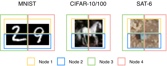
Refer to caption — (a) Observations at node 1/2 & demands at node 3/4.

Our evaluation compares the performance of our task-ware coding approach and other benchmark approaches (as in the last section) over a few standard ML datasets, including MNIST (LeCun et al. 1998), CIFAR-10, CIFAR-100 (Krizhevsky, Hinton et al. 2009) and SAT-6 (Basu et al. 2015). For MNIST, each data sample is a $28\times 28$ handwritten digit image, and we let $x$ be a horizontally-concatenated image ( $28\times 56$ ) of two images. Node 1 and 2 observe the upper and the lower half part of the concatenated image (both $14\times 56$ ) respectively. Task matrices $K^{(3)}$ and $K^{(4)}$ are formulated as follows: we pre-train a convolutional neural network (CNN) to classify original MNIST digits by their labels. Task matrix $K^{(3)}$ requires both the reconstruction of the feature map (i.e., the output of the first layer of CNN) of the left MNIST digit in the concatenated image, and the reconstruction of the concatenated image itself. Mathematically, we have

\displaystyle K^{(3)}=[\underbrace{\gamma\tilde{K}^{(3)\top}}_{\text{recon. of left feature map}},\underbrace{(1-\gamma)I}_{\text{recon. of conctenated image}}]^{\top},

(19)

where $\tilde{K}^{(3)}$ represents the mapping between $x$ and the feature map of the left MNIST digit, and $\gamma$ is a weight coefficient. Here we use $\gamma=0.9$ . Task matrix $K^{(4)}$ is formulated similarly while the feature map of the right MNIST digit is considered instead. For CIFAR-10/CIFAR-100/SAT-6, each data sample is a $32\times 32$ or $28\times 28$ colored image with 3 or 4 channels and we let $x$ represent the original image. We similarly let node 1 and 2 observe the upper and the lower half part of the image respectively, and let node 3 and node 4 require the reconstruction of the left and the right half part respectively. The setup is illustrated in Fig. 4(a). Other training details are provided in the appendix.

The evaluation result is shown in Fig. 4. In Fig. 4(b)-4(e), we plot the overall task loss $\mathcal{L}_{\text{total}}$ under different edge capacity $Z$ . In these figures, we see task-aware coding and coding benchmark approach outperform task-aware no coding and task-agnostic coding approach, and the overall task loss $\mathcal{L}_{\text{total}}$ of our task-aware coding approach is the closet to $\mathcal{L}_{\text{total, lb}}$ . The maximum improvements of overall task loss $\mathcal{L}_{\text{total}}$ for task-aware coding approach are 26.1%, 26.4%, 25.3% and 17.1% respectively, compared to task-agnostic coding approach; and are 9.1%, 103.3%, 97.8% and 28.4% respectively, compared to task-aware no coding approach. We also notice that, task-agnostic coding approach doesn’t always outperform task-aware no coding approach, and vice versa. Therefore, it is beneficial to combine network coding and task-awareness.

In Fig. 4(b), we compare the utilities of $\phi^{(5,6)},\phi^{(1,3)}$ and $\phi^{(2,4)}$ in terms of minimizing the overall task loss $\mathcal{L}_{\text{total}}$ when $Z=10$ , $\gamma=0.9$ . The three utilities are defined in a way such that their sums plus $\mathcal{L}_{\text{total}}$ is a fixed number (see appendix for the formal definition). We observe that the coding benchmark approach outperforms other approaches with respect to the utility of $\phi^{(5,6)}$ , but underperforms our task-aware coding approach by 4.2% with respect to the overall task loss $\mathcal{L}_{\text{total}}$ . This is because coding benchmark approach greedily determines the encoder parameters associated with edge $(5,6)$ first which however could not guarantee optimality. On the other hand, our task-aware coding approach tunes all the encoding and decoding parameters jointly and achieves a lower $\mathcal{L}_{\text{total}}$ .

Limitation. Our task-aware network coding problem defined in Eq. (9) is non-convex, and hence the adopted gradient descent method may converge to local optimum.

Conclusion

This paper considers task-aware network coding over butterfly network in real-coordinate space. We prove a lower bound $\mathcal{L}_{\text{total,lb}}$ of the total loss, as well as conditions for achieving $\mathcal{L}_{\text{total,lb}}$ . We also provide a machine learning algorithm in the general settings. Experimental results demonstrate that our task-aware coding approach outperforms the benchmark approaches under various settings.

Regarding future extension, although butterfly network is a representative topology in network coding, it is worthwhile to extend the analysis of the task-aware network coding problem to general networks. A similar $\mathcal{L}_{\text{total,lb}}$ can still be derived, yet the associated necessary condition and sufficient conditions for achieving $\mathcal{L}_{\text{total,lb}}$ depend on the specific network topology in a manner that needs further work to be fully understood.

References

Ahlswede et al. (2000) Ahlswede, R.; Cai, N.; Li, S.-Y.; and Yeung, R. W. 2000. Network information flow. IEEE Transactions on information theory, 46(4): 1204–1216.
Ahlswede and Korner (1975) Ahlswede, R.; and Korner, J. 1975. Source coding with side information and a converse for degraded broadcast channels. IEEE Transactions on Information Theory, 21(6): 629–637.
Avestimehr and Ho (2009) Avestimehr, A. S.; and Ho, T. 2009. Approximate capacity of the symmetric half-duplex Gaussian butterfly network. In 2009 IEEE Information Theory Workshop on Networking and Information Theory, 311–315. IEEE.
Basu et al. (2015) Basu, S.; Ganguly, S.; Mukhopadhyay, S.; DiBiano, R.; Karki, M.; and Nemani, R. 2015. Deepsat: a learning framework for satellite imagery. In Proceedings of the 23rd SIGSPATIAL international conference on advances in geographic information systems, 1–10.
Blau and Michaeli (2019) Blau, Y.; and Michaeli, T. 2019. Rethinking lossy compression: The rate-distortion-perception tradeoff. In International Conference on Machine Learning, 675–685. PMLR.
Chen et al. (2008) Chen, M.; Ponec, M.; Sengupta, S.; Li, J.; and Chou, P. A. 2008. Utility maximization in peer-to-peer systems. ACM SIGMETRICS Performance Evaluation Review, 36(1): 169–180.
Cheng et al. (2021) Cheng, J.; Pavone, M.; Katti, S.; Chinchali, S. P.; and Tang, A. 2021. Data Sharing and Compression for Cooperative Networked Control. In Thirty-Fifth Conference on Neural Information Processing Systems.
Doshi et al. (2010) Doshi, V.; Shah, D.; Médard, M.; and Effros, M. 2010. Functional compression through graph coloring. IEEE Transactions on Information Theory, 56(8): 3901–3917.
Dougherty, Freiling, and Zeger (2005) Dougherty, R.; Freiling, C.; and Zeger, K. 2005. Insufficiency of linear coding in network information flow. IEEE transactions on information theory, 51(8): 2745–2759.
Dubois et al. (2021) Dubois, Y.; Bloem-Reddy, B.; Ullrich, K.; and Maddison, C. J. 2021. Lossy Compression for Lossless Prediction. arXiv preprint arXiv:2106.10800.
Dunteman (1989) Dunteman, G. H. 1989. Principal components analysis. 69. Sage.
Feizi and Médard (2014) Feizi, S.; and Médard, M. 2014. On network functional compression. IEEE transactions on information theory, 60(9): 5387–5401.
Ho et al. (2006) Ho, T.; Médard, M.; Koetter, R.; Karger, D. R.; Effros, M.; Shi, J.; and Leong, B. 2006. A random linear network coding approach to multicast. IEEE Transactions on Information Theory, 52(10): 4413–4430.
Jaggi et al. (2005) Jaggi, S.; Sanders, P.; Chou, P. A.; Effros, M.; Egner, S.; Jain, K.; and Tolhuizen, L. M. 2005. Polynomial time algorithms for multicast network code construction. IEEE Transactions on Information Theory, 51(6): 1973–1982.
Koetter and Médard (2003) Koetter, R.; and Médard, M. 2003. An algebraic approach to network coding. IEEE/ACM transactions on networking, 11(5): 782–795.
Korner and Marton (1979) Korner, J.; and Marton, K. 1979. How to encode the modulo-two sum of binary sources (corresp.). IEEE Transactions on Information Theory, 25(2): 219–221.
Krizhevsky, Hinton et al. (2009) Krizhevsky, A.; Hinton, G.; et al. 2009. Learning multiple layers of features from tiny images.
LeCun et al. (1998) LeCun, Y.; Bottou, L.; Bengio, Y.; and Haffner, P. 1998. Gradient-based learning applied to document recognition. Proceedings of the IEEE, 86(11): 2278–2324.
Li, Yeung, and Cai (2003) Li, S.-Y.; Yeung, R. W.; and Cai, N. 2003. Linear network coding. IEEE transactions on information theory, 49(2): 371–381.
Liu et al. (2020) Liu, L.; Solomon, A.; Salamatian, S.; and Médard, M. 2020. Neural network coding. In ICC 2020-2020 IEEE International Conference on Communications (ICC), 1–6. IEEE.
Nakanoya et al. (2021) Nakanoya, M.; Chinchali, S.; Anemogiannis, A.; Datta, A.; Katti, S.; and Pavone, M. 2021. Co-design of communication and machine inference for cloud robotics. Robotics: Science and Systems XVII, Virtual Event.
Parag and Chamberland (2010) Parag, P.; and Chamberland, J.-F. 2010. Queueing analysis of a butterfly network for comparing network coding to classical routing. IEEE Transactions on Information Theory, 56(4): 1890–1908.
Shannon (1956) Shannon, C. 1956. The zero error capacity of a noisy channel. IRE Transactions on Information Theory, 2(3): 8–19.
Shannon et al. (1959) Shannon, C. E.; et al. 1959. Coding theorems for a discrete source with a fidelity criterion. IRE Nat. Conv. Rec, 4(142-163): 1.
Slepian and Wolf (1973) Slepian, D.; and Wolf, J. 1973. Noiseless coding of correlated information sources. IEEE Transactions on information Theory, 19(4): 471–480.
Soeda et al. (2011) Soeda, A.; Kinjo, Y.; Turner, P. S.; and Murao, M. 2011. Quantum computation over the butterfly network. Physical Review A, 84(1): 012333.
Vasisht, Shenoy, and Chandra (2021) Vasisht, D.; Shenoy, J.; and Chandra, R. 2021. L2D2: Low latency distributed downlink for LEO satellites. In Proceedings of the 2021 ACM SIGCOMM 2021 Conference, 151–164.
Whang et al. (2021) Whang, J.; Acharya, A.; Kim, H.; and Dimakis, A. G. 2021. Neural Distributed Source Coding. arXiv preprint arXiv:2106.02797.
Wu and Verdú (2010) Wu, Y.; and Verdú, S. 2010. Rényi information dimension: Fundamental limits of almost lossless analog compression. IEEE Transactions on Information Theory, 56(8): 3721–3748.
Wyner and Ziv (1976) Wyner, A.; and Ziv, J. 1976. The rate-distortion function for source coding with side information at the decoder. IEEE Transactions on information Theory, 22(1): 1–10.
Zhang et al. (2021) Zhang, G.; Qian, J.; Chen, J.; and Khisti, A. 2021. Universal Rate-Distortion-Perception Representations for Lossy Compression. arXiv preprint arXiv:2106.10311.

Appendix

Task-aware PCA Derivation

We define random variable $h=L^{-1}x\in\mathbb{R}^{n}$ and $\hat{h}=L^{-1}\hat{x}\in\mathbb{R}^{n}$ . Thus $\mathbb{E}_{h}[hh^{\top}]=\mathbb{E}_{x}[L^{-1}xx^{\top}L^{-\top}]=I$ . And we also define $D_{h}=L^{-1}D$ and $E_{h}=EL$ .

Then we have

$\displaystyle\mathcal{L}=$	$\displaystyle\mathbb{E}_{x}[\\|K(x-\hat{x})\\|_{2}^{2}]=\mathbb{E}_{h}[\\|KL(h-\hat{h})\\|_{2}^{2}]$
$\displaystyle=$	$\displaystyle\mathbb{E}_{h}[\\|KL(I-D_{h}E_{h})h\\|_{2}^{2}]$
$\displaystyle=$	$\displaystyle\mathbb{E}_{h}[\text{Tr}(KL(I-D_{h}E_{h})hh^{\top}(I-D_{h}E_{h})^{\top}L^{\top}K^{\top})]$
$\displaystyle=$	$\displaystyle\text{Tr}(KL(I-D_{h}E_{h})(I-D_{h}E_{h})^{\top}L^{\top}K^{\top})$	(20)

where $\text{Tr}(\cdot)$ denotes the trace of a matrix. We can verify that $D_{h}=E_{h}^{\top}(E_{h}E_{h}^{\top})^{-1}$ is a zero point of

\displaystyle\frac{\nabla\mathcal{L}}{\nabla D_{h}}=2L^{\top}K^{\top}KL(D_{h}E_{h}-I)E_{h}^{\top}.

(21)

So we plug $D_{h}=E_{h}(E_{h}E_{h}^{\top})^{-1}$ into Eq. 20 and get

\displaystyle\mathcal{L}=\text{Tr}(L^{\top}K^{\top}KL)-\text{Tr}(L^{\top}K^{\top}KLE_{h}^{\top}(E_{h}E_{h}^{\top})^{-1}E_{h}).

Therefore, we should find $E_{h}$ that maximizes $\text{Tr}(L^{\top}K^{\top}KLE_{h}^{\top}(E_{h}E_{h}^{\top})^{-1}E_{h})$ . Classical PCA dictates that $\text{Tr}(L^{\top}K^{\top}KLE_{h}^{\top}(E_{h}E_{h}^{\top})^{-1}E_{h})\leq\sum_{i=1}^{Z}\mu_{i}$ , i.e., $\mathcal{L}\geq\sum_{i=Z+1}^{n}\mu_{i}$ . And if the eigen-gap $\mu_{Z}-\mu_{Z+1}>0$ , the equality holds if and only if $\textup{\text{col}}(E_{h}^{\top})=\textup{\text{span}}(\{u_{1},u_{2},\cdots,u_{Z}\})$ , which is equivalent to $\textup{\text{col}}(E^{\top})=\textup{\text{span}}(\{L^{-\top}u_{1},L^{-\top}u_{2},\cdots,L^{-\top}u_{Z}\})$ .

Proof of Theorem 3 when $2Z>n$

Proof.

When $2Z>n$ , we have $r^{(3,4)}_{+}=r^{(3,4)}_{-}=n$ , and $r_{-}^{(1,3)}=a\geq n-Z$ , $r_{-}^{(2,4)}=b\geq n-Z$ . Therefore we aim to make $\textup{\text{col}}([\Phi^{(1,3)},\Phi^{(5,6)}])=\textup{\text{col}}([\Phi^{(2,4)},\Phi^{(5,6)}])=\mathbb{R}^{n}$ . Since butterfly network is symmetric, without loss of generality, we assume $a\leq b$ . And we denote the $i$ -th column vector of $L$ by $l_{i}$ .

We are able to find $\Phi^{(1,3)}$ , $\Phi^{(2,4)}$ and $\Phi^{(5,6)}$ such that $\mathcal{L}_{\text{total,lb}}$ is achievable, through the following three steps:

$\bullet$ i) Let the first $n-b$ column vectors of $\Phi^{(5,6)}$ be $l_{1}+l_{a+1},l_{2}+l_{a+2},\cdots,l_{n-b}+l_{a+n-b}$ , and the next $b-a$ column vectors of $\Phi^{(5,6)}$ be $l_{a+n-b+1},l_{a+n-b+2},\cdots,l_{n}$ ;

$\bullet$ ii) Let the first $n-b$ column vectors of $\Phi^{(1,3)}$ and $\Phi^{(2,4)}$ be $l_{1},l_{2},\cdots,l_{n-b}$ and $l_{a+1},l_{a+2},\cdots,l_{a+n-b}$ respectively;

$\bullet$ iii) Since $2Z>n$ , we have $Z-n+a+Z-n+b>a+b-n$ , i.e., the number of non-determined column vectors of $\Phi^{(5,6)}$ and $\Phi^{(1,3)}$ together is greater than the number of remaining vectors $l_{n-b+1},l_{n-b+2},\cdots,l_{a}$ . So we can assign $l_{n-b+1},l_{n-b+2},\cdots,l_{a}$ to the non-determined column vectors of $\Phi^{(5,6)}$ and $\Phi^{(1,3)}$ such that each vector among $l_{n-b+1},l_{n-b+2},\cdots,l_{a}$ is assigned at least once. In the end we assign the last $Z-n+b$ column vectors of $\Phi^{(1,3)}$ to the last $Z-n+b$ column vectors of $\Phi^{(2,4)}$ .

It can be verified that $\textup{\text{col}}([\Phi^{(1,3)},\Phi^{(5,6)}])=\textup{\text{col}}([\Phi^{(2,4)},\Phi^{(5,6)}])=\textup{\text{col}}(L)=\mathbb{R}^{n}$ . Therefore, $\mathcal{L}_{\text{total,lb}}$ is achievable. ∎

Further explanation of the task-aware coding benchmark approach

In the coding benchmark approach, our first step is to let the column vectors of $\Phi^{(5,6)}$ be the top- $Z$ normalized eigen-vectors of $S^{(3)}+S^{(4)}$ . This greedy step ensures $\mathcal{L}_{\text{total}}$ is minimized when node 3 and 4 receive $\phi^{(5,6)}$ only.

Next, to determine optimal $\Phi^{(1,3)}$ which further minimizes $\mathcal{L}_{\text{total}}$ as much as possible, we consider the following problem:

$\displaystyle\max_{\tilde{\Phi}^{(1,3)}\in\mathbb{R}^{n\times\min\{Z,c\}}}\quad$	$\displaystyle\tilde{\Phi}^{(1,3)\top}S^{(3)}\tilde{\Phi}^{(1,3)}$	(22)
s.t.	$\displaystyle\textup{\text{col}}(\tilde{\Phi}^{(1,3)})\subseteq V,$	(23)
	$\displaystyle\tilde{\Phi}^{(1,3)\top}\tilde{\Phi}^{(1,3)}=I,$	(24)

where $V=\{v\in\textup{\text{col}}([\Phi^{(5,6)},U^{(1)}])|v\perp w,\forall w\in\textup{\text{col}}(\Phi^{(5,6)})\}$ , and $c=\textup{\text{dim}}(\textup{\text{col}}([\Phi^{(5,6)},U^{(1)}]))-Z$ is the dimension of $V$ . The following $\tilde{\Phi}^{(1,3)}$ is an optimal solution for the considered problem: we formulate a matrix $W\in\mathbb{R}^{n\times c}$ whose column vectors form an orthogonal basis of $V$ , and then let the column vectors of $\tilde{\Phi}^{(1,3)}$ be $W$ times the top- $\min\{Z,c\}$ normalized eigen-vectors of $W^{\top}S^{(3)}W$ . For fixed $\Phi^{(5,6)}$ , we know the optimal $\Phi^{(1,3)}$ that minimizes $\mathcal{L}_{\text{total}}$ should satisfy $\textup{\text{col}}([\Phi^{(1,3)},\Phi^{(5,6)}])=\textup{\text{col}}([\tilde{\Phi}^{(1,3)},\Phi^{(5,6)}])$ . Yet in general $\tilde{\Phi}^{(1,3)}\nsubseteq U^{(1)}$ , so we cannot assign the column vectors of $\tilde{\Phi}^{(1,3)}$ to the column vectors of $\Phi^{(1,3)}$ directly. Therefore, we let the first $\min\{Z,c\}$ column vectors of $\Phi^{(1,3)}$ be the vectors in $\textup{\text{col}}(U^{(1)})$ that extend a basis of $\textup{\text{col}}(\Phi^{(5,6)})$ to a basis of $\textup{\text{col}}([\tilde{\Phi}^{(1,3)},\Phi^{(5,6)}])$ . Other non-determined column vectors of $\Phi^{(1,3)}$ , if any, can be arbitrary vectors in $\textup{\text{col}}(U^{(1)})$ .

We also use the similar idea to determine the column vectors of $\Phi^{(2,4)}$ .

Training Details

Table 1: Training Details

Application	Num of Samples (Train/Test)	Num of Epochs	Batch Size	Learning Rate	Runtime
Simulation	64/64	2000	64	$0.05$	$<24$ hrs
MNIST	30000/5000	20	64	$5\times 10^{-3}$	$<24$ hrs
CIFAR-10	50000/10000	20	64	$5\times 10^{-3}$	$<24$ hrs
CIFAR-100	50000/10000	20	64	$5\times 10^{-3}$	$<24$ hrs
SAT-6	324000/81000	5	64	$5\times 10^{-3}$	$<72$ hrs

Both our simulation and our evaluation run on a personal laptop with 2.7 GHz Intel Core I5 processor and 8-GB 1867 MHz DDR3 memory. Our code is based on Pytorch and the Adam optimizer is used. The number of samples (train/test), number of epochs, batch size, learning rate and corresponding runtime (for the whole experiment) are summarized in Table 1. Note that our simulation is based on synthetic data, so we only need a training/testing dataset that satisfies $\mathbb{E}_{x}[x]=\bm{0},\Psi=I$ and hence $2n=64$ samples are enough. The publicly-available MNIST, CIFAR-10, CIFAR-100 and SAT-6 datasets do not have a stated license online.

Moreover, our evaluation for MNIST also requires a pre-trained CNN classifier for $28\times 28$ images, which is composed of two consecutive convolution layers and a final linear layer. The number of input channels, the number of output channels, kernel size, stride and padding for two convolution layers are 1, 16, 5, 1, 2 and 16, 32, 5, 1, 2 respectively, and ReLU activation and max pooling with kernel size 2 are used after each convolution layer. The final linear layer has input size 1568 and output size 1.

We also provide our code in the supplementary material and will make it publicly-available after the review process.

Overall Task Losses of Task-agnostic Coding Approach for Simulation

Figure 5: Simulation result with synthetic data of task-agnostic coding approach: overall task loss

\mathcal{L}_{\text{total}}

under different

r_{+}^{(3,4)}

(left) and different

a

(right).

Fig. 5 shows the overall task losses of task-agnostic coding approach for the two simulations. For the purpose of comparison we also plot the overall task losses of our task-aware coding approach (same values as in Fig. 3). It clearly illustrates that task-agnostic coding approach performs more poorly than the task-aware coding approach.

Definitions of the Utilities in Evaluation

We first define the utility of $\phi^{(5,6)}$ . We can find normalized vectors $\xi_{1},\cdots,\xi_{d}$ that form an orthogonal basis of $\textup{\text{col}}(\Phi^{(5,6)})$ , where $d=\textup{\text{dim}}(\textup{\text{col}}(\Phi^{(5,6)}))$ . Then the utility of $\phi^{(5,6)}$ is defined as $\sum_{j=1}^{d}\xi_{j}^{\top}(S^{(3)}+S^{(4)})\xi_{j}$ , which is essentially the minimum achievable overall task loss difference between the case when node 3 and 4 receive nothing and when they receive $\phi^{(5,6)}$ only. For task-aware coding benchmark approach, according to Further explanation of the task-aware coding benchmark approach, the utility of $\phi^{(5,6)}$ equals the sum of the top- $Z$ eigen-values of $S^{(3)}+S^{(4)}$ .

We next define the utility of $\phi^{(1,3)}$ . We can find normalized vectors $\chi_{1},\cdots,\chi_{e}$ that extend $\xi_{1},\cdots,\xi_{d}$ to an orthogonal basis of $\textup{\text{col}}([\Phi^{(1,3)},\Phi^{(5,6)}])$ , where $e=\textup{\text{dim}}(\textup{\text{col}}([\Phi^{(1,3)},\Phi^{(5,6)}]))-d$ . Then the utility of $\phi^{(1,3)}$ is defined as $\sum_{j=1}^{e}\chi_{j}^{\top}S^{(3)}\chi_{j}$ , which is essentially the minimum achievable overall task loss difference between the case when node 3 receives $\phi^{(5,6)}$ only and when it receives both $\phi^{(1,3)}$ and $\phi^{(5,6)}$ .

The utility of $\phi^{(2,4)}$ is defined similarly as $\phi^{(1,3)}$ .

Comparison of the Reconstructed Images in Evaluation

In Fig. 6, we compare a few reconstructed images for different approaches in our evaluation (when $Z=10,\gamma=0.9$ ). For task-aware approaches, since the task loss of node 3 is dominated by the reconstruction of the left feature map respectively, we see the left part of the reconstructed image at node 3 has a higher quality compared to the right part. And for node 4 we have similar observations. On the other hand, for task-agnostic coding approach, the quality difference between the left part and the right part is not as obvious as the task-aware approaches.

Task-Aware Network Coding Over Butterfly Network

Abstract

Introduction

Preliminaries

Network Coding with a Classical Example

Task-aware PCA

Problem Formulation

Analysis

Lower bound ℒtotal,lb\mathcal{L}_{\text{total,lb}}

Theorem 1.

Proof.

Necessary condition

Theorem 2.

Proof.

Sufficient Conditions

Theorem 3.

Proof.

Corollary 4.

Proof.

Corollary 5.

Proof.

Algorithm

Evaluation

Conclusion

References

Appendix

Task-aware PCA Derivation

Proof of Theorem 3 when 2​Z>n2Z>n

Proof.

Further explanation of the task-aware coding benchmark approach

Training Details

Overall Task Losses of Task-agnostic Coding Approach for Simulation

Definitions of the Utilities in Evaluation

Comparison of the Reconstructed Images in Evaluation

Lower bound $\mathcal{L}_{\text{total,lb}}$

Proof of Theorem 3 when $2Z>n$